Distributionally balanced sampling designs via minimum tactical configurations

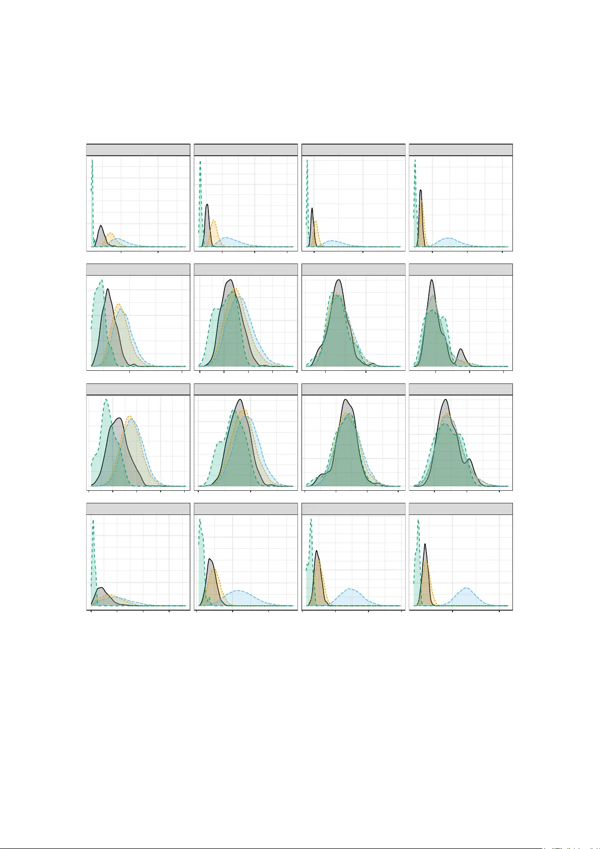
Distributionally balanced sampling designs via minim um tactical configurations An ton Grafström ∗ and Wilmer Pren tius † Departmen t of F orest Resource Managemen t, Sw edish Univ ersity of Agricultural Sciences, Umeå, Sweden Marc h 26, 2026 Abstract Distributionally balanced sampling designs are lo w-discrepancy probabilit y designs obtained b y minimizing the expected discrepancy b et ween the auxiliary -v ariable distribution of a random sample and the target p opulation distribution. Existing constructions rely on circular population sequences, which restrict the design space b y forcing samples to b e con tiguous blo cks of a sequence. W e prop ose a new con- struction based on minimum tactical configurations that remov es this top ological constrain t. The resulting designs are fixed-size, ha ve equal inclusion probabilities, and b elong to the class with minimum feasible configuration size. W e dev elop b oth a simple initialization v alid for arbitrary p opulation and sample sizes and a spatial initialization that yields a lo wer initial exp ected discrepancy , together with a sim- ulated annealing algorithm for optimization within this class. In simulations and empirical examples, the proposed metho d outp erforms state-of-the-art alternatives in terms of distributional fit, balance, and spatial spread. Keyw ords: Balanced sampling, Energy distance, Spatial sampling, Probabilit y sampling, V ariance reduction. ∗ Email: anton.grafstrom@slu.se, h ttps://orcid.org/0000-0002-4345-4024 † Email: wilmer.prentius@slu.se, h ttps://orcid.org/0000-0002-3561-290X 1 1 In tro duction Distributionally Balanced Designs (DBD) w ere in tro duced to construct probability sam- ples whose auxiliary distribution appro ximates the p opulation distribution in a strong metric sense (Grafström & Pren tius, 2026). The k ey idea is to define a probability mea- sure on a space of samples such that, when a sample is drawn according to the design, its empirical auxiliary v ariable distribution closely matches that of the population. This ob- jectiv e is formalized by minimizing the exp ected energy distance (Székely & Rizzo, 2013) b et ween the random sample and the p opulation. Existing DBD implemen tations rely on arranging the population in to a circular se- quence and selecting samples as con tiguous blo cks with random start. While this con- struction guaran tees equal inclusion probabilities, it in tro duces a strong topological con- strain t: eac h unit must form a distributionally represen tative sample with its immediate neigh b ors in the sequence. As a result, the admissible design space is restricted to samples that resp ect this ordering. In this pap er, we remov e this constrain t by shifting from sequence-based designs to tactical configurations (binary 1-designs) of minimum size, see e.g. Beth et al. (1999, Ch. 1). Instead of ov erlapping wi ndo ws of a p ermutation, w e construct a finite list of samples suc h that: 1. eac h sample has size n , 2. eac h unit app ears in the same minim um feasible n um b er of samples, 3. the exp ected energy distance b etw een the auxiliary v ariable distribution of a uni- formly drawn sample and the population is (approximately) minimized. Systematic sampling is w ell known to ac hiev e the minim um p ossible supp ort size for fixed-size equal-probability designs, but it represents an extreme solution that only enforces inclusion probabilities (Pea et al., 2007). Its defining structure relies on a de- terministic ordering of the p opulation, and the resulting samples inherit distributional prop erties that critically dep end on how this ordering aligns with the auxiliary v ariables. Still, ordered systematic sampling can be viewed as an intuitiv e w a y to achiev e appro xi- mate distributional balance in the univ ariate case. If the p opulation is ordered by the size of an auxiliary v ariable, then each sample’s empirical distribution will tend to b e close to the p opulation distribution. In contrast, the prop osed DBD-TC framework op erates on a large class of designs. Within this class, it explicitly selects designs whose samples approximately minimize the exp ected distributional discrepancy with resp ect to a set of auxiliary v ariables. Relativ e to circular DBD (Grafström & Prentius, 2026), the present work contributes (i) a practical solution to selecting approximately distributionally balanced samples from a larger class of designs, and (ii) tw o different initialization algorithms v alid for arbitrary ( N , n ) . The remainder of the pap er is organized as follows. Section 2 introduces the method- ological framework, defines tactical configuration designs, establishes the minimum size of a tactical configuration, and presents initializations that pro duce a v alid tactical configu- ration for arbitrary p opulation and sample sizes. Section 3 outlines a sto chastic optimiza- tion algorithm to refine the design with incremental up dates that achiev e connectivity of the admissible design space. Section 4 provides examples that illustrate the difference in p erformance b etw een DBD-TC and some alternativ e designs. Section 5 concludes with a summary and directions for future research. 2 2 Metho dological framew ork This section establishes the theoretical foundations. W e first define the structure of the tactical configurations and deriv e the theoretical b ound for their size. Then, w e introduce the energy distance as the design criterion and describ e metho ds for generating v alid initial configurations for arbitrary p opulation and sample sizes. 2.1 P opulation and design structure Let U = { 1 , 2 , . . . , N } denote a finite p opulation of size N , where each unit i ∈ U is asso ciated with a vector of auxiliary v ariables x i ∈ R p . W e seek a probability sampling design with a fixed sample size n and equal first-order inclusion probabilities π i = n/ N for all i ∈ U . W e first define the combinatorial structure from which samples are dra wn. Definition 1 (T actical configuration) . A design matrix D = [ d 1 | d 2 | · · · | d M ] of samples d k ∈ { 0 , 1 } N is a tactical configuration if: 1. P N i =1 d ik = n > 0 for al l k = 1 , . . . , M ; 2. P M k =1 d ik = c > 0 for al l i ∈ U , i.e. al l samples have fixe d size n , and al l units app e ar in exactly c samples. Based on this structure, w e define the corresp onding sampling design. Definition 2 (T actical configuration sampling design) . A sampling design is a tactical configuration design if it is c onstructe d by sele cting a c olumn of D uniformly at r andom. Be c ause D may c ontain duplic ate samples, the pr ob ability of sele cting a unique sample d is given by p ( d ) = P ( δ = d ) = m ( d ) M , wher e δ is the r andom sample and m ( d ) is the multiplicity of d in D . By definition, in a tactical configuration design, the first- and second-order inclusion probabilities are exactly π i = P M k =1 d ik M , π ij = P M k =1 d ik d j k M . Throughout the pap er, the column v ectors d k of a tactical configuration D are referred to as samples, and d ij refers to elements of D , while d i refer to the i -th elemen t of a sp ecific sample vector d . 2.2 Minim um tactical configurations In general, a tactical configuration ma y contain duplicate samples (when c > 1 ). This im- plies that the size of the design’s supp ort (the set of unique samples S with strictly p ositive probabilit y) is b ounded b y the size of the configuration, i.e., |S | ≤ M . F or computational and practical efficiency , w e aim to k eep the configuration as small as possible. 3 Definition 3 (Minim um tactical configuration) . A tactic al c onfigur ation D is minimum if its size M , and thus the multiplicity c onstant c , ar e minimize d. A design b ase d on this structur e is c al le d a minim um tactical configuration design , and M , c ar e c al le d minimum tactical configuration parameters . The minim um p ossible size is determined by the greatest common divisor of N and n . Prop osition 1 (Theoretical b ound on configuration size) . L et g = gcd( N , n ) . The size of a tactic al c onfigur ation must b e at le ast M = N/g , with e ach unit app e aring exactly c = n/g times. Pr o of. In the N × M configuration D , eac h column sums to n , and eac h ro w sums to c . Hence M n = N c , which rearranges to M /c = N/n . T o minimize M and c sub ject to the constraint that b oth must b e p ositive in tegers, we divide N and n by their greatest common divisor g . This yields the absolute minim um in teger v alues c = n/g and M = N /g . Circular DBD has support size N via a sequence-based construction, whereas Prop osi- tion 1 shows that a minimum tactical configuration has size N /g . Therefore, the supp ort size of DBD-TC is at most N /g , whic h is strictly smaller than N when g > 1 , without imp osing ordering constrain ts. 2.3 Energy distance F ollowing Grafström & Pren tius (2026), distrib utional balance is quantified using the energy distance. Let F d and F U b e the empirical distributions of { x i : d i = 1 } and { x i : i ∈ U } , resp ectively . Also, let X , X ′ b e indep enden t random vectors distributed according to F d , and let Z , Z ′ b e indep endent random vectors distributed according to F U . The energy distance betw een these distributions is defined as E ( F d , F U ) = 2 E ∥ X − Z ∥ − E ∥ X − X ′ ∥ − E ∥ Z − Z ′ ∥ , (1) where ∥ · ∥ denotes the Euclidean distance. Let Φ i = 1 N X k ∈ U ∥ x i − x k ∥ , i ∈ U. F or a sample d , the computable energy distance derived from (1) b ecomes E ( F d , F U ) = X i ∈ U Φ i  2 d i n − 1 N  − X i ∈ U X j ∈ U d i n d j n ∥ x i − x j ∥ . (2) 2.4 Design ob jectiv e Let P denote the set of all tactical configurations D that satisfy the minim um size condi- tions deriv ed in Prop osition 1. The DBD-TC ob jective is to find a tactical configuration D ∗ b y minimizing the exp ected energy distance across the configuration: D ∗ ∈ arg min D ∈P E [ E ( F δ , F U )] , 4 where E [ E ( F δ , F U )] = ¯ E ( D ) = 1 M M X k =1 E ( F d k , F U ) . Th us, the target of optimization is the configuration itself. Due to the large size of P , w e use sim ulated annealing to find a configuration D ◦ that pro duces an exp ected energy distance close to that of D ∗ . As in circular DBD (Grafström & Prentius, 2026), the use of the energy distance is motiv ated b y its connection to reduced Horvitz–Thompson v ariance when the empirical auxiliary distribution of a randomly selected sample is close to that of the p opulation. 2.5 A simple constructiv e initialization T o p erform the optimization, we first require a v alid starting p oin t D ∈ P . Constructing a tactical configuration where every sample has size n and every unit app ears exactly c times corresp onds to a combinatorial design problem. While the space of suc h designs is large, a v alid instance can be generated efficiently b y mapping a p ermutation of the p opulation on to the indices of the sample sets using mo dular arithmetic. The follo wing randomized cyclic assignment metho d guarantees a v alid initial configuration for any pair N , n . Lemma 1. L et v ∈ { 0 , 1 } M b e a ve ctor such that exactly c entries ar e 1. Then a minimum tactic al c onfigur ation D is the matrix whose r ows ar e the first N cyclic shifts of v ⊺ . Pr o of. Assume D ∈ { 0 , 1 } N × M to ha v e the size of a minimum tactical configuration, i.e. M = N/g and c = n/g . By the definition of v , the rows of D sum to c . A full cycle of v is completed after M ro ws, and after g rotations are completed, the columns of D sum to cg = n . Example 1 (Constructive initialization) . F or a p opulation of size N = 6 , a sample of size n = 4 has minimum tactic al c onfigur ation p ar ameters M = 3 , c = 2 , as g = 2 . An arbitr ary cyclic ve ctor is v = [1 , 1 , 0] ⊺ , which yields the minimum tactic al c onfigur ation matrix D =         1 1 0 0 1 1 1 0 1 1 1 0 0 1 1 1 0 1         . If D is a minim um tactical configuration, and P is a (random) p ermutation matrix of size N × N , then P D is also a minim um tactical configuration. 2.6 Sampling-based initialization While the simple initialization ensures a v alid tactical configuration, the resulting con- figuration t ypically exhibits a high initial distributional discrepancy . Here, w e pro- p ose a sampling-based initialization. The pro cess, which constructs the configuration D ∈ { 0 , 1 } N × M b y sequen tially filling each sample, is defined in Algorithm 1. 5 Algorithm 1 Sampling-based initialization of tactical configuration 1: Input: Population and sample size N , n . Fixed size sample generator f : [0 , 1] N → { 0 , 1 } N . 2: Compute: Minim um tactical configuration parameters M , c ; initial budget b 0 = 1 c . 3: for k = 1 to M do 4: Calculate the remaining budget for the units: 5: b k ← b k − 1 − d k − 1 , where d 0 = 0 . 6: Set inclusion probabilities: 7: p k ← b k / ( M − k + 1) . 8: Select a sample using f : 9: d k ← f ( p k ) . 10: end for 11: return T actical configuration D = [ d 1 | d 2 | · · · | d M ] . The pro cess in Algorithm 1 is guaran teed for any fixed-size sample generator f that pro vides the prescrib ed inclusion probabilities p k , as b k ∈ { 0 , . . . , M − k + 1 } N ensures v alid inclusion probabilities, and P i ∈ U b ik = n ( M − k + 1) implies that p k sums to n . Using the lo cal piv otal metho d (Grafström et al., 2012) as the sample generator f guaran tees a well-spread sample of exactly n units at eac h step. This approach yields an initial configuration in whic h each sample is generated b y a spatially balanced pro cedure. F or the sim ulated annealing pro cess, this "warm start" may reduce the total num b er of iterations required to lo cate a near-optimal design. 3 Algorithm Algorithm 2 presen ts the pseudo-co de for finding an optimized configuration D ◦ , starting from an initial state D (0) . The optimization op erates ov er P using elementary transitions defined b y pairwise exc hanges. Sp ecifically , tw o samples (columns) d k , d l with k  = l are selected and a swap b etw een units i and j , where d ik = 1 and d j l = 1 , is admissible if d il = 0 and d j k = 0 . See Figure 1 for an illustration. At each iteration, tw o random units are selected from t w o samples. If a sw ap is admissible, the units are mov ed according to the simulated annealing procedure (see e.g. Kirkpatric k et al., 1983). Figure 1: Illustration of an admissible swap b etw een a unit i in d k ( d ik = 1 ) and a unit j in d l ( d j l = 1 ). The sw ap is admissible as d il = 0 and d j k = 0 (before the swap). 6 Algorithm 2 Optimization through sim ulated annealing 1: Input: 2: Initial state of the configuration D (0) . 3: Iterations R , initial temp T (0) , and co oling rate α . 4: Compute: Exp ected energy distance ¯ E (0) = ¯ E ( D (0) ) . 5: Initialize: Best state pair D ◦ ← D (0) ; and ¯ E ◦ ← ¯ E (0) . 6: for r = 1 to R do 7: D ( r ) ← D ( r − 1) , ¯ E ( r ) ← ¯ E ( r − 1) . 8: Select tw o samples k , l with k  = l ; 9: Select units i, j uniformly from the set of units in samples k , l resp ectively , 10: i.e. suc h that d ( r ) ik = d ( r ) j l = 1 . 11: if d ( r ) il = d ( r ) j k = 0 then 12: Sw ap the units 13: d ( r ) ik ← 0; d ( r ) il ← 1 ; 14: d ( r ) j l ← 0; d ( r ) j k ← 1 ; 15: and compute the exp ected energy distance ¯ E ( r ) . 16: if ¯ E ( r ) < ¯ E ◦ then 17: New b est state D ◦ ← D ( r ) , ¯ E ◦ ← ¯ E ( r ) . 18: else if ¯ E ( r ) ≥ ¯ E ( r − 1) and U (0 , 1) ≥ exp( − ( ¯ E ( r ) − ¯ E ( r − 1) ) /T ( r − 1) ) then 19: Reject swap and reset D ( r ) ← D ( r − 1) , ¯ E ( r ) ← ¯ E ( r − 1) . 20: end if 21: end if 22: Up date temp erature T ( r ) ← α T ( r − 1) . 23: end for 24: return Optimized configuration D ◦ . As a tactical configuration is an N × M binary incidence matrix with constant sums of rows and columns, and an admissible sw ap is exactly a 2 × 2 in terc hange, the margins are preserv ed during admissible swaps. Ryser (1957) established that the class of such matrices is connected under elementary in terchanges, whic h corresp onds to the pairwise sw aps defined in our algorithm. This connectivit y prop ert y ensures that lo cal sto chastic optimization metho ds, such as simulated annealing, can explore the entire admissible design space. In Append ix A, we show that the cost of calculating the exp ected energy distance in eac h step is limited b y O ( n ) and pro vide a remark on parallel up dates. In App endix B, w e pro vide some strategies that can b e helpful in dealing with large p opulations. A random sample δ is obtained by drawing a sample uniformly at random from the optimized configuration D ◦ . An efficient implemen tation of Algorithm 2 is a v ailable in the rsamplr R pack age (Pren tius, 2025). 4 Sim ulation Here, w e compare the DBD-TC against some existing designs based on four differen t qualit y measures: the mean energy distance, the mean spatial balance (Stev ens & Olsen, 2004), the mean lo cal balance (Pren tius & Grafström, 2024) and the mean balance de- viation. Balance deviation (BD) is measured for all auxiliary v ariables b y the Euclidean 7 distance b etw een the HT-estimators and the true totals B D ( δ ) = ∥ ˆ X δ − X ∥ , where ˆ X δ = X i ∈ U x i π i δ i , X = X i ∈ U x i . F or all measures, low er v alues are better. As a baseline, w e include simple random sam- pling. Comp etitors are the lo cal piv otal metho d (LPM), the lo cal cub e metho d (LCub e) and circular DBD. W e use the same set of examples as Grafström & Prentius (2026) to illustrate the difference b etw een circular DBD and DBD-TC. Example 2 (Deca y of the exp ected energy distance) . W e gener ate d a synthetic p opu- lation of size N = 1000 with p = 5 auxiliary variables. The auxiliary variables x i = ( x i 1 , . . . , x ip ) ⊤ wer e dr awn indep endently fr om a uniform distribution on [0 , 1] . The sam- ple size was chosen as n = 50 . Figur e 2 il lustr ates the de c ay of the exp e cte d ener gy distanc e in an optimization run and c omp ar es with a cir cular DBD run. 0.004 0.005 0.006 0M 2M 4M 6M 8M 10M Figure 2: Exp ected energy distance of Circular DBD (solid gray) and DBD-TC (dashed green) at iterations up to 10M, ± 2 standard deviations, for a fixed-sized sample of n = 50 and p = 5 auxiliary v ariables (i.e. M = 20 samples). As can b e seen from Figure 2, DBD-TC reaches a mean energy distance that seems unattainable with circular DBD. Example 3 (Comparisons with some existing designs) . T o evaluate the p erformanc e of the pr op ose d metho d acr oss varying de gr e es of c omplexity, we gener ate d synthetic p opulations of size N = 1000 with p auxiliary variables, wher e p ∈ { 2 , 5 , 10 , 20 } . The auxiliary variables x i = ( x i 1 , . . . , x ip ) ⊤ wer e dr awn indep endently fr om a uniform distribution on [0 , 1] . W e sele cte d samples of fixe d size n = 50 with e qual inclusion pr ob abilities (for p = 5 we also sele cte d samples of sizes n = 100 and n = 200 ). F or the c omp etitor metho ds (SRS, LPM, LCub e), we p erforme d 10,000 indep endent Monte Carlo r ep etitions using the rsamplr R p ackage. F or cir cular DBD, we evaluate d 8 the p erformanc e on al l N p ossible samples define d by the optimize d se quenc e (i.e., for the c omplete design) after 10 7 iter ations. DBD-TC was also optimize d using 10 7 iter ations. T able 1 summarizes the r esults for dimensions p = 2 , 5 , 10 , 20 and sample size n = 50 . The r esulting distributions of the differ ent metrics under DBD-TC, cir cular DBD, LCub e and LPM ar e shown in Figur e 3. T able 2 shows the r esult for p = 5 auxiliary variables when incr e asing the sample size to n = 100 and n = 200 . T able 1: Simulation results for N = 1000 , n = 50 across dimensions p ∈ { 2 , 5 , 10 , 20 } . The table compares the metho ds on distributional fit using mean energy distance (mean E ), spatial balance (mean SB), lo cal balance (mean LB), and balance deviation of auxiliary v ariables (mean BD). Lo wer v alues indicate b etter performance. Dims Metho d E SB LB BD 2 SRS 0.0099 0.3375 0.1459 49.79 LPM 0.0015 0.0879 0.0769 10.50 LCUBE 0.0013 0.0825 0.0751 7.97 Circular DBD 0.0010 0.0612 0.0646 4.88 DBD-TC 0.0007 0.0430 0.0559 1.02 5 SRS 0.0167 0.2518 0.1831 84.38 LPM 0.0069 0.1342 0.1464 36.50 LCUBE 0.0053 0.1265 0.1429 15.07 Circular DBD 0.0046 0.1157 0.1391 12.44 DBD-TC 0.0040 0.1028 0.1327 4.23 10 SRS 0.0241 0.3493 0.2739 122.96 LPM 0.0145 0.2768 0.2566 74.54 LCUBE 0.0104 0.2702 0.2551 25.79 Circular DBD 0.0096 0.2629 0.2529 23.41 DBD-TC 0.0086 0.2587 0.2509 11.84 20 SRS 0.0343 0.5651 0.4329 175.59 LPM 0.0252 0.5151 0.4242 129.13 LCUBE 0.0171 0.5179 0.4239 45.15 Circular DBD 0.0167 0.5158 0.4233 41.76 DBD-TC 0.0151 0.4846 0.4201 25.33 F rom Example 3, we conclude that the DBD-TC pro vides the b est distributional fit across all dimensions. F rom T able 2 we note that as the sample size grows, the effect of the improv ed distributional fit remains. Example 4 (Ev aluation using the Meuse dataset) . W e evaluate DBD-TC using the Meuse dataset (Peb esma, 2004), which c onsists of 164 lo c ations in a river flo o d plain. After r emoval of two lo c ations with missing values, we use d the r emaining N = 162 lo c ations as our p opulation. W e c omp ar e SRS, the lo c al pivotal metho d (LPM), the lo c al cub e metho d (LCub e) and cir cular DBD against the pr op ose d DBD-TC for a sample size of n = 20 . A l l designs, exc ept SRS, use five standar dize d auxiliary variables: c o or dinates ( x, y ), elevation (elev), or ganic matter (or g), and c opp er c onc entr ation (Cu). In LCub e, al l five auxiliary variables ar e use d for b oth spr e ad and b alanc e. Distanc es wer e c alculate d 9 T able 2: Sim ulation results for N = 1000 with p = 5 auxiliary v ariables at increased sam- pling fractions ( n = 100 and n = 200 ). The table compares the metho ds on distributional fit using mean energy distance (mean E ), spatial balance (mean SB), lo cal balance (mean LB), and balance deviation of auxiliary v ariables (mean BD). Low er v alues indicate b etter p erformance. Size Metho d E SB LB BD 100 SRS 0.0078 0.2560 0.1295 57.72 LPM 0.0028 0.1400 0.1021 21.33 LCUBE 0.0021 0.1412 0.1017 7.65 Circular DBD 0.0019 0.1331 0.0999 6.37 DBD-TC 0.0016 0.1210 0.0959 1.98 200 SRS 0.0035 0.2781 0.0942 38.70 LPM 0.0011 0.1590 0.0740 12.37 LCUBE 0.0008 0.1729 0.0761 3.89 Circular DBD 0.0007 0.1630 0.0742 3.12 DBD-TC 0.0006 0.1569 0.0731 1.00 using standar dize d auxiliary variables. The tar get variables ar e the c onc entr ation of zinc (Zn), le ad (Pb), and c admium (C d). The cir cular DBD and DBD-TC wer e optimize d over 10 7 iter ations. T able 3: Mean energy distance, RRMSE of HT-estimators, and 95% CI co verage for the Meuse dataset ( N = 162 , n = 20 ). F or LPM, LCub e, circular DBD and DBD-TC w e applied the lo cal mean v ariance estimator with k = 2 neighbors. A total of 10 7 iterations w as used. Metho d Zn Pb Cd Cu elev org E SB LB RRMSE SRS 0.168 0.154 0.234 0.124 0.055 0.099 0.126 0.363 0.408 LPM 0.102 0.094 0.120 0.053 0.016 0.043 0.044 0.270 0.176 LCub e 0.099 0.087 0.120 0.043 0.018 0.033 0.038 0.277 0.188 Circular DBD 0.088 0.077 0.118 0.028 0.014 0.021 0.032 0.265 0.165 DBD-TC 0.084 0.071 0.083 0.011 0.004 0.007 0.026 0.253 0.150 Co verage SRS 0.915 0.914 0.907 0.918 0.847 0.927 LPM 0.945 0.960 0.928 0.960 0.990 0.973 LCub e 0.961 0.972 0.942 0.990 0.943 0.995 Circular DBD 0.994 0.988 0.895 1.000 0.969 1.000 DBD-TC 1.000 1.000 1.000 1.000 1.000 1.000 The results for Example 4, summarized in T able 3, demonstrate that DBD-TC achiev es the lo west mean energy distance, indicating sup erior distributional matc hing. F or the Meuse example, this discrepancy reduction pro vides substan tial efficiency gains. In par- ticular, DBD-TC outp erforms the state-of-the-art methods. Finally , the cov erage results sho w that DBD-TC provides conserv ativ e statistical inference. Only SRS w as consistently b elo w the nominal co verage rate. 10 BD , 2 BD , 5 BD , 10 BD , 20 LB, 2 LB, 5 LB, 10 LB, 20 SB, 2 SB, 5 SB, 10 SB, 20 Energy , 2 Energy , 5 Energy , 10 Energy , 20 0 10 20 30 0 30 60 0 50 100 150 100 200 0.04 0.06 0.08 0.10 0.12 0.10 0.15 0.20 0.24 0.28 0.32 0.40 0.45 0.50 0.1 0.2 0.05 0.10 0.15 0.20 0.25 0.2 0.4 0.5 1.0 1.5 0.0015 0.0025 0.006 0.009 0.012 0.01 0.02 0.02 0.03 0.04 Figure 3: Distributions of the differen t metrics under three designs with sample size n = 50 . Colors represen t the designs: green is DBD-TC, gra y is circular DBD ( 10 7 iterations), orange is LCub e, blue is LPM. First row: energy distance. Second ro w: the lo cal balance measure. Third ro w: spatial balance. F ourth ro w: balance deviation. Columns: n um b er of auxiliary v ariables. 11 5 Final remarks This pap er has extended the distributionally balanced sampling framework by relaxing the top ological constraints of circular designs. By framing the problem as a search for optimal tactical configurations, w e established that distributionally balanced samples can b e constructed without relying on the linear ordering of the population. This c haracteri- zation ac hieves the theoretical low er b ound on the configuration size, M = N / gcd( N , n ) , whic h nev er exceeds the p opulation s ize. Computationally , the shift from ov erlapping windows to indep endent sets offers dis- tinct adv an tages. The prop osed sim ulated annealing algorithm p erforms up dates in O ( n ) time and op ens up the p ossibilit y of parallel up dates on large problems. This mak es DBD-TC particularly attractive for large-scale applications where the computational cost of minimizing the energy distance would otherwise be prohibitiv e. As for circular DBD, w e suggest using an approximate v ariance estimator based on lo cal means (see e.g., Grafström & Pren tius, 2026). The fast implementation in the R pack age rsamplr (Prentius, 2025) makes it easy for practitioners to use DBD-TC in applications. It can b e used to produce designs that excel in distributional balance. F or more than 20 y ears, the cub e method has b een the gold standard for balanced sampling by fo cusing on the realization of samples that satisfy linear constraints. Ho wev er, our results demonstrate that realization-based metho ds are fundamentally limited. The lo cal pivotal metho d is also realization-based and builds a single sample through sequen tial random decisions that cannot be c h anged. By shifting to design construction through supp ort optimization, all samples are jointly optimized. This means that errors can b e more ev enly distributed across the supp ort. An y design-level ob jective can b e optimized o ver the support, whereas realization-based metho ds are limited to constructive rules for individual samples. In that sense, realization-based methods are inheren tly more restrictiv e. Thus, for an y given design-lev el ob jective, supp ort optimization can attain an optim um at least as go o d as that ac hiev able within an y realization-based sub class. This explains wh y the prop osed distributionally balanced designs achiev e sup erior balance and spatial spread in our examples compared to realization-based metho ds. F uture researc h includes extension to unequal inclusion probabilities and, if p ossi- ble, dev elopment of a less conserv ative v ariance estimator for distributionally balanced sampling. References Beth, T., Jungnic kel, D., & Lenz, H. (1999). Design Theory: V olume 1. Cam bridge Uni- v ersity Press. Deville, J.-C. & Tillé, Y. (2004). Efficien t balanced sampling: The cub e metho d. Biometrika , 91(4), 893-912. Grafström, A., Lundström, N. L., & Sc helin, L. (2012). Spatially balanced sampling through the piv otal metho d. Biometrics , 68(2), 514-520. Grafström, A., & Prentius, W. (2026). Distributionally balanced sampling designs. arXiv. h ttps://doi.org/10.48550/arXiv.2603.11916 12 Kirkpatric k, S., Gelatt Jr, C. D., & V ecchi, M. P . (1983). Optimization b y simulated annealing. Scienc e , 220(4598), 671-680. P ea, J., Qualité, L., & Tillé, Y. (2007). Systematic sampling is a minimum supp ort design. Computational statistics & data analysis , 51(12), 5591-5602. P eb esma, E. J. (2004). Multiv ariable geostatistics in S: the gstat pack age. Computers & Ge oscienc es , 30(7), 683-691. Pren tius, W., & Grafström, A. (2024). Ho w to find the b est sampling design: A new measure of spatial balance. Envir onmetrics , 35(7), e2878. Pren tius, W. (2025). rsamplr: Sampling Algorithms and Spatially Balanced Sampling. R pac k age v ersion 0.2.0. https://cran.r-pro ject.org/web/pac k ages/rsamplr/. Ryser, H. J. (1957). Combinatorial prop erties of matrices of zeros and ones. Canadian Journal of Mathematics , 9, 371-377. Stev ens Jr, D. L., & Olsen, A. R. (2004). Spatially balanced sampling of natural resources. Journal of the Americ an Statistic al Asso ciation , 99(465), 262-278. Szék ely , G. J., & Rizzo, M. L. (2013). Energy statistics: A class of statistics based on distances. Journal of Statistic al Planning and Infer enc e , 143(8), 1249-1272. A Efficien t up date of the ob jectiv e function A.1 Incremen tal up dates Consider a curren t tactical configuration D and an admissible sw ap b etw een units u, v in samples d a , d b , where d ua = d v b = 1 , creating the new configuration D ′ . F rom (2) we get the total energy of the configuration as E ( D ) = M X k =1 E ( F d k , F U ) =  2 c n − M N  X i ∈ U Φ i − M X k =1 X i ∈ U X j ∈ U d ik n d j k n ∥ x i − x j ∥ . The change in total energy is ∆ E = E ( D ′ ) − E ( D ) = 1 n 2 X i ∈ U X j ∈ U  d ia d j a − d ′ ia d ′ j a + d ib d j b − d ′ ib d ′ j b  ∥ x i − x j ∥ . As d ia d j a − d ′ ia d ′ j a = 0 for an y pair i, j not including u, v , and vice v ersa for b , w e get ∆ E = 2 n 2 X i ∈ U (( d ia − d ′ ib ) ∥ x i − x u ∥ + ( d ib − d ′ ia ) ∥ x i − x v ∥ ) = = 2 n 2 X i ∈ U \{ u,v } ( d ia − d ib ) ( ∥ x i − x u ∥ − ∥ x i − x v ∥ ) , using the fact that d ia d ua − d ′ ia d ′ ua = d ia and d ia d v a − d ′ ia d ′ v a = − d ′ ia , and analogously for sample b . The final equality follows as for i / ∈ { u, v } , w e ha v e d ia = d ′ ia and d ib = d ′ ib . As 13 only units in exactly one of the samples d a or d b affect the change in energy , the total computational cost to ev aluate ∆ E is O ( n ) . A.2 P arallel up dates Since the design ob jective is defined as a sum of sample energies, any sw aps inv olving disjoin t pairs of samples are non-in teracting in the ob jectiv e. Consequen tly , up to ⌊ M / 2 ⌋ up dates can be p erformed in parallel within a single iteration, p oten tially pro viding sub- stan tial computational sp eedups for desi gns with large supp ort sizes. B Sampling of large p opulations B.1 Stratification F or extremely large p opulations, the DBD-TC framework can b e applied within strata de- fined by auxiliary v ariables, as in the Blo ck-DBD approach (Grafström & Prentius, 2026). Eac h stratum is treated indep endently , allowing lo cal minim um-size configurations, O ( n ) incremen tal up dates, and parallel swaps. The stratified samples can then b e com bined to form a global design that maintains distributional represen tativeness, making the metho d suitable for v ery large-scale applications. B.2 LPM-based compression for large p opulations When the p opulation size N is v ery large, the minim um configuration size M = N / gcd( N , n ) implied b y Prop osition 1 may still b e computationally prohibitive. In suc h cases, the DBD-TC construction can b e preceded b y a randomized p opulation compression step that reduces the effective configuration size in a controlled manner. Sp ecifically , one ma y c ho ose a p ositiv e in teger M ∗ that is smaller than or equal to ⌊ N /n ⌋ , and define a reduced p opulation size N ∗ = M ∗ n . Then a subset U ∗ ⊂ U with | U ∗ | = N ∗ is selected using the lo cal piv otal metho d (LPM) with equal inclusion probabilities. The empirical distribution F U ∗ pro vides an appro ximation of the p opulation distribution F U , and the approximation error b ecomes small when N ∗ ≫ n . Conditionally on U ∗ , the DBD-TC construction is applied with p opulation size N ∗ and sample size n . This pro cedure pro vides correct un- conditional inclusion probabilities and introduces a tunable accuracy–complexit y tradeoff that remov es arithmetic discontin uities and makes optimization feasible for very large p opulations. Ho w ever, it only pro duces a conditional design. Example 5 (LPM-based compression for large p opulations) . Consider a p opulation of size N = 10 6 and a sample size n = 51 . In this c ase, gcd( N , n ) = 1 , which implies a minimum c onfigur ation size of M = 10 6 . T o r e duc e the c onfigur ation while pr eserving exact inclusion pr ob abilities, we cho ose a smal ler tar get size, e.g., M ∗ = ⌊ N /n ⌋ = 19 , 607 . This c orr esp onds to a r e duc e d p opulation size of N ∗ = M ∗ n = 999 , 957 . By sele cting the N ∗ units for U ∗ fr om U via the lo c al pivotal metho d, we ar e effe c- tively r ounding the weights W i = M ∗ ( n/ N ) to inte ger fr e quencies n i ∈ { 0 , 1 } such that P n i = N ∗ . The DBD-TC is then c onstructe d by p artitioning these 999 , 957 units into 19 , 607 samples. Unc onditional ly, e ach unit i ∈ U is include d in a r andom sample S with pr ob ability: Pr( i ∈ S ) = Pr( i ∈ U ∗ ) Pr( i ∈ S | i ∈ U ∗ ) = M ∗ n N 1 M ∗ = n N = 51 10 6 . 14 This pr o duc es an exc el lent appr oximation to the distributional ly b alanc e d design that would have b e en obtaine d on the ful l p opulation, while avoiding the arithmetic disc ontinuity of the gcd function and dr amatic al ly r e ducing the c omputational bur den. 15