Continuous-Time Learning of Probability Distributions: A Case Study in a Digital Trial of Young Children with Type 1 Diabetes
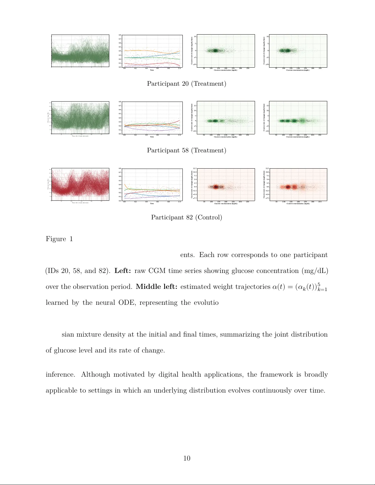
Understanding how biomarker distributions evolve over time is a central challenge in digital health and chronic disease monitoring. In diabetes, changes in the distribution of glucose measurements can reveal patterns of disease progression and treatm…
Authors: Antonio Álvarez-López, Marcos Matabuena
Con tin uous-Time Learning of Probabilit y Distributions: A Case Study in a Digital T rial of Y oung Children with T yp e 1 Diab etes An tonio Álv arez-López ∗ Univ ersidad A utónoma de Madrid and Marcos Matabuena † Mohamed bin Za yed Univ ersit y of Articial In telligence Marc h 26, 2026 Abstract Understanding ho w biomark er distributions ev olve o v er time is a cen tral c hallenge in digital health and chronic disease monitoring. In diab etes, changes in the distribu- tion of glucose measuremen ts can rev eal patterns of disease progression and treatment resp onse that con v en tional summary measures miss. Motiv ated by a 26-week clini- cal trial comparing the closed-lo op insulin delivery system t:slim X2 with standard therap y in children with t yp e 1 diabetes, w e prop ose a probabilistic framework to mo del the con tin uous-time evolution of time-indexed distributions using con tin uous glucose monitoring data (CGM) collected every v e min utes. W e represent the glu- cose distribution as a Gaussian mixture, with time-v arying mixture weigh ts gov erned b y a neural ODE. W e estimate the mo del parameter using a distribution-matc hing criterion based on the maximum mean discrepancy . The resulting framework is in- terpretable, computationally ecien t, and sensitiv e to subtle temporal distributional c hanges. Applied to CGM trial data, the metho d detects treatment-related improv e- men ts in glucose dynamics that are dicult to capture with traditional analytical approac hes. K eywor ds: Con tinuous glucose monitoring; Digital health; Distribution dynamics; Neural ODEs; Gaussian mixture mo dels; Maxim um Mean Discrepancy . ∗ Univ ersidad A utónoma de Madrid † Mohamed bin Za yed Univ ersity of Articial Intelligence 1 1 In tro duction Characterizing the distribution of a random v ariable is a classical problem in statistics Silv erman ( 2018 ) and remains a central c hallenge in mo dern mac hine learning LeCun et al. ( 2015 ), where accurate distribution represen tations are essen tial for tasks such as text generation and automated rep orting Meskó & T opol ( 2023 ). More broadly , many scientic questions require understanding not only individual observ ations but also ho w the full distribution of a pro cess ev olv es o v er time. This p ersp ective is particularly relev ant in clinical applications. In digital health, estimating the distribution of individual physiological time-series data o v er sp ecic time p erio ds enables the construction of individual represen tations that cap- ture their underlying physiological pro cesses with high precision Matabuena et al. ( 2021 ), Matabuena & P etersen ( 2023 ), Ghosal et al. ( 2023 ). Recent studies show that, when used prop erly , such representations can rev eal clinically relev an t patterns that traditional (non- digital) biomarkers do not detect Katta et al. ( 2024 ), Matabuena, Ghosal, Aguilar, Keshet, W agner, F ernández Merino, Sánc hez Castro, Zipunniko v, Onnela & Gude ( 2025 ), Park et al. ( 2025 ), Matabuena et al. ( 2026 ). In this pap er, motiv ated by digital health applications, w e study the problem of con tin- uously estimating a time-indexed distribution from sequentially observ ed data. The goal is to learn ho w the underlying distribution ev olves and to represen t that ev olution in a w ay that is b oth exible and interpretable. Standard approac hes are often unsatisfac- tory in this setting. Extending classical k ernel densit y estimators (KDEs) Chacón & Duong ( 2018 ) to include time t ypically leads to a strong sensitivit y to tuning parameters and to the curse of dimensionality , while ow-based generative mo dels Papamakarios et al. ( 2021 ) ma y b e less interpretable and can require substantial training eorts. Semiparametric al- ternativ es oer partial remedies. F or example, time-v arying mo dels suc h as Generalized 2 A dditiv e Mo dels for Lo cation, Scale, and Shape (GAMLSS) Rigb y & Stasinop oulos ( 2005 ) alleviate some of these issues, but most implemen tations are designed for scalar responses and ma y impose rigid functional forms. More recen t m ultilevel functional approaches based on functional-quan tile representations Matabuena & Crainicean u ( 2026 ) oer interpretabil- it y but rely on linear dynamics, whic h limits their abilit y to capture complex non-linear relationships and m ultiv ariate distributions. T o address these limitations, w e prop ose a con tin uous-time Gaussian mixture framew ork in whic h distributional dynamics are represen ted through time-v arying mixture weigh ts go v erned by a neural ODE. Problem form ulation Let . F or eac h , let denote a random vector representing the quan tit y of in terest at time . Its (cum ulative) distribution function is d (1) where inequalit y and integral are tak en comp onen t-wise when , and is the probabilit y density function (when it exists) at time . Our target ob ject is , or equiv alen tly , the density curve , from whic h can b e reco v ered through ( 1 ). In practice, ho w ev er, the pro cess is not observ ed contin uously in time. Instead, data are av ailable on a discrete time grid (2) A t each , we observe a sample dra wn from the distribution , (3) Dep ending on the application, these observ ations may be treated either as approximately indep enden t snapshots across time or as part of a longitudinal setting with temp oral de- 3 p endence. In b oth cases, the statistical problem is to recov er a coheren t con tinuous-time represen tation of the underlying distributional dynamics from these discrete observ ations. W e mo del eac h as a Gaussian mixture with comp onents, where and are the mean v ector and co v ariance matrix of the th Gaussian comp onen t, respectively , and the w eigh t vector lies in the probability simplex (4) The comp onent means and co v ariance matrices are shared o ver time, while the mixture w eigh ts v ary contin uously with . This shared-dictionary representation is natural in our motiv ating application, where the Gaussian comp onents may b e viewed as latent glycemic regimes whose locations and scales remain relativ ely stable o v er the study perio d, while their relativ e prev alence c hanges o ver time. A t the same time, this is a strong structural assumption: b y allowing temp oral v ariation only through the mixture weigh ts, we trade some mo deling exibility for in terpretability and a more parsimonious characterization of distributional change. W e mo del the resulting w eigh t dynamics through a neural ODE. As increases, Gaussian mixtures pro vide substantial appro ximation exibility , whereas for mo derate v alues of the resulting weigh t tra jectories remain smo oth, in terpretable and statistically tractable. Digital health motiv ation and distributional data analysis Our motiv ation comes from the analysis of glucose distributions in longitudinal diab etes trials Battelino et al. ( 2023 ), where glucose is constan tly recorded using con tinuous glu- cose monitoring (CGM). Under free-living conditions, individual glucose time series can- 4 not b e directly aligned, making the ra w temp oral sto chastic pro cess dicult to compare b et w een participants Ghosal & Matabuena ( 2024 ), Matabuena et al. ( 2021 ), Matabuena, Ghosal, Aguilar, Keshet, W agner, F ernández Merino, Sánc hez Castro, Zipunniko v, On- nela & Gude ( 2025 ). In this setting, the time-v arying probability distribution pro vides a more natural biomark er to characterize the evolution of glucose metabolism Katta et al. ( 2024 ), P ark et al. ( 2025 ), Matabuena et al. ( 2021 ). Compared to conv entional CGM summary statistics—such as mean glucose or time-in-range metrics—this represen tation con v eys richer information by capturing the full sp ectrum of low, mo derate and high glu- cose v alues within a unied functional prole Matabuena et al. ( 2021 ), Katta et al. ( 2024 ). More broadly , distributional data analysis Ghosal et al. ( 2023 ), Szabó et al. ( 2016 ) is an emerging area that treats probability distributions, or collections of them, as statistical ob- jects for unsup ervised and supervised learning, including the prediction of clinical outcomes Matabuena et al. ( 2021 ). Biomedical applications are among their most prominent use cases. In digital health, measurements collected by con tin uous glucose monitors, accelerometers, or imaging mo dalities suc h as functional magnetic resonance imaging (fMRI) are increas- ingly represen ted through empirical distributions that serve as laten t descriptions of under- lying ph ysiological processes Ghosal et al. ( 2025 ), Ghosal & Matabuena ( 2024 ), Matabuena, Ghosal, Aguilar, Keshet, W agner, F ernández Merino, Sánchez Castro, Zipunnik o v, Onnela & Gude ( 2025 ), Matabuena et al. ( 2022 ). In recent y ears, sev eral regression frameworks ha v e b een prop osed in whic h predictors, resp onses, or b oth are represen ted as probabil- it y distribution functions Matabuena & Petersen ( 2023 ), Ghosal et al. ( 2025 ), Ghosal & Matabuena ( 2024 ), Ghosal et al. ( 2026 ), Matabuena, Ghosal, Meiring & Petersen ( 2025 ). A related line of work represen ts probability distributions as random objects in metric spaces and dev elops statistical pro cedures for that setting (see, e.g., Lugosi & Matabuena ( 2024 )). Despite this progress, there remains no general framework for mo deling mo derate- 5 to high-dimensional distributions that sim ultaneously oers exibilit y and in terpretabilit y . The metho dology introduced here is in tended to help bridge this gap. Con tributions This paper develops a statistical framew ork to mo del the contin uous-time ev olution of probabilit y distributions from longitudinal data and shows its practical v alue in a case study of digital health. Our main contributions are as follo ws: 1. W e prop ose a general framew ork for mo deling the dynamics of multiv ariate probabil- it y distributions in con tin uous time b y com bining Gaussian mixture represen tations with neural ODE smo othing, yielding an in terpretable estimator. 2. W e introduce an estimation pro cedure based on a Maxim um Mean Discrepancy ob- jectiv e Gretton et al. ( 2012 ). This av oids the need to sp ecify and optimize a full lik eliho o d under temporal dep endence, while pro ducing a simple dierentiable loss with closed-form expressions for Gaussian mixtures under Gaussian kernels. A t eac h time p oin t, the empirical loss function takes the form of a V-statistic Sering ( 2009 ). 3. W e demonstrate the practical utilit y of the prop osed methods in a biomedical appli- cation by analyzing contin uous glucose monitoring data from a longitudinal trial in y oung c hildren with t yp e 1 diab etes W adw a et al. ( 2023 ). Our approac h pro vides clin- ically meaningful insights on glucose dynamics and the benets of the new closed-lo op insulin system compared to standard therap y , including treatment-related c hanges that are less apparent from con ven tional analytical approaches. 4. W e pro vide theoretical supp ort for the rst stage of the pro cedure, prior to tempo- ral smo othing. In particular, w e establish an approximation result for the shared- dictionary represen tation and a nite-sample b ound for the minimum-MMD estima- tor of the mixture weigh ts at each observ ed time p oint. The mathematical results 6 and the corresp onding proofs are given in the Supplementary Material (Section A ). 2 Case study: closed-lo op insulin deliv ery in y oung c hildren with t yp e 1 diab etes T reatment of t yp e 1 diabetes in young c hildren remains a particularly c hallenging task Sc ho elw er et al. ( 2024 ), W are et al. ( 2024 ). In children y ounger than 6 y ears of age, insulin doses are small, while fo o d intak e, meal timing, and physical activit y are often unpredictable, making dosing decisions esp ecially dicult. Y oung c hildren ma y also exhibit greater glycemic v ariability than older c hildren and adults. As a result, treatmen t strategies and therap eutic goals are often harder to dene in this population, and only a limited n um b er of hybrid closed-lo op systems Kitagaw a et al. ( 2025 ), Hughes et al. ( 2023 ) hav e receiv ed formal approv al from the U.S. F o o d and Drug Administration for c hildren under 6 years of age. This case study is motiv ated b y a randomized clinical trial ev aluating the t:slim X2 insulin pump with Control-IQ T echnology (T andem Diab etes Care) in y oung children with type 1 diab etes W adwa et al. ( 2023 ). The t:slim X2 system is a h ybrid closed-loop device that uses con tin uous glucose monitoring (CGM) measurements to guide automated insulin delivery through basal rate adjustmen ts and correction b oluses every ve minutes. Although this tec hnology has b een extensiv ely studied in older children, adolescen ts and adults Bec k et al. ( 2023 ), Stahl-Pehe et al. ( 2025 ), the evidence in children under 6 years of age has remained relativ ely limited. The trial W adw a et al. ( 2023 ) enrolled 102 children aged 2–5 years and randomized them in a 2:1 ratio to closed-lo op con trol ( ) or standard care ( ) for 26 weeks. Our goal in revisiting these data is not simply to reassess treatmen t ecacy using conv entional 7 endp oin ts, but to examine whether a distributional represen tation of CGM measuremen ts can rev eal treatmen t-related c hanges in glucose regulation that are less apparen t from standard summary measures. This question is motiv ated b y the gro wing need for analytical to ols that c haracterize glucose b eha vior beyond conv entional CGM summaries, suc h as mean glucose, time in range, and related comp ositional metrics. Although these summaries are clinically useful, they do not fully capture the ric hness of CGM data, which con tain information on m ultiple time scales, including short-term uctuations and rate of c hange. These features ma y reect clinically signican t dierences in glucose regulation and resp onse to treatment. Recen t w ork has prop osed gluc o density as a functional representation of a glucose time series through the marginal distribution of CGM measurements Matabuena et al. ( 2021 ). This framew ork can capture asp ects of glucose b eha vior that are not fully summarized b y stan- dard scalar metrics. Ho w ev er, a univ ariate glucodensity does not directly capture temp oral dynamics, such as whether glucose lev els c hange rapidly or more gradually ov er time. T o address this limitation, m ultiv ariate extensions incorp orate dynamic features Matabuena, Ghosal, Aguilar, Keshet, W agner, F ernández Merino, Sánchez Castro, Zipunnik o v, Onnela & Gude ( 2025 ), including the rate of change and, p otentially , acceleration, through join t densit y representations such as or . These multiv ariate representations pro vide a natural framework for studying how glucose lev els and glucose dynamics evolv e o v er time. In this paper, w e reanalyze the trial data W adwa et al. ( 2023 ) using a m ultiv ariate glu- co densit y framew ork Matabuena, Ghosal, Aguilar, Keshet, W agner, F ernández Merino, Sánc hez Castro, Zipunniko v, Onnela & Gude ( 2025 ) designed to capture b oth the distribu- tion of glucose v alues and key asp ects of glucose dynamics. W e summarize each participan t’s time-v arying distribution using a Gaussian mixture mo del with comp onents and 8 a shared component dictionary ov er time. The w eigh ts of the participant-specic mixture then dene longitudinal trajectories that characterize the ev olution of individual glucose distributions and, in the multiv ariate setting, the corresp onding glucose dynamics during follo w-up. Figure 1 illustrates the structure of the data and the proposed representation for three represen tativ e participants (tw o in the in terv en tion group and one in the con trol group). F or each participan t, w e sho w the ra w CGM time series, the estimated tra jectories of the mixture w eights, and the tted biv ariate densities based on glucose and its rate of c hange at the b eginning and end of the trial. Our primary objective in this case study is to assess whether this distributional frame- w ork yields clinically in terpretable comparisons b etw een treatment groups and whether incorp orating glucose dynamics into the gluco densit y represen tation provides additional insigh t b eyond conv entional summary measures. In the original article, W adwa et al. ( 2023 ) found that glucose lev els were within the target range for a greater prop ortion of time under the closed-lo op system than in standard care. How ev er, the authors did not nd clear dierences in the time sp ent in other glycemic ranges such as h yp oglycemia or, for some subgroups of individuals, in other common diabetes biomarkers such as glycated hemoglobin (HbA1c). W e analyze this dataset from a distributional persp ectiv e with the goal of enric hing and extending the original analysis. 3 Metho dology W e introduce a Gaussian mixture framew ork for learning time-v arying distributions from longitudinal data observed on a discrete time grid. The metho d represen ts distributional dynamics in contin uous time, yields interpretable sub ject-sp ecic trajectories, and supp orts distributional comparisons across groups (interv en tion arms) and downstream statistical 9 0 50 100 150 200 250 Time slot (5-min intervals) 0 50 100 150 200 250 300 350 400 Glucose (mg/dL) 0.0 0.2 0.4 0.6 0.8 1.0 T ime 0.0 0.1 0.2 0.3 0.4 0.5 0.6 0.7 0.8 50 100 150 200 250 300 350 Glucose concentration (mg/dL) 10 5 0 5 10 Glucose rate of change (mg/dL/time) 50 100 150 200 250 300 350 Glucose concentration (mg/dL) 10 5 0 5 10 Glucose rate of change (mg/dL/time) P articipan t 20 (T reatment) 0 50 100 150 200 250 Time slot (5-min intervals) 0 50 100 150 200 250 300 350 400 Glucose (mg/dL) 0.0 0.2 0.4 0.6 0.8 1.0 T ime 0.0 0.1 0.2 0.3 0.4 0.5 0.6 0.7 0.8 50 100 150 200 250 300 350 Glucose concentration (mg/dL) 10 5 0 5 10 15 Glucose rate of change (mg/dL/time) 50 100 150 200 250 300 350 Glucose concentration (mg/dL) 10 5 0 5 10 15 Glucose rate of change (mg/dL/time) P articipan t 58 (T reatment) 0 50 100 150 200 250 Time slot (5-min intervals) 0 50 100 150 200 250 300 350 400 Glucose (mg/dL) 0.0 0.2 0.4 0.6 0.8 1.0 T ime 0.0 0.1 0.2 0.3 0.4 0.5 0.6 0.7 0.8 50 100 150 200 250 300 350 Glucose concentration (mg/dL) 7.5 5.0 2.5 0.0 2.5 5.0 7.5 10.0 12.5 Glucose rate of change (mg/dL/time) 50 100 150 200 250 300 350 Glucose concentration (mg/dL) 7.5 5.0 2.5 0.0 2.5 5.0 7.5 10.0 12.5 Glucose rate of change (mg/dL/time) P articipan t 82 (Control) Figure 1: Individual participan t analysis for the biv ariate mo del (glucose and its rst deriv ativ e) using Gaussian comp onents. Each row corresp onds to one participant (IDs 20, 58, and 82). Left: raw CGM time series sho wing glucose concentration (mg/dL) o v er the observ ation p erio d. Middle left: estimated weigh t tra jectories learned b y the neural ODE, represen ting the ev olution of the mixture prop ortions ov er normalized time . Middle right and right: con tours of the tted biv ariate Gaussian mixture density at the initial and nal times, summarizing the joint distribution of glucose lev el and its rate of c hange. inference. Although motiv ated b y digital health applications, the framew ork is broadly applicable to settings in whic h an underlying distribution evolv es con tinuously o v er time. 10 3.1 Bac kground Our prop osed framew ork com bines t w o mathematical ingredien ts: maxim um mean discrep- ancy , which we use to t the mo del at the observed time p oints, and neural ODEs, whic h mo del the contin uous-time ev olution of the underlying distribution. Maxim um Mean Discrepancy . T o compare probability distributions and on a common measurable space , we use the maximum me an discr ep ancy (MMD) Gretton et al. ( 2012 ), Muandet et al. ( 2017 ). T o do so, MMD represents each distribution as an element in a Hilb ert space. Let b e the repro ducing kernel Hilbert space (RKHS) induced by a positive denite k ernel . If is a probabilit y distribution suc h that d (e.g., if is bounded), then the kernel me an emb e dding of , denoted by , is w ell dened: d F ormally , MMD ev aluates the distance b etw een t w o distributions as the -norm of the dierence b et w een their em b eddings: MMD (5) where i.i.d. and i.i.d. . If the mapping is injectiv e, equiv alen tly if the k ernel is char acteristic , then MMD denes a v alid metric, satisfying MMD if and only if , see Srip erum budur et al. ( 2011 ), Sejdinovic et al. ( 2013 ). Throughout the pap er, w e x and use the Gaussian k ernel: exp (6) 11 where is a bandwidth parameter. Since the Gaussian k ernel is b ounded and c har- acteristic, the kernel mean embedding is well-dened, and the associated MMD denes a metric on probabilit y distributions. In practice, the c hoice of strongly impacts the sensitivit y of the metric to dierent scales. W e set it using the median heuristic Garreau et al. ( 2017 ): is c hosen as the median of the pairwise Euclidean distances betw een sample p oin ts. In tuition. MMD measures ho w far apart tw o distributions are in the feature space induced b y the kernel . In our setting, at each observ ed time p oint in the grid ( 2 ), w e use MMD to compare the empirical distribution associated with the observ ations in ( 3 ) to a tted Gaussian mixture distribution. Wh y MMD? (i) With a Gaussian k ernel, the discrepancy b etw een an empirical distribu- tion and a Gaussian mixture admits closed-form terms, whic h leads to stable and computa- tionally ecient updates. (ii) Characteristic k ernels yield well-posed tting ob jectiv es. (iii) Empirical evidence suggests that MMD-based pro cedures are more robust than lik eliho o d- based metho ds under temp oral dep endence and mo del missp ecication Chérief-Ab dellatif & Alquier ( 2022 ), Alquier & Gerb er ( 2024 ), Gao et al. ( 2021 ), Alquier et al. ( 2023 ). Neural ODEs. W e replace discrete la y ers by the con tinuous evolution of a hidden state where is a learnable v ector eld, typically parameterized b y a m ultila y er p erceptron. The tra jectory is computed n umerically , and gradients with resp ect to can b e obtained using adjoin t metho ds Massaroli et al. ( 2020 ). Neural ODEs ha v e b een used to mo del laten t tra jectories in contin uous time Kidger et al. ( 2020 ), R ubanov a et al. ( 2019 ), Jia & Benson ( 2019 ), including in biomedical applications 12 Qian et al. ( 2021 ). In our framework, the laten t tra jectory is used to parameterize the mixture weigh ts o v er time. This provides a smooth con tin uous-time interpolation of the w eigh ts estimated on the discrete grid ( 2 ), without imposing a rigid parametric form on their evolution. Wh y a neural ODE? Our ob ject of in terest is the con tin uous-time distribution of CGM in free-living environmen ts, where measuremen ts are irregular and not directly aligned across participan ts. Mo deling the weigh t tra jectories through a neural ODE is adv antageous for sev eral reasons. (i) It naturally accommodates irregularly sampled data without re- quiring ad ho c grid alignmen t, while its con tinuous nature mitigates sensor noise. (ii) It pro vides a parameter-ecien t framew ork (a single vector eld enco des arbitrary depth) to generate smo oth, con tin uous laten t trajectories. (iii) By con trast, discrete sequence mo dels W ang ( 2024 ), W u et al. ( 2023 ) are eectiv e in forecasting ra w traces but do not directly target the con tin uous-time distributional dynamics central to our aims. 3.2 Our mo del W e mo del the contin uous-time densit y as a Gaussian mixture: (7) where the comp onent means and co v ariance matrices are shared across time, while the mixing weigh ts v ary contin uously with (within the simplex). This shared-dictionary structure mak es the represen tation comparable across b oth time p oin ts and individuals. This mo deling choice is theoretically grounded in Wiener–T aub erian approximation argu- men ts Wiener ( 1932 ). As detailed in Theorem A.1 , under mild regularity conditions, these shared-dictionary mixtures can uniformly appro ximate any contin uous curv e of densities 13 in . Specically , for any , choosing a suciently large ensures: sup In practice, we x a mo derate to preserve in terpretabilit y , selecting its v alue based on the sp ecic application (cf. Section 5 ). F ormally , our mo del is dened b y the time-dep endent parameter v ector: whose eective dimension at any xed is . 3.2.1 Discrete-time MMD tting Giv en the observ ation grid and the sample —recall ( 2 ) and ( 3 )—, we dene the empirical distribution by A t each discrete time step , we t a static Gaussian mixture b y minimizing MMD , where is the distribution with densit y . W e use a Gaussian kernel of the form ( 6 ), with bandwidth selected by the median heuristic from the sample . By expanding the squared MMD, the ob jectiv e function reduces to a con v enien t quadratic form in the mixing w eigh ts : MMD (8) where dep ends solely on the empirical data and can therefore b e omitted from the minimization, while the matrix and the 14 v ector admit closed-form expressions for their en tries: det Id exp Id det Id exp Id Optimization. W e minimize ( 8 ) using the following alternating sc heme: 1. Initialization. W e run -means clustering Jain ( 2010 ) on to initialize the parameters: the means are the cen troids of the iden tied clusters; are the empirical co v ariance matrices of the p oin ts within eac h cluster; and the initial weigh ts corresp ond to the proportion of data p oints at time assigned to cluster . 2. Lo cal up date. F or each , k eeping means and co v ariances xed, we up date the w eigh ts via the quadratic program: argmin (9) where is a vector of ridge hyperparameters that impro v es numerical conditioning and stabilizes the solution when Gaussian comp onents b ecome nearly collinear in the RKHS feature space. 3. Global up date. Up date and iterativ ely via (Adam) gradien t descent on the MMD ob jectiv e, keeping the curren t w eigh ts xed. 3.2.2 Con tin uous-time weigh t evolution Once the discrete-time weigh ts are tted, we use a con tin uous-time mo del for their ev olution. On , we solve: (10) 15 where is a multila y er p erceptron (architecture and solv er hyperpa- rameters are rep orted in T able 2 ), and then map to v alid mixture w eigh ts b y a simplex normalization op erator. Dene 1 (11) (with the con ven tion that if 1 , w e replace b y 1 for a small ). The parameters are optimized b y matching the ODE predictions to the tted weigh ts : (12) where is obtained b y integrating ( 10 ) and applying ( 11 ) at time , and is a ridge hyperparameter. P erm utation symmetry . Because are shared o v er time and k ept xed after the global t, comp onent lab els are anchored. The neural ODE stage only ev olves , so tra jectories cannot exc hange lab els, removing p ermutation ambiguit y . Remark 3.1. As an alternative to the simplex normalization based on the p ositiv e part (see ( 11 )), one may evolv e logits and set softmax If has strictly p ositive comp onen ts, then c ho osing log 1 arbitrary ensures , since softmax is in v ariant under shifts b y 1 . If some components of are zero, one may initialize with 1 for a small and set log . 16 4 Sim ulation study W e b enc hmark nite-sample p erformance against represen tativ e baselines. Unlik e comp et- ing approac hes, our metho d prioritizes in terpretability through the time-v arying w eigh ts for . The results indicate that this emphasis on interpretabilit y does not come at the exp ense of accuracy: the prop osed metho d remains comp etitiv e in statistical error and, in sev eral multiv ariate settings, outp erforms the alternatives. A dditional details are provided in the Supplementary Material (Section C ). 5 Case Study: CGM T rial F rom a distributional data analysis p ersp ective, the ob jectiv e of this case study is to sho w that the prop osed metho dology can lev erage the thousands of glucose measurements recorded by contin uous glucose monitoring (CGM) more eectively than con ven tional scalar summaries. Standard CGM metrics are naturally em b edded in the glucodensity framew ork Matabuena et al. ( 2021 ); ho w ev er, our ob jective here is to sho w that m ultiv ariate functional represen tations can also reveal clinically signican t asp ects of glucose regulation that are not fully captured by standard summaries alone. F rom a mo deling p ersp ective, our goal is to illustrate the interpretabilit y of the prop osed framew ork to c haracterize longitudinal dierences in glycemic proles betw een the t wo study arms. In particular, w e fo cus on iden tifying distributional dierences b etw een treat- men t and control ov er time and on assessing whether incorp orating glucose dynamics through rates of change improv es the c haracterization of these dierences b etw een groups o v er the course of follo w-up. 17 Preliminaries and scien tic questions As describ ed in Section 2 , our analysis is motiv ated by data from the randomized clinical trial published in the New England Journal of Me dicine en titled “T rial of Hybrid Closed- Lo op Control in Y oung Children with Type 1 Diabetes” W adwa et al. ( 2023 ). 1 This study ev aluated hybrid closed-lo op con trol in c hildren under 6 y ears of age and represen ts an imp ortan t clinical setting in which to assess longitudinal changes in glucose regulation. A total of participan ts W adwa et al. ( 2023 ) with t yp e 1 diab etes mellitus were random- ized in a 2:1 ratio to a closed-lo op tr e atment arm or to a c ontr ol arm receiving standard diab etes care. The clinical bac kground and additional details of the study w ere presented in Section 2 . T o illustrate the contin uous-time mo del in tro duced in Section 3 , w e consider the case , in whic h glucose is treated as the rst co ordinate and the rate of glucose change as the second co ordinate. Our analysis addresses the follo wing questions: 1. Are there statistically signicant dierences b etw een the treatment and con trol groups in their gluco density representations from baseline to the end of follow-up? 2. Ho w do these dierences ev olv e ov er time, including at intermediate time p oints, and do they reveal temp oral resp onse patterns that are not captured by endp oin t summaries alone? 3. Do the t wo groups dier not only in the distribution of glucose v alues, but also in glucose dynamics, as reected by the rate of glucose change? More broadly , do es incorp orating rate-of-change information impro ve the detection or c haracterization of dierences b etw een groups? 1 Data are publicly av ailable at https://public.jaeb.org/datasets/diabetes . 18 Mo deling the biv ariate distribution of glucose tra jectories Let denote the CGM measuremen t of participan t at time , and let denote its rate of change. In practice, CGM is observed on a discrete time grid, and our analysis is carried out o ver longitudinal windows indexed by (for example, weekly or 10- da y interv als). F or participant , let denote a generic analysis windo w and let b e the num b er of CGM measuremen ts recorded in that windo w. F or eac h participant and window , w e consider the biv ariate sample where is the glucose measurement at the th observ ation in the windo w and is the corresp onding nite-dierence rate of change, with denoting the CGM sampling in terv al. Our target is the joint distribution together with its asso ciated density . T o obtain a representation that is b oth computationally tractable and directly comparable across participants, we appro ximate using a dynamic Gaussian mixture model, where denotes the biv ariate Gaussian density with mean and p ositiv e-denite co v ariance matrix . The comp onent-specic parameters are shared across participan ts and time windows, whereas the mixing w eigh ts are allow ed to v ary across participants and o ver time, subject to 19 F or the biv ariate analysis, w e x to balance exibility and in terpretability . This c hoice is ric h enough to capture heterogeneous joint patterns in glucose lev el and short- term glucose dynamics while preserving a common reference structure across participants. Consequen tly , the global comp onent parameters are estimated once from a common reference sample, whereas only the weigh ts v ary across participants and ov er time. F rom a clinical p oint of view, the v e comp onen ts may b e in terpreted as a dictionary of glycemic regimes, dened by their estimated lo cations and cov ariance structure in the glucose rate-of-change space. These regimes can be group ed in to broader proles ranging from more fa v orable to less fa v orable glucose con trol, thereb y pro viding a parsimonious clinical summary while preserving the ner resolution of the represen tation. T able 1 rep orts the global means and co v ariance matrices of the ve Gaussian components. Ov erview of ndings Throughout follow-up, the treatmen t arm exhibits a gradual redistribution of mixture w eigh t tow ard more fa v orable glycemic regimes, whereas the control arm remains com- parativ ely stable or shifts to ward less fa v orable proles. These dierences b etw een groups are mo dest at early follow-up, but b ecome more pronounced tow ard the end of the in- terv en tion. The biv ariate represen tation further shows that the eect of treatmen t is not limited to glucose lev els alone, but also in volv es c hanges along the rate-of-c hange dimension, suggesting reduced short-term glucose uctuations. Finally , quan tile-based summaries in- dicate that these changes are heterogeneous b etw een participan ts and are primarily driven b y a subset of individuals rather than b y a uniform shift throughout the cohort. 20 T emp oral ev olution of mixture weigh ts b et ween groups T o assess whether dierences b etw een arms emerge gradually during follow-up, Figure 2 dis- pla ys the estimated tra jectories of the comp onent weigh ts in the treatment and con trol arms for the ve comp onents of the biv ariate mo del. In general, the tra jectories are smo oth and fairly stable, indicating that the underlying glucose distribution ev olv es gradually rather than abruptly . This temp oral regularit y suggests that treatment-related dierences are unlik ely to b e fully captured by baseline-v ersus-endp oint comparisons alone and motiv ates the use of a con tin uous longitudinal represen tation. Although the group-a v erage trajectories remain relatively close for some comp onen ts, sev- eral systematic dierences emerge. In particular, comp onent 1 tends to carry a larger a v erage w eigh t in the treatment arm, whereas comp onen ts 2 and 5 tend to b e somewhat more prominen t in the con trol arm. By contrast, comp onen ts 3 and 4 sho w w eak er separa- tion at the lev el of group means. Since higher weigh ts indicate that a participan t sp ends more time in the glycemic regime represen ted b y the corresp onding comp onen t, these pat- terns suggest a gradual redistribution of time sp ent in clinically distinct glucose proles o v er the course of follo w-up. F rom a clinical p ersp ective, the most relev an t descriptive pattern is the increasing weigh t of the comp onen t associated with more fa vorable glucose control in the treatmen t arm, together with the relative p ersistence of less fav orable comp onen ts in the control arm. Th us, even at the descriptiv e level, the dynamic mixture representation suggests that the in terv en tion is asso ciated with a progressiv e shift tow ard impro v ed glycemic regulation. Redistribution in the biv ariate glucose space T o examine how the join t glucose distribution c hanges ov er time, Figure 3 summarizes the evolution of the biv ariate densities in the glucose rate-of-change space o ver six-week 21 in terv als, for example, b etw een w eeks 20 and 26 at the group lev el. In the con trol arm, the initial and nal densities remain relativ ely similar, and the corresponding dierence surface is spatially heterogeneous, with alternating positive and negativ e regions and no clear dominan t direction of c hange. In addition, the baseline densit y in the con trol arm app ears to assign relatively more mass to hypoglycemic regions and to higher glucose concen trations than in the treatmen t arm. By con trast, the treatment arm displa ys a more structured mass redistribution in the biv ariate space, c haracterized by a mark ed p ositive band in the mid-to-high glucose range and comp ensatory negativ e regions elsewhere. T aken together, these patterns suggest that the interv ention is asso ciated with a more systematic mo dication of the join t glucose distribution than is observed in the control arm. Imp ortan tly , the observed redistribution is not conned to the glucose axis alone: changes along the rate-of-change axis indicate that the in terv en tion also aects short-term glucose dynamics, with a pattern consisten t with reduced glucose uctuations o v er time. This gure directly addresses the third scien tic question. Compared to a univ ariate glu- co densit y analysis, the biv ariate representation reveals how treatment-related changes are join tly organized in glucose lev el and glucose dynamics, providing a richer c haracterization of the ev olving metab olic prole. T emp oral inference for b et ween-group dierences T o formally assess whether mixture-weigh t trajectories dier b et w een groups, we apply the exploratory wild b o otstrap MMD pro cedure describ ed in the Supplementary Material (Section B ). F or eac h comp onent-specic trajectory (with and ), the test ev aluates whether the treatmen t and control groups dier at the distributional lev el ov er time, while adjusting for the sequen tial structure and serial dep endence of the 22 longitudinal CGM data. The resulting time-v arying -v alues are rep orted in Figure 4 . The strongest evidence of b et w een-group dierences is observ ed for components 3 and 4, whose -v alues remain b elow the threshold for most of the follow-up p erio d. Component 1 approaches the thresh- old during the middle of follow-up and b ecomes clearly signican t near the end, whereas comp onen ts 2 and 5 remain non-signican t throughout. These ndings show that the treatment eect is not uniformly distributed across the com- p onen t representation but is instead concentrated in a subset of glycemic regimes. More generally , the inferential evidence strengthens tow ards the end of the interv ention, consis- ten t with the gradual separation seen in the estimated weigh t tra jectories. This temp oral pattern suggests that the eect of the closed-loop in terven tion accum ulates o v er time rather than app earing immediately after the initiation of treatment. Heterogeneit y of resp onse T o c haracterize the heterogeneit y of the response to treatmen t, Figure 5 rep orts, for each comp onen t , the empirical quantile curves of the cen tered weigh t tra jectories in the t w o arms. F or each xed , these curv es describ e the cross-sectional dis- tribution of deviations from baseline within each treatmen t arm. In most components, the p oin t wise median tra jectory remains close to zero during follo w-up, indicating that the typical participant exp eriences only a mo dest c hange relative to baseline. Ho w ev er, the in terquartile env elop es and the outer quan tile bands widen with time, sho wing that the dispersion of is substantial and that the temp oral redistribution of the mixture w eigh ts is driv en primarily b y a subset of individuals. 23 The clearest separation b etw een groups is observed for comp onents 1 and 2. In comp onent 1, whic h is asso ciated with a more fa vorable glucose-control region, the treatment arm remains more tightly concen trated around zero, while its upper quan tiles b ecome positive at later follo w-up times. This indicates that a subgroup of treated participan ts gradually shifts w eigh t tow ard this fa vorable comp onent. By contrast, the con trol arm exhibits a more pronounced negativ e displacemen t of its central quantiles, indicating a reduction relative to baseline. F or comp onent 2, the con trol arm sho ws a stronger p ositive shift in both the cen tral and upp er quan tiles, suggesting increasing w eight in a less fa vorable glycemic prole o v er time. F or the remaining components, the p oin t wise quantile curv es are more similar across groups, although their spread still indicates appreciable sub ject-sp ecic v ariability . This heterogeneit y analysis complements the MMD results. Although the MMD test detects global distributional dierences o ver time and is most sensitiv e for components 3 and 4, the quan tile summaries reveal that the most clinically in terpretable subgroup-level separation o ccurs in comp onents 1 and 2. The tw o analyses therefore highlight dierent asp ects of the treatment eect: one at the level of global distributional inference and the other at the lev el of sub ject-sp ecic response heterogeneit y . In general, these quantile summaries indicate that the treatment eect is not well de- scrib ed b y a homogeneous lo cation shift that acts uniformly b et w een participan ts. Rather, the eect is heterogeneous, with the main temp oral redistribution concentrated in specic subp opulations and in a limited subset of mixture components. In particular, the treatment arm shows evidence of an increase in weigh t in the comp onent asso ciated with the normo- glycemic range, whereas the control arm tends to shift to w ard a less fav orable prole. This supp orts the view that resp onses to the in terven tion are individualized, while still rev ealing an ov erall trend tow ard impro v ed glucose regulation under treatmen t. 24 Summary of the results T ogether, the biv ariate gluco density analysis yields four main conclusions. First, the treat- men t and control arms dier not only in their endp oin t distributions but also in the w ay their glycemic proles ev olve ov er time. Second, these dierences b ecome more apparent to w ard the end of follo w-up, indicating a progressive treatmen t eect rather than an im- mediate separation after the initiation of treatmen t. Third, incorp orating rate-of-change information rev eals treatmen t-related c hanges in glucose dynamics that w ould not b e visi- ble from a purely marginal analysis of glucose v alues alone. F ourth, the eect of treatment is heterogeneous betw een participan ts, with the clearest impro v emen ts concentrated in a subset of children who mov e tow ard mixture comp onen ts asso ciated with more fav orable glycemic regulation. Our results complement and extend those of W adwa et al. ( 2023 ) b y highligh ting the imp ortance of glucose rate-of-change information to detect dierences b et w een treatment arms in c hildren y ounger than six y ears of age. The role of the glucose rate-of-c hange Richardson ( 2025 ) remains relativ ely underexplored in clinical trials, partic- ularly in the p ediatric p opulation considered here. More broadly , these ndings provide a more holistic distributional view of the data and extend the conclusions that can b e drawn from conv entional automated summary measures based on glucodensity representations. 6 Final remarks W e dev elop ed an interpretable statistical framew ork to model the dynamics of time-indexed probabilit y distributions in longitudinal digital health studies. The prop osed metho dology com bines a shared mixture representation with contin uous-time evolution, allo wing complex distributional changes to b e track ed o v er follow-up while preserving a clinically interpretable lo w-dimensional structure. The simulation results rep orted in the Supplementary Material (Section C ) further indicate that this approach achiev es an estimation precision that is 25 0 . 0 0 . 2 0 . 4 0 . 6 0 . 8 1 . 0 Time 0 . 0 0 . 1 0 . 2 0 . 3 0 . 4 0 . 5 0 . 6 0 . 7 0 . 8 (a) Comp onent 1 0 . 0 0 . 2 0 . 4 0 . 6 0 . 8 1 . 0 Time 0 . 0 0 . 1 0 . 2 0 . 3 0 . 4 0 . 5 0 . 6 0 . 7 0 . 8 (b) Comp onen t 2 0 . 0 0 . 2 0 . 4 0 . 6 0 . 8 1 . 0 Time 0 . 0 0 . 1 0 . 2 0 . 3 0 . 4 0 . 5 0 . 6 0 . 7 0 . 8 (c) Comp onent 3 0 . 0 0 . 2 0 . 4 0 . 6 0 . 8 1 . 0 Time 0 . 0 0 . 1 0 . 2 0 . 3 0 . 4 0 . 5 0 . 6 0 . 7 0 . 8 (d) Comp onent 4 0 . 0 0 . 2 0 . 4 0 . 6 0 . 8 1 . 0 Time 0 . 0 0 . 1 0 . 2 0 . 3 0 . 4 0 . 5 0 . 6 0 . 7 0 . 8 (e) Comp onen t 5 Figure 2: Comparison of w eight tra jectory dynamics b etw een T reatment ( green ) and Con- trol ( red ) groups for the biv ariate mo del with mixture components. Each panel shows the evolution of comp onent w eigh ts b etw een w eeks 20–26 ov er normalized time . Group means are sho wn as thick dashed lines. The shaded bands represent a statistical en v elop e around the mean (e.g., betw een the 5th and 95th p ercentiles). comp etitiv e with existing alternativ es. In the CGM application, the framew ork pro vides a distributional view of the resp onse to treatmen t that go es b eyond con v en tional scalar summaries Battelino et al. ( 2022 ). Rather than reducing each sub ject tra jectory to a small set of isolated metrics, the prop osed ap- proac h captures ho w the full glucose distribution and its short-term dynamics ev olve join tly o v er time. This yields a richer c haracterization of glycemic regulation and makes it p ossi- ble to distinguish global distributional c hanges from subject-sp ecic resp onse heterogeneit y within a common mo deling framework. More broadly , the presen t work illustrates the v alue of multiv ariate con tin uous-time dis- 26 50 100 150 200 250 300 350 Glucose concentration (mg/dL) 6 4 2 0 2 4 6 Glucose rate of change (mg/dL/time) (a) Control: Initial 50 100 150 200 250 300 350 Glucose concentration (mg/dL) 6 4 2 0 2 4 6 Glucose rate of change (mg/dL/time) (b) Control: Final 50 100 150 200 250 300 350 Glucose concentration (mg/dL) 6 4 2 0 2 4 6 Glucose rate of change (mg/dL/time) -7.1 -5.4 -3.6 -1.8 0.0 1.8 3.6 5.4 7.1 × 1 0 4 (c) Control: Dierence 50 100 150 200 250 300 350 Glucose concentration (mg/dL) 6 4 2 0 2 4 6 Glucose rate of change (mg/dL/time) (d) T reatment: Initial 50 100 150 200 250 300 350 Glucose concentration (mg/dL) 6 4 2 0 2 4 6 Glucose rate of change (mg/dL/time) (e) T reatment: Final 50 100 150 200 250 300 350 Glucose concentration (mg/dL) 6 4 2 0 2 4 6 Glucose rate of change (mg/dL/time) -7.1 -5.4 -3.6 -1.8 0.0 1.8 3.6 5.4 7.1 × 1 0 4 (f ) T reatment: Dierence Figure 3: Predicted glucose densit y distributions b et w een w eeks 20 and 26, comparing T reatment ( green ) and Con trol ( red ) groups for the model with mixture comp onen ts. The marginal densit y ov er glucose concentration and sp eed is computed by dra wing samples from eac h participant’s GMM, estimating the sliced-W asserstein barycen- ter in 2D, and conv erting the barycen ter samples in to a smooth density via a Gaussian KDE on the grid. The top ro w corresp onds to the Control group and the b ottom ro w to the T reatment group. In b oth rows, the rst column sho ws the initial distribution at w eek 20, the second column displa ys the nal distribution at w eek 26, and the third column presen ts the dierence b et w een the t w o distributions. tributional mo deling for mo dern digital health data Matabuena, Ghosal, Aguilar, Keshet, W agner, F ernández Merino, Sánc hez Castro, Zipunnik o v, Onnela & Gude ( 2025 ), where re- p eated dense measurements are b ecoming increasingly common. The prop osed framew ork is particularly app ealing in settings where b oth in terpretabilit y and temp oral resolution are imp ortan t, since it enables changes in clinically meaningful laten t regimes to be follow ed 27 19 20 21 22 23 24 25 26 W e e k s 0 . 0 0 1 0 . 0 1 0 . 0 5 0 . 1 1 p − v a l u e Figure 4: Wild Bo otstrap MMD test -v alues comparing T reatment vs. Con trol groups o ver time for the mo del with mixture comp onen ts. The dashed blac k line indicates the signicance threshold . The colors correspond to the dieren t comp onents: blue (comp onent 1), orange (comp onen t 2), green (comp onent 3), red (comp onent 4), and violet (comp onent 5). con tin uously throughout an interv ention. Sev eral limitations and directions remain for future w ork. First, the framework should b e ev aluated across a broader range of digital health studies and interv ention settings in order to b etter assess its robustness and generalizability . Second, scalable online and distributed implemen tations would enhance their utility in large-scale epidemiological studies. Third, extensions to higher-dimensional distributional represen tations and to functional biomark- ers, including those arising in biomec hanics Matabuena et al. ( 2023 ), could substan tially broaden their applicabilit y . In general, this work sho ws that distributional mo deling can yield clinically signicant insigh ts b ey ond conv en tional scalar summaries and pro vides a foundation for further statistical metho dology in digital health. References Alquier, P ., Chérief-Ab dellatif, B.-E., Derumign y , A. & F ermanian, J.-D. (2023), ‘Estima- tion of copulas via maxim um mean discrepancy’, Journal of the A meric an Statistic al 28 0.0 0.2 0.4 0.6 0.8 1.0 Time 0.20 0.15 0.10 0.05 0.00 0.05 0.10 0.15 0.20 (a) Comp onent 1 0.0 0.2 0.4 0.6 0.8 1.0 Time 0.20 0.15 0.10 0.05 0.00 0.05 0.10 0.15 0.20 (b) Comp onen t 2 0.0 0.2 0.4 0.6 0.8 1.0 Time 0.20 0.15 0.10 0.05 0.00 0.05 0.10 0.15 0.20 (c) Comp onent 3 0.0 0.2 0.4 0.6 0.8 1.0 Time 0.20 0.15 0.10 0.05 0.00 0.05 0.10 0.15 0.20 (d) Comp onent 4 0.0 0.2 0.4 0.6 0.8 1.0 Time 0.20 0.15 0.10 0.05 0.00 0.05 0.10 0.15 0.20 (e) Comp onen t 5 Figure 5: Quan tile curv es (median and 25%–75% bands) of the c hange in GMM mixture w eigh ts for each of the comp onents o v er time, relative to their initial v alue, for T reatment ( green ) and Control ( red ) groups. Eac h panel shows the temp oral evolution of a comp onen t’s weigh t deviation from baseline. A sso ciation 118 (543), 1997–2012. Alquier, P . & Gerb er, M. (2024), ‘Univ ersal robust regression via maxim um mean discrep- ancy’, Biometrika 111 (1), 71–92. Battelino, T., Alexander, C. M., Amiel, S. A., Arreaza-R ubin, G., Beck, R. W., Bergenstal, R. M., Buckingham, B. A., Carroll, J., Ceriello, A. & Cho w, E. (2022), ‘Contin uous glucose monitoring and metrics for clinical trials: an international consensus statement’, The L anc et Diab etes & Endo crinolo gy . Battelino, T., Alexander, C. M., Amiel, S. A., Arreaza-R ubin, G., Beck, R. W., Bergenstal, R. M., Buckingham, B. A., Carroll, J., Ceriello, A. & Cho w, E. (2023), ‘Contin uous glucose monitoring and metrics for clinical trials: an international consensus statement’, 29 The lanc et Diab etes & endo crinolo gy 11 (1), 42–57. Bec k, R. W., Kanapka, L. G., Breton, M. D., Brown, S. A., W adw a, R. P ., Buckingham, B. A., K ollman, C. & Ko v atchev, B. (2023), ‘A meta-analysis of randomized trial out- comes for the t: slim x2 insulin pump with con trol-iq tec hnology in y outh and adults from age 2 to 72’, Diab etes T e chnolo gy & Ther ap eutics 25 (5), 329–342. Chacón, J. E. & Duong, T. (2018), Multivariate kernel smo othing and its applic ations , CR C Press. Chérief-Ab dellatif, B.-E. & Alquier, P . (2022), ‘Finite-sample prop erties of parametric MMD estimation: Robustness to misspecication and dep endence’, Bernoul li 28 (1), 181– 213. Ch wialk o wski, K., Sejdinovic, D. & Gretton, A. (2014), A wild bo otstrap for degenerate k ernel tests, in Z. Ghahramani, M. W elling, C. Cortes, N. Lawrence & K. W ein b erger, eds, ‘Adv ances in Neural Information Processing Systems’, V ol. 27, Curran Associates, Inc. Gao, R., Liu, F., Zhang, J., Han, B., Liu, T., Niu, G. & Sugiy ama, M. (2021), Maxim um mean discrepancy test is a ware of adv ersarial attac ks, in ‘Pro ceedings of the In ternational Conference on Mac hine Learning (ICML)’, ML Researc h Press, pp. 3564–3575. Garreau, D., Jitkrittum, W. & Kanagaw a, M. (2017), ‘Large sample analysis of the median heuristic’, arXiv pr eprint arXiv:1707.07269 . Ghosal, R., Cho, S. E. & Matabuena, M. (2026), ‘Surviv al on image regression with applica- tion to partially functional distributional represen tation of physical activity’, Statistic al A nalysis and Data Mining: A n ASA Data Scienc e Journal 19 (1), e70068. e70068 SAM- 25-505.R1. Ghosal, R., Ghosh, S. K., Schrac k, J. A. & Zipunnik o v, V. (2025), ‘Distributional outcome 30 regression via quantile functions and its application to modelling con tinuously monitored heart rate and physical activit y’, Journal of the A meric an Statistic al A sso ciation pp. 1– 20. Ghosal, R. & Matabuena, M. (2024), ‘Multiv ariate scalar on multidimensional distribution regression with application to mo deling the asso ciation b etw een ph ysical activity and cognitiv e functions’, Biometric al Journal 66 (7), e202400042. Ghosal, R., V arma, V. R., V olfson, D., Hillel, I., Urbanek, J., Hausdor, J. M., W atts, A. & Zipunniko v, V. (2023), ‘Distributional data analysis via quan tile functions and its application to mo deling digital biomarkers of gait in alzheimer’s disease’, Biostatistics 24 (3), 539–561. Gretton, A., Borgwardt, K. M., Rasch, M. J., Schölk opf, B. & Smola, A. (2012), ‘A kernel t w o-sample test’, The journal of machine le arning r ese ar ch 13 (1), 723–773. Hughes, M. S., Addala, A. & Buc kingham, B. (2023), ‘Digital tec hnology for diab etes’, New England Journal of Me dicine 389 (22), 2076–2086. Jain, A. K. (2010), ‘Data clustering: 50 y ears b ey ond k-means’, Pattern r e c o gnition letters 31 (8), 651–666. Jia, J. & Benson, A. R. (2019), Neural jump sto chastic dieren tial equations, in ‘A dv ances in Neural Information Pro cessing Systems (NeurIPS)’, V ol. 32, Curran Associates, Inc. Katta, S., P arikh, H., R udin, C. & V olfovsky , A. (2024), In terpretable causal inference for analyzing wearable, sensor, and distributional data, in ‘International Conference on Articial Intelligence and Statistics’, PMLR, pp. 3340–3348. Kidger, P ., Morrill, J., F oster, J. & Ly ons, T. (2020), Neural controlled dierential equa- tions for irregular time series, in ‘Adv ances in Neural Information Pro cessing Systems (NeurIPS)’, V ol. 33, Curran Asso ciates, Inc., pp. 6696–6707. 31 Kitaga w a, H., Munekage, M., Seo, S. & Hanazaki, K. (2025), ‘Articial pancreas: the past and the future’, Journal of A rticial Or gans 28 (4), 514–521. LeCun, Y., Bengio, Y. & Hin ton, G. (2015), ‘Deep learning’, Natur e 521 (7553), 436–444. Lehmann, E. L. & Romano, J. P . (2005), T esting statistic al hyp otheses , Springer. Leuc h t, A. & Neumann, M. H. (2013), ‘Dependent wild b o otstrap for degenerate u-and v-statistics’, Journal of Multivariate A nalysis 117 , 257–280. Lugosi, G. & Matabuena, M. (2024), ‘Uncertain t y quan tication in metric spaces’, arXiv pr eprint arXiv:2405.05110 . Massaroli, S., Poli, M., Park, J., Y amashita, A. & Asama, H. (2020), Dissecting neural ODEs, in ‘Adv ances in Neural Information Pro cessing Systems (NeurIPS)’, V ol. 33, Cur- ran Asso ciates, Inc., pp. 3952–3963. Matabuena, M. & Crainiceanu, C. M. (2026), ‘Multilev el functional distributional mo dels with applications to con tinuous glucose monitoring in diab etes clinical trials’, The A nnals of A pplie d Statistics 20 (1), 476 – 495. URL: https://doi.or g/10.1214/26-A O AS2139 Matabuena, M., F élix, P ., Hammouri, Z. A. A., Mota, J. & del Pozo Cruz, B. (2022), ‘Ph ysical activit y phenotypes and mortalit y in older adults: a nov el distributional data analysis of accelerometry in the NHANES’, A ging Clinic al and Exp erimental R ese ar ch 34 (12), 3107–3114. Matabuena, M., Ghosal, A., Meiring, W. & P etersen, A. (2025), ‘Predicting distributions of physical activit y proles in the national health and nutrition examination survey database using a partially linear fréc het single index mo del’, Biostatistics 26 (1), kxaf013. Matabuena, M., Ghosal, R., Aguilar, J. E., Keshet, A., W agner, R., F ernández Merino, C., 32 Sánc hez Castro, J., Zipunnik ov, V., Onnela, J.-P . & Gude, F. (2025), ‘Glucodensity func- tional proles outp erform traditional con tinuous glucose monitoring metrics’, Scientic R ep orts 15 (1), 33662. URL: https://doi.or g/10.1038/s41598-025-18119-2 Matabuena, M., Karas, M., Riazati, S., Caplan, N. & Hay es, P . R. (2023), ‘Estimating knee mo v emen t patterns of recreational runners across training sessions using m ultilev el functional regression mo dels’, The A meric an Statistician 77 (2), 169–181. URL: https://doi.or g/10.1080/00031305.2022.2105950 Matabuena, M. & Petersen, A. (2023), ‘Distributional data analysis of accelerometer data from the nhanes database using nonparametric surv ey regression mo dels’, Journal of the R oyal Statistic al So ciety Series C: Applie d Statistics 72 (2), 294–313. Matabuena, M., Petersen, A., Vidal, J. C. & Gude, F. (2021), ‘Gluco densities: A new represen tation of glucose proles using distributional data analysis’, Statistic al metho ds in me dic al r ese ar ch 30 (6), 1445–1464. Matabuena, M., Straczkiewicz, M., Calcagno, N., Burke, K. M., Ro yse, T. B., Iy er, A., Carney , K. T., Hall, S., Berry , J. D. & Onnela, J.-P . (2026), ‘Exploratory analysis of smartphone-based step coun ts as a digital biomarker for surviv al in als patients’, F r on- tiers in Digital He alth 7 , 1705368. Mesk ó, B. & T op ol, E. J. (2023), ‘The imp erative for regulatory o v ersigh t of large language mo dels (or generative AI) in healthcare’, NPJ digital me dicine 6 (1), 120. Muandet, K., F ukumizu, K., Srip erum budur, B. & Schölk opf, B. (2017), ‘Kernel mean em b edding of distributions: A review and b ey ond’, F oundations and T r ends® in Machine L e arning 10 (1-2), 1–141. P apamakarios, G., Nalisnic k, E., Rezende, D. J., Mohamed, S. & Lakshminaray anan, B. 33 (2021), ‘Normalizing ows for probabilistic mo deling and inference’, Journal of Machine L e arning R ese ar ch 22 (57), 1–64. URL: https://jmlr.or g/p ap ers/v22/19-1028.html P apamakarios, G., Pa vlakou, T. & Murra y , I. (2017), Mask ed autoregressiv e o w for density estimation, in ‘A dv ances in Neural Information Pro cessing Systems (NeurIPS)’, V ol. 30, Curran Asso ciates, Inc. P ark, J., Kok, N. & Gaynano v a, I. (2025), ‘Bey ond xed thresholds: optimizing summaries of wearable device data via piecewise linearization of quantile functions’, arXiv pr eprint arXiv:2501.11777 . Qian, Z., Zame, W., Fleuren, L., Elbers, P . & v an der Sc haar, M. (2021), In tegrating exp ert ODEs into neural ODEs: pharmacology and disease progression, in ‘Adv ances in Neural Information Pro cessing Systems (NeurIPS)’, V ol. 34, pp. 11364–11383. Ric hardson, R. R. (2025), ‘Normal reference range for glucose rates of change in nondiab etic individuals using con tin uous glucose monitoring’, Diab etes T e chnolo gy & Ther ap eutics p. 15209156251390822. Rigb y , R. A. & Stasinopoulos, D. M. (2005), ‘Generalized additive mo dels for lo cation, scale and shap e’, Journal of the R oyal Statistic al So ciety Series C: A pplie d Statistics 54 (3), 507–554. R ubano v a, Y., Chen, R. T. Q. & Duv enaud, D. K. (2019), Latent ordinary dieren tial equa- tions for irregularly-sampled time series, in ‘A dv ances in Neural Information Processing Systems (NeurIPS)’, V ol. 32, Curran Asso ciates, Inc. Sc ho elw er, M. J., DeBo er, M. D. & Breton, M. D. (2024), ‘Use of diabetes technology in c hildren’, Diab etolo gia 67 (10), 2075–2084. Sejdino vic, D., Sriperumbudur, B., Gretton, A. & F ukumizu, K. (2013), ‘Equiv alence of 34 distance-based and RKHS-based statistics in hypothesis testing’, The A nnals of Statistics pp. 2263–2291. Sering, R. J. (2009), A ppr oximation the or ems of mathematic al statistics , John Wiley & Sons. Silv erman, B. W. (1986), Density estimation for statistics and data analysis , V ol. 26, CR C press. Silv erman, B. W. (2018), Density estimation for statistics and data analysis , Routledge. Srip erum budur, B. K., F ukumizu, K. & Lanckriet, G. R. (2011), ‘Univ ersality , c haracteristic k ernels and RKHS em b edding of measures. ’, Journal of Machine L e arning R ese ar ch 12 (7). Stahl-P ehe, A., Shokri-Mashhadi, N., Wirth, M., Sc hlesinger, S., Kuss, O., Holl, R. W., Bäc hle, C., W arz, K.-D., Bürger-Büsing, J., Sp örk el, O. et al. (2025), ‘Ecacy of auto- mated insulin delivery systems in people with t yp e 1 diab etes: a systematic review and net w ork meta-analysis of outpatien t randomised controlled trials’, EClinic alMe dicine 82 (103190). Szab ó, Z., Srip erumbudur, B. K., Póczos, B. & Gretton, A. (2016), ‘Learning theory for distribution regression’, Journal of Machine L e arning R ese ar ch 17 (152), 1–40. T sybako v, A. B. (2008), Intr o duction to Nonp ar ametric Estimation , 1st edn, Springer Pub- lishing Company , Incorporated. W adwa, R. P ., Reed, Z. W., Buc kingham, B. A., DeBoer, M. D., Ekhlaspour, L., F orlenza, G. P ., Schoelwer, M., Lum, J., K ollman, C., Beck, R. W. et al. (2023), ‘T rial of h ybrid closed-lo op con trol in y oung children with t yp e 1 diab etes’, New England Journal of Me dicine 388 (11), 991–1001. 35 W ang, S. (2024), Timemixer: Decomp osable multiscale mixing for time series forecasting, in ‘International Conference on Learning Represen tations (ICLR)’ . W are, J., Allen, J. M., Bough ton, C. K., Wilinska, M. E., Hartnell, S., Thankamony , A., de Beaufort, C., Campb ell, F. M., F röhlich-Reiterer, E., F ritsch, M. et al. (2024), ‘Eigh teen-mon th h ybrid closed-lo op use in v ery young c hildren with t yp e 1 diab etes: A single-arm multicen ter trial’, Diab etes Car e 47 (12), 2189–2195. Wiener, N. (1932), ‘T aub erian theorems’, A nnals of Mathematics 33 (1), 1–100. W u, H., Hu, T., Liu, Y., Zhou, H., W ang, J. & Long, M. (2023), Timesnet: T emp oral 2d-v ariation mo deling for general time series analysis, in ‘In ternational Conference on Learning Representations (ICLR)’ . 36 Supplemen tary Material A Statistical theory and pro ofs W e provide theoretical guarantees for the discrete-time MMD tting step at each observed time p oint , prior to the neural-ODE smo othing stage. The results b elow formalize (i) appro ximation b y a shared Gaussian dictionary and (ii) nite-sample stability of the w eigh t estimator in ( 9 ). Theorem A.1 (Univ ersalit y) . L et b e a family of pr ob ability densities. A ssume: 1. F or every ther e exists such that d for al l ; 2. lim sup . Then for every ther e exist , and c enters such that, for e ach , one c an cho ose with sup Id If, in addition, is c ontinuous in , then c an b e chosen c ontinuous. Since Gaussian lo cation mixtures with common v ariance form a sub class of the shared- dictionary Gaussian mixture mo del in tro duced in Section 3.2 , this result pro vides theoret- ical supp ort for the approximation capacity of the prop osed represen tation. Theorem A.2 (Finite-sample stabilit y) . Fix and c onsider the quadr atic pr o gr am ( 9 ) , with solution b ase d on the sample . L et b e dene d by d 37 and, in addition, dene by argmin A ssume min min and sup . Then, for any , with pr ob ability at le ast , min log Mor e over, with pr ob ability at le ast , max min log min Remark A.3. F or xed , the mixture density is linear in the weigh ts. Hence Moreo v er, for the comp onen t.wise distribution function dened in ( 1 ), w e hav e for all Pro ofs Pr o of of The or em A.1 . Fix . By assumption 1 , c ho ose suc h that sup d Let b e the Gaussian mollier and set . By the appro ximate-identit y property and assumption 2 , for suciently small we hav e sup Fix suc h a v alue of . Partition in to nitely man y sets of diameter at most , and pic k . Dene d d 38 and then set . W e decompose d d The last term has -norm b ounded b y . F or the rst term, use to obtain sup P assing from to c hanges the -error b y at most , since . Cho osing and com bining the b ounds yields sup Since is the density of Id , this pro v es the appro ximation claim. Finally , if is contin uous in , then eac h map d is contin uous, b ecause d Since , the normalization is also con tin uous. Pr o of of The or em A.2 . Let diag , which satises min Id b ecause and min . The optimalit y conditions for minimizers ov er giv e for all T aking in the rst inequality and in the second, and then adding, yields 39 Using min Id and Cauc h y–Sc h w arz, we obtain min F or eac h , dene d Then , and the v ariables are i.i.d. with mean . Since and integrates to , we ha v e By Ho eding’s inequalit y and a union b ound ov er , with probabilit y at least , max log Therefore, max log Com bining the last display with the previous b ound yields min log whic h prov es the rst claim. F or the uniform-in- b ound, apply the same argumen t together with a union bound o ver , and use min . B Inference based on estimated w eigh t tra jectories W e no w turn to statistical inference and describ e how the estimated mixture-weigh t tra jec- tories can b e used to compare treatment arms in a randomized clinical trial. F or simplicity , supp ose that there are tw o study arms, indexed b y , where denotes the con trol group and the treatment group. Let b e the num b er of sub jects in the arm 40 , with the total sample size , and assume that the sub jects are indep enden t within and b et w een groups. F or sub ject in arm , let denote the estimated weigh t tra jectory of the mixture comp onen t . A t an y xed time , the quantit y represents the estimated contribution of comp onen t to the sub ject- sp ecic laten t distribution. Consequently , the tra jectory summarizes how the sub ject’s distributional prole ev olv es ov er time. Comparing these tra jectories across treatmen t arms provides a natural and in terpretable w ay to assess treatment-related dis- tributional dierences, while also allo wing for heterogeneit y within eac h arm. Let b e a common grid of time p oints at which inference is made. F or eac h comp onen t and time p oin t , we consider the tw o samples corresp onding to the estimated w eigh ts of the comp onent in the control and treatmen t groups, resp ectiv ely . T o formalize the comparison, let denote the distribution of the random mixture co ef- cien t in arm . F or each , w e test the p oint wise n ull h yp othesis Equiv alen tly , Th us, under , the distribution of the weigh t of the th mixture at time is the same in the tw o study arms. This is a fully distributional h yp othesis, not merely a comparison of means, and is therefore sensitive to dierences in spread, skewness, or m ultimo dality in addition to lo cation shifts. In practice, inference is based on plug-in estimates . 41 B.0.0.1 T w o-sample MMD statistic. Fix and , and write and T o compare the distributions of and , we use the maximum mean discrep- ancy (MMD) Gretton et al. ( 2012 ) with the Gaussian radial basis function kernel exp where the bandwidth is selected using the median heuristic on the po oled sample . The empirical MMD in V-statistic form is MMD W e use the scaled statistic MMD Large v alues of indicate stronger evidence against , corresp onding to a greater discrepancy b et w een the t w o arm-sp ecic distributions of . B.0.0.2 Wild b o otstrap calibration. The null distribution of is generally not a v ailable in closed form, especially in nite sam- ples, and remains dicult to derive ev en asymptotically under dependence. W e therefore appro ximate it using a m ultiplier (wild) b o otstrap Chwialk owski et al. ( 2014 ), follo wing 42 Leuc h t & Neumann ( 2013 ). . Sp ecically , for eac h , we generate bo otstrap replicates of . under , where is c hosen sucien tly large. The bo otstrap -v alue is then 1 Hence, is the prop ortion of b o otstrap replic as that is at least as large as the observed test statistic. Small v alues of indicate that the observ ed discrepancy betw een treatmen t arms would b e unlik ely under the n ull. Consequently , for a nominal signicance lev el , w e reject whenev er The app eal of the wild b o otstrap in this setting is that it p erturbs the statistic through auxiliary mean-zero multipliers while keeping the observed sample xed. This is particularly con v enien t for kernel-based statistics such as MMD and is also well suited to extensions in whic h weak dep endence m ust b e tak en into account. B.0.0.3 Relation to p ermutation calibration. When observ ations are independent and iden tically distributed among subjects at a xed time point , p erm utation calibration is also v alid and may b e used as a simpler alternative to calibrate an exact test statistic Lehmann & Romano ( 2005 ). W e prefer the wild b o otstrap b ecause it extends more natu- rally to settings in whic h a dep endence-aw are calibration is desired. B.0.0.4 T emp oral in terpretation. Rep eating the abov e test on the time grid yields, for eac h comp onen t , a sequence of v alues . 43 Plotting these v alues as a function of time produces a signicance curv e that indicates when the treatment and con trol groups dier in the distribution of the weigh t of the th mixture comp onen t. In this wa y , the tra jectory serves as an in terpretable temp oral mark er of distributional dierences b etw een treatmen t arms. 44 C Sim ulation study Belo w, w e describ e the synthetic data, the comp eting methods against whic h w e b enc hmark our prop osed approach, and the simulation results. C.0.0.1 Data-generating pro cess. Fix and . The target density is a 3-comp onen t Gaussian mixture with time-v arying means and a common time-v arying v ariance: Id (13) where and (14) If , then eac h has iden tical co ordinates giv en b y ( 14 ). This data-generating pro cess design captures both m ultimo dal and unimo dal regimes ov er time. W e ev aluate the mo dels on the regular grid for (yielding time p oints) and generate independent replicates. At eac h , we dra w indep enden t observ ations, with sample sizes This simulation scenario is in tentionally more general than the working mo del in Section 3.2 , b ecause both the comp onent means and the v ariance v ary with time. It is included to ev aluate ho w well the metho d appro ximates smoothly evolving distributions b ey ond the ideal shared-dictionary setting. Comp etitors W e compare the prop osed estimator with three baselines for estimating the time-indexed densit y from snapshot samples observed on the discrete time grid: 45 (i) a univ ariate generalized additive mo del for lo cation, scale, and shap e (GAMLSS) Rigby & Stasinop oulos ( 2005 ); (ii) a time-conditional kernel densit y estimator (KDE), see Silv erman ( 1986 ), Chacón & Duong ( 2018 ), T sybako v ( 2008 ); (iii) a conditional masked autoregressiv e o w (MAF), see P apamakarios et al. ( 2017 , 2021 ). Hyp erparameters for KDE and MAF are rep orted in T able 2 . Generalized additiv e mo dels for lo cation, scale, and shape. W e t a univ ariate Gaussian distributional regression mo del with time-v arying mean and v ariance, where and log are mo deled as smooth spline functions of and estimated using the gamlss pac kage in R , see Rigb y & Stasinop oulos ( 2005 ). W e include this baseline only for , as m ultiv ariate extensions w ould require additional strong mo deling assumptions on the dep endence structure. Time-conditional kernel density estimator. A t eac h observ ed time , w e estimate using a KDE: KDE using a Gaussian k ernel and Scott’s bandwidth rule for Silv erman ( 1986 ), Chacón & Duong ( 2018 ). F or in termediate times , w e linearly interpolate the endp oint densities: KDE KDE KDE As a fully nonparametric metho d, KDE is inheren tly aected by the curse of dimensionalit y , see T sybako v ( 2008 ). 46 Mask ed autoregressiv e ow. W e mo del with a conditional normalizing ow built from an inv ertible map with base noise Id . The conditional densit y is giv en by the c hange-of-v ariables form ula: Id det In MAF ( P apamakarios et al. ( 2017 )), the in v erse map is autoregressive (implemented via mask ed net w orks), rendering the Jacobian triangular and the log-likelihoo d tractable. P arameters are learned via conditional maximum lik eliho o d o v er the full sample , see P apamakarios et al. ( 2021 ). Results W e rep ort results for a low-dimensional ( ) and a higher-dimensional setting ( ). Lo w dimension ( ). Figure 6 shows that our mo del is comp etitiv e with the baselines. While MAF can achiev e slightly smaller errors in certain sample-size regimes, our approac h remains accurate while simultaneously pro viding directly interpretable weigh t tra jectories . High dimension ( ). Figure 7 sho ws that our mo del p erforms b etter o verall. The KDE p erforms the worst, whic h is consistent with its w ell-known sensitivit y to high dimensionalit y T sybako v ( 2008 ). 47 Figure 6: P oint wise -error o ver time for . W e compare our mo del , KDE , MAF , and GAMLSS . Curv es represent a verages o ver independent runs. Errors corresponding to the discrete-time MMD stage are sho wn as ■ . -errors are approximated by Mon te Carlo integration. D Case study for univ ariate mo del with . T o examine how the analysis changes with fewer mixture components, and thus with re- duced mo del expressiveness, we applied the metho d to univ ariate probabilit y distributions ( ) with a smaller n um b er of comp onents, namely . Overall, the conclusions dier somewhat: (i) statistical p o w er decreases and the dierences become more b orderline; (ii) the resp onder analysis b ecomes more heterogeneous, with fewer clear dierences, lik ely b ecause more components are needed to adequately capture the complexit y of glucose dy- namics o v er time; and (iii) while dierences b etw een the densities across treatment arms remain, they app ear less substan tial than those reported in the main pap er. These ndings indicate that increasing the num b er of comp onents in the mixture is imp ortan t to improv e 48 Figure 7: Poin twise -error ov er time for . W e compare our model , KDE and MAF . Curves represen t av erages o ver indep endent runs. Errors corresp onding to the discrete-time MMD stage are sho wn as ■ . the expressiv e capacit y of the mo dels and to ensure their practical relev ance in this type of digital health application. T aken together, these results supp ort the use of the ric her biv ariate represen tation in the main text. 49 0 . 0 0 . 2 0 . 4 0 . 6 0 . 8 1 . 0 Time 0 . 0 0 . 1 0 . 2 0 . 3 0 . 4 0 . 5 0 . 6 0 . 7 0 . 8 (a) Comp onent 1 0 . 0 0 . 2 0 . 4 0 . 6 0 . 8 1 . 0 Time 0 . 0 0 . 1 0 . 2 0 . 3 0 . 4 0 . 5 0 . 6 0 . 7 0 . 8 (b) Comp onen t 2 0 . 0 0 . 2 0 . 4 0 . 6 0 . 8 1 . 0 Time 0 . 0 0 . 1 0 . 2 0 . 3 0 . 4 0 . 5 0 . 6 0 . 7 0 . 8 (c) Comp onent 3 Figure 8: Comparison of w eight tra jectory dynamics b etw een T reatment ( green ) and Con- trol ( red ) groups for the univ ariate mo del ( ) with mixture comp onents. Each panel shows the evolution of component weigh ts betw een weeks 20–26 o ver normal- ized time . Group means are shown as thick dashed lines. The shaded bands represen t a statistical env elop e around the mean, where dark er shading indicates a higher densit y of tra jectories. 0.0 0.2 0.4 0.6 0.8 1.0 Time 0.20 0.15 0.10 0.05 0.00 0.05 0.10 0.15 0.20 (a) Comp onent 1 0.0 0.2 0.4 0.6 0.8 1.0 Time 0.20 0.15 0.10 0.05 0.00 0.05 0.10 0.15 0.20 (b) Comp onen t 2 0.0 0.2 0.4 0.6 0.8 1.0 Time 0.20 0.15 0.10 0.05 0.00 0.05 0.10 0.15 0.20 (c) Comp onent 3 Figure 9: Quan tile curv es (median and 25%–75% bands) of the c hange in GMM mixture w eigh ts for each of the comp onents o v er time, relative to their initial v alue, for T reatment ( green ) and Control ( red ) groups in the univ ariate model ( ). Each panel sho ws the temp oral ev olution of a comp onen t’s weigh t deviation from baseline. E Implemen tation details W e rep ort the main hyperparameters used in our exp eriments. Unless stated otherwise, w e reuse the same settings in sim ulations and in the diab etes case study . 50 0 100 200 300 400 Glucose concentration (mg/dL) 0.000 0.002 0.004 0.006 0.008 (a) Initial (W eek 20): T reatment vs. Con trol 0 100 200 300 400 Glucose concentration (mg/dL) 0.000 0.002 0.004 0.006 0.008 (b) Final (W eek 26): T reatmen t vs. Con trol 0 100 200 300 400 Glucose concentration (mg/dL) 0.00075 0.00050 0.00025 0.00000 0.00025 0.00050 0.00075 Density difference (final - initial) -8.0 -6.0 -4.0 -2.0 0.0 2.0 4.0 6.0 8.0 × 1 0 4 (c) Dierence: Control 0 100 200 300 400 Glucose concentration (mg/dL) 0.00075 0.00050 0.00025 0.00000 0.00025 0.00050 0.00075 Density difference (final - initial) -8.0 -6.0 -4.0 -2.0 0.0 2.0 4.0 6.0 8.0 × 1 0 4 (d) Dierence: T reatment Figure 10: Predicted glucose density distributions for the univ ariate mo del ( ) with mixture comp onents. The curv es represent the marginal densit y ov er glucose con- cen tration, computed as the F réchet mean (1D W asserstein barycen ter) across individuals within each group. The top row compares the T reatmen t ( green ) and Control ( red ) groups at the initial observ ation (w eek 20, left) and nal observ ation (w eek 26, righ t). The b ottom ro w displays the dierence b et w een the nal and initial distributions for the Control group (left) and the T reatment group (righ t). 51 19 20 21 22 23 24 25 26 W e e k s 0 . 0 0 1 0 . 0 1 0 . 0 5 0 . 1 1 p − v a l u e Figure 11: Wild Bo otstrap MMD test -v alues comparing T reatment vs. Control groups o v er time for the univ ariate mo del ( ) with mixture comp onents. The dashed blac k line indicates the signicance threshold . The colors corresp ond to the dieren t comp onents: blue (component 1), orange (comp onent 2), and green (component 3). T able 1: Calibrated global statistics for univ ariate and biv ariate data. Univ ariate ( ) P aram. Biv ariate ( ) P aram. 52 T able 2: Hyperparameters for the prop osed estimator and baselines. Prop osed T wo-Stage Estimator Step 1: p er-time MMD mixtur e t Step 2: time-series neur al ODE t Mixture comp onents ( ) V ector eld MLP 2 lay ers, width 64 Kernel bandwidth ( ) median heuristic Integration horizon ( ) 1.0 Ridge regularization ( ) Solv er step size 0.01 A dam learning rate A dam learning rate Iterations / inner grad. steps / Max ep o chs 2000 Ridge regularization ( ) Normalizing Flow Baseline (MAF) Con text em b edding MLP 128 Ep o c hs 50 Flo w transform hidden 64 Batc h size 64 Blo c ks (Coupling/AR) 6 Optimizer A dam Stac ked blo c ks 2 Learning rate Time-Conditional KDE Baseline Con text em b edding MLP 128 Bandwidth selection scott 53
Original Paper
Loading high-quality paper...
Comments & Academic Discussion
Loading comments...
Leave a Comment