Notes on Forré's Notion of Conditional Independence and Causal Calculus for Continuous Variables
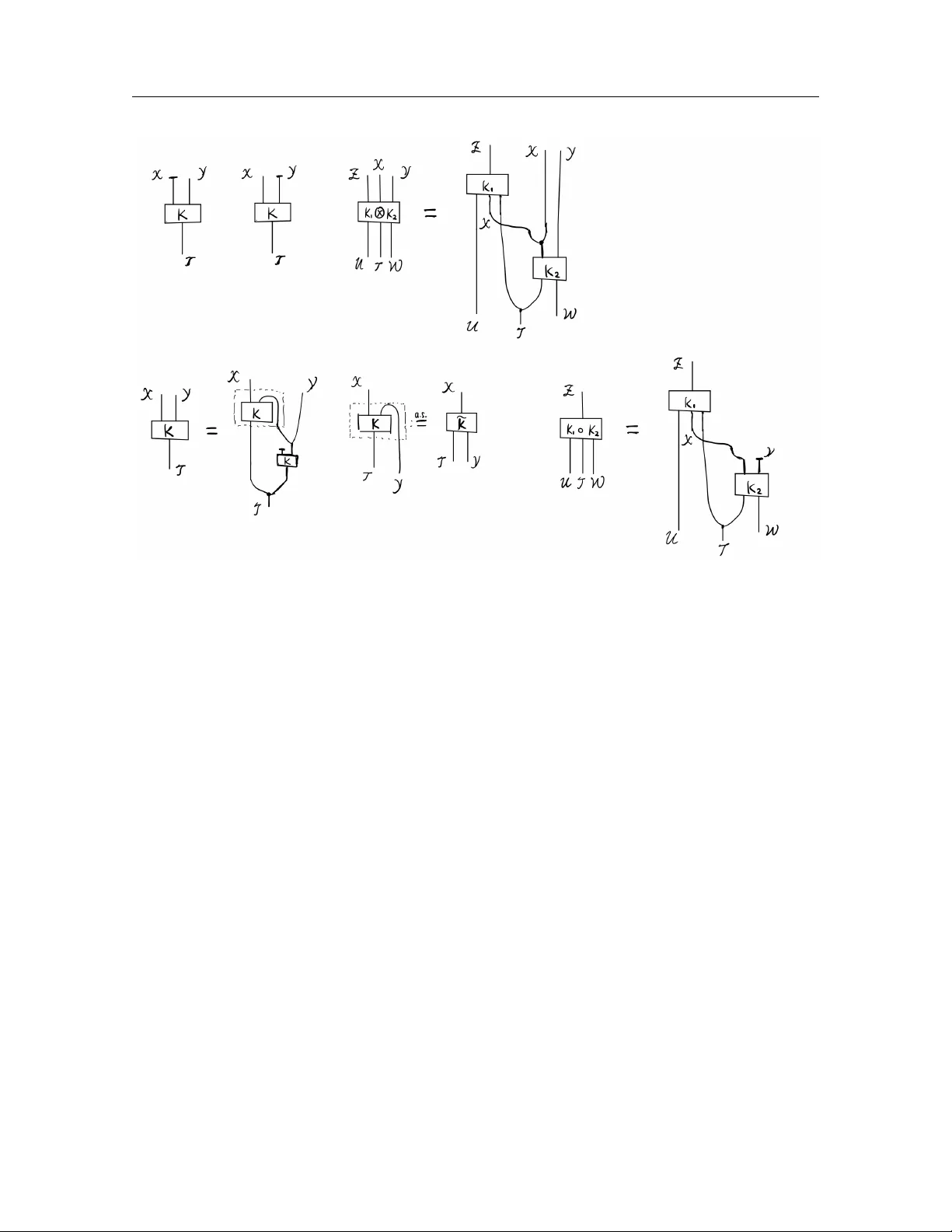
Recently, Forré (arXiv:2104.11547, 2021) introduced transitional conditional independence, a notion of conditional independence that provides a unified framework for both random and non-stochastic variables. The original paper establishes a strong gl…
Authors: Leihao Chen
Notes on F orr ´ e’s Notion of Conditional Indep endence and Causal Calculus for Con tin uous V ariables Leihao Chen ∗ Marc h 26, 2026 Abstract Recen tly , F orr ´ e (arXiv:2104.11547, 2021) introduced tr ansitional c onditional indep en- denc e , a notion of conditional indep endence that pro vides a unified framework for b oth random and non-stochastic v ariables. The original paper establishes a strong global Marko v prop ert y connecting transitional conditional indep endencies with suitable graphical sep- aration criteria for directed mixed graphs with input no des (iDMGs), together with a v ersion of causal calculus for iDMGs in a general measure-theoretic setting. These notes aim to further illustrate the motiv ations b ehind this framework and its connections to the literature, highlight certain subtlies in the general measure-theoretic causal calculus, and extend the “one-line” form ulation of the ID algorithm of Ric hardson et al. ( A nn. Statist. 51(1):334–361, 2023) to the general measure-theoretic setting. Con ten ts 1 Preliminaries 2 2 Motiv ating questions and examples 6 2.1 Causal calculus . . . . . . . . . . . . . . . . . . . . . . . . . . . . . . . . . . . . 6 2.2 Sufficiency , ancillarity and adequacy of statistics . . . . . . . . . . . . . . . . . 9 3 F orr ´ e’s approac h 9 3.1 F orr ´ e’s transitional conditional indep endence . . . . . . . . . . . . . . . . . . . 9 3.2 Causal identification results . . . . . . . . . . . . . . . . . . . . . . . . . . . . . 11 3.3 Concepts of statistics . . . . . . . . . . . . . . . . . . . . . . . . . . . . . . . . . 13 3.4 Wh y certain other approaches are unsatisfying . . . . . . . . . . . . . . . . . . 13 3.4.1 Using classic stochastic conditional independence . . . . . . . . . . . . . 13 3.4.2 Other approaches . . . . . . . . . . . . . . . . . . . . . . . . . . . . . . . 16 3.5 On the asymmetry of transitional conditional indep endence . . . . . . . . . . . 16 3.6 Relation to Da wid’s conditional indep endence for statistical operations . . . . . 19 ∗ K orteweg-de V ries Institute for Mathematics, Univ ersity of Amsterdam, Amsterdam, the Netherlands 1 1 Preliminaries 2 4 More on causal calculus for con tinuous v ariables 20 4.1 A positivity condition . . . . . . . . . . . . . . . . . . . . . . . . . . . . . . . . 21 4.2 A sufficien t condition for p oin twise iden tification . . . . . . . . . . . . . . . . . 21 5 An “one-line” formulation of measure-theoretic ID-algorithm using fixing op eration 26 6 Discussion 29 1 Preliminaries W e introduce some basic op erations on Marko v k ernels, the definition of Causal Bay esian Net work with late nt v ariables and input v ariables (L-iCBN), in terv entions on causal mo dels and graph manipulation for acyclic directed mixed graphs with input no des (iADMGs). References are [ 8 , 10 ]. Definition/Theorem 1.1 (Probabilit y calculus) . L et X , Y , Z , T , U , W b e standar d me asur able sp ac es. L et K( X , Y ∥ T ) : T 99K X × Y , K 1 ( Z ∥ U, X , T ) : U × X × T 99K Z , and K 2 ( X , Y ∥ T , W ) : T × W 99K X × Y b e Markov kernels. (1) Mar ginalization of Markov kernels: we define the mar ginal Markov kernels of K( X , Y ∥ T ) over X and Y , r esp e ctively, as fol lows: K( X ∥ T ) : T 99K X , K( X ∈ A ∥ T = t ) = K( X ∈ A, Y ∈ Y ∥ T = t ) , and K( Y ∥ T ) : T 99K Y , K( Y ∈ B ∥ T = t ) = K( X ∈ X , Y ∈ B ∥ T = t ) . (2) Pr o duct of Markov kernels: we define the pr o duct Markov kernel of K 1 and K 2 as fol lows: K 1 ( Z ∥ U, X , T ) ⊗ K 2 ( X , Y ∥ T , W ) : U × T × W 99K Z × X × Y , K 1 ( Z ∥ U, X , T ) ⊗ K 2 ( X , Y ∥ T , W ) ( B ; ( u, t, w )) = Z 1 B ( z , x, y ) K 1 ( Z ∈ d z ∥ U = u, X = x, T = t ) K 2 (( X , Y ) ∈ d( x, y ) ∥ T = t, W = w ) . (3) Disinte gr ation of Markov kernels: ther e exists a (essential ly unique) Markov kernel 1 (c al le d c onditional Markov kernel of K( X , Y ∥ T ) given Y ) e K ( X ∥ Y , T ) : Y × T 99K X such that K( X , Y ∥ T ) = e K( X ∥ Y , T ) ⊗ K( Y ∥ T ) , 1 The existence and (essential) uniqueness are guaranteed by [ 8 , Lemma 2.23 and Theorem 2.24] (see also [ 18 , Theorem 1.25] for a similar result). This generalizes the classical result of disintegration of probability distributions on standard measurable spaces to Marko v kernels. This result can also b e generalized to analytic measurable spaces [ 1 ] and universal measurable spaces [ 8 ]. 1 Preliminaries 3 wher e K( Y ∥ T ) is the mar ginal Markov kernel of K( X , Y ∥ T ) over Y . W e often denote e K ( X ∥ Y , T ) by K( X | Y ∥ T ) . Her e, essential uniqueness me ans that if Q( X ∥ Y , T ) is another Markov kernel, then we have K( X , Y ∥ T ) = Q( X ∥ Y , T ) ⊗ K( Y ∥ T ) iff the me asur able subset N ⊆ Y × T is a K( Y ∥ T ) -nul l set in Y × T , 2 wher e N : = { ( y , t ) ∈ Y × T | ∃ A ∈ Σ X s.t. Q( X ∈ A ∥ Y = y , T = t ) = K( X ∈ A | Y = y ∥ T = t ) } . Another commonly used op eration on Marko v kernels is the comp osition of Marko v k ernels K 1 ( Z ∥ U, X , T ) ◦ K 2 ( X , Y ∥ T , W ) : U × T × W 99K Z , whic h is defined using measurable sets B ⊆ Z via: K 1 ( Z ∥ U, X , T ) ◦ K 2 ( X , Y ∥ T , W ) ( B , ( u, t, w )) = Z K 1 ( Z ∈ B ∥ U = u, X = x, T = t ) K 2 ( X ∈ d x ∥ T = t, W = w ) , where Y is implicitly marginalized out. In fact, it can b e seen as a comp osition of the pro duct of Marko v kernels and marginalization of Marko v kernels. Remark 1.2 (String-diagrammatic representation of probabilit y calculus) . There is an intuitiv e string-diagrammatic representation of the probability calculus rules stated ab ov e, shown in Figure 1 , developed in the computer science and category theory literature [ 11 , 17 ]. As observ ed b y [ 11 ], w orking in the measu re-theoretic formulation is analogous to programming in mac hine co de, whereas the string-diagrammatic approac h is closer to a high-lev el programming language: it suppresses low-lev el details and emphasizes higher-level syn thetic structure. Interestingly , this level of abstraction suffices to prov e many classical results in measure-theoretic probability theory [ 2 , 11 – 13 ], and causal mo dels can lik ewise b e formulated at this lev el [ 14 , 21 ]. This viewp oint has sev eral adv an tages: (i) it yields an in tuitive comp ositional calculus for Mark ov kernels via string diagrams; (ii) a single abstract theorem can be instantiated in multiple concrete categories, including some not originally in tended for probabilit y , thereby pro ducing domain-sp ecific corollaries; and (iii) its syn thetic algebraic proofs suppress measure-theoretic tec hnicalities, making some argumen ts neater and more readily amenable to computer-assisted reasoning. Definition/Theorem 1.3 (Absolute con tinuit y and Do ob-Radon-Nik o dym deriv ativ e [ 8 , 10 ]) . L et K( W ∥ T ) and Q( W ∥ T ) b e two Markov kernels, and µ a σ -finite me asur e on W . W e say that K( W ∥ T ) is absolutely c ontinuous w.r.t. Q( W ∥ T ) if for al l t ∈ T and D ∈ Σ W Q( W ∈ D ∥ T = t ) = 0 = ⇒ K( W ∈ D ∥ T = t ) = 0 . In symb ols, we write K( W ∥ T ) ≪ Q( W ∥ T ) . The fol lowing two statements ar e e quivalent: (1) K( W ∥ T ) ≪ µ . (2) K( W ∥ T ) has a Do ob-R adon-Niko dym derivative w.r.t. µ , i.e., a joint measurable map: p : W × T → R ≥ 0 , ( w, t ) 7→ p ( w ∥ t ) , 2 N ⊆ Y × T is a K( Y ∥ T )-n ull set in Y × T if K( Y ∈ N t ∥ T = t ) = 0 for all t ∈ T where N t = { y ∈ Y | ( y , t ) ∈ N } . 1 Preliminaries 4 Figur e 1: String-diagr ammatic r epr esentation of the pr ob ability c alculus in Definition/The or em 1.1 . such that for al l t ∈ T and D ∈ Σ W : K( W ∈ D ∥ T = t ) = Z D p ( w ∥ t ) µ (d w ) . In this c ase, the Do ob-R adon-Niko dym derivative is essential ly unique, i.e., for two such derivatives p 1 and p 2 we have µ ( N t ) = 0 for al l t ∈ T wher e N : = { ( w , t ) ∈ W × T | p 1 ( w ∥ t ) = p 2 ( w ∥ t ) } ∈ Σ W ⊗ Σ T . F urthermor e, K( W ∥ T ) has a strictly p ositive Do ob-R adon-Niko dym derivative w.r.t. µ iff µ ≪ K( W ∥ T ) ≪ µ . Definition 1.4 (Causal Bay esian Netw ork) . A c ausal Bayesian network with latent no des and input no des (L-iCBN) M = D = ( I , V , L , E ) , P v ( X v ∥ X Pa D ( v ) ) v ∈V ˙ ∪ L is define d by: (1) a dir e cte d acyclic gr aph with latent no des and input no des (L-iDA G) D = ( I , V , L , E ) wher e I is the set of input no des, V is the set of observe d no des, and L is the set of latent no des; (2) for al l v ∈ I ˙ ∪ V ˙ ∪ L a standar d me asur able sp ac e X v ; (3) for every v ∈ V ˙ ∪ L , a Markov kernel P v ( X v ∥ X Pa D ( v ) ) fr om X Pa D ( v ) to X v . 1 Preliminaries 5 W e c al l the mar ginalize d acyclic dir e cte d mixe d gr aph with input no des, A = ( I , V , e E ) , the (induc e d) observable iADMG of M if A = D \L . W e c al l the Markov kernel P M ( X V ∥ X I ) : X I 99K X V the observable Markov kernel of M if P M ( X V ∈ · ∥ X I ) : = ≻ O v ∈V ˙ ∪ L P v ( X v ∥ X Pa D ( v ) ) ( · , X L ) , wher e ≺ is a top olo gic al or der on D , and ≻ denotes its r everse or der. Remark 1.5 (Input no des) . Input v ariables X I are also called “p olicy v ariables” [ 26 ] or “regime indicators” [ 7 ]. Definition 1.6 (Hard/soft manipulation on iADMGs) . L et A = ( I , V , E ) b e an iADMG and A ⊆ I ∪ V . W e define the har d manipulate d iADMG A do ( A ) = ( b I , b V , b E ) by • b I : = I ˙ ∪ ( A ∩ V ) ; • b V : = V \ A ; • b E : = E \ { b a | a ∈ A ∩ V and b a is in E } . W e define the soft manipulate d iADMG A do ( I A ) = ( e I , e V , e E ) by • e I : = I ˙ ∪ { I a } a ∈ A ∩V ; • e V : = V ; • e E : = E ˙ ∪ { I a a | a ∈ A ∩ V } . Note that hard manipulation, soft manipulation, and marginalization commute with eac h other: for A 1 , A 2 , B 1 , B 2 ⊆ V disjoin t, we hav e ( A do ( A 1 ) ) do ( A 2 ) = ( A do ( A 2 ) ) do ( A 1 ) = A do ( A 1 ∪ A 2 ) ( A do ( I B 1 ) ) do ( I B 2 ) = ( A do ( I B 2 ) ) do ( I B 1 ) = A do ( I B 1 ∪ B 2 ) ( A do ( A 1 ) ) do ( I B 1 ) = ( A do ( I B 1 ) ) do ( A 1 ) ( A do ( A 1 ) ) \L = ( A \L ) do ( A 1 ) and ( A do ( I B 1 ) ) \L = ( A \L ) do ( I B 1 ) . See [ 10 , Section 3] for a pro of. Definition 1.7 (Hard/soft interv ention on L-iCBN) . L et M = D = ( I , V , L , E ) , P v ( X v ∥ X Pa D ( v ) ) v ∈V ˙ ∪ L b e an L-iCBN and A ⊆ V . W e define har d intervene d L-iCBN M do ( A ) to b e M do ( A ) : = D do ( A ) , P v ( X v ∥ X Pa D ( v ) ) v ∈ ( V ˙ ∪ L ) \ A 2 Motiv ating questions and examples 6 and we have the interventional observable kernel: P M ( X V \ A ∥ X I , do ( X A )) : = P M do ( A ) ( X V \ A ∥ X I , X A ) . W e define soft intervene d L-iCBN M do ( I A ) to b e M do ( I A ) : = D do ( I A ) , e P v ( X v ∥ X Pa D do ( I A ) ( v ) ) v ∈V ˙ ∪ L wher e X I a : = X a ˙ ∪ { ⋆ } for a ∈ A and e P v ( X v ∥ X Pa D do ( I A ) ( v ) ) : = ( P v ( X v ∥ X Pa D ( v ) ) , if v / ∈ A Q v ( X v ∥ X Pa D ( v ) , X I v ) , if v ∈ A, and Q v ( X v ∈ · ∥ X Pa D ( v ) = x Pa D ( v ) , X I v = x I v ) : = ( P v ( X v ∈ · ∥ X Pa D ( v ) = x Pa D ( v ) ) , if x I v = ⋆ δ x I v ( · ) , if x I v = ⋆. 2 Motiv ating questions and examples In th is section, w e giv e t w o motiv ations (follo wing [ 8 ]) for in tro ducing transitional conditional indep endence: form ulating causal calculus in the general measure-theoretic setting and certain statistical concepts in terms of conditional independence. W e also give some examples and discussion of the subtleties in v olved. 2.1 Causal calculus Motiv ation 2.1. L et M = D = ( I , V , L , E ) , P v ( X v ∥ X Pa D ( v ) ) v ∈V ˙ ∪ L b e an iCBN and G : = D \L b e its mar ginalize d c ausal gr aph. L et A, B , C, D ⊆ V b e disjoint. Then we hop e to have the fol lowing rules in the gener al me asur e-the or etic setting: (1) If A ⊥ G do ( D ) B | C ∪ D , then we have P M ( X A | X B , X C ∥ do ( X D )) = P M ( X A | X C ∥ do ( X D )) . (2) If A ⊥ G do ( I B ,D ) I B | B ∪ C ∪ D , then we have P M ( X A | X C ∥ do ( X B , X D )) = P M ( X A | X B , X C ∥ do ( X D )) . (3) If A ⊥ G do ( I B ,D ) I B | C ∪ D , then we have P M ( X A | X C ∥ do ( X B , X D )) = P M ( X A | X C ∥ do ( X D )) . 2 Motiv ating questions and examples 7 F or an arbitrary iADMG G = ( I , V , E ) and A ⊆ V and B , C ⊆ I ∪ V , if w e hav e a global Mark ov prop ert y: A ⊥ G B | C = ⇒ X A ⊥ ⊥ X B | X C , then the abov e rules should follo w. Now the question reduces to: (i) finding the appropriate definition of the graphical separation rule ⊥ G and the conditional indep endence ⊥ ⊥ , and showing the corresp onding Mark ov prop erty; (ii) finding the conditions under which equality in an appropriate sense holds, which connects the tw o Marko v k ernels. One imp ortan t p oint is that X B and/or X C ma y b e non-sto c hastic v ariables, and therefore we need a new notion of conditional independence that can deal with non-sto c hastic v ariables prop erly . Note that classical sto chastic conditional indep endence and attempts to reduce the problem to the case of sto c hastic conditional indep endence are fallacious; see Section 3 . W e first presen t some examples to show the subtlet y behind p oin t (ii). Example 2.2 shows that the equalit y is not a point wise equality in general ev en if the causal calculus rules allo w us to iden tify a k ernel inv olving “do” in terms of a “do-free” k ernel. Example 2.3 sho ws that iden tification is v alid only if some appropriate p ositivit y condition holds. The issue of the p ositivit y condition ha ve already been iden tified in the literature (see, e.g., [ 10 , 19 ]), but their examples are about discrete v ariables and the example here in volv es contin uous v ariables. Example 2.2 (No p oin twise identification in general) . Consider a CBN M = D , P v ( X v ∥ X Pa D ( v ) ) where D is shown in Figure 2 and P a ( X a ) = Uni { [0 , 1] } and P b ( X b ∥ X a = x a ) = ( Uni { [0 , x a ] } , if x a ∈ [ 0 , 1] \ Q , δ x a , if x a ∈ [ 0 , 1] ∩ Q . Then we hav e the in terven tional k ernel P M ( X b ∥ do ( X a = x a )) = P b ( X b ∥ X a = x a ) . A version of the conditional distribution is P M ( X b | X a = x a ) = Uni { [0 , x a ] } . Note that for all x a ∈ Q ∩ (0 , 1] P M ( X b ∥ do ( X a = x a )) = P M ( X b | X a = x a ) . So, as w e can see, the iden tification result do es not hold point wise in general. a b D Figur e 2: Causal gr aph D of the CBN M in Example 2.2 . Example 2.3 (F ailure of back-door adjustment without appropriate p ositivit y condition) . Consider a CBN M = D , P v ( X v ∥ X Pa D ( v ) ) 2 Motiv ating questions and examples 8 c a b D Figur e 3: Causal gr aph D of the CBN M in Example 2.3 . where D is shown in Figure 3 and P c ( X c ) = Uni { [0 , 1] } P a ( X a ∥ X c = x c ) = P( 1 { x c ≥ 0 . 5 } U a ∥ X c = x c ) P b ( X b ∥ X a = x a , X c = x c ) = P( x a + x c U b ∥ X a = x a , X c = x c ) , where P( U a , U b ) = Uni { [0 , 1] } ⊗ Uni { [ − 0 . 5 , 0 . 5] } . The joint observ ational distribution is P M ( X a ∈ d x a , X b ∈ d x b , X c ∈ d x c ) = P b ( X b ∥ X a , X c ) ⊗ P a ( X a ∥ X c ) ⊗ P c ( X c ) (d x a , d x b , d x c ) = 1 x c δ 0 (d x a ) 1 {− 0 . 5 x c ≤ x b ≤ 0 . 5 x c } 1 { 0 < x c < 0 . 5 } d x b d x c + 1 x c 1 { 0 ≤ x a ≤ 1 } 1 { x a − 0 . 5 x c ≤ x b ≤ x a + 0 . 5 x c } 1 { 0 . 5 ≤ x c ≤ 1 } d x a d x b d x c . One choice of the conditional distribution of X b giv en X a and X c is P M ( X b ∈ d x b | X a = x a , X c = x c ) = 1 x c 1 {− 0 . 5 x c ≤ x b ≤ 0 . 5 x c } 1 { 0 < x c < 0 . 5 } d x b + 1 { x c = 0 } δ 0 (d x b ) + 1 x c 1 { x a − 0 . 5 x c ≤ x b ≤ x a + 0 . 5 x c } 1 { 0 . 5 ≤ x c ≤ 1 } d x b F rom M , we can compute the interv entional k ernel P M ( X b ∈ d x b ∥ do ( X a = x a )) = P b ( X b ∈ d x b ∥ X a = x a , X c ) ⊗ P c ( X c ) = − log (2 | x b − x a | ) 1 { 2 | x b − x a | ≤ 1 } d x b . Note that P M ( X b ∈ d x b | X a = x a , X c ) ◦ P M ( X c ) = − log (2 | x b − x a | ) 1 { 0 . 5 ≤ 2 | x b − x a | ≤ 1 } d x b + log (2) 1 { 2 | x b − x a | < 0 . 5 } d x b − log (4 | x b | ) 1 { 2 | x b | < 0 . 5 } d x b . So, for al l x a ∈ (0 , 1], P M ( X b ∥ do ( X a = x a )) = P M ( X b | X a = x a , X c ) ◦ P M ( X c ) . This sho ws that the form ulation of the tw o rules in Motiv ation 2.1 should b e upgraded to that if certain graphical separation holds, then under certain positivity assumptions, the Mark ov k ernel on the left is equal to the one on the right up to some p oin ts (hop efully) in a small set. W e return to p oin t (ii) in Sections 3.2 and 4 . 3 F orr´ e’s approac h 9 2.2 Sufficiency , ancillarit y and adequacy of statistics Motiv ation 2.4. Sufficiency, ancil larity and ade quacy of statistics should admit a formulation in terms of c onditional indep endenc e. L et { P( X , Y ∥ ϑ = θ ) } θ ∈ Θ b e a statistic al mo dels. L et S b e a statistic of X . Then we have (1) S is an ancil lary statistic of X w.r.t. ϑ iff S ⊥ ⊥ ϑ . (2) S is a sufficient statistic of X w.r.t. ϑ iff X ⊥ ⊥ ϑ | S . (3) S is an ade quate statistic of X for Y w.r.t. ϑ iff X ⊥ ⊥ ϑ, Y | S . 3 F orr ´ e’s approac h W e discuss F orr´ e’s approach to addressing the problems raised in Motiv ations 2.1 and 2.4 . Its theoretical foundation is giv en by transitional conditional indep endence and the associated Mark ov prop ert y . After explaining ho w these problems are resolved within this framew ork, w e briefly discuss wh y certain alternativ e approaches fail to achiev e the desired goals. Finally , w e commen t on the asymmetric nature of transitional conditional indep endence and its connections to Dawid’s notion of conditional indep endence for statistical op erations. 3.1 F orr ´ e’s transitional conditional indep endence The conten t of this subsection is based on [ 8 , 10 ]. First, recall that w e wan t a notion of conditional independence that can deal with Moti- v ations 2.1 and 2.4 , whic h accommo date both sto c hastic and non-sto c hastic v ariables. Let X : W → X b e a rand om v ariable defined on probabilit y space ( W , Σ W , P( W )) and ϑ : T → Θ a non-sto c hastic v ariable defined on measurable space ( T , Σ T ). Then we can define (1) X ∗ : ( W × T , Σ W ⊗ Σ T ) → X as X ∗ ( w , t ) = X ( w ), and (2) ϑ ∗ : ( W × T , Σ W ⊗ Σ T ) → Θ as ϑ ∗ ( w , t ) = ϑ ( t ). Hence, it is conv enien t to w ork in the follo wing ground framew ork [ 8 ]. Definition 3.1 (T ransitional probability space and transitional random v ariable) . L et K( W ∥ T ) b e a Markov kernel fr om ( T , Σ T ) to ( W , Σ W ) . Then we c al l the tuple ( W × T , Σ W ⊗ Σ T , K( W ∥ T )) a tr ansitional pr ob ability sp ac e . A me asur able map X : W × T → X is c al le d a tr ansitional r andom variable . This generalizes the the notions of probabilit y space, random v ariable, and non-sto c hastic v ariable. If T = { ⋆ } , then ( W × T , K( W ∥ T )) is a probability space and X is a random v ariable. If W = { ⋆ } , then X is a non-stochastic v ariable. One can consider a transitional random v ariable as a family of random v ariables (measurably) parameterized by t ∈ T . F or t ∈ T w e define the measurable map: X t : W → X , w 7→ X t ( w ) : = X ( w , t ) , whic h can b e considered a random v ariable on the probability space ( W , K( W ∥ T = t )). No w w e can state the definition of F orr´ e’s trans itional conditional independence [ 8 , Defini- tion 3.1]. 3 F orr´ e’s approac h 10 Definition 3.2 (T ransitional conditional indep endence) . L et ( W × T , K( W ∥ T )) b e a tr ansi- tional pr ob ability sp ac e. Consider tr ansitional r andom variables: X : W × T → X , Y : W × T → Y , Z : W × T → Z . W e say that X is c onditional ly indep endent of Y given Z w.r.t. K( W ∥ T ) , in symb ols: X F ⊥ ⊥ K( W ∥ T ) Y | Z , if ther e exists a Markov kernel Q( X ∥ Z ) : Z 99K X , such that: K( X , Y , Z ∥ T ) = Q( X ∥ Z ) ⊗ K( Y , Z ∥ T ) , wher e K( Y , Z ∥ T ) is the mar ginal of K( X , Y , Z ∥ T ) . A s a sp e cial c ase, we define: X F ⊥ ⊥ K( W ∥ T ) Y : ⇐ ⇒ X F ⊥ ⊥ K( W ∥ T ) Y | ∗ . This notion of conditional indep endence admits a natural generalization to Mark ov cate- gories via its elegant factorization-based definition [ 14 , Definition 16]. Remark 3.3 (Essen tial uniqueness) . The Mark ov kernel Q( X ∥ Z ) appearing in the conditional indep endence X F ⊥ ⊥ K( W ∥ T ) Y | Z in definition 3.2 is then a version of a conditional Marko v k ernel K( X | Y , Z ∥ T ) and is th us essen tially unique in the sense that for every measurable subset A ⊆ X , the set N A := { ( t, y , z ) ∈ T × Y × Z | K( X ∈ A | Y = y , Z = z ∥ T = t ) = Q( X ∈ A ∥ Z = z ) } is a measurable K( Y , Z ∥ T )-null set. Definition 3.4 (Graphical separation) . L et G = ( I , V , E ) b e an iADMG. L et A, B , C ⊆ I ∪ V b e (not ne c essarily disjoint) subsets of no des. W e then say that A is id -sep ar ate d fr om B given C in G , in symb ols: A id ⊥ G B | C, if every p ath fr om a no de in A to a no de in B ∪ I is d -blo cke d by C (b eing d -blo cke d is ac c or ding to the usual definition of d -sep ar ation in the liter atur e [ 23 , 24 ]). Theorem 3.5 (Asymmetric separoid rules [ 8 , Theorems 3.1, 5.11]) . The tr ansitional c onditional indep endenc e (Definition 3.2 ) and the gr aphic al sep ar ation rule (Definition 3.4 ) b oth satisfy the asymmetric sep ar oid rules. Theorem 3.6 (Strong global Mark ov prop ert y [ 8 , Theorem 6.3]) . L et M = D = ( I , V , L , E ) , P v ( X v ∥ X Pa D ( v ) ) v ∈V ˙ ∪ L b e an L-iCBN and A, B , C ⊆ I ∪ V . Set A : = D \L . Then we have A id ⊥ A B | C = ⇒ X A F ⊥ ⊥ P M ( X V ∥ X I ) X B | X C . 3 F orr´ e’s approac h 11 3.2 Causal iden tification results F rom Theorem 3.6 , one can pro ve the following version of causal calculus in the general measure-theoretic setting [ 8 , 10 ]. Theorem 3.7 (Causal calculus (ADMGs)) . L et M = D = ( V , L , E ) , P v ( X v ∥ X Pa D ( v ) ) v ∈V ˙ ∪ L b e an L-CBN, and let A : = D \L b e the observational ADMG of M . L et A, B , C, D ⊆ V b e disjoint. A ssume that ther e ar e σ -finite r efer enc e me asur es µ v on X v for e ach v ∈ V (write µ F : = N v ∈ F µ v for F ⊆ V ). (1) Insertion/deletion of observation: Supp ose A id ⊥ A do ( D ) B | C ∪ D . Then ther e exists a unique Markov kernel Q( X A ∥ X C , X D ) , up to a me asur able P M ( X C ∥ do ( X D )) -nul l set in X C ∪ D , which is a version of P M ( X A | X B 1 , X C ∥ do ( X D )) for every B 1 ⊆ B simultane ously. If µ B ∪ C ≪ P M ( X B , X C ∥ do ( X D )) ≪ µ B ∪ C , then e quality holds P M ( X A | X B = x B , X C = x C ∥ do ( X D = x D )) = P M ( X A | X C = x C ∥ do ( X D = x D )) for al l ( x B , x C , x D ) ∈ ( X B × X C × X D ) \ N wher e N ⊆ X B ∪ C ∪ D is a me asur able set such that µ B ∪ C ( N x D ) = 0 for al l x D ∈ X D . Her e, e quality me ans e quality as pr ob ability me asur es on X A . (2) A ction/observation exchange: Supp ose A id ⊥ A do ( I B ,D ) I B | B ∪ C ∪ D . Then ther e exists a unique Markov kernel Q( X A ∥ X B , X C , X D ) , up to a me asur able P M ( X B , X C ∥ do ( X I B , X D )) - nul l set N ⊆ X B ∪ C ∪ D , 3 which is a version of P M ( X A | X B 1 , X C ∥ do ( X B 2 , X D )) for every de c omp osition B = B 1 ˙ ∪ B 2 simultane ously. If µ B ∪ C ≪ P M ( X B , X C ∥ do ( X D )) ≪ µ B ∪ C and µ C ≪ P M ( X C ∥ do ( X B , X D )) ≪ µ C , then the e quality holds P M ( X A | X C = x C ∥ do ( X B = x B , X D = x D )) = P M ( X A | X B = x B , X C = x C ∥ do ( X D = x D )) for al l ( x B , x C , x D ) ∈ ( X B × X C × X D ) \ e N wher e e N ⊆ X B ∪ C ∪ D is a me asur able set such that µ B ∪ C ( e N x D ) = 0 for al l x D ∈ X D . Her e, e quality me ans e quality as pr ob ability me asur es on X A . (3) Insertion/observation of action: Supp ose A id ⊥ A do ( I B ,D ) I B | C ∪ D . Then ther e exists a unique Markov kernel Q( X A ∥ X C , X D ) , up to a me asur able P M ( X C ∥ do ( X I B , X D )) - nul l set N × X I B ⊆ X C ∪ D × X I B , which is a version of P M ( X A | X C ∥ do ( X B 2 , X D )) for every B 2 ⊆ B simultane ously. If µ C ≪ P M ( X C ∥ do ( X B , X D )) ≪ µ C and µ C ≪ P M ( X C ∥ do ( X D )) ≪ µ C , then the e quality holds P M ( X A | X C = x C ∥ do ( X B = x B , X D = x D )) = P M ( X A | X C = x C ∥ do ( X D = x D )) for al l ( x B , x C , x D ) ∈ ( X B × X C × X D ) \ ( X B × e N ) wher e e N ⊆ X C ∪ D is a me asur able set such that µ C ( e N x D ) = 0 for al l x D ∈ X D . Her e, e quality me ans e quality as pr ob ability me asur es on X A . 3 It means that N is a P M ( X B 1 , X C ∥ do ( X B 2 , X D ))-n ull set for every decomp osition B = B 1 ˙ ∪ B 2 sim ulta- neously . 3 F orr´ e’s approac h 12 c u b a G ( M ) Figur e 4: Causal gr aph D of the CBN M in Example 3.11 . Remark 3.8 (On the absolute contin uit y condition (p ositivit y condition)) . (1) WLOG, we can take the σ -finite reference measure µ to b e a probabilit y measure. (2) A Mark o v k ernel K( X ∥ T ) has a strictly p ositiv e Do ob-Radon-Nik o dym deriv ative w.r.t. σ -finite measure µ on X iff µ ≪ K( X ∥ T ) ≪ µ . If X = T = R and µ = λ , then µ ≪ K( X ∥ T ) ≪ µ states that K( X ∈ d x ∥ T = t ) = k ( x ∥ t )d x for some strictly p ositiv e densit y function k ( x ∥ t ) that is join tly measurable w.r.t. x and t . In the discrete case, this is equiv alent to sa ying that k ( x ∥ t ) > 0 for all x ∈ X and t ∈ T , where k ( · ∥ · ) is the probabilit y mass function of K( X ∥ T ). See, e.g., [ 10 , Corollary 2.3.20]. Prop osition 3.9 (Back-door adjustment [ 10 , Corollary 5.2.6]) . Under the setting of The o- r em 3.7 , let F ⊆ V . A ssume F id ⊥ A do ( I B ) I B , A id ⊥ A do ( I B ) I B | B ∪ F , and P M ( X F ) ⊗ P M ( X B ) ≪ P M ( X F , X B ) . Then the fol lowing adjustment formulas hold: P M ( X A , X F ∥ do ( X B )) = P M ( X A | X F , X B ) ⊗ P M ( X F ) P M ( X B ) -a.s., P M ( X A ∥ do ( X B )) = P M ( X A | X F , X B ) ◦ P M ( X F ) P M ( X B ) -a.s. Remark 3.10. In Example 2.3 , the p ositivity condition P M ( X c ) ⊗ P M ( X b ) ≪ P M ( X c , X b ) is violated. The following example shows that the positivity conditions in Theorem 3.7 are only sufficien t, but not necessary in general. Example 3.11 (P ositivity condition in Theorem 3.7 is not necessary) . Consider an L-CBN M = D , P v ( X v ∥ X Pa D ( v ) ) where D is shown in Figure 4 and P u ( X u ) = Uni { [0 , 1] } P b ( X b ∥ X u = x u ) = N ( x u , 1) P c ( X c ∥ X u = x u , X b = x b ) = δ x u x b P a ( X a ∥ X c = x c ) = N ( x c , 1) . A conditional densit y f M ( x a | x b , x c ) is f M ( x a | x b , x c ) = 1 √ 2 π exp − ( x a − x c ) 2 2 ! . 3 F orr´ e’s approac h 13 F rom M , we can compute that a conditional in terven tional density f M ( x a | x c ∥ do ( x b )) is f M ( x a | x c ∥ do ( x b )) = 1 √ 2 π exp − ( x a − x c ) 2 2 ! , whic h is equal to f M ( x a | x b , x c ). Hence, we ha ve the identification result that P M ( X a | X c = x c ∥ do ( X b = x b )) = P M ( X a | X c = x c , X b = x b ) for all ( x b , x c ) ∈ R 2 \ N , where N is a λ 2 -n ull set in R 2 . Ho wev er, the p ositivit y condition in the second rule of causal calculus (Theorem 3.7 ) is violated. Indeed, w e ha v e that P M ( X c ∥ do ( X b = x b )) = Uni { [0 , x b ] } , if x b > 0 , Uni { [ x b , 0] } , if x b < 0 , δ 0 , if x b = 0 , whic h does not p ossess a strictly p ositiv e densit y w.r.t. λ for all x b . 3.3 Concepts of statistics Let X : W × Θ → X b e a transitional random v ariable and S : X → S a measurable function (statistics), which can b e considered as a transitional random v ariable via S : W × Θ → S , ( w , θ ) 7→ S ( X ( w , θ )) . Using transitional conditional indep endence, we can express the fact that S is a sufficient statistic of X w.r.t. ϑ as X F ⊥ ⊥ P( W ∥ ϑ ) ϑ | S. Ancillary statistic and adequate statistic can b e tackled similarly . See [ 8 ] for more details. 3.4 Wh y certain other approaches are unsatisfying In [ 8 ], comparisons b et w een transitional conditional indep endence and other notions of con- ditional indep endence are presen ted. How ever, some arguments and claims are to o brief to fully explain wh y alternative approac hes fall short, p oten tially lea ving readers uncertain ab out the justification for the proposed framework. This subsection, therefore, aims to provide a more detailed analysis of why certain alternativ e approaches fail to satisfy the requirements outlined in Motiv ations 2.1 and 2.4 . A natural first approac h is to reduce the problem to the domain of purely sto c hastic conditional indep endence. W e in tro duce tw o such notions and demonstrate ho w they either fail outright or provide weak er solutions to the issues raised in Motiv ations 2.1 and 2.4 . 3.4.1 Using classic sto c hastic conditional indep endence Definition 3.12. L et us define a c onditional indep endenc e as fol lows: X s ⊥ ⊥ Y | Z ⇐ ⇒ ∀ t ∈ T , X t ⊥ ⊥ P( X,Y ,Z ∥ T = t ) Y t | Z t , wher e X t ( w ) = X ( w , t ) , Y t ( w ) = Y ( w , t ) , and Z t ( w ) = Z ( w , t ) and P( X , Y , Z ∥ T = t ) = ( X t , Y t , Z t ) ∗ P( W ∥ T = t ) . 3 F orr´ e’s approac h 14 This notion is not suitable for expressing sufficien t statistics and casual calculus. If Y is a non-sto c hastic v ariable, then Y t is a constan t and for all t ∈ T w e alw ays ha ve X t ⊥ ⊥ P( X,Y ,Z ∥ T = t ) Y t | Z t , whic h implies that X s ⊥ ⊥ Y | Z alw ays hold. Therefore, all the statistics are sufficient and causal calculus rules are alwa ys applicable according to this notion, whic h is of course not the case. No w, w e consider another approach of putting probabilit y distributions on non-stochastic v ariables. Definition 3.13. L et us define a c onditional indep endenc e as fol lows [ 9 ]: X FM ⊥ ⊥ Y | Z ⇐ ⇒ ∀ Q( T ) ∈ P ( T ) , X ⊥ ⊥ P( X,Y ,Z ) Y | Z , wher e P( X, Y , Z ) : = ( X , Y , Z ) ∗ (P( W ) ⊗ Q( T )) . Can w e say that S is a sufficien t statistic of X iff X FM ⊥ ⊥ ϑ | S ? No in general, this condition is equiv alent to that S is a p airwise sufficient statistic of X [ 5 ], i.e., for ev ery pair { P θ 1 ( X ) , P θ 2 ( X ) } ⊆ { P θ ( X ) } θ there exists a Marko v kernel Q( X ∥ S ) suc h that P( X | S ∥ ϑ = θ 1 ) = Q( X ∥ S ) , P( S ∥ ϑ = θ 1 )-a.s., P( X | S ∥ ϑ = θ 2 ) = Q( X ∥ S ) , P( S ∥ ϑ = θ 2 )-a.s. If the model { P θ ( X ) } θ ∈ Θ is dominated, then we ha ve Sufficiency ⇐ ⇒ P airwise Sufficiency , but in general we ha ve Sufficiency ⇐ = = ⇒ P airwise Sufficiency . This approach do es not give the strongest causal calculus in terms of n ull sets. F or illustration, we consider the third rule of causal calculus. Assume that a reference measure µ C is such that the p ositivit y condition holds and X A FM ⊥ ⊥ X I B | X C , X D . Since P Q ( X A , X I B , X D | X C ) = P M ( X A | X C ∥ do ( X I B ) , do ( X D )) ⊗ Q( X I B , X D ) µ C -a.s. , conditioning on X I B and X D giv es P M ( X A | X C ∥ do ( X I B ) , do ( X D )) = P Q ( X A | X C , X I B , X D ) µ C ⊗ Q( X I B , X D )-a.s. = P Q ( X A | X C , X D ) P Q ( X C , X I B , X D )-a.s. = P M ( X A | X C ∥ do ( X D )) µ C ⊗ Q( X D )-a.s. 3 F orr´ e’s approac h 15 F rom this, one can at most conclude that for every fixed ( x B , x D ) ∈ X B × X D , there exists a µ C -n ull set N x B ,x D ⊆ X C suc h that for every x C / ∈ N x B ,x D P M ( X A | X C = x C ∥ do ( X B = x B ) , do ( X D = x D )) = P M ( X A | X C = x C ∥ do ( X D = x D )) . This is w eak er than that for ev ery fixed x D ∈ X D there exists a single null set N x D ⊆ X C suc h that for all x B ∈ X B and all x C ∈ X C \ N x D the equality b et w een the t wo k ernels holds. F or illustration, we presen t one concrete example in Example 3.14 . Example 3.14 (Wh y a common µ C -n ull set in X C need not exist) . The stronger conclusion with a single µ C -n ull set in X C do es not hold in general. Let X C = X B = [0 , 1] , µ C = λ | [0 , 1] , where λ denotes Leb esgue measure. F or simplicit y , we assume D = ∅ . Note that this already co vers the stronger claim, since it corresp onds to the case of a single fixed x D . Let the target space b e { 0 , 1 } , and define tw o Marko v k ernels K 1 , K 2 : X C × X B 99K { 0 , 1 } b y K 1 ( · ∥ x C , x B ) = ( δ 1 , x C = x B , δ 0 , x C = x B , K 2 ( · ∥ x C , x B ) = δ 0 . Let D : = { ( x C , x B ) ∈ [ 0 , 1] 2 | x C = x B } b e the diagonal, i.e. the set on which K 1 and K 2 differ. Then for every probabilit y measure Q ∈ P ([0 , 1]), ( µ C ⊗ Q)( D ) = Z [0 , 1] µ C ( { x B } ) Q(d x B ) = 0 . Hence K 1 ( · ∥ x C , x B ) = K 2 ( · ∥ x C , x B ) ( µ C ⊗ Q)-a.s. on X C × X B for every probabilit y measure Q ∈ P ([ 0 , 1]). Moreov er, for eac h fixed x B ∈ [ 0 , 1], K 1 ( · ∥ x C , x B ) = K 2 ( · ∥ x C , x B ) for all x C ∈ [ 0 , 1] \ N x B , where N x B = { x B } , which is a µ C -n ull set. Note that S x B ∈ [0 , 1] N x B = [0 , 1]. In fact, there is no single µ C -n ull set N ⊆ [0 , 1] such that K 1 ( · ∥ x C , x B ) = K 2 ( · ∥ x C , x B ) for all ( x C , x B ) ∈ ([ 0 , 1] \ N ) × [ 0 , 1] . T o see that, assume on the contrary that suc h null set N exists. If x C ∈ [0 , 1] \ N , choose x B = x C . Therefore, K 1 ( { 1 } ∥ x C , x B ) = 1 = 0 = K 2 ( { 1 } ∥ x C , x B ) . This causes a con tradiction. Hence, although for eac h fixed x B the equality holds outside a µ C -n ull set in X C , one cannot in general c ho ose this n ull set uniformly in x B . 3 F orr´ e’s approac h 16 W e no w present the connections among those three notions of conditional indep endence. It is sho wn in [ 8 , 9 ] that X F ⊥ ⊥ K( W ∥ T ) Y | Z , T ⇐ ⇒ X s ⊥ ⊥ Y | Z , and that if T is discrete or { P( X , Y , Z | T = t ) } t ∈T is dominated, then X F ⊥ ⊥ Y | Z ⇐ ⇒ X FM ⊥ ⊥ Y | Z, and in general X F ⊥ ⊥ Y | Z ⇐ = = ⇒ X FM ⊥ ⊥ Y | Z. 3.4.2 Other approac hes A notion of conditional indep endence for sto c hastic and non-stochastic v ariables is prop osed in [ 25 ]. How ev er, it is only defined in the discrete setting and not in the general measure- theoretic setting. F urthermore, there is no discussion of the problems p osed in Motiv ations 2.1 and 2.4 . The extended conditional independence prop osed in [ 3 ] is compared with the transitional conditional indep endence in [ 8 ]. Therefore, we will not discuss those notions of conditional indep endence proposed in [ 3 , 25 ]. W e shall discuss further the relation b et ween the conditional independence for statistical operations prop osed in [ 5 ] and the transitional conditional independence in the next subsection, which is missing in the original paper [ 8 ]. Ho wev er, note that the application of the CI for statistical op erations on graphical mo dels and causal calculus is not discussed in [ 5 ]. 3.5 On the asymmetry of transitional conditional indep endence F rom Definition 3.2 , it is easy to see that transitional conditional indep endence is asymmetric, i.e., X F ⊥ ⊥ K( W ∥ T ) Y | Z = ⇒ Y F ⊥ ⊥ K( W ∥ T ) X | Z . W e can symmetrize it if w e wan t a symmetrized notion of conditional indep endence [ 8 , Section L.6]. Definition 3.15 (Symmetric version of transitional conditional independence) . Inde e d, we c an define X ∨ ⊥ ⊥ K( W ∥ T ) Y | Z by X F ⊥ ⊥ K( W ∥ T ) Y | Z ∨ Y F ⊥ ⊥ K( W ∥ T ) X | Z . It is easy to see that the symmetric version is indeed symmetric and the transitional conditional indep endence is, in general, strictly stronger than its symmetrized v ersion: X F ⊥ ⊥ K( W ∥ T ) Y | Z ⇐ = = ⇒ X ∨ ⊥ ⊥ K( W ∥ T ) Y | Z . 3 F orr´ e’s approac h 17 If desired, then it is possible to work with the symmetric v ersion (Definition 3.15 ). First, note that in the setting of Motiv ations 2.1 and 2.4 , w e hav e X I B F ⊥ ⊥ P M ( X V ∥ do ( X D )) X A | X B , X C , X D , X I B F ⊥ ⊥ P M ( X V ∥ do ( X D )) X A | X C , X D and ϑ F ⊥ ⊥ P( W ∥ ϑ ) X | S. So we ha ve X A F ⊥ ⊥ K( W ∥ T ) X I B | X B , X C , X D ⇐ ⇒ X A ∨ ⊥ ⊥ K( W ∥ T ) X I B | X B , X C , X D X A F ⊥ ⊥ K( W ∥ T ) X I B | X B , X C , X D ⇐ ⇒ X A ∨ ⊥ ⊥ K( W ∥ T ) X I B | X B , X C , X D X F ⊥ ⊥ P( X W ∥ ϑ ) ϑ | S ⇐ ⇒ X ∨ ⊥ ⊥ P( X W ∥ ϑ ) ϑ | S. Ho wev er, conditional independence is, at its core, a notion of irr elevanc e . The statement that X is conditionally indep enden t of Y giv en Z is in terpreted as saying that, once Z is kno wn, Y is irrelev ant for X . In this sense, the concept is inherently asymmetric; the symmetry of ordinary sto c hastic conditional independence is a sp ecial feature of that particular setting. See, for example, the discussions in [ 4 – 6 ]. T o gain further intuition for the asymmetry of transitional conditional independence, it is helpful to consider the string-diagrammatic represen tation giv en in [ 14 , Definition 16 and Remark 17]. Recall that the conditional indep endence X F ⊥ ⊥ K( W | T ) Y | Z means that there exists a k ernel Q( X ∥ Z ) such that K( X , Y , Z ∥ T ) = Q( X ∥ Z ) ⊗ K( Y , Z ∥ T ) = Q( X ∥ Z ) ⊗ K( Y | Z ∥ T ) ⊗ K( Z ∥ T ) . W rite K 0 : = K( Y , Z ∥ T ) , K 1 : = K( Y | Z ∥ T ) , K 2 : = K( Z ∥ T ) . The corresp onding string diagram is sho wn in Figure 5 . F rom this representation, the asymmetry b ecomes more transparen t: the v ariable X can b e generated from the information in Z alone via the k ernel Q( X ∥ Z ), whereas Z need not suffice to generate Y . Indeed, Y ma y still dep end on information contained in T that is not captured b y Z . Also note that the symmetric v ersion in whic h Q can also depend on T in Figure 5 is not strong enough to pro ve Theorem 28 in [ 14 ] as argued in [ 14 , Remark 17]. T o reinforce the intuition and clarify the claim that the symmetrized v ersion might ha ve lost some information ab out the in terplay b et w een X , Y , Z and T , we consider an example in the setting of causal models. Consider an iCBN M = ( D = ( I , V , E ) , { P v } v ) with I : = { I v : v ∈ V } . 3 F orr´ e’s approac h 18 Figur e 5: String-diagr ammatic r epr esentation of tr ansitional c onditional indep endenc e. a c b I a I c I b D a c b I a I c I b e D Figur e 6: Causal gr aph D in which a id ⊥ D b | c ∪ I a but b id ⊥ D a | c ∪ I a , and c ausal gr aph e D in which b id ⊥ D a | c ∪ I a . The graph D is given in Figure 6 . W e assume that, for D and P M ( X V ∥ X I ), a transi- tional conditional independence holds (Definition 3.2 ) iff a corresponding id -separation holds (Definition 3.4 ). The conditional independence X a F ⊥ ⊥ P M ( X V | X I ) X b | X c , X I a implies that there exists a Mark ov k ernel Q( X a ∥ X c , X I a ) such that P M ( X a , X b , X c ∥ X I ) = Q( X a ∥ X c , X I a ) ⊗ P M ( X b , X c ∥ X I ) . By the construction of the causal mo del, this Mark ov k ernel can indeed b e c hosen as Q( X a ∥ X c , X I a ) = P a ( X a ∥ X Pa D ( a ) ) . In contrast, the conditional indep endence X b F ⊥ ⊥ P M ( X V | X I ) X a | X c , X I a do es not hold. Indeed, if it did, then there w ould exist a Mark o v k ernel e Q ( X b ∥ X c , X I a ) such that P M ( X a , X b , X c ∥ X I ) = e Q( X b ∥ X c , X I a ) ⊗ P M ( X a , X c ∥ X I ) . 3 F orr´ e’s approac h 19 Ho wev er, from the construction of the causal mo del, it is not clear how suc h a k ernel could arise. T o see this more concretely , assume that all relev ant Marko v kernels admit densities with resp ect to suitable reference measures. Then p ( x a , x b , x c ∥ x I ) = q ( x a ∥ x c , x I a ) p ( x b , x c ∥ x I ) = q ( x a ∥ x c , x I a ) p ( x b ∥ x c , x I ) p ( x c ∥ x I ) = p ( x b ∥ x c , x I ) q ( x a ∥ x c , x I a ) p ( x c ∥ x I ) = p ( x b ∥ x c , x I ) p ( x a , x c ∥ x I ) . Th us, the reverse conditional indep endence would require X b to b e generated by a kernel dep ending only on X c and X I a . But from the construction of the causal mo del, we kno w that X b dep ends on X I b , and hence in general on information contained in X I b ey ond X c and X I a . Therefore, one cannot conclude that X b dep ends only on X c and X I a . F or suc h a reverse conditional independence to hold, the causal model w ould need to ha ve a fundamentally differen t structure. One such example, denoted b y e D , is sho wn in Figure 6 . 3.6 Relation to Dawid’s conditional indep endence for statistical op erations In [ 5 ], Da wid introduced a notion of conditional independence for statistical op erations. W e only consider standard measurable spaces. Definition 3.16 (Statistical Op eration) . A map Π : L ∞ ( F , N F ) → L ∞ ( G , N G ) satisfying (P1)-(P4) is terme d a statistic al op er ation (SO) over ( F , N F ) given ( G , N G ) , wher e F and G ar e σ -algebr as and N F and N G ar e σ -ide als. (P1) (Line arity): Π( a 1 f 1 + a 2 f 2 ) = a 1 Π f 1 + a 2 Π f 2 , for a 1 , a 2 ∈ R and f 1 , f 2 ∈ L ∞ ( F , N F ) ; (P2) (Positivity): f ≥ 0 = ⇒ Π f ≥ 0 ; (P3) (Normalization): Π 1 = 1 , wher e 1 denotes the c onstant 1 function; (P4) (Continuity): If ( f n ) ∞ n =1 is a c ountable se quenc e that de cr e ases monotonic al ly to 0 , then inf n Π f n = 0 . Definition 3.17 (Conditional indep endence for SO) . L et Π b e a statistic al op er ation over ( F , N F ) given ( G , N G ) . Supp ose that A is a σ -sub algebr a of F , and B and C ar e σ -sub algebr as of G satisfying B ∨ C = G . W e say that A is indep endent of B given C (w.r.t. Π ), and write A D ⊥ ⊥ B | C [Π] if for al l f ∈ L ∞ ( A ) , ther e exists a version of Π f that is C -me asur able. Note that the conditional indep endence for SO is also asymmetric. W e can formulate sufficien t statistics in terms of conditional independence for statistical operations. Example 3.18 (Sufficient statistics) . Define F : = σ ( X ) and G : = σ ( S ) ∨ Σ Θ . Set A : = σ ( X ), B : = Σ Θ , and C : = σ ( S ). Using the conditional indep endence for statistical op eration, we can express the sufficiency of the statistics S for X w.r.t. ϑ as A D ⊥ ⊥ B | C [Π] , 4 More on causal calculus for contin uous v ariables 20 where Π : L ∞ ( F , N F ) → L ∞ ( G , N G ) is the statistical op eration induced by a v ersion of the conditional Marko v kernel P( X | S ∥ ϑ ) : S × Θ 99K X of P( X , S ∥ ϑ ) given S . More precisely , for f ∈ L ∞ ( F , N F ), c ho ose a b ounded measurable g : X → R such that f = g ◦ X mo dulo N F , and define (Π f )( w , θ ) := Z X g ( x ) P( X ∈ d x | S = S ( w , θ ) ∥ ϑ = θ ) . Note that b y seeing B and C as σ -subalgebras of G in a natural w a y , w e hav e B ∨ C = G . The conditional indep endence for statistical op eration states that there is a v ersion of P( X | S ∥ ϑ ) that do es not depend on ϑ . This is equiv alen t to saying that there exists a Mark ov k ernel Q( X ∥ S ) suc h that P( X , S ∥ ϑ ) = P( X | S ∥ ϑ ) ⊗ P( S ∥ ϑ ) = Q( X ∥ S ) ⊗ P( S ∥ ϑ ) , whic h is exactly X F ⊥ ⊥ P( W ∥ ϑ ) ϑ | S . Example 3.19 (General case) . Let ( W × T , K ( W ∥ T )) b e a transitional probabilit y space with Marko v kernel: K( W ∥ T ) : T → W . Consider transitional random v ariables: X : W × T → X , Y : W × T → Y , Z : W × T → Z Define F : = σ ( X ) ∨ σ ( Y ) ∨ σ ( Z ) and G : = σ ( Y ) ∨ σ ( Z ) ∨ Σ T . Set A : = σ ( X ), B : = σ ( Y ) ∨ Σ T , and C : = σ ( Z ). Let Π : L ∞ ( F , N F ) → L ∞ ( G , N G ) b e a statistical op eration induced b y Marko v k ernel P( X , Y , Z | Y , Z ∥ T ) : Y × Z × T 99K X × Y × Z . Then the conditional indep endence for statistical op eration A D ⊥ ⊥ B | C [Π] is equiv alen t to transitional conditional indep endence X F ⊥ ⊥ K( W ∥ T ) Y | Z . 4 More on causal calculus for con tin uous v ariables As we saw in Section 2.1 , causal identification results need not hold p oin twise and, in general, also fail without appropriate p ositivit y conditions. In this section, we analyze one positivity condition for almost-sure identification and one conv enien t condition for point wise identification. 4 More on causal calculus for contin uous v ariables 21 4.1 A p ositivit y condition One simple positivity condition w ould b e: Condition 4.1 (A positivity condition) . Let M b e a CBN. Th e observ ational distribution P M ( X V ) of M admits a strictly positive densit y w.r.t. reference measure µ V = N v ∈V µ v on X V (e.g., X V = R |V | and µ V = λ ⊗|V | ). Ho wev er, this does not necessarily imply the p ositivit y conditions posed in Theorem 3.7 . Indeed, it implies that µ A ≪ P M ( X A ∥ do ( X B = x B )) ≪ µ A for µ B -a.a. x B ∈ X B where A ⊆ V and B = V \ A , but not for all x B ∈ X B in general. One can derive, b y follo wing the discrete-case pro of and replacing probability mass functions by density functions, a w eak er v ersion of causal calculus in whic h the equalities in Theorem 3.7 hold outside measurable exceptional µ B ∪ C ∪ D -n ull set N ⊆ X B ∪ C ∪ D or µ C ∪ D -n ull set N ⊆ X C ∪ D , rather than outside exceptional sets whose sections are µ B ∪ C -n ull or µ C -n ull for every fixed x D . Although Condition 4.1 giv es a weak er result than the p ositivit y condition in Theorem 3.7 do es, Condition 4.1 is not strictly weak er than the positivity condition in Theorem 3.7 . F or example, in the second rule of the causal calculus, given the corresp onding graphi- cal separation holds, the condition (assuming Leb esgue densities) that for all x B , x C , x D , f M ( x B , x C ∥ do ( x D )) > 0 and f M ( x C ∥ do ( x B , x D )) > 0 allo ws an almost-sure identification. This condition can hold ev en when Condition 4.1 fails. Also note that Condition 4.1 is not necessary for an almost-sure identification. F or illustration, we giv e an explicit example. Example 4.2 (Condition 4.1 is not necessary) . Consider the CBN M in tro duced in Exam- ple 3.11 . Note that the observ ational distribution of M admits a joint density (w.r.t. the Leb esgue measure) f M ( x a , x b , x c ) that is not strictly positive. F rom Example 3.11 , we kno w that P M ( X a | X c = x c ∥ do ( X b = x b )) = P M ( X a | X c = x c , X b = x b ) for all ( x b , x c ) ∈ R 2 \ N , where N is a λ 2 -n ull set in R 2 . Note that the ambiguit y in the n ull set N is fundamental and cannot b e eliminated in general, as the conditional distribution P M ( X a | X c , X b ) is unique only up to some null set without any further restriction. Therefore, although Condition 4.1 is sufficien t to guaran tee almost-sure (w.r.t. some reference measures such as the Lebesgue measure) causal identification results, it is not strong enough to give a p oint wise identification result. In the next subsection, w e shall introduce a con venien t condition for p oin twise iden tification. 4.2 A sufficien t condition for p oint wise iden tification F or the purp ose of causal iden tification, [ 15 ] considers a sp ecial class of Mark o v k ernels, whic h w e no w define. Another useful reference for this subsection is [ 10 ]. Definition 4.3 (Positiv e and contin uous Marko v kernels) . W e say that a Markov kernel K( X ∥ Y ) is p ositive and c ontinuous if • X and Y ar e Polish sp ac es; • (p ositivity) K( X ∥ Y ) is strictly p ositive on non-empty op en subsets of X , i.e., K( X ∈ O ∥ Y = y ) > 0 for every op en subset O ⊆ X and y ∈ Y ; 4 More on causal calculus for contin uous v ariables 22 • (F el ler c ontinuity) K( X ∥ Y ) is c ontinuous as a map fr om Y → P ( X ) wher e P ( X ) is e quipp e d with the we ak top olo gy. Remark 4.4 (Sufficient conditions for p ositiv e and con tinuous Marko v k ernels) . Let K( X ∥ Y ) b e a Marko v kernel from a Polish space Y to a Polish space X , and supp ose it admits a µ -a.s. p ositive density k ( · ∥ · ) w.r.t. a σ -finite reference measure µ that is strictly p ositiv e on non-empty op en subsets of X . If for µ -a.e. x ∈ X , the map y 7→ k ( x ∥ y ) is con tinuous, and there exists an integrable function g ∈ L 1 ( µ ) such that k ( x ∥ y ) ≤ g ( x ) for all x ∈ X and y ∈ Y , then K( X ∥ Y ) is p ositiv e and contin uous. If there exists L ∈ L 1 ( µ ) such that | k ( x ∥ y 1 ) − k ( x ∥ y 2 ) | ≤ L ( x ) d Y ( y 1 , y 2 ) for all y 1 , y 2 in a neigh b orho od of each y and for µ -a.e. x ∈ X , then K( X ∥ Y ) is p ositiv e and contin uous. The app eal of the class of p ositive and con tinuous Marko v kernels is t wofold: (i) it is closed under marginalization, product and comp osition of Mark o v k ernels; (ii) it yields a canonical conditioning operation pro vided that the conditional kernel can b e taken to b e contin uous. The following result is a simple extension of the observ ation in [ 15 ]. Lemma 4.5. L et K( X , Y ∥ T ) : T 99K X × Y , K 1 ( Z ∥ U, X , T ) : U × X × T 99K Z , and K 2 ( X , Y ∥ T , W ) : T × W 99K X × Y b e p ositive and c ontinuous. Then we have: (1) The mar ginalize d Markov kernels K( X ∥ T ) and K( Y ∥ T ) ar e p ositive and c ontinuous. (2) The pr o duct Markov kernel K 1 ( Z ∥ U, X , T ) ⊗ K 2 ( X , Y ∥ T , W ) is p ositive and c ontinuous. (3) Supp ose that the c onditional Markov kernel K( X | Y ∥ T ) of K( X , Y ∥ T ) given Y c an b e chosen to b e c ontinuous. Then it is p ointwise unique among c ontinuous versions, and mor e over for al l y , t K( X | Y = y ∥ T = t ) = lim δ ↓ 0 K( X | Y ∈ B ( y , δ ) ∥ T = t ) , wher e B ( y , δ ) denotes a b al l c enter e d at y with r adius δ and the limit is taken in P ( X ) e quipp e d with the we ak top olo gy. Note that K( X | Y ∈ B ( y , δ ) ∥ T = t ) is wel l define d due to p ositivity of K( X, Y ∥ T ) . Pr o of. W e pro ve the three claims in turn. Step 1: Marginalization. W e only treat K( X ∥ T ); the proof for K( Y ∥ T ) is iden tical. T o pro v e positivity , let O ⊆ X b e a non-empty op en set. Then O × Y is a non-empt y op en subset of X × Y , and hence for ev ery t ∈ T , K( X ∈ O ∥ T = t ) = K(( X , Y ) ∈ O × Y ∥ T = t ) > 0 . T o pro v e contin uit y , let f ∈ C b ( X ) and define e f ( x, y ) : = f ( x ) on X ×Y . Then e f ∈ C b ( X ×Y ), and Z X f ( x ) K(d x ∥ T = t ) = Z X ×Y e f ( x, y ) K(d( x, y ) ∥ T = t ) . Since K( X , Y ∥ T ) is F eller con tinuous, the righ t-hand side is con tin uous in t . Hence K( X ∥ T ) is p ositiv e and contin uous. Step 2: Pro duct. W rite K : = K 1 ( Z ∥ U, X , T ) ⊗ K 2 ( X , Y ∥ T , W ) . 4 More on causal calculus for contin uous v ariables 23 W e sho w p ositivity . Let B ⊆ Z × X × Y b e a non-empt y op en set, and fix ( u, t, w ) ∈ U × T × W . Since B is op en in the pro duct top ology , there exist non-empt y op en sets O Z ⊆ Z , O X ⊆ X , and O Y ⊆ Y suc h that O Z × O X × O Y ⊆ B . Therefore, K( B ∥ u, t, w ) ≥ Z O X × O Y K 1 ( O Z ∥ u, x, t ) K 2 (d( x, y ) ∥ t, w ) . No w K 1 ( O Z ∥ u, x, t ) > 0 for all ( u, x, t ), b ecause O Z is a non-empt y op en subset of Z , and K 2 ( O X × O Y ∥ t, w ) > 0 , b ecause O X × O Y is a non-empty op en subset of X × Y . Hence K( B ∥ u, t, w ) > 0. This pro ves p ositivit y . W e sho w con tinuit y . Let f ∈ C b ( Z × X × Y ) b e an arbitrary con tinuous b ounded function on Z × X × Y , and define F ( u, t, x, y ) : = Z Z f ( z , x, y ) K 1 (d z ∥ u, x, t ) . Then F is b ounded. W e claim that F is contin uous on U × T × X × Y . Indeed, let ( u n , t n , x n , y n ) → ( u, t, x, y ) as n → ∞ , and write µ n : = K 1 ( · ∥ u n , x n , t n ) , µ : = K 1 ( · ∥ u, x, t ) , g n ( z ) : = f ( z , x n , y n ) , g ( z ) : = f ( z , x, y ) . Then | F ( u n , t n , x n , y n ) − F ( u, t, x, y ) | ≤ Z ( g n − g ) d µ n + Z g d µ n − Z g d µ . The second term tends to 0 by the F eller con tin uity of K 1 , since g ∈ C b ( Z ). F or the first term, since µ n con verges to µ in the weak top ology b y the F eller con tin uity of K 1 , the family { µ n : n ≥ 1 } ∪ { µ } is tight. Hence for ev ery ε > 0, there exists a compact K ⊆ Z such that, for all large n , µ n ( K c ) ≤ ε, µ ( K c ) ≤ ε. Also, since ( x n , y n ) → ( x, y ), there exists a compact set C ⊆ X × Y con taining ( x, y ) and all ( x n , y n ) for large n . As f is contin uous, it is uniformly contin uous on the compact set K × C . Therefore, sup z ∈ K | g n ( z ) − g ( z ) | → 0 . Hence, for large n , Z ( g n − g ) d µ n ≤ sup z ∈ K | g n ( z ) − g ( z ) | + 2 ∥ f ∥ ∞ µ n ( K c ) ≤ sup z ∈ K | g n ( z ) − g ( z ) | + 2 ∥ f ∥ ∞ ε. Letting n → ∞ and then ε ↓ 0, w e obtain F ( u n , t n , x n , y n ) → F ( u, t, x, y ) . Th us F is con tinuous. 4 More on causal calculus for contin uous v ariables 24 No w define I ( u, t, w ) : = Z X ×Y F ( u, t, x, y ) K 2 (d( x, y ) ∥ t, w ) . W e sho w that I is contin uous. Let ( u n , t n , w n ) → ( u, t, w ), and write ν n : = K 2 ( · ∥ t n , w n ) , ν : = K 2 ( · ∥ t, w ) , h n ( x, y ) : = F ( u n , t n , x, y ) , h ( x, y ) : = F ( u, t, x, y ) . Then | I ( u n , t n , w n ) − I ( u, t, w ) | ≤ Z ( h n − h ) d ν n + Z h d ν n − Z h d ν . Since F is b ounded contin uous, a similar argumen t as ab o ve sho ws that the first term tends to 0, while the second tends to 0 b y the F eller con tinuit y of K 2 . Hence I is contin uous. Since I ( u, t, w ) = Z f ( z , x, y ) K(d( z , x, y ) ∥ u, t, w ) , this prov es that K is F eller contin uous. Step 3: Conditioning. Let Q( X ∥ Y , T ) b e a con tinuous v ersion of the conditional Mark o v k ernel of K( X , Y ∥ T ) given Y , and write K( X , Y ∥ T ) = Q( X ∥ Y , T ) ⊗ K( Y ∥ T ) . W e show the uniqueness among con tinuous v ersions. Supp ose Q ′ is another con tin uous v ersion. By essen tial uniqueness of conditional k ernels, for eac h fixed t ∈ T , Q( · ∥ y , t ) = Q ′ ( · ∥ y , t ) for K( Y ∥ T = t )-a.e. y ∈ Y . By part (1), K( Y ∥ T ) is p ositive; hence for each t , every non-empty open subset of Y has strictly p ositive K( Y ∥ T = t )-measure. Therefore ev ery full K( Y ∥ T = t )-measure subset of Y is dense. Since both y 7→ Q( · ∥ y , t ) , y 7→ Q ′ ( · ∥ y , t ) are con tin uous maps from Y in to P ( X ), agreemen t on a dense set implies agreement everywhere. Th us Q( · ∥ y , t ) = Q ′ ( · ∥ y , t ) for all ( y , t ) ∈ Y × T . W e show limit ov er shrinking balls. Fix ( y , t ) ∈ Y × T . By p ositivit y of K( Y ∥ T ), for ev ery δ > 0, K( Y ∈ B ( y , δ ) ∥ T = t ) > 0 , so K( X | Y ∈ B ( y , δ ) ∥ T = t ) is w ell-defined. Let φ ∈ C b ( X ), and define G φ ( y ′ , t ) : = Z X φ ( x ) Q(d x ∥ y ′ , t ) . Since Q is contin uous, y ′ 7→ G φ ( y ′ , t ) is contin uous. Moreo ver, Z X φ ( x ) K(d x | Y ∈ B ( y , δ ) ∥ T = t ) = R B ( y,δ ) G φ ( y ′ , t ) K(d y ′ ∥ T = t ) K( Y ∈ B ( y , δ ) ∥ T = t ) . 4 More on causal calculus for contin uous v ariables 25 Hence, Z φ dK( · | Y ∈ B ( y , δ ) ∥ T = t ) − G φ ( y , t ) ≤ sup y ′ ∈ B ( y,δ ) | G φ ( y ′ , t ) − G φ ( y , t ) | . Since G φ ( · , t ) is contin uous at y , the right-hand side tends to 0 as δ ↓ 0. Therefore Z X φ ( x ) K(d x | Y ∈ B ( y , δ ) ∥ T = t ) − → Z X φ ( x ) Q(d x ∥ y , t ) . As this holds for ev ery φ ∈ C b ( X ), we conclude that K( X | Y = y ∥ T = t ) = lim δ ↓ 0 K( X | Y ∈ B ( y , δ ) ∥ T = t ) , where the limit is tak en in P ( X ) equipped with the weak top ology . Remark 4.6 (Conditioning via densities) . Let K( X , Y ∥ Z ) be a Marko v k ernel from a P olish space Z to a Polish space X × Y that admits a strictly p ositive join tly contin uous densit y k ( · , · ∥ · ) w.r.t. a σ -finite reference measure µ X ⊗ µ Y on X × Y , where µ X and µ Y are strictly p ositiv e on nonempt y op en subsets of X and Y , resp ectiv ely . Assume that there exists g ∈ L 1 ( µ X ) such that k ( x, y ∥ z ) ≤ g ( x ) for all ( x, y , z ) ∈ X × Y × Z . Then k ( y ∥ z ) : = Z X k ( x, y ∥ z ) µ X (d x ) is finite, con tinuous, and strictly positive. Hence k ( x | y ∥ z ) : = k ( x, y ∥ z ) k ( y ∥ z ) is well-defined and con tinuous. If moreo ver k ( x | y ∥ z ) is dominated by an in tegrable function of x , then k ( x | y ∥ z ) µ X (d x ) induces a positive contin uous Marko v kernel from Y × Z to X . Prop osition 4.7 (P oint wise causal calculus) . Under the setting of The or em 3.7 , assume • X v is a Polish sp ac e for every v ∈ V (e.g., R ), • for every v ∈ V , µ v is strictly p ositive on non-empty op en subsets of X v (e.g., the L eb esgue me asur e on R ). Then we have: (1) Supp ose A id ⊥ A do ( D ) B | C ∪ D , µ B ∪ C ≪ P M ( X B , X C ∥ do ( X D )) ≪ µ B ∪ C . 5 An “one-line” formulation of measure-theoretic ID-algorithm using fixing op eration 26 Supp ose that P M ( X A | X B , X C ∥ do ( X D )) is c ontinuous. If we take the c ontinuous version of P M ( X A | X C ∥ do ( X D )) , 4 then we have the p ointwise e quality P M ( X A | X B , X C ∥ do ( X D )) = P M ( X A | X C ∥ do ( X D )) . (2) Supp ose A id ⊥ A do ( I B ,D ) I B | B ∪ C ∪ D , µ B ∪ C ≪ P M ( X B , X C ∥ do ( X D )) ≪ µ B ∪ C , µ C ≪ P M ( X C ∥ do ( X B , X D )) ≪ µ C , Supp ose that P M ( X A | X C ∥ do ( X B , X D )) is c ontinuous. If we take the c ontinuous version of P M ( X A | X B , X C ∥ do ( X D )) , then we have the p ointwise e quality P M ( X A | X C ∥ do ( X B , X D )) = P M ( X A | X B , X C ∥ do ( X D )) . (3) Supp ose A id ⊥ A do ( I B ,D ) I B | C ∪ D , µ C ≪ P M ( X C ∥ do ( X B , X D )) ≪ µ C , µ C ≪ P M ( X C ∥ do ( X D )) ≪ µ C , Supp ose that P M ( X A | X C ∥ do ( X B , X D )) is c ontinuous. If we take the c ontinuous version of P M ( X A | X C ∥ do ( X D )) , then we have the p ointwise e quality P M ( X A | X C ∥ do ( X B , X D )) = P M ( X A | X C ∥ do ( X D )) . Prop osition 4.8 (Poin t wise back-door adjustmen t formula) . Under the setting of Pr op osi- tion 3.9 , assume that F id ⊥ A do ( I B ) I B , A id ⊥ A do ( I B ) I B | B ∪ F , and P M ( X B ) is strictly p ositive on non-empty op en subsets of X B . Supp ose that P M ( X A , X F ∥ do ( X B )) is c ontinuous. If ther e exists a c ontinuous version of P M ( X A | X F , X B ) , then taking the c ontinuous version gives the p ointwise adjustment formulas: P M ( X A , X F ∥ do ( X B )) = P M ( X A | X F , X B ) ⊗ P M ( X F ) , P M ( X A ∥ do ( X B )) = P M ( X A | X F , X B ) ◦ P M ( X F ) . 5 An “one-line” form ulation of measure-theoretic ID-algorithm using fixing op eration Let M be an L-iCBN whose observ able graph is iADMG A = ( I , V , E ). Define for D ⊆ V Q [ D ] : = P M ( X D ∥ do ( X V \ D ) , X I ) . 4 The contin uous version alwa ys exists in this case. It follo ws from the corresp onding rule in Theorem 3.7 . F or instance, in (1) there exists a measurable set N ⊆ X B ∪ C ∪ D suc h that µ B ∪ C ( N x D ) = 0 for every x D ∈ X D and P M ( X A | X B , X C ∥ do ( X D )) = P M ( X A | X C ∥ do ( X D )) holds on ( X B × X C × X D ) \ N . Since the reference measures are p ositive on non-empt y open subsets, each section N x D has empty interior. The equality extends from a dense subset to all p oin ts, which yields a contin uous v ersion. A similar argument applies to (2) and (3). 5 An “one-line” formulation of measure-theoretic ID-algorithm using fixing op eration 27 Assume that I = ∅ and the observ ational distribution of M admits a strictly p ositiv e probabilit y mass function. If nonempt y sets A, B ⊆ V are disjoint, the “one-line form ulation” of ID algorithm derived in [ 25 , Theorem 48] is: if Distr ( A D ) ⊆ Intrin ( A ) p M ( x A ∥ do ( x B )) = X x D\ A Y D ∈ Distr ( A D ) Q [ D ] = X x D\ A Y D ∈ Distr ( A D ) ϕ V \ D ( p M ( x V ); A ) , (1) where D = Anc A V \ B ( A ) and Distr ( A D ) denotes the set of districts (i.e., c-comp onen ts) of A D and Intrin ( A ) denotes the set of intrinsic sets of A [ 25 , Definition 33]. Every factor Q [ D ] for D ∈ Distr ( A D ) ∩ Intrin ( A ) can b e deriv ed from Q [ V ] by applying the fixing op eration [ 25 , Definition 19] iterativ ely in an arbitrary order [ 25 , Theorem 31], which is defined as 5 ϕ r ( G ) : = G do ( r ) , ϕ r q ( x V ∥ x W ); G : = q ( x V ∥ x W ) q ( x r | x Mb G ( r ) ∩ V ∥ x W ) for iADMG G = ( W, V , e E ) and fixable no de r ∈ V in the sense that [ 25 , Definition 17] Distr G ( r ) ∩ De G ( r ) = { r } . W e extend the definition of ϕ r to the general measure-theoretic setting. Definition 5.1 (Measure-theoretic fixing operation) . L et M b e an L-iCBN with observable iADMG G = ( W, V , e E ) and define for a fixable no de r ∈ V : ϕ r P M ( X V ∥ X W ); G : = P M ( X De G ( r ) \{ r } | X NonDe G V ( r ) ∪{ r } ∥ X W ) ⊗ P M ( X NonDe G V ( r ) ∥ X W ) , wher e NonDe G V ( r ) = V \ De G ( r ) . Supp ose k ernel P M ( X V ∥ X W ) admits a strictly p ositiv e mass function, then w e can see that it reco vers the original definition. More precisely , p M ( x De G ( r ) \{ r } | x NonDe G V ( r ) ∪{ r } ∥ x W ) · p M ( x NonDe G V ( r ) ∥ x W ) = p M ( x De G ( r ) \{ r } | x NonDe G V ( r ) ∪{ r } ∥ x W ) · p M ( x r | x NonDe G V ( r ) ∥ x W ) · p M ( x NonDe G V ( r ) ∥ x W ) p M ( x r | x NonDe G V ( r ) ∥ x W ) = p M ( x V ∥ x W ) p M ( x r | x NonDe G V ( r ) ∥ x W ) = p M ( x V ∥ x W ) p M ( x r | x Mb G V ( r ) ∥ x W ) = ϕ r p M ( x V ∥ x W ); G , where the fourth equality uses the fixability of r (i.e., Distr G ( r ) ∩ De G ( r ) = { r } ) or [ 25 , Prop osition 21]. Lemma 4.5 enables us to deriv e point wise iden tification results for a class of L-iCBNs. Let M + c ( A ), where A is an iADMG, denote the collection of L-iCBNs M = D = ( I , V , L , E ) , { P v ( X v ∥ X Pa D ( v ) ) } v ∈V ˙ ∪ L suc h that D \L = A and, for every v ∈ V ˙ ∪ L , the kernel P v ( X v ∥ X Pa D ( v ) ) is p ositiv e and con tinuous in the sense of Definition 4.3 and there exist σ -finite reference measures µ v on X v for all v ∈ V such that for all D ⊆ V it holds µ D ≪ Q [ D ] ≪ µ D . 5 Note that, conceptually , the fixing op eration is different from hard in terven tion on graphs. W e interpret ϕ r ( G ) : = G do ( r ) as a purely mathematical definition. 5 An “one-line” formulation of measure-theoretic ID-algorithm using fixing op eration 28 Note that if M ∈ M + c ( A ) and A, B ⊆ V are disjoin t, then the interv en tional k ernel P M ( X A ∥ do ( X B ) , X I ) is necessarily positive and con tin uous b y Lemma 4.5 and Definition 1.7 . Prop osition 5.2. L et M ∈ M + c ( G ) b e an L-iCBN with observable iADMG G = ( W , V , e E ) . L et no de r ∈ V b e fixable. Then ϕ r P M ( X V ∥ X W ); G admits a c ontinuous version. If we take that c ontinuous version of ϕ r P M ( X V ∥ X W ); G , then we have the p ointwise e quality ϕ r P M ( X V ∥ X W ); G = P M ( X V \{ r } ∥ do ( X r ) , X W ) . Pr o of. Since r is fixable, it holds true De G ( r ) \ { r } id ⊥ G do ( I r ) I r | NonDe G ( r ) ∪ { r } ∪ W and NonDe G ( r ) id ⊥ G do ( I r ) I r | W. Therefore, by Theorem 3.7 , w e ha v e P M X De G ( r ) \{ r } | X NonDe G ( r ) ∪{ r } ∥ X W = P M X De G ( r ) \{ r } | X NonDe G ( r ) ∥ do ( X r ) , X W up to a measurable set N ⊆ X NonDe G ( r ) × X r × X W suc h that µ NonDe G ( r ) ∪{ r } ( N x W ) = 0 for ev ery x W ∈ X W . By Prop osition 4.7 w e ha v e point wise equalit y P M X NonDe G ( r ) ∥ X W = P M X NonDe G ( r ) ∥ do ( X r ) , X W . Hence, we ha ve µ r -a.s. ϕ r P M ( X V ); G = P M X De G ( r ) \{ r } | X NonDe G ( r ) ∪{ r } ∥ X W ⊗ P M X NonDe G ( r ) ∥ X W = P M X De G ( r ) \{ r } | X NonDe G ( r ) ∥ do ( X r ) , X W ⊗ P M X NonDe G ( r ) ∥ do ( X r ) , X W = P M X V \{ r } ∥ do ( X r ) , X W . Note that since M ∈ M + c ( A ), Marko v k ernel P M X V \{ r } ∥ do ( X r ) , X W is p ositive and con- tin uous. By the µ r -a.s. equality sho wed ab o v e, w e can alw a ys modify ϕ r P M ( X V ∥ X W ); G on a µ r -n ull set to make it con tinuous and after taking this con tin uous v ersion we ha ve the p oin t wise equalit y . Theorem 5.3 (Measure-theoretic ID algorithm) . L et M ∈ M + c ( A ) b e an L-CBN with observ- able ADMG A = ( V , E ) . Define D : = Anc A V \ B ( A ) . F or non-empty disjoint sets A, B ⊆ V , we have p ointwise identific ation e quality P M ( X A ∈ · ∥ do ( X B )) = ≻ O D ∈ Distr ( A D ) Q [ D ] ( · , X D\ A ) = ≻ O D ∈ Distr ( A D ) ϕ V \ D (P M ( X V ); A ) ( · , X D\ A ) , pr ovide d Distr ( A D ) ⊆ Intrin ( A ) and we take c ontinuous version of the c onditional kernels when applying the me asur e-the or etic fixing op er ations. Her e, the pr o duct of factors over districts is rigor ously define d in [ 10 , Definition 5.3.16]. This pr o c e dur e is c omplete: if Distr ( A D ) ⊈ Intrin ( A ) , then the c ausal effe ct is non-identifiable. 6 Discussion 29 6 Discussion One of the cen tral goals of causal inference is to use observ ational data, or a combination of observ ational and exp erimen tal data, to answer causal queries. Giv en a causal graph, causal calculus provides a sound and complete metho d for expressing a target causal quantit y as a functional of the observ ational distribution [ 16 , 23 ]; that is, P( X A | X C ∥ do ( X B )) = ψ P( X V ) , whenev er P( X A | X C ∥ do ( X B )) is identifiable, where ψ is a functional derived from causal calculus. In principle, this mak es it p ossible to estimate causal quantities statistically from observ ational data. Although causal calculus w as originally formulated in the discrete setting, with p ositivit y conditions often left implicit or ov erlo ok ed [ 20 , 22 ], its con tinuous analogue has often b een tacitly treated as a straigh tforward extension of the discrete case. How ever , sev eral subtleties concerning p ositivity conditions and the treatment of n ull sets can easily b e o verlooked, rendering naive extensions in v alid. These issues were addressed rigorously b y F orr´ e in the general measure-theoretic setting in [ 8 ], with further developmen ts in [ 10 ]. In Theorem 3.7 , certain p ositivit y conditions are pro vided. It is w orth mentioning that, as some of the preceding examples illustrate, these conditions need not b e necessary for obtaining an almost-sure iden tification result. Determining p ositivit y conditions that are b oth sufficient and necessary remains a c hallenging op en problem. W e ha ve also shown that, in general, p oin t wise iden tification cannot be exp ected. Never- theless, in some settings suc h results may still b e obtainable, provided one imp oses additional regularit y assumptions. One conv enient class is that of p ositiv e contin uous Marko v k er- nels, studied by Gill and Robins in the con text of contin uous causal inference under the p oten tial-outcomes framework [ 15 ]. More broadly , m uch of the literature on conditional density estimation imp oses both positivity and smoothness conditions on the relev an t densities. This suggests that suc h assumptions ma y b e useful not only for establishing p oint wise causal iden tification, but also for enabling subsequent densit y estimation. It would also b e interesting to see if there are other conv enien t conditions for point wise identification. A c knowledgmen ts I thank Joris M. Mooij, Onno Zo eter and Booking.com for supp ort. References 30 References [1] Vladimir I. Bogac hev and Ily a I. Malofeev. Kantoro vich problems and conditional measures dep ending on a parameter. Journal of Mathematic al A nalysis and A pplic ations , 486(1):123883, 2020. URL: https://www.sciencedirect.com/science/article/pii/ S0022247X20300457 , doi:10.1016/j.jmaa.2020.123883 . ↑ 2 [2] Leihao Chen, T obias F ritz, T om´ a ˇ s Gonda, Andreas Klingler, and An tonio Lorenzin. The Aldous–Ho o v er theorem in categorical probabilit y . arXiv.or g pr eprint, [math.ST] , 2024. URL: . ↑ 3 [3] P anayiota Constan tinou and A. Philip Da wid. Extended conditional indep endence and applications in causal inference. The A nnals of Statistics , 45(6):2618–2653, 2017. doi:10.1214/16- AOS1537 . ↑ 16 [4] Philip Da wid. Conditional indep endence in statistical theory . Journal of the R oyal Statistic al So ciety. Series B (Metho dolo gic al) , 41(1):1–31, 1979. URL: http://www.jstor. org/stable/2984718 . ↑ 17 [5] Philip Da wid. Conditional Indep endence for Statistical Op erations. The A nnals of Statistics , 8(3):598 – 617, 1980. doi:10.1214/aos/1176345011 . ↑ 14 , 16 , 17 , 19 [6] Philip Dawid. Separoids: A mathematical framew ork for conditional indep endence and irrelev ance. A nnals of Mathematics and A rtificial Intel ligenc e , 32:335–372, 2001. ↑ 17 [7] Philip Da wid. Decision-theoretic foundations for statistical causalit y . Journal of Causal Infer enc e , 9(1):39–77, 2021. URL: https://doi.org/10.1515/jci- 2020- 0008 [cited 2024-06-03], doi:doi:10.1515/jci- 2020- 0008 . ↑ 5 [8] P atrick F orr ´ e. T ransitional conditional indep endence. arXiv.or g pr eprint , [math.ST], 2021. ↑ 2 , 3 , 6 , 9 , 10 , 11 , 13 , 16 , 29 [9] P atrick F orr ´ e and Joris M Mo oij. Causal calculus in the presence of cycles, laten t confounders and selection bias. In Pr o c e e dings of the 36th Confer enc e on Unc ertainty in A rtificial Intel ligenc e , pages 71–80, 2020. ↑ 14 , 16 [10] P atrick F orr´ e and Joris M. Mo oij. A mathematical in tro duction to causalit y . 2025. URL: https://staff.fnwi.uva.nl/j.m.mooij/articles/causality_lecture_ notes_2025.pdf . ↑ 2 , 3 , 5 , 7 , 9 , 11 , 12 , 21 , 28 , 29 [11] T obias F ritz. A synthetic approach to marko v kernels, conditional indep endence and theorems on sufficien t statistics. A dvanc es in Mathematics , 370:107239, 2020. ↑ 3 [12] T obias F ritz, T om´ a ˇ s Gonda, An tonio Lorenzin, P aolo P errone, and Areeb Shah Mo- hammed. Empirical measures and strong laws of large num b ers in categorical probability . arXiv.or g pr eprint, arXiv:2503.21576 [math.PR] , 2025. URL: 2503.21576 . ↑ 3 [13] T obias F ritz, T om´ a ˇ s Gonda, and Paolo Perrone. De finetti’s theorem in categorical probabilit y . Journal of Sto chastic A nalysis , 2(4), 2021. URL: https://repository.lsu. edu/josa/vol2/iss4/6/ , doi:10.31390/josa.2.4.06 . ↑ 3 References 31 [14] T obias F ritz and Andreas Klingler. The d-separation criterion in categorical probability . Journal of Machine L e arning R ese ar ch , 24(46):1–49, 2023. URL: http://jmlr.org/ papers/v24/22- 0916.html . ↑ 3 , 10 , 17 [15] Ric hard D. Gill and James M. Robins. Causal Inference for Complex Longitudinal Data: The Con tinuous Case. The A nnals of Statistics , 29(6):1785 – 1811, 2001. doi: 10.1214/aos/1015345962 . ↑ 21 , 22 , 29 [16] Yimin Huang and Marco V altorta. P earl’s calculus of interv en tion is complete. In Pr o c e e dings of the 22e d Confer enc e on Unc ertainty in A rtificial Intel ligenc e , page 217–224, 2006. ↑ 29 [17] Bart Jacobs. Structured probabilistic reasoning, 2025. Incomplete draft, v ersion of Septem- b er 11, 2025. URL: https://cs.ru.nl/B.Jacobs/PAPERS/ProbabilisticReasoning. pdf . ↑ 3 [18] O. Kallenberg. R andom Me asur es, The ory and A pplic ations . Probability Theory and Sto c hastic Mo delling. Springer International Publishing, 2017. URL: https://books. google.nl/books?id=i6WoDgAAQBAJ . ↑ 2 [19] Y aroslav Kivv a, Ehsan Mokhtarian, Jalal Etesami, and Negar Kiy av ash. Revisiting the general identifiabilit y problem. In James Cussens and Kun Zhang, editors, Pr o c e e dings of the Thirty-Eighth Confer enc e on Unc ertainty in A rtificial Intel ligenc e , volume 180 of Pr o c e e dings of Machine L e arning R ese ar ch , pages 1022–1030. PMLR, 01–05 Aug 2022. URL: https://proceedings.mlr.press/v180/kivva22a.html . ↑ 7 [20] Steffen L Lauritzen. Causal inf erence from graphical mo dels. Mono gr aphs on Statistics and A pplie d Pr ob ability , 87:63–108, 2001. URL: https://web.math.ku.dk/ ˜ richard/ BSc/Lauritzen.pdf . ↑ 29 [21] Robin Lorenz and Sean T ull. Causal models in string diagrams. arXiv.or g pr eprint, arXiv:2304.07638 [cs.LO] , 2023. URL: . ↑ 3 [22] Judea Pearl. Causal diagrams for empirical research. Biometrika , 82(4):669–688, 1995. doi:10.1093/biomet/82.4.669 . ↑ 29 [23] Judea Pearl. Causality: Mo dels, R e asoning, and Infer enc e . Cambridge Univ ersity Press, 2nd edition, 2009. doi:10.1017/CBO9780511803161 . ↑ 10 , 29 [24] Thomas Richardson. Mark ov prop erties for acyclic directed mixed graphs. Sc andinavian Journal of Statistics , 30(1):145–157, 2003. URL: https://onlinelibrary.wiley.com/ doi/abs/10.1111/1467- 9469.00323 , arXiv:https://onlinelibrary.wiley.com/ doi/pdf/10.1111/1467- 9469.00323 , doi:10.1111/1467- 9469.00323 . ↑ 10 [25] Thomas S Richardson, Robin J Ev ans, James M Robins, and Ilya Shpitser. Nested mark ov prop erties for acyclic directed mixed graphs. The A nnals of Statistics , 51(1):334–361, 2023. ↑ 16 , 27 [26] P eter Spirtes, Clark Glymour, and Ric hard Sc heines. Causation, pr e diction, and se ar ch . MIT press, 2001. ↑ 5
Original Paper
Loading high-quality paper...
Comments & Academic Discussion
Loading comments...
Leave a Comment