CGRL: Causal-Guided Representation Learning for Graph Out-of-Distribution Generalization

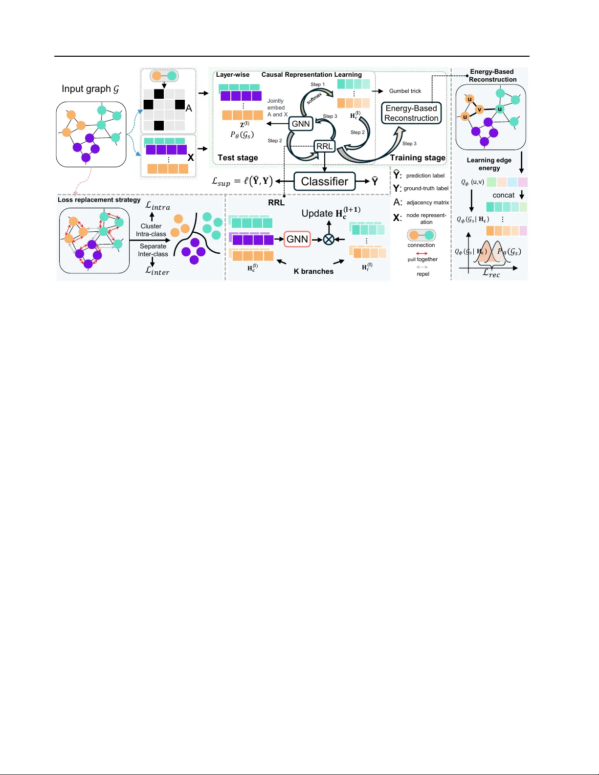
CGRL: Causal-Guided Repr esentation Learning f or Graph Out-of-Distrib ution Generalization Bowen Lu 1 Lianqiang Y ang 1 T eng Li 1 Abstract Graph Neural Networks (GNNs) have achieved impressiv e performance in graph-related tasks. Howe v er , they suf fer from poor generalization on out-of-distribution (OOD) data, as they tend to learn spurious correlations. Such correlations present a phenomenon that GNNs fail to sta- bly learn the mutual information between predic- tion representations and ground-truth labels under OOD settings. T o address these challenges, we formulate a causal graph starting from the essence of node classiﬁcation, adopt backdoor adjustment to block non-causal paths, and theoretically deri ve a lower bound for impro ving OOD generalization of GNNs. T o materialize these insights, we further propose a novel approach integrating causal repre- sentation learning and a loss replacement strategy . The former captures node-le vel causal in v ariance and reconstructs graph posterior distribution. The latter introduces asymptotic losses of the same order to replace the original losses. Extensiv e experiments demonstrate the superiority of our method in OOD generalization and effecti vely alleviating the phenomenon of unstable mutual information learning. 1. Introduction Graph-structured data ( Hu et al. , 2020 ) ubiquitously perme- ates real-world applications across diverse scenarios ( Ab- bahaddou et al. , 2024 ; Qiao et al. , 2025 ). In social net- works ( K ¨ uhne et al. , 2025 ), intricate inter-entity relation- ships are modeled using graphs, with nodes representing entities and edges encoding relationships. This has spurred a multitude of downstream tasks, such as community de- tection ( Fettal et al. , 2022 ), link prediction ( K ¨ uhne et al. , 2025 ), and node classiﬁcation ( Huang et al. , 2023 ; Jeong 1 School of Artiﬁcial Intelligence, Anhui Univ ersity , Hefei, China. Correspondence to: Lianqiang Y ang < yan- glq@ahu.edu.cn > . Preliminary work. 0 50 100 150 200 0 1 2 3 MI epoch (a) Cora dataset wit h feature shifts based on GCN (b) Cora dataset w ithout feature shifts based o n GCN 0 50 100 150 200 0 1 2 3 MI epoch F igure 1. Mutual information (MI) between GCN-based prediction representations and ground-truth labels on the Cora dataset with and without feature shifts. et al. , 2024 ). Against this backdrop, Graph Neural Networks (GNNs) ( Kipf & W elling , 2017 ; V eli ˇ ckovi ´ c et al. , 2018 ; W u et al. , 2019 ) have been proposed to learn prediction repre- sentations that integrate both topological structure and node feature information, thus enabling ef fective handling of di- verse graph-based do wnstream tasks. Despite the successes achiev ed by typical GNNs (e.g., GCN and GA T) in certain scenarios ( Xu et al. , 2024b ; Luo et al. , 2025 ), their per - formance often degrades under out-of-distrib ution (OOD) setting ( Hendrycks & Dietterich , 2019 ; Guo et al. , 2024 ). This shortcoming stems from the distrib ution shifts between training and test data ( W u et al. , 2022b ). T raditional GNNs rely on the independent and identically distributed (i.i.d.) assumption and tend to capture spurious correlations rather than causal relationships ( Chen et al. , 2022 ; 2023 ). T o substantiate this claim, we present empirical evidence. Fig. 1 illustrates the mutual information (MI) between GCN- based prediction representations and the ground-truth labels on the Cora dataset ( Sen et al. , 2008 ) with and without feature shifts. As a metric quantifying the statistical de- pendence between two random variables, MI between pre- diction representations and ground-truth labels exhibits an initial increase as the number of epochs grows, followed by pronounced ﬂuctuation on data with feature shifts. In contrast, for data without feature shifts, although the MI value undergoes de gradation, it maintains overall stability throughout the entire training process. These div ergent MI 1 CGRL: Causal-Guided Representation Lear ning for Graph Out-of-Distribution Generalization dynamics are attributed to the tendency of GNNs to over - rely on spurious correlations in in-distribution (ID) data. Such over -reliance not only leads to unstable prediction performance on OOD data b ut also induces a fundamental bottleneck for learning causal representations. ( Xu et al. , 2024a ; Zhao & Zhang , 2024 ; Zhang et al. , 2024 ). Note that this phenomenon is not exclusiv e to the Cora dataset ( He et al. , 2024 ). Therefore, incorporating causal representation learning is imperativ e to alleviate this issue. Recently , many studies ha ve focused on causal representa- tion learning to alleviate the impact of spurious correlations in GNNs on OOD data ( Ding et al. , 2025 ; An et al. , 2024 ; Y u et al. , 2025 ; Xia et al. , 2023 ). These methods learn en vironment-in variant representations across diverse set- tings ( Creager et al. , 2021 ; Liu et al. , 2023 ), enabling GNNs to adapt to distribution shifts and enhance their general- ization capability to unseen data. Lev eraging such causal learning paradigms, GNNs can be guided to focus on fea- tures causally related to the labels ( W ang et al. , 2024b ; Sui et al. , 2025 ) and attain stable MI between their prediction representations and the ground-truth labels. In this paper, we formulate a causal graph and leverage backdoor adjustment ( Pearl et al. , 2016 ) to block non-causal paths, and theoretically establish a lower bound for enhanc- ing the OOD generalization of GNNs. T o materialize these insights, we propose a novel Causal-Guided Representa- tion Learning (CGRL) framew ork. Our framew ork inte- grates causal representation learning and a loss replacement strategy . The former ef fectiv ely captures node-lev el causal in variance by dynamically adjusting the weights of node representations and realizes the reconstruction of the poste- rior distribution of graphs. The latter replaces the original losses with asymptotic losses of the same order . Extensiv e experiments demonstrate the superiority of our approach in OOD generalization and ef fectively alle viate the ﬂuctu- ation of mutual information. Our main contributions are summarized as follows: • W e ﬁrst uncov er the mutual information ﬂuctuation phenomenon of GNNs on OOD data, and attribute it to the tendency of GNNs to spurious correlations inherent in ID data. • W e deriv e a theoretical lo wer bound from a causal per- specti ve that for OOD generalization of GNNs. On this basis, we propose a novel CGRL framework, which effecti vely learns causal in variant representations and introduces asymptotic losses of the same order . • Extensi ve e xperiments on multiple benchmark datasets demonstrate that CGRL outperforms state-of-the-art methods and effecti vely alleviates the ﬂuctuation of mutual information in GNNs under OOD settings. 2. Background Notations. Let G = ( V , E ) denotes an input graph with node set V and edge set E . The set G = { G 1 , G 2 , ..., G S ′ } consists of S ′ subgraphs, where G s denotes the graph be- longing to the s -th ego-graph. Let N =  V  represent the number of nodes. A ∈ R N × N and the X ∈ R N × d de- note adjacency matrix and node representation, respecti vely , where d is representation dimension. For a node v ∈ V , N ( v ) = { u  v , u  ∈ E } is deﬁned as the set of its neighbors and deg ( v ) is its degree. For an edge  u, v  ∈ E , we hav e A [ u, v ] = 1 ; otherwise, A [ u, v ] = 0 . W e use H c and Y to represent the prediction representations and ground-truth labels, respectively . The goal of node classiﬁcation is to cluster intra-class nodes and separate inter -class nodes via H c . Thus, we denote the distrib ution of intra-class and inter- class nodes by H intra c and H inter c , respecti vely . S denotes the latent space of intra-class nodes, while D represents the latent space of inter-class nodes. Graph Neural Networks (GNNs). GNNs are primarily de- signed to handle graph-structured data with non-Euclidean structures ( Hamilton et al. , 2017 ; Xu et al. , 2019 ; Lee et al. , 2023 ). In the task of node classiﬁcation, they update the rep- resentation of each node by aggregating topological informa- tion and feature attrib utes among its neighbors, attempting to cluster intra-class nodes together and separate inter-class nodes, so as to achieve ef fective node discrimination. Its formulation is giv en as follows: H ( l + 1 ) v = U pdate { H ( l ) v , Ag g r eg ate { H ( l ) u  u ∈ N ( v ) }} , where Ag g r eg ate ( ⋅ ) denotes aggregation pattern between node v and its neighbors. U pdate ( ⋅ ) refers to the update function for node representations, which is typically a non- linear function (e.g., ReLU) employed to process the ag- gregated information. H ( l ) v and H ( l ) u represent the repre- sentations of node v and its neighbors at the ( l ) -th layer, respectiv ely . T ypical GNNs include Graph Con volutional Network (GCN) ( Kipf & W elling , 2017 ) and Graph Atten- tion Network (GA T) ( V eli ˇ ckovi ´ c et al. , 2018 ). The former aggregates node information in the spectral domain, while the latter incorporates attention mechanisms o ver nodes in the spatial domain. Howe ver , neither of them can stably learn the mutual information between prediction representa- tions and ground-truth labels. Energy-based Model (EBM). EBM ( Ranzato et al. , 2007 ; Grathwohl et al. , 2020 ; W u et al. , 2023 ) capture depen- dencies among v ariables by assigning scalar energies to them. In the OOD setting, the distribution discrepancy across graphs can be substantial. This calls for a highly ro- bust method that enables the model to learn causal features. Instead of lev eraging V ariational Autoencoders (V AEs) ( Kingma & W elling , 2014 ) and diffusion models ( Ho et al. , 2020 ), we use EBM which exhibit strong compatibility with 2 CGRL: Causal-Guided Representation Lear ning for Graph Out-of-Distribution Generalization graph data and are capable of capturing causal structural dependencies among nodes. It deﬁne an energy function E θ ( X 1 , X 2 ) between two variables X 1 and X 2 , where θ denotes the learnable parameters. Then, its probability dis- tribution is represented as follo ws: P θ ( X 1 , X 2 ) = e − E θ ( X 1 ,X 2 ) ∑ x e − E θ ( X 1 ,X 2 ) The energy score E θ ( X 1 , X 2 ) can model the dependencies between X 1 and X 2 , which can serve as a key method for learning stable mutual information between prediction representations and ground-truth labels. Howe ver , current research on ener gy-based modeling and its applications in causal representation learning remain underexplored, and the potential of energy-based models in the stable modeling of interdependent data has not yet been fully exploited. Y E 𝒢 A X 𝐇 𝐜 𝐇 𝐜 𝐢𝐧 𝐭 𝐞 𝐫 𝐇 𝐜 𝐢𝐧𝐭𝐫 𝐚 𝒢 : Inp ut graph E : Noi s e Y : G r o u n d - truth l a b e l A : A dj ac en c y m atri x X : Nod e repres en tat i on 𝐇 𝐜 : P r ed i c ti on r ep r es en tat i on 𝐇 𝐜 𝐢𝐧 𝐭𝐫 𝐚 : Di s tr i bu ti on of i ntra - c l as s no de 𝐇 𝐜 𝐢𝐧 𝐭𝐞 𝐫 : Di s tr i bu ti on of i nte r - c l as s no de F igure 2. Causal graph. 3. Methodology In this section, we ﬁrst analyze the reason why GNNs fail to stably learn the mutual information between prediction rep- resentations and ground-truth labels and GNNs struggle to generalize to unseen data in Section 3.1 . Then, Based on the this analysis, we deri ve a theoretical lo wer bound to guide model optimization. Finally , leveraging these theoretical foundations, we introduce a novel Causal-Guided Repre- sentation Learning (CGRL) frame work tailored to address OOD problems in Fig. 3 . 3.1. A Causal Perspecti ve for Graph OOD Generalization T o clarify the phenomenon in Fig. 1 and the reasons for the poor generalization of GNNs, we conduct an analysis from a causal perspectiv e ( Pearl , 2009 ), as illustrated in Fig. 2 . Speciﬁcally , we formulate a causal graph grounded in the Structural Causal Model (SCM) ( Pearl et al. , 2016 ), where directed arrows denote causal relationships between vari- ables. This causal graph comprises eight elements: noise E , input graph G , adjacency matrix A , node representation X , prediction representation H c , intra-class distrib ution H intra c and inter-class distrib ution H inter c . Detailed descriptions of the causal relationships are provided as follo ws: • Y ← E → G : Noise E from environment induces distribution shifts in both the input graph G and the distribution of ground-truth label Y . • A ← G → X : The input graph G is jointly constituted by the adjacency matrix A (topological structure) and node representation X (node feature information). • H intra c ← H c → H inter c : T o achiev e the goal of node classiﬁcation, GNNs aim to cluster intra-class nodes and separate inter-class nodes as much as possible. Thus, the prediction representation H c is jointly com- posed of intra-class distribution H intra c and inter-class distribution H inter c . • H intra c → Y : The distrib ution H intra c can determine the ground-truth label Y . This is because the goal of node classiﬁcation can only be achiev ed by clustering intra-class nodes in their respectiv e latent spaces. T raditional statistical methods ev aluate the inﬂuence of H c on Y by directly calculating the conditional probability P ( Y  H c ) ( Sui et al. , 2022 ). Howe ver , the causal graph rev eals three backdoor paths: H inter c ← H c → H intra c → Y , H c ← A ← G ← E → Y , and H c ← X ← G ← E → Y . SCM theoretically demonstrates that the estimation of P ( Y  H c ) is affected by these non-causal paths ( Pearl , 2014 ), which stems from two key variables. First, due to the structure H inter c ← H c → H intra c , non-causal ﬂow arises between H inter c and H intra c . Intra-class nodes tend to separate rather than cluster , blurring the discriminability of node representations and interfered with stability of the mutual information between prediction representations and ground-truth labels. Second, the confounding effect of E introduce noise into H c , which interferes with prediction performance and undermines the generalization capability of GNNs ( Sui et al. , 2024 ). These two variables lead GNNs to learn spurious and unstable prediction patterns, resulting in the mutual information ﬂuctuation between H c and Y . T o accurately ev aluate the causal effect between H c and Y , we resort to do - c alculus from SCM and perform backdoor adjustment to intervene on H c , i.e., P ( Y  do ( H c )) . Ide- ally , such an ev aluation could be achieved via Randomized Controlled T rial (RCT). Y et the existing of the unobserv ed variable E in the causal graph renders this approach infeasi- ble. Instead, the following theorem demonstrates that direct calculation of P ( Y  do ( H c )) can be achie ved without E . Theorem 3.1. Given a causal graph in F ig. 3 , we can obtain a equation that estimate causal relationships fr om H c to Y : P θ ( Y  do ( H c )) = E P θ ( G s ) P θ ( Y  H c , G s ) (1) wher e θ r epresents par ameter of the model. 3 CGRL: Causal-Guided Representation Lear ning for Graph Out-of-Distribution Generalization In p u t g rap h 𝒢 A X … C lass if ier ෡ Y C lus t e r I n t r a - c las s S e p a r a t e I n t e r - c la s s 𝐇 𝐜 𝐥 p r e d iction lab e l Upd a te 𝐇 𝐜 𝐥 + 𝟏 u u v u … 𝑄 𝜙 ( 𝒢 𝑠 | 𝐇 𝐜 ) E ner gy - B a s e d R e c onst ruc t i on ෡ Y : co n n e ctio n p u l l to g e th e r repe l A: a d jace n cy m a tr ix X : n o d e r e p r e se n t - a tio n … GNN Lea rni ng e dge e ner gy … T es t stag e G NN RRL E ne r g y - B as e d Rec on s tr uc ti on T r ainin g stag e 𝐙 𝐥 Jo in t ly e m b e d A a n d X RRL Y : ground - tr u t h lab e l Lay e r - w i s e S te p 1 S te p 3 S te p 2 S te p 2 S te p 3 c o n c a t 𝑄 𝜙 ( u , v ) 𝑃 𝜃 𝒢 𝑠 𝐇 r 𝐥 𝐇 r 𝐥 𝑃 𝜃 𝒢 𝑠 𝑄 𝜙 ( 𝒢 𝑠 | 𝐇 𝐜 ) K bra nc he s Gu m b e l tr ick … C a usa l R e pre s e nt a t i on Lea rni ng Loss re pl a c e m e nt s t ra t e gy ℒ 𝑠 𝑢 𝑝 = 𝓁 ෠ 𝐘 , 𝐘 ℒ 𝑟𝑒𝑐 ℒ 𝑖 𝑛 𝑡𝑟 𝑎 ℒ 𝑖 𝑛 𝑡𝑒 𝑟 F igure 3. The CGRL framew ork consists of two parts: causal representation learning and loss replacement strategy . The former includes re-weight representation learning (RRL) and energy-based reconstruction. They captures node-level in variance and performs graph reconstruction to yield the reconstruction loss L rec . Speciﬁcally , the adjacency matrix A and node representation X are fed into a GNN encoder to learning representation Z (i.e., P θ ( G s ) ). In the testing phase, Z is sequentially processed by the softmax and the RRL module, producing H r and the prediction representation H c , respectiv ely . In contrast, the training phase in volves a sequence of operations on Z : Gumbel trick, RRL, and energy-based reconstruction. The ﬁnal H c is fed into a classiﬁer for prediction, yielding the supervised loss L sup . T o achieve the optimization objecti ves of clustering intra-class and separating inter-class, the latter introduces asymptotic losses of the same order to replace the original losses, which giv es rise to the intra-class loss L intra and inter-class loss L inter . The proof is provided in Appendix A.1 . Eqn. 1 re veals our optimization objectiv e in terms of log-likelihood: L ( Θ ) = arg max Θ log E P θ ( G s ) P θ ( Y  H c , G s ) (2) where Θ = { θ 1 , θ 2 , ..., θ n } is the set of all the parameters in the model. While Eqn 1 establishes the optimization objectiv e of the model, it only mitigates the confounding effect of E . Thus, additional constraints in volving H inter c need to be introduced. 3.2. Theoretical Lo wer Bound While Eqn. 1 establishes a formulation for calculating P ( Y  do ( H c )) , directly optimizing it remains non-trivial. T o facilitate the optimization process and constrain H inter c , we deriv e a theoretical lower bound as follo ws: Theorem 3.2. Suppose that Q ϕ ( G s  H c ) , Q ϕ ( H intra c  H c ) and Q ϕ ( H inter c  H c ) serve as posterior appr oximations of P θ ( G s ) , P θ ( H intra c  H c ) and P θ ( H inter c  H c ) , r espectively . Based on Eqn 2 , the lower bound is formulated as: L ( Θ; ϕ ) ≥ E Q ϕ ( G s  H c ) E Q ϕ ( H intra c  H c ) log P θ ( Y  H c , H intra c , G ) − KL ( Q ϕ ( G s  H c ) P θ ( G s )) − KL ( Q ϕ ( H intra c  H c ) P θ ( H intra c  H c )) − KL ( Q ϕ ( H inter c  H c ) P θ ( H inter c  H c )) , (3) wher e ϕ is parameter of posterior distribution and KL ( ⋅ ) denotes the K ullback-Leibler diver gence. The proof is provided in Appendix A.2 . By optimizing the lower bound presented in Theorem 3.2 , we enable the model to perform iterati ve backpropagation for parameter Θ and ϕ . Next, we elaborate on the detailed learning strategy for this optimization objectiv e, thereby facilitating the ev aluation of the causal effect from H c to Y . 3.3. Causal Representation Lear ning T o achiev e that optimization objectiv e, we ﬁrst process G s by embedding nodes into the latent space. Since the input graph G s of the s -th ego-graph is jointly constituted by the adjacency matrix A and node representation X , we feed both components into a GNN encoder , which allows us to simultaneously obtain hybrid embedded representation Z (i.e., P( G s )). Next, we introduce causal representation learning module. 3 . 3 . 1 . R E - W E I G H T R E P R E S E N TA T IO N L E A R N I N G T o obtain the prediction representation H c , we initialize H ( 0 ) c with the output Z ( 1 ) of the ﬁrst GNN encoding pass, then feed the learned H c as input to the Z of the subsequent layer . Inspired by GLIND ( W u et al. , 2024b ), instead of 4 CGRL: Causal-Guided Representation Lear ning for Graph Out-of-Distribution Generalization directly learning H c from the GNNs, we assign dif ferent weights to the representation of each node. This enables the model to adapti vely adjust node representations via re- weighting. Prior to the generation of H c , we compute the weight matrix H r from Z using the softmax function during the test phase. H ( l + 1 ) r = exp ( Z ( l ) v ) ∑ v ∈ V exp ( Z ( l ) v ) , After that, we design distinct encoders tailored to dif ferent types of GNNs. CGRL-GCN. Inspired by the K -head attention mechanism and canonical GCN architectures, we design K branches to perform node representations learning. For the GCN-based encoder ( Kipf & W elling , 2017 ), we formulate the following expression: H ( l + 1 ) c = H ( l ) c + σ ( K  k = 1  u ∈ N ( v ) 1 C uv H ( l ) r H ( l ) c W ( l,k ) c ) , where C uv =  deg ( v )  deg ( u ) , W ( l,k ) c ∈ R d × d is learn- able weight at the l -th layer and k -th branch. CGRL-GA T . Owing to the inherent compatibility between attention-based networks and the K branches, we can simi- larly apply the re-weighted matrix H r to the Graph Atten- tion Network (GA T) ( V eli ˇ ckovi ´ c et al. , 2018 ). H ( l + 1 ) c = H ( l ) c + σ ( K  k = 1  u ∈ N ( v ) H ( l ) r α ( k,uv ) H ( l ) c W ( l,k ) c ) , α ( k,uv ) = exp ( Leak y ReLu ( e ( k,uv ) )) ∑ u ′ ∈ N ( v ) exp ( Leak y ReLu ( e ( k,u ′ v ) )) , e ( k,uv ) = a ( l,k ) T [ W ( l,k ) α H ( l ) ( c,v )  W ( l,k ) α H ( l ) c,u ] T , where W ( l,k ) α ∈ R d × d and a ( l,k ) ∈ R 2 d denote learnable weight matrices at the l -th layer and k -th branch. Symbol [ ⋅  ⋅ ] represents concatenation operation. Through this representation reweighting approach, the model can assign higher weights to nodes with greater importance, thereby capturing the causal in variance within nodes. Based on different GNNs, we obtain the re-weighted pre- diction representation H c via the aforementioned design, which serv es as a prerequisite for the subsequent reconstruc- tion of graph G s . 3 . 3 . 2 . E N E R G Y - BA S E D R E C O N S T R U C T I O N Building on the distribution P θ ( G s ) , our goal is to deri ve the posterior distribution Q ϕ ( G s  H c ) to optimize the second loss term in Eqn 3 . During the training phase, we recon- struct the attrib ute features of G s through an ener gy-based model, lev eraging the prediction representation H c . This reconstruction strategy models the intrinsic structure of the graph and the dependencies among nodes, enabling GNNs to yield stable predictions and thus enhancing their general- ization performance. For interconnected nodes v and u (i.e., A [ u, v ] =1), we deﬁne energy of the edge  u, v  as E ( u, v ) . Q ϕ ( u, v ) = exp ( − E ( u, v )) ∑ u ∈ N ( v ) exp ( − E ( u, v )) , E ( u, v ) = − H ( c,v ) W uv H T ( c,u ) , where W uv ∈ R d × d denotes a learnable weight matrix. The energy function E ( u, v ) quantiﬁes the energy-based similarity for each edge  u, v  . The lo wer the energy of interconnected nodes u and v , the higher the probability of an edge existing between them in the input graph G s . Instead of applying the softmax function, we leverage the Gumbel trick ( Jang et al. , 2017 ) on the representation Z to implement sampling over the distrib ution P ( G s ) during the training phase. Appendix F elaborates on the rationale for its adoption. Q ϕ ( G s ) = exp (( Z ( l ) v + g k )/ τ ) ∑ k ′ exp (( Z ( l ) v + g k ′ )/ τ ) , where g k = − log ( − log ( u i )) , u i ∼ U ( 0 , 1 ) and τ controls the degree of discreteness of the distrib ution. Then, we ob- tain the reconstructed posterior distrib ution as Q ϕ ( G  H c ) = [ Q ϕ ( G s ) Q ϕ ( u, v )] . Although energy-based model suf- fers from the challenge of training difﬁculty , this recon- struction strategy enables CGRL to achiev e full gradient descent. In the end, we are able to deriv e the second loss term − KL ( Q ϕ ( G s  H c ) P θ ( G s )) in Eqn 3 . By regulariz- ing the estimation of graph G , this term prev ents the CGRL from overﬁtting to the noise embedded in H c and av oids generating an unreasonable topological estimation of G s , which pro vides a robust topological foundation for the learn- ing of representation Z and the effecti ve utilization of the adjacency matrix A . L rec ( Θ; ϕ ) = min Θ  G s Q ϕ ( G s  H c ) log Q ϕ ( G s  H c ) P θ ( G s ) (4) 3.4. Optimization Intra-class and Inter -class Loss. The last two loss terms in Eqn 3 are − KL ( Q ϕ ( H intra c  H c ) P θ ( H intra c  H c )) and − KL ( Q ϕ ( H inter c  H c ) P θ ( H intra c  H c )) . For the former term, given that intra-class nodes share similar connectiv- ity patterns in the ego-graph G s , this term regularizes the causal path H c → H intra c → Y and mitigates the con- founding effects of all the backdoor paths. It achieves the goal of clustering intra-class nodes by aligning the distribu- tion Q ϕ ( H intra c  H c ) with the distribution P θ ( H intra c  H c ) . 5 CGRL: Causal-Guided Representation Lear ning for Graph Out-of-Distribution Generalization When the distribution of H intra c for intra-class nodes re- mains maximally inv ariant under the constraints imposed by H c , this enables stable prediction of the ground-truth label Y and blocks the effect of the backdoor paths induced by the H inter c and E . For the latter term, it can strengthen the separation property of inter-class nodes in the latent space since the discreteness of H inter c undermine the con- centration of inter-class nodes. In turn, it minimizes the ov erlap of node representations across different classes, thereby enhancing the model’ s capacity to discriminate between inter-class nodes. Howe ver , the distributions of P θ ( H intra c  H c ) and P θ ( H inter c  H c ) are unknown and in- tractable to obtain, which poses challenges for the model to learn Q ϕ ( H intra c  H c ) and Q ϕ ( H inter c  H c ) . T o implement these two optimization objecti ves (i.e., intra-class aggre ga- tion and inter-class separation), we propose the following lemma. Lemma 3.3. The ultimate goal of optimizing KL ( Q ϕ ( H intra c  H c ) P θ ( H intra c  H c )) and KL ( Q ϕ ( H inter c  H c ) P θ ( H inter c  H c )) is Q ϕ = P θ . Then, Q ϕ ( H intra c  H c ) w − → P θ ( H intra c  H c ) , Q ϕ ( H inter c  H c ) w − → P θ ( H inter c  H c ) , wher e w − → denotes weak con ver gence. Based on Lemma 3.3 and Assumption B.1 presented in Appendix B , the follo wing theorem introduces alternative forms for the two loss terms. Theorem 3.4. Under the pr emise of the ideal GNNs with the number of iterations T → ∞ and Assumption B.1 holds, the intra-class/inter-class losses and their corr esponding KL diver gence losses ar e equal in the limit and of the same or der . lim T → ∞ L intra KL ( Q ϕ ( H intra c  H c )) P θ ( H intra c  H c )) = c 1 ≠ 0 , lim T → ∞ L inter KL ( Q ϕ ( H inter c  H c )) P θ ( H inter c  H c )) = c 2 ≠ 0 , (5) wher e T is the number of epochs. While certain distributions remain intractable, per Eqn 5 , when the optimal model performs T epochs ( T → ∞ ) , L intra and L inter exhibit asymptotic equi valence in order to their respectiv e counterpart losses. By virtue of this order - based approximation, we can substitute the original losses to attain the goal of the identical node classiﬁcation. Prediction Loss. For the ﬁrst term in Eqn 3 is E Q ϕ ( G s  H c ) E Q ϕ ( H intra c  H c ) log P θ ( Y  H c , H intra c , G s ) , we hav e already obtained Q ϕ ( G s  H c ) via the aforementioned graph reconstruction. Moreov er, as pro ven in Theorem 4.4, we replaces the original losses with asymptotic losses of the same order . W e take H c , obtained after clustering intra-class nodes and separating inter-class nodes, as the prediction la- bel ˆ Y . This loss term is thus deﬁned as the cross-entropy loss L sup between ˆ Y and the ground-truth label Y . Finally , we have obtained all the loss terms of CGRL. By combining the four aforementioned loss terms, the ov erall optimization formulation is giv en as follows: L ( Θ; ϕ ) = min Θ L sup + L rec + λ 1 L intra + λ 2 L inter , where λ 1 and λ 2 are the loss weights. 4. Experiments In this section, to v erify the generalization performance of our proposed CGRL framework, we conduct experiments on 8 open-source datasets with public split and address the following questions. RQ1: Ho w does model performs compared to baselines? RQ2: Do proposed model learns steadily mutual informa- tion between prediction representations and ground-truth labels? RQ3: How does each module contributes to the perfor- mance? T o induce distribution shifts, we adopt two distinct public data splitting strategies, respectively proposed by CaNet ( W u et al. , 2024a ) and GOOD ( Gui et al. , 2022 ). These implementation details of this experiment are in Appendix C and sensitivity analysis are detailed in Appendix F . 4.1. Overall P erformance Comparison (RQ1) 4 . 1 . 1 . G E N E R A L I Z A T I O N O N F E A T U R E A N D S PA T I O T E M P O R A L S H I F T S W e present comparisons in T able 1 between CGRL and base- lines with GCN- and GA T -based models on ﬁv e datasets with feature and spatiotemporal shifts. W e draw the follo w- ing observations: (1) CGRL achiev es superior generaliza- tion performance over all baselines on the Cora, Citeseer , and Pubmed datasets with feature shifts, demonstrating its strong generalization capability . Particularly , our model de- liv ers notably substantial performance gains on the Pubmed dataset, outperforming the second-best model by 6.93% and 4.73% on GCN- and GA T -based models, respectiv ely . (2) Our model surpasses CaNet in generalization performance on the Arxiv dataset with temporal shifts and the T witch dataset with spatial shifts. This indicates that CGRL can learn highly discriminati ve prediction representations e ven in the presence of sev ere distribution shifts. (3) Our method outperforms the con ventional Empirical Risk Minimization (ERM) algorithm by a signiﬁcant mar gin. This is because ERM tends to capture spurious c orrelations, which limits the 6 CGRL: Causal-Guided Representation Lear ning for Graph Out-of-Distribution Generalization T able 1. T est (mean±standard de viation) Accuracy (%) and R OC-A UC (%) on OOD data of Arxi v and T witch datasets, respecti vely . OOM denotes out-of-memory . Bold numbers indicate the best result, and the underlined numbers indicate the second-best result. Backbone Method Cora Citeseer Pubmed Arxiv T witch 2014-2015 2016-2017 2018-2020 ES FR EN GCN ERM 74.30 ±2.66 74.93 ±2.39 81.36 ±1.78 56.33 ±0.17 53.53 ±0.44 45.83 ±0.47 66.07 ±0.14 52.62 ±0.01 63.15 ±0.08 IRM 74.19 ±2.60 75.34 ±1.61 81.14 ±1.72 55.92 ±0.24 53.25 ±0.49 45.66 ±0.83 66.95 ±0.27 52.53 ±0.02 62.91 ±0.08 Coral 74.26 ±2.28 74.97 ±2.53 81.56 ±2.35 56.42 ±0.26 53.53 ±0.54 45.92 ±0.52 66.15 ±0.14 52.67 ±0.02 63.18 ±0.03 D ANN 73.09 ±3.25 74.74 ±2.78 80.77 ±1.43 56.35 ±0.11 53.81 ±0.33 45.89 ±0.37 66.15 ±0.13 52.66 ±0.02 63.20 ±0.06 GroupDR O 74.25 ±2.61 75.02 ±2.05 81.07 ±1.89 56.52 ±0.27 53.40 ±0.29 45.76 ±0.59 66.82 ±0.26 52.69 ±0.02 62.95 ±0.11 Mixup 92.77 ±1.27 77.28 ±5.28 79.76 ±4.44 56.67 ±0.46 54.02 ±0.51 46.09 ±0.58 65.76 ±0.30 52.78 ±0.04 63.15 ±0.08 SRGNN 81.91 ±2.64 76.10 ±4.04 84.75 ±2.38 56.79 ±1.35 54.33 ±1.78 46.24 ±1.90 65.83 ±0.45 52.47 ±0.06 62.74 ±0.23 EERM 83.00 ±0.77 74.76 ±1.15 OOM OOM OOM OOM 67.50 ±0.74 51.88 ±0.07 62.56 ±0.02 CaNet 96.12 ±1.04 94.57 ±1.92 88.82 ±2.30 59.01 ±0.30 56.88 ±0.70 56.27 ±1.21 67.47 ±0.32 53.59 ±0.19 64.24 ±0.18 CIA-LRA 97.43 ±0.28 94.22 ±0.31 89.97 ±0.17 OOM OOM OOM 67.19 ±0.43 53.08 ±0.92 64.03 ±0.32 CGRL (ours) 99.14 ±0.16 97.96 ±0.23 96.90 ±0.44 60.28 ±0.37 60.07 ±0.52 58.14 ±0.93 68.02 ±0.29 54.98 ±0.23 64.89 ±0.12 GA T ERM 91.10 ±2.26 82.60 ±0.51 84.80 ±1.47 57.15 ±0.25 55.07 ±0.58 46.22 ±0.82 65.67 ±0.02 52.00 ±0.10 61.85 ±0.05 IRM 91.63 ±1.27 82.73 ±0.37 84.95 ±1.06 56.55 ±0.18 54.53 ±0.32 46.01 ±0.33 67.27 ±0.19 52.85 ±0.15 62.40 ±0.24 Coral 91.82 ±1.30 82.44 ±0.58 85.07 ±0.95 57.40 ±0.51 55.14 ±0.71 46.71 ±0.61 67.12 ±0.03 52.61 ±0.01 63.41 ±0.01 D ANN 92.40 ±2.05 82.49 ±0.67 83.94 ±0.84 57.23 ±0.18 55.13 ±0.46 46.61 ±0.57 66.59 ±0.38 52.88 ±0.12 62.47 ±0.32 GroupDR O 90.54 ±0.94 82.64 ±0.61 85.17 ±0.86 56.69 ±0.27 54.51 ±0.49 46.00 ±0.59 67.41 ±0.04 52.99 ±0.08 62.29 ±0.03 Mixup 92.94 ±1.21 82.77 ±0.30 81.58 ±0.65 57.17 ±0.33 55.33 ±0.37 47.17 ±0.84 65.58 ±0.13 52.04 ±0.04 61.75 ±0.13 SRGNN 91.77 ±2.43 82.72 ±0.35 83.40 ±0.67 56.69 ±0.38 55.01 ±0.55 46.88 ±0.58 66.17 ±0.03 52.84 ±0.04 62.07 ±0.04 EERM 91.80 ±0.73 74.07 ±0.75 OOM OOM OOM OOM 66.80 ±0.46 52.39 ±0.20 62.07 ±0.68 CaNet 97.30 ±0.25 95.33 ±0.33 89.89 ±1.92 60.44 ±0.27 58.54 ±0.72 59.61 ±0.28 68.08 ±0.19 53.49 ±0.14 63.76 ±0.17 CIA-LRA 97.89 ±0.34 95.47 ±0.09 92.12 ±0.22 OOM OOM OOM 67.76 ±0.29 53.26 ±0.37 63.68 ±0.25 CGRL (ours) 98.56 ±0.17 97.74 ±0.16 96.83 ±0.21 61.57 ±0.32 60.40 ±0.48 60.78 ±0.41 68.42 ±0.25 54.51 ±0.17 64.23 ±0.21 upper bound of learning for GNNs. This v alidates that the optimization objecti ves introduced in Section 3.4 ef fectiv ely mitigate the confounding ef fects in non-causal paths. 4 . 1 . 2 . G E N E R A L I Z AT I O N O N C OV A R I A T E A N D C O N C E P T S H I F T S In this section, we further conduct comparative e xperiments in T able 2 between CGRL and baselines with GCN- and GA T -based models on three datasets with cov ariate and concept shifts. The key observ ations are summarized as fol- lows: (1) CGRL attains the optimal performance on datasets with cov ariate shifts. This veriﬁes that CGRL can alle viate the performance degradation induced by distrib ution shifts, ev en when discrepancies exist between the training and test distributions. (2) CGRL yields consistent performance im- prov ements on most datasets with concept shifts, with the exception of GOODCB AS with a GCN-based model. This is attributed to the fact that our model captures in variance in prediction representations by learning causal represen- tations. Even on GOODCBAS with a GCN-based model, our model still ranks second in performance. (3) CGRL can achiev e good adaptation across different domains under the same shifts or under different shifts, which demonstrates that it possesses high robustness and can still achiev e fav or- able accuracy e ven when tackling cross-domain tasks. 4.2. Alleviate Fluctuation of Mutual Inf ormation (RQ2) Fig. 4 depicts the mutual information (MI) between all pre- diction representations and ground-truth labels on the Cora and Citeseer datasets, as deri ved from CGRL. Unlike base- lines with GCN- and GA T -based models, although the MI can ﬂuctuate during the initial training iterations, it exhibits an ov erall upward trend. As the number of epochs grows, the MI values sho w minimal ﬂuctuation and gradually stabilize, demonstrating a clear tendency toward con vergence. This in- dicates that CGRL can steadily learn causal representations instead of spurious correlations and mitigate confounding effects from non-causal paths. Furthermore, a comparison between Fig. 1 and Fig. 4 (a) reveals that CGRL achie ves substantially higher MI values. This is because spurious cor - relations impose an inherent learning bottleneck on GNNs, which validates the ef fectiv eness of our causal representa- tion learning paradigm. By capturing in variance in node representations, our model achiev es superior generalization performance and pushes the performance upper bound of GNNs. More detailed experiments related to it are presented in Appendix D . 4.3. Ablation Studies (RQ3) In this section, to v alidate the effecti veness of each loss com- ponent in CGRL, we design four variants of the model: w/o L sup (ablation of the prediction loss), w/o L rec (ablation of the reconstruction loss), w/o L intra (ablation of the intra- class loss), and w/o L inter (ablation of the inter-class loss), where “w/o” denotes the model without the corresponding loss. The experimental results on the GCN-based model are summarized in T able 3 . First, we observe that the generaliza- tion performance of the model de grades across all datasets when any single loss component is ablated, demonstrating 7 CGRL: Causal-Guided Representation Lear ning for Graph Out-of-Distribution Generalization T able 2. T est (mean±standard deviation) Accuracy (%) on OOD data of GOODCora, GOODCB AS and GOOODW ebKB datasets under the different shifts, respectiv ely . OOM denotes out-of-memory . Bold numbers indicate the best result, and the underlined numbers indicate the second-best result. Backbone Method Covariate Concept GOODCora GOODCBAS GOOD W ebKB GOODCora GOODCB AS GOOD W ebKB degree word color university degree word color univ ersity GCN ERM 55.78 ±0.52 64.76 ±0.30 78.57 ±2.02 16.14 ±1.35 60.24 ±0.40 64.32 ±0.15 82.14 ±1.17 27.52 ±0.75 IRM 55.77 ±0.66 64.81 ±0.33 78.57 ±1.17 13.75 ±4.91 61.23 ±0.08 64.42 ±0.18 81.67 ±0.89 27.52 ±0.75 Coral 56.03 ±0.37 64.75 ±0.26 78.09 ±0.67 11.90 ±1.72 60.41 ±0.27 64.34 ±0.17 82.86 ±0.58 26.61 ±0.75 D ANN 56.10 ±0.59 64.77 ±0.42 77.57 ±2.86 15.08 ±0.37 60.78 ±0.38 64.51 ±0.19 82.50 ±0.72 26.91 ±0.36 GroupDR O 55.64 ±0.50 64.62 ±0.30 79.52 ±0.67 14.29 ±2.59 60.59 ±0.36 64.34 ±0.25 82.38 ±0.67 28.44 ±0.01 Mixup 57.89 ±0.27 65.07 ±0.22 70.00 ±5.34 16.67 ±1.12 63.65 ±0.37 64.45 ±0.12 65.48 ±0.67 30.28 ±1.50 SRGNN 57.13 ±0.25 64.50 ±0.35 73.81 ±4.71 16.40 ±1.63 61.21 ±0.29 64.53 ±0.27 80.95 ±0.67 27.52 ±0.75 EERM 56.88 ±0.32 61.98 ±0.1 40.48 ±9.87 16.21 ±5.67 58.38 ±0.04 63.09 ±0.36 61.43 ±1.17 28.04 ±11.67 CaNet 57.35 ±0.04 64.66 ±0.36 80.95 ±0.67 15.61 ±5.51 60.34 ±0.20 64.65 ±0.39 83.24 ±3.32 26.30 ±0.43 CIA-LAR 58.40 ±0.59 65.95 ±0.04 82.86 ±1.17 19.84 ±2.83 63.71 ±0.32 65.07 ±0.21 94.53 ±0.33 36.70 ±0.75 CGRL (ours) 59.68 ±0.47 69.01 ±0.21 83.14 ±1.51 23.02 ±2.37 65.51 ±0.23 68.15 ±0.28 85.29 ±1.13 39.27 ±1.02 GA T ERM 55.30 ±0.34 63.75 ±0.39 65.24 ±2.69 31.48 ±6.12 61.36 ±0.38 64.38 ±0.13 74.52 ±1.87 25.69 ±1.98 IRM 55.07 ±0.30 63.75 ±0.26 65.24 ±1.78 30.69 ±8.63 61.42 ±0.34 64.31 ±0.39 73.33 ±0.89 25.69 ±1.98 Coral 55.35 ±0.40 63.96 ±0.07 64.76 ±2.43 33.86 ±6.93 61.62 ±0.26 64.26 ±0.28 75.95 ±3.21 30.27 ±3.26 D ANN 55.31 ±0.57 64.21 ±0.12 65.44 ±3.18 32.43 ±2.09 61.59 ±0.31 64.41 ±±0.24 74.04 ±2.38 26.87 ±2.07 GroupDR O 55.03 ±0.45 63.82 ±0.06 67.62 ±2.43 31.75 ±2.82 61.31 ±0.20 64.07 ±0.25 73.81 ±1.78 26.91 ±2.16 Mixup 56.77 ±0.36 65.70 ±0.28 63.33 ±8.60 20.37 ±11.38 63.97 ±0.18 65.42 ±0.32 73.33 ±1.47 38.53 ±0.75 SRGNN 55.87 ±0.32 64.50 ±0.35 68.09 ±0.67 28.84 ±1.35 61.21 ±0.29 64.10 ±±0.28 72.38 ±1.22 23.55 ±1.56 EERM 46.63 ±1.75 62.57 ±0.50 60.47 ±4.10 33.33 ±14.60 48.05 ±2.03 53.02 ±1.23 60.95 ±3.56 25.38 ±4.26 CaNet 55.35 ±0.14 62.76 ±0.25 68.09 ±1.78 23.87 ±15.16 60.97 ±0.07 63.73 ±0.44 75.95 ±3.41 24.77 ±3.97 CIA-LRA 57.95 ±0.13 68.59 ±0.26 75.24 ±1.78 38.62 ±3.57 67.08 ±0.26 68.05 ±0.14 78.34 ±3.51 31.80 ±1.88 CGRL (ours) 60.05 ±0.14 69.37 ±0.17 77.56 ±2.59 42.33 ±3.28 68.67 ±0.43 70.84 ±0.45 83.57 ±1.01 39.45 ±1.54 0 50 100 150 200 0.0 0.7 1.4 2.1 2.8 MI epoch (a) Cora(GCN) 0 50 100 150 200 0.0 0.7 1.4 2.1 2.8 MI epoch (b) Cora(GAT) 0 50 100 150 200 0.0 0.7 1.4 2.1 2.8 MI epoch (c) Citeseer(GCN) 0 50 100 150 200 0.0 0.7 1.4 2.1 2.8 MI epoch (d) Citeseer(GAT) F igure 4. Mutual information on Cora and Citeseer datasets with feature shifts between prediction representations and ground-truth labels based on CGRL. As the number of epochs grows, the value of mutual information exhibits a tendenc y of conv ergence. that each loss term is indispensable to the model. Note that the model with L sup ablated exhibits the most pronounced performance degradation and e ven achiev es lower accuracy than the baselines. As it refers to the cross-entropy loss between prediction representations and ground-truth labels, this result highlights the critical importance of it for node classiﬁcation tasks. Second, the variants w/o L rec , w/o L intra , and w/o L inter also suf fer from a certain degree of performance degradation. This is mainly attributed to the fact that these loss components regularize the energy-based learning of graph reconstruction, facilitate intra-class node T able 3. The results of the ablation study based on GCN. Methods Cora Citeseer Pubmed GOODCora w/o L sup 70.34 ±1.17 69.89 ±2.31 78.52 ±2.17 53.28 ±0.18 w/o L rec 91.78 ±0.32 87.12 ±0.19 85.73±0.41 55.41 ±0.52 w/o L intra 96.64 ±0.23 94.14 ±0.21 90.81 ±0.59 56.58 ±0.36 w/o L inter 97.57 ±0.21 95.40 ±0.18 92.47 ±0.31 57.83 ±0.24 CGRL (ours ) 99.14 ±0.16 97.96 ±0.23 96.90 ±0.44 59.68 ±0.47 clustering, and enforce inter-class node separation. These components are crucial for reﬁning causal representations in the latent space, thereby enhancing the model’ s general- ization performance across div erse data distributions. 5. Conclusion In conclusion, this paper addresses the mutual information ﬂuctuation issue of GNNs on OOD data from a causal per- spectiv e. W e formulate a causal graph, deriv e a theoretical lower bound for enhancing OOD generalization of GNNs, and propose a novel CGRL framework with causal repre- sentation learning and a loss replacement strategy . The for- mer captures node-le vel causal in v ariance and reconstructs graph posterior distribution. The latter introduces asymp- totic losses of the same order to replace the original losses. Extensiv e experiments demonstrate the superiority of our method in OOD generalization and ef fectiv ely alleviates the ﬂuctuation of mutual information. The potential limitation of this frame work is that it may hav e high time complexity on large-scale graphs. 8 CGRL: Causal-Guided Representation Lear ning for Graph Out-of-Distribution Generalization Impact Statement This work aims to enhance the generalization of models in the ﬁeld of Graph Machine Learning on data outside the training distribution from a causal perspecti ve and by stabi- lizing mutual information learning. As graph data underpins modern artiﬁcial intelligence across healthcare, ﬁnance, and smart cities, unraveling the failure mechanisms of graph learning models on out-of-distribution data and de veloping mitigation strategies is instrumental to the responsible dev el- opment and deployment of graph-based machine learning systems. References Abbahaddou, Y ., Malliaros, F . D., Lutzeyer , J. F ., Abous- salah, A. M., and V azirgiannis, M. Graph neural net- work generalization with gaussian mixture model based augmentation. In International Confer ence on Machine Learning , 2024. Ahuja, K., Caballero, E., Zhang, D., Gagnon-Audet, J.-C., Bengio, Y ., Mitliagkas, I., and Rish, I. In variance princi- ple meets information bottleneck for out-of-distrib ution generalization. Advances in Neural Information Pr ocess- ing Systems , 34:3438–3450, 2021. An, W ., Zhong, W ., Jiang, F ., Ma, H., and Huang, J. Causal subgraphs and information bottlenecks: Redeﬁning ood robustness in graph neural netw orks. In Eur opean Con- fer ence on Computer V ision , pp. 473–489, 2024. Arjovsk y , M., Bottou, L., Gulrajani, I., and Lopez- Paz, D. In variant risk minimization. arXiv preprint arXiv:1907.02893 , 2019. Chen, Y ., Zhang, Y ., Bian, Y ., Y ang, H., Kaili, M., Xie, B., Liu, T ., Han, B., and Cheng, J. Learning causally in vari- ant representations for out-of-distrib ution generalization on graphs. Advances in Neural Information Pr ocessing Systems , 35:22131–22148, 2022. Chen, Y ., Bian, Y ., Zhou, K., Xie, B., Han, B., and Cheng, J. Does in variant graph learning via environment augmenta- tion learn in v ariance? In Advances in Neural Information Pr ocessing Systems , 2023. Creager , E., Jacobsen, J.-H., and Zemel, R. Environment inference for in variant learning. In International Confer- ence on Machine Learning , 2021. Ding, P ., W ang, Y ., Liu, G., W ang, N., and Zhou, X. Few- shot causal representation learning for out-of-distribution generalization on heterogeneous graphs. IEEE T ransac- tions on Knowledge and Data Engineering , 37(4):1804– 1818, 2025. Fettal, C., Labiod, L., and Nadif, M. Ef ﬁcient graph conv olu- tion for joint node representation learning and clustering. In Pr oceedings of the F ifteenth ACM International Con- fer ence on W eb Searc h and Data Mining , pp. 289–297, 2022. Ganin, Y ., Ustinova, E., Ajakan, H., Germain, P ., Larochelle, H., Laviolette, F ., March, M., and Lempitsky , V . Domain- adversarial training of neural networks. Journal of ma- chine learning r esear ch , 17(59):1–35, 2016. Gao, H., Y ao, C., Li, J., Si, L., Jin, Y ., W u, F ., Zheng, C., and Liu, H. Rethinking causal relationships learning in graph neural networks. In Pr oceedings of the AAAI Conference on Artiﬁcial Intelligence , number 11, pp. 12145–12154, 2024. Grathwohl, W ., W ang, K., Jacobsen, J., Duv enaud, D., Norouzi, M., and Swersky , K. Y our classiﬁer is secretly an ener gy based model and you should treat it lik e one. In International Confer ence on Learning Representations , 2020. Gui, S., Li, X., W ang, L., and Ji, S. Good: A graph out-of- distribution benchmark. Advances in Neural Information Pr ocessing Systems , 35:2059–2073, 2022. Guo, K., W en, H., Jin, W ., Guo, Y ., T ang, J., and Chang, Y . In vestigating out-of-distrib ution generalization of gnns: An architecture perspecti ve. In Pr oceedings of the 30th A CM SIGKDD Conference on Knowledge Disco very and Data Mining , pp. 932–943, 2024. Hamilton, W ., Y ing, Z., and Leskovec, J. Inductive repre- sentation learning on large graphs. Advances in Neural Information Pr ocessing Systems , 30, 2017. He, Y ., Zhang, Y ., Y ang, F ., Y an, D., and Sheng, V . S. Label- dependent graph neural network. IEEE T ransactions on Computational Social Systems , 11(2):2990–3003, 2024. Hendrycks, D. and Dietterich, T . Benchmarking neural network rob ustness to common corruptions and perturba- tions. In International Confer ence on Learning Repr esen- tations , 2019. Ho, J., Jain, A., and Abbeel, P . Denoising diffusion proba- bilistic models. Advances in Neural Information Pr ocess- ing Systems , 33:6840–6851, 2020. Hu, W ., Fey , M., Zitnik, M., Dong, Y ., Ren, H., Liu, B., Catasta, M., and Leskovec, J. Open graph benchmark: Datasets for machine learning on graphs. Advances in Neural Information Pr ocessing Systems , 33:22118– 22133, 2020. Huang, J., Du, L., Chen, X., Fu, Q., Han, S., and Zhang, D. Robust mid-pass ﬁltering graph con volutional networks. 9 CGRL: Causal-Guided Representation Lear ning for Graph Out-of-Distribution Generalization In Pr oceedings of the A CM W eb Conference 2023 , pp. 328–338, 2023. Jang, E., Gu, S., and Poole, B. Categorical reparameteriza- tion with gumbel-softmax. In International Confer ence on Learning Repr esentations , 2017. Jeong, J., Lee, H., Y oon, H. G., Lee, B., Heo, J., Kim, G., and Seon, K. J. igraphmix: Input graph mixup method for node classiﬁcation. In International Conference on Learning Repr esentations , 2024. Kingma, D. P . and W elling, M. Auto-encoding variational bayes. In International Confer ence on Learning Repre- sentations , 2014. Kipf, T . N. and W elling, M. Semi-supervised classiﬁca- tion with graph con volutional networks. In International Confer ence on Learning Representations , 2017. K ¨ uhne, M., Grontas, P . D., Pasquale, G. D., Belgioioso, G., Dorﬂer , F ., and L ygeros, J. Optimizing social network interventions via hyper gradient-based recommender sys- tem design. In International Conference on Machine Learning , 2025. Lee, H., Jeong, J., Park, S., and Shin, J. Guiding energy- based models via contrastiv e latent variables. In Interna- tional Confer ence on Learning Representations , 2023. Li, H., Zhang, Z., W ang, X., and Zhu, W . Learning in variant graph representations for out-of-distrib ution generaliza- tion. Advances in Neural Information Pr ocessing Systems , 35:11828–11841, 2022. Lin, Y ., Zhu, S., T an, L., and Cui, P . Zin: When and how to learn inv ariance without en vironment partition? Advances in Neural Information Pr ocessing Systems , 35: 24529–24542, 2022. Liu, Y ., Ao, X., Feng, F ., Ma, Y ., Li, K., Chua, T .-S., and He, Q. Flood: A ﬂexible in variant learning frame work for out- of-distribution generalization on graphs. In Pr oceedings of the 29th ACM SIGKDD Conference on Knowledge Discovery and Data Mining , pp. 1548–1558, 2023. Luo, Y ., Li, H., Liu, Q., Shi, L., and W u, X.-M. Node identiﬁers: Compact, discrete representations for ef ﬁcient graph learning. In International Conference on Learning Repr esentations , 2025. Pearl, J. Causality . Cambridge uni versity press, 2009. Pearl, J. Interpretation and identiﬁcation of causal mediation. Psychological methods , 19(4):459, 2014. Pearl, J., Glymour , M., and Je well, N. P . Causal inference in statistics: A primer . John W iley & Sons, 2016. Qiao, Z., Cai, Q., Dong, H., Gu, J., W ang, P ., Xiao, M., Luo, X., and Xiong, H. GCAL: Adapting graph models to ev olving domain shifts. In International Conference on Machine Learning , 2025. Ranzato, M., Boureau, Y .-L., Chopra, S., and Lecun, Y . A uniﬁed energy-based frame work for unsupervised learn- ing. In In Artiﬁcial Intelligence and Statistics , pp. 371– 379, 2007. Rozemberczki, B. and Sarkar , R. T witch gamers: a dataset for e valuating proximity preserving and struc- tural role-based node embeddings. arXiv preprint arXiv:2101.03091 , 2021. Sagaw a, S., K oh, P . W ., Hashimoto, T . B., and Liang, P . Distributionally rob ust neural networks for group shifts: On the importance of regularization for worst-case gener- alization. arXiv preprint , 2019. Sen, P ., Namata, G., Bilgic, M., Getoor , L., Gallagher , B., and Eliassi-Rad, T . Collective classiﬁcation in netw ork data. Ai Magazine , 29(3):93–106, 2008. Sui, Y ., W ang, X., W u, J., Lin, M., He, X., and Chua, T .-S. Causal attention for interpretable and generalizable graph classiﬁcation. In Pr oceedings of the 28th ACM SIGKDD Confer ence on Knowledge Discovery and Data Mining , pp. 1696–1705, 2022. Sui, Y ., Mao, W ., W ang, S., W ang, X., W u, J., He, X., and Chua, T .-S. Enhancing out-of-distribution generalization on graphs via causal attention learning. A CM T ransac- tions on Knowledge Discovery fr om Data , 18(5):1–24, 2024. Sui, Y ., Sun, J., W ang, S., Liu, Z., Cui, Q., Li, L., and W ang, X. A uniﬁed in variant learning frame work for graph classiﬁcation. In Pr oceedings of the 31st ACM SIGKDD Confer ence on Knowledge Discovery and Data Mining V .1 , pp. 1301–1312, 2025. Sun, B. and Saenko, K. Deep coral: Correlation alignment for deep domain adaptation. In European Confer ence on Computer V ision , pp. 443–450, 2016. V eli ˇ ckovi ´ c, P ., Cucurull, G., Casanov a, A., Romero, A., Li ` o, P ., and Bengio, Y . Graph attention networks. In International Confer ence on Learning Representations , 2018. W ang, Q., W ang, Y ., W ang, Y ., and Y ing, X. Dissecting the failure of in variant learning on graphs. Advances in Neural Information Pr ocessing Systems , 37:80383– 80438, 2024a. 10 CGRL: Causal-Guided Representation Lear ning for Graph Out-of-Distribution Generalization W ang, Z., Xu, B., Y uan, Y ., Shen, H., and Cheng, X. Neg- ativ e as positiv e: Enhancing out-of-distribution general- ization for graph contrastive learning. In Pr oceedings of the 47th International A CM SIGIR Conference on Re- sear ch and Development in Information Retrieval , pp. 2548–2552, 2024b. W u, F ., Jr ., A. H. S., Zhang, T ., Fifty , C., Y u, T ., and W ein- berger , K. Q. Simplifying graph con volutional networks. In International Conference on Machine Learning , pp. 6861–6871, 2019. W u, Q., Zhang, H., Y an, J., and Wipf, D. Handling distri- bution shifts on graphs: An in variance perspective. In International Confer ence on Learning Representations , 2022a. W u, Q., Chen, Y ., Y ang, C., and Y an, J. Energy-based out- of-distribution detection for graph neural networks. In International Confer ence on Learning Representations , 2023. W u, Q., Nie, F ., Y ang, C., Bao, T ., and Y an, J. Graph out-of-distribution generalization via causal interv ention. In Pr oceedings of the A CM W eb Conference 2024 , pp. 850–860, 2024a. W u, Q., Nie, F ., Y ang, C., and Y an, J. Learning div ergence ﬁelds for shift-robust graph representations. In F orty-ﬁrst International Confer ence on Machine Learning , 2024b. W u, Y ., W ang, X., Zhang, A., He, X., and Chua, T .-S. Dis- cov ering inv ariant rationales for graph neural networks. In International Confer ence on Learning Representations , 2022b. Xia, D., W ang, X., Liu, N., and Shi, C. Learning inv ariant representations of graph neural networks via cluster gen- eralization. Advances in Neural Information Pr ocessing Systems , 36:45602–45613, 2023. Xu, K., Hu, W ., Lesko vec, J., and Je gelka, S. How po werful are graph neural networks? In International Conference on Learning Repr esentations , 2019. Xu, Z., Cheng, D., Li, J., Liu, J., Liu, L., and Y u, K. Causal inference with conditional front-door adjustment and identiﬁable variational autoencoder . In International Confer ence on Learning Representations , 2024a. Xu, Z., Qiu, R., Chen, Y ., Chen, H., Fan, X., Pan, M., Zeng, Z., Das, M., and T ong, H. Discrete-state continuous-time diffusion for graph generation. Advances in Neural Infor- mation Pr ocessing Systems , 37:79704–79740, 2024b. Y ehudai, G., Fetaya, E., Meirom, E. A., Chechik, G., and Maron, H. From local structures to size generalization in graph neural networks. In International Confer ence on Machine Learning , pp. 11975–11986, 2021. Y u, M., Liu, J., and Ji, J. Causal in variance-aw are augmenta- tion for brain graph contrastive learning. In International Confer ence on Machine Learning , 2025. Zhang, H., Cisse, M., Dauphin, Y . N., and Lopez-Paz, D. mixup: Beyond empirical risk minimization. In Interna- tional Confer ence on Learning Representations , 2018. Zhang, Z., Ouyang, M., Lin, W ., Lan, H., and Y ang, L. Debi- asing graph representation learning based on information bottleneck. IEEE T ransactions on Neur al Networks and Learning Systems , 36:11092–11105, 2024. Zhao, K. and Zhang, L. Causality-inspired spatial-temporal explanations for dynamic graph neural networks. In In- ternational Confer ence on Repr esentation Learning , pp. 25922–25934, 2024. Zhu, Q., Ponomarev a, N., Han, J., and Perozzi, B. Shift- robust GNNs: Overcoming the limitations of localized graph training data. In Advances in Neur al Information Pr ocessing Systems , 2021. 11 CGRL: Causal-Guided Representation Lear ning for Graph Out-of-Distribution Generalization A. Detailed Proofs A.1. Proof of Theor em 4.1 W e use backdoor adjustment from SCM: P θ ( Y  do ( H c )) =  G s P θ ( Y  do ( H c ) , G s ) P ( G s  do ( H c )) =  G s P θ ( Y  H c , G s ) P ( G s  do ( H c )) =  G s P θ ( Y  H c , G s ) P ( G s ) = E P θ ( G s ) P θ ( Y  H c , G s ) (6) do - calcul us stipulates that when a do -operator is applied to a variable, all causal arrows pointing to it are remov ed from the causal graph. The ﬁrst step in Eqn 6 is derived from the law of total probability . For the second step, the removal of the causal arro w from E to G sev ers all backdoor paths in volving E , leaving only the causal path from G to Y . For the third step, the arrow remo val renders E ⫫ G (i.e., E is independent of G ). A.2. Proof of Theor em 4.2 Before the proof of Eqn 3 , we ﬁrst introduce se veral independence rules of SCM. Consider three random v ariables A , B , and C in causal graph: • If there exists a causal chain structure A → B → C , then A ⫫ C  B (conditional independence). • If there exists a collider structure A → B ← C , then A ⫫ C (unconditional independence). • If there exists a fork structure A ← B → C , then A ⫫ C  B (conditional independence). Therefore, by virtue of the log-likelihood, we ha ve log P θ ( Y  do ( H c ) = log  G s P ( Y  H c , G s ) P θ ( G s ) = log  G s , H intra c , H inter c P θ ( Y , H intra c , H inter c  H c , G s ) P ( G s ) = log  G s , H intra c , H inter c P θ ( Y  H c , H intra c , G s ) P θ ( H intra c  H c ) P θ ( H inter c  H c ) P θ ( G s ) = log  G s , H intra c , H inter c P θ ( Y  H c , H intra c , G s ) P θ ( H intra c  H c ) P θ ( H inter c  H c ) P θ ( G s ) Q ϕ ( H inter c , H inter c , G s  H c ) Q ϕ ( H inter c , H inter c , G s  H c ) , (7) W e designate the Eqn 7 as L ( Θ; ϕ ) . Through calculation the posterior distribution Q ϕ ( H intra c , H inter c , G s  H c ) , we obtain Q ϕ ( H intra c , H inter c , G s  H c ) = Q ϕ ( G  H intra c , H inter c , H c ) Q ϕ ( H intra c  H inter c , H c ) Q ϕ ( H inter c  H c ) (8) Based on the aforementioned three rules, we can simplify this equation to Q ϕ ( H intra c , H inter c , G s  H c ) = Q ϕ ( G s  H c ) Q ϕ ( H intra c  H c ) Q ϕ ( H inter c  H c ) (9) 12 CGRL: Causal-Guided Representation Lear ning for Graph Out-of-Distribution Generalization Therefore, from Jensen’ s inequality , we have L ( Θ; ϕ ) ≥  G s , H intra c , H inter c Q ϕ ( G s  H c ) Q ϕ ( H intra c  H c ) Q ϕ ( H inter c  H c ) log P θ ( Y  H c , H intra c , G s ) P θ ( H intra c  H c ) P θ ( H inter c  H c ) P θ ( G s ) 1 Q ϕ ( G s  H c ) Q ϕ ( H intra c  H c ) Q ϕ ( H inter c  H c ) =  G s , H intra c , H inter c Q ϕ ( G s  H c ) Q ϕ ( H intra c  H c ) Q ϕ ( H inter c  H c ) log P θ ( Y  H c , H intra c , G s ) +  G s , H intra c , H inter c Q ϕ ( G s  H c ) Q ϕ ( H intra c  H c ) Q ϕ ( H inter c  H c ) log P θ ( H intra c  H c ) +  G s , H intra c , H inter c Q ϕ ( G s  H c ) Q ϕ ( H intra c  H c ) Q ϕ ( H inter c  H c ) log P θ ( H inter c  H c ) +  G s , H intra c , H inter c Q ϕ ( G s  H c ) Q ϕ ( H intra c  H c ) Q ϕ ( H inter c  H c ) log P θ ( G s ) −  G s , H intra c , H inter c Q ϕ ( G s  H c ) Q ϕ ( H intra c  H c ) Q ϕ ( H inter c  H c ) log Q ϕ ( G s  H c ) Q ϕ ( H intra c  H c ) Q ϕ ( H inter c  H c ) (10) Since the marginal distribution probability ∑ G s Q ϕ ( G s  H c ) = 1 , ∑ H intra c Q ϕ ( H intra c  H c ) = 1 and ∑ H inter c Q ϕ ( H inter c  H c ) = 1 the ﬁnal step of Eqn 10 can be simpliﬁed to L ( Θ , ϕ ) ≥  G s , H intra c Q ϕ ( G s  H c ) Q ϕ ( H intra c  H c ) log P θ ( Y  H c , H intra c , G s ) +  H intra c Q ϕ ( H intra c  H c ) log P θ ( H intra c  H c ) +  H inter c Q ϕ ( H inter c  H c ) log P θ ( H inter c  H c ) +  G s Q ϕ ( G s  H c ) log P θ ( G s ) −  G s Q ϕ ( G s  H c ) log Q ϕ ( G s  H c ) −  H intra c Q ϕ ( H intra c  H c ) log Q ϕ ( H intra c  H c ) −  H inter c Q ϕ ( H inter c  H c ) log Q ϕ ( H inter c  H c ) = E Q ϕ ( G s  H c ) E Q ϕ ( H intra c  H c ) log P θ ( Y  H c , H intra c , G s ) − KL ( Q ϕ ( G s  H c ) P θ ( G s )) − KL ( Q ϕ ( H intra c  H c ) P θ ( H intra c  H c )) − KL ( Q ϕ ( H inter c  H c ) P θ ( H inter c  H c )) (11) In the end, through these deriv ations, we prov e Theorem 3.2 and obtain the theoretical lower bound to be optimized. B. Proof of Theor em 4.3 Assumption B.1. At the global optimum, the node representation similarity in H c satisﬁes the following constraints: lim T → ∞ H c i ,T ⋅ H c j ,T = 1 , ∀ ( i , j ) ∈ S , lim T → ∞ H c i ,T ⋅ H c j ,T ≤ mar g in, ∀ ( i, j ) ∈ D , where H c i ,T denotes the embedding of the i -th node when H c is iterated T times. The margin represents a con- stant threshold, indicating that the similarity between inter-class nodes cannot exceed margin. S and D are similar to the representation distribution of Q ϕ ( H intra c  H c ) and Q ϕ ( H inter c  H c ) in the latent space, respectiv ely . The term E Q ϕ ( H intra c  H c )  1 − H c i ,T ⋅ H c j ,T  and KL ( Q ϕ ( H intra c  H c ) P θ ( H intra c  H c )) are inﬁnitesimals of the same order, and E Q ϕ ( H inter c  H c )  max ( 0 , H c i ,T ⋅ H c j ,T − mar g in ) and KL ( Q ϕ ( H inter c  H c ) P θ ( H inter c  H c )) are inﬁnitesimals of the same order . First, we deﬁne the intra-class loss as L intra =  ( i,j ) ∈ S ( 1 − H c i ,T ⋅ H c j ,T ) 13 CGRL: Causal-Guided Representation Lear ning for Graph Out-of-Distribution Generalization By Assumption B.1 , for any ( i, j ) ∈ S , we ha ve: lim T → ∞ L intra = 0 Since KL ( ⋅ ) ≥ 0 for an y two random distribution and according to Lemma 3.3 , it follo ws that lim T → ∞ KL ( Q ϕ ( H intra c  H c ) P θ ( H intra c  H c )) = 0 By Lemma 3.3 (weak conv ergence of distributions), for the continuous and bounded function f c ( H c ) = 1 − H c i ,T ⋅ H c j ,T and since Q ϕ is a bounded distribution under ﬁnite samples. we obtain lim T → ∞ E Q ϕ ( H intra c  H c )  1 − H c i ,T ⋅ H c j ,T  = lim T → ∞ E P θ ( H intra c  H c )  1 − H c i ,T ⋅ H c j ,T  = 0 According to Assumption B.1 , L intra and E Q ϕ ( H intra c  H c )  1 − H c i ,T ⋅ H c j ,T  are of the same order since the la- tent spaces S and Q ϕ ( H intra c  H c ) hav e similar distributions. Since E Q ϕ ( H intra c  H c )  1 − H c i ,T ⋅ H c j ,T  and KL ( Q ϕ ( H intra c  H c ) P θ ( H intra c  H c )) ha ve same order , L intra and KL are also inﬁnitesimals of the same order . lim T → ∞ L intra KL ( Q ϕ ( H intra c  H c )) P θ ( H intra c  H c )) = c 1 ≠ 0 , Second, we deﬁne the inter-class loss as L inter =  ( i,j ) ∈ D max ( 0 , H c i ,T ⋅ H c j ,T − mar g in ) By Assumption B.1 , for any ( i, j ) ∈ D , lim T → ∞ H c i ,T ⋅ H c j ,T ≤ mar g in , hence lim T → ∞ L inter = 0 By Lemma 3.3 , Q ϕ ( H inter c  H c ) w − → P θ ( H inter c  H c ) , so lim T → ∞ KL ( Q ϕ ( H inter c  H c ) P θ ( H inter c  H c )) = 0 Similarly: lim T → ∞ E Q ϕ ( H inter c  H c )  max ( 0 , H c i ,T ⋅ H c j ,T − mar g in ) = E P θ ( H inter c  H c )  max ( 0 , H c i ,T ⋅ H c j ,T − mar g in ) = 0 According to Assumption B.1 , L inter and E Q ϕ ( H inter c  H c ) are of the same order since the latent spaces D and Q ϕ ( H inter c  H c ) hav e similar distributions. Since E Q ϕ ( H inter c  H c )  max ( 0 , H c i ,T ⋅ H c j ,T − mar g in ) and KL ( Q ϕ ( H inter c  H c ) P θ ( H inter c  H c )) ha ve same order , L intra and KL are also inﬁnitesimals of the same order . lim T → ∞ L inter KL ( Q ϕ ( H inter c  H c )) P θ ( H inter c  H c )) = c 2 ≠ 0 , C. Experimental Setup In this section, we present a detailed description of experimental setup for the empirical results in Section 4 . C.1. Datasets Accuracy is employed for Cora, Citeseer , Pubmed ( Sen et al. , 2008 ), Arxiv ( Hu et al. , 2020 ), GOODCora, GOODCB AS and GOOD W ebKB ( Gui et al. , 2022 ). R OC-A UC is used for T witch ( Rozemberczki & Sarkar , 2021 ). All in-distribution (ID) data are randomly divided with a 50%/25%/25% ratio for training, v alidation, and test. 14 CGRL: Causal-Guided Representation Lear ning for Graph Out-of-Distribution Generalization T able 4. Datasets with feature and spatiotemporal shifts. Datasets Nodes Edges Classes Features Shift types Cora 2708 5429 7 1433 features Citeseer 3327 4732 6 3703 features Pubmed 19717 44338 3 500 features Arxiv 169343 1166243 40 128 temporal T witch 34120 892346 2 2545 spatial C . 1 . 1 . D AT A S E T S W I T H F E A T U R E A N D S P AT I OT E M P O R A L S H I F T S The ov erall introduction of datasets with feature and spatiotemporal shifts is showed in T able 4 . Cora, Citeseer and Pubmed. Cora, Citeseer , and Pubmed are all well-established homogeneous citation network datasets. Speciﬁcally , the ﬁrst two datasets focus on the computer science domain, while the last one targets biomedical research. In these datasets, nodes correspond to academic papers, and edges denote citation relationships between them. Node features are deriv ed from the bag-of-words model applied to the textual content of the papers. The task on these three datasets is to classify the research topics of papers based on both node features and graph topological structures. T o induce distribution shifts, we generate synthetic representations for the original nodes to simulate feature shifts while preserving the original node labels. These representations are subsequently partitioned into 6 domains, where the last three domains are designated as OOD data ( W u et al. , 2024a ). This experimental setup is designed to ev aluate the robustness of models under feature shifts. Arxiv . Arxi v dataset is a temporally aware citation netw ork of papers in the computer science domain, where nodes represent academic papers and edges denote citation relationships. Its task is to predict the research topic categories of papers, which naturally captures temporal distrib ution shifts. Compared with classic small-scale datasets such as Cora, it exhibits substantial improv ements in scale, complexity , and realism, making it a pivotal benchmark for e valuating the scalability , temporal generalization capability , and OOD generalization capability of GNNs. W e deﬁne papers published before 2014 as ID data, while those published after 2014 are designated as OOD data. Furthermore, the OOD data are partitioned into three subsets, namely 2014-2015, 2016-2017, and 2018-2020 (with both upper and lower bounds included) ( W u et al. , 2024a ). T witch. T witch dataset is a well-recognized multilingual social netw ork benchmark, where nodes represent users on the T witch platform and edges denote mutual follo w relationships between users. It consists of 6 cross-lingual subgraphs (DE, EN, ES, FR, PT , R U), which share the same feature space but exhibit distinct distributional characteristics. This renders the dataset well-suited for research on cross-domain transfer and OOD generalization. W e designate the subgraphs corresponding to DE, PT , and R U as ID data, while those corresponding to ES, FR, and EN are deﬁned as OOD data ( W u et al. , 2024a ). C . 1 . 2 . D AT A S E T S W I T H C OV A R I A T E A N D C O N C E P T S H I F T S The GOODCora, GOODCB AS, and GOODW ebKB datasets are core components of the Graph Out-of-Distribution (GOOD) benchmark ( Gui et al. , 2022 ), which is speciﬁcally designed to address the issues of non-uniform benchmarks and uncontrollable shift types in the ﬁeld of GNNs OOD generalization research. All three datasets are modiﬁed from public graph datasets and categorized into two distinct types of distribution shifts: covariate and concept shifts, while retaining the core node classiﬁcation task. They thus serve as standardized testbeds for validating causal GNNs and graph deconfounding methods. Furthermore, each dataset is independently partitioned into multiple domains within its predeﬁned distribution shifts. Speciﬁcally , GOODCora is split into node degree-based domains and w ord domains, where the latter is deﬁned by the frequency of selected v ocabulary in publications, and GOODCB AS and GOODW ebKB are divided into color domains and univ ersity domains, respectiv ely . C.2. Baselines • ERM: It is a fundamental paradigm in traditional machine learning, grounded in the assumption that training and test data follow the same distrib ution. Howe ver , when data exhibit distrib ution shifts, it fails drastically . • IRM ( Arjovsk y et al. , 2019 ): The IRM minimizes the maximum risk across all environments, ensuring the model 15 CGRL: Causal-Guided Representation Lear ning for Graph Out-of-Distribution Generalization remains robust under the worst-case distribution shift scenarios. It aims to learn features that remain stable across different en vironments. • DeepCoral ( Sun & Saenko , 2016 ): An unsupervised domain adaptation algorithm that addresses distribution discrep- ancies between source and tar get domains. It aligns features across domains to improv e generalization on the target domain. • D ANN ( Ganin et al. , 2016 ): A domain adaptation technique designed for scenarios where training data (source domain) and test data (target domain) come from similar b ut distinct distributions. • GroupDR O ( Sagawa et al. , 2019 ): GroupDR O improves the worst-case generalization by re weighting the losses across data groups. It is particularly effecti ve in scenarios with group-wise distrib ution shifts, mitigating group imbalance issues. • Mixup ( Zhang et al. , 2018 ): A data augmentation technique that generates new training samples via linear interpolation of features and labels. It is widely applied to tasks like image classiﬁcation and speech recognition, especially for small datasets. • SRGNN ( Zhu et al. , 2021 ): A semi-supervised learning solution for distrib ution inconsistency between training and testing data in graph-structured data. It adaptively adjusts the model to reduce neg ative impacts from training biases, improving accurac y and robustness under biased training data. • EERM ( W u et al. , 2022a ): An in variant learning method for graph-structured data. It can simulate multiple virtual en vironments using context explorers, allo wing GNNs to learn extrapolation capabilities from a single observed en vironment. • CaNet ( W u et al. , 2024a ): A causal inference-based frame work for improving GNNs’ OOD generalization at the node-lev el. It employs causal mechanisms to attribute the failures of GNNs to latent confounding bias, and designs a pseudo en vironment estimator to infer pseudo en vironment without prior en vironment labels, achieving stable and generalized predictions. • CIA-LRA ( W ang et al. , 2024a ): CIA-LRA demonstrates the key reasons why classical methods such as IRM and VREx fail to perform ef fectiv ely on graphs, based on Structural Causal Model (SCM). Leveraging the distribution of adjacent labels to selecti vely align node representations, it ef fectiv ely discriminates and preserves in variant features while eliminating spurious ones. C.3. Implementation Details All experiments are conducted on a server running Ubuntu 22.04 with an Intel(R) Xeon(R) Platinum 8470Q CPU (52 Cores @ 2.10GHz), 48 GB of RAM, and a R TX 5090 GPU (32 GB of RAM in total). Furthermore, CGRL is implemented using PyT orch 2.5.1, Python 3.12, and PyT orch Geometric 2.6.1. During training, Adam with weight decay and dropout are introduced to prev ent overﬁtting and enhance the model’ s generalization performance. For datasets with feature and spatiotemporal shifts, all experiments are conducted ov er ﬁv e independent runs, with 500 epochs per run for each dataset. The parameters of CGRL are reinitialized prior to each run, and the best performance on the validation set is recorded upon completion of each run. The ﬁnal results are obtained by av eraging the performance metrics across the ﬁve runs. The remaining hyperparameters are set as follo ws: • W eight Decay: [1e-5, 5e-5] • Dropout: [0.0, 0.2, 0.4] • Learning Rate: [0.001, 0.01] • Hidden dimension: [32, 64, 128]. • Number of the model layers: [2, 3, 4] • Branches K: [2,3] 16 CGRL: Causal-Guided Representation Lear ning for Graph Out-of-Distribution Generalization For datasets with co variate and concept shifts, the protocol for selecting results is identical to that used for datasets with feature and spatiotemporal shifts. The maximum number of epochs is set as speciﬁed by the GOOD benchmark. The remaining hyperparameters of CGRL are set as follo ws: • W eight Decay: [1e-3, 3e-3] • Dropout: [0.0, 0.1, 0.2] • Learning Rate: [0.001, 0.01] • Hidden dimension: [128, 256] • Number of the model layers: [3, 4, 5] • Branches K: [4,5] D. Alle viate Fluctuation of Mutual Information T o verify that our model can alle viate the ﬂuctuation of mutual information (MI), we conducted comparati ve experiments against various GNN models, CaNet ( W u et al. , 2024a ), and CIA-LRA ( W ang et al. , 2024a ) on the GOODCora dataset with cov ariate shift in the degree domain, as illustrated in Fig. 5 . The four plots on the left are based on the GCN-based model, while the four on the right are based on the GA T -based model. The y-axis denotes the MI value calculated between all prediction representations and ground-truth labels, i.e., MI=I( ˆ Y , Y ), whereas the x-axis represents the number of epochs. For our model, we compute the MI between H c (the output of the ﬁnal layer) and Y . F or the other three models, we calculate the MI between their respectiv e ﬁnal-layer prediction representations ˆ Y and Y . As observ ed from the plots, our model achiev es the most stable MI learning throughout the entire training process, regardless of whether it is built on the GCN-based or GA T -based model. This is attributed to the fact that our model incorporates causal representations, which signiﬁcantly mitigates the interference of spurious correlations on graphs. In contrast, v anilla GCN and GA T exhibit substantial ﬂuctuation, which further demonstrates the pre valence of this phenomenon when GNNs handle data with distribution shifts. They fail to distinguish between causal relationships and spurious correlations, leading to instability in representation learning. Although the other two models can alleviate such ﬂuctuation to a certain extent, the inherent distribution shifts in the data cause them to be gradually af fected by such correlations at certain training stages. In comparison, our model maintains high stability across the entire training process, with ﬂuctuation conﬁned to an extremely narrow range, which v alidates its effecti veness in alle viating MI ﬂuctuation. E. Softmax Conﬁdence In this section, we speciﬁcally analyze why we adopt the Gumbel trick instead of directly using softmax during the training phase. One reason is that the Gumbel distrib ution is differentiable, which enables smoother backpropagation for energy-based reconstruction. Another reason is that the Gumbel trick introduces controllable stochasticity into the training process, pre venting GNNs from ov er-relying on extreme patterns in in-distrib ution (ID) data. This allo ws GNNs to learn more rob ust features and ef fectiv ely alleviates the saturation phenomenon of softmax. The GNNs’ conﬁdence scores become excessi vely high, leading predictions for one class to approach 1 while those for other classes approach 0, which in turn causes gradient v anishing during backpropagation. A higher conﬁdence score indicates that GNNs is more certain about its classiﬁcation predictions. Howe ver , an excessi vely high conﬁdence on ID data will impair the model’ s generalization performance on OOD data. Therefore, a reasonable conﬁdence interval not only ensures high training accurac y but also enhances GNNs’ generalization capability in the testing phase. T o better analyze this phenomenon, we present the conﬁdence score histograms for the Gumbel trick and softmax on the Cora and GOODCora datasets in Fig. 6 , where the y-axis denotes the density at the same conﬁdence score. As observed from the ﬁgure, after adopting the Gumbel trick, the model neither exhibits the over -saturation phenomenon seen with softmax nor suffers from excessi vely lo w conﬁdence scores, always maintaining conﬁdence within a reasonable range. This demonstrates that introducing the Gumbel trick during training mitigates the softmax over -saturation issue, allowing the model to retain appropriate uncertainty for certain data samples instead of generating high-conﬁdence predictions blindly . 17 CGRL: Causal-Guided Representation Lear ning for Graph Out-of-Distribution Generalization 0 50 100 0 2 4 6 MI epoc h (a) GCN 0 50 100 0 2 4 6 MI epoch (b) CaNet 0 50 100 0 2 4 6 MI epoc h (c) CIA-LRA 0 50 100 0 2 4 6 MI epoch (d) ours (1) GO ODCora w i th covariate shift i n degree domain based o n GCN (2) GO ODCora with covariate shift i n degree domain based on GAT 0 50 100 0 2 4 6 MI epoch (a) GAT 0 50 100 0 2 4 6 MI epoch (b) CaNet 0 50 100 0 2 4 6 MI epoch (c) CIA-LRA 0 50 100 0 2 4 6 MI epoch (d) ours F igure 5. Mutual information on GOODCora dataset with covariate shift in degree domain between prediction representations and ground-truth labels. The four plots on the left are based on the GCN-based model, while the four on the right are based on the GA T -based model. F . Additional Experiments F .1. Sensitivity to Hyperparameters The CGRL frame work contains three adjustable key hyperparameters: K , λ 1 , λ 2 . Among them, K represents the number of branches. λ 1 and λ 2 represent the weights of the regularization loss L intra and the loss L inter . Fig. 7 illustrates the sensitivity of CGRL to the branch number K across different datasets. For the Cora, Citeseer , and Pubmed datasets, K takes values in the set { 1 , 2 , 3 , 4 , 5 } . As observed from Fig. 7(a) , the accuracy ﬂuctuates within a narrow range as K increases, with our model achie ving the optimal performance on these three datasets at K = 3 . V alues of K greater than 3 may induce o verﬁtting, thereby degrading the generalization performance of the model. Moreover , K ranges from 1 to 6 for the GOODCora dataset. As K varies, the accuracy remains relati vely stable and attains the highest value at K = 4 . This indicates that GOODCora is relati vely insensitiv e to the choice of K , which further demonstrates the strong robustness of our model. W e further perform ﬁne-tuning on the hyperparameters λ 1 and λ 2 on the Cora and Citeseer datasets, as shown in Fig. 8 . When their values are excessi vely small, the model tends to suffer from slow con ver gence, which easily leads to underﬁtting and thus makes it dif ﬁcult to achiev e optimal performance within the ﬁxed number of epochs. Con versely , if their values are overly large, the loss L intra and L inter will excessiv ely regularize the model, resulting in ov erﬁtting. Morover , the model achiev es the optimal overall performance when λ 1 = λ 2 = 1 . 0 on Cora, and when λ 1 = 1 . 0 and λ 2 = 0 . 5 on Citeseer . This indicates that both L intra and L inter are indispensable components of the model, and ﬁne-tuning their corresponding hyperparameters can ef fectively push the performance upper bound of the model. 18 CGRL: Causal-Guided Representation Lear ning for Graph Out-of-Distribution Generalization 0.0 0.1 0.2 0.3 0.4 0.5 0.6 0.7 0.8 0.9 1.0 0 2 4 6 8 Density (a) Maximu m Confidence (Cora) gumbe l-softmax softma x 0.0 0.1 0.2 0.3 0.4 0.5 0.6 0.7 0.8 0.9 1.0 0 2 4 6 8 10 Density (b) Maximum Con fi dence (GOODCora) gumbe l-softma x sofma x F igure 6. Softmax conﬁdence for Cora and GOODCora datasets. 1 2 3 4 5 95 96 97 98 99 Cora Citeseer Pubmed Accuracy K (a) Accuracy on Cora, Citeseer and Pubmed 1 2 3 4 5 6 60 65 70 word degre e Accuracy K (b) Accuracy on GOODCora with cov ariate shifts F igure 7. Accuracy of our model with dif ferent K. F .2. The Impact of Spurious Correlations T o validate that the disruption of spurious correlations directly induces mutual information (MI) ﬂuctuation in OOD scenarios, we calculate MI on both ID and OOD data of the Cora dataset, as illustrated in Fig. 9 . Theoretically , trained models tend to ov erﬁt spurious correlations inherent in ID data, leading to signiﬁcant instability in OOD predictions. Distribution shifts induce MI ﬂuctuation if and only if models depend on spurious correlations. In contrast, causal representations-independent of spurious correlations-facilitate more stable MI estimation. W e summarize key observ ations as follows: (1) Both GCN and GA T exhibit consistent MI patterns across ID and OOD data. Early in training, MI increases as the models initially ﬁt underlying correlations (both spurious and causal). Howe ver , as epochs increase, MI of both models ﬂuctuates persistently without con vergence. Notably , OOD MI values are consistently lower than ID counterparts, with signiﬁcantly larger ﬂuctuation magnitude. This indicates that the two models not only learn label-rele vant causal features from ID data but also o verﬁt implicit spurious correlations. When transferred to OOD data, distribution shifts disrupt these spurious correlations. Their limited capacity to learn causal representations undermines stable predictions based on reliable correlations, consequently resulting in lower OOD MI and more pronounced ﬂuctuation. (2) In contrast to baseline models with ﬂuctuating behavior , our model demonstrates striking MI stability across ID and OOD data. Early in training phases, our model’ s MI undergoes an abrupt surge, indicating its capacity to rapidly capture label-relev ant core correlations rather than iteratively exploring redundant statistical noise. As training progresses, MI exhibits no oscillations; instead, it gradually stabilizes and conv erges to a steady range. Even in OOD scenarios where spurious correlations are fully disrupted, the model retains robust stability . Although OOD MI remains slightly lower than ID MI, the numerical gap is substantially narrowed, with highly consistent conv ergence trends. This conﬁrms that our model ef fectively a voids dependence on spurious correlations in ID data during training, focusing instead on learning cross-distribution consistent causal representations. 19 CGRL: Causal-Guided Representation Lear ning for Graph Out-of-Distribution Generalization F igure 8. The sensitivity of λ 2 1 and λ 2 in Cora and Citeseer datasets. G. Related W orks Distribution Shifts on Graphs. Distribution shifts on graphs, cate gorized by the components of graphs, can be roughly divided into sev eral major types: feature shifts, structural shifts, environmental shifts, label shifts, and others ( Y ehudai et al. , 2021 ; W u et al. , 2024a ; Lin et al. , 2022 ). These categories pinpoint the speciﬁc sources of challenges for graph OOD generalization, enabling the design of tar geted causal methods tailored to dif ferent scenarios. In addition, They can be also classiﬁed into two types based on the joint distrib ution of inputs and outputs, namely cov ariate shifts and concept shifts ( Gui et al. , 2022 ; Ahuja et al. , 2021 ; W ang et al. , 2024a ). The former refers to changes in the input distrib ution on OOD data, while the latter denotes alterations in the conditional distribution from inputs to outputs. Despite these different categorizations, all these shifts can induce GNNs to ov erﬁt spurious correlations in ID data ( Chen et al. , 2022 ; Ding et al. , 2025 ), thereby resulting in performance degradation and unstable mutual information. T o address this issue, we formulate a causal graph based on the causal mechanism of node classiﬁcation tasks, which implements the deconfounding task for causal inference. Causal Graph Representation Lear ning. Causal graph representation learning aims to integrate causal inference with graph representation learning ( Xia et al. , 2023 ; W u et al. , 2024b ). It focuses on extracting in variant causal features from graph data instead of ﬁtting spurious correlations ( Arjovsk y et al. , 2019 ), thereby addressing the problem of OOD generalization performance de gradation in traditional GNNs caused by their o ver-reliance on such correlations ( W u et al. , 2022b ; Gao et al. , 2024 ). Speciﬁcally , this paradigm avoids GNNs from depending on en vironment-speciﬁc unstable features by blocking such correlations in ID data. Howe ver , existing causal in variant ( Chen et al. , 2023 ; Creager et al. , 2021 ) learning methods rely on the partitioning of en vironment labels ( Li et al. , 2022 ), which are often inaccessible in practical graph scenarios. Moreover , the introduction of additional en vironment labels may ev en giv e rise to new spurious correlations. In contrast, our method achiev es causal representation learning without lev eraging any en vironmental information. 20 CGRL: Causal-Guided Representation Lear ning for Graph Out-of-Distribution Generalization 0 50 100 150 200 0 1 2 3 MI epoch ID data OOD data (a) Cora d atase t ba sed on GCN 0 50 100 150 200 0 1 2 3 MI epoch ID data OOD da ta (b) Cora dataset ba sed on CGRL-GCN 0 50 100 150 200 0 1 2 3 MI epoch ID data OOD data (c ) Cora dat aset based o n GAT 0 50 100 150 200 0 1 2 3 MI epoch ID data OOD da ta (d) Cora dataset base d on CGRL-GA T F igure 9. Mutual information on ID and OOD data. 21

CGRL: Causal-Guided Representation Learning for Graph Out-of-Distribution Generalization

Original Paper

Comments & Academic Discussion

Leave a Comment

Original Paper

Related Papers

Comments & Academic Discussion

Leave a Comment