Embracing Heteroscedasticity for Probabilistic Time Series Forecasting

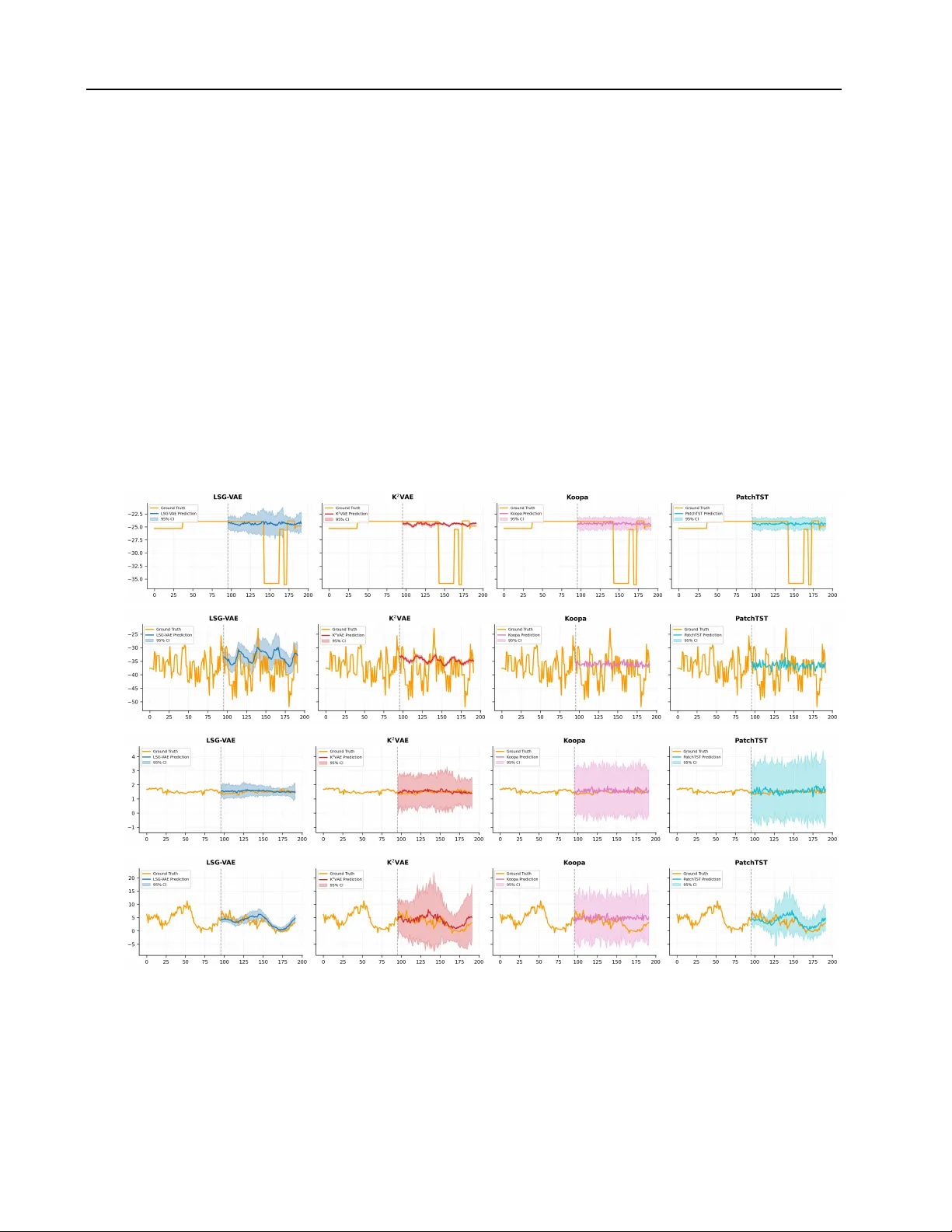
Embracing Heter oscedasticity f or Pr obabilistic T ime Series F or ecasting Y ijun W ang 1 Qiyuan Zhuang 1 Xiu-Shen W ei 1 Abstract Probabilistic time series forecasting (PTSF) aims to model the full predictiv e distrib ution of fu- ture observ ations, enabling both accurate fore- casting and principled uncertainty quantiﬁcation. A central requirement of PTSF is to embrace heteroscedasticity , as real-world time series ex- hibit time-varying conditional variances induced by nonstationary dynamics, regime changes, and ev olving e xternal conditions. Ho we ver , most ex- isting non-autoregressi v e generati ve approaches to PTSF , such as TimeV AE and K 2 V AE, rely on MSE-based training objecti ves that implicitly impose a homoscedastic assumption, thereby fun- damentally limiting their ability to model tem- poral heteroscedasticity . T o address this limi- tation, we propose the Location-Scale Gaussian V AE (LSG-V AE), a simple but effecti ve frame- work that e xplicitly parameterizes both the predic- tiv e mean and time-dependent variance through a location-scale likelihood formulation. This de- sign enables LSG-V AE to faithfully capture het- eroscedastic aleatoric uncertainty and introduces an adaptiv e attenuation mechanism that automati- cally do wn-weights highly v olatile observ ations during training, leading to improv ed robustness in trend prediction. Extensi ve e xperiments on nine benchmark datasets demonstrate that LSG-V AE consistently outperforms ﬁfteen strong generative baselines while maintaining high computational efﬁcienc y suitable for real-time deployment. 1 Introduction In recent years, deep learning has dri ven a paradigm shift in time series analysis ( Lim & Zohren , 2021 ; Kong et al. , 2025 ), achieving substantial progress in tasks ranging from imputation ( Cao et al. , 2018 ; T ashiro et al. , 2021 ; Gao et al. , 2025 ; W ang et al. , 2025 ; 2024b ) to anomaly detection ( Xu 1 Department of Computer Science, Southeast Univ er - sity , Nanjing, China. Correspondence to: Xiu-Shen W ei < weixs@seu.edu.cn > . Pr eprint. Mar ch 26, 2026. (a) Homoscedastic model (poor) Assumes constant variance Gr ound T ruth P r ediction Confidence Interval (b) Heter oscedastic model (good) Captur es time- varying uncertainty Gr ound T ruth P r ediction Confidence Interval F igur e 1. Homoscedastic vs. Heteroscedastic Forecasting. (a) Standard MSE-based models assume constant variance, leading the mean predictor to ﬁt transient ﬂuctuations. (b) LSG-V AE models time-varying uncertainty , allowing the mean prediction to focus on the underlying trend. et al. , 2022 ; W ang et al. , 2023 ; Liu & Paparrizos , 2024 ; Miao et al. , 2025 ; W u et al. , 2025b ). Among these, Prob- abilistic T ime Series Forecasting (PTSF) stands out as a critical capability for high-stakes decision-making ( Gneit- ing & Raftery , 2007 ; Gneiting et al. , 2007 ). In energy grids, probabilistic load forecasting is essential for risk-aware dis- patch ( Hong & Fan , 2016 ; W ang et al. , 2024a ; Sun et al. , 2022 ); in quantitative ﬁnance and supply chains, accurate uncertainty modeling supports robust risk control under volatility ( Sezer et al. , 2020 ; Li et al. , 2018 ; Huang et al. , 2022 ). Unlike deterministic forecasters that yield only point estimates, PTSF aims to model the full predictiv e distri- bution, allowing for the precise evaluation of conﬁdence intervals and tail risks ( Zhang et al. , 2024 ). Despite the gro wing interest, capturing the intrinsic het- eroscedasticity of real-world time series, characterized by conditional v ariances that ﬂuctuate dynamically ov er time, remains a formidable challenge ( Gneiting & Raftery , 2007 ). For instance, wind po wer generation exhibits stable patterns during calm weather but undergoes violent ﬂuctuations dur - ing storms; similarly , ﬁnancial markets alternate between periods of tranquility and b ursts of e xtreme v olatility during crises. A critical theoretical ov ersight persists in pre v alent non-autoregressi v e generati ve forecasting paradigms, such as standard V AEs ( Kingma & W elling , 2014 ; Desai et al. , 2021 ) and K 2 V AE ( W u et al. , 2025a ): they predominantly rely on the Mean Squared Error (MSE) objectiv e. Mathe- matically , minimizing MSE imposes a rigid homoscedastic assumption ( σ 2 = const ) ( Kendall & Gal , 2017 ). This as- 1 Embracing Heteroscedasticity f or Pr obabilistic Time Series F or ecasting sumption fundamentally mismatches the intrinsic nature of real-world data, which is characterized by dynamic, input- dependent volatility . As illustrated in Figure 1 (a), when confronted with volatile observations, such models lack an explicit mechanism to decouple the underlying trend from aleatoric uncertainty . Consequently , the MSE objective disproportionately penal- izes high-v ariance ﬂuctuations, rendering the mean predic- tor susceptible to overﬁtting these stochastic de viations and resulting in degraded generalization. T o address these limitations, we advocate a simple but ef- fectiv e philosophy: the difﬁculty often lies not in modeling increasingly complex latent dynamics, but in the lack of explicit mechanisms to decouple underlying trends from transient v olatility . Rather than introducing computationally heavy iterative generative procedures or relying on rigid MSE-based objectiv es, we ask: Can a lightweight gener- ative model be explicitly empower ed to know when to be uncertain? Motiv ated by this intuition, we propose the Location-Scale Gaussian V ariational Autoencoder (LSG-V AE). LSG-V AE bridges the gap between efﬁcienc y and probabilistic rigor . It adopts a non-autoregressiv e formulation to av oid error accumulation, while replacing the MSE surrogate with a principled location-scale likelihood. This formulation nat- urally induces an adapti ve attenuation ef fect (visualized in Figure 1 (b)). By dynamically estimating a time-dependent vari ance σ t , the model yields conﬁdence interv als with time- varying widths. From an optimization perspecti ve, this corresponds to down-weighting the contribution of high- variance observations ( ∝ 1 /σ 2 t ) in the loss function. As a result, the scale component captures irreducible stochas- tic uncertainty , allowing the location component to remain stable and recover the underlying trend without being domi- nated by outliers. In summary , LSG-V AE pro vides a streamlined frame work for ef ﬁcient and rob ust probabilistic forecasting. By emplo y- ing a global latent dynamics module, the model captures long-term dependencies in a single forw ard pass, a voiding the recursi ve pitf alls of autoregressi v e architectures. Com- pared to diffusion-based approaches that rely on expensi v e iterati ve denoising ( Rasul et al. , 2021a ; Shen & Kwok , 2023 ; Y e et al. , 2025 ), LSG-V AE achie ves substantially f aster infer- ence while maintaining competiti v e predicti ve uncertainty modeling. The main contributions of this work are as fol- lows: • Uniﬁed Non-autoregressi ve Framework: W e pro- pose LSG-V AE, a streamlined framework that in- tegrates a location-scale likelihood into a non- autoregressi v e architecture. This design not only cir- cumvents the error accumulation of autoregressiv e models but also introduces an intrinsic adapti ve at- tenuation mechanism, enabling the model to dynami- cally do wn-weight high-v ariance observ ations and ro- bustly decouple underlying trends from irreducible un- certainty . • Universality of the LSG Paradigm: W e validate that our proposed heteroscedastic modeling princi- ple is model-agnostic and transferable. By extending the LSG mechanism to other generative backbones, such as GAN-based (T imeGAN) and K oopman-based ( K 2 V AE) models, we demonstrate that this simple but effecti v e philosophy consistently enhances probabilis- tic forecasting performance across di verse architec- tures. • Strong P erf ormance and Efﬁciency: Extensive e xper- iments on 9 real-world benchmarks demonstrate that LSG-V AE consistently outperforms a wide range of strong baselines in both predictive accurac y and uncer- tainty calibration, while achie ving signiﬁcantly lo wer inference latency . W e release our code at https: //anonymous.4open.science/r/LSG- VAE . 2 Methodology 2.1 Problem F ormulation and Moti vation 2 . 1 . 1 P RO B A B I L I S T I C F O R E C A S T I N G F O R M U L A T I O N W e consider a multi v ariate time series forecasting scenario. Let X = { x t } L t =1 denote the historical look-back windo w of length L , where x t ∈ R C represents the observed v alues of C variables at time step t . The objective is to model the conditional probability density of the future horizon Y = { x t } L + H t = L +1 of length H : p θ ( Y | X ) . (1) Unlike deterministic approaches that yield a single point estimate ˆ Y ≈ E [ Y | X ] (often minimizing L 2 distance), our goal is to capture the full predicti v e distribution. This formu- lation is essential for quantifying the aleatoric uncertainty intrinsic to the data generation process, speciﬁcally the time- varying v olatility (heteroscedasticity). 2 . 1 . 2 T H E H O M O S C E DA S T I C T R A P I N V A N I L L A V A E S The V ariational Autoencoder (V AE) ( Kingma & W elling , 2014 ) provides a powerful framework for this generativ e task by introducing a latent variable Z . Howe ver , a criti- cal limitation in pre v alent time series V AEs is the implicit assumption of a ﬁxed-variance Gaussian likelihood for the decoder: p θ ( X | Z ) = N ( X ; µ θ ( Z ) , σ 2 const I ) . (2) 2 Embracing Heteroscedasticity f or Pr obabilistic Time Series F or ecasting Encoder Backbone 2. P a t c h - ba se d Va r i a t i o n a l E n c o d e r Repar amet eriza tion Tr i c k Sampl ing St ochas ti c Lat ent 3. N on - au tor egressive La tent - Dynam i cs Fl a ttened MLP Glob al Tra n s f o r m at i o n Fu ture Lat ent 4. Loc a tio n - Sc al e D eco der Loss Function Sc al e Head ( Unc ert ainty ) Sof tpl us (+ s t abili ty ) Loca tio n Head (T r en d) RevIN -1 ( DeNor m ) Pre dic tive Mean Pre dic tive Sc al e Predictive Distribution Adap tive Att enu a tion Mechanism Reshape d 1. Pre proce ssin g & Patc h i n g RevIN (Nor ma l iza t ion ) Patc h i n g Opera tio n Channe ls C Lookback Length L Inpu t Time Serie s KL Regu l ar iza t ion 𝜉 (𝐸 ! ) (𝐷 " ) (ℒ !"" ) Spl i t ℒ !"# + ℒ $!"% 𝜇 $!"% 𝜎 $!"% 𝒁 $&'( 𝒁 )*(*!" 𝜖 ～ Ν(0, 𝐼) 𝒁 $& ' ( Shared Deco der MLP 𝞵 MLP 𝞼 F igur e 2. Ov ervie w of the LSG-V AE Framework. The model se gments the input series into patches, encodes them into a probabilistic latent space, e v olves the state via ef ﬁcient global dynamics, and decodes the future using a dual-head mechanism to jointly predict location ( µ ) and scale ( σ ). Under this assumption, maximizing the Evidence Lower Bound (ELBO) in volv es maximizing the log-likelihood term, which mathematically de generates into the MSE ob- jectiv e: log p θ ( X | Z ) ∝ − X t ∥ x t − µ t ( Z ) ∥ 2 2 . (3) While computationally con v enient, this deri v ation exposes a rigid homoscedastic inducti ve bias: the model implicitly assumes that uncertainty remains constant across time steps. Consequently , the vanilla V AE tends to behave similarly to a deterministic regressor , limiting its ability to represent time-varying uncertainty in real-w orld systems. 2.2 The LSG-V AE Framework T o ov ercome the limitations of the homosceda stic assump- tion, we present the Location-Scale Gaussian V AE (LSG- V AE), a generative frame work designed to facilitate the modeling of global temporal dynamics separately from in- stantaneous local volatility . As depicted in Figure 2 , the architecture is composed of three integral modules: (1) a P atch-based V ariational Encoder responsible for extracting local semantic contexts; (2) a Non-autor e gr essive Latent Dynamics module that efﬁciently e v olves the temporal state; and (3) a Location-Scale Pr obabilistic Decoder that param- eterizes the ﬁnal predictiv e distrib ution. 2 . 2 . 1 P A T C H I N G A N D V A R I A T I O NA L E N C O D I N G T o alleviate the computational bottlenecks of point-wise processing and to better capture local semantic structures, we employ a patching strategy ( Nie et al. , 2023 ). W e ﬁrst apply Re versible Instance Normalization (Re vIN) to the input X to mitigate non-stationarity ( Kim et al. , 2022 ). The normalized series is then segmented into N non-ov erlapping patches P ∈ R N × P × C , where P denotes the patch length. The encoder E ϕ maps these patches into a stochastic la- tent space. Follo wing the variational autoencoder frame- work ( Kingma & W elling , 2014 ), we model the posterior distribution of the past latent states Z past as a diagonal Gaussian to account for epistemic uncertainty arising from noisy observations: q ϕ ( Z past | P ) = N ( µ z , σ 2 z ) . (4) Here, ( µ z , σ z ) = E ϕ ( P ) . Utilizing the reparameteriza- tion trick ( Kingma & W elling , 2014 ), we sample Z past = µ z + ϵ ⊙ σ z , where ϵ ∼ N (0 , I ) . This stochastic injection regularizes the latent representation and improves robust- ness to input perturbations. 2 . 2 . 2 N O N - AU T O R E G R E S S I V E L A T E N T D Y N A M I C S Modeling the transition from past latent representations Z past to future representations Z f uture is a critical compo- nent. While recurrent architectures (e.g., RNNs) are capable of sequential modeling, they are prone to error accumula- tion and suf fer from high latenc y in long-horizon forecast- ing ( Bengio et al. , 2015 ). T o address this limitation, we propose a lightweight Non-autoregressi ve Latent Dynamics mechanism. W e adopt the modeling assumption that the high-lev el se- mantic evolution of a time series can be approximated by a global transformation in the latent space. Speciﬁcally , we ﬂatten the past latent representations and project them 3 Embracing Heteroscedasticity f or Pr obabilistic Time Series F or ecasting directly to the future horizon: Z f uture = Pro jection(Flatten( Z past )) ∈ R M × D , (5) where M denotes the number of future patches. This non- autoregressi v e design enables the model to capture global temporal dependencies and generate the entire future hori- zon in a single forward pass. This parallel decoding mecha- nism eliminates the computational bottleneck of recursive generation, resulting in improv ed computational ef ﬁciency compared to autoregressi ve probabilistic forecasters such as DeepAR ( Salinas et al. , 2020 ) and T imeGrad ( Rasul et al. , 2021a ). 2 . 2 . 3 L O C A T I O N - S C A L E P R O BA B I L I S T I C D E C O D I N G This module constitutes the core mechanism for capturing intrinsic heteroscedasticity . Con ventional V AEs for time series typically utilize a single-head decoder , implicitly as- suming a ﬁx ed-v ariance Gaussian likelihood. W e contend that this assumption is often inadequate for real-world data exhibiting dynamic volatility . T o address this limitation, we introduce a shared Dual-Head Decoder D ψ . This decoder operates with identical weights on both the historical latent representations Z past and the future latent representations Z f uture , ensuring a consistent mapping from latent space to the observation space. In terms of implementation, we do not employ two sepa- rate networks. Instead, we use a single MLP backbone to project the latent states. The output of this MLP is then split along the last dimension to decouple the location and scale parameters simultaneously . The ﬁrst part of the split serves as the Location Head, capturing the central tendency (trend and seasonality). T o restore the original scale of the data, the in v erse Re vIN operation is applied: µ = RevIN − 1 ( MLP µ ( Z )) . (6) The second part constitutes the Scale Head , estimating the instantaneous volatility (aleatoric uncertainty). T o ensure numerical stability and strictly positiv e standard de viations, we model the log-variance via a Softplus acti v ation: σ = Softplus ( MLP σ ( Z )) + ξ , (7) where ξ is a small stability constant (e.g., 10 − 6 ). Crucially , this dual-head mechanism empo wers the model to rigorously capture the residual uncertainty that remains unexplained by the location estimate in both historical and future contexts. 2 . 2 . 4 O B J E C T I V E F U N C T I O N : E M B R A C I NG H E T E RO S C E D A S T I C I T Y The training objecti ve is to maximize the Evidence Lo wer Bound (ELBO). Unlike many forecasting-oriented V AE variants that rely on MSE-based reconstruction objecti v es, we reformulate the objective to explicitly account for het- eroscedasticity in both reconstruction and prediction phases. The Composite Location-Scale Loss. W e adopt the Gaus- sian Negati v e Log-Likelihood (NLL) for both the look-back windo w reconstruction ( L rec ) and the future horizon predic- tion ( L pred ). The total loss function L is deﬁned as: L = L rec ( X ) | {z } Reconstruction + L pred ( Y ) | {z } Prediction + β · D K L ( q ϕ ( Z past | P ) ∥ N (0 , I )) . (8) Both L rec and L pred are computed using the heteroscedastic Gaussian NLL. F or a generic sequence u of length T (where u is x or y ), the loss is: L NLL ( u ) = 1 T C X t,c log σ t,c + ( u t,c − µ t,c ) 2 2 σ 2 t,c ! . (9) By jointly minimizing L rec and L pred , the model is forced to learn a latent representation that is both descriptiv e of historical patterns and predictiv e of future dynamics. Theoretical Analysis (Adapti ve Attenuation). The gradi- ent of the NLL term rev eals an adaptiv e attenuation mecha- nism: ∇ µ L N LL ∝ 1 σ 2 ( u − µ ) . (10) When the model encounters an outlier or high volatility in the history (reconstruction) or uncertain future regimes (prediction), it learns to increase σ . This effecti v ely do wn- weights the gradient contribution of that speciﬁc point ( 1 σ 2 → 0 ), prev enting the Location Head from overﬁtting to transient stochastic ﬂuctuations. This mechanism trans- forms the model from a passi ve curve ﬁtter into an active risk estimator . For a rigorous mathematical deri v ation of the heteroscedastic ELBO and a formal proof of this attenuation mechanism, please refer to the detailed theoretical analysis in Appendix B . 3 Experiments on Synthetic Data In real-world empirical studies, the true aleatoric uncertainty is inherently latent and unobserv able, making it dif ﬁcult to rigorously verify whether a model is capturing volatility dynamics or merely overﬁtting residual artifacts ( K endall & Gal , 2017 ). T o address this, we validate the heteroscedas- tic modeling capability of LSG-V AE within a controlled analytical en vironment where both the underlying trend and the v olatility proﬁle are mathematically deﬁned and known ( Gal & Ghahramani , 2016 ). This experiment serves as a critical veriﬁcation of our Location–Scale formulation: the model must demonstrate the ability to disentangle the deterministic signal, modeled by the Location Head, from the time-varying v olatility , captured by the Scale Head. 4 Embracing Heteroscedasticity f or Pr obabilistic Time Series F or ecasting Data Generating Process W e analyze uni v ariate se- quences governed by the process y t = µ t + ϵ t , where the underlying deterministic trend is deﬁned as µ t = sin( t ) and the stochastic term follows ϵ t ∼ N (0 , σ 2 t ) . T o stress-test the model under extreme heteroscedasticity , we introduce two distinct volatility proﬁles as illustrated in Figure 3 . The ﬁrst is a Re gime-Switching scenario (T op Row), which simulates structural breaks by having σ t alternate abruptly between stable ( 0 . 1 ) and high-v olatility ( 1 . 0 ) states, thereby challeng- ing the model’ s adaptability to sudden distributional shifts. The second is a Periodic pattern (Bottom Row), deﬁned by a continuous v olatility trajectory σ t = 0 . 5 + 0 . 4 cos( t ) ; this proﬁle is deliberately phase-shifted relati v e to the mean to rigorously test the model’ s ability to decouple correlated but distinct dynamics. Results and Analysis Figure 3 visualizes the forecasting and v ariance reco v ery performance, conﬁrming LSG-V AE’ s ﬁdelity in reconstructing latent heteroscedastic dynamics. In the Regime-Switching scenario (a-b), the predicted scale ˆ σ t tightly tracks the ground-truth step function with high correlation ( ρ = 0 . 985 ). This precise estimation allows the conﬁdence intervals to e xhibit a distinct “breathing” beha v- ior—instantly expanding during v olatility spik es to encap- sulate noise and contracting during stable periods—without distorting the trend prediction. Similarly , in the Periodic scenario (c-d), the model achiev es near-perfect disentangle- ment ( ρ = 0 . 999 ), effecti v ely distinguishing the signal’ s phase from the cycl ic volatility proﬁle. Crucially , these re- sults demonstrate that the Location and Scale heads hav e successfully specialized in their respectiv e roles, transform- ing the model from a passiv e curv e ﬁtter into an activ e risk estimator that separates what is predicted (trend) from what is uncertain (volatility). 4 Experiments on Real-W orld Data W e conduct extensi v e experiments to comprehensi vely e v al- uate the effecti veness, robustness, and generalizability of LSG-V AE. Our e v aluation focuses on large-scale real-world probabilistic time series forecasting tasks, followed by abla- tion studies, qualitati v e analysis, generalization experiments, and efﬁcienc y comparisons. T o rigorously ev aluate LSG-V AE against SOT A methods, we conduct extensiv e experiments under two established ev aluation protocols. First, we follow the comprehensive benchmarking setting introduced in ProbTS ( Zhang et al. , 2024 ), which provides a uniﬁed frame w ork for comparing both point and probabilistic time series forecasters under standard accuracy metrics ( Zhang et al. , 2024 ). In addition, we align this setting with recent V AE-based generativ e fore- casting work, such as K 2 V AE, to ensure fair comparison across deterministic and probabilistic models ( W u et al. , 2025a ). Second, we adopt the e xperimental protocol com- F igur e 3. Qualitati v e results on synthetic datasets. Left: forecast- ing with adaptiv e 95% conﬁdence interv als under v arying v olatil- ity . Right: uncertainty recovery , where the predicted v olatility ˆ σ t closely matches the ground truth. monly used by recent SO T A diffusion models for time series forecasting, which focuses on probabilistic calibration and distributional quality , as exempliﬁed by NsDiff ( Y e et al. , 2025 ). 4.1 Evaluation under the K 2 V AE Protocol Datasets W e conduct experiments on nine widely- recognized real-w orld benchmarks from ProbTS ( Zhang et al. , 2024 ), spanning div erse domains: Energy ( ETTh1 , ETTh2 , ETTm1 , ETTm2 , Electricity ), T ransportation ( T raf- ﬁc ), W eather ( W eather ), Economics ( Exchange ), and Health ( ILI ). Follo wing the standard protocol for long-term fore- casting, we set the look-back windo w length to L = 96 for all datasets, except for ILI where L = 36 . The forecasting horizons are set to H ∈ { 96 , 192 , 336 , 720 } for the general datasets and H ∈ { 24 , 36 , 48 , 60 } for ILI . Baselines W e compare LSG-V AE with 11 competitive baselines, co vering both deterministic and probabilistic fore- casting paradigms. Speciﬁcally , the selected baselines in- clude deep point forecasters such as FITS ( Xu et al. , 2024 ), PatchTST ( Nie et al. , 2023 ), iT ransformer ( Liu et al. , 2024 ), and K oopa ( Liu et al. , 2023 ), which are originally designed for deterministic prediction. For fair probabilistic ev aluation, these models are augmented with a Gaussian output head to predict distribution parameters ( µ, σ ) . In addition, we con- sider a broad range of probabilistic and generati v e models, including TSDiff ( K ollovieh et al. , 2023 ), T imeGrad ( Ra- sul et al. , 2021a ), CSDI ( T ashiro et al. , 2021 ), GR U NVP , GR U MAF , Trans MAF ( Rasul et al. , 2021b ), as well as K 2 V AE ( W u et al. , 2025a ). Implementation details are provided in Appendix C.4 . Metrics W e employ two complementary metrics: Continu- ous Ranked Probability Score (CRPS) to measure the distri- butional ﬁt and Normalized Mean Absolute Error (NMAE) to assess point prediction accurac y . Lower v alues indicate better performance for both metrics. Detailed descriptions 5 Embracing Heteroscedasticity f or Pr obabilistic Time Series F or ecasting T able 1. Comparison on long-term probabilistic forecasting (forecasting horizon L=720) scenarios across nine real-world datasets. Lower CRPS or NMAE values indicate better predictions. The means and standard errors are based on 5 independent runs of retraining and ev aluation. Red : the best, Blue : the 2nd best. The full results of all four horizons 96, 192, 336, 720 are listed in T able 6 , 7 in Appendix C.5 . Model Metric ETTm1 ETTm2 ETTh1 ETTh2 Electricity T rafﬁc W eather Exchange ILI FITS CRPS 0 . 305 ± 0 . 024 0 . 449 ± 0 . 034 0 . 348 ± 0 . 025 0 . 314 ± 0 . 022 0 . 115 ± 0 . 024 0 . 374 ± 0 . 004 0 . 267 ± 0 . 003 0 . 074 ± 0 . 011 0 . 211 ± 0 . 011 NMAE 0 . 406 ± 0 . 072 0 . 540 ± 0 . 052 0 . 468 ± 0 . 012 0 . 401 ± 0 . 022 0 . 149 ± 0 . 012 0 . 453 ± 0 . 022 0 . 317 ± 0 . 021 0 . 097 ± 0 . 011 0 . 245 ± 0 . 017 PatchTST CRPS 0 . 304 ± 0 . 029 0 . 229 ± 0 . 036 0 . 323 ± 0 . 020 0 . 304 ± 0 . 018 0 . 127 ± 0 . 015 0 . 214 ± 0 . 001 0 . 142 ± 0 . 005 0 . 097 ± 0 . 007 0 . 233 ± 0 . 019 NMAE 0 . 382 ± 0 . 066 0 . 288 ± 0 . 034 0 . 428 ± 0 . 024 0 . 371 ± 0 . 021 0 . 164 ± 0 . 024 0 . 253 ± 0 . 012 0 . 152 ± 0 . 029 0 . 126 ± 0 . 001 0 . 287 ± 0 . 023 iT ransformer CRPS 0 . 455 ± 0 . 021 0 . 311 ± 0 . 024 0 . 350 ± 0 . 019 0 . 542 ± 0 . 015 0 . 109 ± 0 . 044 0 . 284 ± 0 . 004 0 . 133 ± 0 . 004 0 . 087 ± 0 . 023 0 . 222 ± 0 . 020 NMAE 0 . 490 ± 0 . 038 0 . 385 ± 0 . 042 0 . 449 ± 0 . 022 0 . 667 ± 0 . 012 0 . 140 ± 0 . 009 0 . 361 ± 0 . 030 0 . 147 ± 0 . 019 0 . 113 ± 0 . 015 0 . 278 ± 0 . 017 K oopa CRPS 0 . 295 ± 0 . 027 0 . 233 ± 0 . 025 0 . 318 ± 0 . 009 0 . 293 ± 0 . 026 0 . 113 ± 0 . 018 0 . 358 ± 0 . 022 0 . 140 ± 0 . 007 0 . 091 ± 0 . 012 0 . 228 ± 0 . 022 NMAE 0 . 377 ± 0 . 037 0 . 290 ± 0 . 033 0 . 412 ± 0 . 008 0 . 286 ± 0 . 042 0 . 149 ± 0 . 025 0 . 432 ± 0 . 032 0 . 162 ± 0 . 009 0 . 116 ± 0 . 022 0 . 288 ± 0 . 031 TSDiff CRPS 0 . 478 ± 0 . 027 0 . 344 ± 0 . 046 0 . 516 ± 0 . 027 0 . 406 ± 0 . 056 0 . 478 ± 0 . 005 0 . 391 ± 0 . 002 0 . 152 ± 0 . 003 0 . 082 ± 0 . 010 0 . 263 ± 0 . 022 NMAE 0 . 622 ± 0 . 045 0 . 416 ± 0 . 065 0 . 657 ± 0 . 017 0 . 482 ± 0 . 022 0 . 622 ± 0 . 142 0 . 478 ± 0 . 006 0 . 141 ± 0 . 026 0 . 142 ± 0 . 009 0 . 272 ± 0 . 020 GR U NVP CRPS 0 . 546 ± 0 . 036 0 . 561 ± 0 . 273 0 . 502 ± 0 . 039 0 . 539 ± 0 . 090 0 . 114 ± 0 . 013 0 . 211 ± 0 . 004 0 . 110 ± 0 . 004 0 . 079 ± 0 . 009 0 . 307 ± 0 . 005 NMAE 0 . 707 ± 0 . 050 0 . 749 ± 0 . 385 0 . 643 ± 0 . 046 0 . 688 ± 0 . 161 0 . 144 ± 0 . 017 0 . 264 ± 0 . 006 0 . 135 ± 0 . 008 0 . 103 ± 0 . 009 0 . 333 ± 0 . 005 GR U MAF CRPS 0 . 536 ± 0 . 033 0 . 272 ± 0 . 029 0 . 393 ± 0 . 043 0 . 990 ± 0 . 023 0 . 106 ± 0 . 007 - 0 . 122 ± 0 . 006 0 . 160 ± 0 . 019 0 . 172 ± 0 . 034 NMAE 0 . 711 ± 0 . 081 0 . 355 ± 0 . 048 0 . 496 ± 0 . 019 1 . 092 ± 0 . 019 0 . 136 ± 0 . 098 - 0 . 149 ± 0 . 034 0 . 182 ± 0 . 010 0 . 216 ± 0 . 014 T rans MAF CRPS 0 . 688 ± 0 . 043 0 . 355 ± 0 . 043 0 . 363 ± 0 . 053 0 . 327 ± 0 . 033 - - 0 . 113 ± 0 . 004 0 . 148 ± 0 . 017 0 . 155 ± 0 . 018 NMAE 0 . 822 ± 0 . 034 0 . 475 ± 0 . 029 0 . 455 ± 0 . 025 0 . 412 ± 0 . 020 - - 0 . 148 ± 0 . 040 0 . 191 ± 0 . 006 0 . 183 ± 0 . 019 T imeGrad CRPS 0 . 621 ± 0 . 037 0 . 470 ± 0 . 054 0 . 523 ± 0 . 027 0 . 445 ± 0 . 016 0 . 108 ± 0 . 003 0 . 220 ± 0 . 002 0 . 113 ± 0 . 011 0 . 099 ± 0 . 015 0 . 295 ± 0 . 083 NMAE 0 . 793 ± 0 . 034 0 . 561 ± 0 . 044 0 . 672 ± 0 . 015 0 . 550 ± 0 . 018 0 . 134 ± 0 . 004 0 . 263 ± 0 . 001 0 . 136 ± 0 . 020 0 . 113 ± 0 . 016 0 . 325 ± 0 . 068 CSDI CRPS 0 . 448 ± 0 . 038 0 . 239 ± 0 . 035 0 . 528 ± 0 . 012 0 . 302 ± 0 . 040 - - 0 . 087 ± 0 . 003 0 . 143 ± 0 . 020 0 . 283 ± 0 . 012 NMAE 0 . 578 ± 0 . 051 0 . 306 ± 0 . 040 0 . 657 ± 0 . 014 0 . 382 ± 0 . 030 - - 0 . 102 ± 0 . 005 0 . 173 ± 0 . 020 0 . 299 ± 0 . 013 K 2 V AE CRPS 0 . 294 ± 0 . 026 0 . 221 ± 0 . 023 0 . 314 ± 0 . 011 0 . 280 ± 0 . 014 0 . 087 ± 0 . 005 0 . 200 ± 0 . 001 0 . 084 ± 0 . 003 0 . 069 ± 0 . 005 0 . 142 ± 0 . 008 NMAE 0 . 373 ± 0 . 032 0 . 275 ± 0 . 035 0 . 396 ± 0 . 012 0 . 278 ± 0 . 020 0 . 117 ± 0 . 019 0 . 248 ± 0 . 010 0 . 099 ± 0 . 009 0 . 084 ± 0 . 017 0 . 167 ± 0 . 007 LSG-V AE ∗ CRPS 0.279 ± 0 . 020 0.166 ± 0 . 018 0.310 ± 0 . 012 0.174 ± 0 . 010 0.080 ± 0 . 006 0.192 ± 0 . 003 0.073 ± 0 . 003 0.065 ± 0 . 004 0.130 ± 0 . 005 NMAE 0.367 ± 0 . 023 0.207 ± 0 . 026 0.389 ± 0 . 013 0.223 ± 0 . 015 0.111 ± 0 . 012 0.236 ± 0 . 009 0.086 ± 0 . 006 0.077 ± 0 . 012 0.155 ± 0 . 006 ∗ indicates that LSG-V AE signiﬁcantly outperforms K 2 V AE under paired W ilcoxon signed-rank tests ( p < 0 . 05 ). of these metrics can be found in Appendix C.3 . Results and Analysis T able 1 summarizes the performance for the challenging long-term horizon ( H = 720 ). A sig- niﬁcant and counter-intuiti v e ﬁnding is that LSG-V AE con- sistently outperforms specialized point forecasters, such as PatchTST and iT ransformer , even on the deterministic met- ric (NMAE). This empirically conﬁrms that explicitly mod- eling heteroscedasticity enables the NLL objecti ve to adap- tiv ely do wn-weight noisy samples, ef fecti vely rob ustifying the mean predictor against outliers. Furthermore, compared to the previous SOT A V AE-based method, K 2 V AE, our model achiev es consistent improv ements across all datasets. This highlights that the simple, principled Location-Scale paradigm offers a more effecti ve approach for time series modeling than complex reconstruction schemes. 4.2 Evaluation under the NsDiff Pr otocol Datasets T o assess generativ e capability , we follow the speciﬁc protocol used in recent diffusion-based studies. W e utilize 8 datasets: ETT (m1, m2, h1, h2), Electricity , T r af ﬁc , Exchange , and ILI . Consistent with this protocol, the input length is ﬁxed at L = 168 (except ILI). Baselines W e compare against 6 advanced generati v e base- lines, including the classic autore gressiv e dif fusion model T imeGrad ( Rasul et al. , 2021a ) and SO T A dif fusion-based approaches, namely CSDI ( T ashiro et al. , 2021 ), TimeD- iff ( Shen & Kwok , 2023 ), Dif fusionTS ( Y uan & Qiao , 2024 ), TMDM ( Li et al. , 2024 ), and NsDiff ( Y e et al. , 2025 ). Metrics In addition to CRPS, we employ the Quantile In- terval Calibration Error (QICE) to strictly e v aluate the cali- bration quality of the predicted conﬁdence intervals. QICE measures the discrepancy between the empirical and nomi- nal cov erage probabilities, where a lo wer v alue indicates a more trustworthy uncertainty estimation. Detailed descrip- tions of these metrics can be found in Appendix C.3 . Results and Analysis As shown in T able 2 , LSG-V AE demonstrates remarkable performance against competiti v e generativ e baselines. In terms of probabilistic performence, LSG-V AE achieves the best CRPS across all eight datasets, signiﬁcantly outperforming recent SO T A diffusion models. This result is particularly notable gi v en the ef ﬁcienc y gap: while dif fusion-based approaches like CSDI and NsDiff require computationally expensi v e iterati ve denoising steps to reconstruct distributions, LSG-V AE achie v es superior modeling quality in a single non-autore gressi ve forward pass. Furthermore, regarding calibration quality , LSG-V AE ranks either ﬁrst or second in terms of QICE across the majority of datasets. This indicates that the conﬁdence intervals generated by our Location-Scale decoder are not only accurate b ut also well-calibrated, f aithfully reﬂecting the true aleatoric uncertainty of the data without the need for complex iterati v e reﬁnement. 4.3 Ablation Studies T o thoroughly in vestigate the contrib ution of each compo- nent in our training objectiv e, we conduct a component- wise ablation study . The total loss is deﬁned as L = 6 Embracing Heteroscedasticity f or Pr obabilistic Time Series F or ecasting T able 2. Quantitati ve comparison of probabilistic forecasting on 8 real-world datasets( L = 168 , H = 192 ). Metrics: CRPS and QICE (lower is better). Red indicates the best performance, and Blue indicates the 2nd best. Model Metric ETTm1 ETTm2 ETTh1 ETTh2 Electricity T raf ﬁc Exchange ILI T imeGrad CRPS 0.647 0.775 0.606 1.212 0.397 0.407 0.826 1.140 QICE 6.693 6.962 6.731 9.488 7.118 4.581 9.464 6.519 CSDI CRPS 0.524 0.817 0.492 0.647 0.577 1.418 0.855 1.244 QICE 2.828 8.106 3.107 5.331 7.506 13.613 7.864 7.693 T imeDif f CRPS 0.464 0.316 0.465 0.471 0.750 0.771 0.433 1.153 QICE 14.795 13.385 14.931 14.813 15.466 15.439 14.556 14.942 DiffusionTS CRPS 0.574 1.035 0.603 1.168 0.633 0.668 1.251 1.612 QICE 5.605 9.959 6.423 9.577 8.205 5.958 10.411 10.090 TMDM CRPS 0.375 0.289 0.452 0.383 0.461 0.557 0.336 0.967 QICE 2.567 2.610 2.821 4.471 10.562 10.676 6.393 6.217 NsDiff CRPS 0.346 0.256 0.392 0.358 0.290 0.378 0.324 0.806 QICE 2.041 2.030 1.470 2.074 6.685 3.601 5.930 5.598 LSG-V AE CRPS 0.236 0.130 0.288 0.174 0.080 0.190 0.032 0.107 QICE 1.623 2.373 1.450 2.385 1.082 1.363 3.174 4.968 T able 3. Component-wise ablation on ETTh1 and Electricity . W e compare LSG-V AE with v ariants without prediction loss (w/o P), without reconstruction loss (w/o R), and a vanilla V AE (MSE). Metrics: CRPS and NMAE. Bold indicates the best result. Dataset Horizon CRPS ↓ NMAE ↓ V an. w/o P w/o R Ours V an. w/o P w/o R Ours ETTh1 96 0.287 0.374 0.277 0.252 0.329 0.464 0.354 0.328 192 0.323 0.378 0.282 0.277 0.368 0.470 0.370 0.365 336 0.352 0.386 0.305 0.300 0.388 0.486 0.395 0.384 720 0.355 0.393 0.318 0.310 0.396 0.504 0.398 0.389 Electricity 96 0.363 0.259 0.082 0.069 0.362 0.363 0.107 0.089 192 0.363 0.261 0.086 0.075 0.364 0.363 0.112 0.096 336 0.364 0.264 0.099 0.078 0.364 0.366 0.129 0.102 720 0.370 0.269 0.103 0.080 0.370 0.371 0.135 0.111 L rec + L pred + β D K L . W e measure performance using CRPS (probabilistic calibration) and NMAE (deterministic accuracy). W e compare the full LSG-V AE against three distinct variants: w/o Prediction ( L pred = 0 ), which is trained exclusi vely on reconstructing historical patches to test whether latent dynamics can be learned without future supervision; w/o Reconstruction ( L rec = 0 ), which removes the historical reconstruction loss to verify if the auxiliary reconstruction task aids in regularizing the latent space; and V anilla V AE (MSE), which replaces the heteroscedastic Location-Scale NLL with a standard homoscedastic MSE loss. The results on ETTh1 and Electricity , summarized in T a- ble 3 , validate the synergy of our proposed components. First, the w/o Pred variant exhibits the sharpest deterioration in deterministic accuracy , conﬁrming that explicit future supervision is indispensable for guiding the latent dynamics module. Similarly , the consistent performance drop in the w/o Rec v ariant indicates that historical reconstruction is essential for regularizing the latent space and prev enting ov erﬁtting. Crucially , the V anilla V AE signiﬁcantly lags behind LSG-V AE in probabilistic metrics. This empirically prov es that the homoscedastic bias inherent in the MSE ob- jectiv e se v erely limits uncertainty calibration, whereas our T able 4. Generalizability analysis on ETTh1 and W eather datasets ( L = 96 , H = 96 ). W e compare the standard MSE-based base- lines against our Location-Scale (LSG) v ariants. Bold indicates the better performance. Model Framew ork ETTh1 W eather CRPS ↓ NMAE ↓ CRPS ↓ NMAE ↓ Generative Adversarial Networks (GAN) T imeGAN 0.277 0.347 0.106 0.117 LSG-GAN (Ours) 0.262 0.339 0.068 0.081 V ariational A utoencoders (V AE) K 2 V AE 0.264 0.336 0.080 0.086 LSG- K 2 V AE (Ours) 0.251 0.332 0.065 0.076 Location-Scale formulation effecti v ely captures dynamic volatility . Additionally , while we observe that LSG-V AE is robust to the KL di v ergence term, we retain it to ensure the theoretical integrity of the v ariational frame work. Further- more, we extend our in vestigation to architectural design choices. Detailed ablation studies concerning the impact of RevIN are pro vided in Appendix C.6 . And hyperparameter sensitivity analysis can be found in the Appendix C.7 . 4.4 Generalizability Analysis A piv otal question remains: Is the effectiveness of the Location-Scale objective limited to our speciﬁc ar chi tec- tur e? T o demonstrate the uni v ersality of our heteroscedastic modeling paradigm, we extend the proposed principle to other generativ e frame works. Extension to GANs (LSG-GAN) T o verify the gener- ality of our approach beyond V AEs, we integrate the Location-Scale mechanism into the adversarial training framew ork. W e construct LSG-GAN by modifying the clas- sic T imeGAN architecture: the deterministic generator out- put is replaced with our dual-head parameterization, while the discriminator architecture remains unchanged. Crucially , the discriminator is trained to distinguish samples drawn 7 Embracing Heteroscedasticity f or Pr obabilistic Time Series F or ecasting ETTh1 F igur e 4. V isual comparison of probabilistic forecasting on ETTh1 . All subﬁgures share a uniﬁed Y -axis scale. Additional visualization results are provided in Appendix C.8 . F igur e 5. Efﬁciency vs. Performance comparison on ETTh2 ( L = 96 , H = 720 ). The bubble size indicates inference memory usage (smaller is better). from the predicted distribution N ( µ , σ 2 ) rather than deter- ministic point estimates, and the generator is supervised via the Gaussian NLL loss. As shown in T able 4 (T op), this sim- ple modiﬁcation consistently outperforms the MSE-based T imeGAN baseline on both ETTh1 and W eather datasets. These results suggest that explicitly modeling heteroscedas- tic uncertainty provides complementary beneﬁts to adver - sarial learning, enhancing distribution matching ev en in non-variational settings. Enhancing SO T A V AEs (LSG- K 2 V AE) W e further apply our paradigm to K 2 V AE, a SO T A method that originally relies on a deterministic reconstruction objectiv e. By simply replacing its MSE reconstruction loss with our Location- Scale NLL objectiv e—without an y architectural changes to its core dynamics—we deri v e an enhanced v ariant termed LSG- K 2 V AE. Quantitativ e comparisons in T able 4 (Bot- tom) rev eal that this “plug-and-play” modiﬁcation yields immediate performance gains. For instance, LSG- K 2 V AE achiev es a signiﬁcant reduction in CRPS on the W eather dataset, conﬁrming that our proposed paradigm serves as a robust, model-agnostic plugin for boosting probabilistic forecasting performance. 4.5 Qualitative Analysis W e visualize the forecasting results on ETTh1 ( L = 96 , H = 96 ) in Figure 4 , comparing LSG-V AE against the K 2 V AE and adv anced point forecasters equipped with prob- abilistic heads (Koopa, PatchTST). As illustrated, LSG-V AE demonstrates superior adaptability , eff ectiv ely capturing intrinsic volatility dynamics. Speciﬁcally , the conﬁdence intervals (CIs) generated by LSG-V AE are sharp and dy- namically responsiv e—the y expand during v olatile periods and contract in stable regimes. This stands in sharp contrast to the baselines, which suffer from sev ere uncertainty bloat- ing: K 2 V AE, Koopa, and PatchTST produce excessi v ely wide and nearly uniform intervals that fail to mimic the temporal rhythm of the data. This visual evidence conﬁrms that merely grafting a Gaussian head onto deterministic backbones or using standard reconstruction losses leads to under-conﬁdent estimation, whereas LSG-V AE successfully captures the dynamic heteroscedasticity . 4.6 Efﬁciency Analysis Beyond forecasting performance, computational ef ﬁciency is paramount for real-world deployment. W e e v aluate the in- ference latency (batch size=1) and memory usage on ETTh2 using a single NVIDIA R TX 4090, with 100 samples gener- ated for probabilistic baselines. As illustrated in Figure 5 , LSG-V AE achieves the optimal trade-of f between accurac y and speed. Unlike diffusion models that require hundreds of expensiv e iterativ e denoising steps, LSG-V AE gener- ates the entire future horizon in a single non-autoregressiv e forward pass. This structural advantage results in orders-of- magnitude faster inference and a signiﬁcantly lo wer mem- ory footprint, rendering LSG-V AE highly suitable for time- critical streaming applications. 5 Conclusions W e presented LSG-V AE, a streamlined non-autoregressi ve frame work designed to capture the dynamic heteroscedastic- ity inherent in real-world time series. Experiments conﬁrm that, by replacing the rigid MSE objectiv e with a Location- Scale likelihood, LSG-V AE establishes a ne w state-of-the- art balance between forecasting accuracy , uncertainty cali- bration, and computational ef ﬁcienc y . Moreover , the prov en univ ersality of the LSG mechanism suggests a promising direction for future probabilistic time series forecasting re- search : shifting focus from complex model design to theo- retically grounded uncertainty quantiﬁcation. 8 Embracing Heteroscedasticity f or Pr obabilistic Time Series F or ecasting Impact Statement This paper presents work whose goal is to advance the ﬁeld of Machine Learning. There are many potential societal consequences of our work, none which we feel must be speciﬁcally highlighted here. References Alexandro v , A., Benidis, K., Bohlke-Schneider , M., Flunkert, V ., Gasthaus, J., Januschowski, T ., Maddix, D. C., Rangapuram, S., Salinas, D., Schulz, J., Stella, L., T ¨ urkmen, A. C., and W ang, Y . GluonTS: Probabilis- tic and neural time series modeling in python. J . Mach. Learn. Res. , 21(116):1–6, 2020. Bengio, S., V inyals, O., Jaitly , N., and Shazeer , N. Sched- uled Sampling for Sequence Prediction with Recurrent Neural Networks. In Advances in Neural Inf. Pr ocess. Syst. , pp. 1171–1179, 2015. Cao, W ., W ang, D., Li, J., Zhou, H., Li, L., and Li, Y . BRITS: Bidirectional Recurrent Imputation for T ime Series. In Advances in Neural Inf. Pr ocess. Syst. , pp. 6776–6786, 2018. Desai, A., Freeman, C., W ang, Z., and Beaver , I. T imeV AE: A variational auto-encoder for multiv ariate time series generation. arXiv pr eprint arXiv:2111.08095 , 2021. Gal, Y . and Ghahramani, Z. Dropout as a Bayesian Ap- proximation: Representing Model Uncertainty in Deep Learning. In Pr oc. Int. Conf. Mach. Learn. , pp. 1050– 1059, 2016. Gao, H., Shen, W ., Qiu, X., Xu, R., Y ang, B., and Hu, J. SSD-TS: Exploring the Potential of Linear State Space Models for Diffusion Models in T ime Series Imputation. In Pr oc. A CM SIGKDD Int. Conf. Knowledge disco very & data mining , pp. 649–660, 2025. Gneiting, T . and Raftery , A. E. Strictly Proper Scoring Rules, Prediction, and Estimation. J. Amer . Statist. Assoc. , 102 (477):359–378, 2007. Gneiting, T ., Balabdaoui, F ., and Raftery , A. E. Probabilistic forecasts, calibration and sharpness. J ournal of the Royal Statistical Society Series B: Statistical Methodology , 69 (2):243–268, 2007. Gu, A. and Dao, T . Mamba: Linear -time sequence modeling with selecti ve state spaces. arXiv pr eprint arXiv:2312.00752 , 2023. Hong, T . and Fan, S. Probabilistic electric load forecasting: A tutorial revie w. Int. J. F or ecasting , 32(3):914–938, 2016. Huang, X., Y ang, Y ., W ang, Y ., W ang, C., Zhang, Z., Xu, J., Chen, L., and V azirgiannis, M. DGraph: A Large- Scale Financial Dataset for Graph Anomaly Detection. In Advances in Neural Inf. Pr ocess. Syst. , pp. 22765–22777, 2022. Kendall, A. and Gal, Y . What uncertainties do we need in bayesian deep learning for computer vision? In Advances in Neural Inf . Pr ocess. Syst. , pp. 5580–5590, 2017. Kim, T ., Kim, J., T ae, Y ., Park, C., Choi, J., and Jaegul, C. Rev ersible Instance Normalization for Accurate Time- Series Forecasting against Distrib ution Shift. In Pr oc. Int. Conf. Learn. Repr esentations , pp. 1–25, 2022. Kingma, D. P . and W elling, M. Auto-Encoding V ariational Bayes. In Proc. Int. Conf. Learn. Representations , pp. 1–14, 2014. K ollovieh, M., Ansari, A. F ., Bohlk e-Schneider , M., Zschiegner , J., W ang, H., and W ang, Y . B. Predict, Reﬁne, Synthesize: Self-guiding diffusion models for probabilis- tic time series forecasting. In Advances in Neural Inf. Pr ocess. Syst. , pp. 28341–28364, 2023. K ong, X., Chen, Z., Liu, W ., Ning, K., Zhang, L., Muham- mad Marier , S., Liu, Y ., Chen, Y ., and Xia, F . Deep learning for time series forecasting: a survey . Interna- tional Journal of Mac hine Learning and Cybernetics , pp. 1–34, 2025. L ´ azaro-Gredilla, M. and T itsias, M. K. V ariational Het- eroscedastic Gaussian Process Re gression. In Pr oc. Int. Conf. Mac h. Learn. , pp. 841–848, 2011. Li, Y ., Y u, R., Shahabi, C., and Liu, Y . Diffusion Con vo- lutional Recurrent Neural Network: Data-Driv en T raf ﬁc Forecasting. In Pr oc. Int. Conf . Learn. Repr esentations , pp. 1–16, 2018. Li, Y ., Chen, W ., Hu, X., Chen, B., Sun, B., and Zhou, M. T ransformer -modulated diffusion models for probabilistic multiv ariate time series forecasting. In Pr oc. Int. Conf. Learn. Repr esentations , pp. 1–19, 2024. Lim, B. and Zohren, S. Time-series forecasting with deep learning: a surve y . Philosophical T ransactions of the Royal Society A: Mathematical, Physical and Engineer - ing Sciences , 379(2194):20200209, 2021. Liu, Q. and Paparrizos, J. The Elephant in the Room: T o- wards A Reliable T ime-Series Anomaly Detection Bench- mark. In Advances in Neural Inf. Pr ocess. Syst. , pp. 108231–108261, 2024. Liu, Y ., Li, C., W ang, J., and Long, M. K oopa: Learning non- stationary time series dynamics with koopman predictors. In Advances in Neural Inf. Pr ocess. Syst. , pp. 12271– 12290, 2023. 9 Embracing Heteroscedasticity f or Pr obabilistic Time Series F or ecasting Liu, Y ., Hu, T ., Zhang, H., W u, H., W ang, S., Ma, L., and Long, M. iTransformer: Inv erted T ransformers Are Effecti v e for T ime Series F orecasting. In Pr oc. Int. Conf . Learn. Repr esentations , pp. 1–25, 2024. Makansi, O., Ilg, E., Cicek, O., and Brox, T . Overcoming Limitations of Mixture Density Networks: A Sampling and Fitting Framework for Multimodal Future Prediction. In Pr oc. IEEE Conf . Comp. V is. P att. Recogn. , pp. 7144– 7153, 2019. Miao, H., Xu, R., Zhao, Y ., W ang, S., W ang, J., Y u, P . S., and Jensen, C. S. A parameter -ef ﬁcient federated frame- work for streaming time series anomaly detection via lightweight adaptation. IEEE T r ansactions on Mobile Computing , 2025. Narayan Shukla, S. and Marlin, B. Heteroscedastic T em- poral V ariational Autoencoder For Irregularly Sampled T ime Series . In Pr oc. Int. Conf. Learn. Repr esentations , pp. 1–20, 2022. Nie, Y ., Nguyen, N. H., Sinthong, P ., and Kalagnanam, J. A T ime Series is W orth 64 W ords: Long-term Forecasting with T ransformers. In Pr oc. Int. Conf. Learn. Repr esenta- tions , pp. 1–24, 2023. Paszke, A., Gross, S., Massa, F ., Lerer , A., Bradbury , J., Chanan, G., Killeen, T ., Lin, Z., Gimelshein, N., Antiga, L., Desmaison, A., K opf, A., Y ang, E., DeV ito, Z., Raison, M., T ejani, A., Chilamkurthy , S., Steiner , B., Fang, L., Bai, J., and Chintala, S. PyT orch: An Imperative Style, High-Performance Deep Learning Library. In Advances in Neural Inf . Pr ocess. Syst. , pp. 8026–8037, 2019. Pessoa, P ., Campitelli, P ., Shepherd, D. P ., Ozkan, S. B., and Press ´ e, S. Mamba time series forecasting with un- certainty quantiﬁcation. Machine Learning: Science and T ec hnology , 6:035012, 2025. Rangapuram, S. S., See ger , M. W ., Gasthaus, J., Stell a, L., W ang, Y ., and Januschowski, T . Deep state space models for time series forecasting. In Advances in Neural Inf. Pr ocess. Syst. , pp. 7796–7805, 2018. Rasul, K., Seward, C., Schuster , I., and V ollgraf, R. Au- toregressi v e Denoising Dif fusion Models for Multiv ariate Probabilistic T ime Series Forecasting. In Pr oc. Int. Conf. Mach. Learn. , pp. 8857–8868, 2021a. Rasul, K., Sheikh, A., Schuster, I., Bergmann, U. M., and V ollgraf, R. Multiv ariate Probabilistic T ime Series Fore- casting via Conditioned Normalizing Flows. In Pr oc. Int. Conf. Learn. Repr esentations , pp. 1–19, 2021b. Rigby , R. A. and Stasinopoulos, D. M. Generalized additiv e models for location, scale and shape. Journal of the Royal Statistical Society Series C: Applied Statistics , 54 (3):507–554, 2005. Salinas, D., Flunkert, V ., Gasthaus, J., and Januschowski, T . DeepAR: Probabilistic Forecasting with Autoregressiv e Recurrent Networks. Int. J. F or ecasting , 36(3):1181– 1191, 2020. Sezer , O. B., Gudelek, M. U., and Ozbayoglu, A. M. Fi- nancial time series forecasting with deep learning: A systematic literature re view: 2005–2019. Appl. Soft Com- put. , 90:106181, 2020. Shen, L. and Kwok, J. Non-autoregressi ve conditional dif fu- sion models for time series prediction. In Pr oc. Int. Conf. Mach. Learn. , pp. 31016–31029, 2023. Sun, Y ., Xie, Z., W ang, H., Huang, X., and Hu, Q. Solar wind speed prediction via graph attention network. Space W eather , 20(7), 2022. T ashiro, Y ., Song, J., Song, Y ., and Ermon, S. CSDI: Con- ditional Score-based Dif fusion Models for Probabilistic T ime Series Imputation. In Advances in Neural Inf. Pr o- cess. Syst. , pp. 24804–24816, 2021. W ang, C., Zhuang, Z., Qi, Q., W ang, J., W ang, X., Sun, H., and Liao, J. Drift doesn’t matter: Dynamic decomposition with diffusion reconstruction for unstable multiv ariate time series anomaly detection. In Advances in Neural Inf. Pr ocess. Syst. , pp. 10758–10774, 2023. W ang, H., W ang, Z., Niu, Y ., Liu, Z., Li, H., Liao, Y ., Huang, Y ., and Liu, X. An Accurate and Interpretable Frame w ork for T rustworth y Process Monitoring. IEEE T rans. Artif. Intell. , 5(5):2241–2252, 2024a. W ang, H., li, z., Li, H., Chen, X., Gong, M., BinChen, and Chen, Z. Optimal T ransport for T ime Series Imputa- tion. In Pr oc. Int. Conf. Learn. Repr esentations , pp. 1–25, 2025. W ang, J., Du, W ., Y ang, Y ., Qian, L., Cao, W ., Zhang, K., W ang, W ., Liang, Y ., and W en, Q. Deep learning for multiv ariate time series imputation: A survey . arXiv pr eprint arXiv:2402.04059 , 2024b. W u, X., Qiu, X., Gao, H., Hu, J., Y ang, B., and Guo, C. K 2 V AE: A Koopman-Kalman Enhanced V ariational Au- toEncoder for Probabilistic T ime Series F orecasting. In Pr oc. Int. Conf . Mach. Learn. , pp. 1–22, 2025a. W u, X., Qiu, X., Li, Z., W ang, Y ., Hu, J., Guo, C., Xiong, H., and Y ang, B. CA TCH: Channel-A ware multi variate T ime Series Anomaly Detection via Frequency Patching. In Pr oc. Int. Conf. Learn. Repr esentations , pp. 56894– 56922, 2025b. Xu, J., W u, H., W ang, J., and Long, M. Anomaly Trans- former: Time Series Anomaly Detection with Association Discrepancy . In Pr oc. Int. Conf. Learn. Repr esentations , pp. 1–20, 2022. 10 Embracing Heteroscedasticity f or Pr obabilistic Time Series F or ecasting Xu, Y ., Zeng, A., and Xu, Q. FITS: Modeling T ime Series with 10k P arameters. In Pr oc. Int. Conf. Learn. Represen- tations , pp. 1–24, 2024. Y e, W ., Xu, Z., and Gui, N. Non-stationary Diffusion for Probabilistic T ime Series Forecasting. In Pr oc. Int. Conf. Mach. Learn. , pp. 1–19, 2025. Y uan, X. and Qiao, Y . Diffusion-TS: Interpretable Dif fusion for General T ime Series Generation. In Pr oc. Int. Conf. Learn. Repr esentations , pp. 1–29, 2024. Zhang, J., W en, X., Zhang, Z., Zheng, S., Li, J., and Bian, J. ProbTS: Benchmarking Point and Distributional F ore- casting across Div erse Prediction Horizons. In Advances in Neural Inf . Pr ocess. Syst. , pp. 48045–48082, 2024. 11 Embracing Heteroscedasticity f or Pr obabilistic Time Series F or ecasting A Related W orks A.1 Heteroscedasticity and Distrib utional F or ecasting Quantifying the stochastic uncertainty inherent in future states—speciﬁcally the time-v arying v olatility (heteroscedastic- ity)—has long been a central pursuit in probabilistic forecasting. Research in this domain can be broadly categorized into deep autoregressi v e models, distributional re gression, and stochastic process-based approaches. Deep A utor egr essiv e Paradigms Seminal works like DeepAR ( Salinas et al. , 2020 ) pioneered the use of Recurrent Neural Networks (RNNs) to model hidden state transitions, estimating likelihood parameters at each time step. While initially formulated with Gaussian likelihoods, subsequent extensions in libraries like GluonTS ( Alexandrov et al. , 2020 ) hav e incorporated heavy-tailed distrib utions to enhance rob ustness. Similarly , DeepState ( Rang apuram et al. , 2018 ) hybridizes state space models with RNNs. Howe v er , despite their distrib utional ﬂe xibility , these methods rely on recursiv e decoding, which precludes parallelization and inherently suffers from error accumulation o v er long forecasting horizons. Distributional Regr ession and MDNs Beyond simple parametric shapes, advanced distributional re gression techniques hav e been adapted for forecasting. GAMLSS ( Rigby & Stasinopoulos , 2005 ) provides a rigorous statistical frame- work for modeling location, scale, and shape parameters. T o capture multimodal densities, Mixture Density Networks (MDNs) ( Makansi et al. , 2019 ) output a weighted combination of distributions. While powerful, MDNs are notoriously difﬁcult to train due to numerical instabilities and mode collapse, and they are typically applied in step-wise regression settings rather than global sequence generation. Gaussian Processes and V olatility Models Bayesian non-parametric methods offer principled uncertainty quantiﬁcation. Heteroscedastic Gaussian Processes ( L ´ azaro-Gredilla & T itsias , 2011 ) explicitly model input-dependent volatility . Howe v er , GP-based methods generally suf fer from cubic computational complexity O ( N 3 ) , limiting their scalability to long multi v ari- ate time series. Similarly , traditional v olatility models often focus on ﬁnancial return modeling rather than general-purpose long-term forecasting. A.2 Generative F or ecasting Paradigms T o ov ercome the expressi v eness limitations of parametric models, deep generati ve models ha v e surged in prominence. W e revie w three mainstream cate gories: iterativ e dif fusion models, emerging state space models, and v ariational latent variable models. Iterative Denoising Models Denoising Diffusion Probabilistic Models (DDPMs), such as T imeGrad ( Rasul et al. , 2021a ) and CSDI ( T ashiro et al. , 2021 ), formulate forecasting as a conditional denoising process. Recent advancements like NsDiff ( Y e et al. , 2025 ) and DiffusionTS ( Y uan & Qiao , 2024 ) further adapt this framew ork to handle non-stationary characteristics. While diffusion models offer superior distrib utional expressi v eness, they face a se v ere ef ﬁciency bottleneck: the requirement for dozens or hundreds of iterati ve denoising steps renders them computationally expensi v e for real-time applications. State Space Models (SSMs) Recently , Structured State Space Models like Mamba ( Gu & Dao , 2023 ) have emerged, offering linear scaling complexity O ( L ) . Approaches such as Mamba-ProbTSF ( Pessoa et al. , 2025 ) attempt to adapt this architecture for probabilistic tasks. While highly efﬁcient for long sequences, these models typically function as generic sequence encoders. Unlike dedicated generati ve frame works, the y often lack e xplicit mechanisms to structurally decouple signal from noise, potentially leading to o ver -smoothed uncertainty estimates when confronting rapid regime changes or extreme v olatility . V ariational A utoencoders (V AEs) and Heteroscedasticity V AEs offer a compelling balance between capability and efﬁcienc y via one-step generation. Standard forecasting approaches, such as TimeV AE ( Desai et al. , 2021 ) and the state- of-the-art K 2 V AE ( W u et al. , 2025a ), excel in modeling long-term nonlinearity but predominantly rely on MSE-based reconstruction, implicitly assuming a ﬁxed-v ariance Gaussian lik elihood. While models like HeTV AE ( Narayan Shukla & Marlin , 2022 ) hav e successfully inte grated heteroscedastic modeling into the V AE framew ork, they are primarily tailored for imputation and irregularly sampled data, often necessitating complex attention mechanisms or ODE solv ers that dif fer signiﬁcantly from the requirements of efﬁcient long-term forecasting. Thus, a gap remains for a forecasting-specialized framew ork that is both computationally lightweight (like K 2 V AE) and probabilistically rigorous in capturing dynamic volatility . 12 Embracing Heteroscedasticity f or Pr obabilistic Time Series F or ecasting Bridging the Gap via Uniﬁed Modeling Our proposed LSG-V AE transcends this dichotomy . Rather than merely grafting heteroscedastic objecti ves onto a complex backbone, we propose a paradigm shift towards Non-autoregressi v e Heteroscedastic Modeling. W e challenge the prev ailing assumption that dynamic v olatility requires recursi ve decoding (as in DeepAR) or expensi v e iterati ve sampling (as in Dif fusion). By theoretically aligning the Location-Scale likelihood with global latent dynamics, LSG-V AE synthesizes the distributional rigor of statistical approaches with the parallel ef ﬁcienc y of deep generati ve models. This results in a streamlined frame w ork that naturally disentangles the underlying trend from aleatoric uncertainty without incurring the computational penalties of prior art. Consistent with this positioning, our experimental e v aluation primarily benchmarks against leading state-of-the-art generati v e models (e.g., Diff usion, V AEs) and adv anced point forecasters (e.g., T ransformers), omitting earlier autore gressi ve or statistical baselines that ha ve been consistently outperformed in recent literature. B Theoretical Analysis In this section, we provide the theoretical deriv ations supporting the LSG-V AE framework. W e strictly derive the het- eroscedastic objecti ve from the variational lower bound, analyze the gradient dynamics to pro v e the adapti ve attenuation mechanism, and demonstrate the model’ s theoretical robustness to outliers compared to standard MSE-based approaches. B.1 Derivation of the Heter oscedastic ELBO The standard V ariational Autoencoder (V AE) maximizes the Evidence Lo wer Bound (ELBO) of the mar ginal likelihood p θ ( X ) . For a time series X and latent variable Z , the ELBO is deﬁned as: L ELBO = E q ϕ ( Z | X ) [log p θ ( X | Z )] − D K L ( q ϕ ( Z | X ) ∥ p ( Z )) . (11) W e focus on the reconstruction term L rec = E q ϕ [log p θ ( X | Z )] . In vanilla V AEs, the decoder assumes a ﬁxed variance σ 2 = c , implying p θ ( x t | Z ) = N ( µ t , c I ) . This simpliﬁes to the standard MSE loss: log p θ ( X | Z ) ∝ − X t ∥ x t − µ t ∥ 2 2 + const . (12) In LSG-V AE, we relax this assumption to model a heteroscedastic Gaussian Likelihood, where both mean µ t and variance σ 2 t are functions of Z : p θ ( x t | Z ) = C Y c =1 1 √ 2 π σ t,c exp − ( x t,c − µ t,c ) 2 2 σ 2 t,c ! . (13) T aking the log-likelihood: log p θ ( x t | Z ) = C X c =1 " − log ( √ 2 π ) − log( σ t,c ) − ( x t,c − µ t,c ) 2 2 σ 2 t,c # ∝ − C X c =1 log σ t,c + ( x t,c − µ t,c ) 2 2 σ 2 t,c ! . (14) Maximizing this term is equiv alent to minimizing the Negativ e Log-Likelihood (NLL) deﬁned in Eq. ( 9 ) in the main text. This conﬁrms that our Location-Scale loss is strictly deriv ed from the v ariational inference frame work under a heteroscedastic assumption. B.2 Proof of Adapti ve Attenuation Mechanism W e formally prov e ho w the learned scale parameter σ acts as an adapti ve weight to modulate the learning of the location parameter µ . Consider the loss function for a single data point x (omitting subscripts for bre vity): J ( µ, σ ) = 1 2 log σ 2 + ( x − µ ) 2 2 σ 2 . (15) 13 Embracing Heteroscedasticity f or Pr obabilistic Time Series F or ecasting W e analyze the gradient descent dynamics with respect to the network parameters. Let θ be the parameters of the decoder such that µ = f θ ( z ) and σ = g θ ( z ) . By the chain rule, the update to θ via the location head is proportional to ∂ J ∂ µ : ∂ J ∂ µ = ∂ ∂ µ  ( x − µ ) 2 2 σ 2  = − 1 σ 2 ( x − µ ) . (16) Proposition 1 (Gradient Scaling). The gradient magnitude for the location parameter is inver sely proportional to the pr edicted variance σ 2 . Pr oof . From the equation above, the eff ectiv e learning rate for the reconstruction error ( x − µ ) is scaled by the factor λ = 1 σ 2 . This results in a dynamic adjustment mechanism: in the Lo w Uncertainty Regime ( σ → 0 ), where the model is conﬁdent, λ → ∞ , causing the model to aggressively minimize the residual ( x − µ ) akin to strict L 2 regression. Con v ersely , in the High Uncertainty Regime ( σ → ∞ ), which typically corresponds to noisy data or outliers, λ → 0 . Consequently , the gradient vanishes, ef fecti v ely “ignoring” such data points during the update of µ . This mechanism, which we term Adaptive Attenuation , prev ents transient stochastic ﬂuctuations or outliers from corrupting the trend estimation (Location Head). B.3 Robustness Analysis: Comparison with MSE Here we demonstrate that LSG-V AE is theoretically more robust to outliers than standard V AEs (MSE). Scenario. Consider a scenario where the ground truth is subject to a lar ge v olatility spike or outlier , such that the residual r = | x − µ | is v ery large ( r → ∞ ). Case 1: Fixed V ariance (MSE). For a standard V AE with ﬁxed σ = 1 : L M S E ∝ ( x − µ ) 2 . (17) The loss grows quadratically . The inﬂuence of the outlier on the gradient is linear with respect to the error magnitude, causing the mean µ to shift signiﬁcantly to w ards the outlier . Case 2: Learned V ariance (LSG-V AE). The model simultaneously optimizes σ . T aking the partial deri v ati ve of J ( µ, σ ) w .r .t σ and setting to 0 to ﬁnd the optimal σ ∗ for a giv en ﬁx ed residual r : ∂ J ∂ σ = 1 σ − r 2 σ 3 = 0 = ⇒ σ ∗ = | x − µ | . (18) This implies that for an outlier , the optimal strategy for the model is to increase uncertainty σ to match the residual. Substituting σ ∗ = | x − µ | back into the loss function J : J ( µ, σ ∗ ) = log | x − µ | + ( x − µ ) 2 2( x − µ ) 2 = log | x − µ | + 1 2 . (19) In conclusion, in the presence of outliers, the ef fecti v e loss function of LSG-V AE transitions from quadratic ( L 2 ) to logarithmic. Since lim r →∞ log( r ) ≪ r 2 , the penalty assigned to outliers by LSG-V AE is orders of magnitude smaller than that of MSE. This proves that LSG-V AE possesses inherent robust regression properties similar to the Lorentzian loss, automatically mitigating the impact of non-stationary volatility . C Experimental Details C.1 Datasets T o ensure a rigorous and comprehensiv e e valuation, we conduct experiments on widely-recognized real-world bench- marks spanning di verse domains including Energy , T ransportation, W eather, Economics, and Health. Consistent with the experimental design in Section 4 , our e v aluation is di vided into two distinct settings: Setting I: Comprehensi ve Benchmarking (Pr obTS Pr otocol). Follo wing the standard long-term forecasting protocol used in ProbTS ( Zhang et al. , 2024 ) and K 2 V AE ( W u et al. , 2025a ), we utilize nine multi v ariate datasets: ETTh1 , ETTh2 , ETTm1 , 14 Embracing Heteroscedasticity f or Pr obabilistic Time Series F or ecasting ETTm2 , Electricity , T rafﬁc , W eather , Exchange , and ILI . The look-back window is ﬁxed at L = 96 for all datasets except ILI , where L = 36 . The forecasting horizon H is e v aluated at { 96 , 192 , 336 , 720 } steps (for ILI , H ∈ { 24 , 36 , 48 , 60 } ). Setting II: Generative Benchmarking (NsDiff Protocol). T o ev aluate the generativ e quality and calibration against diffusion baselines, we follo w the speciﬁc protocol adopted by NsDif f ( Y e et al. , 2025 ). W e use 8 datasets: ETTh1 , ETTh2 , ETTm1 , ETTm2 , Electricity , T r af ﬁc , Exchange , and ILI . In this setting, the input length is ﬁxed at L = 168 (except ILI ), which is the standard conﬁguration for validating distrib utional properties in recent dif fusion literature. T able 5 provides detailed statistics for all datasets used in our e xperiments. T able 5. Statistics of the multiv ariate time series datasets. Dataset Featur es ( C ) Timesteps Frequency Domain ETTh1 7 17,420 1 Hour Energy ETTh2 7 17,420 1 Hour Energy ETTm1 7 69,680 15 Min Energy ETTm2 7 69,680 15 Min Energy Electricity 321 26,304 1 Hour Energy T raf ﬁc 862 17,544 1 Hour Transport W eather 21 52,696 10 Min W eather Exchange 8 7,588 1 Day Economics ILI 7 966 1 W eek Health C.2 Baselines W e compare LSG-V AE against a comprehensive set of 15 competiti ve baselines, cate gorized into two groups based on their modeling paradigms. The ﬁrst group consists of Deep Point Forecasters equipped with probabilistic heads. Since standard point forecasters do not naturally output distributions, we augment them with a Gaussian head to predict mean and v ariance, trained via NLL loss. This category includes FITS ( Xu et al. , 2024 ), a frequency-domain interpolation based model; P atchTST ( Nie et al. , 2023 ), a state-of-the-art transformer utilizing patching and channel-independence; iT ransformer ( Liu et al. , 2024 ), which embeds the entire time series as a token; and K oopa ( Liu et al. , 2023 ), a dynamics-a ware model based on K oopman operator theory . The second group comprises Generati v e and Probabilistic Models, co vering V AE, ﬂo w , and dif fusion-based architectures. Speciﬁcally , we compare against the V AE-based K 2 V AE ( W u et al. , 2025a ), the pre vious SO T A method that disentangles key and ke y-response series. For ﬂow-based methods, we include TimeGrad ( Rasul et al. , 2021a ), an autoregressiv e model using normalizing ﬂows; GR U NVP and GRU MAF, which combine RNNs with ﬂow-based density estimation; and T rans-MAF ( Rasul et al. , 2021b ), a transformer-based ﬂo w model. Regarding dif fusion-based approaches, we select CSDI ( T ashiro et al. , 2021 ), a conditional score-based dif fusion model; T imeDif f ( Shen & Kw ok , 2023 ), which introduces future mixup; Dif fusionTS ( Y uan & Qiao , 2024 ), using transformer -based dif fusion; TMDM ( Li et al. , 2024 ), e xploring metric-tailored diffusion; NsDif f ( Y e et al. , 2025 ), a non-stationary dif fusion model; and TSDif f ( K ollovieh et al. , 2023 ), a soft-diffusion approach. C.3 Evaluation Metrics W e adopt three complementary metrics to e v aluate forecasting performance: Continuous Ranked Probability Scor e (CRPS). CRPS measures the compatibility between the predicted distribution and the observation. It is a strictly proper scoring rule deﬁned as: CRPS( F , x ) = Z R ( F ( z ) − I { x ≤ z } ) 2 dz , (20) where F is the predictiv e Cumulati v e Distribution Function (CDF) and x is the ground truth. W e approximate CRPS using 100 Monte Carlo samples. 15 Embracing Heteroscedasticity f or Pr obabilistic Time Series F or ecasting Normalized Mean Absolute Error (NMAE). NMAE assesses the accuracy of the point forecast (median or mean of the samples). It is scale-in v ariant, facilitating comparison across datasets: NMAE = P t,k | x t,k − ˆ x t,k | P t,k | x t,k | . (21) Quantile Interval Calibration Error (QICE). QICE strictly evaluates the reliability of the conﬁdence intervals. It measures the mean absolute deviation between the empirical co v erage ˆ c ( q ) and the nominal quantile level q : QICE = 1 M M X m =1 | ˆ c ( q m ) − q m | , (22) where we use quantile lev els q ∈ { 0 . 1 , 0 . 2 , . . . , 0 . 9 } . Lower QICE indicates better calibration. C.4 Implementation Details Model Ar chitectur e The LSG-V AE is b uilt upon a standard encoder-decoder architecture. T o ensure a fair comparison with the primary baseline K 2 V AE ( W u et al. , 2025a ), we adopt the same patching strategy (patch length P = 24 ) and a lightweight MLP-based encoder . The core innov ation lies in the Location-Scale Decoder. Unlike standard V AEs that typically output a single reconstruction vector , our decoder features a dual-head structure to explicitly model heteroscedasticity . Speciﬁcally , the decoder bifurcates into two parallel branches: a Location Head, which utilizes a linear projection layer to output the location parameter µ t , and a Scale Head, which emplo ys a linear layer follo wed by a Softplus activ ation to output the scale parameter σ t . This design allows the model to maximize the heteroscedastic Gaussian Likelihood L NLL as detailed in Eq. ( 9 ). T raining Pr otocol W e implement LSG-V AE using PyT orch ( Paszke et al. , 2019 ). All e xperiments are conducted on a single NVIDIA GeF orce R TX 4090 GPU (24GB). The model is optimized using the Adam optimizer with an initial learning rate of 10 − 3 (dataset-speciﬁc adjustments are made within the range [10 − 4 , 10 − 3 ] ). W e use a batch size of 32 by default. The training objectiv e is the ELBO, comprising the Location-Scale NLL loss (reconstruction & prediction) and the KL div er gence term. W e train the model for a maximum of 50 epochs with an early stopping strategy (patience=10). T o facilitate reproducibility , the source code and conﬁguration ﬁles are av ailable at https://anonymous.4open.science/r/LSG- VAE . C.5 Full Results W e present the complete benchmarking results for Long-term Probabilistic T ime Series Forecasting (LPTSF) in T able 6 and T able 7 , cov ering all four forecasting horizons ( H ∈ { 96 , 192 , 336 , 720 } ) across nine real-world datasets. The comprehensiv e e v aluation re v eals that LSG-V AE achiev es a dominant performance lead. Crucially , it not only surpasses specialized generativ e models (e.g., Dif fusion and Flo w-based methods) in terms of distributional ﬁdelity (CRPS) b ut also consistently outperforms state-of-the-art point forecasters on deterministic metrics (NMAE). This conﬁrms that the proposed Location-Scale paradigm effecti v ely captures long-term dependencies and comple x volatility dynamics. Furthermore, we provide a detailed efﬁciency analysis to validate the model’ s suitability for real-world deployment. As evidenced by the comparison, LSG-V AE exhibits superior computational efﬁcienc y , characterized by low memory overhead and rapid inference speeds. In sharp contrast to iterati ve dif fusion models or autore gressi v e baselines, LSG-V AE achiev es high-precision forecasting with orders-of-magnitude lower latency , striking an optimal balance between accuracy and efﬁcienc y . 16 Embracing Heteroscedasticity f or Pr obabilistic Time Series F or ecasting T able 6. Results of CRPS ( mean std ) on long-term forecasting scenarios, each containing ﬁ ve independent runs with dif ferent seeds. The context length is set to 36 for the ILI dataset and 96 for the others. Lo wer CRPS values indicate better predictions. The means and standard errors are based on 5 independent runs of retraining and ev aluation. Red : the best, Blue : the 2nd best. Dataset Horizon Koopa iTransformer FITS PatchTST GRU MAF Trans MAF TSDiff CSDI T imeGrad GRU NVP K 2 V AE LSG-V AE ETTm1 96 0 . 285 ± 0 . 018 0 . 301 ± 0 . 033 0 . 267 ± 0 . 023 0 . 261 ± 0 . 051 0 . 295 ± 0 . 055 0 . 313 ± 0 . 045 0 . 344 ± 0 . 050 0 . 236 ± 0 . 006 0 . 522 ± 0 . 105 0 . 383 ± 0 . 053 0 . 232 ± 0 . 010 0.208 ± 0 . 009 192 0 . 289 ± 0 . 024 0 . 314 ± 0 . 023 0 . 261 ± 0 . 022 0 . 275 ± 0 . 030 0 . 389 ± 0 . 033 0 . 424 ± 0 . 029 0 . 345 ± 0 . 035 0 . 291 ± 0 . 025 0 . 603 ± 0 . 092 0 . 396 ± 0 . 030 0 . 259 ± 0 . 013 0.240 ± 0 . 010 336 0 . 286 ± 0 . 035 0 . 311 ± 0 . 029 0 . 275 ± 0 . 030 0 . 285 ± 0 . 028 0 . 429 ± 0 . 021 0 . 481 ± 0 . 019 0 . 462 ± 0 . 043 0 . 322 ± 0 . 033 0 . 601 ± 0 . 028 0 . 486 ± 0 . 032 0 . 262 ± 0 . 030 0.251 ± 0 . 022 720 0 . 295 ± 0 . 027 0 . 455 ± 0 . 021 0 . 305 ± 0 . 024 0 . 304 ± 0 . 029 0 . 536 ± 0 . 033 0 . 688 ± 0 . 043 0 . 478 ± 0 . 027 0 . 448 ± 0 . 038 0 . 621 ± 0 . 037 0 . 546 ± 0 . 036 0 . 294 ± 0 . 026 0.279 ± 0 . 020 ETTm2 96 0 . 178 ± 0 . 023 0 . 181 ± 0 . 031 0 . 162 ± 0 . 053 0 . 142 ± 0 . 034 0 . 177 ± 0 . 024 0 . 227 ± 0 . 013 0 . 175 ± 0 . 019 0 . 115 ± 0 . 009 0 . 427 ± 0 . 042 0 . 319 ± 0 . 044 0 . 126 ± 0 . 007 0.107 ± 0 . 005 192 0 . 185 ± 0 . 014 0 . 190 ± 0 . 010 0 . 185 ± 0 . 053 0 . 172 ± 0 . 023 0 . 411 ± 0 . 026 0 . 253 ± 0 . 037 0 . 255 ± 0 . 029 0 . 147 ± 0 . 008 0 . 424 ± 0 . 061 0 . 326 ± 0 . 025 0 . 148 ± 0 . 009 0.129 ± 0 . 007 336 0 . 198 ± 0 . 015 0 . 206 ± 0 . 055 0 . 218 ± 0 . 053 0 . 195 ± 0 . 042 0 . 377 ± 0 . 023 0 . 253 ± 0 . 013 0 . 328 ± 0 . 047 0 . 190 ± 0 . 018 0 . 469 ± 0 . 049 0 . 449 ± 0 . 145 0 . 164 ± 0 . 010 0.147 ± 0 . 010 720 0 . 233 ± 0 . 025 0 . 311 ± 0 . 024 0 . 449 ± 0 . 034 0 . 229 ± 0 . 036 0 . 272 ± 0 . 029 0 . 355 ± 0 . 043 0 . 344 ± 0 . 046 0 . 239 ± 0 . 035 0 . 470 ± 0 . 054 0 . 561 ± 0 . 273 0 . 221 ± 0 . 023 0.166 ± 0 . 018 ETTh1 96 0 . 307 ± 0 . 033 0 . 292 ± 0 . 032 0 . 294 ± 0 . 023 0 . 312 ± 0 . 036 0 . 293 ± 0 . 037 0 . 333 ± 0 . 045 0 . 395 ± 0 . 052 0 . 437 ± 0 . 018 0 . 455 ± 0 . 046 0 . 379 ± 0 . 030 0 . 264 ± 0 . 020 0.252 ± 0 . 010 192 0 . 301 ± 0 . 014 0 . 298 ± 0 . 020 0 . 304 ± 0 . 028 0 . 313 ± 0 . 034 0 . 348 ± 0 . 075 0 . 351 ± 0 . 063 0 . 467 ± 0 . 044 0 . 496 ± 0 . 051 0 . 516 ± 0 . 038 0 . 425 ± 0 . 019 0 . 290 ± 0 . 016 0.277 ± 0 . 012 336 0 . 312 ± 0 . 019 0 . 327 ± 0 . 043 0 . 318 ± 0 . 023 0 . 319 ± 0 . 035 0 . 377 ± 0 . 026 0 . 371 ± 0 . 031 0 . 450 ± 0 . 027 0 . 454 ± 0 . 025 0 . 512 ± 0 . 026 0 . 458 ± 0 . 054 0 . 308 ± 0 . 021 0.300 ± 0 . 015 720 0 . 318 ± 0 . 009 0 . 350 ± 0 . 019 0 . 348 ± 0 . 025 0 . 323 ± 0 . 020 0 . 393 ± 0 . 043 0 . 363 ± 0 . 053 0 . 516 ± 0 . 027 0 . 528 ± 0 . 012 0 . 523 ± 0 . 027 0 . 502 ± 0 . 039 0 . 314 ± 0 . 011 0.310 ± 0 . 012 ETTh2 96 0 . 199 ± 0 . 012 0 . 185 ± 0 . 013 0 . 187 ± 0 . 011 0 . 197 ± 0 . 021 0 . 239 ± 0 . 019 0 . 263 ± 0 . 020 0 . 336 ± 0 . 021 0 . 164 ± 0 . 013 0 . 358 ± 0 . 026 0 . 432 ± 0 . 141 0 . 162 ± 0 . 009 0.148 ± 0 . 005 192 0 . 198 ± 0 . 022 0 . 199 ± 0 . 019 0 . 195 ± 0 . 022 0 . 204 ± 0 . 055 0 . 313 ± 0 . 034 0 . 273 ± 0 . 024 0 . 265 ± 0 . 043 0 . 226 ± 0 . 018 0 . 457 ± 0 . 081 0 . 625 ± 0 . 170 0 . 186 ± 0 . 018 0.162 ± 0 . 010 336 0 . 262 ± 0 . 019 0 . 271 ± 0 . 033 0 . 246 ± 0 . 044 0 . 277 ± 0 . 054 0 . 376 ± 0 . 034 0 . 265 ± 0 . 042 0 . 350 ± 0 . 031 0 . 274 ± 0 . 022 0 . 481 ± 0 . 078 0 . 793 ± 0 . 319 0 . 257 ± 0 . 023 0.175 ± 0 . 016 720 0 . 293 ± 0 . 026 0 . 542 ± 0 . 015 0 . 314 ± 0 . 022 0 . 304 ± 0 . 018 0 . 990 ± 0 . 023 0 . 327 ± 0 . 033 0 . 406 ± 0 . 056 0 . 302 ± 0 . 040 0 . 445 ± 0 . 016 0 . 539 ± 0 . 090 0 . 280 ± 0 . 014 0.174 ± 0 . 010 Electricity 96 0 . 110 ± 0 . 004 0 . 102 ± 0 . 004 0 . 105 ± 0 . 006 0 . 126 ± 0 . 005 0 . 083 ± 0 . 009 0 . 088 ± 0 . 014 0 . 344 ± 0 . 006 0 . 153 ± 0 . 137 0 . 096 ± 0 . 002 0 . 094 ± 0 . 003 0 . 073 ± 0 . 002 0.069 ± 0 . 002 192 0 . 109 ± 0 . 011 0 . 104 ± 0 . 014 0 . 112 ± 0 . 104 0 . 123 ± 0 . 032 0 . 093 ± 0 . 024 0 . 097 ± 0 . 009 0 . 345 ± 0 . 006 0 . 200 ± 0 . 094 0 . 100 ± 0 . 004 0 . 097 ± 0 . 002 0 . 080 ± 0 . 004 0.075 ± 0 . 005 336 0 . 121 ± 0 . 011 0 . 104 ± 0 . 010 0 . 111 ± 0 . 014 0 . 131 ± 0 . 024 0 . 095 ± 0 . 001 - 0 . 462 ± 0 . 054 - 0 . 102 ± 0 . 007 0 . 099 ± 0 . 001 0 . 084 ± 0 . 001 ∗ 0.078 ± 0 . 001 720 0 . 113 ± 0 . 018 0 . 109 ± 0 . 044 0 . 115 ± 0 . 024 0 . 127 ± 0 . 015 0 . 106 ± 0 . 007 - 0 . 478 ± 0 . 005 - 0 . 108 ± 0 . 003 0 . 114 ± 0 . 013 0 . 087 ± 0 . 005 ∗ 0.080 ± 0 . 006 Traf ﬁc 96 0 . 297 ± 0 . 019 0 . 256 ± 0 . 004 0 . 258 ± 0 . 004 0 . 194 ± 0 . 002 0 . 215 ± 0 . 003 0 . 208 ± 0 . 004 0 . 294 ± 0 . 003 - 0 . 202 ± 0 . 004 0 . 187 ± 0 . 002 0 . 186 ± 0 . 001 ∗ 0.180 ± 0 . 005 192 0 . 308 ± 0 . 009 0 . 250 ± 0 . 002 0 . 275 ± 0 . 003 0 . 198 ± 0 . 004 - - 0 . 306 ± 0 . 004 - 0 . 208 ± 0 . 003 0 . 192 ± 0 . 001 0 . 188 ± 0 . 002 ∗ 0.187 ± 0 . 004 336 0 . 334 ± 0 . 017 0 . 261 ± 0 . 001 0 . 327 ± 0 . 001 0 . 204 ± 0 . 002 - - 0 . 317 ± 0 . 006 - 0 . 213 ± 0 . 003 0 . 201 ± 0 . 004 0 . 195 ± 0 . 003 0.194 ± 0 . 002 720 0 . 358 ± 0 . 022 0 . 284 ± 0 . 004 0 . 374 ± 0 . 004 0 . 214 ± 0 . 001 - - 0 . 391 ± 0 . 002 - 0 . 220 ± 0 . 002 0 . 211 ± 0 . 004 0 . 200 ± 0 . 001 0.192 ± 0 . 003 W eather 96 0 . 132 ± 0 . 008 0 . 131 ± 0 . 011 0 . 210 ± 0 . 013 0 . 131 ± 0 . 007 0 . 139 ± 0 . 008 0 . 105 ± 0 . 011 0 . 104 ± 0 . 020 0 . 068 ± 0 . 008 0 . 130 ± 0 . 017 0 . 116 ± 0 . 013 0 . 080 ± 0 . 007 0.070 ± 0 . 005 192 0 . 133 ± 0 . 017 0 . 132 ± 0 . 018 0 . 205 ± 0 . 019 0 . 131 ± 0 . 014 0 . 143 ± 0 . 020 0 . 142 ± 0 . 022 0 . 134 ± 0 . 012 0 . 068 ± 0 . 006 0 . 127 ± 0 . 019 0 . 122 ± 0 . 021 0 . 079 ± 0 . 009 0.067 ± 0 . 006 336 0 . 136 ± 0 . 021 0 . 132 ± 0 . 010 0 . 221 ± 0 . 005 0 . 137 ± 0 . 008 0 . 129 ± 0 . 012 0 . 133 ± 0 . 014 0 . 137 ± 0 . 010 0 . 083 ± 0 . 002 0 . 130 ± 0 . 006 0 . 128 ± 0 . 011 0 . 082 ± 0 . 010 0.071 ± 0 . 008 720 0 . 140 ± 0 . 007 0 . 133 ± 0 . 004 0 . 267 ± 0 . 003 0 . 142 ± 0 . 005 0 . 122 ± 0 . 006 0 . 113 ± 0 . 004 0 . 152 ± 0 . 003 0 . 087 ± 0 . 003 0 . 113 ± 0 . 011 0 . 110 ± 0 . 004 0 . 084 ± 0 . 003 0.073 ± 0 . 003 Exchange 96 0 . 063 ± 0 . 006 0 . 061 ± 0 . 003 0 . 048 ± 0 . 004 0 . 063 ± 0 . 006 0 . 026 ± 0 . 010 0 . 028 ± 0 . 002 0 . 079 ± 0 . 007 0 . 028 ± 0 . 003 0 . 068 ± 0 . 003 0 . 071 ± 0 . 006 0 . 031 ± 0 . 002 0.022 ± 0 . 003 192 0 . 065 ± 0 . 020 0 . 062 ± 0 . 010 0 . 049 ± 0 . 011 0 . 067 ± 0 . 008 0 . 034 ± 0 . 009 0 . 046 ± 0 . 017 0 . 093 ± 0 . 011 0 . 045 ± 0 . 003 0 . 087 ± 0 . 013 0 . 068 ± 0 . 004 0 . 032 ± 0 . 010 0.030 ± 0 . 008 336 0 . 072 ± 0 . 008 0 . 067 ± 0 . 008 0 . 052 ± 0 . 013 0 . 071 ± 0 . 017 0 . 058 ± 0 . 023 0 . 045 ± 0 . 010 0 . 081 ± 0 . 007 0 . 060 ± 0 . 004 0 . 074 ± 0 . 009 0 . 072 ± 0 . 002 0 . 048 ± 0 . 004 0.041 ± 0 . 005 720 0 . 091 ± 0 . 012 0 . 087 ± 0 . 023 0 . 074 ± 0 . 011 0 . 097 ± 0 . 007 0 . 160 ± 0 . 019 0 . 148 ± 0 . 017 0 . 082 ± 0 . 010 0 . 143 ± 0 . 020 0 . 099 ± 0 . 015 0 . 079 ± 0 . 009 0 . 069 ± 0 . 005 0.065 ± 0 . 004 ILI 24 0 . 245 ± 0 . 018 0 . 212 ± 0 . 013 0 . 233 ± 0 . 015 0 . 312 ± 0 . 014 0 . 097 ± 0 . 010 0 . 092 ± 0 . 019 0 . 228 ± 0 . 024 0 . 250 ± 0 . 013 0 . 275 ± 0 . 047 0 . 257 ± 0 . 003 0 . 087 ± 0 . 003 0.082 ± 0 . 003 36 0 . 214 ± 0 . 008 0 . 182 ± 0 . 016 0 . 217 ± 0 . 023 0 . 241 ± 0 . 021 0 . 117 ± 0 . 017 0 . 115 ± 0 . 011 0 . 235 ± 0 . 010 0 . 285 ± 0 . 010 0 . 272 ± 0 . 057 0 . 281 ± 0 . 004 0 . 113 ± 0 . 005 0.110 ± 0 . 003 48 0 . 271 ± 0 . 021 0 . 213 ± 0 . 012 0 . 185 ± 0 . 026 0 . 242 ± 0 . 018 0 . 128 ± 0 . 019 0 . 133 ± 0 . 022 0 . 265 ± 0 . 039 0 . 285 ± 0 . 036 0 . 295 ± 0 . 033 0 . 288 ± 0 . 008 0 . 124 ± 0 . 010 0.114 ± 0 . 008 60 0 . 228 ± 0 . 022 0 . 222 ± 0 . 020 0 . 211 ± 0 . 011 0 . 233 ± 0 . 019 0 . 172 ± 0 . 034 0 . 155 ± 0 . 018 0 . 263 ± 0 . 022 0 . 283 ± 0 . 012 0 . 295 ± 0 . 083 0 . 307 ± 0 . 005 0 . 142 ± 0 . 008 0.130 ± 0 . 005 ∗ denotes results that were reproduced by us due to obvious typographical errors in the originally reported values. 17 Embracing Heteroscedasticity f or Pr obabilistic Time Series F or ecasting T able 7. Results of NMAE ( mean std ) on long-term forecasting scenarios, each containing ﬁv e independent runs with different seeds. The context length is set to 36 for the ILI dataset and 96 for the others. Lower NMAE v alues indicate better predictions. The means and standard errors are based on 5 independent runs of retraining and ev aluation. Red : the best, Blue : the 2nd best. Dataset Horizon K oopa iTransformer FITS PatchTST GR U MAF Trans MAF TSDiff CSDI TimeGrad GRU NVP K 2 V AE LSG-V AE ETTm1 96 0 . 362 ± 0 . 022 0 . 369 ± 0 . 029 0 . 349 ± 0 . 032 0 . 329 ± 0 . 100 0 . 402 ± 0 . 087 0 . 456 ± 0 . 042 0 . 441 ± 0 . 021 0 . 308 ± 0 . 005 0 . 645 ± 0 . 129 0 . 488 ± 0 . 058 0 . 284 ± 0 . 011 0.268 ± 0 . 009 192 0 . 365 ± 0 . 032 0 . 384 ± 0 . 041 0 . 341 ± 0 . 032 0 . 338 ± 0 . 022 0 . 476 ± 0 . 046 0 . 553 ± 0 . 012 0 . 441 ± 0 . 019 0 . 377 ± 0 . 026 0 . 748 ± 0 . 084 0 . 514 ± 0 . 042 0 . 323 ± 0 . 020 0.309 ± 0 . 012 336 0 . 364 ± 0 . 026 0 . 380 ± 0 . 020 0 . 356 ± 0 . 022 0 . 344 ± 0 . 013 0 . 522 ± 0 . 019 0 . 590 ± 0 . 047 0 . 571 ± 0 . 033 0 . 419 ± 0 . 042 0 . 759 ± 0 . 015 0 . 630 ± 0 . 029 0 . 330 ± 0 . 014 0.327 ± 0 . 010 720 0 . 377 ± 0 . 037 0 . 490 ± 0 . 038 0 . 406 ± 0 . 072 0 . 382 ± 0 . 066 0 . 711 ± 0 . 081 0 . 822 ± 0 . 034 0 . 622 ± 0 . 045 0 . 578 ± 0 . 051 0 . 793 ± 0 . 034 0 . 707 ± 0 . 050 0 . 373 ± 0 . 032 0.367 ± 0 . 023 ETTm2 96 0 . 225 ± 0 . 039 0 . 221 ± 0 . 039 0 . 210 ± 0 . 040 0 . 216 ± 0 . 035 0 . 212 ± 0 . 082 0 . 279 ± 0 . 031 0 . 224 ± 0 . 033 0 . 146 ± 0 . 012 0 . 525 ± 0 . 047 0 . 413 ± 0 . 059 0 . 144 ± 0 . 011 0.134 ± 0 . 010 192 0 . 233 ± 0 . 026 0 . 229 ± 0 . 031 0 . 234 ± 0 . 038 0 . 215 ± 0 . 022 0 . 535 ± 0 . 029 0 . 292 ± 0 . 041 0 . 316 ± 0 . 040 0 . 189 ± 0 . 012 0 . 530 ± 0 . 060 0 . 427 ± 0 . 033 0 . 170 ± 0 . 009 0.160 ± 0 . 010 336 0 . 267 ± 0 . 023 0 . 245 ± 0 . 049 0 . 276 ± 0 . 019 0 . 234 ± 0 . 024 0 . 407 ± 0 . 043 0 . 309 ± 0 . 032 0 . 397 ± 0 . 051 0 . 248 ± 0 . 024 0 . 566 ± 0 . 047 0 . 580 ± 0 . 169 0 . 187 ± 0 . 021 0.158 ± 0 . 015 720 0 . 290 ± 0 . 033 0 . 385 ± 0 . 042 0 . 540 ± 0 . 052 0 . 288 ± 0 . 034 0 . 355 ± 0 . 048 0 . 475 ± 0 . 029 0 . 416 ± 0 . 065 0 . 306 ± 0 . 040 0 . 561 ± 0 . 044 0 . 749 ± 0 . 385 0 . 275 ± 0 . 035 0.207 ± 0 . 026 ETTh1 96 0 . 407 ± 0 . 052 0 . 386 ± 0 . 092 0 . 393 ± 0 . 142 0 . 407 ± 0 . 022 0 . 371 ± 0 . 034 0 . 423 ± 0 . 047 0 . 510 ± 0 . 029 0 . 557 ± 0 . 022 0 . 585 ± 0 . 058 0 . 481 ± 0 . 037 0 . 336 ± 0 . 041 0.328 ± 0 . 019 192 0 . 396 ± 0 . 022 0 . 388 ± 0 . 041 0 . 406 ± 0 . 079 0 . 405 ± 0 . 088 0 . 430 ± 0 . 022 0 . 451 ± 0 . 012 0 . 596 ± 0 . 056 0 . 625 ± 0 . 065 0 . 680 ± 0 . 058 0 . 531 ± 0 . 018 0 . 372 ± 0 . 023 0.365 ± 0 . 015 336 0 . 406 ± 0 . 028 0 . 415 ± 0 . 022 0 . 410 ± 0 . 063 0 . 412 ± 0 . 024 0 . 462 ± 0 . 049 0 . 481 ± 0 . 041 0 . 581 ± 0 . 035 0 . 574 ± 0 . 026 0 . 666 ± 0 . 047 0 . 580 ± 0 . 064 0 . 394 ± 0 . 022 0.384 ± 0 . 018 720 0 . 412 ± 0 . 008 0 . 449 ± 0 . 022 0 . 468 ± 0 . 012 0 . 428 ± 0 . 024 0 . 496 ± 0 . 019 0 . 455 ± 0 . 025 0 . 657 ± 0 . 017 0 . 657 ± 0 . 014 0 . 672 ± 0 . 015 0 . 643 ± 0 . 046 0 . 396 ± 0 . 012 0.389 ± 0 . 013 ETTh2 96 0 . 249 ± 0 . 015 0 . 234 ± 0 . 011 0 . 243 ± 0 . 009 0 . 247 ± 0 . 028 0 . 292 ± 0 . 012 0 . 345 ± 0 . 042 0 . 421 ± 0 . 033 0 . 214 ± 0 . 018 0 . 448 ± 0 . 031 0 . 548 ± 0 . 158 0 . 189 ± 0 . 010 0.183 ± 0 . 009 192 0 . 249 ± 0 . 032 0 . 247 ± 0 . 040 0 . 252 ± 0 . 022 0 . 265 ± 0 . 091 0 . 376 ± 0 . 112 0 . 343 ± 0 . 044 0 . 339 ± 0 . 033 0 . 294 ± 0 . 027 0 . 575 ± 0 . 089 0 . 766 ± 0 . 223 0 . 213 ± 0 . 021 0.201 ± 0 . 015 336 0 . 274 ± 0 . 027 0 . 297 ± 0 . 029 0 . 291 ± 0 . 032 0 . 314 ± 0 . 045 0 . 454 ± 0 . 057 0 . 333 ± 0 . 078 0 . 427 ± 0 . 041 0 . 353 ± 0 . 028 0 . 606 ± 0 . 095 0 . 942 ± 0 . 408 0 . 263 ± 0 . 039 0.221 ± 0 . 020 720 0 . 286 ± 0 . 042 0 . 667 ± 0 . 012 0 . 401 ± 0 . 022 0 . 371 ± 0 . 021 1 . 092 ± 0 . 019 0 . 412 ± 0 . 020 0 . 482 ± 0 . 022 0 . 382 ± 0 . 030 0 . 550 ± 0 . 018 0 . 688 ± 0 . 161 0 . 278 ± 0 . 020 0.223 ± 0 . 015 Electricity 96 0 . 146 ± 0 . 015 0 . 134 ± 0 . 002 0 . 137 ± 0 . 002 0 . 168 ± 0 . 012 0 . 108 ± 0 . 009 0 . 114 ± 0 . 010 0 . 441 ± 0 . 013 0 . 203 ± 0 . 189 0 . 119 ± 0 . 003 0 . 118 ± 0 . 003 0 . 093 ± 0 . 002 0.089 ± 0 . 003 192 0 . 143 ± 0 . 023 0 . 137 ± 0 . 022 0 . 143 ± 0 . 112 0 . 163 ± 0 . 032 0 . 120 ± 0 . 033 0 . 131 ± 0 . 008 0 . 441 ± 0 . 005 0 . 264 ± 0 . 129 0 . 124 ± 0 . 005 0 . 121 ± 0 . 003 0 . 102 ± 0 . 010 0.096 ± 0 . 008 336 0 . 151 ± 0 . 017 0 . 136 ± 0 . 002 0 . 139 ± 0 . 002 0 . 168 ± 0 . 010 0 . 122 ± 0 . 018 - 0 . 571 ± 0 . 022 - 0 . 126 ± 0 . 008 0 . 123 ± 0 . 001 0 . 107 ± 0 . 002 0.102 ± 0 . 003 720 0 . 149 ± 0 . 025 0 . 140 ± 0 . 009 0 . 149 ± 0 . 012 0 . 164 ± 0 . 024 0 . 136 ± 0 . 098 - 0 . 622 ± 0 . 142 - 0 . 134 ± 0 . 004 0 . 144 ± 0 . 017 0 . 117 ± 0 . 019 0.111 ± 0 . 012 Traf ﬁc 96 0 . 377 ± 0 . 024 0 . 332 ± 0 . 008 0 . 332 ± 0 . 007 0 . 228 ± 0 . 010 0 . 274 ± 0 . 012 0 . 265 ± 0 . 007 0 . 342 ± 0 . 042 - 0 . 234 ± 0 . 006 0 . 231 ± 0 . 003 0 . 230 ± 0 . 010 0.223 ± 0 . 009 192 0 . 388 ± 0 . 011 0 . 326 ± 0 . 009 0 . 350 ± 0 . 010 0 . 225 ± 0 . 012 - - 0 . 354 ± 0 . 012 - 0 . 239 ± 0 . 004 0 . 236 ± 0 . 002 0 . 234 ± 0 . 003 0.230 ± 0 . 006 336 0 . 416 ± 0 . 028 0 . 335 ± 0 . 010 0 . 405 ± 0 . 011 0 . 242 ± 0 . 022 - - 0 . 392 ± 0 . 006 - 0 . 246 ± 0 . 003 0 . 248 ± 0 . 006 0 . 242 ± 0 . 007 0.235 ± 0 . 008 720 0 . 432 ± 0 . 032 0 . 361 ± 0 . 030 0 . 453 ± 0 . 022 0 . 253 ± 0 . 012 - - 0 . 478 ± 0 . 006 - 0 . 263 ± 0 . 001 0 . 264 ± 0 . 006 0 . 248 ± 0 . 010 0.236 ± 0 . 009 W eather 96 0 . 146 ± 0 . 019 0 . 144 ± 0 . 017 0 . 279 ± 0 . 027 0 . 145 ± 0 . 016 0 . 176 ± 0 . 011 0 . 139 ± 0 . 010 0 . 113 ± 0 . 022 0 . 087 ± 0 . 012 0 . 164 ± 0 . 023 0 . 145 ± 0 . 017 0 . 086 ± 0 . 011 0.077 ± 0 . 009 192 0 . 148 ± 0 . 022 0 . 145 ± 0 . 015 0 . 264 ± 0 . 013 0 . 144 ± 0 . 012 0 . 166 ± 0 . 022 0 . 160 ± 0 . 037 0 . 144 ± 0 . 020 0 . 086 ± 0 . 007 0 . 158 ± 0 . 024 0 . 147 ± 0 . 025 0 . 083 ± 0 . 011 0.080 ± 0 . 010 336 0 . 152 ± 0 . 032 0 . 146 ± 0 . 011 0 . 283 ± 0 . 021 0 . 149 ± 0 . 023 0 . 168 ± 0 . 014 0 . 170 ± 0 . 027 0 . 138 ± 0 . 033 0 . 098 ± 0 . 002 0 . 162 ± 0 . 006 0 . 160 ± 0 . 012 0 . 093 ± 0 . 010 0.086 ± 0 . 005 720 0 . 162 ± 0 . 009 0 . 147 ± 0 . 019 0 . 317 ± 0 . 021 0 . 152 ± 0 . 029 0 . 149 ± 0 . 034 0 . 148 ± 0 . 040 0 . 141 ± 0 . 026 0 . 102 ± 0 . 005 0 . 136 ± 0 . 020 0 . 135 ± 0 . 008 0 . 099 ± 0 . 009 0.086 ± 0 . 006 Exchange 96 0 . 079 ± 0 . 005 0 . 077 ± 0 . 001 0 . 069 ± 0 . 007 0 . 079 ± 0 . 002 0 . 033 ± 0 . 003 0 . 036 ± 0 . 009 0 . 090 ± 0 . 010 0 . 036 ± 0 . 005 0 . 079 ± 0 . 002 0 . 091 ± 0 . 009 0 . 032 ± 0 . 002 0.029 ± 0 . 002 192 0 . 081 ± 0 . 015 0 . 078 ± 0 . 008 0 . 069 ± 0 . 007 0 . 081 ± 0 . 002 0 . 044 ± 0 . 004 0 . 058 ± 0 . 007 0 . 106 ± 0 . 010 0 . 058 ± 0 . 005 0 . 100 ± 0 . 019 0 . 087 ± 0 . 005 0 . 040 ± 0 . 005 0.037 ± 0 . 006 336 0 . 086 ± 0 . 003 0 . 083 ± 0 . 005 0 . 071 ± 0 . 005 0 . 085 ± 0 . 010 0 . 074 ± 0 . 017 0 . 058 ± 0 . 009 0 . 106 ± 0 . 010 0 . 076 ± 0 . 006 0 . 086 ± 0 . 008 0 . 091 ± 0 . 002 0 . 054 ± 0 . 001 0.050 ± 0 . 002 720 0 . 116 ± 0 . 022 0 . 113 ± 0 . 015 0 . 097 ± 0 . 011 0 . 126 ± 0 . 001 0 . 182 ± 0 . 010 0 . 191 ± 0 . 006 0 . 142 ± 0 . 009 0 . 173 ± 0 . 020 0 . 113 ± 0 . 016 0 . 103 ± 0 . 009 0 . 084 ± 0 . 017 0.077 ± 0 . 012 ILI 24 0 . 303 ± 0 . 021 0 . 265 ± 0 . 027 0 . 271 ± 0 . 032 0 . 382 ± 0 . 018 0 . 124 ± 0 . 019 0 . 118 ± 0 . 033 0 . 242 ± 0 . 086 0 . 263 ± 0 . 012 0 . 296 ± 0 . 044 0 . 283 ± 0 . 001 0 . 116 ± 0 . 011 0.101 ± 0 . 008 36 0 . 262 ± 0 . 013 0 . 222 ± 0 . 047 0 . 258 ± 0 . 058 0 . 286 ± 0 . 037 0 . 144 ± 0 . 011 0 . 143 ± 0 . 089 0 . 246 ± 0 . 117 0 . 298 ± 0 . 011 0 . 298 ± 0 . 048 0 . 307 ± 0 . 007 0 . 142 ± 0 . 008 0.134 ± 0 . 009 48 0 . 334 ± 0 . 028 0 . 262 ± 0 . 023 0 . 225 ± 0 . 043 0 . 291 ± 0 . 032 0 . 159 ± 0 . 020 0 . 160 ± 0 . 039 0 . 275 ± 0 . 044 0 . 301 ± 0 . 034 0 . 320 ± 0 . 025 0 . 314 ± 0 . 009 0 . 152 ± 0 . 017 0.140 ± 0 . 011 60 0 . 288 ± 0 . 031 0 . 278 ± 0 . 017 0 . 245 ± 0 . 017 0 . 287 ± 0 . 023 0 . 216 ± 0 . 014 0 . 183 ± 0 . 019 0 . 272 ± 0 . 020 0 . 299 ± 0 . 013 0 . 325 ± 0 . 068 0 . 333 ± 0 . 005 0 . 167 ± 0 . 007 0.155 ± 0 . 006 18 Embracing Heteroscedasticity f or Pr obabilistic Time Series F or ecasting C.6 Impact of Reversible Normalization (Re vIN) T o verify the structural rationale of LSG-V AE, we conduct an additional ablation study focusing on the stationarity handling module (RevIN). The results are presented in T able 8 . Real-world time series data inherently exhibit non-stationary characteristics, such as time-varying means and variances (distribution shift), which challenge the generalization capability of deep generativ e models. T o in vestigate the necessity of handling such shifts, we conduct an ablation by removing the RevIN module (denoted as w/o RevIN ). As observed in T able 8 , removing Re vIN leads to a signiﬁcant de gradation in performance, particularly on datasets with strong temporal drift lik e ETTh1 and W eather . This conﬁrms that RevIN is indispensable for stabilizing the input distribution. By symmetrically normalizing inputs and denormalizing outputs, it allows the LSG-V AE backbone to focus on modeling local heteroscedastic dynamics rather than being distracted by global distributional shifts. T able 8. Ablation study on Re versible Instance Normalization (Re vIN) on ETTh1 and W eather . W e compare the full LSG-V AE ( Ours ) against the v ariant without RevIN ( w/o Re vIN ). Bold indicates the best result. Dataset Horizon CRPS ↓ NMAE ↓ w/o RevIN Ours w/o RevIN Ours ETTh1 96 0.480 0.252 0.618 0.328 192 0.476 0.277 0.615 0.365 336 0.470 0.300 0.603 0.384 720 0.567 0.310 0.690 0.389 W eather 96 0.084 0.070 0.106 0.077 192 0.097 0.067 0.125 0.080 336 0.092 0.071 0.119 0.086 720 0.098 0.073 0.124 0.086 C.7 Hyperparameter Sensitivity Analysis T o identify the optimal conﬁguration and verify the robustness of LSG-V AE, we conduct a sensitivity analysis on three key h yperparameters: Patch Length ( P ), Hidden Dimension ( D ), and Number of Layers ( N ). W e perform experiments on the representati ve forecasting task ( L = 96 → H = 192 ). T able 9 details the performance on two distinct datasets: ETTh1 (representativ e of datasets with strong periodicity) and W eather (representativ e of high-dimensional, volatile datasets). T able 9. Hyperparameter Sensitivity ( L = 96 → H = 192 ). W e report CRPS on ETTh1 and W eather . The default setting is updated to the optimal conﬁguration: P = 24 , D = 256 , N = 3 . Parameter Patch Length ( P ) Hidden Dim ( D ) Hidden Layers ( N ) Dataset V alue CRPS V alue CRPS V alue CRPS ETTh1 16 0.278 64 0.280 1 0.279 24 0.277 128 0.279 2 0.278 32 0.278 256 0.277 3 0.277 48 0.294 512 0.278 4 0.274 W eather 16 0.069 64 0.084 1 0.074 24 0.067 128 0.086 2 0.074 32 0.077 256 0.067 3 0.067 48 0.073 512 0.074 4 0.067 Analysis As detailed in T able 9 , LSG-V AE demonstrates general robustness to hyperparameter v ariations across dif ferent domains. The performance ﬂuctuations are relativ ely minor , indicating that the model does not require meticulous tuning to achiev e high-quality forecasts. T o strike an optimal balance between performance and computational ef ﬁcienc y across all datasets, we uniformly adopt the conﬁguration of P = 24 , D = 256 , N = 3 . This setting ensures sufﬁcient model capacity and recepti ve ﬁeld co verage while maintaining a lightweight architecture, av oiding the diminishing returns observ ed with larger models (e.g., D = 512 or N = 4 ). 19 Embracing Heteroscedasticity f or Pr obabilistic Time Series F or ecasting C.8 Showcases T o provide a more comprehensive qualitative assessment of LSG-V AE’ s modeling capabilities, we present additional visualization results on four distinct datasets: ETTh2 , and ETTm1 , ETTm2 , W eather . These cases cov er a wide spectrum of temporal dynamics, ranging from smooth periodic trends to highly volatile ﬂuctuations and structural breaks. Adaptive Responsiv eness in V olatile Regimes Figure 7 illustrates performance on ETTh2 and ETTm1 , which contain complex volatility and abrupt regime shifts (e.g., the step-like drops in the top ro w of ETTh2 ). Here, LSG-V AE demonstrates its adaptive attenuation capability: its conﬁdence intervals dynamically expand precisely when the series undergoes a sudden transition or volatility spike, and contract immediately once the series stabilizes. Baseline models, conv ersely , tend to generate static, uniform bands that fail to capture the temporal structure of the uncertainty . This visual evidence strongly supports our claim that the Location-Scale formulation ef fecti vely transforms the model from a passi v e curve ﬁtter into an activ e, conte xt-aw are risk estimator . Fail ure of Baselines in Stable Regimes As shown in Figure 6 , speciﬁcally on the W eather and ETTm2 datasets, the ground truth series exhibit high stability or smooth periodicity . In these scenarios, an ideal probabilistic model should output narrow conﬁdence interv als (CIs) to reﬂect lo w aleatoric uncertainty . Howe v er , baseline methods—including the generati ve K 2 V AE and the probabilistic-enhanced point forecasters (Koopa, PatchTST)—produce excessiv ely wide and “bloated” uncertainty bands. This phenomenon conﬁrms that standard MSE-based or reconstruction-based objectiv es struggle to recognize low-v olatility regimes, resulting in uninformative predictions that overestimate risk. In contrast, LSG-V AE correctly identiﬁes the low v olatility , producing sharp and tight CIs that closely hug the ground truth. ETTh2 ETTh2 ETT m 1 ETT m 1 F igur e 6. V isualization on V olatile Regimes ( ETTh2 , ETTm1 ). All subﬁgures share a uniﬁed Y -axis scale. This ﬁgure highlights performance under high volatility and structural breaks. Observ ation: Note the top row of ETTh2 , where the data exhibits sudden jumps. LSG-V AE exhibits superior temporal adaptability, where its uncertainty bands e xpand speciﬁcally at the moments of regime shift and contract otherwise. Con versely , baselines produce static, uninformativ e bands that fail to capture the dynamic nature of the risk. 20 Embracing Heteroscedasticity f or Pr obabilistic Time Series F or ecasting ETT m2 ETT m2 We a th e r We a th e r F igur e 7. V isualization on Stable Re gimes ( ETTm2 , W eather ). All subﬁgures share a uniﬁed Y -axis scale. W e compare LSG-V AE against baselines on time series with smooth trends. Observation: Baselines ( K 2 V AE, K oopa, PatchTST) suf fer from se v ere uncertainty ov er-estimation, generating e xtremely wide conﬁdence interv als e ven for ﬂat or smooth curves (e.g., W eather ). LSG-V AE (Blue) accurately estimates the minimal aleatoric uncertainty, producing sharp and precise intervals that reﬂect the true high conﬁdence of the prediction. 21

Embracing Heteroscedasticity for Probabilistic Time Series Forecasting

Original Paper

Comments & Academic Discussion

Leave a Comment

Original Paper

Related Papers

Comments & Academic Discussion

Leave a Comment