Spatial Correlation, Non-Stationarity, and Degrees of Freedom of Holographic Curvature-Reconfigurable Apertures

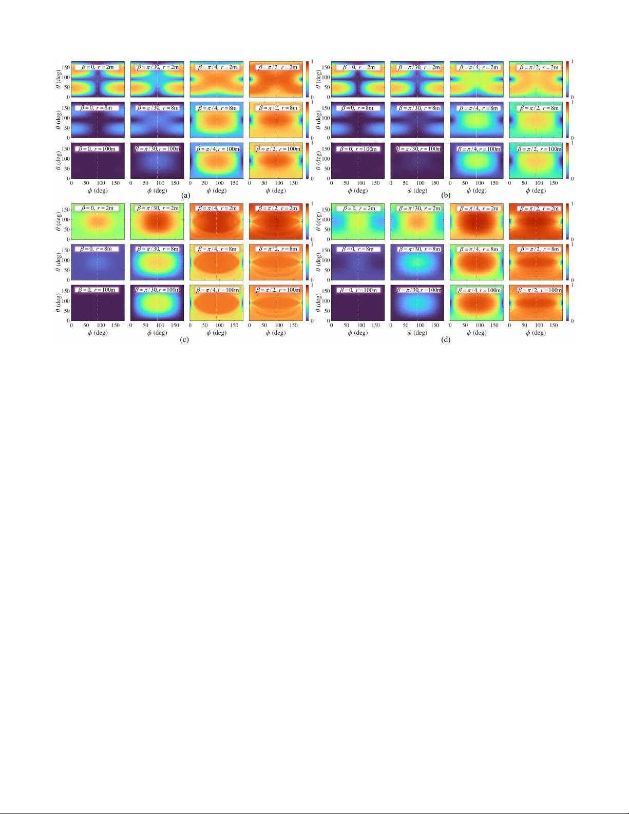
1 Spatial Correlation, Non-Stationarity , and De grees of Freedom of Holographic Curv ature-Reconﬁgurable Apertures Liuxun Xue, Graduate Student Member , IEEE, Shu Sun, Senior Member , IEEE, Ruifeng Gao, Member , IEEE, and Xiaoqian Y i, Senior Member , IEEE Abstract —Low-altitude wireless platforms increasingly require lightweight, conformal, and densely sampled antenna array apertures with high array gain and spatial selectivity . How- ever , when deployed on nonplanar surfaces, curvature alters the array manif old, local visibility , and pr opagation support, potentially in validating spatial-stationarity assumptions. In this paper , we in vestigate a holographic curvatur e-reconﬁgurable aperture (HoloCuRA), modeled as a curvatur e-controllable holo- graphic surface, and develop a visibility-aware spatial charac- terization framework f or its lo w-altitude applications. Specif- ically , the framework jointly quantiﬁes array-domain spatial non-stationarity (SnS), and spatial degrees of freedom (DoF) in line-of-sight, 3GPP non-line-of-sight, and isotropic-scattering propagation envir onments. For SnS, a novel Power -balanced, V isibility-aware Corr elation-Matrix Distance (PoV i-CMD) and a two-stage subarray-screening procedur e are introduced. For DoF , the R ´ enyi-2 effective rank is adopted, and tractable spatial- correlation expressions under isotropic scattering are dev eloped for efﬁcient DoF analysis. Furthermore, a realizable antenna port mode is introduced to connect SnS with DoF . Numerical results re veal that curvatur e and propagation support are the primary determinants of both SnS and DoF in HoloCuRA: array domain SnS determines whether subarray statistics can be treated as locally consistent, whereas DoF limits the global spatial modes. The ﬁndings provide useful guidance for low-altitude antenna- system design. Index T erms —Holographic Curv ature-Reconﬁgurable Aper - ture (HoloCuRA), spatial non-stationarity , visibility region, de- grees of freedom, low-altitude platforms. I . I N T RO D U C T I O N E LECTRICALL Y large, densely sampled antenna ar- ray apertures provide a powerful means to control radiation, focusing, and spatial selecti vity by approaching the continuous-aperture regime. Holographic multiple-input multiple-output (HMIMO) is a representative realization of this paradigm, offering high aperture ef ﬁciency together with substantial geometric ﬂexibility [2], [3]. Nev ertheless, a per- fectly planar aperture is rarely guaranteed in realistic de- A preliminary conference version of part of this work appeared in [1]. The present manuscript substantially e xtends that work with a visibility-aware spatial characterization framework for HoloCuRA, including new spatial non- stationarity analysis, additional propagation scenarios, and new theoretical and numerical results. Liuxun Xue and Shu Sun are with the School of Information and Electronic Engineering, Shanghai Jiao T ong Uni versity , Shanghai 200240, China. (e-mail: liuxun66@sjtu.edu.cn; shusun@sjtu.edu.cn). Ruifeng Gao is with the School of Transportation and Civil Engineering, Nantong Uni versity , Nantong 226019, China (e-mail: grf@ntu.edu.cn). Xiaoqian Y i is with the Flight T est Center , Commercial Aircraft Corporation of China (COMA C), Shanghai 201323, China (e-mail: yixiaoqian@comac.cc). ployments, since bending and warping arise from thin sub- strates, tiled metasurfaces, tolerances, and thermo-mechanical stress, which moti vates curvature reconﬁgurable aperture [4]. Recent advances in ﬂexible intelligent metasurfaces (FIMs), also known as morphable intelligent metasurfaces, provide a natural hardware pathway tow ard curvature-reconﬁgurable apertures [5], [6]. In this work, we speciﬁcally consider con- tinuous, curvature-controllable, reconﬁgurable aperture. Ac- cordingly , such curvature fundamentally modiﬁes the array manifold, local visibility , and propagation support [4]. Conse- quently , planar , far-ﬁeld, and quasi-stationary assumptions can be violated in Holographic Curvature-Reconﬁgurable Aperture (HoloCuRA), making classical conclusions inadequate. It is therefore essential to systematically quantify the resulting spatial propagation characteristics. A. Prior W orks Before analyzing these characteristics in detail, we brieﬂy revie w prior work on spatial non-stationarity (SnS), one of the channel properties most directly affected by aperture curvature. In the literature, SnS is used in two closely related but not identical senses. From a classical stochastic signal- processing perspective, it refers to the violation of wide-sense stationarity (WSS), i.e., the loss of translation in variance in a chosen domain such as time, frequency , or space [7], [8]. By contrast, in propagation and channel-measurement studies, SnS is typically reﬂected by aperture-dependent variations in second-order statistics, such as receiv ed power and cluster visibility [9]. For HoloCuRA, these two vie wpoints naturally coincide, since the electrically large aperture and curvature- induced geometry variations can in validate spatial stationarity ev en within the array domain. Existing SnS studies can be broadly grouped into three cat- egories: (i) measurement-driven characterization across time, frequency , space, and deployment locations, often accompa- nied by SnS-aware channel modeling; (ii) system-lev el SnS- aware design, for extra-large MIMO (XL-MIMO) that ex- plicitly incorporates SnS into transceiv er design and resource management; and (iii) metric and criterion development, for which a uniﬁed and widely accepted standard remains una vail- able. For the ﬁrst category , extensiv e measurement campaigns hav e reported pronounced SnS in XL-MIMO and distributed- MIMO channels [10]–[14]. T o model the underlying mecha- nism that some multipath components (MPCs) are observ able 2 only over portions of the aperture, the concept of visibility region (VR) was introduced and has since been widely adopted in SnS-aware channel models [15]. Building on this insight, research in the second category has primarily explored the new opportunities brought by SnS, especially VR [16]. Rather than enforcing a global stationarity assumption, these studies exploit the fact that different subarrays can observe distinct dominant paths and VRs, which naturally leads to subarray- wise processing and structure-aware channel state information (CSI) acquisition [17]–[19]. The third category of research, which is a main focus of this paper, is to quantify SnS through practical and computable metrics. A representative approach is to measure how the channel’ s spatial structure ev olves by computing distances between correlation matrices estimated at different times/positions, leading to the widely used correlation matrix distance (CMD) [20], [21]. Ho wev er , subsequent analyses of CMD hav e revealed that it may un- derestimate non-stationarity for full-rank cov ariance matrices. Accordingly , eigenv alue-normalized CMD has been proposed to mitigate these limitations [22]. T aken together , these studies show that, although existing SnS metrics are operationally useful, their characterization capability remains incomplete, which motiv ates the metric design and analysis developed in this paper . Another key spatial descriptor is the DoF , which quantiﬁes the number of independent spatial modes supported by a given aperture–propagation conﬁguration and thus determines the effecti ve spatial rank. Although DoF scaling laws are well understood for canonical apertures under far -ﬁeld propagation, including linear , planar , volumetric, and spherical geome- tries [23]–[25], these results do not directly address curv ature- reconﬁgurable holographic apertures. Meanwhile, most exist- ing holographic-aperture analyses still rely on planar abstrac- tions [24]. Such results do not directly extend to conformal apertures or HoloCuRA, where curvature changes local ori- entation, visibility , and the ef fectiv e aperture presented to the propagation ﬁeld, thus requiring geometry-aw are modeling [4], [26], [27]. While conformal-antenna studies hav e extensi vely characterized radiation properties such as beam patterns and efﬁcienc y [4], [28], [29], research on ﬂexible and conformal antennas/arrays has still been largely radiator -oriented, focus- ing on deformation-aware array operation, conformal antenna realization, and curved metasurface-array design rather than channel-lev el spatial characterization [6], [30]–[32]. In con- trast, a systematic characterization of how curvature affects both SnS and DoF in HoloCuRA remains largely open. This gap is fundamental because curvature reshapes HoloCuRA channels at both the local-statistical and global- modal levels. Accordingly , SnS and DoF are adopted here as two complementary descriptors of spatial behavior: SnS and DoF capture two complementary spatial aspects of HoloCuRA channels: SnS reﬂects the local consistency of second-order statistics along the aperture, whereas DoF characterizes the number of globally resolvable spatial modes. Since ignoring SnS can bias subarray modeling and beam management, while ignoring DoF can overestimate spatial parallelism, both must be treated jointly . In HoloCuRA, they are further coupled by curvature through the underlying three-dimensional (3D) Fig. 1. Illustration of a low-altitude HoloCuRA system. propagation geometry . T o e xpose this coupling, we consider the representativ e low-altitude scenario illustrated in Fig. 1. Here, HoloCuRA is deployed on terrestrial or aerial base stations with curved or space-constrained surfaces. W ireless links with unmanned aerial v ehicles (U A Vs), aircraft, and nearby ground or maritime users encounter rapidly varying elev ation and azimuth angles, intermittent blockage, and mixed propagation with dominant line-of-sight (LoS) and local scattering [33]–[36]. Such con- ditions accentuate curvature-induced spatial variations and make low-altitude HoloCuRA a particularly rele vant setting for spatial characterization. B. Our Contrib utions Despite substantial prior work on non-stationary channels and conformal antennas, a rigorous propagation-oriented char- acterization of curv ature-reconﬁgurable holographic apertures remains lacking. Existing SnS studies mainly address time- or user-position-induced variations, with limited attention to array-domain SnS on curv ed dense apertures. Like wise, most av ailable DoF analyses are still rooted in con ventional linear or planar apertures. Meanwhile, related conformal-antenna studies remain largely radiator-oriented, focusing primarily on matching and radiation performance rather than channel- lev el spatial behavior . As a result, a uniﬁed understanding of how curvature reshapes visibility , spatial correlation, array- domain SnS, and effecti ve spatial DoF in HoloCuRA is still missing. T o address this gap, we dev elop a visibility-aware spatial characterization framew ork for HoloCuRA. The main contributions are summarized as follows. • W e establish a uniﬁed spatial characterization frame work for HoloCuRA that jointly analyzes array-domain SnS and DoF across three canonical propagation en viron- ments: LoS, 3GPP NLoS, and isotropic scattering. The framew ork connects local statistical admissibility to full- aperture spatial beha vior under a common curvature- aware setting. • W e propose the Power -balanced and V isibility-aware Correlation Matrix Distance (PoV i-CMD, d PoVi ) for curved apertures. Unlike conv entional CMD-type mea- sures, PoV i-CMD captures both correlation-structure 3 variation and visibility-induced po wer imbalance. Based on this metric, we further de velop a two-stage SnS pro- cedure consisting of local subarray stationarity screening and full-aperture SnS mapping. • W e deriv e tractable spatial-correlation kernels and correlation-matrix expressions for 1D/2D HoloCuRA, with particular emphasis on isotropic scattering, where an efﬁcient analytical DoF characterization is obtained through a closed-form baseline with a bounded one- dimensional correction. This places the DoF analysis on an explicit propagation-correlation foundation and, in the isotropic-scattering case, makes the impact of curvature and propagation support analytically transparent. In this work, the holographic nature of HoloCuRA is essen- tial rather than incidental. Dense holographic sampling pushes the aperture to ward the continuous-aperture re gime, suppresses discretization artifacts, and makes the resulting SnS and DoF behavior primarily geometry- and propagation-dri ven. At the same time, it also provides a practical discrete approximation to the continuous-aperture correlation model and a natural bridge to port limited implementations. C. Or ganization and Notation Or ganization : The remainder of this paper is or ganized as follows. Section II introduces the HoloCuRA geometries. Section III presents the adopted SnS/DoF metrics and the pro- posed PoV i-CMD. Section IV studies LoS spatial characteris- tics, including VR determination, local stationarity screening, and array-domain SnS mapping. Section V considers 3GPP CDL-A channels. Section VI deri ves half-space isotropic- scattering correlation expressions and discusses their SnS/DoF implications. Section VII bridges SnS and DoF via realizable port modes. Section VIII concludes the paper . Notation : Bold lowercase/uppercase letters denote vec- tors/matrices; ( · ) T and ( · ) H denote transpose and conjugate transpose; E {·} denotes expectation; tr( · ) and ∥ · ∥ F denote trace and Frobenius norm; ⊙ denotes the Hadamard product; and a | b means that a divides b . I I . S Y S T E M M O D E L W e consider a BS equipped with HoloCuRA that serves single-antenna users in 3D space. The discrete coordinates be- low represent a uniformly sampled realization of HoloCuRA. This section deﬁnes the one dimension (1D)/ two dimension (2D) aperture geometry and the associated exact and far -ﬁeld array responses used in the subsequent SnS and DoF analysis. Unless otherwise stated, the LoS analysis relies on the exact spherical-wa ve distance, whereas the far-ﬁeld approximation is inv oked later when appropriate for the NLoS and isotropic- scattering settings. A. 1D HoloCuRA Geometry Consider a 1D HoloCuRA with total length L and curv ature radius R , vertically deployed in the YZ-plane as shown in Fig. 2. Let N denote the number of uniformly spaced samples Fig. 2. Geometry and top view of 1D HoloCuRA in 3D space. along the curved aperture, with arc spacing d y z . A single- antenna user is located at u =  r sin θ cos ϕ, r sin θ sin ϕ, r cos θ  , (1) where r denotes the user-to-origin distance, θ is the zenith angle, and ϕ is the azimuth angle. The position of the n -th element is p n =  0 , R cos( β − α n ) − R cos β , R sin( β − α n )  , (2) where β = L 2 R ∈ h 0 , π 2 i , α n = ( n − 1) L ( N − 1) R , n = 1 , . . . , N . (3) The exact user-to-element distance is r u,n = ∥ u − p n ∥ , (4) r u,n = v u u u u u u t  r sin( θ ) cos( ϕ )  2 + h r sin( θ ) sin( ϕ ) − R cos( β − α n ) + R cos( β ) i 2 +  r cos( θ ) − R sin( β − α n )  2 . (5) Accordingly , the exact LoS array response, referenced to the array origin can be expressed as a ( r , θ , ϕ ) = 1 √ N  e − j 2 π λ ( r u, 1 − r ) , . . . , e − j 2 π λ ( r u,N − r )  T , (6) where λ is the carrier w av elength. Under the classical far-ﬁeld condition r ≫ L , a ﬁrst-order e xpansion of (4) yields r u,n ≈ r − ∆ n , (7) with ∆ n = R  sin θ sin ϕ  cos( β − α n ) − cos β  + cos θ sin( β − α n )  . (8) The corresponding far -ﬁeld array manifold is a ( θ , ϕ ) = 1 √ N  e j 2 π λ ∆ 1 , . . . , e j 2 π λ ∆ N  T . (9) B. 2D HoloCuRA Geometry In real-word deployments, planar arrays are more common than linear arrays. Accordingly , 1D HoloCuRA can be ex- tended to 2D HoloCuRA to improve coverage, as illustrated in Fig. 3. Speciﬁcally , the 2D aperture consists of M identical 1D HoloCuRA segments placed at x = md x , m = 1 , . . . , M , with uniform inter-se gment spacing d x . For practical relev ance and uniform aperture sampling, we assume d x = d y z throughout. 4 Fig. 3. Geometry and the ﬁrst-layer slice view of 2D HoloCuRA in 3D space. The ( m, n ) -th element is located at p m,n =  md x , R cos( β − ψ n ) − R cos β , R sin( β − ψ n )  , (10) where ψ n = ( n − 1) L ( N − 1) R ∈ [0 , π ] parameterizes the n -th element on each segment. The symbol ψ n is retained to match Fig. 3; it plays the same geometric role in 2D as α n in the 1D case. The exact user-to-element distance is r ( m,n ) u = ∥ u − p m,n ∥ . (11) r ( m,n ) u = v u u u u t [ r sin( θ ) cos( ϕ ) − md x ] 2 + [ r sin( θ ) sin( ϕ ) − R cos( β − ψ n ) + R cos( β )] 2 + [ r cos( θ ) − R sin( β − ψ n )] 2 . (12) The exact 2D LoS array response, again referenced to the array origin can be written by a 2D ( r , θ , ϕ ) = 1 √ M N  e − j 2 π λ ( r (1 , 1) u − r ) , . . . , e − j 2 π λ ( r ( M,N ) u − r )  T . (13) When the user is in the far ﬁeld relative to both aperture dimensions, i.e., r ≫ max { L, M d x } . A ﬁrst-order e xpansion giv es r ( m,n ) u ≈ r − ∆ m,n , (14) where ∆ m,n = m d x sin( θ ) cos( ϕ ) + R h sin( θ ) sin( ϕ )  cos( β − ψ n ) − cos( β )  + cos( θ ) sin( β − ψ n ) i . (15) The corresponding far -ﬁeld array manifold is a 2D ( θ , ϕ ) = 1 √ M N  e j 2 π λ ∆ 1 , 1 , . . . , e j 2 π λ ∆ M,N  T . (16) The above 1D/2D geometries deﬁne the aperture manifolds used in the subsequent SnS and DoF analysis. In particular , curvature enters through the element coordinates and thereby affects visibility , spatial correlation, and propagation support across the aperture. I I I . S PA T I A L C H A R AC T E R I Z AT I O N M E T R I C S Building on the aperture manifolds in Section II, we char- acterize HoloCuRA through two complementary descriptors: array-domain SnS and effecti ve spatial DoF . SnS is quantiﬁed by the proposed PoV i-CMD, whereas DoF is measured by the R ´ enyi-2 effecti ve rank of the full-aperture correlation matrix. A. P oV i-CMD for VR-A war e SnS Classical CMD measures the similarity between correlation structures, b ut it normalizes away absolute po wer and therefore cannot reﬂect VR-induced power inconsistency across subar- rays. For HoloCuRA, howe ver , visibility interruption alters not only the correlation structure but also the power supported by each visible subspace. Motiv ated by this, we introduce a Power-Balanced and V isibility-A ware CMD, which jointly captures structural decorrelation and visibility-induced power mismatch. Consider either a 1D HoloCuRA with N ant = N elements or a 2D HoloCuRA with N ant = M N elements. Let h = [ h 1 , . . . , h N ant ] T ∈ C N ant × 1 denote the full-array channel, and partition the aperture into K equal-size subarrays { S k } K k =1 , where S k = { i k, 1 , . . . , i k,N sub } and N sub = | S k | . The corre- sponding subarray channel is h k = [ h i k, 1 , . . . , h i k,N sub ] T . For a scenario-dependent visible set V p ⊆ { 1 , . . . , N ant } , deﬁne the binary mask v k = [ v k, 1 , . . . , v k,N sub ] T with v k,j = 1 if i k,j ∈ V p and v k,j = 0 otherwise. The VR-gated (visible) channel is then h vr k = h k ⊙ v k (17) which yields the visible spatial correlations R vr kk = E { h vr k ( h vr k ) H } , R vr kℓ = E { h vr k ( h vr ℓ ) H } . (18) where R vr kk is the auto-correlation matrix of the VR channel vector h vr k , and R vr kℓ is the corresponding cross-correlation matrix between h vr k and h vr ℓ , k and ℓ index two (possibly dif- ferent) channel vectors (e.g., the k -th and ℓ -th subarrays/links). Then, the deﬁned PoV i-CMD with a power exponent q ≥ 1 can be formulated as γ kℓ = tr( R vr kk R vr ℓℓ ) ∥ R vr kk ∥ F ∥ R vr ℓℓ ∥ F , (19) α kℓ = ∥ R vr kk ∥ F ∥ R vr ℓℓ ∥ F , (20) f q ( α ) = 2 α q + α − q = sec h  q | ln α |  , q ≥ 1 , (21) and d kℓ PoVi ( q ) = 1 − γ kℓ f q ( α kℓ ) ∈ [0 , 1] . (22) Here, γ kℓ measures correlation-structure coherence, α kℓ captures the visible-power ratio, and f q ( α kℓ ) penalizes log- power mismatch, attaining 1 at α kℓ = 1 and vanishing as α kℓ → 0 or α kℓ → ∞ . Unless otherwise stated, d kℓ PoVi denotes d kℓ PoVi ( q ) for a ﬁxed design choice of q . B. Effective Spatial DoF T o quantify the global modal support of HoloCuRA, we adopt the R ´ enyi-2 effecti ve rank of the full-aperture spatial correlation matrix R = E { hh H } . Let { λ i } denote the eigen- values of R , and deﬁne p i = λ i / P j λ j . The R ´ enyi-2 entropy is H 2 = − log  P i p 2 i  , which gi ves the ef fecti ve rank [37] exp( H 2 ) = 1 P i p 2 i = ( P i λ i ) 2 P i λ 2 i =  tr( R )  2 ∥ R ∥ 2 F . (23) Since (23) is in variant to any positiv e scaling of R , it mea- sures eigen value spread rather than absolute power and thus 5 quantiﬁes the effecti ve number of supported spatial modes. Unless otherwise stated, DoF is computed from the full R without VR gating, since the objective here is to characterize the physical modal ceiling of the aperture–propagation pair; the associated visibility-limited realizability loss is treated later in Section VII. W e also report the normalized DoF n DoF = N DoF N ant . (24) In summary , d PoVi is stationarity-oriented, since it mea- sures cross-subarray statistical consistency under VR gating, whereas N DoF is mode-oriented, since it summarizes the total number of spatial modes supported by the full aperture. T ogether, they provide a compact and physically grounded characterization frame work for the subsequent LoS, NLoS, and isotropic-scattering analysis. I V . L O S S P A T I A L C H A R AC T E R I Z AT I ON : V I S I B I L I T Y , S N S , A N D D O F W ith the metrics in Section III in place, we turn to the LoS case, where the impact of curvature is most directly gov erned by aperture geometry , spherical-wav e propagation, and self- occlusion. The analysis proceeds in two stages. W e ﬁrst deri ve an explicit visible-region (VR) criterion and use it to determine admissible subarray partitions through a local stationarity test. W e then characterize the resulting array-domain SnS over the full aperture and complement it with a DoF view under LoS- dominant sparse propagation. A. Geometric V isible-Region Determination 1) VR Criterion for 1D HoloCuRA: For 1D HoloCuRA in the y – z plane, LoS visibility is gov erned by conv ex self- occlusion. Let the n -th element be located at p n and let the effecti ve center of curv ature be C = (0 , − R cos β , 0) . The outward unit normal at element n is ˆ n n = p n − C R =  0 , cos γ n , sin γ n  , γ n = β − α n . (25) Let the user position be u . By the tangent-plane test, element n is visible if ( u − p n ) · ˆ n n ≥ 0 ⇔ ( u − C ) · ˆ n n ≥ R . (26) Substituting (25) into (26) yields r g n ( θ , ϕ ) ≥ R  1 − cos β cos γ n  , (27) where g n ( θ , ϕ ) = sin θ sin ϕ cos γ n + cos θ sin γ n , (28) Γ n ( r , β , γ n ) = R r  1 − cos β cos γ n  . (29) Hence, the VR condition is g n ( θ , ϕ ) ≥ Γ n ( r , β , γ n ) . (30) Under free-space LoS propagation, h LoS n = p G t G r λ 4 π r un e − j 2 π λ r un , r un = ∥ u − p n ∥ , where G t and G r are the transmit and recei ve antenna gains and are set to unity . For the adopted 1D deployment, the binary VR mask v LoS n ∈ { 0 , 1 } is activ ated at ϕ = π / 2 through (30), whereas for ϕ  = π / 2 we set v LoS n = 1 . The VR-aware LoS channel is then h LoS - VR = v LoS ⊙ h LoS . (31) 2) Extension to 2D HoloCuRA: For 2D HoloCuRA, the same geometric criterion applies row-wise along the curved dimension, but the visibility test is ev aluated over the full azimuth range. In implementation, we compute the mask along the arc direction and replicate it across the x -dimension. The resulting mask directly gates the LoS channel, yielding the VR-aware 2D response without further geometric modiﬁca- tion. 3) Geometric Implications of the VR Criterion: The cri- terion in (30) highlights two vital properties. First, there is no single distance r that guarantees full visibility for all look directions, because visibility depends jointly on ( θ , ϕ ) , r , and β . Second, e ven in the far-ﬁeld limit ( r → ∞ ), full visibility is not automatic; the outward half-space condition still requires g n ( θ , ϕ ) ≥ 0 . In the planar limit β → 0 , (30) reduces to the familiar half-space test. B. Local SnS Criterion and Admissible Subarray Design 1) Local Stationarity Criterion: In LoS, VR-induced non- stationarity ﬁrst appears locally within each subarray . W e therefore determine admissible subarray partitions before e val- uating full-aperture SnS. For 1D HoloCuRA, the aperture is divided into K contiguous subarrays of equal size N sub = N K , K | N . (32) For 2D HoloCuRA, a grid partition is speciﬁed by ( g z , g x ) such that K = g z g x , g z | N , g x | M , (33) with tile size tileZ = N g z , tileX = M g x , N sub = tileZ · tileX . (34) For a ﬁxed K , we consider all feasible factor pairs ( g z , g x ) satisfying the abov e di visibility constraints. Thus, larger g z produces thinner strips along z (smaller tileZ ), while larger g x produces narro wer tiles along x (smaller tileX ). Each tile (subarray) contains N sub = tileZ · tileX elements. 1 Let Ω = ( θ , ϕ ) denote a sampled half-space direction, and let h i (Ω; β , r ) be the VR-aware LoS channel at element i , with in visible elements set to zero. Deﬁne the element-wise po wer a i (Ω) ≜ | h i (Ω) | 2 . (35) For subarray S k , let µ k (Ω) and v k (Ω) be the mean and variance of { a i (Ω) : i ∈ S k } , and deﬁne the relati ve variance η k (Ω) ≜ v k (Ω) µ k (Ω) 2 , µ k (Ω) > 0 . (36) Direction Ω is declared locally passing if η k (Ω) ≤ 1 /e . 2 Over all sampled directions { Ω t } N Ω t =1 , deﬁne the activ e set V k ≜ { t : µ k (Ω t ) > 0 } (37) 1 For example, with K = 64 and N z = N x = 128 , “Z-cut” corresponds to Grid 64 × 1 (tiles of size 2 × 128 ), whereas “X-cut” corresponds to Grid 1 × 64 (tiles of size 128 × 2 ). Other grids (e.g., 2 × 32 , 8 × 8 ) cut both dimensions and yield tileZ × tileX tiles. 2 The 1 /e threshold is commonly used in channel modeling [36] and provides a practical boundary between locally ﬂat and visibly non-uniform power proﬁles. 6 Fig. 4. Local stable subarray fraction as a function of β (rad) for 1D HoloCuRA with N = 128 , L = 0 . 32 m , and r = 2 . 0 m : (a) ϕ = 90 ◦ (VR activ e) and (b) the ϕ  = 90 ◦ region, both plotted versus the number of subarrays K ∈ { 2 , 4 , 8 , 16 , 32 , 64 } . V alues closer to 1 indicate that a larger fraction of subarrays remains stable for the corresponding curvature/partition setting. and the pass probability P k ≜ 1 | V k | X t ∈ V k 1  η k (Ω t ) ≤ 1 e  . (38) Subarray k is declared locally stationary if P k ≥ 0 . 7 . 3 This two-le vel test ﬁrst checks local ﬂatness for each direction and then retains only partitions that remain stable over a strong majority of visible directions. 2) P artition Candidates and Evaluation Setup: Low- altitude links in the millimeter -wav e/sub-THz regime are often LoS-dominant or NLoS with directionally sparse scattering. The small wav elength also makes a ﬁxed physical aperture electrically large ( D /λ ), which pushes the radiating near-ﬁeld (Fresnel region) to meter-/tens-of-meters link ranges, thereby making array-domain SnS easier to excite and observe. In addition, the selected ranges should be consistent with classical aperture distance bounds. Building on this, we ev aluate the local criterion at f c = 30 GHz with ﬁxed aperture length L = 0 . 32 m and curvature β ∈ (0 , π / 2] . Following standard aperture-distance criteria, we use the chord length as the effecti ve aperture size, whose extrema are D max = L, D min = 2 L π ≈ 0 . 2037 m . (39) The reactiv e near-ﬁeld bound and Rayleigh distance [38] are R react ( D ) ≈ 0 . 62 r D 3 λ , R Rayleigh ( D ) = 2 D 2 λ . (40) T aking conservati ve e xtrema o ver β giv es R react , max = R react ( D max ) ≈ 1 . 12 m , (41) R Rayleigh , min = R Rayleigh ( D min ) ≈ 8 . 30 m . (42) Accordingly , we use r ∈ { 2 , 8 , 100 } m as representa- tiv e near-ﬁeld, upper-near-ﬁeld, and far -ﬁeld operating points, whereas 100 m is well beyond the Rayleigh distance for any curvature and serves as a far -ﬁeld baseline representativ e of typical low-altitude links. 3 The threshold 0 . 7 is adopted as a strong-majority rule: it requires that the local ﬂatness criterion holds for most ( ≥ 70% ) of the visible directions, while a small ( ≤ 30% ) fraction of outliers is tolerated. Fig. 5. Local stable subarray fraction as a function of β (rad) for 2D HoloCuRA local-SnS at r = 2 . 0 m for (a) K = 16 and (b) K = 32 , comparing different partition schemes (X-cut, Z-cut, and 2D grid partitions with the indicated grid sizes). V alues closer to 1 indicate that a larger fraction of subarrays remains stable for the corresponding curvature/partition setting. 3) Admissible P artition Selection: Fig. 4 and Fig. 5 show that, in 1D HoloCuRA, local SnS is dominated by VR- induced self-occlusion, whereas curvature alone causes only mild de gradation aw ay from the edge-on azimuth. In 2D HoloCuRA, increasing K enlarges the admissible region be- cause smaller subarrays span shorter VR gradients and weaker near-ﬁeld po wer variation. The contrast between X-cut and Z- cut reveals that the dominant visibility variation is along the curved z -dimension. Here, X-cut partitions the aperture along x , yielding tiles that are narrow in x but long in z , whereas Z- cut partitions along z , yielding tiles that are thin in z but wide in x . Consequently , X-cut is more likely to mix rows with markedly different visibility states within the same subarray , producing larger intra-subarray power variation, whereas Z- cut better conforms to the underlying visibility structure and is therefore more locally stationary . Guided by the above observations, we retain only those partition scales whose subarray footprint remains locally ad- missible under the LoS visibility v ariation, leading to K ULA ∈ { 8 , 16 } for 1D HoloCuRA and K URA ∈ { 16 , 32 } for 2D HoloCuRA. For 2D HoloCuRA, we further retain both Z- cut and representative 2D grids, because they probe two physically distinct ways in which curvature-induced visibility and propagation v ariation are distributed ov er the aperture: slicing along the dominant z -directed visibility gradient and compact two-dimensional tiling over the aperture surface. Concretely , for K = 16 we compare Grid 16 × 1 with Grid 4 × 4 , and for K = 32 we compare Grid 32 × 1 with Grid 8 × 4 . The resulting partitions contain roughly 512 – 1024 elements per subarray , so that each subarray remains at a moderate and physically meaningful aperture scale rather than an arbitrarily ﬁne discretization. Hence, subarray partitioning should not be interpreted as a free post-processing choice, nor does it create SnS; instead, it deﬁnes the aperture-domain observ ation scale at which the underlying geometry- and propagation-induced non-stationarity is represented. C. Array-Domain SnS under LoS After selecting admissible partitions, we ev aluate full- aperture SnS by aggregating the pairwise PoV i-CMD deﬁned in Section III. Local and array-domain SnS play different roles: the former determines whether a candidate partition 7 Fig. 6. Heatmaps of the half-space-averaged array-domain metric d PoVi (color scale) for 1D HoloCuRA. For each direction ( θ, ϕ ) , the shown value is d PoVi av eraged over all K ( K − 1) / 2 subarray pairs using a Z-cut partition. Columns correspond to the array curvature β ∈ { 0 , π / 30 , π / 4 , π / 2 } , and rows correspond to the link distance r ∈ { 2 , 8 , 100 } m . (a) K = 8 and (b) K = 16 . The vertical dashed line marks ϕ = 90 ◦ . Results are shown for d el = λ/ 4 ; the corresponding d el = λ/ 2 patterns are visually almost indistinguishable, and additional checks with d el = λ/ 16 lead to the same qualitativ e trends. remains locally admissible, whereas the latter quantiﬁes the statistical disparity among subarrays ov er the full aperture. For each sampled direction ( θ, ϕ ) , let d kℓ PoVi denote the VR-aw are pairwise discrepancy between subarrays k and ℓ , as deﬁned in (19)–(22). W e then deﬁne the mean array-domain SnS lev el as d mean PoVi ( θ , ϕ ) = 2 K ( K − 1) X k<ℓ d kℓ PoVi ( θ , ϕ ) , (43) and map d mean PoVi ( θ , ϕ ) over the sampled half-space. W e empha- size that the retained K values are not introduced to create SnS, b ut to probe the same geometry- and propagation-induced non-stationarity at dif ferent admissible observation scales. 1) Near-to-F ar-F ield SnS of 1D HoloCuRA: Fig. 6 shows d mean PoVi ( θ , ϕ ) for multiple ranges and curv atures. As β in- creases, the high-SnS region broadens, while the dominant ridge remains centered near θ ≈ 90 ◦ . For mild curvature, SnS decreases with r , which is consistent with the weakening of spherical-wav e amplitude and phase gradients as the link mov es tow ard the far ﬁeld. For larger β , the dependence on r becomes weaker , because the mismatch is then dominated by curvature-induced boresight di ver gence together with per- sistent VR-driven po wer imbalance. The SnS heatmaps obtained with d el = λ/ 2 and d el = λ/ 4 are visually almost indistinguishable, so only the d el = λ/ 4 results are shown here for brevity . Additional checks with d el = λ/ 16 yield the same qualitative patterns, which indicates Fig. 7. SnS versus elev ation angle θ for 1D HoloCuRA at azimuth ϕ = π / 2 and range r = 2 m . (a)–(c) correspond to array curvature β = 0 , β = π/ 4 , and β = π / 2 , respecti vely . T wo SnS measures are compared: the con ventional CMD metric and the proposed d PoVi . For β ∈ { π / 4 , π / 2 } , results with and without VR modeling are both shown; for β = 0 , all elements are visible and only the VR-aware curves are plotted. The shown results use d el = λ/ 4 ; the corresponding d el = λ/ 2 and d el = λ/ 16 curves are visually almost indistinguishable. that the dominant SnS behavior is gov erned by the underlying aperture geometry and propagation rather than by the sampling grid itself. In this sense, dense holographic sampling does not create SnS, but suppresses discretization artifacts and makes its continuous-aperture origin more faithfully observable. T o sharpen the angular interpretation, Fig. 7 plots θ -cuts at ϕ = π / 2 . As β increases, the low-SnS trough contracts and the proﬁle e volv es into a high plateau with ripples, consistent with alternating inter-subarray alignment and misalignment compounded by VR on/off transitions. Unlike CMD, which is in v ariant to scalar power scaling, d PoVi remains sensitiv e to VR-induced po wer imbalance through its po wer-balancing term and therefore gives a stronger and more range-robust indication of LoS SnS. 2) Near-to-F ar-F ield SnS of 2D HoloCuRA: Fig. 8 reports the array-domain SnS heatmaps of 2D HoloCuRA under the selected admissible partition schemes. For the Z-cut partition at short range ( r = 2 m ), a distinctiv e four-lobe pattern appears. This structure is caused by the spherical-wav e phase variation along the x -dimension, which contains both a linear tilt term and a quadratic curv ature term, and whose interplay produces symmetric correlation valle ys across subarrays. As r increases, the quadratic contribution decays on the order of 1 /r , so the lobes are gradually smoothed and the SnS contours become more circular . For the representativ e 2D grids, the partition resolves both the z -directed visibility variation and the x -directed phase variation over the aperture. Under stronger curv ature, the vis- ibility boundary intersects more tiles, which creates partially visible subarrays and richer angular textures than in the Z-cut 8 Fig. 8. Heatmaps of the half-space-averaged array-domain metric d PoVi (color scale) for 2D HoloCuRA as a function of direction ( θ, ϕ ) (in degrees). (a) and (c) show the case K = 16 , using a Z-cut partition (Grid 16 × 1 , tile 8 × 128 ) and a 2D grid partition (Grid 4 × 4 , tile 32 × 32 ), respecti vely . (b) and (d) show the case K = 32 , using a Z-cut partition (Grid 32 × 1 , tile 4 × 128 ) and a 2D grid partition (Grid 8 × 4 , tile ≈ 16 × 32 or 32 × 16 ), respectively . The v ertical dashed line marks ϕ = 90 ◦ . Results are shown for d el = λ/ 4 ; the corresponding d el = λ/ 2 patterns are visually almost indistinguishable, and additional checks with d el = λ/ 16 lead to the same qualitative trends. case. Across both 1D and 2D HoloCuRA, the array-domain SnS increases with curvature, whereas increasing K mainly changes the observation scale: smaller subarrays are naturally more similar , but the same geometry- and propagation-induced trends remain. As in the 1D case, the heatmaps obtained with d el = λ/ 2 and d el = λ/ 4 are visually almost indistinguishable, so only the d el = λ/ 4 results are shown here. Additional checks with d el = λ/ 16 again lead to the same qualitati ve patterns. This shows that, for a ﬁxed physical aperture, reducing d el mainly reﬁnes the sampling of the same continuous ﬁeld rather than reshaping the underlying SnS pattern. By contrast, increasing K changes the subarray footprint at which that ﬁeld is observed. Hence, the weakening of the av eraged SnS lev el at larger K should be interpreted as a scale effect rather than as the disappearance of the underlying physical non-stationarity . This distinction is precisely where holographic sampling is useful: once the aperture is densely sampled, the observed SnS reﬂects the aperture-domain geometry and propagation more than the sampling grid itself. Despite these common trends, 1D and 2D HoloCuRA re- main fundamentally dif ferent. The 2D aperture preserves gen- uine azimuth–elev ation discrimination and therefore supports a richer spatial organization of SnS than its 1D counterpart. D. Spatial DoF under LoS-Dominant Sparse Pr opagation 1) LoS Reference and CDL-D Baseline: A pure single-ray LoS channel is rank-one and therefore serves as a geometric reference rather than a realistic modal baseline. T o obtain a realistic, typical low-altitude, and reproducible LoS-type baseline beyond a single-ray specular model, and to av oid the scenario dependence and limited transferability of geometry- speciﬁc ray tracing, we adopt the 3GPP clustered delay line (CDL) model [39]. Here we use the standardized 3GPP CDL-D channel model, which includes a dominant specular component together with a limited number of clusters and ﬁnite angular spreads. This provides a sparse-support refer- ence that remains consistent with lo w-altitude LoS-dominant propagation. 2) Eigen-Spectrum and DoF Comparison: As sho wn in Fig. 9, under the CDL-D model both 1D and 2D HoloCuRA exhibit eigen-spectra that are strongly concentrated at lo w orders and decay rapidly thereafter , which indicates that the effecti ve DoF is activ ated only over a limited set of domi- nant spatial modes under LoS-dominant sparse propagation. Relativ e to 1D HoloCuRA, the 2D aperture sustains a longer tail and a later spectral knee, because the additional aperture dimension preserves extra spatial discrimination under the same sparse angular support. By contrast, the single-ray LoS reference remains essentially rank-one and therefore serves mainly as a geometric lo wer-comple xity baseline. The impact of curvature β is secondary compared with the ov erall lo w-rank structure, b ut it is not negligible. Its effect appears primarily in the high-order tail, where cur - vature perturbs the array manifold through changes in local aperture orientation and projected propagation support. This 9 Fig. 9. Sorted eigen value spectra of the HMIMO spatial correlation matrix under a LoS link and the 3GPP CDL-D channel model for HoloCuRA. (a) 1D HoloCuRA with half-wavelength inter-element spacing d = λ/ 2 ( N ant = 64 ). (b) 2D HoloCuRA with d = λ/ 2 ( N ant = 64 2 ). (c) 1D HoloCuRA with quarter-wa velength spacing d = λ/ 4 ( N ant = 128 ). (d) 2D HoloCuRA with d = λ/ 4 ( N ant = 128 2 ). Eigen values are ordered in decreasing magnitude. V ertical dashed lines indicate the HMIMO spatial DoF limits: 2 L/λ for the 1D array and min( πL 2 /λ 2 , L CDL − D ) for the 2D array . Here L CDL − D denotes the effecti ve DoF upper bound imposed by the 3GPP CDL-D multipath channel model. perturbation is more visible for 2D HoloCuRA, since the extra aperture dimension allows curvature-induced changes to be distributed ov er a richer set of weak modes. In 1D HoloCuRA, howe ver , the array remains intrinsically one-dimensional, so under CDL-D’ s LoS-dominant e xcitation the higher-order tail need not e volv e monotonically with β ; instead, curv ature mainly reshapes a small number of weakly excited modes without altering the overall low-order concentration. Comparing the d el = λ/ 2 cases in Fig. 9(a)–(b) with the d el = λ/ 4 cases in Fig. 9(c)–(d) further sho ws that denser holographic sampling reﬁnes the spectral representation but does not materially shift the dominant spectral knee or the effecti ve DoF . For 1D HoloCuRA, the λ/ 2 sampling exhibits an almost hard truncation after the knee, whereas λ/ 4 mainly rev eals additional near-zero modes be yond the effecti ve cutof f without creating new signiﬁcant ones. For 2D HoloCuRA, the main dif ference is again spectral resolution: the denser sampling provides more eigen v alue samples over the same DoF re gion and yields a clearer depiction of the roll-of f near the cutoff, while the cutoff location itself is essentially preserved. T aken together, these results show that in LoS-dominant sparse propagation the effecti ve DoF is governed primarily by aperture dimensionality and propagation support, whereas curvature mainly acts as a secondary perturbation on the eigen v alue tail. In this sense, holographic sampling does not increase the physical DoF of a ﬁxed aperture, b ut improves the ﬁdelity with which the underlying eigen-spectrum is resolved and interpreted. E. Joint LoS Insights on SnS and DoF Under LoS, the half-space heatmaps of d PoVi show where different subarrays still exhibit similar statistics and where they begin to dif fer over ( θ, ϕ ) , r , and β . In this sense, the proposed SnS framew ork does more than assign a scalar non-stationarity lev el: by combining VR-aware subarray partitioning with a local-to-global screening procedure, it turns curv ature-induced spatial heterogeneity into an explicit aperture-domain charac- terization that can be resolved ov er direction and range. The LoS results further sho w that array-domain SnS is not a single-mechanism effect. Rather , it is jointly produced by spherical-wav e propagation, curv ature-dependent, and VR- induced visibility interruption. These mechanisms act on dif- ferent b ut coupled scales: spherical-wave gradients dominate in the radiating near ﬁeld, curvature reshapes the aperture response through local orientation changes, and VR introduces abrupt power imbalance through self-occlusion. Their com- bined action makes the per -element and per-subarray responses strongly location dependent, especially at short range. V iewed together with the DoF results, this leads to a clear design implication for HoloCuRA. One is that local SnS screening is indispensable for selecting admissible subarray sizes and orientations under self-occlusion and near-ﬁeld ef- fects, thereby enabling stable subarray lev el processing and calibration. The other is that the pronounced eigenv alue con- centration under CDL-D shows diminishing DoF returns in di- rectionally sparse en vironments. Therefore, under low-altitude LoS conditions, array-domain SnS directly indicates whether curvature- and VR-induced aperture v ariation is strong enough to support subarray-wise operation: large SnS fav ors parti- tioned use of HoloCuRA, whereas small SnS suggests that the aperture should be used more effecti vely as a single coherent surface. V . N L O S S P A T I A L C H A R AC T E R I Z AT I O N U N D E R N O N - I S OT R O P I C S C A T T E R I N G T o extend the LoS geometry-dominated analysis to a statis- tically grounded NLoS setting, we retain the d PoVi framew ork so that SnS is quantiﬁed on a common scale across propagation en vironments. In NLoS, howe ver , non-stationarity is no longer gov erned by explicit self-occlusion alone, but by non-isotropic angular support and curvature-dependent spatial correlation. This section therefore examines how curvature reshapes the angular support, how array domain SnS differs from spatial WSS, and how these effects relate to the effecti ve DoF under CDL-A. A. Non-Isotr opic Scattering Model and SnS Indicators 1) Curvatur e-Dependent Angular Support: Under NLoS non-isotropic scattering, the spatial correlation is computed from the discrete three-dimensional angular power spectrum speciﬁed by the CDL model. Unlike the LoS case, where backside scattering is neglected and the effecti ve support reduces to a β -independent front half-space, NLoS propagation admits non-negligible backside contrib utions, which produce a β -dependent coverage extension. Speciﬁcally , bending rotates 10 Fig. 10. Z-cut maps of SnS for 1D HoloCuRA in the 3GPP CDL-A (NLoS) channel. The mean SnS is shown in (a)–(b) and the SnS variance in (c)–(d), as functions of the subarray separation s and curvature β (rad). Panels (a),(c) correspond to K = 8 , whereas (b),(d) correspond to K = 16 (the grid/tile settings used for each case are indicated above each subplot). the local surface normal of each element ov er [ − β , β ] , en- larging the union of forward-visible directions. The additional backside support is thus conﬁned to the two elev ation caps θ ∈ [0 , β ] ∪ [ π − β , π ] , (44) while spanning the full azimuth range ϕ ∈ [0 , 2 π ] . 2) SnS Mean and V ariance V ersus Subarray Separation: A second distinction from LoS is that, under NLoS, the channel is characterized by multi-cluster angular support with distinct AoA/AoD statistics under the standard far -ﬁeld as- sumption [39]. In this setting, pointwise directional compari- son is less informati ve than a separation-based array-domain summary . W e therefore deﬁne two SnS indicators over the subarray separation s = | k − ℓ | : the mean discrepanc y ¯ d ( s ; β ) = 1 K − s K − s X k =1 d PoVi ( k , k + s ; β ) , (45) and the corresponding same-separation v ariance V ar s ( β ) = V ar k =1 ,...,K − s [ d PoVi ( k , k + s ; β )] . (46) If the array-domain statistics were spatially WSS along the aperture, they would be in v ariant to index translation, which implies V ar s ( β ) = 0 for e very s . Hence, ¯ d ( s ; β ) measures the ov erall SnS strength, whereas V ar s ( β ) quantiﬁes the departure from spatial WSS. B. CDL-A Baseline and Evaluation Setup T o obtain a standardized and reproducible NLoS base- line, we adopt CDL-A from 3GPP TR 38.901 [39]. CDL-A features relativ ely narro w three-dimensional angular spreads, e.g., c ASA = 11 ◦ and c ZSA = 3 ◦ , which is consistent with directionally sparse lo w-altitude NLoS links dominated by a limited number of strong clusters. The same admissible partition scales selected in the LoS section are retained here so that the comparison across propagation en vironments is performed under a common subarray architecture. C. SnS Behavior Under CDL-A 1) 1D HoloCuRA: For 1D HoloCuRA, Fig. 10 sho ws that ¯ d ( s ; β ) exhibits visible ripples over ( s, β ) , reﬂecting the discrete angular support of CDL-A: with only a ﬁnite number of dominant clusters and rays, small geometry-induced phase reweightings can produce constructiv e and destuctive changes in the averaged SnS. Increasing K reduces the overall SnS lev el because smaller subarrays are naturally more similar . Fig. 11. Comparison of Z-cut and grid-based ev aluations of SnS for HoloCuRA under the 3GPP CDL-A channel. Heatmaps of the mean SnS are shown in (a)–(d), and those of the SnS variance in (e)–(h), versus the subarray separation s and curv ature β (rad). Results for K = 16 are given in (a),(b),(e),(f), and results for K = 32 are given in (c),(d),(g),(h). For each K , the Z-cut maps are shown in (a),(c),(e),(g), while the corresponding grid- based maps are shown in (b),(d),(f),(h). Grid/tile conﬁgurations are indicated above each subplot; colorbars report the mean SnS (top row) and variance (bottom ro w). Meanwhile, V ar s ( β ) remains nearly negligible, indicating that in this 1D setting the discrepancy is governed primarily by the subarray separation s rather than by the absolute subarray location. 2) 2D HoloCuRA: For 2D HoloCuRA, Fig. 11 shows that ¯ d ( s ; β ) generally increases with both curvature β and separa- tion s . Under Z-cut, the mean-SnS surface is mildly wa vy yet remains approximately monotone, consistent with a dominant variation direction along the aperture. Under grid partitioning, the same s can mix subarray pairs from different physical directions. Because curvature inﬂuences different directions unequally , the resulting heatmap exhibits regular stripe-like patterns. Since curvature does not af fect all directions equally , pairs aligned with the more sensitiv e direction, where element orientation and cluster visibility vary more strongly , exhibit larger SnS, whereas pairs aligned mainly with less sensitive directions exhibit smaller SnS. Such stripes are not artifacts, but a physically meaningful reﬂection of the directional nature of the 2D curved aperture. Despite these texture dif ferences, the main trends are con- sistent across CDL-A and across both 1D and 2D HoloCuRA: (i) SnS remains weak as β → 0 , corresponding to nearly linear or planar apertures; (ii) SnS decreases as K increases, because the same non-stationarity is observed at a ﬁner subarray scale; and (iii) SnS increases with both curvature and subarray separation. Moreover , the lo w le vel of V ar s ( β ) indicates that CDL-A, although non-isotropic, still concentrates most of its variation into a limited number of dominant directions rather than producing a strongly position-dependent random result ov er the aperture. D. Spatial DoF Under CDL-A Fig. 12 shows the eigen value spectra of the spatial corre- lation matrices for 1D and 2D HoloCuRA under CDL-A. In all cases, the spectra roll off well before the physical-aperture DoF bound, which indicates that the effecti ve DoF is primarily 11 Fig. 12. Sorted eigen value spectra of the spatial correlation matrix for HoloCuRA under the 3GPP CDL-A NLoS channel. (a),(c) 1D HoloCuRA with N ant = 64 and N ant = 128 , respectively; (b),(d) 2D HoloCuRA with N ant = 64 2 and N ant = 128 2 , respecti vely . Eigenv alues are ordered in decreasing magnitude and plotted versus the eigen value index on a logarithmic scale. The vertical dashed lines indicate the spatial DoF limits: 2 L/λ for the ULA and min( π L 2 /λ 2 , L CDL − A ray ) for the URA, where L CDL − A ray denotes the DoF ceiling imposed by the ﬁnite number of paths in the CDL-A model. scattering-limited in this NLoS scenario. As β increases, the truncation point tends to move to ward higher orders, although not strictly monotonically , reﬂecting the interaction between curvature-induced manifold perturbation and sparse angular support. The comparison between d el = λ/ 2 and d el = λ/ 4 follows the same pattern as in the LoS case: denser holographic sampling reﬁnes the spectral representation but does not materially shift the dominant knee or the effecti ve DoF . For 1D HoloCuRA, the ﬁner sampling mainly reveals additional weak modes beyond the cutoff; for 2D HoloCuRA, it provides a denser sampling of the same roll-off region. Thus, under CDL-A the effecti ve DoF remains controlled primarily by the av ailable scattering support and aperture dimensionality , while curv ature acts mainly as a secondary perturbation of the eigen v alue tail. E. Joint NLoS Insights on SnS and DoF T aken together , the NLoS results show that curvature af- fects HoloCuRA through two coupled mechanisms. First, by reshaping the angular support and the corresponding spatial correlation, it modiﬁes the array-domain SnS and can make a global WSS approximation ev en under a standardized CDL baseline. Second, through the same support reshaping, it per - turbs the eigen-spectrum and slightly redistributes the usable spatial modes, although the dominant DoF bottleneck remains the limited number of excited scattering directions. Therefore, under NLoS non-isotropic scattering, the spatial behavior of HoloCuRA cannot be inferred from aperture size or sampling density alone. SnS still depends on ho w curv ature interacts with the dominant scattering directions and how the aperture is partitioned, whereas DoF remains bounded primarily by the a vailable propagation support. This conﬁrms that curv ature, subarray geometry , and scattering structure must be considered jointly when characterizing HoloCuRA under realistic NLoS conditions. V I . I S OT R O P I C S P A T I A L C H A R AC T E R I Z A T I O N : C L O S E D - F O R M C O R R E L A T I O N , S N S , A N D D O F Consistent with the holographic viewpoint of this paper, we model HoloCuRA as a quasi-continuous electromagnetic aperture and deriv e its spatial correlation under half-space isotropic scattering. Unlike the LoS and NLoS cases, where spatial heterogeneity is shaped by visibility interruption or non-isotropic angular support, isotropic scattering provides a reference in which the role of curvature becomes analytically transparent. This section therefore serves as the continuous- aperture baseline of the paper: it yields closed-form correlation expressions for 1D and 2D HoloCuRA, clariﬁes the ef fect of curvature-induced cov erage extension, and provides a weak- SnS reference against which the stronger non-stationarity observed under LoS and NLoS can be interpreted. A. Continuous-Apertur e Isotr opic Corr elation Model W e begin from the spatial correlation matrix R = E  a ( θ , φ ) a H ( θ , φ )  , (47) whose entries are angular integrals weighted by a scattering function S ( θ , φ ) . If S ( θ , φ ) is normalized over an integration domain D , i.e., Z Z D S ( θ , φ ) d Ω = 1 , (48) then the diagonal entries satisfy [ R ] m,m = 1 , and R is a correlation-coefﬁcient matrix. Throughout this section we adopt half-space isotropic scattering ov er D 0 = [0 , π ] × [0 , π ] [23], S ( θ , φ ) = sin θ 2 π , ( θ , φ ) ∈ D 0 , (49) and use the normalized sinc function sinc( x ) = sin( π x ) / ( π x ) . 1) 1D HoloCuRA: Baseline Corr elation and Cover age Ex- tension: Under D 0 and the dominant zeroth-order approxima- tion, the baseline correlation of 1D HoloCuRA depends only on the central-angle separation α n − α m and admits the closed form [1] [ R 0 ] m,n ≈ sinc  4 R λ sin  α n − α m 2  . (50) Bending may additionally expose part of the backside azimuth support at e xtreme elev ations. W e model this cov erage extension through Ω ext ( β ) ≜  ( θ , φ ) : θ ∈ [0 , β ] ∪ [ π − β , π ] , φ ∈ [ π , 2 π ]  , (51) while keeping S ( θ , φ ) unchanged. The total correlation can then be decomposed as R m,n ( β ) = R 0 ,m,n + R extra ,m,n ( β ) , (52) 12 where the extension term reduces to the bounded one- dimensional correction R extra ,m,n ( β ) ≈ Z 1 cos β cos  bu cos c  × J 0  b p 1 − u 2 sin c  du, (53) with u = cos θ and b = 4 π R λ sin  α n − α m 2  , (54) c = β − α m + α n 2 . (55) Because the angular domain is enlar ged without re- normalizing S ( θ , φ ) , the diagonal power increases to R m,m ( β ) = Z Z D 0 ∪ Ω ext ( β ) sin θ 2 π d Ω = 2 − cos β . (56) Accordingly , the normalized correlation-coefﬁcient matrix is ˜ R m,n ( β ) = R m,n ( β ) 2 − cos β . (57) 2) 2D HoloCuRA: Baseline Corr elation and Cover age Ex- tension: For 2D HoloCuRA, the same half-space isotropic model yields the baseline correlation between elements ( m, n ) and ( m ′ , n ′ ) as [1] R (0) ( m,n ) , ( m ′ ,n ′ ) ≈ sinc  2 λ p D 2 + E 2  , (58) where the geometric quantities D and E are      D = r ( m − m ′ ) 2 d 2 + 4 R 2 sin 2  ψ n − ψ n ′ 2  sin 2  β − ψ n + ψ n ′ 2  , E = 2 R cos  β − ψ n + ψ n ′ 2  sin  ψ n − ψ n ′ 2  . (59) Using the same cov erage-extension region (51), the total correlation becomes R ( m,n ) , ( m ′ ,n ′ ) ( β ) ≈ R (0) ( m,n ) , ( m ′ ,n ′ ) + R extra , ( m,n ) , ( m ′ ,n ′ ) ( β ) , (60) where the extension term again reduces to a bounded one- dimensional integral, R extra , ( m,n ) , ( m ′ ,n ′ ) ( β ) ≈ Z 1 cos β cos( k 0 E u ) · J 0  k 0 D p 1 − u 2  du. (61) with k 0 = 2 π /λ and u = cos θ . As in the 1D case, the diagonal equals the total collected average po wer over D 0 ∪ Ω ext ( β ) and is therefore giv en by 2 − cos β . The normalized correlation- coefﬁcient matrix is ˜ R ( m,n ) , ( m ′ ,n ′ ) ( β ) = R ( m,n ) , ( m ′ ,n ′ ) ( β ) 2 − cos β . (62) T aken together, the 1D and 2D results show that under isotropic scattering the HoloCuRA correlation reduces to a sinc-type baseline plus a bounded one-dimensional correction. This is precisely where the holographic viewpoint is most useful: once the aperture is treated as densely sampled, the underlying continuous-aperture correlation kernel becomes both analytically tractable and physically interpretable. B. Corr elation-Coefﬁcient Matrices for 1D and 2D HoloCuRA The normalized matrices ˜ R iso ( β ) in (57) and (62) provide a uniﬁed second-order description of isotropic HoloCuRA. For any prescribed subarray partition with index sets {I k } K k =1 , the corresponding subarray correlation blocks are obtained directly as ˜ R iso ( β )[ I k , I ℓ ] , so that the SnS metrics based on d PoVi can be e valuated de- terministically , without additional angular sampling or Monte- Carlo averaging. This direct block extraction is important because it connects the continuous-aperture correlation model to the same subarray-level framework used in the LoS and NLoS sections. C. SnS Under Isotr opic Scattering Under isotropic scattering, angular av eraging smooths out direction-speciﬁc irre gularities and yields a near -stationary second-order reference. In the planar limit ( β = 0 ), the result- ing matrix reduces to a T oeplitz structure for 1D HoloCuRA and to a block-T oeplitz-with-T oeplitz-blocks structure for 2D HoloCuRA. Consequently , for any equal-size contiguous or grid partition, equal-separation subarray pairs share the same or nearly the same second-order statistics, which implies a near-zero same-separation SnS v ariance and a mean SnS that depends primarily on the subarray displacement rather than on the absolute aperture location. For β > 0 , bending introduces only a bounded coverage- extension correction and a smooth diagonal scaling by 2 − cos β . Hence, curv ature perturbs the isotropic correlation kernel only mildly and preserves near translation in variance ov er the aperture. In this sense, isotropic scattering provides a weak-SnS baseline: the observed non-stationarity remains small, and stronger SnS in the LoS and NLoS sections should therefore be interpreted as arising from visibility interrup- tion or non-isotropic angular support rather than from the HoloCuRA alone. D. Spatial DoF Under Isotropic Scattering Building on the same cov erage-extended isotropic corre- lation model, we next examine the effecti ve DoF through the eigen value spectrum. As β increases, the visible angular domain expands and the set of supported inter -element phase differences becomes richer . Consequently , spatial correlation weakens and spectral energy spreads from a few dominant modes to higher orders, which appears as a rightward shift of the spectral knee in Fig. 13(a)–(b). Because the matrices hav e already been diagonal-normalized, this shift reﬂects a redistribution of modal energy rather than an ov erall power increase. The detailed tail behavior is then set by aperture dimension- ality . For 1D HoloCuRA, the additional support introduced by curv ature remains relati vely well aligned with the baseline one-dimensional manifold, so the ener gy redistribution is con- centrated mainly among the leading eigenmodes and the high- order tail remains comparativ ely weak. For 2D HoloCuRA, by contrast, the e xtra aperture dimension allo ws the additional 13 Fig. 13. Sorted eigen value spectra of the spatial correlation matrix for HoloCuRA under isotropic scattering. (a),(c) 1D HoloCuRA with N ant = 64 and N ant = 128 , respecti vely; (b),(d) 2D HoloCuRA with N ant = 64 2 and N ant = 128 2 , respectively . Eigenv alues are ordered in decreasing magnitude and plotted v ersus the (dimensionless) eigen v alue index on a logarithmic scale. Marker curves correspond to the curvature parameter β (see legends). V ertical dashed lines indicate the spatial DoF limits, 2 L/λ for the ULA and π L 2 /λ 2 for the URA; insets in (c) and (d) zoom into the cutof f region. support to populate eigen-directions that are less aligned with the baseline subspace, which produces a more pronounced high-order tail. The comparison between λ/ 2 and λ/ 4 further clariﬁes the role of holographic sampling. In 1D HoloCuRA, the λ/ 2 case is effecti vely close to critical sampling relati ve to the aperture DoF , so the spectrum appears as a near-ﬂat plateau followed by a sharp drop. The λ/ 4 case does not increase the physical DoF , but resolves the post-cutoff transition much more clearly , as highlighted by the inset in Fig. 13(c). The same effect is ev en more visible in 2D HoloCuRA, where the denser sampling produces a much richer spectral trace around the cutoff in Fig. 13(d). Across all three en vironments, this role of dense sampling is most transparent under isotropic scattering, because the channel e xcites the full set of aperture- supported modes and the continuous-aperture interpretation is least obscured by directional sparsity . E. Joint Isotr opic Insights on Corr elation, SnS, and DoF This isotropic case plays a distinct role in the paper . It is not merely a third propagation scenario, but the continuous- aperture reference against which the stronger and more struc- tured non-stationarity of the LoS and NLoS cases should be understood. The closed-form correlation kernels show ex- plicitly how curvature enters through geometry and coverage extension, while the SnS results show that this geometric effect alone produces only weak array-domain heterogeneity under isotropic av eraging. At the same time, the DoF results clarify the main contribution of the holographic viewpoint. Dense sampling does not create ne w physical modes for a ﬁxed aperture; instead, it exposes the underlying continuous- aperture eigenspectrum more faithfully and makes curvature- dependent redistribution of modal energy analytically visible. In this sense, isotropic scattering provides the cleanest link among correlation, SnS, DoF , and holographic sampling, and therefore serv es as the theoretical anchor of the full HoloCuRA characterization developed in this paper . V I I . R E A L I Z A B L E A N T E N NA P O RT M O D E S : B R I D G I N G S N S A N D P H Y S I C A L D O F A. Motivation and Deﬁnition Having characterized array-domain SnS via d PoVi heatmaps and physical spatial DoF via eigen-spectra in the preceding sections, we now connect these two views at the implementa- tion le vel for port-limited HoloCuRA. W e focus on the LoS case, where low-altitude links are often LoS-dominant and SnS is primarily geometry dri ven by spherical-wav e gradients, curvature projection, and VR gating, making the resulting port mode budget physically interpretable and transferable. While physical DoF speciﬁes the modal ceiling of the full aperture, practical HoloCuRA implementations are realized through a ﬁnite number of subarray ports. This motiv ates the follo wing question: under LoS, how many subarray ports are effecti vely non-redundant and can therefore act as distinct aperture modes? The proposed PoV i-CMD provides a bounded Fig. 14. Realizable port mode versus β for HoloCuRA under lo w-altitude half-space averaging. A near-ﬁeld LoS channel is considered with f c = 30 GHz and ﬁxed user range r = 2 m . (a) 1D HoloCuRA ( L = 0 . 32 m , N = 128 ): R eﬀ ( r, β ) (right axis) and R eﬀ /K (left axis) for K ∈ { 8 , 16 } . (b) 2D HoloCuRA ( 0 . 32 m × 0 . 32 m , 128 × 128 ): R eﬀ ( r, β ) for K ∈ { 16 , 32 } under representati ve z -cut and 2D grid port arrangements. (c) R eﬀ /K for the same arrangements as in (b). For comparison, the 2D arrangements are as follows. For K = 16 : Grid 16 × 1 (tile 8 × 128 elements) versus Grid 4 × 4 (tile 32 × 32 ). For K = 32 : Grid 32 × 1 (tile 4 × 128 ) versus Grid 8 × 4 (tile ≈ 16 × 32 ). pairwise dissimilarity that jointly captures VR gating, po wer 14 imbalance, and correlation-shape mismatch across subarrays. W e therefore use it to construct an inter-port similarity matrix and a realizable port mode dimension. For a HoloCuRA implemented with K subarray ports, deﬁne at each Ω = ( θ , ϕ ) [ S (Ω)] kℓ ≜ s kℓ (Ω) =    1 , k = ℓ, q 1 − d kℓ PoVi (Ω) , k  = ℓ, (63) where d kℓ PoVi (Ω) is deﬁned in (22), with γ kℓ (Ω) and α kℓ (Ω) giv en in (19)–(20), and f q ( · ) in (21). Larger PoV i-CMD values imply weaker inter-port similarity and hence lower port redundancy . Here, S (Ω) is used only as a bounded symmetric summary of inter-port similarity under LoS; it is not an element-lev el cov ariance matrix, and the construction belo w does not require a PSD or kernel interpretation. W e then deﬁne a realizable port mode dimension in the same trace-ratio form used for physical DoF: r eﬀ (Ω) =  tr S (Ω)  2 ∥ S (Ω) ∥ 2 F =  tr S (Ω)  2 tr  S 2 (Ω)  . (64) Since tr S (Ω) = K , r eﬀ (Ω) = K 2 K + 2 P k<ℓ s 2 kℓ (Ω) = K 2 K + 2 P k<ℓ  1 − d kℓ PoVi (Ω)  . (65) Moreov er , since 0 ≤ s kℓ (Ω) ≤ 1 for all k  = ℓ , we hav e K ≤ tr  S 2 (Ω)  = K + 2 X k<ℓ s 2 kℓ (Ω) ≤ K 2 , (66) which together with (64) yields 1 ≤ r eﬀ (Ω) ≤ K . (67) Hence, r eﬀ (Ω) → 1 when most ports remain highly similar, whereas r eﬀ (Ω) → K when SnS strongly differentiates the ports. Thus, r eﬀ (Ω) quantiﬁes the number of approximately non-redundant port modes av ailable at Ω . B. A ver aging and Relation to Physical DoF A scenario-le vel b udget is obtained by av eraging over the operating domain Ω dom . For lo w-altitude LoS operation, Ω dom is taken as the relev ant half-space: R eﬀ ( r , β ) = E Ω ∈ Ω dom  r eﬀ (Ω)  . (68) Unless otherwise stated, the expectation in (68) is taken with respect to a uniform angular measure over the lo w-altitude half-space. The quantity R eﬀ ( r , β ) is not a new physical DoF . Rather , DoF phys remains the modal ceiling of the full aperture, whereas R eﬀ describes ho w many approximately independent port modes can be realized under a given subarray-port ar- rangement. This moti vates the practical bound N port - mo des ( r , β ) ≲ min  R eﬀ ( r , β ) , DoF phys , N RF  . (69) where N RF denotes the number of RF chains. C. Impact of Curvature and P ort Arrangement for the Low- Altitude W e ev aluate R eﬀ ( r , β ) over the low-altitude half-space using the same setup as in Sec. IV , with subarray sizes chosen to satisfy the local-stationarity condition. The local-stationarity condition is used only to deﬁne an admissible port granularity , whereas R eﬀ summarizes the residual inter -port similarity across such admissible ports. For 1D HoloCuRA, Fig. 14(a) sho ws that both R eﬀ and R eﬀ /K increase monotonically with β , indicating that cur- vature reduces inter-port similarity and enlarges the realizable port mode b udget. Ho wev er , increasing the number of subarray ports does not necessarily increase R eﬀ : relative to K = 8 , the K = 16 case yields smaller R eﬀ and lower R eﬀ /K , rev ealing substantial redundancy under excessiv e subdivision in 1D. A similar redundancy effect appears for 2D HoloCuRA under z -cut arrangements in Fig. 14(b)–(c): R eﬀ grows with β but decreases when K increases from 16 to 32 because the additional ports remain highly similar . By contrast, the 2D grid arrangements markedly improv e both R eﬀ and R eﬀ /K , indicating that localized 2D port organization better captures incident-ﬁeld diversity and reduces similarity accumulation. Collectiv ely , these trends directly yield low-altitude design guidance. When β is small or the chosen arrangement giv es a small R eﬀ , subarray merging is preferred for robust coherent focusing. Con versely , when β is sufﬁciently large and the arrangement achie ves a larger R eﬀ , separated ports can support more agile beamforming, multiplexing, or nulling, subject to (69). Hence, R eﬀ ( r , β ) serves as an implementation-level budget for port-limited HoloCuRA, while DoF phys remains the physical modal ceiling. V I I I . C O N C L U S I O N In this paper , we dev eloped a spatial characterization frame- work for lo w-altitude HoloCuRA by jointly analyzing array- domain SnS and spatial DoF under LoS, 3GPP NLoS, and isotropic scattering propagation en vironments. For SnS, we proposed PoV i-CMD and established a two-stage local-to- global procedure, in which VR-aware local admissibility ﬁrst determines physically meaningful subarray partitions and full- aperture SnS is then characterized on that basis. The results show that LoS SnS is driven jointly by spherical-wa ve gradi- ents, curv ature-dependent projection, and self-occlusion prop- agation en vironments, whereas in NLoS curvature reshapes non-isotropic angular support. For spatial DoF , we adopted the R ´ enyi-2 effecti ve rank and clariﬁed the role of holographic sampling through a uniﬁed propagation-correlation view . In particular , the isotropic case serves as a theoretical anchor: 1D and 2D HoloCuRAs admit tractable closed-form correlation expressions, which show that the effecti ve spatial DoF is governed mainly by aper- ture dimensionality and propagation support, while curv ature acts primarily through support reshaping and tail-lev el eigen- spectrum perturbation. Dense holographic sampling does not create ne w physical modes for a ﬁxed aperture size, but suppresses discretization artifacts and rev eals the underlying continuous-aperture correlation and eigenspectrum more faith- fully . Finally , by mapping PoV i-CMD into a port-similarity 15 matrix, we connected SnS to a realizable antenna port mode budget, thereby bridging spatial characterization and port- limited low-altitude holographic aperture design. A P P E N D I X A D E R I V A T I O N S F O R 1 D H O L O C U R A C O R R E L A T I O N W I T H C OV E R AG E E X T E N S I O N A. Covera ge extension term and 1D inte gral form W ith Ω ext ( β ) in (51), R extra ,m,n ( β ) = Z Ω ext ( β ) sin θ 2 π e j ∆ m,n ( θ,φ ) dφ dθ. (70) For a given θ , deﬁne I ( π , 2 π ) φ ( θ ) = Z 2 π π e j ∆ m,n ( θ,φ ) dφ. (71) Let z ≜ b sin θ sin c (with b, c in (54)). Then I ( π , 2 π ) φ ( θ ) = e j b cos θ cos c Z 2 π π e − j z sin φ dφ. (72) Exact f orm. W ith φ ′ = φ − π and sin( φ ′ + π ) = − sin φ ′ [40], Z 2 π π e − j z sin φ dφ = Z π 0 e j z sin φ ′ dφ ′ = Z π 0 cos( z sin φ ′ ) dφ ′ + j Z π 0 sin( z sin φ ′ ) dφ ′ = π J 0 ( z ) + j Ξ( z ) . (73) where Ξ( z ) ≜ R π 0 sin( z sin t ) dt . Even-part (zeroth-order) approximation. Retaining only the real (even) part of (73), Z 2 π π e − j z sin φ dφ ≈ π J 0 ( z ) . (74) Thus, I ( π , 2 π ) φ ( θ ) ≈ π e j b cos θ cos c J 0  b sin θ sin c  . (75) Substituting (75) into (70) yields R (0) extra ,m,n ( β ) = 1 2  Z β 0 + Z π π − β  sin θ e j b cos θ cos c J 0  b sin θ sin c  dθ . (76) Using the cap symmetry θ 7→ π − θ giv es R (0) extra ,m,n ( β ) = Z β 0 sin θ cos  b cos θ cos c  J 0  b sin θ sin c  dθ . (77) Finally , with u = cos θ , and b, c in (54) R (0) extra ,m,n ( β ) = Z 1 cos β cos  bu cos c  J 0  b p 1 − u 2 sin c  du. (78) A P P E N D I X B D E R I V A T I O N S F O R 2 D H O L O C U R A C O R R E L A T I O N W I T H C OV E R AG E E X T E N S I O N A. Covera ge extension term and 1D inte gral form The phase dif ference between ( m, n ) and ( m ′ , n ′ ) is [1] ∆ m,n − ∆ m ′ ,n ′ = A ( θ ) cos φ + B ( θ ) sin φ + C ( θ ) . (79) Deﬁne t nn ′ ≜ β − ψ n + ψ n ′ 2 , s nn ′ ≜ sin  ψ n − ψ n ′ 2  . (80) Then A ( θ ) = ( m − m ′ ) d x sin θ, B ( θ ) = − 2 R sin θ sin( t nn ′ ) s nn ′ , C ( θ ) = 2 R cos θ cos( t nn ′ ) s nn ′ . (81) Let k 0 = 2 π /λ and deﬁne Φ( θ , φ ) ≜ A ( θ ) cos φ + B ( θ ) sin φ + C ( θ ) . (82) W ith Ω ext ( β ) in (51), R extra ( β ) = Z Ω ext ( β ) sin θ 2 π e − j k 0 Φ( θ,φ ) dφ dθ. (83) For a given θ , deﬁne I ( π , 2 π ) φ ( θ ) ≜ Z 2 π π e − j k 0 Φ( θ,φ ) dφ. (84) Let ρ ( θ ) ≜ p A ( θ ) 2 + B ( θ ) 2 and choose δ ( θ ) such that cos δ ( θ ) = A ( θ ) ρ ( θ ) , sin δ ( θ ) = B ( θ ) ρ ( θ ) . (85) Then A cos φ + B sin φ = ρ cos( φ − δ ) and I ( π , 2 π ) φ ( θ ) = e − j k 0 C ( θ ) Z 2 π π e − j k 0 ρ ( θ ) cos( φ − δ ( θ )) dφ φ ′ = φ − π = e − j k 0 C ( θ ) Z π 0 e + j k 0 ρ ( θ ) cos ( φ ′ − δ ( θ ) ) dφ ′ . (86) Even/odd decomposition and zer oth-order approximation. For bre vity , let x ≜ k 0 ρ ( θ ) and δ ≜ δ ( θ ) . Using Euler’ s identity , Z π 0 e j x cos ( φ ′ − δ ) dφ ′ = Z π 0 cos  x cos( φ ′ − δ )  dφ ′ + j Z π 0 sin  x cos( φ ′ − δ )  dφ ′ . (87) The even (real) part admits the standard Bessel representation R π 0 cos( x cos t ) dt = π J 0 ( x ) . Retaining only this ev en part yields Z π 0 e j x cos ( φ ′ − δ ) dφ ′ ≈ π J 0 ( x ) . (88) Thus, I ( π , 2 π ) φ ( θ ) ≈ π e − j k 0 C ( θ ) J 0  k 0 ρ ( θ )  . (89) From (81), ρ ( θ ) = D sin θ and C ( θ ) = E cos θ hold with D = q ( m − m ′ ) 2 d 2 x + 4 R 2 s 2 nn ′ sin 2 ( t nn ′ ) , E = 2 R s nn ′ cos( t nn ′ ) . (90) Substituting (89) into (83) yields R (0) extra ( β ) = 1 2  Z β 0 + Z π π − β  sin θ e − j k 0 E cos θ J 0  k 0 D sin θ  dθ = Z β 0 sin θ cos  k 0 E cos θ  J 0  k 0 D sin θ  dθ u =cos θ = Z 1 cos β cos( k 0 E u ) J 0  k 0 D p 1 − u 2  du. (91) 16 R E F E R E N C E S [1] L. Xue, S. Sun, and H. Y an, “Spatial correlation and degrees of freedom in arched HMIMO arrays: A closed-form analysis, ” in Proc. IEEE 101st V eh. T echnol. Conf. (VTC-Spring) , Jun. 2025, pp. 1–6. [2] C. Huang, S. Hu, G. C. Alexandropoulos, A. Zappone, C. Y uen, R. Zhang, M. Di Renzo, and M. Debbah, “Holographic MIMO surfaces for 6G wireless networks: Opportunities, challenges, and trends, ” IEEE W ir eless Commun. , vol. 27, no. 5, pp. 118–125, Oct. 2020. [3] R. Deng, B. Di, H. Zhang, D. Niyato, Z. Han, H. V . Poor , and L. Song, “Reconﬁgurable holographic surfaces for future wireless communica- tions, ” IEEE W ir eless Commun. , vol. 28, no. 6, pp. 126–131, Jan. 2022. [4] L. Josefsson and P . Persson, Conformal Array Antenna Theory and Design . Hoboken, NJ, USA: Wile y–IEEE Press, 2006. [5] J. An, C. Y uen, M. Di Renzo, M. Debbah, H. V . Poor , and L. Hanzo, “Flexible intelligent metasurfaces for downlink multiuser MISO com- munications, ” IEEE Tr ans. W ireless Commun. , vol. 24, no. 4, pp. 2940– 2955, Apr . 2025. [6] I. Y oo and D. R. Smith, “Design of conformal array of rectangular wav eguide-fed metasurfaces, ” IEEE T rans. Antennas Pr opag. , v ol. 70, no. 7, pp. 6060–6065, Jul. 2022. [7] G. Matz, “On non-WSSUS wireless fading channels, ” IEEE T rans. W ir eless Commun. , vol. 4, no. 5, pp. 2465–2478, Sep. 2005. [8] X. Gao, F . Tufv esson, and O. Edfors, “Massiv e MIMO channels— measurements and models, ” in Pr oc. Asilomar Conf. Signals, Syst. Comput. , No v . 2013, pp. 280–284. [9] E. de Carvalho, A. Ali, A. Amiri, M. Angjelichinoski, and R. W . Heath, “Non-stationarities in extra-lar ge-scale massive MIMO, ” IEEE W ir eless Commun. , v ol. 27, no. 4, pp. 74–80, 2020. [10] Z. Y uan, J. Zhang, Y . Ji, G. F . Pedersen, and W . Fan, “Spatial non- stationary near-ﬁeld channel modeling and validation for massiv e MIMO systems, ” IEEE T rans. Antennas Pr opag. , v ol. 71, no. 1, pp. 921–933, Jan. 2023. [11] J. Bian, C.-X. W ang, X. Gao, X. Y ou, and M. Zhang, “ A general 3D non-stationary wireless channel model for 5G and beyond, ” IEEE T rans. W ir eless Commun. , vol. 20, no. 5, pp. 3211–3224, May 2021. [12] H. Xu, P . T ang, J. Zhang, H. Xing, L. Tian, and Q. W ang, “ An empirical study on near-ﬁeld, spatial non-stationarity , and beam misalignment characteristics of THz XL-MIMO channels at 132 GHz, ” in Pr oc. IEEE Int. Conf. Commun. W orkshops (ICC W orkshops) , Jun. 2024, pp. 744– 749. [13] X. Gao, O. Edfors, F . Tufv esson, and E. G. Larsson, “Massive MIMO in real propagation environments: Do all antennas contribute equally?” IEEE T rans. Commun. , vol. 63, no. 11, pp. 3917–3928, Nov . 2015. [14] Y . Xu, M. Sandra, X. Cai, S. W illhammar , and F . T ufvesson, “Charac- terization of non-wide-sense stationarity for distributed massive MIMO channels, ” in Pr oc. 19th Eur . Conf. Antennas Propa g. (EuCAP) , 2025, pp. 1–5. [15] J. Flordelis, X. Li, O. Edfors, and F . Tufv esson, “Massiv e MIMO extensions to the COST 2100 channel model: Modeling and validation, ” IEEE Tr ans. W ir eless Commun. , vol. 19, no. 1, pp. 380–394, Jan. 2020. [16] X. Li, S. Zhou, E. Bj ¨ ornson, and J. W ang, “Capacity analysis for spatially non-wide-sense stationary uplink massiv e MIMO systems, ” IEEE Tr ans. Wir eless Commun. , vol. 14, no. 12, pp. 7044–7056, Dec. 2015. [17] L. Pang, W . Han, Y . Zhang, H. Jin, Y . Chen, A. W ang, and J. Li, “Time- frequency-space joint extrapolation for 6G near-ﬁeld non-stationary massiv e MIMO channels, ” IEEE Commun. Lett. , vol. 29, no. 8, pp. 1953–1957, Aug. 2025. [18] Y . Chen and L. Dai, “Non-stationary channel estimation for extremely large-scale MIMO, ” IEEE T rans. W ir eless Commun. , vol. 23, no. 7, pp. 7683–7697, Jul. 2024. [19] X. W ang, H. Chen, R. Jiang, T . Liu, J. Zhao, and Y . Xu, “Near-ﬁeld wideband non-stationary channel estimation for XL-MIMO based on frequency-dependent visibility region, ” IEEE T rans. Cogn. Commun. Netw . , vol. 12, pp. 3987–4001, 2026. [20] M. Herdin, N. Czink, H. Ozcelik, and E. Bonek, “Correlation matrix distance, a meaningful measure for evaluation of non-stationary MIMO channels, ” in Pr oc. IEEE 61st V eh. T echnol. Conf. (VTC-Spring) , vol. 1, 2005, pp. 136–140. [21] E. P . Simon, P . Laly , V . Picquet, and D. P . Gaillot, “Exploring MIMO correlation matrix distance for cell-free V2I channel characterization, ” IEEE Antennas W ir eless Pr opag . Lett. , pp. 1–5, Oct. 2025. [22] O. Aldayel, M. Bengtsson, and S. A. Alshebeili, “Ev aluation of MIMO channel non-stationarity , ” in Proc. 21st Eur . Signal Process. Conf. (EUSIPCO) , Sep. 2013, pp. 1–5. [23] S. Sun and M. T ao, “Characteristics of channel eigen v alues and mutual coupling effects for holographic reconﬁgurable intelligent surfaces, ” Sensors , vol. 22, no. 14, p. 5297, Jul. 2022. [24] A. Pizzo, T . L. Marzetta, and L. Sanguinetti, “Degrees of freedom of holographic MIMO channels, ” in Proc. IEEE 21st Int. W orkshop Signal Pr ocess. Adv . Wir eless Commun. (SP A WC) , May 2020, pp. 1–5. [25] A. S. Y . Poon, R. W . Brodersen, and D. N. C. Tse, “Degrees of freedom in multiple-antenna channels: A signal space approach, ” IEEE T rans. Inf . Theory , v ol. 51, no. 2, pp. 523–536, Feb . 2005. [26] T . G. Pelham, G. Hilton, E. Mellios, and R. Le wis, “Predicting conformal aperture gain from 3D aperture and platform models, ” IEEE Antennas W ir eless Propag . Lett. , vol. 16, pp. 700–703, Sep. 2017. [27] I. Y oo and D. R. Smith, “Design of conformal array of rectangular wav eguide-fed metasurfaces, ” IEEE T rans. Antennas Pr opag. , v ol. 70, no. 7, pp. 6060–6065, Jan. 2022. [28] R. J. Allard, D. H. W erner , and P . L. W erner , “Radiation pattern synthesis for arrays of conformal antennas mounted on arbitrarily-shaped three- dimensional platforms using genetic algorithms, ” IEEE Tr ans. Antennas Pr opag. , vol. 51, no. 5, pp. 1054–1062, May 2003. [29] Y . J. Cheng, H. Xu, D. Ma, J. Wu, L. W ang, and Y . Fan, “Millimeter- wav e shaped-beam substrate integrated conformal array antenna, ” IEEE T rans. Antennas Pr opag . , v ol. 61, no. 9, pp. 4558–4566, Sep. 2013. [30] M.-C. T ang, Y . Duan, Z. W u, and M. Li, “Flexible, conformal, endﬁre radiating, electrically small antennas on a conducting cylinder with a small radius, ” IEEE T rans. Antennas Pr opag . , vol. 68, no. 5, pp. 3496– 3503, Jan. 2020. [31] B. D. Braaten, S. Roy , S. Nariyal, M. Al Aziz, N. F . Chamberlain, I. Irfanullah, M. T . Reich, and D. E. Anagnostou, “ A self-adapting ﬂexible (SELFLEX) antenna array for changing conformal surface applications, ” IEEE T rans. Antennas Pr opag . , vol. 61, no. 2, pp. 655– 665, Feb . 2013. [32] A. S. M. Sayem, R. B. V . B. Simorangkir, K. P . Esselle, and R. M. Hashmi, “Development of rob ust transparent conformal antennas based on conductive mesh-polymer composite for unobtrusive wearable appli- cations, ” IEEE T rans. Antennas Propag . , vol. 67, no. 12, pp. 7216–7224, Dec. 2019. [33] W . Khawaja, I. Guvenc, D. W . Matolak, U.-C. Fiebig, and N. Schneck- enbur ger , “ A surv ey of air-to-ground propagation channel modeling for unmanned aerial vehicles, ” IEEE Commun. Surveys T uts. , vol. 21, no. 3, pp. 2361–2391, May 2019. [34] N. H. Motlagh, T . T aleb, and O. Arouk, “Low-altitude unmanned aerial vehicles-based internet of things services: Comprehensi ve surve y and future perspectives, ” IEEE Internet Things J . , v ol. 3, no. 6, pp. 899– 922, Sep. 2016. [35] Z. Xu, T . Zheng, and L. Dai, “LLM-empowered near-ﬁeld communica- tions for low-altitude economy , ” IEEE T rans. Commun. , vol. 73, no. 11, pp. 11 186–11 196, No v . 2025. [36] S. Sun, Y . Guo, M. T ao, W . Feng, J. Chen, R. Gao, Y . Li, J. W ang, and T . S. Rappaport, “Modeling and analysis of land-to-ship maritime wireless channels at 5.8 GHz, ” IEEE T rans. W ir eless Commun. , vol. 25, pp. 10 051–10 065, 2026. [37] A. R ´ enyi, “On measures of entropy and information, ” in Proc. 4th Berkele y Symp. Math. Statist. Pr obab ., V ol. 1: Contributions to the Theory of Statistics . Berkeley , CA, USA: Univ . California Press, 1961, pp. 547–561. [38] S. Sun, R. Li, C. Han, X. Liu, L. Xue, and M. T ao, “How to differentiate between near ﬁeld and far ﬁeld: Revisiting the Rayleigh distance, ” IEEE Commun. Mag . , v ol. 63, no. 1, pp. 22–28, Jan. 2025. [39] 3rd Generation Partnership Project (3GPP), “Study on channel model for frequencies from 0.5 to 100 GHz, ” 3GPP , T ech. Rep. TR 38.901, v19.1.0, Rel. 19, Oct. 2025. [40] F . Bowman, Intr oduction to Bessel Functions . North Chelmsford, U.K.: Courier Corporation, 2012.

Spatial Correlation, Non-Stationarity, and Degrees of Freedom of Holographic Curvature-Reconfigurable Apertures

Original Paper

Comments & Academic Discussion

Leave a Comment

Original Paper

Related Papers

Comments & Academic Discussion

Leave a Comment