Identification of NMF by choosing maximum-volume basis vectors
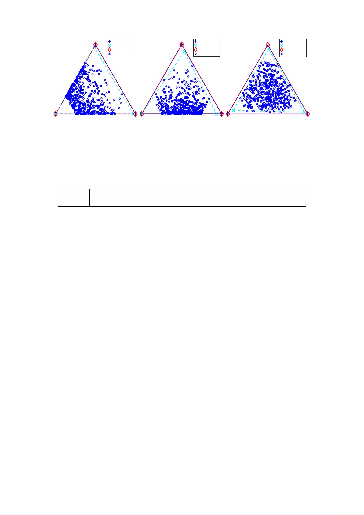
In nonnegative matrix factorization (NMF), minimum-volume-constrained NMF is a widely used framework for identifying the solution of NMF by making basis vectors as similar as possible. This typically induces sparsity in the coefficient matrix, with e…
Authors: Qianqian Qi, Zhongming Chen, Peter G. M. van der Heijden
Identification of NMF by choosing maximum-volume basis vectors Qianqian Qi Hangzhou Dianzi University , China q.qi@hdu.edu.cn Zhongming Chen Hangzhou Dianzi University , China zmchen@hdu.edu.cn Peter G. M. van der Heijden Utrecht University , the Netherlands and University of Southampton, UK p.g.m.vanderheijden@uu.nl Abstract In nonnegative matrix factorization (NMF), minimum-vol ume-constrained NMF is a widely used framework for identifying the solution of NMF by making basis vec- tors as similar as possible. This typically induces sparsity in the coefficient matrix, with each row containing zer o entries. Consequently , minimum-volume-constrained NMF may fail for highly mixed data, where such sparsity does not hold. Moreover , the estimated basis vectors in minimum-volume-constrained NMF may be difficult to interpret as they may be mixtur es of the ground truth basis vectors. T o address these limitations, in this paper we propose a new NMF framework, called maximum- volume-constrained NMF , which makes the basis vectors as distinct as possible. W e further establish an identifiability theorem for maximum-volume-constrained NMF and provide an algorithm to estimate it. Experimental results demonstrate the ef fec- tiveness of the proposed method. Keywords: Nonnegative matrix factorization, maximum-volume basis vectors, unique- ness, algorithm 1 Introduction Nonnegative matrix factorization (NMF) has been a workhorse method used in many ar- eas, such as blind hyperspectral unmixing, blind sound separation, image processing, text mining, and signal processing [ 1 , 2 , 3 ]. It aims to approximate a nonnegative matrix as a product of two lower-rank nonnegative matrices: given a matrix X ∈ ℜ I × J + and a dimen- sionality K ≤ min { I , J } , NMF searches for M ∈ ℜ I × K + and H ∈ ℜ K × J + such that M H approximates X as good as possible. Thus, NMF can be repr esented as X ≈ M H subject to M ∈ ℜ I × K + , H ∈ ℜ K × J + , (1) where each column of M repr esents a basis vector , and each column of H contains the coefficients associated with the corresponding column (observation) of X . In the noiseless setting, X = M H , which means X (: , j ) ∈ cone ( M ) . Given a matrix A , cone ( A ) is the convex cone generated by the columns of A [ 2 ]. That is, cone ( A ) = { P j y j A (: , j ) | y j ≥ 0 } , where A (: , j ) is the j th column of A . However , the solution to NMF ( 1 ) is not unique [ 2 , 4 , 5 ]. Specifically , if ( M , H ) is a so- lution of ( 1 ), ( M S , S − 1 H ) is also a solution of ( 1 ) for any invertible matrix S ∈ ℜ K × K , pro- vided that both M S and S − 1 H are nonnegative. Figure 1a illustrates this non-uniqueness for I = K = 3 , and J = 50 in the noiseless setting. Figure 1a is obtained by assum- ing that the viewer is located in the nonnegative orthant, facing the origin, and observing 1 the unit-sum hyperplane y T 1 = 1 . In the figure, M 1 , M 2 , M 3 repr esent three estimated basis matrices of NMF of X . Three dashed triangles repr esent cone( M 1 ), cone( M 2 ), and cone( M 3 ), r espectively . As shown, blue dots (columns of X ) lie within all three triangles, indicating that M 1 , M 2 , and M 3 are all feasible basis matrices of NMF for X . M 1 (:, 1) M 1 (:, 2) M 1 (:, 3) M 2 (:, 1) M 2 (:, 2) M 2 (:, 3) M 3 (:, 1) M 3 (:, 2) M 3 (:, 3) (a) Nonuniqueness M 1 (:, 1) M 1 (:, 2) M 1 (:, 3) M 2 (:, 1) M 2 (:, 3) M 2 (:, 2) (b) Minimum-volume NMF M 1 (:, 1) M 1 (:, 2) M 1 (:, 3) M 2 (:, 1) M 2 (:, 2) M 2 (:, 3) (c) Maximum-volume NMF Figure 1: A graphical view of columns of the matrix X (blue dots) and cone ( M ) (dashed triangle), sliced by the unit-sum hyperplane y T 1 = 1 : (a) nonuniqueness; (b) minimum- volume-constrained NMF; (c) maximum-volume-constrained NMF . Minimum-volume-constrained NMF (MVC-NMF) is a widely used framework for iden- tifying the basis matrix M and the coefficient matrix H . In the noiseless setting, MVC- NMF can be formulated as [ 6 ]: min det ( M T M ) subject to X = M H , M ∈ ℜ I × K + , H ∈ ℜ K × J + , H T 1 = 1 , (2) where det ( M T M ) denotes the determinant of M T M . The det ( M T M ) is used because p det ( M T M ) /K ! corresponds to the volume of the simplex formed by the origin and the columns of M [ 7 , 8 ]. Given a matrix A , the convex hull of its columns, denoted by conv ( A ) , is the sets of all convex combination of its columns, i.e., conv ( A ) = { P j y j A (: , j ) | y j ≥ 0 , P j y j = 1 } ; if the columns A (: , j ) , j = 1 , · · · , J ar e affine independent, then conv ( A ) is a simplex. The constraint H T 1 = 1 in ( 2 ) can be replaced by H 1 = 1 or M T 1 = 1 [ 7 , 9 ]. Minimum-volume-constrained NMF is associated with sparsity in the coefficient ma- trix H . An artificial dataset is generated by using simulated matrices M and H , i.e., X = M H , wher e I = 9 , K = 3 , and J = 50 . Figure 1b illustrates the sparsity of the coef fi- cient matrix estimated by minimum-volume-constrained NMF . In the figure, M 1 denotes the ground truth basis matrix and M 2 denotes the estimated basis matrix by minimum- volume-constrained NMF . For visualization convenience, M 1 (: , 1) , M 1 (: , 2) , and M 1 (: , 3) are plotted as the vertices of an equilateral triangle; however , under the nonnegative or- thant view , they do not necessarily form an equilateral triangle. Under the minimum- volume criterion (see the dashed triangle formed by M 2 ), there are data points, i.e., columns of X , on each boundary of the cone ( M 2 ) . As a result, every row of the estimated coeffi- cient matrix H 2 contains zero entries [ 10 ]. Furthermore, [ 6 , 7 , 9 ] showed that the solution to 2 ( 2 ) is unique when H is satisfied with the so-called sufficiently scattered condition (SSC), which requir es every row of H to contain K − 1 zero entries. T o summarize, the success of minimum-volume-constrained NMF relies on sparsity in the coef ficient matrix H . While the minimum-volume assumption is appropriate in certain scenarios, it can be violated for highly mixed data, where the coefficient matrix H does not contain zero en- tries in every row . As illustrated in Figure 1b , the basis matrix M 2 estimated by minimum- volume-constrained NMF cannot recover the ground-tr uth basis matrix M 1 . In addition, minimum-volume-constrained NMF minimizes det( M ⊤ M ) , which makes the basis vec- tors as similar as possible. Consequently , the estimated basis vectors may be dif ficult to in- terpret. Moreover , the basis vectors estimated using minimum-volume-constrained NMF may remain mixtur es of the gr ound truth basis vectors as shown in Figur e 1b . In this paper , we propose a new framework for NMF , coined maximum-volume-constrained NMF (MA V -NMF). In contrast to minimum-volume-constrained NMF , MA V -NMF maxi- mizes the volume of M . The basis vectors of this repr esentation of NMF is more easily interpretable and unmixed and it is suitable for highly mixed data where the coefficient matrix does not contain zer o entries in every row , as the estimated basis vectors ar e chosen to be as distinct as possible. W e further establish an identifiability theorem for MA V -NMF and develop a strategy for estimating it. For the same artificial dataset as in Figure 1b , Figure 1c demonstrates the ef fectiveness of MA V -NMF using the algorithm that will be introduced in Section 3 . As can be seen from the figure, the basis matrix M 2 estimated by MA V -NMF coincides with the ground-truth basis matrix M 1 . W e note that the maximum- volume-constrained NMF proposed in this paper is fundamentally differ ent fr om [ 11 , 12 ]. Although the term maximum-volume in the context of NMF is used in [ 11 , 12 ], but [ 11 , 12 ] maximize the volume of H , which is similar to minimizing the volume of M . The paper is built up as follows. Section 2 presents the MA V -NMF model and a con- dition guaranteeing its identifiability . In Section 3 , we develop a strategy for estimating MA V -NMF . Numerical experiments to illustrate the performance of MA V -NMF are in Sec- tions 4 . Finally , in Section 5 , we conclude. 2 Uniqueness theorem for maximum-volume-constrained NMF In this section we propose maximum-volume-constrained nonnegative matrix factoriza- tion (MA V -NMF) and an uniqueness theorem for MA V -NMF . Most uniqueness theorems are established under the noiseless setting, which we assume in this section. Formally , the uniqueness or identifiability of the solution of nonnegative matrix factorization (NMF) is defined as follows. Definition 1. [ 2 , 13 ] The NMF solution ( M , H ) of X is said to be essentially unique if and only if any other NMF solution ( ˜ M , ˜ H ) can be expressed as ˜ M = M ( ΓΣ ) and ˜ H = ( ΓΣ ) − 1 H , where Γ is a permutation matrix and Σ is a diagonal matrix with positive diagonal entries. 3 Here Γ allows for switching in the order of the columns of M and the rows of H , and Σ allows for the adjustment of the vector sizes. In contrast to minimum-volume-constrained NMF (MVC-NMF) ( 2 ), MA V -NMF maxi- mizes the determinant of M T M instead of minimizing it. MA V -NMF can be formulated as: max det ( M T M ) subject to X = M H , M ∈ ℜ I × K + , H ∈ ℜ K × J + , H T 1 = 1 . (3) As in MVC-NMF , the constraint H T 1 = 1 in ( 3 ) is replaced by H 1 = 1 or M T 1 = 1 . Maximizing det ( M T M ) is equivalent to minimizing det ( H H T ) . This can be seen by making use of a transformation matrix S . Suppose that ( M , H ) is a solution to the NMF model ( 1 ). Any solution of ( 1 ) can be written as ˜ M = M S and ˜ H = S − 1 H , where S is an invertible matrix. W e have max det( ˜ M ⊤ ˜ M ) ⇐ ⇒ max det( S ) 2 ⇐ ⇒ min det( S ) − 2 ⇐ ⇒ min det( ˜ H ˜ H ⊤ ) . (4) Figure 2 gives a simple illustration of this relationship for K = 3 . Figur es 2a and 2c show cone ( ( M S ) T ) and cone ( S − 1 H ) for MA V -NMF , respectively , while Figures 2b and 2d show cone ( ( M S ) T ) and cone ( S − 1 H ) for MVC-NMF , respectively . As expected, cone ( ( M S ) T ) is larger for MA V -NMF (Figure 2a ) than for MVC-NMF (Figure 2b ), wher eas cone ( S − 1 H ) is smaller for MA V -NMF (Figure 2c ) than for MVC-NMF (Figure 2d ). e 1 e 2 e 3 (a) MA V -NMF e 1 e 2 e 3 (b) MVC-NMF e 1 e 2 e 3 (c) MA V -NMF e 1 e 2 e 3 (d) MVC-NMF Figure 2: (a, b): A graphical r epresentation of rows of the estimated basis matrix M S (blue dots), cone ( e 1 , e 2 , e 3 ) (solid triangle) with e 1 = (1 , 0 , 0) T , e 2 = (0 , 1 , 0) T , and e 3 = (0 , 0 , 1) T , and cone (( M S ) T ) (dashed polygon), sliced by the unit-sum hyperplane y T 1 = 1 ; (c, d): A graphical repr esentation of columns of the estimated coefficient matrix S − 1 H (blue dots), cone ( e 1 , e 2 , e 3 ) (solid triangle), and cone ( S − 1 H ) (dashed polygon), sliced by the unit-sum hyperplane y T 1 = 1 . A sufficient condition of the uniqueness of the solution of MVC-NMF r elies on the sufficiently scattered condition (SSC) in the coefficient matrix H [ 6 , 7 , 9 ]. In contrast, for MA V -NMF , we impose the SSC on the transpose of the basis matrix, M T . M T is said to satisfy SSC if [ 2 , 6 , 7 , 9 , 13 ]: (1) SSC1: C ⊆ cone ( M T ) , where cone ( M T ) = { P i y i M ( i, :) T | y i ≥ 0 } , with M ( i, :) ∈ ℜ 1 × K + denoting the i th row of M ; moreover , C = { y ∈ ℜ K + | 1 T y ≥ √ K − 1 || y || 2 } , which is 4 a second-order cone; (2) SSC2: cone ∗ ( M T ) ∩ bd C ∗ = { α e k | α ≥ 0 , k = 1 , · · · , K } , where the dual cone of M T is cone ∗ ( M T ) = { y | M y ≥ 0 } , the dual cone of C is C ∗ = { y ∈ ℜ K | 1 T y ≥ || y || 2 } , and bd C ∗ is the boundary of C ∗ . Now , we present an identifiability theor em for the solution of MV A-NMF , which relies on the SSC in the transpose of the basis matrix: M T . Theorem 1. Assume that (1) rank ( M ) = rank ( H ) = K , (2) M T satisfies SSC. Then MA V - NMF uniquely identifies ˜ M and ˜ H up to permutation. That is, any optimal solution ( M # , H # ) of MA V -NMF ( 3 ) can be expressed as: M # = ˜ M Γ and H # = Γ − 1 ˜ H where Γ is a permutation matrix. The proof of Theorem 1 follows arguments similar to those developed for MVC-NMF in [ 6 , 7 , 9 ] and is provided in the supplementary materials. In MA V -NMF , the SSC is imposed on the transpose M T of the basis matrix rather than on the coef ficient matrix H , as in MVC-NMF . The SSC is closely r elated to sparsity: if M T satisfies SSC, each column of M contains at least K − 1 zero entries [ 2 , 13 ]. Consequently , MA V -NMF promotes sparsity in the basis matrix M instead of in the coefficient matrix H , which can be advantageous for highly mixed data and leads to basis vectors that are more easily interpretable than those in MVC-NMF . In Figure 2a , ( M S ) T satisfies SSC, and thus the solution of MA V -NMF is unique. 3 A simple approach for solving maximum-volume-constrained NMF In general, X − M H = 0 . The objective function of maximum-volume-constrained NMF (MA V -NMF) can be formulated as min || X − M H || 2 F − λ logdet ( M T M + δ I ) subject to M ∈ ℜ I × K + , H ∈ ℜ K × J + , H T 1 = 1 , (5) where || X − M H || 2 F is the data-fitting term and log det( M T M + δ I ) is the volume reg- ularization term, with δ > 0 and λ > 0 [ 8 , 14 ]. For a given matrix A ∈ R I × J , the Frobe- nius norm || A || 2 F is defined as || A || 2 F = q P i P j A ( i, j ) 2 . The parameter λ controls the trade-off between the data-fitting term and the volume regularizer . The main differ ence between MA V -NMF and the minimum-volume-constrained NMF (MVC-NMF) in [ 14 ] lies in the sign before the volume regularization term: a negative sign in ( 5 ) favors larger val- ues of log det( M T M + δ I ) . The constraint H T 1 = 1 in ( 5 ) can be replaced by H 1 = 1 or M T 1 = 1 . Note that maximizing logdet ( M T M ) avoids M T M to be singular . Here we 5 use logdet ( M T M + δ I ) instead of logdet ( M T M ) because we will replace the negative volume term with a positive term, see ( 6 ). The objective function in ( 5 ) is non-convex. As in [ 2 , 11 , 14 , 15 , 16 ], we adopt an al- ternating optimization scheme over M and H : iteratively updating M for fixed H and updating H for fixed M . The main difficulty in solving ( 5 ) with respect to M lies in the term − λ logdet ( M T M + δ I ) [ 11 , 12 ]. Since the logdet ( Q ) is concave, the first-order T aylor expansion is a majorizer of logdet ( Q ) on the set of positive definite matrices Q and it is then possible to update M by minimizing the obtained majorizer as in [ 8 , 14 ]. However , since − logdet ( Q ) is convex, it prevents us fr om using this strategy . As discussed in the previous section (see ( 4 )), in the noiseless setting, maximizing det( M ⊤ M ) is equivalent to minimizing det( H H ⊤ ) . Motivated by this equivalence, we reformulate ( 5 ) as the following optimization pr oblem: min || X − M H || 2 F + λ logdet ( H H T + δ I ) subject to M ∈ ℜ I × K + , H ∈ ℜ K × J + , H T 1 = 1 . (6) In other words, by replacing − λ logdet ( M T M + δ I ) in ( 5 ) with λ logdet ( H H T + δ I ) in ( 6 ), the negative log-determinant term of M T M + δ I is effectively removed from the op- timization pr oblem. As in ( 5 ), the constraint H T 1 = 1 in ( 6 ) can be replaced by H 1 = 1 or M T 1 = 1 . Problem ( 6 ) can be solved by considering min M , H || X − M H || 2 F + λ logdet ( M T M + δ I ) subject to M ∈ ℜ I × K + , H ∈ ℜ K × J + , M 1 = 1 , (7) making use of X T = H T M T . Similar to how the constraint M 1 = 1 in ( 7 ) replaces H T 1 = 1 in ( 6 ), the alternative constraints H 1 = 1 and M T 1 = 1 in ( 6 ) correspond to M T 1 = 1 and H 1 = 1 in ( 7 ), respectively . In this paper , we use the algorithm in [ 14 ] which solved min || X − M H || 2 F + λ logdet ( M T M + δ I ) . W e call the algorithm APFGM-LOGDET , short for alternative projected fast gradient methods for logdet regularized objective function. The algorithm from [ 14 ] is provided in Algorithm 1 and briefly outlined here. Given M , the objective for H is min H ≥ 0 || X − M H || 2 F . (8) One updates H using a projected fast gradient method (PFGM) [ 2 , 14 ], which can incorpo- rate constraints such as nonnegativity , column-sum-to-1, or row-sum-to-1. Given H , the objective for M is min M ≥ 0 , M 1 = 1 || X − M H || 2 F + λ logdet ( M T M + δ I ) . One updates M by applying PFGM to its strongly convex upper appr oximation: min M ∈ℜ I × K + , M 1 = 1 2 I X i =1 1 2 M ( i, :) AM ( i, :) T − C ( i, :) M ( i, :) T , (9) where A = H H T + λ ( M T 0 M 0 + δ I ) − 1 and C = X H T . 6 Algorithm 1: APFGM-LOGDET ( 7 ). Input: X , K , λ ′ , and maxiter . Output: M ≥ 0 and H ≥ 0 . Generate initial matrices M (0) ≥ 0 and H (0) ≥ 0 . Let λ = λ ′ || X − M (0) H (0) || 2 F | logdet ( M T M + δ I ) | . for t = 1 , 2 , . . . , maxiter do PFGM is performed on ( 8 ) to update H PFGM is performed on ( 9 ) to update M 4 Numerical experiments In this section, we evaluate the performance of maximum-volume-constrained NMF (MA V - NMF) on two artificial grain-size distribution datasets from [ 17 ] in sedimentary geology , three artificial datasets simulated by us, a real-world human face images dataset from im- age processing, and a real-world time-allocation dataset fr om social science, wher e the three artificial datasets simulated by us are provided in the supplementary materials for saving space. For the artificial datasets, the ground truth basis and coef ficient matrices are known, whereas for the real-world datasets, the ground truth is unknown. W e com- pare MA V -NMF with minimum-volume-constrained NMF (MVC-NMF). All methods are implemented in MA TLAB R2024b, and the code is available at https://github.com/ qianqianqi28/MAV- NMF . 4.1 Sedimentary geology: Grain-size distributions dataset NMF can be used to unmix grain-size distribution (GSD) datasets, providing insights into sediment provenance, transport, and sedimentation pr ocesses [ 17 , 18 , 19 , 20 , 21 , 22 , 23 , 24 ]. W e use two artificial datasets from [ 17 ]. Figur e 3a shows the four basis vectors, each with 28 values, used in [ 17 ] to generate the two artificial datasets. These basis vectors were derived from grain-size data of surface sediments in the South Y ellow Sea [ 19 ]. For T est Dataset 1 with I = 28 and J = 200 , the coefficient matrix of size 4 × 200 has a minimum value of 0.0003 and a maximum value of 0.8006; therefor e, it contains no zero entries. T est Dataset 2 with I = 25 and J = 200 repr esents more highly mixed data generated from bases 1-3, with coefficients ranging from 0.0506 to 0.7939. The last three entries of bases 1-3 are zer o; hence, they have been omitted in T est Dataset 2. W e apply MVC-NMF and MA V -NMF to T est Datasets 1 and 2. As shown in Figur e 3b , MA V -NMF recovers basis vectors that are more consistent with the ground truth bases than those obtained by MVC-NMF . In particular , for MVC-NMF , the estimated basis 1 exhibits two peaks: one coincides with the peak of the ground truth basis 1, while the other lies between those of bases 3 and 4. A closer inspection of the estimated basis vectors shows 7 <0.430 0.43-0.56 0.56-0.74 0.74-0.98 0.98-1.29 1.29-1.7 1.7-2.24 2.24-2.96 2.96-3.91 3.91-5.15 5.15-6.8 6.8-8.97 8.97-11.84 11.84-15.6 15.6-20.6 20.6-27.2 27.2-35.9 35.9-47.4 47.4-62.5 62.5-82.5 82.5-109 109-144 144-190 190-250 250-330 330-435 435-574 >574 Grain size (µm) 0 0.05 0.1 0.15 0.2 0.25 0.3 0.35 Volume content Basis 1 Basis 2 Basis 3 Basis 4 M - True (a) T rue basis vectors <0.430 0.43-0.56 0.56-0.74 0.74-0.98 0.98-1.29 1.29-1.7 1.7-2.24 2.24-2.96 2.96-3.91 3.91-5.15 5.15-6.8 6.8-8.97 8.97-11.84 11.84-15.6 15.6-20.6 20.6-27.2 27.2-35.9 35.9-47.4 47.4-62.5 62.5-82.5 82.5-109 109-144 144-190 190-250 250-330 330-435 435-574 >574 Grain size (µm) 0 0.05 0.1 0.15 0.2 0.25 0.3 0.35 Volume content Basis 1 Basis 2 Basis 3 Basis 4 M - True M - MVC-NMF M - MAV-NMF (b) T est Dataset 1 <0.430 0.43-0.56 0.56-0.74 0.74-0.98 0.98-1.29 1.29-1.7 1.7-2.24 2.24-2.96 2.96-3.91 3.91-5.15 5.15-6.8 6.8-8.97 8.97-11.84 11.84-15.6 15.6-20.6 20.6-27.2 27.2-35.9 35.9-47.4 47.4-62.5 62.5-82.5 82.5-109 109-144 144-190 190-250 250-330 Grain size (µm) 0 0.05 0.1 0.15 0.2 0.25 0.3 Volume content Basis 1 Basis 2 Basis 3 M - True M - MVC-NMF M - MAV-NMF (c) T est Dataset 2 Figure 3: Artificial grain-size distributions (GSDs) datasets from [ 17 ] (a) The four ground truth basis vectors used from [ 17 ], which were from the calculated EMs from the grain- size data of the surface sediment in the South Y ellow Sea by [ 19 ]; (b) T est Dataset 1; (c) T est Dataset 2. T able 1: Artificial grain size distributions datasets; logdet ( M T M + δ I ) Methods T est Dataset 1 T est Dataset 2 MVC-NMF -5.7100 -4.9230 MA V -NMF -5.6270 -4.4340 that estimated basis 1 by MVC-NMF ≈ 0 . 9173 × ground truth basis 1 + 0 . 0490 × ground truth basis 3 + 0 . 0320 × ground truth basis 4 . Therefor e, the estimated basis 1 produced by MVC-NMF does not correspond to a single ground truth basis but remains a mixture of multiple ground truth basis vectors. Moreover , the coefficient matrix estimated by MVC-NMF contains zero entries, which contradicts the true setting in which no coefficients are zero. These effects are even more pronounced for T est Dataset 2, which is more highly mixed than T est Dataset 1. T able 1 reports log det( M ⊤ M + δ I ) , from which we observe that the volume obtained by MA V -NMF is larger than that obtained by MVC-NMF . The three artificial datasets simulated by us in the supplementary materials has similar results, namely MA V -NMF produces better results than MVC-NMF for highly mixed data. 4.2 Image processing: Human face images dataset W e apply MVC-NMF and MA V -NMF to the CBCL face dataset of J = 2 , 429 face images, each consisting of I = 19 × 19 pixels, i.e., X ∈ R 361 × 2429 + [ 1 , 2 ]. For this dataset, in ( 7 ) we use the constraint H 1 = 1 instead of the constraint M 1 = 1 . Following [ 1 , 2 ], we set the dimensionality to K = 49 . Figure 4a and Figur e 4b pr esent the basis matrices M estimated by MVC-NMF and MA V -NMF , respectively . Each estimated basis matrix M ∈ R 361 × 49 + is 8 reshaped into 49 individual images and displayed in a 7 × 7 grid, wher e positive values are displayed as black pixels. W e observe that the basis obtained by MA V -NMF is substantially sparser than those produced by MVC-NMF , which is consistent with the theoretical analysis in Section 2 . Moreover , the 49 basis images estimated by MA V -NMF contain multiple distinct versions of eyes, noses, and other facial parts, aligning better with intuitive facial parts. T able 2 reports log det( M ⊤ M + δ I ) , showing that MA V -NMF yields a larger volume than MVC- NMF . (a) MVC-NMF (b) MA V -NMF Figure 4: CBCL face data set: (a) MVC-NMF; (b) MA V -NMF . T able 2: Real-world CBCL dataset; logdet ( M T M + δ I ) Methods CBCL MVC-NMF -107.7660 MA V -NMF -90.4210 4.3 Social science: T ime allocation dataset W e analyze a time-allocation dataset, where I = 18 corresponds to 18 activities (e.g., paid work, domestic work, and caring for household members) and J = 30 repr esents groups cross-classified by gender (male and female), age (12–24, 25–34, 35–49, 50–64, and > 65 ), and survey year (1975, 1980, and 1985) [ 25 , 26 ]. The dataset is available in [ 25 , 26 ] as well as in the supplementary materials. The columns of the dataset have nearly identical sums. Before applying MVC-NMF and MA V -NMF , we normalize the dataset so that the sum of each column equals 1. T able 3 reports the results of MVC-NMF and MA V -NMF for K = 3 , where M3580 denotes males aged 35-49 in the 1980 survey and F5075 denotes females aged 50-64 in the 1975 survey , and similarly for the other group labels. In addition, the table includes 9 the results of K = 1 as reference, where M is the average of the row sums of the time- allocation dataset provided in the supplementary materials and H is a matrix of ones. From the table, we observe that MA V -NMF tends to produce a sparser basis matrix M and a less sparse coefficient matrix H compared with MVC-NMF . This sparsity in the basis matrix impr oves interpr etability: by comparing M for K = 1 , dimension 1 is mainly associated with domestic work and caring for household members, dimension 2 with paid work, and dimension 3 with education. T able 4 reports log det( M ⊤ M + δ I ) , again showing that MA V -NMF yields a larger volume than MVC-NMF . T able 3: T ime allocation dataset for dimensionality K = 3 using MVC-NMF and MA V - NMF , where M3580 denotes males aged 35-49 in the 1980 survey and F5075 denotes fe- males aged 50-64 in the 1975 survey , and similarly for the other group labels. Model / MVC-NMF MA V -NMF M k = 1 k = 1 k = 2 k = 3 k = 1 k = 2 k = 3 paidwork 0.0803 0.0000 0.2180 0.0630 0.0000 0.2499 0.0000 dom.work 0.0779 0.1471 0.0171 0.0042 0.1460 0.0000 0.0000 caring 0.0167 0.0241 0.0162 0.0000 0.0237 0.0133 0.0000 shopping 0.0253 0.0360 0.0165 0.0131 0.0360 0.0137 0.0104 per .need 0.0347 0.0371 0.0318 0.0332 0.0371 0.0310 0.0336 eating 0.0623 0.0642 0.0675 0.0496 0.0642 0.0683 0.0401 sleeping 0.3581 0.3635 0.3348 0.3811 0.3637 0.3301 0.4034 educat. 0.0335 0.0000 0.0000 0.1694 0.0000 0.0000 0.2571 particip 0.0146 0.0156 0.0163 0.0094 0.0156 0.0166 0.0056 soc.cont 0.0656 0.0776 0.0587 0.0473 0.0776 0.0561 0.0404 goingout 0.0297 0.0220 0.0321 0.0444 0.0220 0.0334 0.0515 sports 0.0363 0.0426 0.0230 0.0417 0.0427 0.0199 0.0505 gardening 0.0194 0.0200 0.0258 0.0083 0.0200 0.0267 0.0000 outside 0.0061 0.0057 0.0075 0.0049 0.0057 0.0079 0.0034 tv-radio 0.0779 0.0773 0.0789 0.0777 0.0775 0.0793 0.0758 reading 0.0359 0.0419 0.0344 0.0236 0.0420 0.0335 0.0170 relaxing 0.0070 0.0076 0.0058 0.0074 0.0076 0.0055 0.0081 other 0.0188 0.0198 0.0154 0.0216 0.0198 0.0147 0.0245 H T k = 1 k = 1 k = 2 k = 3 k = 1 k = 2 k = 3 M1275 1.0000 0.0000 0.1623 0.8377 0.0805 0.3662 0.5534 M1280 1.0000 0.0561 0.1005 0.8434 0.1304 0.3137 0.5559 M1285 1.0000 0.0480 0.0593 0.8927 0.1205 0.2913 0.5882 M2575 1.0000 0.0000 0.9542 0.0458 0.1232 0.8384 0.0384 M2580 1.0000 0.0349 0.8541 0.1109 0.1504 0.7691 0.0805 M2585 1.0000 0.0805 0.8192 0.1003 0.1908 0.7362 0.0730 M3575 1.0000 0.0897 0.8594 0.0509 0.2037 0.7582 0.0381 M3580 1.0000 0.0682 0.8899 0.0419 0.1844 0.7820 0.0336 M3585 1.0000 0.0492 0.9256 0.0252 0.1678 0.8084 0.0238 M5075 1.0000 0.1542 0.7876 0.0582 0.2612 0.6984 0.0404 M5080 1.0000 0.2721 0.6337 0.0943 0.3624 0.5751 0.0625 M5085 1.0000 0.3407 0.5709 0.0885 0.4225 0.5196 0.0579 M6575 1.0000 0.6952 0.1508 0.1539 0.7309 0.1740 0.0951 M6580 1.0000 0.6956 0.0989 0.2055 0.7299 0.1433 0.1268 M6585 1.0000 0.7017 0.1085 0.1897 0.7351 0.1475 0.1174 F1275 1.0000 0.2410 0.1168 0.6422 0.3004 0.2738 0.4258 F1280 1.0000 0.2076 0.0588 0.7336 0.2662 0.2481 0.4857 F1285 1.0000 0.1886 0.0000 0.8114 0.2463 0.2173 0.5363 F2575 1.0000 0.8230 0.1770 0.0000 0.8431 0.1547 0.0022 F2580 1.0000 0.8126 0.1845 0.0028 0.8291 0.1603 0.0105 F2585 1.0000 0.6889 0.2964 0.0147 0.7214 0.2602 0.0184 F3575 1.0000 0.9102 0.0898 0.0000 0.9192 0.0808 0.0000 F3580 1.0000 0.8945 0.1055 0.0000 0.9055 0.0945 0.0000 F3585 1.0000 0.8632 0.1368 0.0000 0.8785 0.1215 0.0000 F5075 1.0000 0.9690 0.0310 0.0000 0.9699 0.0301 0.0000 F5080 1.0000 0.9672 0.0328 0.0000 0.9686 0.0314 0.0000 F5085 1.0000 0.9192 0.0806 0.0002 0.9259 0.0725 0.0016 F6575 1.0000 0.9501 0.0049 0.0451 0.9534 0.0190 0.0275 F6580 1.0000 0.9683 0.0000 0.0317 0.9693 0.0096 0.0211 F6585 1.0000 0.9342 0.0088 0.0570 0.9391 0.0259 0.0350 10 T able 4: Real-world time allocation dataset; logdet ( M T M + δ I ) Methods T ime allocation MVC-NMF -4.6060 MA V -NMF -4.2750 5 Conclusion This paper introduces a new NMF framework, termed maximum-volume-constrained NMF (MA V -NMF), which encourages the learned basis vectors to be as distinct as possible. In contrast to minimum-volume-constrained NMF (MVC-NMF), MA V -NMF is particularly suitable for highly mixed data, where the rows of the coefficient matrix do not contain zero entries, and it tends to yield more interpretable and unmixed basis vectors. W e pro- vide a sufficient condition, related to the sufficiently scattered condition, under which the solution of MA V -NMF is unique. T o estimate MA V -NMF , we exploit an equivalent trans- formation that replaces the negative determinant regularization on the basis matrix with the positive one on the coefficient matrix. Finally , we demonstrate the performance of MA V -NMF on two artificial sedimentary geology datasets, three additional datasets gen- erated by us, a human face images dataset, and a social science time-allocation dataset. Acknowledgments Zhongming Chen is partially supported by Natural Science Foundation of Zhejiang Province (No. L Y22A010012) and Natural Science Foundation of Xinjiang Uygur Autonomous Re- gion (No. 2024D01A09). Competing Interests No potential competing interest was r eported by the authors. 11 References [1] Daniel D. Lee and H. Sebastian Seung. Learning the parts of objects by non-negative matrix factorization. Nature , 401(6755):788–791, 1999. [2] Nicolas Gillis. Nonnegative Matrix Factorization . Society for Industrial and Applied Mathematics, Philadelphia, P A, 2020. [3] Farid Saberi-Movahed, Kamal Berahmand, Razieh Sheikhpour , Y uefeng Li, Shirui Pan, and Mahdi Jalili. Nonnegative matrix factorization in dimensionality r eduction: A survey . ACM Computing Surveys , 58(5), 2025. [4] Xiao Fu, Kejun Huang, Nicholas D. Sidiropoulos, and W ing-Kin Ma. Nonnegative matrix factorization for signal and data analytics: Identifiability , algorithms, and ap- plications. IEEE Signal Processing Magazine , 36(2):59–80, 2019. [5] Maryam Abdolali, Giovanni Barbarino, and Nicolas Gillis. Dual simplex volume maximization for simplex-structured matrix factorization. SIAM Journal on Imaging Sciences , 17(4):2362–2391, 2024. [6] Xiao Fu, W ing-Kin Ma, Kejun Huang, and Nicholas D. Sidiropoulos. Blind separation of quasi-stationary sources: Exploiting convex geometry in covariance domain. IEEE T ransactions on Signal Processing , 63(9):2306–2320, 2015. [7] V alentin Leplat, Nicolas Gillis, and Andersen M.S. Ang. Blind audio source separa- tion with minimum-volume beta-diver gence NMF. IEEE T ransactions on Signal Pro- cessing , 68:3400–3410, 2020. [8] Xiao Fu, Kejun Huang, Bo Y ang, W ing-Kin Ma, and Nicholas D. Sidiropoulos. Robust volume minimization-based matrix factorization for remote sensing and document clustering. IEEE T ransactions on Signal Processing , 64(23):6254–6268, 2016. [9] Xiao Fu, Kejun Huang, and Nicholas D. Sidiropoulos. On identifiability of nonnega- tive matrix factorization. IEEE Signal Processing Letters , 25(3):328–332, 2018. [10] Guoxu Zhou, Shengli Xie, Zuyuan Y ang, Jun-Mei Y ang, and Zhaoshui He. Minimum- volume-constrained nonnegative matrix factorization: Enhanced ability of learning parts. IEEE T ransactions on Neural Networks , 22(10):1626–1637, 2011. [11] Gokcan T atli and Alper T . Erdogan. Polytopic matrix factorization: Determinant max- imization based criterion and identifiability . IEEE T ransactions on Signal Processing , 69:5431–5447, 2021. [12] Olivier V u Thanh and Nicolas Gillis. Maximum-volume nonnegative matrix factor- ization. arXiv preprint , 2026. 12 [13] Kejun Huang, Nicholas D. Sidiropoulos, and Ananthram Swami. Non-negative ma- trix factorization revisited: Uniqueness and algorithm for symmetric decomposition. IEEE T ransactions on Signal Processing , 62(1):211–224, 2014. [14] V alentin Leplat, Andersen M.S. Ang, and Nicolas Gillis. Minimum-volume rank- deficient nonnegative matrix factorizations. In ICASSP 2019 - 2019 IEEE International Conference on Acoustics, Speech and Signal Pr ocessing (ICASSP) , pages 3402–3406, 2019. [15] Andersen Man Shun Ang and Nicolas Gillis. Algorithms and comparisons of non- negative matrix factorizations with volume regularization for hyperspectral unmix- ing. IEEE Journal of Selected T opics in Applied Earth Observations and Remote Sensing , 12(12):4843–4853, 2019. [16] Andersen Ang, W aqas Bin Hamed, and Hans De Sterck. Sum-of-norms regularized nonnegative matrix factorization. Neural Computation , 38(2):228–255, 2026. [17] Xiaodong Zhang, Hongmin W ang, Shumei Xu, and Zuosheng Y ang. A basic end- member model algorithm for grain-size data of marine sediments. Estuarine, Coastal and Shelf Science , 236:106656, 2020. [18] Greig A. Paterson and David Heslop. New methods for unmixing sediment grain size data. Geochemistry, Geophysics, Geosystems , 16(12):4494–4506, 2015. [19] Xiaodong Zhang, Y ang Ji, Zuosheng Y ang, Zhongbo W ang, Dongsheng Liu, and Peimeng Jia. End member inversion of surface sediment grain size in the south yel- low sea and its implications for dynamic sedimentary envir onments. Science China Earth Sciences , 59(2):258–267, 2016. [20] J.A. V an Hateren, M.A. Prins, and R.T . V an Balen. On the genetically meaningful decomposition of grain-size distributions: A comparison of different end-member modelling algorithms. Sedimentary Geology , 375:49–71, 2018. [21] Y uming Liu, T ing W ang, Bo Liu, Y ili Long, Xingxing Liu, and Y oubin Sun. Universal decomposition model: An efficient technique for palaeoenvironmental reconstruction from grain-size distributions. Sedimentology , 70(7):2127–2149, 2023. [22] Damian Moskalewicz and Christian W inter . Identification of sandy nourished sed- iments using end-member analysis (emmageo) applied to particle shapes distribu- tions, sylt island, north sea. Marine Geology , 467:107201, 2024. [23] Zhanyi Lin, Qiuchi W an, Fan Zhang, Jing Zhong, Zhongle Zhou, and Kunshan Bao. Using end-member model algorithm to infer sedimentary processes from mangrove sediment grain-size in guangdong, south china. Regional Studies in Marine Science , 83:104069, 2025. [24] Adhra Renny , Masud Kawsar , M.C. Manoj, Srinivas Bikkina, Binita Phartiyal, P . John Kurian, Ravi Mishra, and Biswajeet Thakur . Decoding the sedimentary responses to 13 the monsoon seasonality and ocean circulation in the southeast arabian sea during the last 50 ka. Palaeogeography, Palaeoclimatology , Palaeoecology , 681:113384, 2026. [25] Ab Mooijaart, Peter G.M. V an der Heijden, and L.Andries V an der Ark. A least squares algorithm for a mixture model for compositional data. Computational Statistics & Data Analysis , 30(4):359–379, 1999. [26] Qianqian Qi and Peter G. M. V an der Heijden. A review of NMF , PLSA, LBA, EMA, and LCA with a focus on the identifiability issue. arXiv preprint arXiv: 2512.22282 , 2025. [27] Chia-Hsiang Lin, W ing-Kin Ma, W ei-Chiang Li, Chong-Y ung Chi, and ArulMurugan Ambikapathi. Identifiability of the simplex volume minimization criterion for blind hyperspectral unmixing: The no-pure-pixel case. IEEE T ransactions on Geoscience and Remote Sensing , 53(10):5530–5546, 2015. Supplementary A: Proof of Theorem 1 The proof of Theorem 1 follows arguments similar to those in [ 6 , 7 , 9 ] and proceeds as follows. Step 1: Assume that both ( ˜ M , ˜ H ) and ( M # , H # ) are optimal solutions for ( 3 ). Since rank ( ˜ M ) = rank ( ˜ H ) = rank ( M # ) = rank ( H # ) = K , there exists a full rank matrix S ∈ ℜ K × K + such that M # = ˜ M S and H # = S − 1 ˜ H . Moreover , S − 1 satisfies the column-sum-to-1 constraint since 1 T S − 1 = 1 T H # ˜ H † = 1 T ˜ H † = ( 1 T ˜ H ) ˜ H † = 1 T , where ˜ H † denotes a right inverse of ˜ H , i.e., ˜ H ˜ H † = I K ; this inverse exists since rank ( ˜ H ) = K . Consequently , 1 T S = 1 T (1) Step 2: From M # = ˜ M S , each column of S belongs to the dual cone of ˜ M T , i.e., S (: , k ) ∈ cone ∗ ( ˜ M T ) , k = 1 , · · · , K . By SSC1 ( C ⊆ cone ( ˜ M T ) ), it follows that cone ∗ ( ˜ M T ) ⊆ C ∗ . Hence, S (: , k ) ∈ C ∗ . Therefor e, || S (: , k ) || 2 ≤ 1 T S (: , k ) , k = 1 , · · · , K . (2) 14 Consequently , | det ( S ) | ≤ Y k || S (: , k ) || 2 ≤ Y k 1 T S (: , k ) = 1 . where the first inequality follows from Hadamard’s inequality , the second from ( 2 ), the last equality from ( 1 ). Step 3: If | det ( S ) | < 1 , then det ( M T # M # ) = det ( S T ˜ M T ˜ M S ) = | det ( S ) | 2 det ( ˜ M T ˜ M ) < det ( ˜ M T ˜ M ) . which contradicts the optimality of ( M # , H # ) for the maximum-volume criteria. Step 4: If | det ( S ) | = 1 , then all the above inequalities must hold with equality . Hence, || S (: , k ) || 2 = 1 T S (: , k ) , k = 1 , · · · , K , which implies that S (: , k ) lies on the boundary of C ∗ . T ogether with S (: , k ) ∈ cone ∗ ( ˜ M T ) and SSC2, this yields S (: , k ) = α k e k . Step 5: From the constraint 1 T S = 1 T in Equation ( 1 ), it follows that α k = 1 for all k . Therefor e, S must be a permutation matrix. As in minimum-volume-constrained NMF , the constraint H T 1 = 1 in ( 3 ) can be r e- placed by H 1 = 1 or M T 1 = 1 . The pr oof follows arguments similar to those developed for MVC-NMF in [ 6 , 7 , 9 ] and Theorem 1 . Supplementary B: Three artificial datasets W e generate data X ∈ R 9 × 500 + according to X = M H , where the basis matrix M ∈ R 9 × 3 + is nonnegative and the coefficient matrix H ∈ R 3 × 500 + is nonnegative with each column summing to one. Specifically , the entries of submatrix formed by the first three rows of M are drawn independently from a uniform distribution between 0 and one, while the submatrix formed by the remaining six rows satisfies the sufficiently scattered condition (SSC) [ 6 , 8 , 27 ]. W e consider three data generation settings with different sampling schemes for H . In the first setting, each column of H is sampled from a Dirichlet distribution with parameter (2 , 0 . 5 , 0 . 5) and resampled until all entries are not larger than 0 . 75 . Under this setting, one row of H contains no zero entries. Geometrically , one boundary of the simplex formed by the gr ound truth basis vectors does not contain any data points. As shown in Fig. B.1a , the blue cir cles denote data points, the blue plus signs indicate the gr ound truth basis vectors, and the solid blue triangle repr esents the simplex formed by the ground truth basis vectors. Note that in the figure, we take the ground truth basis vectors M (: , 1) , M (: , 2) , M (: , 3) as standard basis vectors e 1 , e 2 , e 3 . In the second setting, each column of H is sampled from 15 M - True M - MVC-NMF M - MAV-NMF X - data points (a) One row without zer o entries M - True M - MVC-NMF M - MAV-NMF X - data points (b) T wo rows without zer o entries M - True M - MVC-NMF M - MAV-NMF X - data points (c) Three rows without zero entries Figure B.1: Data with no zero entries in all rows of the gr ound truth coefficient matrix H : (a) one row without zero entries; (b) two rows without zero entries; (c) all three rows without zero entries. T able B.1: The volume of basis matrix for data where not all rows of H contains zero entries; logdet ( M T M + δ I ) Methods one r ow without zero entries two rows without zero entries thr ee r ows without zero entries MVC-NMF 1.3720 1.1760 1.1030 MA V -NMF 1.4990 1.5040 1.5030 a Dirichlet distribution with parameter (2 , 2 , 0 . 5) and resampled until all entries are not larger than 0 . 75 , leading to two r ows of H without zero entries; see Figure B.1b . In the third setting, each column of H is sampled from a Dirichlet distribution with parameter (2 , 2 , 2) and resampled until all entries ar e not larger than 0 . 75 , so that none of the rows of H contains zero entries; see Figure B.1c . W e apply minimum-volume-constrained NMF (MVC-NMF) and maximum-volume- constrained NMF (MA V -NMF) to the artificial data X to recover M and H . Fig. B.1a , Fig. B.1b , and Fig. B.1c show the r esults for the first, second, and third settings, respec- tively . In the figures, the cyan crosses and dashed cyan triangle correspond to the esti- mates obtained by MVC-NMF and the red diamonds and dashed red triangle correspond to MA V -NMF . W e observe that MVC-NMF fails to recover the ground truth basis vectors, as MVC-NMF favors simplices with minimum volume, whereas the simplex formed by the ground truth basis vectors has a larger volume in these settings. In contrast, MA V -NMF achieves accurate recovery , since it can effectively expand the volume of the simplex. T able B.1 reports the volume of the basis matrix, measured by logdet ( M T M + δ I ) . W e observe that MA V -NMF has larger volume than MVC-NMF . For example, for data wher e only one edge of the simplex has data points (the third column in T able B.1 ), the volumes for MVC-NMF and MA V -NMF are 1.1760 and 1.5040, r espectively . 16 Supplementary C: Social science: T ime allocation dataset T able C.1: T ime-allocation dataset [ 25 , 26 ]. Activities Male Female 12–24 25–34 35–49 50–64 65+ 12–24 25–34 35–49 50–64 65+ 1975 1980 1985 1975 1980 1985 1975 1980 1985 1975 1980 1985 1975 1980 1985 1975 1980 1985 1975 1980 1985 1975 1980 1985 1975 1980 1985 1975 1980 1985 paidwork 901 769 707 2180 1992 1899 1901 2008 2093 1708 1357 1206 176 71 95 723 665 564 439 471 704 299 375 412 151 153 233 11 6 19 dom.work 87 157 155 250 269 341 249 289 331 244 337 450 617 563 636 494 460 397 1342 1338 1147 1567 1605 1529 1600 1558 1487 1319 1409 1318 caring 33 28 15 194 206 184 99 128 136 51 54 25 124 27 38 135 99 86 635 673 651 296 309 308 83 84 82 78 154 44 shopping 120 138 127 152 157 183 173 157 185 227 221 230 273 251 264 208 200 223 347 336 336 372 347 373 376 335 352 384 292 320 per .need 289 294 316 293 316 302 351 339 332 350 364 352 365 392 383 359 377 387 311 339 337 325 346 351 367 368 385 372 453 366 eating 508 528 527 623 649 605 660 709 650 709 744 686 763 767 707 536 513 495 593 607 572 664 633 656 601 613 595 635 665 615 sleeping 3737 3765 3744 3380 3403 3397 3463 3445 3347 3560 3569 3533 3801 3871 3694 3744 3777 3821 3526 3532 3447 3567 3554 3444 3673 3701 3566 3849 3713 3675 educat. 1447 1455 1537 124 245 208 56 90 85 18 58 46 10 43 54 1163 1321 1436 77 115 120 104 98 68 27 30 40 6 21 23 particip 128 101 92 129 126 143 195 156 148 122 207 272 159 192 214 125 88 80 85 115 115 133 143 196 195 179 195 108 124 139 soc.cont 515 505 449 609 649 599 671 593 479 603 704 554 811 671 619 592 557 527 780 776 736 694 689 699 758 810 721 929 796 749 goingout 490 396 441 382 321 391 360 240 336 237 279 264 213 220 274 364 400 396 316 270 303 225 229 277 255 212 268 219 187 202 sports 419 436 485 269 279 271 206 280 291 209 299 316 297 403 476 348 370 352 306 352 368 335 440 453 323 504 545 297 482 579 gardening 111 102 100 173 213 231 259 238 268 256 288 309 366 312 308 90 76 86 149 131 145 198 154 170 197 190 217 169 191 169 outside 48 41 64 69 35 67 88 45 64 116 76 112 86 117 178 32 32 41 41 32 44 37 34 45 53 41 76 37 39 52 tv-radio 752 815 860 700 671 812 785 804 812 921 862 1012 1161 1198 1233 594 581 702 547 497 565 622 576 582 710 644 708 888 860 1076 reading 272 256 188 366 318 243 316 343 319 468 413 467 477 660 578 292 257 207 300 275 265 356 311 307 478 390 377 485 404 460 relaxing 78 56 73 64 58 57 59 44 58 79 57 68 157 92 104 73 74 63 88 54 63 76 63 59 78 53 64 63 67 69 other 146 240 200 124 172 148 188 170 146 203 190 174 223 230 225 208 234 214 199 167 164 207 174 153 154 212 170 230 216 204 17
Original Paper
Loading high-quality paper...
Comments & Academic Discussion
Loading comments...
Leave a Comment