Volume Term Adaptivity for Discontinuous Galerkin Schemes

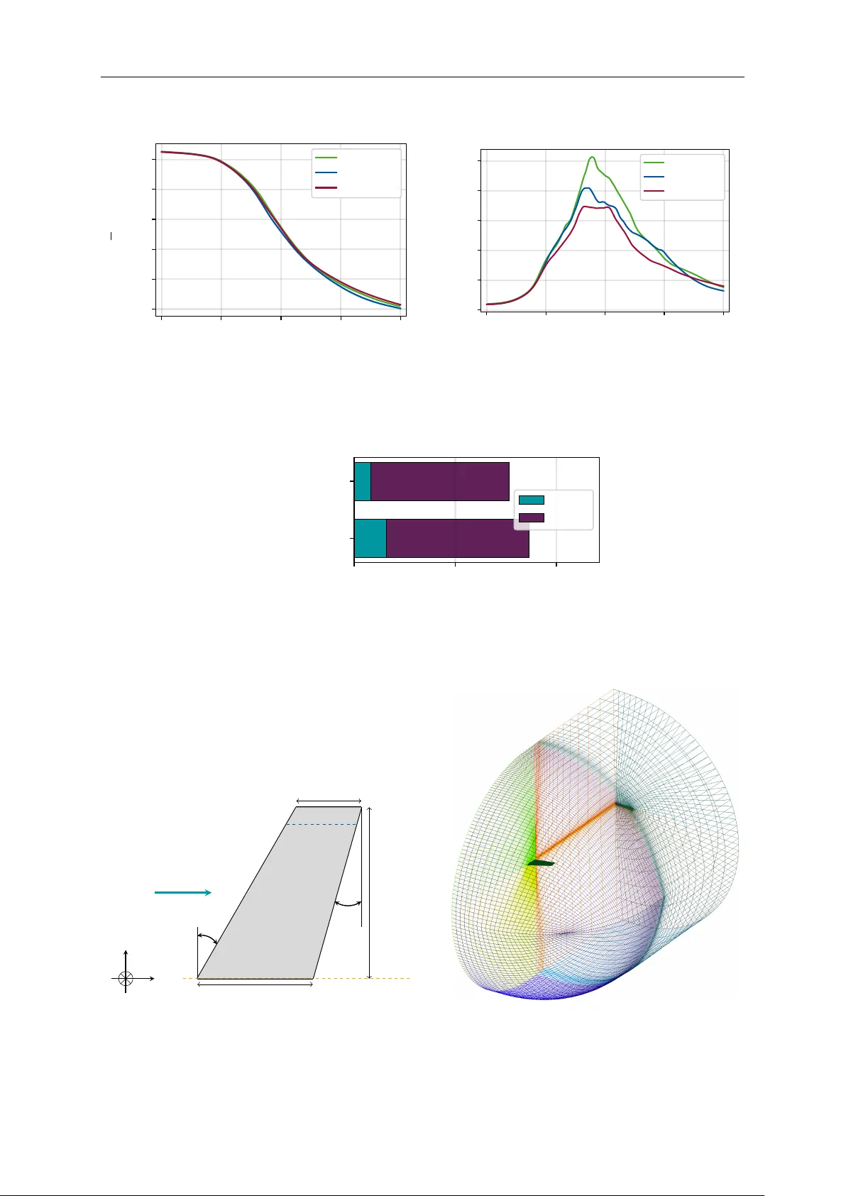
V olume T erm A daptivit y for Discon tin uous Galerkin Sc hemes Daniel Do ehring a, ∗ , Jesse Chan b , Hendrik Rano c ha c , Mic hael Schlottk e–Lak emp er d , Man uel T orrilhon a , and Gregor Gassner e a Applie d and Computational Mathematics, R WTH A achen University, Germany. b Oden Institute for Computational Scienc e and Engine ering, A er osp ac e Engine ering & Engine ering Me chanics, University of T exas at A ustin, USA. c Institute of Mathematics, Johannes Gutenb er g University Mainz, Germany. d High-Performanc e Computing, Center for A dvanc ed A nalytics and Pr e dictive Sciences, University of A ugsbur g, Germany. e Dep artment of Mathematics and Computer Scienc e, Center for Data and Simulation Scienc e, University of Colo gne, Germany. Abstract W e in troduce the concept of v olume term adaptivit y for high–order discon tin uous Galerkin (DG) sc hemes solving time–dep endent partial diﬀeren tial equations. T ermed v –adaptivity , w e presen t a no v el general approac h that exc hanges the discretization of the volume con tribution of the DG sc heme at every R unge–Kutta stage based on suitable indicators. Dep ending on whether robustness or eﬃciency is the main concern, diﬀeren t adaptation strategies can b e c hosen. Precisely , the w eak form v olume term discretization is used instead of the en trop y- conserving ﬂux–diﬀerencing v olume in tegral whenev er the former pro duces more en trop y than the latter, resulting in an entrop y–stable scheme. Conv ersely , if increasing the eﬃciency is the main ob jective, the weak form v olume in tegral ma y b e employ ed as long as it do es not increase en tropy b ey ond a certain threshold or cause instabilities. Th us, dep ending on the choice of the indicator, the v –adaptive DG sc heme impro ve s robustness, eﬃciency and appro ximation qualit y compared to schemes with a uniform volume term discretization. W e thoroughly verify the accuracy , linear stability , and entrop y–admissibilit y of the v –adaptiv e DG scheme before applying it to v arious compressible ﬂow problems in tw o and three dimensions. K eywor ds: Discontin uous Galerkin, A daptive Metho ds, High–Order, Entrop y Stability 2020 MSC: 65M60, 65M70, 65M50, 76-04 1. In tro duction A daptivity is a necessit y for the feasible simulation of complex ph ysical phenomena with high–ﬁdelit y , high–order metho ds. When referring to adaptivity , we mean the ability of a n u- merical method to automatically adjust the discretization technique to the current lo cal solution appro ximation ov er the course of the simulation. A daptivity is a well–kno wn concept in the nu- merical treatment of partial diﬀerential equations (PDEs) and has b een studied extensiv ely in the past decades. Established terms are h–adaptivity , often also referred to as adaptiv e mesh reﬁnemen t (AMR) [1–5], where the cell size is lo cally adjusted to capture small–scale features of the solution, for instance sho ck fron ts and b oundary lay ers. Next, p–adaptivity [6–10] refers to the local adjustmen t of an elemen t’s p olynomial degree p which is particularly useful to capture smo oth solution features with high accuracy , such as v ortical structures in turbulent ﬂo ws. Third, r–adaptivity [11–14] denotes metho ds where the cells are mov ed and deformed to b etter align them with solution features such as discontin uities. A daptivit y of the appro xi- mating scheme similar to the this w ork has also b een explored. Some examples related to the ∗ Corresp onding author V olume T erm Adaptivit y for Discon tinuous Galerkin Schemes presen t work are order adaptation [15–22], order–preserving stabilization [23–28] and explicit sho c k–capturing strategies [21, 22, 29]. F urthermore, for time–dep enden t problems solv ed with explicit time in tegrators, adaptive strategies to alleviate the time step restriction imp osed b y the Couran t–F riedric hs–Lewy (CFL) condition hav e b een developed. Classic examples thereof are lo cal time stepping [2, 3, 30, 31] whic h reduce the timestep lo cally p er cell, and multirate time in tegration metho ds [32–36] which emplo y metho ds with enlarged regions of absolute stability for cells with more restricted timestep sizes. Finally , w e would lik e to remark that adaptivit y is not limited to discretization tec hniques, but is also extended to the mo deling itself, i.e., diﬀeren t ph ysical mo dels are employ ed in dynamically adapted regions of the domain, see for instance [37–41] and references therein. In this work, we fo cus on Discon tinuous Galerkin (DG) metho ds [42–44] and their applica- tion to time–dep enden t hyperb olic–parab olic PDEs, mos t notably the compressible Euler and Na vier–Stokes–F ourier equations. A standard weak/v ariational formulation of a PDE with a DG discretization consists of tw o main parts: The surface term and the volume term, whic h arise from the application of in tegration b y parts to the in tegrated PDE. The treatmen t of the surface term b oils down to the numerical solution of Riemann problems at elemen t inter- faces, for which a wealth of approximate Riemann solvers/n umerical ﬂux functions is av ailable [5, 45–49]. The treatment of the volume term, how ev er, leav es more freedom in the design of the numerical scheme. This ﬂexibilit y is crucial to obtain en tropy–conserv ativ e/entrop y–stable (EC/ES) [50–52] DG sc hemes which emplo y a sp ecial type of volume term discretization, the so–called ﬂux–diﬀer encing (FD) form [23, 24, 53–56], which greatly enhances the stabilit y of these metho ds [27, 57–60]. In general, the usage of the (in general) more robust EC/ES DG sc hemes comes at the cost of a more in volv ed v olume term discretization. In particular, for the FD form, the v olume term ev aluation requires the computation of sp ecial tw o–point ﬂux functions at pairs of the quadrature no des of the element. This is esp ecially troubling for element t yp es which do not naturally p os- sess a tensor–pro duct/sum factorization structure, such as triangles, tetrahedra, pyramids, and prisms unless sp ecialized tec hniques are employ ed, see for instance [61] and references therein. But even for tensor–pro duct elements such as quadrilaterals and hexahedra, the FD form is for higher p olynomial degrees more exp ensiv e than a standard weak form (WF) volume in tegral, whic h only in volv es a single analytical ﬂux ev aluation p er quadrature no de. This observ ation serv es as the main motiv ation for this work: W e seek to use the cheaper w eak form v olume term as often as p ossible, with the option to switch to the more exp ensiv e FD form only when necessary to retain stability of the simulation. The choice of the v olume term discretization is made lo cally p er element and R unge–Kutta stage based on a suitable indicator, which ma y b e of a–priori or a–p osteriori nature. This gives rise to a new t yp e of adaptivit y for DG sc hemes, whic h we refer to as volume term– or in short v–adaptivity . In some sense, this idea is a gener- alization of the approac h tak en in [21, 22] wherein the entrop y–conserv ative FD v olume in tegral is blended with a low er–order ﬁnite volume sc heme deﬁned on the DG sub cells to pro vide stabi- lization. A blueprint for the a–p osteriori adaptivity are the works on multi-dimensional optimal order detection (MOOD) [15–17] and its extension to DG sc hemes [18–20], where the solution is c heck ed after computation for admissibility given by certain indicators and adjusted otherwise. Another related approach is prop osed in [23, 24] where the ﬁnite–diﬀerence scheme is equipp ed with a more stable ﬁnite–v olume discretization to stabilize the simulation. In a recen t work [27] the authors prop osed combining the standard DG weak form with the entrop y stable DG sc heme from [62] on Gauss–Legendre p oin ts based on the indicator from [21, 63]. W e generalize this approac h to general quadrature rules and general indicators. Besides enhancing eﬃciency , it is also p ossible to imp ro v e the robustness of the discretization b y using the WF up date for an elemen t whenev er it dissipates more en trop y than the FD v olume term/v olume in tegral (VT/VI) on that element, which is a rigorous criterion for en tropy– stabilit y/diﬀusion. The key to eﬃciency for this approac h is that one can compute the analytical 2 Do ehring et al. elemen t–wise entrop y pro duction, which is identical to the entrop y pro duction of the FD VT/VI, without the need to compute the FD v olume term itself. Instead, only the element–wise surface in tegral of the entrop y p otential is required [28, 29, 55, 56]. The paper is structured as follo ws: W e begin b y reviewing the classic WF and EC/ES FD volume term discretizations of DG schemes in Section 2. Next, in Section 3 we presen t an indicator based on the element–wise entrop y pro duction rate to determine the appropriate v olume term. In particular, we d evise a simple rigorous entrop y–stable criterion that increases robustness of the simulation, and a heuristic criterion that aims to reduce computational cost without impairing stabilit y signiﬁcan tly . A dditionally , we brieﬂy revisit the indicator from [21, 63] as this will also b e used to demarcate b etw een the WF and the ﬁnite v olume (FV)–stabilized FD volume term (VT). In Section 4 we v erify the newly obtained entrop y–dissipativ e adaptive v olume in tegral in terms of order of accuracy , linear stability , and entrop y–stabilit y . Examples for coupling the WF with pure FD and stabilized FD–FV are presented in Section 5, b efore we conclude the w ork in Section 6. 2. V olume T erm F orm ulations in No dal Discon tin uous Galerkin Schemes In this section, w e brieﬂy review the ma jor steps in the construction of the EC/ES DG sc hemes based on the FD form. W e restrict ourselves here for simplicit y to the discon tinu- ous Galerkin sp ectral element metho d (DGSEM) [44, 64, 65] with collo cated Gauss–Legendre– Lobatto in terp olation/quadrature no des on tensor–pro duct elemen ts. The interested reader is referred to [56, 60, 66–68] for more general choices of the quadrature rule and to [55, 62, 69] for a discussion on mo dal and non tensor–pro duct elemen ts. 2.1. W e ak F ormulation of the 1D Disc ontinuous Galerkin Sp e ctr al Element Metho d Consider the v ector–v alued conserv ation law in one spatial dimension ∂ t u ( t, x ) + ∂ x f ( u ) = 0 , (2.1) whic h can b e transformed from a physical element Ω i = [ x i − 1 / 2 , x i + 1 / 2 ] to the reference element b Ω : = [ − 1 , 1] via the aﬃne mapping ξ ( x ) : = 2 x − x i − 1 / 2 x i + 1 / 2 − x i − 1 / 2 − 1 , x ∈ Ω i (2.2) and in verse x i ( ξ ) : = x i − 1 / 2 + x i + 1 / 2 − x i − 1 / 2 2 ( ξ + 1) , ξ ∈ b Ω (2.3) with the Jacobian of the transformation J i : = ∂ x i ( ξ ) ∂ ξ = x i + 1 / 2 − x i − 1 / 2 2 . (2.4) Th us, the conserv ation law in reference space reads ∂ t u  t, x i ( ξ )  + ∂ ξ ∂ ξ ∂ ∂ x f  u ( t, x i ( ξ ))  = 0 (2.5a) ⇔ ∂ t u  t, x i ( ξ )  + J − 1 i ∂ ∂ ξ f  u ( t, x i ( ξ ))  = 0 (2.5b) ⇔ J i ∂ t u  t, x i ( ξ )  + ∂ ξ f  u ( t, x i ( ξ ))  = 0 . (2.5c) W e expand the solution u in terms of Lagrange p olynomials ℓ j ( ξ ) of degree p deﬁned on the Gauss–Lobatto no des ξ 0 , . . . , ξ p ∈ b Ω as u ( t, x i ( ξ )) : = p X j =0 u i,j ( t ) ℓ j ( ξ ) , (2.6) 3 V olume T erm Adaptivit y for Discon tinuous Galerkin Schemes with time–dep enden t degrees of freedom u i,j ( t ) which are deﬁned for every element Ω i and no de j = 0 , . . . , p . W e insert this expansion in to (2.5c) and make the traditional Galerkin ansatz b y multiplying with test functions identical to ansatz functions ℓ k ( ξ ) and integrating o ver the reference elemen t b Ω to obtain 0 = Z 1 − 1  J i ∂ t u  t, x i ( ξ )  + ∂ ξ f ( u )  ℓ k ( ξ ) dξ , k = 0 , . . . , p (2.7a) = J i Z 1 − 1 ∂ t u  t, x i ( ξ )  ℓ k ( ξ ) dξ + Z 1 − 1 ∂ ξ f ( u ) ℓ k ( ξ ) dξ , k = 0 , . . . , p . (2.7b) The ﬁrst term in (2.7b) can b e simpliﬁed by inserting (2.6) J i Z 1 − 1 ∂ t u  t, x i ( ξ )  ℓ k ( ξ ) dξ = J i Z 1 − 1 p X j =0 ∂ t u i,j ( t ) ℓ j ( ξ ) ℓ k ( ξ ) dξ (2.8a) = J i p X l =0 ω l p X j =0 ∂ t u i,j ( t ) ℓ j ( ξ l ) ℓ k ( ξ l ) (2.8b) with ω l denoting the quadrature weigh ts of the Gauss–Lobatto quadrature rule. Due to the collo cation prop ert y of the Lagrange p olynomials, i.e., ℓ j ( ξ l ) = δ j k , (2.8b) simpliﬁes to J i Z 1 − 1 ∂ t u  t, x i ( ξ )  ℓ k ( ξ ) dξ = J i ω k ∂ t u i,k ( t ) = J i ω k ˙ u i,k ( t ) (2.9) whic h is can b e expressed in matrix notation with diagonal mass matrix M ij : = δ ij ω i , i, j = 0 , . . . , p (2.10) as J i Z 1 − 1 ∂ t u  t, x i ( ξ )  ℓ k ( ξ ) dξ = J i M ˙ u i ( t ) (2.11) where w e assemble the co eﬃcients u i,j ( t ) at quadrature no des j into u i ( t ) : =    u i, 0 ( t ) . . . u i,p ( t )    . (2.12) Next, w e consider the second summand in (2.7b) and apply integration by parts to obtain Z 1 − 1 ∂ ξ f ( u ) ℓ k ( ξ ) dξ =  f  u ( t, x i ( ξ ))  ℓ k ( ξ )  1 − 1 − Z 1 − 1 f ( u ) ℓ ′ k ( ξ ) dξ . (2.13) The ﬁrst term on th e right–hand side of (2.13) represen ts the interface or surfac e term of the DG sc heme which simpliﬁes with ℓ k ( − 1) = δ k 0 and ℓ k (1) = δ kp to  f  u ( t, x i ( ξ ))  ℓ k ( ξ )  1 − 1 = f  u ( t, x i + 1 / 2 )  δ kp − f  u ( t, x i − 1 / 2 )  δ k 0 . (2.14) Analogous to FV schemes, the ph ysical ﬂux ev aluations at element interfaces with p oten tially discon tinuous states u  t, x L i ± 1 / 2   = u  t, x R i ± 1 / 2  are replaced b y n umerical ﬂux functions f ⋆ whic h approximate the solution of the Riemann problem. By in tro ducing the b oundary matrix B : =       − 1 0 · · · 0 0 0 · · · 0 . . . . . . . . . . . . 0 0 · · · 1       (2.15) 4 Do ehring et al. w e can further simplify (2.14) to  f  u ( t, x i ( ξ ))  ℓ k ( ξ )  1 − 1 = B         f ⋆ | − 1 0 . . . 0 f ⋆ | 1         = : B f ⋆ i . (2.16) Finally , w e come to the volume term in (2.13) for whic h we apply the quadrature rule to obtain − Z 1 − 1 f ( u ) ℓ ′ k ( ξ ) dξ = − p X l =0 ω l f  u ( t, x i ( ξ l ))  ℓ ′ k ( ξ l ) . (2.17) With the derivative matrix D ij : = ℓ ′ j ( ξ i ) , i, j = 0 , . . . , p (2.18) and mass matrix from (2.10), we can express the volume term in matrix notation as − Z 1 − 1 f ( u ) ℓ ′ k ( ξ ) dξ = − D T M f i k = 0 , . . . , p (2.19) whic h gives the complete weak form DG semidiscretization in reference space on element Ω i as J i M ˙ u i ( t ) + B f ⋆ i − D T M f i = 0 (2.20a) ⇔ J i ˙ u i ( t ) = − M − 1 B f ⋆ i + M − 1 D T M f i . (2.20b) 2.2. Flux–Diﬀer encing F ormulation of the 1D Disc ontinuous Galerkin Sp e ctr al Element Metho d F or the sak e of notational compactness we drop the elemen t index i in the following. A crucial observ ation for the construction of EC/ES DG schemes is that the mass, b oundary , and deriv ative matrices fulﬁll the summation–by–p arts (SBP) pr op erty [53, 70–74] MD | {z } = : Q +( MD ) T = B . (2.21) Emplo ying this prop erty , one can rewrite D T M = D T M T = ( MD ) T = B − MD and thus express the v olume term as M − 1 D T M f = M − 1 ( B − MD ) f (2.22) whic h can b e group ed into b oundary and volume contributions as M − 1 D T M f = M − 1 B f − D f . (2.23) The key insigh t from [23] is that if the deriv ativ e op erator D fulﬁlls a telescoping prop ert y , i.e., ev ery row sums to zero, one can rewrite  D f  j = p X k =0 D j,k f k = p X k =0 D j,k f k + f j p X k =0 D j,k | {z } = 0 = 2 p X k =0 1 2 D j,k  f j + f k  (2.24) whic h is the FD form of the volume term. Note that the WF v olume in tegral is equiv alen t to the FD volume integral with the central tw o–p oin t ﬂux employ ed as the volume ﬂux . Replacing the cen tral tw o–point ﬂux f Central  f j , f k  = 1 2  f j + f k  (2.25) 5 V olume T erm Adaptivit y for Discon tinuous Galerkin Schemes T able 1: Mean runtimes τ for the ev aluation of the analytical compressible Euler ﬂux and the tw o–p oint entrop y– conserv ativ e ﬂuxes by Chandrashekar [76] and Rano cha [78] in one, t wo, and three spatial dimensions. τ [ns] 1D 2D 3D Analytical 2 . 1 2 . 3 2 . 3 Chandrashekar [76] 11 . 8 13 . 5 14 . 8 Rano c ha [78] 10 . 1 12 . 0 12 . 3 with an appropriate entrop y–conserv ative and consistent tw o–point ﬂux function f EC ( u j , u k ) [75–79] leads to an entrop y–conserv ative volume term discretization [54]. W e thus replace − D f in (2.23) by − 2 D f EC and reformulate the DG scheme (2.20b) using the ab o ve manipulations as J ˙ u ( t ) = − M − 1 B f ⋆ + M − 1 B f EC − D f EC (2.26a) = − M − 1 B  f ⋆ − f EC  − 2 D f EC (2.26b) = − M − 1 B f ⋆ −  2 D − M − 1 B  f EC . (2.26c) The matrix D split : = 2 D − M − 1 B is t ypically referred to as derivative–split matrix [54]. A closer insp ection of (2.24) rev eals why the FD approac h is computationally more exp ensiv e than the WF volume term. The WF volume term requires d · ( p + 1) d analytical/ph ysical ﬂux ev aluations to construct f in d spatial dimensions. In contrast, the FD discretization requires dp / 2 · ( p + 1) d t wo–point numerical ﬂux ev aluations p er elemen t, i.e., there is quadratic gro wth in the num b er of entrop y–conserv ative (EC) ﬂux ev aluations with increasing p olynomial degree p . The ratio of ﬂux ev aluations b etw een the FD and WF volume terms is thus for all d given by p / 2 . In other words, if the WF VT would b e naively implemen ted in FD form, the simulation would b e ab out p / 2 times more exp ensive and take corresp ondingly longer solely due to the increased n umber of ﬂux ev aluations. F or non–tensor pro duct/sum factorization elements, though, the situation is dramatically w orse, as now t w o–p oint ﬂuxes need to be ev aluated betw een all pairs of no des within an elemen t. F or an element with N no des, this results in N f = N − 1 X j =1 j = 1 2 N ( N − 1) (2.27) ﬂux ev aluations p er element. Assuming now that the num ber of no des N scales with the p oly- nomial degree p as N ∼ p d , we obtain a scaling of N f ∼ p 2 d whic h is muc h worse than the p d +1 scaling for tensor–pro duct elemen ts. A dditionally , the computation of the en trop y–conserving tw o–point ﬂuxes is more expen- siv e than the analytical ﬂux ev aluation. While the analytical/physical ﬂux can b e computed using the most basic arithmetic op erations, the computation of the EC ﬂuxes inv olv es usually some logarithmic means [75–78] which considerably increase the computational cost per ﬂux ev aluation. T o illustrate this, w e present runtimes for the ev aluation of the analytical ﬂux and the EC ﬂux by Chandrashekar [76] and Rano cha [78] as implemented in Trixi.jl [80–82] for the compressible Euler equations in T able 1. The measurements are obtained for a veraging o ver all directions i = 1 , . . . , d and 10 7 ev aluations for blast–alike initial states ρ l = ρ r = 1 , v l = v r = 0 , p l = 10 4 , and p r = 1 . F or the analytical ﬂux, the tabulated v alue is the av erage of f ( u l ) , f ( u r ) . Clearly , the EC ﬂuxes are about 1 . 4 to 1 . 6 times more exp ensive than the analytical ﬂux ev aluation. 6 Do ehring et al. 3. Indicator T o decide which v olume term discretization to use in the v –adaptive framework, a suitable indicator is required. F or the com bination of the weak form and ﬂux–diﬀerencing form v olume terms w e prop ose an indicator based on the cell–wise en trop y pro duction of the numerical sc heme. In particular, one can compute the change in mathematical entrop y S ( u ) as ˙ S = ∂ t S  u ( t )  = ∂ S ∂ u ∂ t u ( t ) = w T ˙ u (3.1) where we introduced the entrop y v ariables w : = ∂ S ∂ u [52]. The entrop y pro duction due to the VT can th us b e computed as ˙ S | WF = w T · ˙ u | WF (2.20b) = − J − 1 M − 1 D T M f (3.2a) ˙ S | FD = w T · ˙ u | FD (2.26c) = − J − 1  2 D − M − 1 B  f EC . (3.2b) The discrete scheme satisﬁes a cell entrop y inequality if w e can b ound the entrop y pro duction of the v olume term by the surface integral of the entr opy p otential ψ [28, 29, 55, 56] ˙ S | VT ≤ Z ∂ Ω ψ ( u ) d S = [ ψ ( u )] +1 − 1 (3.3) and entrop y–dissipativ e surface ﬂuxes f ⋆ are employ ed. The entrop y p otential ψ [52] is deﬁned via the relation ψ  w ( u )  : = w T f ( u ) − F ( u ) (3.4) where F ( u ) is the entr opy ﬂux deﬁned via [52]  ∂ F ∂ u  T = w T  ∂ f ∂ u  . (3.5) The (comp onent–wise) entrop y p otential for the compressible Euler equations is given simply b y the momentum comp onents, i.e., in one dimension ψ ( u ) = ρv [52]. 3.1. R igor ous Indic ator for mor e R obust Entr opy–Stable Schemes W e now turn our atten tion to designing a numerical scheme that is globally en tropy dissi- pativ e b y com bining the WF and FD VT discretizations. In particular, we seek to construct a more stable adaptive scheme b y using the WF volume term if it in tro duces more deca y in the mathematical en tropy than the FD form, i.e., if ∆ S i : = ˙ S i | WF − ˙ S i | FD < 0 (3.6) for element Ω i . This w ay , we obtain a globally entrop y–stable scheme (assuming the surface terms dissipate en tropy) as we only use the WF volume term when it is more dissipativ e than the FD form. A related approach for the en tire semidiscretization, i.e., not only the volume in tegral, w as already suggested in [24] where also an adaptive sc heme based on lo cal entrop y pro duction was presented. In particular, the authors suggest equipping an entrop y–conserv ative sc heme with an entrop y–diﬀusiv e c omp anion scheme and blending them based on lo cal en tropy pro duction. In [24] WENO and other ﬁnite volume based sc hemes are suggested as companion sc hemes, with the former b eing employ ed in [23]. Thus, in the terminology of [24], the herein presen ted approach uses the WF/central–ﬂux FD volume integral as the diﬀusive c omp anion sc heme for the en trop y–conserving FD v olume in tegral. Other closely related works are the a–p osteriori sub cell limiting DG schemes developed in [18–20] which are based on the MOOD paradigm [15–17]. A daptiv e or switching schemes, alb eit not necessarily for entrop y–stabilit y , ha ve also b een studied in [83–85], for instance. 7 V olume T erm Adaptivit y for Discon tinuous Galerkin Schemes The indicator as presen ted in (3.6) is unfortunately very exp ensive, as the FD volume term is alwa ys computed, even if it is not used in the ﬁnal up date. As p ointed out in [28, 29], this can b e a voided by replacing ˙ S i | FD b y ˙ S i | FD = ψ  u i,p  − ψ  u i, 0  . (3.7) Emplo ying this in the indicator equation (3.6) thus gives ∆ S i : = ˙ S i | WF −  ψ  u i,p  − ψ  u i, 0   < 0 . (3.8) This wa y , we only need to compute the entrop y pro duction of the WF volume term and the surface in tegral of the entrop y p oten tial to ev aluate the indicator. The FD volume term is in this case only computed if entrop y is indeed increasing. W e remark that in the case where for a ma jority of cells the WF VT may b e used, this is not only a more robust scheme, but also more eﬃcien t scheme for p olynomial degrees p > 2 as the FD volume term is only computed on a subset of elemen ts. The indicator (3.8) is computed at ev ery Runge–Kutta stage and element in the v –adaptiv e framew ork. Note that this indicator is of a–p osteriori nature, as the WF VT is computed in an y case, but p oten tially discarded. W e present numerical results for this scheme show casing increased robustness o ver the pure FD form in Section 5. 3.2. Heuristic Indic ator for mor e Eﬃcient Schemes If eﬃciency is the main concern for a simulation, one can relax the indicator by in tro ducing an upp er b ound σ i for the tolerated entrop y pro duction of the WF volume term. In particular, the WF v olume term is used if ˙ S i, WF < σ i . (3.9) The WF v olume integral serves in this case as a predictor, and correction via the FD volume in tegral is only applied if deemed necessary by the indicator. The diﬃculty lies no w in ﬁnding a reasonable upp er b ound σ i for the admissible en tropy pro- duction of the WF volume term. Is this b ound to o large, the WF v olume integral is p otentially applied to o often, leading to instabilities. On the other hand, if the b ound is to o small, the FD v olume term computation is used most of the time, leading to ultimately higher computational cost than a pure FD scheme. W e emphasize here that σ applies to the entrop y pro duction in reference space, which eliminates issues with magnitude across elements of diﬀerent sizes and enables b etter reusabilit y of the parameter across diﬀerent meshes. W e exp erimen ted with diﬀer- en t ﬁxed and dynamic b ounds, the latter computed from the erronous total en tropy pro duction ˙ S > 0 observed for a complete R unge–Kutta step. In practice, the dynamic approach did not yield improv emen ts ov er a ﬁxed b ound, and thus we present results only for the latter case in Section 5. Similar to identifying a stable CFL num ber, w e determined a stable σ by p erforming bisection starting with e.g. σ max = 10 − 2 and σ min = 0 . 0 . More sophisticated approaches are left for future w ork. 3.3. Sho ck–Capturing Indic ator In the case where the w eak form v olume term is combined with the stabilizing blended DG–FV we typically emplo y the a–priori troubled–cell indicator from [21, 63]. The indicator con verts the no dal representation in Lagrange p olynomials into a mo dal represen tation in terms of orthogonal Legendre p olynomials via m = V ( ξ ) − 1 v (3.10) with V ( ξ ) denoting the V andermonde matrix of the Legendre polynomials ev aluated at the in terp olation no des ξ = { ξ 0 , . . . , ξ p } . Note that v = { v j } in (3.10) is the no dal representation 8 Do ehring et al. of an indicator quan tity such as density ρ , pressure p , or the pro duct of these tw o ρ · p . F rom the mo dal co eﬃcien ts m the energies E n : = p − n X j =0 m 2 j , n = 0 , 1 , 2 (3.11) are computed. The inﬂuence of the higher mo des, i.e., p otential oscillations, is then measured b y the fractions ε 0 : = E 0 − E 1 E 0 , ε 1 : = E 1 − E 2 E 1 (3.12) from which the maximum ε : = max( ε 0 , ε 1 ) is computed. Then, the blending factor β is computed from the standard logistic function as β : = 1 1 + exp  − κ ε −T T  (3.13) with h yp erparameters κ : = log 1 − 10 − 4 10 − 4 ! ≈ 9 . 21024 , T : = 0 . 5 · 10 1 . 8 · p 0 . 25 . (3.14) T o a void unnecessary blending in the case of a very small β , a threshold β min ≥ 0 is supplied, b elo w which the indicator v alue is clipp ed to zero. Similarly , one can limit the maxim um blending factor to β max ≤ 1 to a void excessive blending in the case of a very large β : β =        0 β < β min β β min ≤ β ≤ β max β max β > β max . (3.15) The indicator is computed at every Runge–Kutta stage and element in the blended DG–FV framew ork with indicator v ariable v taken from the previous Runge–Kutta stage. Thus, the blending is determined a–priori an y volume term computations of the current stage. 3.3.1. Sho ck–Capturing via Blende d DG–FV The blended DG–FV sc heme uses a conv ex combination of a high–order DG discretization and a non–oscillatory ﬁrst or second–order FV discretization in troubled cells identiﬁed by the sho c k indicator β . The volume term up date is then given by ˙ u i | DG–FV : = (1 − β i ) ˙ u i | FD + β i ˙ u i | FV , β i ∈ [0 , β max ] , (3.16) where ˙ u i | FV is a standard ﬁnite–volume up date on the sub cells of the [ − 1 , 1] d reference element. The blending p ar ameter β i determines the amount of dissipation in tro duced b y the FV up date. F or a p –degree DG scheme, ( p + 1) d sub cells are used p er elemen t in d spatial dimensions. The natural size of these sub cells is given b y the quadrature weigh ts ω i of the Lobatto–Legendre basis [21]. Th us, the ﬁrst sub cell is given by [ − 1 , − 1 + ω 1 ] , the second b y [ − 1 + ω 1 , − 1 + ω 1 + ω 2 ] , and so on. The sc heme (3.16) is prov ably entrop y stable and the main sho ck–capturing metho dology used in Trixi.jl [80 – 82]. 3.4. Combining Sho ck–Capturing and Entr opy–Pr o duction Indic ators Due to the diﬀerent nature (a–priori vs a–p osteriori) of the sho ck–capturing and v –adaptive indicators, they can b e readily combined to give a nested VT computation strategy . In particular, the sho ck–capturing indicator is computed ﬁrst to decide whether any stabilization via blended DG–FV is required. If not, the VT for this elemen t is computed with the weak form, and the 9 V olume T erm Adaptivit y for Discon tinuous Galerkin Schemes 16 32 64 128 256 N x = N y 10 − 8 10 − 7 10 − 6 10 − 5 10 − 4 10 − 3 e L 2 ρ (Isentropic Vo rtex) Adaptive Weak Fo rm Flux–Diﬀ. O  ∆ x 4  (a) Domain–normalized L 2 error in density . 16 32 64 128 256 N x = N y 10 − 6 10 − 5 10 − 4 10 − 3 10 − 2 e L ∞ ρ (Isentropic Vo rtex) Adaptive Weak Fo rm Flux–Diﬀ. O  ∆ x 4  (b) Poin t wise L ∞ error in density . Figure 1: Errors of the isen tropic vortex advection testcase with viscous surface ﬂux. v –adaptive indicator is ev aluated to decide whether the FD volume term is required for this elemen t to maintain e.g. entrop y stabilit y . In practice, ho w ev er, w e ha ve for the DGSEM (i.e., tensor–pro duct elemen ts) not f ound examples where this hybrid strategy is more eﬃcient to main tain EC/ES prop erties than using alw ays the FD volume term in non–stabilized regions. W e b eliev e that this hybrid strategy could b e b eneﬁcial for non tensor–pro duct elements where the cost of the FD volume term is m uch higher than the WF v olume term, but this is left for future work. 4. V eriﬁcation All numerical tests and examples are p erformed with Trixi.jl [80–82], a high–order DG co de written in Julia [86] for the n umerical sim ulation of transp ort–dominated h yp erb olic– parab olic balance laws and related multiph ysics problems. All computations p erformed in this section can b e repro duced without the need for commercial and proprietary softw are. The ﬁles to repro duce the results are publicly a v ailable on GitHub and arc hived on Zenodo [87]. 4.1. Conver genc e 4.1.1. Isentr opic V ortex A dve ction with V isc ous Surfac e Flux W e consider the isentropic vortex adv ection problem [88, 89] using the Harten–Lax–V an Leer–Con tact (HLLC) interface ﬂux [48] and the en tropy-conserv ativ e, kinetic energy-preserving v olume ﬂux describ ed by Rano c ha [79]. The p olynomial degree is set to p = 3 and the v ortex setup follows the conﬁguration from [35]. The simulation in volv es a single pass of the vortex through the computational domain. W e consider four reﬁnemen ts of the computational domain, starting with 2 4 × 2 4 elemen ts up to 2 8 × 2 8 elemen ts. W e consider the WF, FD, and the v –adaptive scheme with rigorous indicator from Section 3. Domain–normalized L 2 error and p oin twise L ∞ error in density are depicted in Fig. 1. The exp ected asymptotic conv ergence rates are observ ed for all schemes, while the low est errors are ob tained with the FD v olume term discretization. 4.1.2. Density W ave with Inviscid Surfac e Flux As a ﬁrst v eriﬁcation we consider the 1D density wa v e test case from [90] giv en by ρ ( x ) = 1 + 0 . 98 sin  2 π x  (4.1a) v x ( x ) = 0 . 1 (4.1b) p ( x ) = 20 (4.1c) 10 Do ehring et al. 4 8 16 32 64 128 256 N x 10 − 1 10 − 2 10 − 3 10 − 4 10 − 5 10 − 6 10 − 7 e L 2 ρ (Density Wave) Adaptive Flux–Diﬀ. O  ∆ x 4  O  ∆ x 3  (a) Domain–normalized L 2 error in density . 4 8 16 32 64 128 256 N x 10 − 6 10 − 5 10 − 4 10 − 3 10 − 2 10 − 1 e L ∞ ρ (Density Wave) Adaptive Flux–Diﬀ. O  ∆ x 4  O  ∆ x 3  (b) Poin t wise L ∞ error in density . Figure 2: Errors for the densit y wa ve conv ergence testcase with inviscid surface ﬂux. on Ω = [ − 1 , 1] with p erio dic b oundary conditions. The compressible Euler equations reduce for this setup to a linear advection equation for the density ρ with v elo city v x = 0 . 1 . F or the purp ose of this testcase, we emplo y the inviscid EC tw o–p oin t ﬂux by Rano c ha [79] for b oth the surface ﬂux and the volume ﬂux in the FD v olume term discretization. The solution p olynomials are discretized with p olynomial degree p = 3 and the simulation is adv anced up to t f = 2 using the ﬁv e–stage, fourth–order low–storage Runge–Kutta metho d from [91]. In contrast to the previous example, where the FD discretization yielded the low est errors, w e observ e here that the adaptive, entrop y–dissipativ e discretization (i.e., with rigorous indicator) leads to lo wer errors for b oth L 2 and L ∞ norms as depicted in Fig. 2. The WF discretization is not depicted here as it is unstable for this conﬁguration. Notably , only the adaptive sc heme reco vers fourth–order conv ergence in L ∞ norm, while the pure EC sc heme only yields third–order con vergence. 4.2. Line ar Stability In [90] linear stabilit y defects of en tropy–conserv ativ e FD volume term discretizations were analyzed. In particular, it w as shown that for certain conﬁgurations of the DGSEM the en tropy– conserv ative FD volume term leads to linearly unstable sc hemes, ev en when paired with dissi- pativ e in terface ﬂuxes. Here, we focus on the tw o–dimensional density w av e example with conﬁguration from [90] giv en by ρ ( x, y ) = 1 + 0 . 98 sin  2 π ( x + y )  (4.2a) v x ( x, y ) = 0 . 1 (4.2b) v y ( x, y ) = 0 . 2 (4.2c) p ( x, y ) = 20 (4.2d) on Ω = [ − 1 , 1] 2 with p erio dic b oundary conditions. The compressible Euler equations reduce for this setup to a linear advection equation for the densit y ρ with v elo city v = (0 . 1 , 0 . 2) T . The solution is discretized using 4 × 4 quadrilateral elements of p olynomial degree p = 5 with the R usanov/local Lax–F riedrichs (LLF) ﬂux [45] and the entrop y–conserv ative volume ﬂux from Chandrashekar [76]. This setup is delib erately chosen to b e sensitive to p erturbations in densit y , whic h p ose the danger to violate p ositivity . The desired ﬁnal time is t f = 5 . 0 , timestepping is p erformed with the explicit fourth–order, ﬁve–stage lo w–storage R unge–Kutta metho d from [91]. The timestep is computed from the CFL condition ∆ t = CFL 1 ( p + 1) min i ∆ x i λ i (4.3) 11 V olume T erm Adaptivit y for Discon tinuous Galerkin Schemes − 4 − 3 − 2 − 1 0 1 2 3 4 Re 0 20 40 60 80 100 120 140 Im σ ( J ) of Adaptive VT/VI (a) Adaptiv e − 4 − 3 − 2 − 1 0 1 2 3 4 Re 0 20 40 60 80 100 120 140 Im σ ( J ) of WF VT/VI (b) WF − 4 − 3 − 2 − 1 0 1 2 3 4 Re 0 20 40 60 80 100 120 140 Im σ ( J ) of FD VT/VI (c) FD Figure 3: Sp ectra at initial time t = 0 for the linear stability testcase. 0 1 2 3 4 5 t − 0.03 − 0.02 − 0.01 0.00 S ( t ) − S ( t 0 ) Adaptive Flux–Diﬀ. Weak Fo rm Figure 4: En tropy diﬀerence ov er time for the densit y wa v e linear stability testcase with rigorous indicator for the adaptive volume term discretization. The simulations are p erformed with CFL = 0 . 9 . where λ denote the wa v e sp eeds λ ∈ σ ( ∂ u f ) and ∆ x is a suitable measure for the lo cal element size. The minimum is taken ov er all elements and their interpolation p oints. As demonstrated in [90], the pure FD v olume term discretization is linearly unstable for this conﬁguration, which has b een conﬁrmed b oth by sp ectral analysis and numerical exp erimen ts. W e rep eat this inv estigation here and include the WF and the v –adaptiv e sc heme with rigorous indicator from Section 3. The required Jacobians are obtained exactly by employi ng algorithmic diﬀeren tiation [92] and the eigenv alue computation is p erformed using Julia ’s built–in linear algebra package. The sp ectra at initial time t = 0 are depicted in Fig. 3. The most relev an t metric for linear stability is the largest real part of the sp ectrum r : = max λ ∈ σ ( J ) Re ( λ ) . F or the three considered sc hemes, we obtain the v alues r A V ≈ 2 . 05 , r WF ≈ 0 . 07 , and r FD ≈ 3 . 32 for the adaptiv e, w eak form, and ﬂux–diﬀerencing volume term discretizations, resp ectively . In other w ords, all discretizations are linearly unstable for this conﬁguration, i.e., small p erturbations will gro w exp onentially . In practice, ho wev er, we observe signiﬁcan tly diﬀerent b ehaviour for the three sc hemes. As already rep orted in [90], the pure FD volume term discretization crashes b efore reaching t = 1 , while the WF discretization is stable. Based on r A V , one might infer that the adaptiv e scheme inherits the p o or linear stability prop erties of the FD volume term discretization. How ev er, we are able to run the sim ulation up to the desired ﬁnal time t f = 5 . 0 (and w ay b eyond) without lo osing p ositivit y in density . In fact, we conducted sim ulation runs up to t f = 5000 corresp onding to almost 1 . 2 · 10 6 timesteps with increased CFL = 0 . 9 without loss of p ositivity . Imp ortantly , how ev er, the WF discretization do es not imply entrop y decay as depicted in Fig. 4. As eviden t from Fig. 4, the adaptive scheme dissipates entrop y correctly , while maintaining stability . W e recomputed the maxim um real part of the sp ectrum for the WF and adaptiv e scheme at t f = 5 . 0 and obtain r A V ≈ 0 . 55 , r WF ≈ 0 . 07 , while we obtain for the FD discretization shortly b efore the crash r FD ≈ 1 . 42 . 12 Do ehring et al. (a) WF VT discretization. (b) FD and adaptive VT discretization. Figure 5: Sho ck formation and propagation for Burgers’ equation (4.4) at t f = 0 . 25 . Note the diﬀerent scalings of the vertical axis. 4.3. Maintaining Entr opy Solutions A crucial necessity for the applicability of the v –adaptiv e scheme is that it maintains con- v ergence to an entrop y solution, even if the FD volume term discretization is only applied on a subset of elemen ts. W e demonstrate this for the examples considered in [29] and additionally the in viscid Burgers equation. 4.3.1. Bur gers’ Equation T o b egin, we consider the inviscid Burgers’ equation ∂ t u + ∂ x u 2 2 ! = 0 (4.4) with en tropy function, v ariable, ﬂux and p otential given by S ( u ) = 1 2 u 2 , w = u, F ( u ) = 1 3 u 3 , ψ ( u ) = 1 6 u 3 . (4.5) W e consider the initial condition u 0 ( x ) = sin(2 π x ) + 0 . 5 (4.6) on the perio dic domain Ω = [0 , 1] . The solution dev elops a sho c k at time t s = 1 / 2 π whic h then tra vels with constant sp eed s = 0 . 5 . The solution is build from p = 3 p olynomials on N = 64 uniform elements. The surface ﬂuxes are computed using the Go dunov ﬂux, i.e., an exact Riemann solver is employ ed. Time in tegration is p erformed with the explicit fourth–order, ﬁv e–stage low–storage strong stability preserving (SSP) metho d from [93] implemen ted in the Julia [86] package OrdinaryDiffEq.jl [94] with CFL–based timestep selection. A plain weak form discretization will result in an unstable sc heme due to uncon trolled oscillations. This is depicted in Fig. 5a at t f = 0 . 25 . W e see that the wild oscillations at the sho c k lead to formation of other completely artiﬁcial discontin uities, which ev entually cause a blow up of the simulation. In con trast, b oth the pure FD discretization with volume ﬂux f EC ( u L , u R ) = 1 6  u 2 L + u L u R + u 2 R  (4.7) as w ell as the v –adaptive scheme with rigorous indicator from Section 3.1 are able to capture the correct sho c k propagation as depicted in Fig. 5b. As exp ected, oscillations arise also for these setups at the discontin uit y . Importantly , b oth schemes maintain stability , even for long runs up to t f = 10 . F urthermore, the adaptive sc heme pro duces sligh tly smaller oscillations than the pure FD discretization, which is a direct consequence of the entrop y–diﬀusiv e nature of the adaptiv e scheme. 13 V olume T erm Adaptivit y for Discon tinuous Galerkin Schemes (a) WF VT discretization. (b) FD and adaptive VT discretization. Figure 6: Density ρ at t f = 0 . 2 for the mo diﬁed So d sho ck tub e problem (4.8). 4.3.2. 1D Compr essible Euler Equations W e consider the mo diﬁed So d sho ck tub e problem prop osed in [49] with initial condition u ( x ) = ( u L , x < 0 . 3 u R , x ≥ 0 . 3 , u L =    1 . 0 0 . 75 1 . 0    , u R =    0 . 125 0 . 0 0 . 1    . (4.8) The domain is set to Ω = [0 , 1] whic h we discretize with N = 64 elements. As in [29] we employ p = 3 p olynomials and run the simulations un til ﬁnal time t f = 0 . 2 . The surface ﬂuxes are computed with the HLLC ﬂux [48] and the volume ﬂuxes with the entr opy–conserv ativ e and kinetic energy preserving ﬂux from Rano cha [79] for the FD and adaptive VT discretizations. Time in tegration is p erformed with the adaptiv e explicit four/three–stage embedded SSP Runge– Kutta metho d from [95], implemen ted in OrdinaryDiffEq.jl [94]. As described also in [29], the pure WF volume term discretization does not capture the smo oth rarefaction wa v e correctly , cf. Fig. 6a. F urthermore, the WF volume term will violate p ositivit y of densit y and pressure if not explicitly enforced. T o b e able to run the simulation until ﬁnal time t f = 0 . 2 , we therefore apply the p ositivit y limiter from [96] with limiting threshold 5 · 10 − 6 for b oth densit y and pressure. The p ositivit y limiter can ensure p ositivity of density and pressure if the corresp onding cell mean v alues are still p ositive. In con trast, b oth the pure FD and the v –adaptiv e scheme with rigorous indicator from Section 3.1 are able to capture the correct rarefaction w av e as depicted in Fig. 6b. F or b oth, the simulations preserve p ositivity of density and p ressure without the need for a limiter. As for Burgers’ equation, the adaptive sc heme pro duces sligh tly smaller oscillations than the pure FD discretization due to the selection of WF in tegral if it introduces additional dissipation. 4.3.3. K ur ganov–Petr ova–Pop ov (KPP) Equation Finally , we consider the t w o–dimensional Kurganov–P etro v a–Popov (KPP) problem [97] whic h is a scalar conserv ation law ∂ t u + ∂ x sin( u ) + ∂ y cos( u ) = 0 (4.9) with non–conv ex ﬂux functions in tw o spatial dimensions. The discontin uous initial condition is giv en by u 0 ( x, y ) = ( 3 . 5 π x 2 + y 2 < 1 0 . 25 π x 2 + y 2 ≥ 1 . (4.10) 14 Do ehring et al. The entrop y is given b y S ( u ) = 0 . 5 u 2 and the en tropy–conserving ﬂuxes p er direction are given b y f EC x ( u L , u R ) = cos( u L ) − cos( u R ) u R − u L (4.11a) f EC y ( u L , u R ) = sin( u R ) − sin ( u L ) u R − u L . (4.11b) If | u R − u L | ≤ 10 − 12 w e fall back to the central ﬂux 0 . 5 ( f ( u L ) + f ( u R )) . As p ointed out in [97] high–order metho ds ma y fail to conv erge to the correct en tropy solution. W e use this example to test now the combination of the WF volume integral with the sub cell–stabilized FD–FV v olume in tegral from [21, 22]. The KPP problem is simulated on Ω = [ − 2 , 2] 2 with p erio dic b oundary conditions. The solution is discretized using p = 4 p olynomials, and we run the simulations un til ﬁnal time t f = 1 . 0 using the ﬁve–stage, fourth–order SSP Runge–Kutta method from [93] with constan t timestep ∆ t = 10 − 3 . W e employ an adaptive mesh with 6 lev els, starting from base resolution 4 × 4 , i.e., ∆ x max = 1 . 0 down to ∆ x min = 0 . 03125 . The surface ﬂuxes are discretized with the Rusano v/LLF ﬂux [45] and the volume ﬂuxes with the en tropy–conserv ativ e ﬂuxes (4.11) provided ab ov e. T o b e able to use the sho ck–capturing framew ork from [21, 22], w e realize the WF volume in tegral in the DG–FV blending in FD form with central ﬂux. This leads to a wrong solution, as depicted in Fig. 7a. In contrast, the adaptive scheme whic h selects the en tropy–conserving ﬂux (4.11) in cells where the sho ck–capturing parameter β i is non–zero is able to capture the correct solution, cf. Fig. 7b. Imp ortantly , the usage of the WF/central ﬂux FD outside the sho c k–capturing regions do es not lead to a wrong solution. 5. Numerical Examples W e presen t a range of applications of the v –adaptiv e scheme to compressible ﬂows go v erned b y the Euler equations and the Navier–Stok es equations. As in the previous section, we b egin b y coupling the weak form VT/VI with the ﬂux–diﬀerencing VT/VI. Then, w e consider the com bination of the weak form v olume integral with the blended DG–FV sc heme from [21, 22]. The n umerical exp eriments can b e repro duced without an y commercial or proprietary soft ware, with ﬁles a v ailable on GitHub and arc hived on Zenodo [87]. 5.1. W e ak F orm — Flux–Diﬀer encing Combination F or the ﬁrst numerical examples we consider the combination of the weak form and ﬂux– diﬀerencing v olume term discretizations with the en trop y pro duction indicator introduced in Section 3. Thus, w e strictly maintain order of accuracy in all cells, but obtain a p otentially more stable and eﬃcien t scheme. 5.1.1. K elvin–Helmholtz Instability with Entr opy–Diﬀusive Scheme W e consider the Kelvin–Helmholtz instability with parametrization from [98] which is gov- erned b y the compressible Euler equations with γ = 1 . 4 in tw o spatial dimensions. The initial condition is giv en by       ρ v x v y p       =       1 2 + 3 4 b 1 2 ( b − 1) 1 10 sin(2 π x ) 1       , b : = tanh (15 y + 7 . 5) − tanh (15 y − 7 . 5) (5.1) on p erio dic domain Ω = [ − 1 , 1] 2 . This simulation features an alwa ys under–resolved ﬂow due to the fractal–lik e formation of small–scale ﬂow features. The initial condition provides a Mach n umber Ma ≤ 0 . 6 whic h renders the ﬂow compressible, but do es not cause sho c ks to develop 15 V olume T erm Adaptivit y for Discon tinuous Galerkin Schemes (a) WF discretization, realized in FD form with central v olume ﬂux. (b) Blended FD–FV discretization with adaptive volume ﬂux selection. (c) Blending parameter β . (d) Adaptiv e mesh. Figure 7: Solution for the KPP problem (4.9), (4.10) at t f = 1 . 0 obtained with the blended FD–FV scheme. The solution depicted in Fig. 7a is obtained with the naive central ﬂux, while the solution in Fig. 7b is obtained b y selecting the entrop y–conserving ﬂux (4.11) in cells where the sho c k–capturing parameter β i is non–zero, cf. Fig. 7c. The adaptive mesh is depicted in Fig. 7d. 16 Do ehring et al. 0 1 2 3 4 5 t − 0.10 − 0.08 − 0.06 − 0.04 − 0.02 0.00 S ( t ) − S ( t 0 ) Adaptive WF–FD Flux–Diﬀ. Weak Fo rm Figure 8: Entrop y diﬀerence o ver time for diﬀerent VT discretizations for the Kelvin–Helmholtz instabilit y testcase on a 64 × 64 quadrilateral mesh with p = 3 . 0 10 20 30 40 50 Time [s] Flux-Diﬀ. Adaptive WF–FD 27.0 13.0 40.0 30.3 13.7 44.0 Runtimes: KHI on Quadrilaterals VT Other Figure 9: T otal right-hand side (RHS) and VT computation run time for the Kelvin–Helmholtz instability for t f = 4 . 95 . V olume term adaptivity is gov erned by the rigorous indicator resulting in an entrop y–diﬀusive scheme. in the domain. The interface ﬂuxes are computed with the HLLC [48] ﬂux and the v olume ﬂuxes with the en trop y–conserv ativ e and kinetic energy preserving ﬂux from Ranocha [79]. Time integration is p erformed with the explicit fourth–order, ﬁv e–stage lo w–storage Runge– Kutta metho d from Carp enter and Kennedy [91] with CFL based timestepping implemented in OrdinaryDiffEq.jl [94]. T o b egin, we consider the no dal DGSEM on p = 3 uniform 64 × 64 quadrilateral elemen ts. W e inv estigate how long diﬀeren t VT/VI discretizations are able to main tain stabilit y , i.e., p ositivit y of density and pressure. The pure WF v olume term discretization is stable un til around t ≈ 3 . 1 , the pure FD v olume term discretization is stable until around t ≈ 5 . 0 , and the en tropy–diﬀusiv e v –adaptiv e scheme with rigorous indicator is stable until around t ≈ 5 . 33 . The diﬀerence in mathematical en tropy is depicted in Fig. 8 for the three simulations. The densit y at t f = 5 . 25 is plotted in Fig. 23 (see the App endix) for the sim ulation with the entrop y–diﬀusiv e v –adaptive scheme with rigorous indicator. W e compare the computational cost of the diﬀerent VT discretizations by recording the runtime sp ent on the v olume term computation for the pure FD and the v –adaptiv e sc heme with rigorous indicator on the t ∈ [0 , 4 . 95] interv al, i.e., while the pure FD sc heme is still stable. W e observe that the adaptive scheme is ab out 11% more exp ensiv e than the pure FD scheme, cf. Fig. 9. This is due the fact that at later simulation times the FD VT is applied on a signiﬁcant p ortion of the elements, rendering the WF VT computation p erformed for the indicator in principle redundant. Nevertheless, ev en at later simulation times some elements dissipate en tropy through the WF VT which allows the simulation to adv ance further in time than the pure FD scheme. W e observe small discrepancies in runtime for the non VT ("other") computations, most notably interface ﬂux and surface integral computations whic h we cannot fully explain. The v alues rep orted here are a veraged ov er ﬁv e simulation runs. 17 V olume T erm Adaptivit y for Discon tinuous Galerkin Schemes 0 1 2 3 4 t − 0.10 − 0.08 − 0.06 − 0.04 − 0.02 0.00 S ( t ) − S ( t 0 ) Adaptive WF–FD Flux–Diﬀ. Weak Fo rm Figure 10: En tropy diﬀerence o ver time for diﬀerent VT discretizations for the Kelvin–Helmholtz instabilit y testcase on a 32 × 32 triangular mesh with p = 3 . F or the v –adaptive scheme, the heuristic indicator with tolerated entrop y increase σ i = σ = 5 · 10 − 3 is employ ed. 0 10 20 30 40 50 60 Time [s] Flux-Diﬀ. Weak-F o rm Adaptive WF–FD 49.4 6.5 55.9 4.1 7.5 11.6 9.5 6.6 16.1 Runtimes: KHI on T riangles VT Other Figure 11: T otal RHS and VT computation runtime for the Kelvin–Helmholtz instability for t f = 3 . 0 . V olume term adaptivity is gov erned by the heuristic indicator with tolerated entrop y increase σ i = σ = 5 · 10 − 3 . 5.1.2. K elvin–Helmholtz Instability with T oler ate d Entr opy Incr e ase W e rep eat the Kelvin–Helmholtz instability simulation on triangles with the heuristic indi- cator, recall (3.9) with tolerated entrop y increase σ i = σ = 5 · 10 − 3 . W e discretize the domain with 32 × 32 triangles with symmetric Gauss–Jacobi quadrature [99, 100] of order 2 p and so- lution p olynomial degree p = 3 . These are implemented in the Julia packages StartUpDG.jl [101] and NodesandModes.jl [102]. The surface ﬂuxes are computed with the HLLC ﬂux [48] and the volume ﬂuxes with the entrop y–conserv ativ e and kinetic energy preserving ﬂux from Rano c ha [79]. Time integration is p erformed with the explicit fourth–order, ﬁv e–stage lo w– storage Runge–Kutta metho d from Carp en ter and Kennedy [91] with CFL based timestepping implemen ted in OrdinaryDiffEq.jl [94]. W e run the sim ulation until t f = 4 . 6 (a plot of the densit y is provided in the App endix in Fig. 24) with the v –adaptiv e sc heme using the entrop y pro duction indicator with tolerated en tropy pro duction σ i = σ = 5 · 10 − 3 . Both the pure weak form and pure ﬂux–diﬀerencing form simulations crash signiﬁcantly earlier at around t ≈ 3 . 0 and t ≈ 3 . 4 , resp ectively . The diﬀerence in mathematical entrop y is display ed in Fig. 10 for the three simulations. As exp ected, the adaptive scheme is dramatically cheaper than the pure ﬂux–diﬀerencing form simulation as shown in Fig. 11. In particular, the adaptiv e scheme is almost sev en times faster than the pure ﬂux–diﬀerencing form sim ulation. In comparison to the pure weak form simulation, the adaptive scheme is ab out 67% more exp ensive. Surprisingly , the in terface ﬂux computation is for the WF only scheme slightly more exp ensiv e than for the adaptiv e and pure FD scheme, which results in the diﬀerences in "other" runtime. 18 Do ehring et al. 5.1.3. T aylor–Gr e en V ortex with T oler ate d Entr opy Incr e ase The three-dimensional T aylor–Green v ortex is a well-kno wn reference problem show casing emerging turbulence from a simple initial condition which is follow ed by the decay of the tur- bulen t structures accompanied b y kinetic energy dissipation [103, 104]. The initial condition in primitiv e v ariables is given by u prim ( t 0 = 0 , x, y , z ) =        ρ v x v y v z p        =         1 sin( x ) cos( y ) cos( z ) − cos( x ) sin( y ) cos( z ) 0 p 0 + 1 16 ρ   cos(2 x ) + cos(2 y )  2 + cos(2 z )           , (5.2) where p 0 = ρ M 2 γ with Mac h n umber M = 0 . 1 . The Prandtl and Reynolds num b er are Pr = 0 . 72 and Re = 1600 , and the compressible Navier-Stok es equations are simulated on Ω = [0 , 2 π ] 3 equipp ed with p erio dic b oundaries until t f = 20 . 0 . W e discretize the domain with a uniform grid of 32 3 hexahedral elements and solution p olynomials of degree p = 3 , which is sev ere under– resolution for this testcase [89, 103, 104]. The in terface ﬂuxes are computed with the HLLC ﬂux [48] and for the volume ﬂux w e emplo y the ﬂux by Rano c ha [79]. As tolerated entrop y increase (cf. (3.9)) we prescrib e σ i = σ = 4 · 10 − 4 . Time integration is p erformed with the nine–stage, fourth–order low–storage Runge–Kutta metho d from [105] with a ﬁxed timestep of 5 . 5 · 10 − 3 whic h is optimized for compressible ﬂows, implemented in OrdinaryDiffEq.jl [94]. The in tegrated enstrophy ¯ ϵ : = 1 ρ 0 | Ω | Z Ω ϵ d Ω , ϵ : = 0 . 5 ρ ω · ω , ω : = ∇ × v , (5.3) and in tegrated kinetic energy E kin = 1 ρ 0 | Ω | Z Ω 1 2 ρ v · v d Ω (5.4) sho wcase for the T aylor–Green vortex a c haracteristic b ehavior which allows for a meaningful comparison of diﬀerent sim ulations. These are plotted in Fig. 12. W e observe sligh tly increased dissipation of kinetic energy for the adaptive scheme when compared to the pure FD scheme, compare Fig. 12a. F or enstrophy , how ev er, we see that the adaptiv e scheme is able to follow the reference solution muc h b etter than the pure FD scheme, see Fig. 12b. In particular, up to ab out t ≈ 7 . 6 the adaptive sc heme is very close to the reference solution and pro duces also a distinct p eak, alb eit at a slightly earlier time. T olerating some entrop y increase results in a sup er–resolution alik e b ehaviour for the enstrophy . W e remark that this choice of σ is close to the stability limit for this testcase, as the simulation crashes for σ = 5 · 10 − 4 . In terms of p erformance, the v –adaptive scheme cuts the hyperb olic VT roughly in half. F or the Navier– Stok es equations, whic h introduce 12 additional v ariables due to the 9 v elo city and 3 temp erature gradien ts, the ov erall runtime savings are only ab out 13% , cf. Fig. 13. 5.1.4. Inviscid ONERA M6 Wing with Sho ck–Capturing Indic ator W e consider the in viscid ﬂo w around the ONERA M6 wing [106, 107] at Mac h n um b er Ma = 0 . 84 and angle of attack α = 3 . 06 ◦ . In our study w e follo w the geometry as presented in [106], although we emplo y a rescaled v arian t with wingspan set to 1 . A sketc h of the wing geometry in the x − z plane is given by Fig. 14a. Details on the cham ber of the wing are also pro vided in the cited reference. F or the geometry prop osed in [106] a purely hexahedral mesh is av ailable for download from publicly av ailable NASA webpages as part of the NP AR C Alliance V eriﬁcation Arc hive [107]. The mesh as published is split into four diﬀerent blo cks (cf. edge coloring in Fig. 14b) where a united version in gmsh format is av ailable from the HiSA rep ository [108]. Some mesh sanitizing 19 V olume T erm Adaptivit y for Discon tinuous Galerkin Schemes 0 5 10 15 20 t 0.02 0.04 0.06 0.08 0.10 0.12 E kin Kinetic Energy Reference Adaptive Flux–Diﬀ. (a) Integrated kinetic energy (5.4). 0 5 10 15 20 t 0 2 4 6 8 10 ¯ ϵ Enstrophy Reference Adaptive Flux–Diﬀ. (b) Integrated enstrophy (5.3). Figure 12: Kinetic energy (Fig. 12a) and enstrophy (Fig. 12b) for the T aylor–Green vortex with tolerated element– wise entrop y pro duction σ = 4 · 10 − 4 . Reference data taken from [89]. 0 10 3 2 · 10 3 Time [s] Flux-Diﬀ. Adaptive WF–FD 3 . 20 · 10 2 1 . 41 · 10 3 1 . 73 · 10 3 1 . 67 · 10 2 1 . 37 · 10 3 1 . 53 · 10 3 Runtimes: T a ylor-Green Vo rtex VT Other Figure 13: T otal RHS and VT computation runtime for the T aylor–Green vortex for t f = 20 . 0 . V olume term adaptivit y is gov erned by the heuristic indicator with tolerated en tropy increase σ i = σ = 4 · 10 − 4 . x z y ≈ 0 . 6737 m ≈ 0 . 2830 m 1 . 0 m A ≈ 0 . 5265 m 2 30 ◦ 15 . 8 ◦  v ↕ symmetry z = 0 . 9 (a) Rescaled ONERA M6 wing geometry following [106, 107]. (b) Computational mesh (2D/surface element edges). Figure 14: ONERA M6 wing geometry Fig. 14a and used computational mesh Fig. 14b. The display ed mesh is the sanitized version of the mesh from [107]. Note that the y -axis p oints in to the plane in Fig. 14a and corresp ondingly up wards in Fig. 14b. 20 Do ehring et al. w as necessary (see [109] for details) to make this grid compatible with the DG metho dology as implemen ted in Trixi.jl . The ﬁnal 294838 –element sanitized mesh is publicly a v ailable as part of the repro ducibility rep ository whic h w e pro vide publicly av ailable on GitHub and archiv ed on Zenodo [87]. The mesh extends in x –direction from − 6 . 373 to 7 . 411 , in y –direction from − 6 . 375 to 6 . 375 and in z –direction from 0 to 7 . 411 . The 2D elemen t edges are depicted for illustration in Fig. 14b. A t z = 0 plane symmetry is enforced by rotating the symmetry-plane crossing v elo city v z to zero and copying density and pressure from the domain. A t all other outer b oundaries we w eakly enforce [110] the freestream ﬂow. The wing surface is mo deled as a slip-wall [111] with an analytic solution of the pressure Riemann problem [49]. W e represen t the solution using p = 3 degree element polynomials whic h results in ab out 94 million total degree of freedom (DoF), i.e., almost 19 million unknowns p er solution ﬁeld. The surface ﬂuxes are computed with the Rusano v/LLF ﬂux [45]. T o run the simulation it suﬃces in this case to use the ﬂux–diﬀerencing approach, i.e., no additional lo w–order stabilization is required. T o select the cells which require stabilization, how ev er, we employ the s hock–capturing indicator from [21, 22] with indicator v ariable ρ · p and parameters β min = 0 . 01 , β max = 1 . 0 , thus only for β i > 0 . 01 the more exp ensiv e ﬂux–diﬀerencing v olume term discretization is applied. W e remark that this s trategy is iden tical to the DG–ES scheme from [27] where the sho ck–capturing indicator is also used to distinguish b etw een standard DG and en trop y–stable DG cell-wise discretizations. The arising volume ﬂuxes are discretized using the entrop y–stable and kinetic– energy preserving ﬂux by Rano c ha [79]. F or time integration w e employ fourth–order multirate P aired Explicit Runge–Kutta schemes [35, 112] with 15 diﬀerent metho ds corresp onding to 5 to 17 active stage ev aluations. F or the restarted simulation, only ab out 1140 out of the total 294838 elements require the more exp ensiv e ﬂux–diﬀerencing v olume term discretization, i.e., only roughly 0 . 39% of the elemen ts require the more exp ensive volume term discretization. W e compute the lift co eﬃcient C L = C L,p = I ∂ Ω p n · t ⊥ 0 . 5 ρ ∞ U 2 ∞ L ∞ d S (5.5) for α = 3 . 06 ◦ based on the reference area A ∞ ≈ 0 . 5265 . W e obtain C L ≈ 0 . 2951 which is ab out 3 % larger of what is rep orted in one of the tutorials of the SU2 co de [113]. This might b e due to the fact that in the latter case the actual area of the wing is used which is necessarily larger than the pro jected referenced area A ∞ (whic h w e emplo y) due to the curv ature of the wing. In that tutorial a lift co eﬃcient of C L ≈ 0 . 2865 is reported, obtained from a second–order in space, ﬁrst–order in (pseudo) time simulation on a ∼ 5 . 8 · 10 5 elemen t tetrahedral mesh. F urthermore, w e also provide a plot of the pressure co eﬃcient C p ( x ) : = p ( x ) − p ∞ 0 . 5 ρ ∞ U 2 ∞ (5.6) at z = 0 . 9 on the upp er surface of the wing (cf. Fig. 14a) in Fig. 15. The numerical results agree w ell with the exp erimen tal data [106] apart from deviations at the leading, esp ecially giv en that this is an inviscid simulation without viscosit y and thus any turbulence mo deling. F or illustration a plot of the pressure on the upp er wing surface at t f = 6 . 05 is provided in Fig. 16. T o compare p erformance, we record the run time sp en t on volume in tegral/term computation τ VI for b oth m ultirate time in tegration using the fourth–order P-ERK sc hemes [35, 112] and standalone, optimized explicit Runge–Kutta time in tegration ov er the t ∈ [6 . 049 , 6 . 05] in terv al. The results are pro vided in Fig. 17. As for the previous examples, w e observe signiﬁcan t computational sa vings when emplo ying the WF—FD com bination in comparison to the pure FD volume term discretization. F or the simulation with m ultirate time in tegration sp eedup of about 2 . 09 is observ ed, while for standard explicit Runge–Kutta time integration sp eedup of more than 2 . 46 is observed, cf. Fig. 17. This manifests in ov erall ab out 32% and 35% faster RHS computations, 21 V olume T erm Adaptivit y for Discon tinuous Galerkin Schemes 0.0 0.2 0.4 0.6 0.8 1.0 y /l ( z ) 0.8 0.4 0.0 − 0.4 − 0.8 − 1.2 C p ( y ) T op Surface Pressure Co eﬃcient at z = 0 . 9 Simulation Exp. Data Figure 15: Pressure co eﬃcien t (5.6) recorded at z = 0 . 9 (cf. Fig. 14a) on the top surface of the ONERA M6 wing. The numerical solution is compared to exp erimental data [106]. Figure 16: Pressure p on the ONERA M6 wing’s upp er surface at t f = 6 . 05 for the inviscid steady–state case. Note that in contrast to Fig. 14a the y –axis p oints in this ﬁgure out of the view plane. 22 Do ehring et al. 0 2 · 10 3 4 · 10 3 Time [s] Flux-Diﬀ. Adaptive WF–FD 1 . 99 · 10 3 2 . 04 · 10 3 4 . 03 · 10 3 9 . 50 · 10 2 2 . 14 · 10 3 3 . 09 · 10 3 Runtimes: M6 w/ Multirate Time Int. VT Other (a) Run times for the simulation with m ultirate time in- tegration. 0 2 · 10 3 4 · 10 3 6 · 10 3 8 · 10 3 Time [s] Flux-Diﬀ. Adaptive WF–FD 3 . 67 · 10 3 3 . 28 · 10 3 6 . 95 · 10 3 1 . 49 · 10 3 3 . 19 · 10 3 4 . 68 · 10 3 Runtimes: M6 w/ Standard Time Int. VT Other (b) Run times for the simulation with standard time in- tegration. Figure 17: T otal RHS and VT computation runtime for the ONERA M6 wing with multirate time in tegration (Fig. 17a) and standard time in tegration (Fig. 17b). V olume term adaptivity is gov erned b y the sho ck–capturing indicator from [21, 63]. resp ectiv ely . This discrepancy is due to the fact that the m ultirate time in tegration already reduces the n umber of right–hand side ev aluations signiﬁcantly in regions with large cells, i.e., far aw a y from the wing. The small cells close to the wing, which demand more stage ev aluations, are also more prone to use the more exp ensive FD volume term discretization. Th us, the relative adv antage of the WF volume term discretization is sligh tly less pronounced for m ultirate time in tegration. 5.2. W e ak F orm — Blende d DG–FV Combination W e now consider examples where additional low–order stabilization is required in critical regions of the ﬂo w. T o this end, we employ the blended DG–FV scheme from [21, 22] with the troubled–cell indicator from [21, 63] whic h we introduced in Section 3.3. No w, ho wev er, we employ the WF volume integral as the default, unlimited ( β = 0 ) volume term instead of the FD volume term discretization. This will b e more eﬃcient if only a small n umber of elements is troubled and requires limiting, and furthermore the more frequent use of the WF v olume term do es not result in more troubled and thus limited cells. 5.2.1. R ayleigh–T aylor Instability The Rayleigh–T aylor instability o ccurs at sharp interfaces of ﬂuids of diﬀerent density in a gravitational ﬁeld. The hea vy ﬂuid tends to fall do wn while the light ﬂuid rises, leading to the formation of c haracteristic m ushro om cap structures. W e consider a setup of the Rayleigh– T a ylor instability based on [114, 115]. The domain is set to Ω = [0 , 1 / 4 ] × [0 , 1] with the in terface placed at y = 1 / 2 . In x –direction p erio dic b oundary conditions are imp osed, while in y –direction w eakly imp osed Dirichlet b oundary conditions are used [110, 116]. W e set the ratio of sp eciﬁc heats γ = 5 / 3 and the initial state to u prim ( t 0 = 0 , x, y ) =      ρ v x v y p      =            ( 2 y ≥ 0 . 5 1 y < 0 . 5 0 . 0 ck cos(8 π x ) sin 6 ( π y ) ( − 2 y + 3 y ≥ 0 . 5 − y + 2 . 5 y < 0 . 5            (5.7) where c = q γ p ρ denotes the sp eed of sound and k = − 0 . 025 quantiﬁes the strength of the initial p erturbation. Gravit y is included via the source term s ( u ) =      0 0 g ρ g ρv y      , g = − 1 . (5.8) 23 V olume T erm Adaptivit y for Discon tinuous Galerkin Schemes (a) Density at t f = 3 . 0 . (b) Mesh at t f = 3 . 0 . Figure 18: Densit y and adaptiv e mesh at ﬁnal time t f = 3 . 0 for the Rayleigh–T aylor instability with AMR and WF — FD–FV volume term combination. Note that symmetry across the horizontal cen terline is preserved. W e emplo y solution p olynomials of degree p = 3 and Harten–Lax–V an Leer (HLL) surface ﬂux [46] with Da vis–type wa v e sp eed estimates [117]. F or stabilizing, w e use the blended DG second–order FV sc heme from [22] with monotonized cen tral limiter [118] and the en trop y– conserv ative and kinetic energy preserving volume ﬂux from Rano c ha [79]. The sho ck–capturing indicator from [21, 63] is based on the density ρ and is parametrized through β min = 0 . 001 , β max = 0 . 5 . W e conduct t wo sim ulations up to ﬁnal time t f = 3 . 0 . First, w e consider a uniformly discretized domain with 64 × 256 quadrilateral elements. Second, w e employ AMR starting with a very coarse mesh with 2 × 8 elements which can b e reﬁned 5 times, i.e., allo wing the same smallest cell size as for the uniform mesh. The solution alongside the mesh at ﬁnal time is sho wn in Fig. 18. AMR is based on the indicator b y Löhner [119] as implemen ted in the FLASH co de [120] with densit y as reﬁnement v ariable. Time integration for the AMR case is p erformed with an adaptive nine–stage, fourth–order Runge–Kutta metho d from [105] implemen ted in OrdinaryDiffEq.jl [94]. F or this setup, we observe that the volume term computation for the standard FD dis- cretization is ab out 35% more exp ensive than the WF discretization as shown in Fig. 19a. Due to the AMR setup the solver automatically coarsens regions of the ﬂow where no stabilization is required. Thus, for runs with AMR w e exp ect mo derate sp eedup, as cells on whic h the WF v olume term discretization could b e employ ed are reduced to a minimum. T o conﬁrm this, we also pro vide runtimes for the run on the uniform 64 × 256 mesh in Fig. 19b. In this case, we observ e that the FD volume term discretization is 1 . 53 times as exp ensive as the WF discretiza- 24 Do ehring et al. 0 25 50 75 100 125 Time [s] FD–FV WF — FD–FV 7 . 14 · 10 1 4 . 16 · 10 1 1 . 13 · 10 2 4 . 95 · 10 1 4 . 11 · 10 1 9 . 06 · 10 1 Runtimes: RTI with AMR VT Other (a) Run times for the sim ulation with AMR. 0 100 200 300 Time [s] FD–FV WF — FD–FV 1 . 75 · 10 2 1 . 07 · 10 2 2 . 82 · 10 2 1 . 00 · 10 2 1 . 05 · 10 2 2 . 05 · 10 2 Runtimes: RTI uniform mesh VT Other (b) Run times for the sim ulation on a constant uniform mesh. Figure 19: T otal RHS and VT computation run time for the Rayleigh–T a ylor instability with AMR (Fig. 19a) and uniform constant mesh (Fig. 19b). tion. F or the uniform mesh case, CFL based timestepping with the ﬁv e–stage, fourth–order SSP R unge–Kutta from [93] is more eﬃcient and thus employ ed. 5.2.2. 3D Se dov Blast W ave W e consider the classic Sedov blast wa v e problem [121] with parametrization from FLASH co de [120, 122]. The blast energy E = 1 is dep osited into a small spherical region of radius r = 3 . 5∆ x min at the cen ter of the domain Ω = [ − 2 , 2] 3 . The blast pressure is set to p ( r ) = 3( γ − 1) E 4 π r 3 (5.9) and the ambien t pressure to p ambien t = 10 − 5 . Density and velocity are initialized to ρ = 1 and v = 0 , resp ectively . The surface ﬂuxes are computed with the Rusano v/LLF ﬂux [45] and the v olume ﬂuxes with the entrop y–conserv ative and entrop y conserv ativ e ﬂux from Chandrashekar [76]. T o stabilize the p = 3 sc heme, we us e the blended DG– ﬁrst order FV scheme from [21]. The blending parameter β is gov erned b y the sho ck–capturing indicator from [21, 63] with indicator v ariable ρ · p and parameters β min = 0 . 001 , β max = 0 . 5 . The simulation is p erformed on an adaptiv e ﬁve–lev el mesh (minim um edge length ∆ x = 1 / 16 ) where the indicator from the sho ck– capturing sc heme is also employ ed for reﬁnement and coarsening. Additionally , we also p erform a sim ulation on a uniform mesh with 64 3 elemen ts which corresp onds to the smallest cell size of the adaptiv e mesh. The simulation is adv anced until ﬁnal time t f = 1 . 0 with th e ﬁve–stage, fourth–order SSP Runge–Kutta from [93] with CFL based timestepping. The recorded run times for the WF—DG–FV and FD—DG–FV volume term discretizations are pro vided in Fig. 20. Similar to the Rayleigh–T aylor instability from Section 5.2.1, we observ e a mo derate sp eedup of ab out 1 . 07 for the AMR case and a v ery pronounced sp eedup of almost 3 . 3 for the uniform mesh case. A plot of the density at ﬁnal time t f = 1 . 0 is pro vided in Fig. 25. 5.2.3. T r ansonic Visc ous Flow over RAE2822 A irfoil As the ﬁnal example we consider the transonic, viscous ﬂow o ver the RAE2822 airfoil [123]. Our setup follo ws case 2.2 from the ﬁrst In ternational W orkshop on High-Order CFD Metho ds [124]. Corresp ondingly , the Mach num ber is set to Ma ∞ = 0 . 734 , the Reynolds num ber is Re ∞ = 6 . 5 · 10 6 , the Prandtl n umber is Pr ∞ = 0 . 71 , and the angle of attack to α = 2 . 79 ◦ [124, 125]. This testcase is particularly in teresting due to sho c k–triggered ﬂow separation. The suggested setup for this testcase is a steady Reynolds–a veraged Navier–Stok es (RANS) simulation with turbulence modeling. Here, w e consider an unsteady sim ulation without subgrid modeling. Nev ertheless, this simulation setup reco v ers the exp ected separation as depicted in Fig. 21a, paired with unsteady sho c k p osition oscillations. The simulation is p erformed on the 8096 element mesh provided online [124]. As for the ONERA M6 wing from Section 5.1.4 a substantial amount of grid cells is only required to a void 25 V olume T erm Adaptivit y for Discon tinuous Galerkin Schemes 0 50 100 150 200 250 Time [s] FD–FV WF — FD–FV 172 76 248 161 65 226 Runtimes: Sedov blast w/ AMR VT Other (a) Run times for the sim ulation with AMR. 0 500 1000 1500 Time [s] FD–FV WF — FD–FV 985 533 1518 298 539 837 Runtimes: Sedov blast uniform mesh VT Other (b) Run times for the sim ulation on a constant uniform mesh. Figure 20: T otal RHS and VT computation runtime for the Sedov blast wa v e with AMR (Fig. 20a) and uniform constan t mesh (Fig. 20b). (a) Horizontal velocity v x . Note the sho ck–induced ﬂow separation on the upp er side of the airfoil. (b) Blending parameter β (recall (3.16)) gov erning the DG–FV com bination. Figure 21: Near airfoil plot of the horizontal velocity v x (Fig. 21a) and DG–FV blending v alue (Fig. 21b) at ﬁnal time t f = 26 t c for the transonic viscous ﬂow ov er the RAE2822 airfoil. 26 Do ehring et al. 0 5 · 10 3 1 · 10 4 1 . 5 · 10 4 Time [s] FD–FV WF — FD–FV 4 . 07 · 10 3 1 . 12 · 10 4 1 . 52 · 10 4 3 . 06 · 10 3 1 . 13 · 10 4 1 . 44 · 10 4 Runtimes: RAE2822 T ransonic VT Other Figure 22: T otal RHS and VT computation run time for the transonic viscous ﬂow ov er the RAE2822 airfoil for t ∈ [25 t c , 26 t c ] . inﬂuence of the farﬁeld b oundary conditions on the airfoil. Th us, we exp ect p erformance gains from employing the WF v olume term discretization in large parts of the domain, where the solution is almost constant and no stabilization is required. The solution is discretized using p = 3 p olynomials, the surface ﬂuxes are computed with the HLLC ﬂux [48], and the volume ﬂuxes with the entrop y–conserv ative and kinetic energy preserving ﬂux from Rano cha [79]. The sim ulation is ﬁrst run until t f = 25 t c with con vectiv e time t c : = t L U ∞ with L = 1 and U ∞ = Ma ∞ . Explicit time stepping is p erformed with the adaptive third–order, four/three–stage embedded SSP Runge–Kutta metho d from [95], implemen ted in OrdinaryDiffEq.jl [94]. The timings for the WF—DG–FV and FD—DG–FV O 2 [22] volume term combinations are then recorded o ver the interv al t ∈ [25 t c , 26 t c ] . The required slop e limiter for the second–order sub cell ﬁnite v olume scheme is chosen here as the minmo d limiter. The blending parameter β is gov erned b y the sho ck–capturing indicator from [21, 63] with indicator v ariable ρ · p and parameters β min = 0 . 001 , β max = 1 . 0 . This leads to ab out 14 . 1% of elemen ts requiring stabilization with the blended DG–FV sc heme, i.e., β i > 0 . As exp ected, the WF—DG–FV combination is noticeably faster than the pure FD—DG–FV com bination, see Fig. 22. This is due to the fact that large parts of the domain can b e treated with the cheaper WF volume term discretization as no stabilization is required there, cf. Fig. 21b. In particular, only in regions where the indicator from [21] indicates troubled cells whic h should b e stabilized using the lo w–order FV scheme (i.e., β i > 0 , recall (3.16)) the more exp ensive FD v olume term discretization is emplo yed. The o verall run time sa vings, how ev er, are comparably little which is due to the high cost of the parab olic part of the right–hand side which amoun ts to 50% of the total run time and is not aﬀected b y the c hoice of the volume term d iscretization for the conv ectiv e part of the right–hand side. The in viscid volume integral con tributes in this example only with 27 . 1% or 36 . 3% to the total run time for the WF—DG–FV and FD—DG–FV combination, resp ectively . 6. Conclusions W e hav e presen ted a general framework for adaptively exchanging the volume term/integral discretization in every cell and R unge–Kutta stage of high–order DG sc hemes. Based on a– priori and a–p osteriori indicators, the cheap w eak form volume integral discretization can b e emplo yed in non–critical regions, while the exp ensive and robust volume term discretizations lik e ﬂux–diﬀerencing and ﬁnite–v olume sub cell limiting are used in cells where stabilization is required. A dditionally , w e ha v e demons trated that usage of entrop y–dissipativ e WF volume in tegrals increases the robustness of a discretization. An imp ortant prop erty of this framework is that it strictly preserves the order of accuracy of the scheme. W e also veriﬁed that the v – adaptiv e sc hemes maintain con vergence to entrop y solutions and can in practice remedy linear stabilit y issues of entrop y–conserv ative sc hemes. F urthermore, we hav e shown that tolerating some limited entrop y increase due to the weak form volume integral can still giv e high–qualit y results. 27 V olume T erm Adaptivit y for Discon tinuous Galerkin Schemes W e applied the prop osed framew ork to a v ariet y of test cases go verned by the compressible Euler and Navier–Stok es equations in tw o three space dimensions. In every case, the adaptive v olume term discretization resulted in computational savings while maintaining stability . P re- cisely , w e used b oth the a–p osteriori entrop y–pro duction based indicator to combine weak form and ﬂux–diﬀerencing in tegrals, as well as the a–priori sho ck–capturing indicator to combine the w eak form and blended DG–FV sc heme. Dep ending on the test case, the computational cost of the volume term computation can b e reduced b y factors up to 3 . In general, p erformance gains for the Na vier–Stokes equations are less pronounced due to the fact that there are more gradient v ariables than conserved v ariables, where only the latter require the more exp ensive FD volume term discretization. F or the examples considered here, we sho wed that the volume in tegral cost can b e reduced b y ab out 25 to 50% . Although w e fo cused on the DGSEM with collo cated, tensor–pro duct op erators on quadrilat- eral and hexahedral meshes, the prop osed framew ork is not limited to this particular discretiza- tion and can b e applied to more general DG sc hemes on unstructured meshes as well. In fact, the v –adaptiv e schemes are most b eneﬁcial for discretizations where the VT/VI op erators admit no tensor–pro duct structure, e.g., for DG sc hemes on simplices with non–collo cated no des. Consequen tly , we will fo cus on constructing eﬃcien t v –adaptive sc hemes with sho c k–capturing on simplices in future work. In particular, nested, i.e., com bined weak form, ﬂux–diﬀerencing, and blended DG–FV schemes on triangles and tetrahedra will b e of interest. F urthermore, we will explore the adaptive combination of WF, FD and inv ariant domain preserving [126, 127] and sub cell monolithic con vex limiting schemes [128, 129]. Finally , it is interesting to explore adaptivit y in quadrature rules for the inv olv ed volume integrals as w ell. P otentially , through us- ing e.g. Gauss–Legendre instead of Gauss–Lobatto–Legendre quadrature, even more cells could b e treated with the WF v olume integral instead of the FD volume term discretization. Data A v ailabilit y All data generated or analyzed during this study are included in this published article and its supplemen tary information ﬁles. Co de A v ailabilit y & Repro ducibilit y W e provide a repro ducibility rep ository publicly av ailable on GitHub [87]. A c knowledgmen ts The authors thank Andrés R ueda–Ramírez for fruitful discussions and exchange of ideas on the topic of this w ork. Daniel Do ehring, Michael Schlottk e–Lak emp er, Man uel T orrilhon, and Gregor Gassner ackno wl- edge funding b y German Research F oundation (DF G) under Research Unit FOR5409: "Structure-Preserving Numerical Metho ds for Bulk- and Interface-Coupling of Heterogeneous Mo dels (SNuBIC)" (Gran ts #463312734; #528753982). Hendrik Rano cha and Manuel T orrilhon ackno wledge funding by German Research F oundation (DF G) under Research Unit SPP2410: "Hyp erb olic Balance La ws in Fluid Mechanics: Complexit y , Scales, Randomness (CoScaRa)" (Gran ts #526031774; #525660607). Gregor Gassner ackno wledges funding by the German Reserac h F oundation (DFG) under Ger- man y ´ s Excellence Strategy - EX C 3037 - #533607693. Gregor Gassner further ackno wledges funding through the German F ederal Ministry for Education and Research (BMFTR) pro ject "ICON-DG" (#01LK2315B) of the "W arm W orld Smarter" program. 28 Do ehring et al. Declaration of comp eting in terest The authors declare the follo wing ﬁnancial interests/personal relationships which may b e considered as p oten tial comp eting interests: Daniel Do ehring’s ﬁnancial supp ort w as provided b y German Research F oundation. CRediT authorship con tribution statemen t Daniel Do ehring : Conceptualization, Metho dology , In vestigation, Soft ware, V alidation, W rit- ing - original draft. Jesse Chan : Conceptualization, Metho dology , Softw are, W riting - review & editing. Hendrik Rano c ha : Conceptualization, Metho dology , Softw are, W riting - review & editing. Mic hael Schlottk e–Lakemper : Metho dology , Soft w are, Inv estigation, F unding acquisition, W riting - review & editing. Man uel T orrilhon : F unding acquisition, Sup ervision, W riting - review & editing. Gregor Gassner : Conceptualization, Metho dology , Inv estigation, F unding acquisition, W riting - review & editing. 29 V olume T erm Adaptivit y for Discon tinuous Galerkin Schemes Supplemen tary Figures Figure 23: Densit y at ﬁnal time t f = 5 . 25 for the Kelvin–Helmholtz instability from Section 5.1.1 obtained with the entrop y–diﬀusiv e adaptive scheme. Figure 24: Density at ﬁnal time t f = 4 . 6 for the Kelvin–Helmholtz instability from Section 5.1.2 obtained with the heuristic adaptive scheme. 30 Do ehring et al. Figure 25: Densit y at ﬁnal time t f = 1 . 0 for the Sedov blast wa ve from Section 5.2.2 obtained with the WF— FD–FV adaptive scheme. Note that the coloring is based on the logarithm of the densit y . References [1] I. Babuvška, W. C. Rhein b oldt, Error estimates for adaptive ﬁnite element computations, SIAM Journal on Numerical Analysis 15 (1978) 736–754. doi: 10.1137/0715049 . [2] S. Osher, R. Sanders, Numerical appro ximations to nonlinear conserv ation la ws with lo cally v arying time and space grids, Mathematics of Computation 41 (1983) 321–336. doi: 10.1090/S0025- 5718- 1983- 0717689- 8 . [3] M. J. Berger, J. Oliger, Adaptiv e mesh reﬁnement for hyperb olic partial diﬀeren tial equa- tions, Journal of Computational Physics 53 (1984) 484–512. doi: 10.1016/0021- 9991(84) 90073- 1 . [4] M. J. Berger, P . Colella, Lo cal adaptiv e mesh reﬁnement for sho ck hydrodynamics, Journal of computational Ph ysics 82 (1989) 64–84. doi: 10.1016/0021- 9991(89)90035- 1 . [5] R. J. Le V eque, Finite volume metho ds for h yp erb olic problems, v olume 31 of Cam- bridge T exts in A pplie d Mathematics , Cam bridge Universit y Press, 2002. doi: 10.1017/ CBO9780511791253 . [6] I. Babuska, B. A. Szab o, I. N. Katz, The p –version of the ﬁnite element metho d, SIAM Journal on Numerical Analysis 18 (1981) 515–545. doi: 10.1137/0718033 . [7] R. Biswas, K. D. Devine, J. E. Flaherty , Parallel, adaptive ﬁnite element metho ds for conserv ation laws, Applied Numerical Mathematics 14 (1994) 255–283. doi: 10.1016/ 0168- 9274(94)90029- 9 . [8] P . Houston, E. Süli, hp –adaptiv e discon tinuous Galerkin ﬁnite element metho ds for ﬁrst- order hyperb olic problems, SIAM Journal on Scientiﬁc Computing 23 (2001) 1226–1252. doi: 10.1137/S1064827500378799 . [9] C. Sc hw ab, p – and hp –Finite Element Metho ds, Numerical Mathematics and Scientiﬁc Computation, Oxford Univ ersity Press, 1998. [10] D. S. Balsara, S. Garain, C.-W. Shu, An eﬃcient class of WENO schemes with adaptive order, Journal of Computational Ph ysics 326 (2016) 780–804. doi: 10.1016/j.jcp.2016. 09.009 . 31 V olume T erm Adaptivit y for Discon tinuous Galerkin Schemes [11] K. Miller, R. N. Miller, Moving ﬁnite elements. I, SIAM Journal on Numerical Analysis 18 (1981) 1019–1032. doi: 10.1137/0718070 . [12] K. Miller, Moving ﬁnite elements. I I, SIAM Journal on Numerical Analysis 18 (1981) 1033–1057. doi: 10.1137/0718071 . [13] W. Huang, Y. Ren, R. D. R ussell, Moving mesh partial diﬀerential equations (MMPDES) based on the equidistribution principle, SIAM Journal on Numerical Analysis 31 (1994) 709–730. doi: 10.1137/0731038 . [14] W. Huang, R. D. Russell, A daptive mo ving mesh metho ds, volume 174 of Applie d Mathe- matic al Scienc es , 1 ed., Springer New Y ork, NY, 2010. doi: 10.1007/978- 1- 4419- 7916- 2 . [15] S. Clain, S. Diot, R. Loubère, A high-order ﬁnite volume metho d for systems of conserv a- tion la ws—multi-dimensional optimal order detection (MOOD), Journal of Computational Ph ysics 230 (2011) 4028–4050. doi: 10.1016/j.jcp.2011.02.026 . [16] S. Diot, S. Clain, R. Loubère, Impro ved detection criteria for the multi-dimensional opti- mal order detection (MOOD) on unstructured meshes with v ery high-order p olynomials, Computers & Fluids 64 (2012) 43–63. doi: 10.1016/j.compfluid.2012.05.004 . [17] S. Diot, R. Loubère, S. Clain, The m ultidimensional optimal order detection metho d in the three-dimensional case: v ery high-order ﬁnite volume metho d for hyperb olic systems, In ternational Journal for Numerical Metho ds in Fluids 73 (2013) 362–392. doi: 10.1002/ fld.3804 . [18] M. Dumbser, O. Zanotti, R. Loubère, S. Diot, A p osteriori sub cell limiting of the dis- con tinuous Galerkin ﬁnite element metho d for hyperb olic conserv ation laws, Journal of Computational Ph ysics 278 (2014) 47–75. doi: 10.1016/j.jcp.2014.08.009 . [19] O. Zanotti, F. F ambri, M. Dum bser, A. Hidalgo, Space–time adaptive ADER discontin uous Galerkin ﬁnite elemen t sc hemes with a p osteriori sub-cell ﬁnite v olume limiting, Computers & Fluids 118 (2015) 204–224. doi: 10.1016/j.compfluid.2015.06.020 . [20] M. Dumbser, R. Loubère, A simple robust and accurate a p osteriori sub-cell ﬁnite vol- ume limiter for the discontin uous Galerkin metho d on unstructured meshes, Journal of Computational Ph ysics 319 (2016) 163–199. doi: 10.1016/j.jcp.2016.05.002 . [21] S. Hennemann, A. M. R ueda-Ramírez, F. J. Hindenlang, G. J. Gassner, A prov ably en tropy stable sub cell sho c k capturing approac h for high order split form DG for the compressible Euler equations, Journal of Computational Physics 426 (2021) 109935. doi: 10.1016/j. jcp.2020.109935 . [22] A. M. Rueda-Ramírez, S. Hennemann, F. J. Hindenlang, A. R. Winters, G. J. Gassner, An entrop y stable no dal discon tinuous Galerkin metho d for the resistive MHD equations. P art II: Sub cell ﬁnite v olume shock capturing, Journal of Computational Ph ysics 444 (2021) 110580. doi: 10.1016/j.jcp.2021.110580 . [23] T. C. Fisher, M. H. Carp enter, High-order entrop y stable ﬁnite diﬀerence sc hemes for nonlinear conserv ation laws: Finite domains, Journal of Computational Physics 252 (2013) 518–557. doi: 10.1016/j.jcp.2013.06.014 . [24] M. H. Carpenter, T. C. Fisher, E. J. Nielsen, S. H. F rankel, Entrop y stable sp ectral collo cation sc hemes for the Na vier–Stok es equations: Discontin uous in terfaces, SIAM Journal on Scien tiﬁc Computing 36 (2014) B835–B867. doi: 10.1137/130932193 . 32 Do ehring et al. [25] R. Abgrall, A general framew ork to construct schemes satisfying additional conserv ation relations. application to entrop y conserv ativ e and en tropy dissipativ e schemes, Journal of Computational Ph ysics 372 (2018) 640–666. doi: 10.1016/j.jcp.2018.06.031 . [26] R. Abgrall, P . Öﬀner, H. Rano cha, Reinterpretation and extension of entrop y correc- tion terms for residual distribution and discontin uous Galerkin schemes: Application to structure preserving discretization, Journal of Computational Physics 453 (2022) 110955. doi: 10.1016/j.jcp.2022.110955 . [27] A. Bilo cq, M. Borb ouse, N. Lev aux, V. E. T errapon, K. Hillewaert, Comparison of stabi- lization strategies applied to scale-resolv ed simulations using the discontin uous Galerkin metho d, Journal of Computational Ph ysics (2025) 114238. doi: 10.1016/j.jcp.2025. 114238 . [28] J. Chan, An artiﬁcial viscosity approach to high order entrop y stable discontin uous Galerkin metho ds, Journal of Computational Physics (2025) 114380. doi: 10.1016/j.jcp. 2025.114380 . [29] Y. Lin, J. Chan, High order entrop y stable discontin uous Galerkin sp ectral element metho ds through sub cell limiting, Journal of Computational Physics 498 (2024) 112677. doi: 10.1016/j.jcp.2023.112677 . [30] C. Dawson, R. Kirby , High resolution schemes for conserv ation la ws with lo cally v arying time steps, SIAM Journal on Scientiﬁc Computing 22 (2001) 2256–2281. doi: 10.1137/ S1064827500367737 . [31] L. Krivodonov a, An eﬃcient lo cal time-stepping sc heme for solution of nonlinear conserv a- tion laws, Journal of Computational Ph ysics 229 (2010) 8537–8551. doi: 10.1016/j.jcp. 2010.07.037 . [32] M. Günther, A. K v aernø, P . Rentr op, Multirate partitioned Runge-Kutta metho ds, BIT Numerical Mathematics 41 (2001) 504–514. doi: 10.1023/A:1021967112503 . [33] E. M. Constan tinescu, A. Sandu, Multirate timestepping metho ds for h yp erb olic conserv ation laws, Journal of Scientiﬁc Computing 33 (2007) 239–278. doi: 10.1007/ s10915- 007- 9151- y . [34] B. Sen y , J. Lambrec h ts, R. Comblen, V. Legat, J.-F. Remacle, Multirate time stepping for accelerating explicit discontin uous Galerkin computations with application to geophysical ﬂo ws, International Journal for Numerical Metho ds in Fluids 71 (2013) 41–64. doi: 10. 1002/fld.3646 . [35] B. C. V ermeire, Paired explicit Runge-Kutta schemes for stiﬀ systems of equations, Journal of Computational Ph ysics 393 (2019) 465–483. doi: 10.1016/j.jcp.2019.05.014 . [36] D. Do ehring, M. Schlottk e-Lak emp er, G. J. Gassner, M. T orrilhon, Multirate time- in tegration based on dynamic ODE partitioning through adaptiv ely reﬁned meshes for compressible ﬂuid dynamics, Journal of Computational Physics 514 (2024) 113223. doi: 10.1016/j.jcp.2024.113223 . [37] S. Tiwari, A. Klar, An adaptive domain decomposition pro cedure for Boltzmann and Euler equations, Journal of Computational and Applied Mathematics 90 (1998) 223–237. doi: 10.1016/S0377- 0427(98)00027- 2 . [38] V. Kolobov, R. Arslanbeko v, T o wards adaptiv e kinetic-ﬂuid sim ulations of w eakly ionized plasmas, Journal of Computational Ph ysics 231 (2012) 839–869. doi: 10.1016/j.jcp. 2011.05.036 . 33 V olume T erm Adaptivit y for Discon tinuous Galerkin Schemes [39] H. Mathis, C. Cancès, E. Go dlewski, N. Seguin, Dynamic mo del adaptation for m ultiscale sim ulation of h yp erb olic systems with relaxation, Journal of Scien tiﬁc Computing 63 (2015) 820–861. doi: 10.1007/s10915- 014- 9915- 0 . [40] Y. Shou, V. T enishev, Y. Chen, G. T oth, N. Ganushkina, Magnetohydrodynamic with adaptiv ely em b edded particle-in-cell mo del: MHD-AEPIC, Journal of Computational Ph ysics 446 (2021) 110656. doi: 10.1016/j.jcp.2021.110656 . [41] F. Allmann-Rahn, S. Lautenbac h, M. Deisenhofer, R. Grauer, The muph yI I co de: Mul- tiph ysics plasma simulation on large HPC systems, Computer Physics Comm unications 296 (2024) 109064. doi: 10.1016/j.cpc.2023.109064 . [42] W. H. Reed, T. R. Hill, T riangular mesh methods for the neutron transport equation, T ec hnical Rep ort, Los Alamos Scien tiﬁc Lab., N. Mex.(USA), 1973. [43] B. Co ckburn, C.-W. Sh u, Runge–Kutta discontin uous Galerkin metho ds for conv ection- dominated problems, Journal of Scientiﬁc Computing 16 (2001) 173–261. doi: 10.1023/A: 1012873910884 . [44] J. S. Hestha ven, T. W arburton, No dal discontin uous Galerkin metho ds: Algorithms, anal- ysis, and applications, T exts in Applied Mathematics, 1 ed., Springer New Y ork, NY, 2007. doi: 10.1007/978- 0- 387- 72067- 8 . [45] V. R usanov, The calculation of the interaction of non-stationary sho ck wa v es and obstacles, USSR Computational Mathematics and Mathematical Physics 1 (1962) 304–320. doi: 10. 1016/0041- 5553(62)90062- 9 . [46] A. Harten, P . D. Lax, B. v. Leer, On u pstream diﬀerencing and Go duno v-type sc hemes for h yp erb olic conserv ation laws, SIAM Review 25 (1983) 35–61. doi: 10.1137/1025002 . [47] B. Einfeldt, On Go dunov-t yp e metho ds for gas dynamics, SIAM Journal on Numerical Analysis 25 (1988) 294–318. doi: 10.1137/0725021 . [48] E. F. T oro, M. Spruce, W. Sp eares, Restoration of the con tact surface in the HLL-Riemann solv er, Sho ck W av es 4 (1994) 25–34. doi: 10.1007/BF01414629 . [49] E. F. T oro, Riemann solvers and numerical metho ds for ﬂuid dynamics, 3 ed., Springer Berlin, Heidelb erg, 2009. doi: 10.1007/b79761 . [50] E. T admor, Entrop y conserv ativ e ﬁnite elemen t schemes, in: T. E. T ezduyar, T. J. R. Hughes (Eds.), Pro ceedings of the win ter ann ual meeting of the American Society of Mec hanical Engineering, volume 78, 1986, pp. 149–158. [51] E. T admor, The n umerical viscosity of entrop y stable schemes for systems of con- serv ation laws. I, Mathematics of Computation 49 (1987) 91–103. doi: 10.1090/ S0025- 5718- 1987- 0890255- 3 . [52] E. T admor, Entrop y stability theory for diﬀerence approximations of nonlinear conser- v ation la ws and related time-dependent problems, Acta Numerica 12 (2003) 451–512. doi: 10.1017/S0962492902000156 . [53] G. J. Gassner, A sk ew-symmetric discontin uous Galerkin sp ectral element discretization and its relation to SBP-SA T ﬁnite diﬀerence metho ds, SIAM Journal on Scientiﬁc Com- puting 35 (2013) A1233–A1253. doi: 10.1137/120890144 . [54] G. J. Gassner, A. R. Win ters, D. A. Kopriv a, Split form no dal discon tinuous Galerkin sc hemes with summation-by-parts prop erty for the compressible Euler equations, Journal of Computational Ph ysics 327 (2016) 39–66. doi: 10.1016/j.jcp.2016.09.013 . 34 Do ehring et al. [55] T. Chen, C.-W. Shu, Entrop y stable high order discon tin uous Galerkin metho ds with suitable quadrature rules for h yp erb olic c onserv ation laws, Journal of Computational Ph ysics 345 (2017) 427–461. doi: 10.1016/j.jcp.2017.05.025 . [56] J. Chan, On discretely entrop y conserv ativ e and entrop y stable discon tinuous Galerkin metho ds, Journal of Computational Ph ysics 362 (2018) 346–374. doi: 10.1016/j.jcp. 2018.02.033 . [57] B. Sjögreen, H. Y ee, High order entrop y conserv ative cen tral schemes for wide ranges of compressible gas dynamics and MHD ﬂows, Journal of Computational Physics 364 (2018) 153–185. doi: 10.1016/j.jcp.2018.02.003 . [58] J. Manzanero, G. R ubio, D. A. Kopriv a, E. F errer, E. V alero, An entrop y–stable discon tin- uous Galerkin approximation for the incompressible Navier–Stok es equations with v ariable densit y and artiﬁcial compressibility , Journal of Computational Physics 408 (2020) 109241. doi: 10.1016/j.jcp.2020.109241 . [59] D. Ro jas, R. Boukharfane, L. Dalcin, D. C. D. R. F ernández, H. Rano cha, D. E. Keyes, M. Parsani, On the robustness and p erformance of en tropy stable collo cated discon tinuous Galerkin metho ds, Journal of Computational Physics 426 (2021) 109891. doi: 10.1016/j. jcp.2020.109891 . [60] J. Chan, H. Rano cha, A. M. R ueda-Ramírez, G. Gassner, T. W arburton, On the entrop y pro jection and the robustness of high order entrop y stable discon tinuous Galerkin schemes for under-resolved ﬂows, F ron tiers in Physics 10 (2022) 898028. doi: 10.3389/fphy.2022. 898028 . [61] T. Mon toy a, D. W. Zingg, Eﬃcient tensor-pro duct sp ectral–element op erators with the summation-b y-parts prop erty on curved triangles and tetrahedra, SIAM Journal on Sci- en tiﬁc Computing 46 (2024) A2270–A2297. doi: 10.1137/23M1573963 . [62] J. Chan, Skew-symmetric entrop y stable mo dal discontin uous Galerkin formulations, Jour- nal of Scien tiﬁc Computing 81 (2019) 459–485. doi: 10.1007/s10915- 019- 01026- w . [63] P .-O. P ersson, J. Peraire, Sub-cell sho ck capturing for discontin uous Galerkin metho ds, in: 44th AIAA aerospace sciences meeting and exhibit, AIAA, 2006, p. 112. doi: 10.2514/ 6.2006- 112 . [64] K. Blac k, A conserv ativ e sp ectral element metho d for the approximation of compressible ﬂuid ﬂo w, Kyb ernetika 35 (1999) 133–146. [65] D. A. K opriv a, Implementing sp ectral metho ds for partial diﬀerential equations: Algo- rithms for scien tists and engineers, Scien tiﬁc Computation, 1 ed., Springer Science & Business Media, 2009. doi: 10.1007/978- 90- 481- 2261- 5 . [66] D. A. K opriv a, G. Gassner, On the quadrature and weak form c hoices in collo cation t yp e discontin uous Galerkin sp ectral element metho ds, Journal of Scientiﬁc Computing 44 (2010) 136–155. doi: 10.1007/s10915- 010- 9372- 3 . [67] J. Chan, D. C. Del Rey F ernández, M. H. Carpenter, Eﬃcient en tropy stable Gauss collo cation methods, SIAM Journal on Scientiﬁc Computing 41 (2019) A2938–A2966. doi: 10.1137/18M1209234 . [68] J. Chan, L. C. Wilcox, On discretely en tropy stable weigh t-adjusted discontin uous Galerkin metho ds: curvilinear meshes, Journal of Computational Ph ysics 378 (2019) 366–393. doi: 10.1016/j.jcp.2018.11.010 . 35 V olume T erm Adaptivit y for Discon tinuous Galerkin Schemes [69] T. Chen, C.-W. Shu, Review of entrop y stable discontin uous Galerkin metho ds for systems of conserv ation laws on unstructured simplex meshes, CSIAM T ransactions on Applied Mathematics 1 (2020) 1–52. doi: 10.4208/csiam- am.2020- 0003 . [70] H.-O. Kreiss, G. Scherer, Finite element and ﬁnite diﬀerence metho ds for hyperb olic partial diﬀeren tial equations, in: Mathematical asp ects of ﬁnite elements in partial diﬀerential equations, Elsevier, 1974, pp. 195–212. doi: 10.1016/B978- 0- 12- 208350- 1.50012- 1 . [71] B. Strand, Summation by parts for ﬁnite diﬀerence appro ximations for d/dx, Journal of Computational Ph ysics 110 (1994) 47–67. doi: 10.1006/jcph.1994.1005 . [72] P . Olsson, Summation by parts, pro jections, and stabilit y . i, Mathematics of Computation 64 (1995) 1035–1065. doi: 10.1090/S0025- 5718- 1995- 1297474- X . [73] P . Olsson, Summation b y parts, pro jections, and stabilit y . ii, Mathematics of Computation 64 (1995) 1473–1493. doi: 10.1090/S0025- 5718- 1995- 1308459- 9 . [74] M. H. Carp enter, D. Gottlieb, Sp ectral metho ds on arbitrary grids, Journal of Computa- tional ph ysics 129 (1996) 74–86. doi: 10.1006/jcph.1996.0234 . [75] F. Ismail, P . L. Ro e, Aﬀordable, en tropy-consisten t euler ﬂux functions I I: Entrop y pro- duction at sho cks, Journal of Computational Physics 228 (2009) 5410–5436. doi: 10.1016/ j.jcp.2009.04.021 . [76] P . Chandrashekar, Kinetic energy preserving and entrop y stable ﬁnite volume schemes for compressible Euler and Navier-Stok es equations, Communications in Computational Ph ysics 14 (2013) 1252–1286. doi: 10.4208/cicp.170712.010313a . [77] A. R. Win ters, G. J. Gassner, Aﬀordable, entrop y conserving and en tropy stable ﬂux functions for the ideal MHD equations, Journal of Computational Physics 304 (2016) 72–108. doi: 10.1016/j.jcp.2015.09.055 . [78] H. Rano cha, Comparison of some en tropy conserv ative numerical ﬂuxes for the Euler equations, Journal of Scientiﬁc Computing 76 (2018) 216–242. doi: 10.1007/ s10915- 017- 0618- 1 . [79] H. Rano cha, En trop y conserving and kinetic energy preserving numerical metho ds for the euler equations using summation-b y-parts op erators, in: S. J. Sherwin, D. Mo xey , J. Peiró, P . E. Vincent, C. Sch w ab (Eds.), Sp ectral and High Order Metho ds for Partial Diﬀeren tial Equations ICOSAHOM 2018, Springer In ternational Publishing, 2020, pp. 525–535. doi: 10.1007/978- 3- 030- 39647- 3_42 . [80] H. Rano cha, M. Schlottk e-Lak emp er, A. R. Winters, E. F aulhaber, J. Chan, G. Gassner, A daptive numerical simulations with Trixi.jl: A case study of Julia for scien tiﬁc computing, Pro ceedings of the JuliaCon Conferences 1 (2022) 77. doi: 10.21105/jcon.00077 . [81] M. Schlottk e-Lakemper, A. R. Win ters, H. Rano cha, G. Gassner, A purely hyperb olic dis- con tinuous Galerkin approach for self-gra vitating gas dynamics, Journal of Computational Ph ysics 442 (2021) 110467. doi: 10.1016/j.jcp.2021.110467 . [82] M. Sc hlottke-Lak emper, G. Gassner, H. Rano cha, A. R. Win ters, J. Chan, Trixi.jl: A daptive high-order numerical sim ulations of hyperb olic PDEs in Julia, 2021. URL: https://github.com/trixi- framework/Trixi.jl . doi: 10.5281/zenodo.3996439 . [83] T. Y. Hou, P . G. LeFlo ch, Why nonconserv ativ e sc hemes conv erge to wrong solu- tions: error analysis, Mathematics of Computation 62 (1994) 497–530. doi: 10.1090/ S0025- 5718- 1994- 1201068- 0 . 36 Do ehring et al. [84] B. Sjögreen, H. C. Y ee, Construction of conserv ativ e numerical ﬂuxes for the entrop y split metho d, Communications on Applied Mathematics and Computation 5 (2023) 653–678. doi: 10.1007/s42967- 020- 00111- 4 . [85] Z. A. W orku, D. W. Zingg, Entrop y-split multidimensional summation-by-parts discretiza- tion of the Euler and compressible Navier-Stok es equations, Journal of Computational Ph ysics 502 (2024) 112821. doi: 10.1016/j.jcp.2024.112821 . [86] J. Bezanson, A. Edelman, S. Karpinski, V. B. Shah, Julia: A fresh approach to numerical computing, SIAM Review 59 (2017) 65–98. doi: 10.1137/141000671 . [87] D. Do ehring, C. Jesse, H. Rano cha, S.-L. Michael, M. T orrilhon, G. Gregor, Repro- ducibilit y rep ository for "V olume T erm Adaptivit y for Discontin uous Galerkin Meth- o ds", https://github.com/DanielDoehring/paper- 2026- vta , 2026. doi: https://doi. org/10.5281/zenodo.18983661 . [88] C.-W. Sh u, S. Osher, Eﬃcien t implementation of essen tially non-oscillatory sho c k- capturing schemes, Journal of Computational Ph ysics 77 (1988) 439–471. doi: 10.1016/ 0021- 9991(88)90177- 5 . [89] Z. J. W ang, K. Fidk o wski, R. Abgrall, F. Bassi, D. Caraeni, A. Cary , H. Deconinc k, R. Hartmann, K. Hillewaert, H. T. Huynh, et al., High-order CFD metho ds: Curren t status and p ersp ective, In ternational Journal for Numerical Metho ds in Fluids 72 (2013) 811–845. doi: 10.1002/fld.3767 . [90] G. J. Gassner, M. Svärd, F. J. Hindenlang, Stability issues of entrop y–stable and/or split– form high-order schemes: Analysis of linear stability , Journal of Scien tiﬁc Computing 90 (2022) 79. doi: 10.1007/s10915- 021- 01720- 8 . [91] M. H. Carp en ter, C. A. Kennedy , F ourth-order 2N-storage Runge-Kutta schemes, T ec h- nical Rep ort 19940028444, NASA Langley Research Center, 1994. URL: https://ntrs. nasa.gov/citations/19940028444 . [92] J. Revels, M. Lubin, T. P apamarkou, F orward-mode automatic diﬀeren tiation in Julia, arXiv:1607.07892 [cs.MS] (2016). URL: . [93] S. R uuth, Global optimization of explicit strong-stability-preserving Runge- Kutta metho ds, Mathematics of Computation 75 (2006) 183–207. doi: 10.1090/ S0025- 5718- 05- 01772- 2 . [94] C. Rackauc kas, Q. Nie, Diﬀerentialequations.jl – a p erforman t and feature-rich ecosystem for solving diﬀeren tial equations in Julia, The Journal of Op en Research Softw are 5 (2017). URL: https://app.dimensions.ai/details/publication/pub.1085583166andhttp: //openresearchsoftware.metajnl.com/articles/10.5334/jors.151/galley/245/ download/ . doi: 10.5334/jors.151 . [95] I. F ekete, S. Conde, J. N. Shadid, Embedded pairs for optimal explicit strong stability preserving Runge–Kutta metho ds, Journal of Computational and Applied Mathematics 412 (2022) 114325. doi: 10.1016/j.cam.2022.114325 . [96] X. Zhang, C.-W. Sh u, On p ositivity-preserving high order discontin uous Galerkin sc hemes for compressible euler equations on rectangular meshes, Journal of Computational Physics 229 (2010) 8918–8934. doi: 10.1016/j.jcp.2010.08.016 . [97] A. Kurganov, G. Petro v a, B. Popov, A daptive semidiscrete central-up wind schemes for noncon vex h yp erb olic conserv ation laws, SIAM Journal on Scientiﬁc Computing 29 (2007) 2381–2401. doi: 10.1137/040614189 . 37 V olume T erm Adaptivit y for Discon tinuous Galerkin Schemes [98] A. M. Rueda-Ramírez, G. J. Gassner, A sub cell ﬁnite v olume p ositivity-preserving limiter for DGSEM discretizations of the Euler equations, arXiv preprin t arXiv:2102.06017 (2021). doi: 10.48550/arXiv.2102.06017 . [99] S. W andzurat, H. Xiao, Symmetric quadrature rules on a triangle, Computers & Mathe- matics with Applications 45 (2003) 1829–1840. doi: 10.1016/S0898- 1221(03)90004- 6 . [100] H. Xiao, Z. Gimbutas, A numerical algorithm for the construction of eﬃcient quadrature rules in t wo and higher dimensions, Computers & mathematics with applications 59 (2010) 663–676. doi: 10.1016/j.camwa.2009.10.027 . [101] J. Chan, StartUpDG.jl, 2021. URL: https://github.com/jlchan/StartUpDG.jl , GitHub Rep ository . [102] J. Chan, No desAndMo des.jl, 2020. URL: https://github.com/jlchan/NodesAndModes. jl , GitHub Rep ository. [103] J. DeBonis, Solutions of the T aylor–Green vortex problem using high-resolution explicit ﬁnite diﬀerence metho ds, in: 51st AIAA aerospace sciences meeting including the new horizons forum and aerospace exp osition, 2013, pp. 1–20. doi: 10.2514/6.2013- 382 . [104] J. R. Bull, A. Jameson, Simulation of the compressible Ta ylor Green vortex using high- order ﬂux reconstruction schemes, in: 7th AIAA Theoretical Fluid Mec hanics Conference, 2014, p. 3210. doi: 10.2514/6.2014- 3210 . [105] H. Rano c ha, L. Dalcin, M. Parsani, D. I. Ketcheson, Optimized Runge–Kutta metho ds with automatic step size control for compressible computational ﬂuid dynamics, Commu- nications on Applied Mathematics and Computation 4 (2022) 1191–1228. doi: 10.1007/ s42967- 021- 00159- w . [106] V. Sc hmitt, F. Charpin, Pressure distributions on the ONERA-M6 wing at transonic Mach n umbers, T echnical Rep ort A dvisory Rep ort AR-138, AGARD, 1979. Rep ort of the Fluid Dynamics P anel W orking Group 04. [107] J. W. Slater, ONERA M6 Wing: Study #1: Demonstrate computation for a 3D wing ﬂow, T ec hnical Rep ort, NASA John H. Glenn Research Center, 2002. URL: https://www.grc. nasa.gov/www/wind/valid/m6wing/m6wing.html . [108] J. A. Heyns, O. F. Oxtob y , A. Steenkamp, Modelling high-sp eed ﬂow using a matrix- free coupled solv er, in: Pro ceedings of the 9th Op enF OAM W orkshop, Zagreb, Croatia, 2014, pp. 23–26. Mesh pro vided at https://gitlab.com/hisa/hisa/- /blob/master/ examples/oneraM6/mesh/p3dMesh/m6wing.msh?ref_type=heads . [109] D. Do ehring, H. Rano cha, M. T orrilhon, Paired explicit relaxation Runge-Kutta metho ds: En tropy–conserv ativ e and entrop y–stable high-order optimized m ultirate time integration, arXiv preprin t arXiv:2507.04991 (2025). doi: 10.48550/arXiv.2507.04991 . [110] G. Mengaldo, D. De Grazia, F. Witherden, A. F arrington, P . Vincen t, S. Sherwin, J. Peiro, A guide to the implemen tation of b oundary conditions in compact high-order metho ds for compressible aero dynamics, in: 7th AIAA Theoretical Fluid Mechanics Conference, 2014, p. 2923. doi: 10.2514/6.2014- 2923 . [111] J. J. W. v an der V egt, H. v an der V en, Slip ﬂo w b oundary conditions in discon tinuous Galerkin discretizations of the Euler equations of gas dynamics, T echnical Rep ort NLR- TP-2002-300, National A erospace Lab oratory NLR, 2002. URL: https://core.ac.uk/ download/pdf/53034515.pdf . 38 Do ehring et al. [112] D. Do ehring, L. Christmann, M. Schlottk e-Lak emp er, G. J. Gassner, M. T orrilhon, F ourth–order paired-explicit Runge–Kutta methods, Computational Science and Engi- neering 2 (2025) 1–39. doi: 10.1007/s44207- 025- 00005- 4 . [113] T. D. Economon, F. Palacios, S. R. Cop eland, T. W. Lukaczyk, J. J. Alonso, SU2: An op en-source suite for multiph ysics simulation and design, AIAA Journal 54 (2016) 828– 846. doi: 10.2514/1.J053813 , inviscid ONERA M6 tutorial: https://su2code.github. io/tutorials/Inviscid_ONERAM6/ . [114] J. Shi, Y.-T. Zhang, C.-W. Shu, Resolution of high order WENO schemes for complicated ﬂo w structures, Journal of Computational Ph ysics 186 (2003) 690–696. doi: 10.1016/ S0021- 9991(03)00094- 9 . [115] J.-F. Remacle, J. E. Flaherty , M. S. Shephard, An adaptive discontin uous Galerkin tech- nique with an orthogonal basis applied to compressible ﬂow problems, SIAM Review 45 (2003) 53–72. doi: 10.1137/S00361445023830 . [116] J.-R. Carlson, Inﬂow/outﬂo w boundary conditions with application to FUN3D, T ec h- nical Rep ort, NASA Langley Research Cen ter, 2011. URL: https://ntrs.nasa.gov/ citations/20110022658 . [117] S. F. Davis, Simpliﬁed second-order Go duno v-type metho ds, SIAM Journal on Scien tiﬁc and Statistical Computing 9 (1988) 445–473. doi: 10.1137/0909030 . [118] B. V an Leer, T o wards the ultimate conserv ative diﬀerence scheme. IV. A new approach to n umerical conv ection, Journal of Computational Physics 23 (1977) 276–299. doi: 10. 1016/0021- 9991(77)90095- X . [119] R. Löhner, An adaptiv e ﬁnite element sc heme for transient problems in CFD, Com- puter metho ds in applied mechanics and engineering 61 (1987) 323–338. doi: 10.1016/ 0045- 7825(87)90098- 3 . [120] B. F ryxell, K. Olson, P . Rick er, F. X. Timmes, M. Zingale, D. Lamb, P . MacNeice, R. Ros- ner, J. T ruran, H. T ufo, Flash: An adaptive mesh hydrodynamics co de for mo deling astro- ph ysical thermon uclear ﬂashes, The Astroph ysical Journal Supplement Series 131 (2000) 273–334. doi: 10.1086/317361 . [121] L. I. Sedov, Propagation of strong sho ck wa v es, Journal of Applied Mathematics and Mec hanics 10 (1946) 241–250. [122] FLASH authors, FLASH User’s Guide, T echnical Rep ort, Univ ersity of Ro c hester, Flash Cen ter for Computational Science, 2024. URL: https://flash.rochester.edu/site/ flashcode/user_support/flash_ug_devel.pdf , Sedov Explosion description in Chapter 35.1.4. [123] P . Co ok, M. McDonald, M. Firmin, Aerofoil RAE 2822– Pressure distributions, and b oundary la yer and wak e measurements. Exp erimental Data Base for Computer Program Assessmen t, AGARD Rep ort AR 138 (1979). [124] H. Deconinck, C2.2: T urbulen t ﬂow ov er a RAE airfoil. First In ternational W orkshop on High-Order CFD Metho ds, 2011. URL: https://cfd.ku.edu/hiocfd/case_c2.2.html , meshes a v ailable at https://cfd.ku.edu/hiocfd/rae2822/ . [125] R. Landon, NACA0012: Oscillatory and T ransien t Pitching, T ec hnical Rep ort AGARD– R–702, A GARD, 1982. 39 V olume T erm Adaptivit y for Discon tinuous Galerkin Schemes [126] W. Pazner, Sparse in v ariant domain preserving discon tin uous Galerkin methods with sub cell conv ex limiting, Computer Metho ds in Applied Mechanics and Engineering 382 (2021) 113876. doi: 10.1016/j.cma.2021.113876 . [127] A. M. R ueda-Ramírez, W. P azner, G. J. Gassner, Sub cell limiting strategies for dis- con tinuous Galerkin sp ectral element metho ds, Computers & Fluids 247 (2022) 105627. doi: 10.1016/j.compfluid.2022.105627 . [128] H. Ha jduk, Monolithic conv ex limiting in discon tinuous Galerkin discretizations of hyper- b olic conserv ation laws, Computers & Mathematics with Applications 87 (2021) 120–138. doi: 10.1016/j.camwa.2021.02.012 . [129] A. M. Rueda-Ramírez, B. Bolm, D. Kuzmin, G. J. Gassner, Monolithic con vex limiting for Legendre-Gauss-Lobatto discontin uous Galerkin sp ectral-element metho ds, Commu- nications on Applied Mathematics and Computation 6 (2024) 1860–1898. doi: 10.1007/ s42967- 023- 00321- 6 . 40

Volume Term Adaptivity for Discontinuous Galerkin Schemes

Original Paper

Comments & Academic Discussion

Leave a Comment

Original Paper

Related Papers

Comments & Academic Discussion

Leave a Comment