Efficient Controller Learning from Human Preferences and Numerical Data Via Multi-Modal Surrogate Models

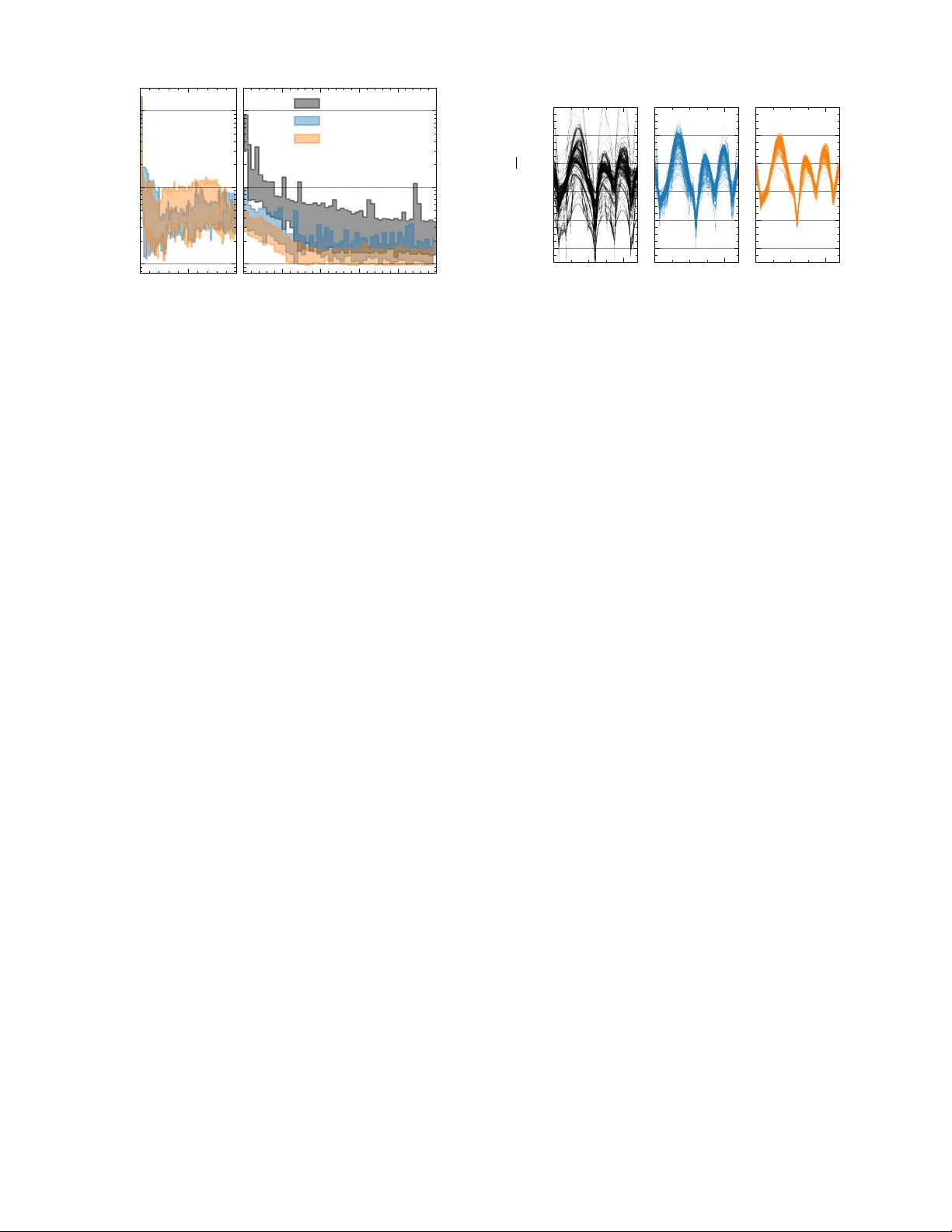
Efficient Contr oller Learning fr om Human Pr efer ences and Numerical Data via Multi-Modal Surr ogate Models Lukas Theiner 1 , Maik Pfef ferkorn 1 , Y ongpeng Zhao 1 , 2 , Sebastian Hirt 1 and Rolf Findeisen 1 Abstract — T uning control policies manually to meet high- level objectives is often time-consuming. Bayesian optimization pro vides a data-efficient framework for automating this process using numerical evaluations of an objective function. However , many systems — particularly those in volving humans — requir e optimization based on subjecti ve criteria. Pr eferential Bayesian optimization addresses this by learning from pairwise comparisons instead of quantitative measurements, but relying solely on prefer ence data can be inefficient. W e propose a multi-fidelity , multi-modal Bayesian optimization framework that integrates low-fidelity numerical data with high-fidelity human prefer ences. Our approach employs Gaussian process surrogate models with both hierarchical, autor egressi ve and non-hierarchical, cor egionalization-based structures, enabling efficient lear ning fr om mixed-modality data. W e illustrate the framework by tuning an autonomous vehicle’s trajectory planner , showing that combining numerical and pr eference data significantly reduces the need for experiments in volving the human decision maker while effectively adapting driving style to individual preferences. ©2026 IEEE. Personal use of this material is permitted. Permission from IEEE must be obtained for all other uses, including reprinting/republishing this material for advertising or promotional purposes, collecting new collected works for resale or redistribution to servers or lists, or reuse of any copyrighted component of this work in other works. I . I N T RO D U C T I O N Control policies, deriv ed from either traditional methods or optimization-based approaches such as model predictiv e control (MPC), often require tuning to meet higher-le vel objectiv es. This tuning process is often performed manually by experts, which can be time-consuming, costly , and error- prone. More recently , there has been a growing interest in methods that automate the learning of controller parameters to optimize closed-loop performance [1], [2], [3], [4], [5], [6], [7]. While v arious approaches hav e been proposed to address this challenge, Bayesian optimization (BO) [8] has gained particular attention, especially in settings where data collection is expensi ve or limited. BO offers a data-ef ficient, black-box optimization framework that operates on a user- defined higher -level objectiv e function and employs data- driv en surrogate models, typically Gaussian processes (GPs) [9], to guide the search for optimal controller parameters. In doing so, it can significantly reduce the number of costly closed-loop experiments required while effecti vely improving control performance. In some applications, howe ver , defining a suitable objec- tiv e function for the higher-le vel goal is not straightforward. This challenge arises particularly in systems that directly interact with humans, where the user’ s subjective percep- tion becomes the decisiv e performance criterion. Examples 1 Control and Cyber -Physical Systems Laboratory , T echnical Univer - sity of Darmstadt, Darmstadt, Germany , { rolf.findeisen, lukas.theiner, maik.pfefferk orn, sebastian.hirt } @iat.tu-darmstadt.de 2 V olkswagen A G, W olfsbur g, Germany , yongpeng.zhao@volkswagen.de This work was supported by V olkswagen AG. include assistiv e devices such as exoskeletons and rehabil- itation robots [10], collaborativ e robotic systems [11], and automated dri ving applications [12], [13]. For such cases, preferential Bayesian optimization (PBO) [14] provides a promising alternative. PBO e xtends classical Bayesian op- timization by constructing its surrogate model not from quantitativ e e valuations of an objectiv e function, but from qualitativ e user feedback in the form of pairwise prefer- ence comparisons [15], [16]. This allows optimization to be guided by subjectiv e assessments of performance, making it particularly suitable for scenarios inv olving humans. Howe ver , learning controller parameters solely from pref- erence data can be inef ficient in practice, since each prefer- ence query con veys much less information than a numerical ev aluation. Consequently , a large number of closed-loop experiments with a human decision maker may be required, especially in high-dimensional parameter spaces. Moti vated by these challenges, we generalize and extend pre vious approaches by proposing a systematic framework for using multiple information sources, including those that provide preferential feedback. Classical Bayesian optimization methods, which rely ex- clusiv ely on numerical ev aluations of the objective function, hav e been extensi vely studied in the context of multiple in- formation sources [17], [18], [19], [20]. A common category of these methods is multi-fidelity approaches, in which one or more lower -fidelity sources are av ailable alongside the main objective function. Such sources are typically cheaper to ev aluate but provide only an approximate assessment of the objectiv e. These settings arise frequently , for example, when a costly real-world experiment can be supplemented by a cheaper simulation that does not perfectly match real-world conditions. F or instance, a hierarchical GP surrogate model structure was employed in [21], [22] to combine simulation and real-world data for vehicle controller tuning. Similarly , policy tuning for robotic systems using both simulation and experimental data has been inv estigated in [23], where, how- ev er, the GP surrogate model does not impose a hierarchical relationship between the sources. Several other multi-fidelity Bayesian optimization methods hav e been adapted to address settings where auxiliary information sources exhibit varying or poor quality [24], [25], [26]. In this w ork, we build on established multi-fidelity ap- proaches by considering hierarchical and non-hierarchical surrogate model structures that incorporate multiple informa- tion sources. Our framew ork extends classical multi-fidelity optimization to scenarios where the av ailable sources dif fer not only in fidelity but also in modality , including those that pro vide preferential feedback rather than numerical ev aluations. Specifically , we develop multi-modal GP models to inte grate numerical and preferential data. These models are based on both hierarchical, autoregressi ve structures and non- hierarchical, coregionalization-based structures. W e discuss computational aspects related to model training and inference and describe their application within BO to optimize higher- lev el objectives using both numerical and preferential data. Finally , we demonstrate our proposed approach in the context of tuning a trajectory planner for autonomous driving. In this setting, numerical data act as lo w-fidelity information, deriv ed from a fix ed-structure, approximate performance measure, while preferential data serve as high-fidelity infor- mation, obtained directly from human drivers or passengers. The remainder of this article is organized as follows. In Section II, we formalize the considered setting. Section III introduces Gaussian process models based on numerical or preferential data and pro vides an overvie w of classical multi-fidelity model structures, along with a brief introduc- tion to Bayesian optimization. In Section IV, we propose multi-fidelity GP models that integrate both numerical and preferential data for use in PBO. Section V presents an application of the proposed models to trajectory planning for autonomous driving within the PBO framew ork. Finally , we conclude in Section VI. I I . P RO B L E M F O R M U L A T I O N W e consider a controlled dynamical system x t +1 = f  x t , u t ) , u t = π ξ ( x t ) (1) with state x t ∈ X ⊂ R n x , input u t ∈ U ⊂ R n u , and time index t ∈ N . The system dynamics are described by a function f : X × U → X , and the system is controlled by a parameterized policy π ξ : X → U , where ξ ∈ I ⊂ R n ξ denotes the adjustable parameters. Applying the control polic y π ξ in the closed loop for T ∈ N steps from an initial state x 0 generates a closed-loop trajectory τ ( ξ , x 0 ) = ( { x t } t ∈ [0 ,...,T ] , { u t } t ∈ [0 ,...,T − 1] ) . The dynamical system interacts with a human decision maker , who e valuates the performance of the closed-loop trajectory τ ( ξ, x 0 ) for a giv en parameter set ξ according to a latent, unknown objective function G : R n ξ → R , ξ 7→ G ( ξ ) . (2) The goal is to identify parameters ξ that optimize this latent objectiv e function, which reflects the decision maker’ s preferences. T o this end, the decision maker can be queried to express pairwise preferences between two parameter con- figurations ( ξ a , ξ b ) after observing the corresponding system behaviors. Since each query requires a physical experiment in volving the human, the total number of queries is limited by the experimental budget, making data-efficient learning of the optimal parameters essential. T o improv e data efficienc y , an additional information source ˆ G : R n ξ → R , ξ 7→ ˆ G ( ξ ) (3) is assumed to be a vailable. This may include, for e xample, a simulation model of the controlled dynamical system (1) f ( x t , u t ) π ξ ( x t ) x t u t High-fidelity Experiment f ( x t , u t ) π ξ ( x t ) x t u t Low-fidelity Simulation  ˆ G τ ( ξ , x 0 ) ˆ τ ( ξ , x 0 ) Multi-Modal Multi-Fidelity Bayesian Optimization ξ a , ξ b ξ m l ˆ G ( ξ ) Fig. 1. Structure of the proposed multi-modal multi-fidelity BO framework. Due to the human decision maker, the high-fidelity experiment only returns preferential data. The additional information source provides low-fidelity numerical e valuations. and an approximation of the decision maker’ s ev aluation process (2). While system models are commonly av ailable in control design, modeling the decision maker depends on the application context and may reflect characteristic human behavior or f actors such as comfort, cogniti ve effort, or perceiv ed safety , based on simulated or measured quantities. T o improve data efficienc y , the outputs of the additional information source (3) are assumed to be correlated with the original objectiv e function (2). The approach presented herein generalizes naturally to multiple additional information sources; for simplicity of presentation, we restrict the analysis to one such source. The considered setting is visualized in Figure 1. I I I . G AU S S I A N P R O C E S S E S & B A Y E S I A N O P T I M I Z A T I O N T o optimize the high-level objective, we employ Bayesian optimization, which utilizes a surrogate model of the objec- tiv e function — commonly a Gaussian process. This section therefore outlines the fundamentals of Gaussian process modeling, covering both the standard regression setting and the case where a latent function is inferred solely from preferential observations. In addition, we summarize two established approaches for constructing Gaussian process models that inte grate multiple numerical information sources, and conclude with a brief o vervie w of Bayesian optimization. A. Basics of Gaussian Process Re gr ession Gaussian processes generalize the concept of Gaussian random vectors to infinite-dimensional function spaces and are commonly interpreted as Gaussian probability distribu- tions over functions. Formally , a GP is denoted by g ( ξ ) ∼ G P ( m θ ( ξ ) , k θ ( ξ , ξ ′ )) , (4) and defines a collection of random variables { g ( ξ ) | ξ ∈ I ⊆ R n ξ } , indexed by ξ , any finite number of which are jointly Gaussian distributed [9]. A Gaussian process model is fully defined by the prior mean function m θ : R n ξ → R , ξ 7→ E [ g ( ξ )] and the prior cov ariance function k θ : R n ξ × R n ξ → R , ( ξ , ξ ′ ) 7→ C ov [ g ( ξ ) , g ( ξ ′ )] , which both depend on a set of hyperparameters θ . Giv en fixed hyperparameters θ , ev aluating (4) at a finite set of inputs ( ξ 1 , . . . , ξ d ) yields a multiv ariate Gaussian distribution ( g ( ξ 1 ) , . . . , g ( ξ d )) ∼ N ( µ, Σ) with mean vector µ , with entries [ µ ] i = m θ ( ξ i ) , and covariance matrix Σ , with entries [Σ] ij = k θ ( ξ i , ξ j ) . In the context of Bayesian optimization, Gaussian pro- cesses are commonly used as surrogate models of the un- known objecti ve function. More generally , Gaussian pro- cesses are used to probabilistically model an unknown function G ( ξ ) : R n ξ → R based on a finite set of prior observations. Specifically , we rely on a data set D = (Ξ , O ) , where Ξ ∈ R n Ξ × n ξ is the input matrix with rows [Ξ] i : = ξ ⊤ i and O denotes corresponding observations related to the function. Notably , the nature of O depends on whether the Gaussian process model g of G is constructed from numer- ical or preferential data; this distinction will be elaborated upon shortly . The objective is to le verage the av ailable data together with the prior model introduced in (4) to make informed predictions of the unobserved function values g ∗ = [ G ( ξ ∗ , 1 ) , . . . , G ( ξ ∗ ,n ∗ )] ⊤ at test locations Ξ ∗ , [Ξ ∗ ] i : = ξ ⊤ ∗ ,i , which are jointly distrib uted with the latent function values g = [ G ( ξ 1 ) , . . . , G ( ξ n Ξ )] ⊤ at training inputs Ξ . T o this end, gi ven a data set D of observ ations of the underlying function G , we aim to infer the data-informed posterior distribution p ( g ∗ | D , Ξ ∗ ) . T o achie ve this, we consider the conditional Gaussian distribution g ∗ | Ξ , g , Ξ ∗ , θ ∼ N ( µ g ∗ | g , Σ g ∗ | g ) , where (5) µ g ∗ | g = m θ (Ξ ∗ ) + k θ (Ξ ∗ , Ξ) k θ (Ξ , Ξ) − 1 ( g − m θ (Ξ)) , Σ g ∗ | g = k θ (Ξ ∗ , Ξ ∗ ) − k θ (Ξ ∗ , Ξ) k θ (Ξ , Ξ) − 1 k θ (Ξ , Ξ ∗ ) . Here, m θ ( A ) denotes the vector with entries [ m θ ] i = m θ ([ A ] i : ) , and k θ ( A, B ) denotes the cov ariance matrix with entries [ k θ ( A, B )] ij = k θ ([ A ] ⊤ i : , [ B ] ⊤ j : ) for A, B ∈ { Ξ , Ξ ∗ } . W e further consider the likelihood p ( O | g , θ ) , which quantifies the probability of observations O gi ven the latent function values g under a Gaussian process model with hyperparameters θ . In general, the hyperparameters may also be treated as uncertain, with a prior distribution θ ∼ p ( θ ) . Applying Bayes’ theorem, the posterior model is giv en by p ( g ∗ | D , Ξ ∗ ) ∝ Z Z p ( g ∗ | Ξ , g , Ξ ∗ , θ ) p ( O | g , θ ) p ( g | Ξ , θ ) p ( θ ) d g d θ . (6) The mean of the posterior distribution (6) provides an esti- mate of the unkno wn function values G ( ξ ∗ , 1 ) , . . . , G ( ξ ∗ ,n ∗ ) , while its (co-)variance quantifies the associated prediction uncertainty . 1) Numerical observations: In many settings, Gaussian process models are trained on numerical data. In such cases, the observations O are the target vector y consisting of noisy e valuations of the underlying function, i.e., [ y ] i = G ( ξ i ) + ε i , where the noise terms ε i are typically assumed to be independent and identically distributed Gaussian random variables, ε i ∼ N (0 , σ 2 n ) , with zero mean and v ariance σ 2 n . This assumption implies a Gaussian likelihood p ( O | g , θ ) . Moreov er , in most applications, a point estimate θ ∗ , ob- tained, e.g., via evidence maximization or cross-validation, is typically used [9]. Combined with the Gaussian likelihood assumption, this leads to a posterior p ( g ∗ | D , Ξ ∗ , θ ∗ ) that is itself Gaussian and can be expressed in closed-form g ∗ | D , Ξ ∗ , θ ∗ ∼ N ( m + θ ∗ (Ξ ∗ ) , k + θ ∗ (Ξ ∗ , Ξ ∗ )) , where m + θ ∗ (Ξ ∗ ) = m θ ∗ (Ξ ∗ ) + k θ ∗ (Ξ ∗ , Ξ)Σ − 1 y ( y − m θ ∗ (Ξ)) , k + θ ∗ (Ξ ∗ , Ξ ∗ ) = k θ ∗ (Ξ ∗ , Ξ ∗ ) − k θ ∗ (Ξ ∗ , Ξ)Σ − 1 y k θ ∗ (Ξ , Ξ ∗ ) , with Σ y = k θ ∗ (Ξ , Ξ) + σ 2 n I denoting the cov ariance matrix of the observations y . In settings with non-Gaussian noise or uncertain hyperpa- rameters θ ∼ p ( θ ) , approximations are typically required to obtain a closed-form posterior [9], or alternati vely , the pos- terior can be estimated directly using Markov-chain Monte- Carlo (MCMC) methods to e valuate either the fully Bayesian posterior p ( g ∗ | D , Ξ ∗ ) in (6) or the conditional posterior p ( g ∗ | D , Ξ ∗ , θ ∗ ) , depending on whether a fixed or marginal treatment of hyperparameters is adopted. 2) Prefer ence observations: In preference learning with Gaussian processes [15], the latent function is modeled based on preference observ ations in the form of pairwise comparisons. Instead of noisy ev aluations of the underlying function, the observ ations O are in the form of a set of n C comparisons C = { ( i k , j k ) | k ∈ { 1 , . . . , n C }} , where i k , j k ∈ { 1 , . . . , n Ξ } and i k  = j k . W ithin the set C , each tuple ( i k , j k ) represents one comparati ve judgment by the decision maker . In particular , the k th tuple ( i k , j k ) means that the decision maker preferred ξ i k ov er ξ j k . A common modeling assumption is that comparisons are based on the value of a latent objecti ve function, contaminated with Gaussian noise. This implies the so-called pr obit likelihood function p (( i, j ) | g ( ξ i ) , g ( ξ j )) = Z Z 1 { g ( ξ i )+ ε i ≥ g ( ξ j )+ ε j } ( ε i , ε j ) p ( ε i ) p ( ε j ) d ε i d ε j , where 1 A denotes the indicator function for the set A and ε i , ε j are independent and identically distributed ran- dom variables ε i , ε j ∼ N (0 , σ 2 n ) . Hence, the distrib ution p (( i, j ) | g ( ξ i ) , g ( ξ j )) admits the closed-form expression p (( i, j ) | g ( ξ i ) , g ( ξ j )) = Φ g ( ξ i ) − g ( ξ j ) p 2 σ 2 n ! , (7) where Φ is the cumulati ve distribution function of the standard normal distribution. Notably , unlike with numerical observations, the posterior distribution for preferential data is not Gaussian, even if the hyperparameters are known. It can either be approximated as Gaussian using the Laplace approximation [15], [9] or estimated via sampling-based approaches, such as MCMC methods. T o obtain a sampling-based approximation of the posterior (6), we first generate S posterior samples of the latent function v alues at training locations and hyperparameters, ( g ( s ) , θ ( s ) ) ∼ p ( g , θ | D ) , for s = 1 , . . . , S . Next, for each sample, we compute the conditional distri- bution of the test point, g ∗ | Ξ , g ( s ) , ξ ∗ , θ ( s ) , as defined in (5). Finally , resampling from these conditional distributions yields posterior predictiv e samples of g ∗ . B. Multi-F idelity Gaussian Pr ocesses T raditional Gaussian process regression, as discussed ear- lier , is designed to model data from a single, typically high- fidelity , source and assumes that all observations are of consistent quality . Howe ver , in many practical applications, acquiring high-fidelity data, such as through physical exper- iments or real-world testing, can be costly , time-intensiv e, or constrained by logistical limitations. T o mitigate the reliance on e xpensive data, lo w-fidelity simulations are often employed as a complementary , less resource-intensiv e alternativ e. This introduces the challenge of integrating heterogeneous data sources with differing lev- els of fidelity , which has led to the dev elopment of extended GP regression frame works for multi-fidelity settings [27]. In the following, we provide a concise summary of two established strategies to model multiple data sources G h ( ξ ) , h ∈ { 1 , . . . , H } through a collection of GPs g h ( ξ ) , h ∈ { 1 , . . . , H } . Importantly , these methods impose a correlation between the GP models, allo wing for information transfer between them. 1) Intrinsic Cor egionalization Model (ICM): A common approach to constructing surrogate models that integrate multiple information sources is the use of cor e gionalization [28], [20], as also emplo yed in multi-output Gaussian process regression [29]. In this framew ork, each information source is modeled as a separate but correlated Gaussian process g h , where dependencies are induced through a shared set of H latent Gaussian processes, u i ( ξ ) ∼ G P  m ( ξ ) , k ( ξ , ξ ′ )  , i ∈ { 1 , . . . , H } , that all share a common kernel function k b ut are mutually independent. Each model g h is a linear combination of the latent processes, g h ( ξ ) = H X i =1 a h,i u i ( ξ ) , h ∈ { 1 , . . . , H } , with coefficients a h,i ∈ R that determine how strongly output h depends on latent process i . Using the mutual independence of the latent GPs, the prior cross-cov ariance between g h and g h ′ can be deriv ed as C o v [ g h ( ξ ) , g h ′ ( ξ ′ )] = H X i =1 a h,i a h ′ ,i k ( ξ , ξ ′ ) = [ B ] hh ′ k ( ξ , ξ ′ ) , where the core gionalization matrix B = AA ⊤ has entries [ A ] hi = a h,i . This symmetric positiv e semi-definite matrix captures the inter-output correlations induced by the latent mixing structure, and its entries are inferred jointly with the kernel hyperparameters [20]. The ICM can equiv alently be viewed as a standard Gaus- sian process defined ov er an augmented input space ˜ I = I × { 1 , . . . , H } , with the corresponding augmented kernel ˜ k  ( ξ , h ) , ( ξ ′ , h ′ )  = [ B ] hh ′ k ( ξ , ξ ′ ) . (8) Inference in this formulation proceeds analogously to the single-output GP described in Section III-A.1. 2) Autor e gr essive Model (AR1): Secondly , we also utilize the autoregressiv e (AR1) model introduced in [17], which establishes a Gaussian process prior for each fidelity lev el and models their interdependencies through a recursive, linear structure. Let G h ( ξ ) , h = 1 , . . . , H represent a sequence of models of G with increasing fidelity . Each model’ s output is captured by a separate GP g h , defined analogously to (4). Specifically , at the base fidelity lev el h = 1 (lo west fidelity), we define a standard Gaussian process model g 1 ( ξ ) ∼ G P  m 1 ( ξ ) , k 1 ( ξ , ξ ′ )  . For subsequent fidelity le vels h = 2 , . . . , H , the model is recursiv ely defined via  g h ( ξ ) = ρ h − 1 g h − 1 ( ξ ) + δ h ( ξ ) , g h − 1 ( ξ ) ⊥ δ h ( ξ ) , (9) where the correction term δ h is itself modeled as an indepen- dent ( ⊥ ) Gaussian process δ h ( ξ ) ∼ G P  m δ h ( ξ ) , k δ h ( ξ , ξ ′ )  . In this formulation, the parameters ρ h − 1 gov ern the linear dependence between successive fidelity le vels. Due to the closure of Gaussian processes under linear transformations, the additiv e form in (9) ensures that all higher fidelity models g h , h = 2 , . . . , H , are themselves Gaussian processes. As in the single-fidelity case (Section III-A.1), closed- form posteriors are possible under Gaussian noise and fixed hyperparameters, whereas non-Gaussian noise or uncertain hyperparameters necessitate approximation or MCMC-based Bayesian inference. C. Bayesian Optimization W e apply Bayesian optimization to address the optimiza- tion problem ξ ∗ = arg min ξ ∈I G ( ξ ) , where G : R n ξ → R , ξ 7→ G ( ξ ) is a black-box function and ξ ∗ denotes its global minimizer within the feasible set I . Unlike classical optimization methods that require dense e valuations of the objectiv e, BO seeks to minimize the number of function ev aluations by sequentially selecting the most informative sampling points. This is particularly advan- tageous when the true objecti ve G is unkno wn and expensi ve to ev aluate. T o this end, BO relies on surrogate models of the objectiv e G — most commonly Gaussian processes — which are updated iterativ ely as new observations are gathered. Specifically , in each iteration n ∈ N , BO proceeds in two main steps: 1) Select a query point ξ n and ev aluate the objective function — which in the controller tuning case in volv es running a closed-loop experiment — to obtain a new data tuple ( ξ n , G ( ξ n )) , and 2) update the GP surrogate, including hyperparameters, using the augmented data set D n +1 = (Ξ n +1 , y n +1 ) , where Ξ n +1 ← [Ξ ⊤ n , ξ n ] ⊤ and y n +1 ← [ y ⊤ n , G ( ξ n )] ⊤ . For Preferential Bayesian optimization (PBO), with observa- tions in the form of pairwise comparisons, the steps are: 1) Select a pair of query points ( ξ i n , ξ j n ) and query the decision maker — by running two closed-loop exper- iments — to obtain a new data tuple ( ξ i n , ξ j n , c n ) , where c n = ( i n , j n ) if ξ i n is preferred over ξ j n and c n = ( j n , i n ) otherwise, and 2) update the GP surrogate, including hyperparameters, using the augmented data set D n +1 = (Ξ n +1 , C n +1 ) , where Ξ n +1 ← [Ξ ⊤ n , ξ i n , ξ j n ] ⊤ and C n +1 ← C n ∪ { c n } . T o steer the selection of the query points ξ n tow ard the global minimizer ξ ∗ , BO relies on an acquisition function α BO . This function uses the current GP surrogate for G to quantify the utility of e valuating a candidate point, effecti vely balancing exploration of uncertain regions with e xploitation of promising areas. At each iteration n , the next point to ev aluate is selected by maximizing this acquisition function: ξ n = arg max ξ ∈I α BO ( ξ ; D n ) , where α BO : R n ξ → R , ξ 7→ α BO ( ξ ; D n ) . For an overvie w of commonly used acquisition functions in the standard setting with numerical observations, we refer the reader to [8]. In preferential Bayesian optimization, a pair of points for the next comparison is selected instead: ( ξ i n , ξ j n ) = arg max ( ξ,ξ ′ ) ∈I 2 α PBO ( ξ , ξ ′ ; D n ) , where α PBO : R n ξ × R n ξ → R , ( ξ , ξ ′ ) 7→ α PBO ( ξ , ξ ′ ; D n ) . A widely used pairwise acquisition function is the expected utility of the best option (EUBO) [30], [31]. For a summary of alternative acquisition functions in the preferential setting, see [31] and the references therein. D. Multi-F idelity Bayesian Optimization In multi-fidelity Bayesian optimization, a surrogate model incorporating data from all information sources is used to improv e data ef ficiency with respect to the main, high-fidelity source. Depending on the application context, two distinct strategies can be employed. The first strategy employs cost- aware acquisition functions to dynamically select the most informativ e and cost-ef fectiv e fidelity at each iteration [18], [20], [24]. The second strategy organizes the optimization into distinct phases, starting with exploration on low-fidelity data and transitioning to high-fidelity ev aluations in later stages [21], [22]. In this phased approach, e xploration- oriented acquisition functions — such as the inte gral pre- dictive variance (IPV) [32] — should be used during the low-fidelity phase, as demonstrated by [21]. I V . M U LT I - M O DA L M U LT I - F I D E L I T Y S U R R O G A T E S C O M B I N I N G P R E F E R E N T I A L A N D N U M E R I C A L D AT A Multi-fidelity methods for Bayesian optimization aim to reduce the reliance on e xpensiv e data by utilizing addi- tional lower-fidelity data sources. Prior work was limited to combining data sources providing numerical ev aluations of the objecti ve function. In this section, we extend these approaches by integrating both numerical and preferential observations of different fidelities into a unified multi-modal, multi-fidelity surrogate model. For clarity of exposition, the following discussion considers two fidelity lev els ( H = 2 ), without loss of generality . Specifically , the high-fidelity lev el ( h = 2 ) corresponds to pairwise comparisons of (2) and is denoted by superscript hf . The low-fidelity level ( h = 1 ) corresponds to numerical observations of (3) and is denoted by superscript lf . As discussed earlier , this setting captures scenarios in which controller or system parameters are learned according to human preferences, while an av ail- able system model and approximate, numerically tractable decision criterion are leveraged to minimize the need for human-in volved experiments. A. Multi-Modal ICM Surr ogates W e begin by discussing the implications of incorporating multi-modal data for the application of the ICM (cf. Section III-B.1) as a multi-fidelity surrogate. For clarity of expo- sition, we treat the ICM as a standard GP ˜ g defined ov er an augmented input space and equipped with an augmented kernel ˜ k , as in (8). The problem thus reduces to conditioning a GP simultaneously on numerical and preference observa- tions. W e denote the augmented high-fidelity and low-fidelity in- puts by ˜ ξ hf i = ( ξ hf i , 1) and ˜ ξ lf i = ( ξ lf i , 2) , respectively . Assum- ing conditional independence of all observations giv en the latent function values ˜ g = [( ˜ g hf ) ⊤ , ( ˜ g lf ) ⊤ ] ⊤ , where ˜ g hf = [ ˜ g ( ˜ ξ hf 1 ) , . . . , ˜ g ( ˜ ξ hf n Ξ , hf )] ⊤ and ˜ g lf = [ ˜ g ( ˜ ξ lf 1 ) , . . . , ˜ g ( ˜ ξ lf n Ξ , lf )] ⊤ , the joint likelihood factorizes as p ( D | g ) = Y ( i,j ) ∈C hf Φ ˜ g ( ˜ ξ hf i ) − ˜ g ( ˜ ξ hf j ) p 2 σ 2 n ! · Y ( ξ lf i ,y lf i ) ∈D lf N  y lf i ; ˜ g ( ˜ ξ lf i ) , σ 2 n  , where preference observ ations are incorporated through the probit likelihood (7) and numerical observations through a Gaussian likelihood. As the joint likelihood is non-Gaussian, the posterior must be approximated, as in the single-fidelity preference GP case (Section III-A.2). Specifically , we em- ploy MCMC-based approximations. For the two-fidelity problem, we adopt the coregionaliza- tion matrix B =  σ 2 hf ρ σ hf σ lf ρ σ hf σ lf σ 2 lf  , where ρ ∈ [0 , 1) and σ hf , σ lf ∈ R + are h yperparameters. This ensures that B is positiv e definite. W e place a Beta( α, β ) prior on ρ with α > β , biasing the distribution toward v alues near 1 to promote information transfer from low to high fidelity when only low-fidelity data hav e been collected. B. Multi-Modal AR1 GP Surro gates In contrast to the intrinsic core gionalization approach, the AR1 scheme (cf. Section III-B.2) incorporates data of different modalities hierarchically through a two-step pro- cess. W e first condition a standard GP (4) on the numerical low-fidelity observations in the dataset D lf to obtain the low-fidelity model g lf ( ξ ) . Ne xt, we use the low-fidelity GP model to predict the mean and variance at the inputs Ξ hf , where high-fidelity comparati ve ev aluations were performed. For sampling-based inference via MCMC methods, these predicted statistics are computed empirically . The high-fidelity model, which inte grates both numerical and preferential data, is then e xpressed as g hf ( ξ ) = g lf ( ξ ) + δ ( ξ ) , where δ is a preference-based GP , and, in contrast to (9), we omit the scaling parameter ρ . This omission is justified because the scale of g hf is negligible when conditioned only on comparativ e data, making ρ redundant with the scaling parameter of the δ -GP kernel. It remains to infer the h yperparameters of the δ -GP , as well as the vector of latent values δ , where [ δ ] i = δ ( ξ hf i ) , i = 1 , . . . , n hf Ξ using MCMC sampling from the joint posterior p ( δ , θ | D hf ) ∝ p ( D hf | δ , θ ) p ( δ | θ ) p ( θ ) , where p ( θ ) is the prior over hyperparameters, p ( δ | θ ) is the zero-mean GP prior, and p ( D hf | δ , θ ) is the likelihood of the observed preference relations in D hf . The likelihood for each comparison c = ( i, j ) ∈ C hf is computed as p ( c | δ ( ξ hf i ) , δ ( ξ hf j )) = Z Z Z 1 { g lf ( ξ hf i )+ δ ( ξ hf i )+ ε i ≥ g lf ( ξ hf j )+ δ ( ξ hf j )+ ε j } ( ε i , ε j , g lf ) p  g lf ( ξ hf i ) , g lf ( ξ hf j )  p ( ε i ) p ( ε j ) d ε i d ε j d g lf , (11) where ε i , ε j ∼ N (0 , σ 2 n ) represent independent additi ve noise accounting for inconsistencies in human decisions, and σ n is a hyperparameter of the model. By introducing η = g lf ( ξ hf j ) − g lf ( ξ hf i ) + ε j − ε i with η ∼ N ( E  g lf ( ξ hf j )  − E  g lf ( ξ hf i )  , C ov  g lf ( ξ hf j ) − g lf ( ξ hf i )  + 2 σ 2 n ) , (11) simpli- fies to p ( c | δ ( ξ hf i ) , δ ( ξ hf j )) = Z 1 { δ ( ξ hf i ) − δ ( ξ hf j ) ≥ η } ( η ) p ( η ) d η = Φ   δ ( ξ hf i ) + E  g lf ( ξ hf i )  − δ ( ξ hf j ) − E  g lf ( ξ hf j )  q C o v  g lf ( ξ hf j ) − g lf ( ξ hf i )  + 2 σ 2 n )   , where Φ , as pre viously , denotes the cumulati ve distribution function of the standard normal distrib ution. Finally , we compute the posterior distribution under the multi-modal AR1 model using MCMC methods, as described in Section III-A.2. 0 1000 2000 Path progress (m) 40 60 80 100 V elocity ( km h ) − 250 0 250 East (m) 0 200 400 600 800 1000 North (m) Fig. 2. Left: Black and green areas sho w the 2 σ credible intervals of the heteroscedastic Gaussian processes modeling observed human driver trajectories. The black model, trained on a range of drivers, serves as a low-fidelity model, while the green model, trained on one driver , is utilized to simulate high-fidelity preferences of a passenger for method ev aluation. In each comparison, the simulated passenger prefers the trajectory that better aligns with the green model. Right: Overview of the track layout. V . E X A M P L E : P E R S O N A L I Z E D A UT O M A T E D D R I V I N G While automated driving systems can be designed mainly based on clearly defined, numerically tractable objectiv es — such as minimizing trav el time, reducing energy con- sumption, or maintaining desired safe distances from other vehicles — they often must also account for more subjectiv e goals, including passenger comfort [33], perceived safety , or driving style. In this w ork, we focus on the task of tuning an au- tomated driving system according to individual passenger preferences, b uilding on our previous study [13]. The system employs an optimization-based trajectory planner followed by a trajectory tracking controller . At each planning stage k , the planned trajectory ˆ τ ∗ k is obtained as the solution of an optimal control problem. For details regarding the vehicle model and the formulation of the optimal control problem, we refer the reader to [13]. T o adapt the dri ving style to individual preferences, we learn parameters of the trajectory planner — specifically , the weights of the cost function of the underlying optimal control problem — using multi-modal multi-fidelity BO, as illustrated in Figure 1. In particular, we optimize the weights associated with positiv e and negati ve longitudinal accelera- tion, lateral acceleration, longitudinal jerk, and lateral jerk, resulting in n ξ = 5 parameters. T o facilitate sample-efficient learning, we construct a low-fidelity model of the human decision-making process from observed trajectories of human dri vers. Specifically , we proceed as in our previous work [13], and model the range of observed velocity profiles using a heteroscedastic GP [34], see the black shaded area in Figure 2. The resulting lo w- fidelity model of the human decision-making process is then expressed as the likelihood of a simulated trajectory under this probabilistic model. This low-fidelity model provides a numerical approximation of human preferences, which can be combined with high-fidelity preferential feedback in the proposed multi-modal multi-fidelity BO framework. 0 50 Low-fidelity episodes 10 3 10 4 10 5 Regret 0 10 20 30 40 50 High-fidelity episodes PBO MM-MFBO (ICM) MM-MFBO (AR1) Fig. 3. Regret of the recommended parameters ξ ∗ n — obtained by maximizing the posterior mean of the surrogate model — after each episode of the BO procedure. Shaded areas show the total range observed over fiv e trials. Regret is computed using the true objectiv e function G ( ξ ) underlying the preferences of the simulated passenger . In the follo wing, we e v aluate our method using a simulated passenger , where the true objective function underlying their preferences is known. This is necessary for a quantitativ e ev aluation using regret as a performance measure. Regret plots cannot be generated in realistic settings, where the true objectiv e guiding the preferences is unkno wn. High-fidelity preferential feedback is modeled using a heteroscedastic GP trained on a distinct set of trajectories from a single dri ver , as indicated by the green shaded area in Figure 2. T o ev aluate our proposed multi-modal multi-fidelity sur- rogates, we compare (i) standard preferential BO using a preferential GP surrogate model (cf. Section III-A.2), (ii) multi-modal multi-fidelity BO based on the proposed multi- modal ICM surrogate (cf. Section IV -A), and (iii) multi- modal multi-fidelity BO based on the proposed multi-modal AR1 surrogate (cf. Section IV -B). For the multi-modal methods, the optimization is split into a low-fidelity phase, where numerical observations of the low-fidelity objectiv e are collected, and a high-fidelity phase, where the high- fidelity objecti ve is optimized based on preferential feedback. All three procedures use the expected utility of the best option (EUBO) acquisition function [31] to propose ne w comparison candidates during the high-fidelity phase. The multi-fidelity methods additionally employ the inte gral pre- dictive variance (IPV) acquisition function [32] during the first 80 episodes of the low-fidelity phase, followed by 20 episodes using expected impr ovement (EI) [8]. This choice is consistent with the strategy outlined in Section III-D, which in volves mainly using exploration-intensi ve acquisition func- tions during the low-fidelity phase. For all methods, posterior samples are dra wn using the Pyro [35] implementation of the NUTS algorithm [36], an extension of the Hamiltonian Monte Carlo (HMC) MCMC algorithm. Figure 3 shows the regret of the three procedures over the course of the optimization runs. Regret is computed as the difference in performance between the trajectory induced by the best parameter recommendation after each episode — obtained by maximizing the posterior mean of the surrogate 0 2000 20 40 60 80 100 120 V elocity ( km h ) PBO 0 2000 Path progress (m) MM-MFBO (ICM) 0 2000 MM-MFBO (AR1) Fig. 4. T rajectories sampled during the high-fidelity phases of each method, aggregated across all fiv e experimental trials. — and the best possible trajectory under the known objecti ve. Both proposed multi-fidelity methods clearly outperform the single-fidelity preferential Bayesian optimization, benefiting from successful information transfer from the preceding lo w- fidelity ev aluations. In fact, the single-fidelity baseline requires approximately 10 to 15 high-fidelity episodes to reach regret scores that the proposed multi-modal multi-fidelity models achieve solely with lo w-fidelity data, before observing a single high-fidelity preference. Since each high-fidelity episode corresponds to a pair of closed-loop experiments, this corresponds to 20 to 30 closed-loop experiments. In our ev aluation, the autoregressi ve (AR1) structure achiev es more consistent results and outperforms the ICM. W e conjecture that this is due to the simpler and hierarchical correlation structure of the AR1 model, which naturally aligns with our setting. In contrast, the correlation between fidelities in the ICM is more sensitiv e to v ariability in hyperparameter inference, which may lead to inconsistent performance across episodes. This arises from the fact that the ICM does not a priori assume a hierarchical relation between the data sources, but treats them on equal footing. The correlation structure must therefore be inferred from the data via hyperparameter estimation of the coregionalization matrix. While this provides greater fle xibility in modeling complex correlations compared to the AR1 model, accurately identifying the correlation structure from limited data can be challenging. Finally , a similar trend can be observed when comparing the parameters queried by each method in e very episode, rather than just the regret of the best recommendation ov er the episodes. W e emphasize that, in human-in volv ed con- troller tuning, performance across all sampled comparisons is important: the human decision maker may experience dis- comfort when ev aluating inferior parameterizations. Conse- quently , following our previous work [13], we also examine the trajectories resulting from the parameters sampled across all high-fidelity episodes. As sho wn in Figure 4, the results indicate that the multi-fidelity structure significantly focuses the preference queries and reduces frequent sampling of inferior parameters. V I . C O N C L U S I O N Efficiently tuning controllers based on human preferences requires integrating additional information sources to mini- mize costly human feedback. This work presents a frame- work for multi-modal, multi-fidelity Bayesian optimization that inte grates numerical and preferential data to enable efficient learning of controller parameters. Extending clas- sical multi-fidelity Gaussian process formulations, we pro- pose two surrogate model structures — a coregionalization- based model and a hierarchical autoregressiv e AR1 model — capable of jointly representing numerical e valuations and pairwise preference feedback. Both surrogate structures facilitate information transfer across fidelities and modalities, thereby substantially improving data efficiency in settings where high-fidelity human feedback is limited. The framew ork is demonstrated on a personalized auto- mated driving task, where controller parameters are adapted to individual passenger preferences. The results indicate that both multi-modal, multi-fidelity surrogate models outperform standard preference-only Bayesian optimization by achieving faster and more consistent adaptation of the driving style. Among the two approaches, the AR1 structure exhibits particularly robust performance, suggesting that hierarchical formulations of fer adv antages when combining heteroge- neous data modalities. Finally , although demonstrated in automated driving, the proposed framework is general in nature and directly appli- cable to a wide range of controller tuning tasks inv olving hu- man preferences, including exoskeletons, assistiv e robotics, autonomous driving, and other human-centered applications. R E F E R E N C E S [1] A. Marco, P . Hennig, J. Bohg, S. Schaal, and S. Trimpe, “ Automatic LQR tuning based on Gaussian process global optimization, ” in IEEE Int. Conf. Robot. and Autom. , 2016, pp. 270–277. [2] F . Berkenkamp, A. P . Schoellig, and A. Krause, “Safe controller optimization for quadrotors with Gaussian processes, ” in IEEE Int. Conf. Robot. and Autom. , 2016, pp. 491–496. [3] D. Piga, M. Forgione, S. Formentin, and A. Bemporad, “Performance- oriented model learning for data-driven MPC design, ” IEEE Control Syst. Lett. , vol. 3, no. 3, pp. 577–582, 2019. [4] S. Hirt, M. Pfefferkorn, A. Mesbah, and R. Findeisen, “Stability- informed Bayesian optimization for MPC cost function learning, ” IF A C-P apersOnLine , vol. 58, no. 18, pp. 208–213, 2024. [5] S. Hirt, M. Pfefferk orn, and R. Findeisen, “Safe and stable closed- loop learning for neural-network-supported model predictiv e control, ” in IEEE Conf. Decis. Contr ol , 2024, pp. 4764–4770. [6] P . Holzmann, M. Pfefferkorn, J. Peters, and R. Findeisen, “Learning energy-ef ficient trajectory planning for robotic manipulators using Bayesian optimization, ” in Eur . Control Conf. , 2024, pp. 1374–1379. [7] S. Hirt, L. Theiner, M. Pfefferk orn, and R. Findeisen, “ A hierarchical surrogate model for efficient multi-task parameter learning in closed- loop control, ” in IEEE Conf. Decis. Contr ol , 2025, pp. 4578–4585. [8] R. Garnett, Bayesian Optimization . Cambridge Univers. Press, 2023. [9] C. E. Rasmussen and C. K. I. Williams, Gaussian Processes for Machine Learning . MIT Press, 2006. [10] K. A. Ingraham, M. Tuck er , A. D. Ames, E. J. Rouse, and M. K. Shepherd, “Leveraging user preference in the design and ev aluation of lower -limb exoskeletons and prostheses, ” Curr . Opin. Biomed. Eng. , vol. 28, p. 100487, 2023. [11] L. Roveda, L. Mantov ani, M. Maccarini, F . Braghin, and D. Piga, “Optimal physical human–robot collaborative controller with user- centric tuning, ” Contr ol Eng. Pract. , v ol. 139, p. 105621, 2023. [12] M. Zhu, A. Bemporad, and D. Piga, “Preference-based MPC calibra- tion, ” in Eur . Contr ol Conf. , 2021, pp. 638–645. [13] L. Theiner, S. Hirt, A. Steinke, and R. Findeisen, “Exploiting prior knowledge in preferential learning of individualized autonomous ve- hicle dri ving styles, ” in Eur . Control Conf. , 2025, pp. 2217–2222. [14] J. Gonz ´ alez, Z. Dai, A. Damianou, and N. D. Lawrence, “Preferential Bayesian optimization, ” in Int. Conf. Mach. Learn. , 2017, pp. 1282– 1291. [15] W . Chu and Z. Ghahramani, “Preference learning with Gaussian processes, ” in Int. Conf. Mach. Learn. , 2005, pp. 137–144. [16] E. Brochu, N. d. Freitas, and A. Ghosh, “ Active preference learning with discrete choice data, ” in Adv . Neural Inf. Pr ocess. Syst. , vol. 20, 2007, pp. 409–416. [17] M. C. Kennedy and A. O’Hagan, “Predicting the output from a complex computer code when fast approximations are av ailable, ” Biometrika , vol. 87, no. 1, pp. 1–13, 2000. [18] M. Poloczek, J. W ang, and P . Frazier , “Multi-information source optimization, ” in Adv . Neural Inf. Pr ocess. Syst. , vol. 30, 2017. [19] A. I. J. Forrester , A. S ´ obester , and A. J. Keane, “Multi-fidelity optimization via surrogate modelling, ” Proc. R. Soc. A , vol. 463, pp. 3251–3269, 2007. [20] K. Swersky , J. Snoek, and R. P . Adams, “Multi-T ask Bayesian opti- mization, ” in Adv . Neural Inf. Pr ocess. Syst. , vol. 26, 2013. [21] Y . Zhao, M. Pfefferkorn, M. T empler, and R. Findeisen, “Efficient learning of vehicle controller parameters via multi-fidelity Bayesian optimization: From simulation to e xperiment, ” in IEEE Intell. V eh. Symp. , 2025, pp. 1697–1704. [22] Y . Zhao, M. Pfefferkorn, M. T empler , D. T ¨ opfer , and R. Findeisen, “Cautious learning of vehicle controller parameters via constrained multi-fidelity Bayesian optimization, ” in Eur . Control Conf. , 2026. [23] S. He, A. von Rohr, D. Baumann, J. Xiang, and S. Trimpe, “Simulation-aided policy tuning for black-box robot learning, ” IEEE T rans. Robot. , vol. 41, pp. 2533–2548, 2025. [24] M. Nobar, J. Keller , A. Forino, J. L ygeros, and A. Rupenyan, “Guided multi-fidelity Bayesian optimization for data-driven controller tuning with digital twins, ” IEEE Robot. Autom. Lett. , 2026, to be published. [25] M. Fan, B. Y oon, E. Dougherty , N. Urban, F . Alexander, R. Arr ´ oyav e, and X. Qian, “Multi-fidelity Bayesian optimization with multiple information sources of input-dependent fidelity , ” in Conf. Uncert. Artif. Intell. , 2024, pp. 1271–1293. [26] P . Mikkola, J. Martinelli, L. Filstroff, and S. Kaski, “Multi-fidelity Bayesian optimization with unreliable information sources, ” in Int. Conf. Artif. Intell. Stat. , 2023, pp. 7425–7454. [27] L. Brevault, M. Balesdent, and A. Hebbal, “Ov erview of Gaussian pro- cess based multi-fidelity techniques with variable relationship between fidelities, application to aerospace systems, ” Aerosp. Sci. T echnol. , vol. 107, p. 106339, 2020. [28] E. Bonilla, K. Chai, and C. W illiams, “Multi-task Gaussian process prediction, ” in Adv . Neural Inf. Process. Syst. , vol. 20, 2007, pp. 153– 160. [29] M. A. ´ Alvarez, L. Rosasco, and N. D. Lawrence, “Kernels for vector- valued functions: A re view , ” F ound. T r ends Mach. Learn. , vol. 4, no. 3, 2012. [30] Z. J. Lin, R. Astudillo, P . Frazier, and E. Bakshy , “Preference explo- ration for efficient Bayesian optimization with multiple outcomes, ” in Int. Conf. Artif. Intell. Stat. , 2022, pp. 4235–4258. [31] R. Astudillo, Z. J. Lin, E. Bakshy , and P . Frazier , “qEUBO: A decision- theoretic acquisition function for preferential Bayesian optimization, ” in Int. Conf. Artif. Intell. Stat. , 2023, pp. 1093–1114. [32] S. Seo, M. W allat, T . Graepel, and K. Obermayer, “Gaussian process regression: active data selection and test point rejection, ” in IEEE- INNS-ENNS Int. Joint Conf. Neural Networks , vol. 3, 2000, pp. 241– 246. [33] A. Steinke, “Optimizing motion comfort in automated driving: Motion sickness reduction and augmented trajectory planning, ” Ph.D. disser- tation, T echnische Universit ¨ at Darmstadt, Darmstadt, 2025. [34] K. K ersting, C. Plagemann, P . Pfaff, and W . Burgard, “Most likely heteroscedastic Gaussian process regression, ” in Int. Conf. Mac h. Learn. , 2007, pp. 393–400. [35] E. Bingham, J. P . Chen, M. Jankowiak, F . Obermeyer, N. Pradhan, T . Karaletsos, R. Singh, P . Szerlip, P . Horsfall, and N. D. Goodman, “Pyro: Deep univ ersal probabilistic programming, ” J. Mach. Learn. Res. , vol. 20, no. 28, pp. 1–6, 2019. [36] M. D. Homan and A. Gelman, “The No-U-turn sampler: adaptiv ely setting path lengths in Hamiltonian Monte Carlo, ” J. Mach. Learn. Res. , vol. 15, no. 1, pp. 1593–1623, 2014.