Equivariant Filter Transformations for Consistent and Efficient Visual--Inertial Navigation

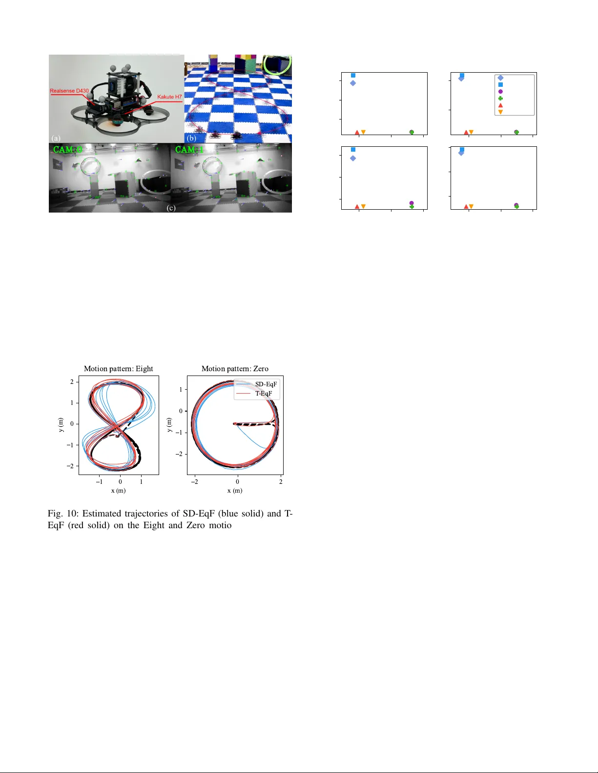
Equi v ariant Filter T ransformations for Consistent and Ef ﬁcient V isual–Inertial Na vigation Chungeng T ian, Fenghua He, and Ning Hao Abstract —This paper presents an equi variant ﬁlter (EqF) transformation approach for visual–inertial navigation. By estab- lishing analytical links between EqFs with different symmetries, the proposed appr oach enables systematic consistency design and efﬁcient implementation. First, we formalize the mapping from the global system state to the local error -state and prov e that it induces a nonsingular linear transformation between the error - states of any two EqFs. Second, we derive transformation laws for the associated linearized err or -state systems and unobserv able subspaces. These results yield a general consistency design principle: for any unobservable system, a consistent EqF with a state-independent unobservable subspace can be synthesized by transforming the local coordinate chart, thereby av oiding ad hoc symmetry analysis. Third, to mitigate the computational burden arising from the non-block-diagonal Jacobians required for consistency , we propose two efﬁcient implementation strate- gies. These strategies exploit the Jacobians of a simpler EqF with block-diagonal structure to accelerate covariance operations while pr eserving consistency . Extensive Monte Carlo simulations and real-world experiments validate the proposed appr oach in terms of both accuracy and runtime. Index T erms —Equivariant ﬁlter , visual–inertial navigation, estimation consistency , coordinate transformation. I . I N T RO D U C T I O N V ISU AL–Inertial Navigation Systems (VINS), which fuse high-frequency inertial measurements with visual ob- servations, have become a core technology for enabling au- tonomous robots to achie ve high-precision positioning in GPS- denied environments [ 1 ]–[ 6 ]. T o address the severe nonlinear- ities inherent in kinematic models, various ﬁlter-based nonlin- ear estimators have been developed. Among these, Equiv ariant Filter (EqF) [ 7 ]–[ 11 ] has received increasing attention in recent years. The core principle of EqF lies in exploiting inherent system symmetries to lift the nonlinear estimation problem from the original state manifold to an appropriate symmetry Lie group. This perspectiv e uniﬁes the design of classical VINS estimators [ 12 ], [ 13 ], such as the Error-State Kalman Filter (ESKF) [ 14 ]–[ 16 ] and the In variant Extended Kalman Filter (I-EKF) [ 17 ]–[ 21 ]. Furthermore, because EqF relies solely on fundamental equiv ariant properties rather than requiring the system model to be explicitly deﬁned on a Lie group, it is applicable to a broader range of complex systems, thereby signiﬁcantly extending its utility in the ﬁeld of state estimation. Despite the elegant theoretical uniﬁcation achiev ed by EqF , two critical problems remain unresolved. First, universal de- The authors are with School of Astronautics, Harbin Institute of T echnology , Harbin, 150000, China. (email: tcghit@outlook.com; hefenghua@hit.edu.cn; haoning@hit.edu.cn). Corresponding author: Fenghua He. sign criteria for consistent EqFs applicable to arbitrary un- observable systems are still lacking. Inconsistenc y typically arises when the unobservable subspace of a system depends on the state, causing estimators to become overconﬁdent in their uncertainty estimates along unobservable directions [ 22 ], [ 23 ]. Currently , two main approaches exist to ensure consistenc y: one inv olves modifying Jacobians to enforce observability constraints [ 22 ], [ 24 ], [ 25 ], which inevitably sacriﬁces Jaco- bian optimization; the other aims to attain a state-independent unobservable subspace [ 26 ], [ 27 ], a direction that is becoming a mainstream solution. While existing studies hav e achiev ed a state-independent subspace through the selection of appro- priate symmetries [ 7 ], [ 28 ], a systematic methodology for EqF remains absent. Consequently , identifying symmetries that ensure estimation consistency is still largely an empirical process, which presents substantial challenges for complex unobservable systems [ 29 ]. Second, a fundamental trade-off exists between theoretical consistency and computational ef ﬁciency in EqF . Speciﬁcally , the symmetries required for consistenc y often induce intri- cate differential geometric structures that disrupt the inher- ent block-diagonal structure of Jacobian matrices. In VINS, this manifests as a coupling between landmark and IMU pose errors within the propagation Jacobian, leading to a sharp increase in computational overhead. T o mitigate this, [ 30 ] combined I-EKF with the First-Estimates Jacobian (FEJ) methodology to decouple landmark uncertainty , albeit at the cost of optimality . More recently , [ 31 ] and [ 32 ] le veraged the block-diagonal structure of Error-State Kalman ﬁlters (ESKF) to enable efﬁcient propagation for I-EKF . Howe ver , these solutions are often tailored to certain EqF variants; a general method for the efﬁcient implementation of EqFs is still lacking. T o address these challenges, this paper dev elops a system- atic approach for the design of consistent EqFs and their efﬁcient implementation. Our core insight is the identiﬁcation of a transformation relationship between the error-states of EqFs constructed with different symmetries. Since the choice of error-states directly governs estimator properties and imple- mentation efﬁciency , elucidating this relationship pro vides a principled pathway to engineer EqFs with desirable properties by b uilding upon structurally simpler EqFs. T o operationalize this insight, our approach proceeds as follows. First, we introduce the global-local map , a local mapping that links the system state around the current estimate to the EqF error -state. W e show that, for any two EqFs of the same system, the composition of their global-local maps induces a nonsingular linear transformation between their 1 error-states. Then, we demonstrate that this transformation is not merely an algebraic con venience: it provides a uniﬁed route to transfer key ﬁlter structures across EqFs, extending naturally to the Jacobians and unobservable subspaces. Next, building on these results, we establish a rigorous design scheme for consistency; for any unobservable system, one can synthesize a consistent EqF by constructing an appropriate coordinate transformation that renders the unobservable sub- space state-independent, thereby bypassing ad hoc symmetry analysis. Finally , to reconcile theoretical consistency with real- time feasibility in high-dimensional settings, we propose two efﬁcient implementation strategies. By exploiting the sparsity of a structurally simple baseline and using transformations to project e xpensi ve covariance operations onto block-diagonal structures, the resulting estimator preserves the consistency beneﬁts while achieving a computational cost comparable to the most ef ﬁcient estimator, i.e., ESKF . The main contrib utions of this paper are summarized as follows: • A uni versal transformation relationship, with analytical expressions, that links the error-states of disparate EqFs. • The corresponding transformation laws for Jacobians and observability properties across EqFs. • A systematic methodology for designing consistent EqFs, applicable to general unobservable systems. • T wo efﬁcient EqF implementations that achie ve runtime comparable to that of the most efﬁcient ﬁlter . The rest of this paper is organized as follo ws. Section II revie ws the preliminaries of manifolds, Lie groups, and right group actions. Section III deri ves the transformation rela- tionships between EqFs. Section IV presents a systematic procedure for designing consistent EqFs. Section V de velops two efﬁcient implementation strategies. Sections VI and VII validate the proposed approach through simulations and real- world experiments. Finally , Section VIII concludes the paper . I I . P R E L I M I NA R I E S A. Manifolds and Lie Gr oups For a smooth manifold M , let T ξ M denote the tangent space at ξ ∈ M . Given a differentiable mapping h : M → N between two smooth manifolds, its differential at ξ ′ ∈ M is denoted by the linear map D ξ | ξ ′ h ( ξ ) : T ξ ′ M → T h ( ξ ′ ) N , (1) which pushes forward a tangent vector v ∈ T ξ ′ M to D ξ | ξ ′ h ( ξ )[ v ] ∈ T h ( ξ ′ ) N . A Lie group G is a smooth manifold endowed with a group structure. For any X, Y ∈ G , group multiplication is denoted by X Y , the in verse of X by X − 1 , and the identity element by I . The tangent space at the identity , g := T I G , is the Lie algebra of G . As an n -dimensional vector space, g is isomorphic to R n via the wedge operator ( · ) ∧ : R n → g , with its in verse denoted by the vee operator ( · ) ∨ : g → R n . The group adjoint map Ad X : g → g is deﬁned as the differential of the conjugation mapping at the identity , i.e., Ad X [ v ] := D Y | I ( X Y X − 1 )[ v ] . (2) The corresponding adjoint matrix Ad ∨ X ∈ R n × n is deﬁned such that Ad ∨ X v := (Ad X [ v ∧ ]) ∨ for any v ∈ R n . B. Right Gr oup Actions A right group action of a Lie group G on a smooth manifold M is a smooth map ϕ : G × M → M that satisﬁes ϕ ( I , ξ ) = ξ , (3) ϕ ( X 2 , ϕ ( X 1 , ξ )) = ϕ ( X 1 X 2 , ξ ) , (4) for all ξ ∈ M and X 1 , X 2 ∈ G . For a ﬁx ed X ∈ G , the partial map ϕ X : M → M is deﬁned as ϕ X ( ξ ) := ϕ ( X , ξ ) . Similarly , for a ﬁxed ξ ∈ M , the partial map ϕ ξ : G → M is deﬁned as ϕ ξ ( X ) := ϕ ( X, ξ ) . I I I . T R A N S F O R M A T I O N B E T W E E N E Q F S In this section, we present the transformation relationships between EqFs constructed from different symmetries. W e ﬁrst brieﬂy introduce the VINS model and the EqF-based estimator , then deri ve the transformation between the error -states of different EqFs, and ﬁnally sho w that this relationship extends to the linearized error-state system. A. System Model Consider a robot equipped with an IMU and a camera moving in a 3D environment. The system state to be estimated is ξ = ( R , v , p , b ω , b a , f 1 , . . . , f m ) , (5) where R ∈ SO (3) , v ∈ R 3 , and p ∈ R 3 are the orientation, velocity , and position of the IMU in the world frame, respec- tiv ely; b ω ∈ R 3 and b a ∈ R 3 are the gyroscope bias and accelerometer bias, respectiv ely; f i ∈ R 3 is the position of the i -th landmark in the world frame. The system dynamics is giv en by: ˙ R = R [ ω m − b ω − n ω ] × , (6a) ˙ v = R ( a m − b a − n a ) + g , (6b) ˙ p = v , (6c) ˙ b ω = n w ω , (6d) ˙ b a = n w a , (6e) ˙ f i = 0 , i = 1 , . . . , m, (6f) where ω m , a m are the raw angular velocity and acceleration, respectiv ely; g is the gravity vector; n = [ n ⊤ ω , n ⊤ a , n ⊤ w ω , n ⊤ w a ] ⊤ is the process noise, with n ω , n a being the measurement noise of gyroscope and accelerometer , and n w ω , n w a being the random walk noise of gyroscope and accelerometer biases. When the camera observes the i -th landmark, the measure- ment model is given by z i = h ( I p f i ) + ϵ i , (7) where I p f i = R ⊤ ( f i − p ) , (8) h = π ◦ Υ , where Υ : R 3 → R 3 transforms the land- mark position from the IMU frame to the camera frame, 2 and π : R 3 → R 2 is the projection function. By stacking all visual measurements, we obtain the measurement vector z =  · · · z ⊤ i · · ·  ⊤ , and the corresponding noise vector ϵ =  · · · ϵ ⊤ i · · ·  ⊤ . B. Equivariant F ilter This subsection provides a brief overvie w of the SD-EqF , an EqF formulated on the semi-direct bias group G := SE 2 (3) ⋉ se (3) × R 3 m . The SD-EqF serves as a representativ e case to illustrate the fundamental components of the EqF framew ork, including the symmetry group, group action, global error , and local coordinate. Symmetry group: Elements of the semi-direct bias group G are denoted by X = ( C, γ , p ) , where C = ( R, a, b ) ∈ SE 2 (3) , γ ∈ se (3) , and p ∈ R 3 m . For any X 1 , X 2 ∈ G , the group multiplication is deﬁned as: X 1 X 2 = ( C 1 C 2 , γ 1 + Ad Γ( C 1 ) [ γ 2 ] , p 1 + p 2 ) , (9) where Γ( C 1 ) = ( R, a ) ∈ SE (3) . The identity element is ( I , 0 , 0) , and the in verse of an element X is gi ven by X − 1 = ( C − 1 , − Ad Γ( C ) − 1 [ γ ] , − p ) . Group action: T o deﬁne the action of G on the state space M , we partition the system state as ξ = ( A , b , f ) , where A := ( R , v , p ) ∈ SE 2 (3) , b := ( b ω , b a ) ∈ R 6 , and f := ( f 1 , . . . , f m ) ∈ R 3 m . The group action ϕ : G × M → M is then deﬁned as: ϕ ( X, ξ ) = ( A C , Ad ∨ Γ( C ) − 1 ( b − γ ∨ ) , f + p ) . (10) Giv en an arbitrary ﬁxed state ξ ◦ ∈ M , state estimation is equiv alent to estimating an element ˆ X ∈ G , such that the estimated system state is expressed as: ˆ ξ = ϕ ( ˆ X , ξ ◦ ) . (11) In this work, the origin of SD-EqF is chosen as ξ ◦ = ( I , 0 , 0 ) . Global error: Let ξ and X denote the true state and its group representation, while ˆ ξ and ˆ X denote their estimated counterparts. The equiv ariant error is deﬁned as: e = ϕ ( ˆ X − 1 , ξ ) . (12) Notably , e = ξ ◦ if and only if ˆ X = X . Thus, the global error resides in a neighborhood of ξ ◦ , i.e., e ∈ U ( ξ ◦ ) ⊂ M . Local coordinate: T o facilitate estimator design, the global error e is mapped to a vector space via a local coordinate chart ϑ : U ( ξ ◦ ) → R N : ε = ϑ ( e ) , (13) satisfying ϑ ( ξ ◦ ) = 0 . In this paper , the local coordinate of the global error is referred to as the error -state of EqF , as it serves a functionally analogous role to the error-state in ESKF . For the SD-EqF , the local coordinate is explicitly gi ven by: ϑ ( e ) =  log( e A ) ∨ , e b , e f  . (14) The linearized error-state system of an EqF is a fundamental component of estimator design, as it gov erns uncertainty propagation and the computation of state corrections. In con ventional EqF deriv ations, obtaining the linearized system requires the cumbersome computation of the input action and the kinematic lift for each speciﬁc group [ 7 ]. Ho wev er , the linearized system can be deriv ed more ef ﬁciently by lev eraging the transformation relationship between different EqFs, as detailed in the following subsection. C. T ransformation between Err or-States This subsection elaborates on the transformation relation- ships between different EqFs. W e ﬁrst derive the transforma- tion matrix between the error-states of two arbitrary EqFs and then use it to deriv e the linearized error-state system of one EqF from that of another . − 1 0 1 − 1 . 0 − 0 . 5 0 . 0 0 . 5 1 . 0 ˆ ξ ξ ∈ U ( ˆ ξ ) ⊂ M 0 ε ∗ ∈ R N 0 ε ∈ R N − 1 0 1 − 1 . 0 − 0 . 5 0 . 0 0 . 5 1 . 0 ˆ ξ ξ ∈ U ( ˆ ξ ) ⊂ M 0 ε ∗ ∈ R N 0 ε ∈ R N − 1 0 1 − 1 . 0 − 0 . 5 0 . 0 0 . 5 1 . 0 ˆ ξ ξ ∈ U ( ˆ ξ ) ⊂ M 0 ε ∗ ∈ R N 0 ε ∈ R N φ ∗ = ϑ ∗ ◦ ϕ ∗ ˆ X ∗ − 1 φ = ϑ ◦ ϕ ˆ X − 1 φ ∗ ◦ φ − 1 ≈ T Fig. 1: Error-state relationship between arbitrary two EqFs. The arrows can be re versed to represent the inv erse relation- ship. T o bridge distinct EqF formulations, we deﬁne the global- local map φ := ϑ ◦ ϕ ˆ X − 1 : U ( ˆ ξ ) → R N , which maps a state in a neighborhood of the current estimate on the manifold to its local error coordinate in the vector space. This mapping not only characterizes the relationship between the true state and the error-state within a single EqF , but also serves as a bridge across different EqFs, as illustrated in Fig. 1 . Speciﬁcally , the interaction between these global-local maps induces a linear transformation between the corresponding error-states, as formalized in the following theorem. Theorem 1. Given two arbitrary EqFs of the same system associated with φ and φ ∗ , there exists a linear transformation between their error -states: ε ∗ = T ε , (15) wher e T is a nonsingular matrix given by T = D ξ | ˆ ξ φ ∗ ( ξ ) · D ε | 0 φ − 1 ( ε ) . (16) Pr oof. Since both EqFs satisfy φ − 1 ( ε ) = ξ = φ ∗ − 1 ( ε ∗ ) , (17) we hav e the following relationship between the two error- states: ε ∗ = φ ∗  φ − 1 ( ε )  . (18) 3 Note that when ε = 0 , it follows that ξ = ˆ ξ , and consequently ε ∗ = φ ∗ ( ˆ ξ ) = 0 . By linearizing ( 18 ) at ε = 0 and neglecting higher-order terms, we obtain the transformation relationship ( 15 ). T o sho w that T is nonsingular , note that the global-local map φ (and similarly φ ∗ ) is a diffeomorphism, as it is the composition of a coordinate chart ϑ and a smooth group action ϕ ˆ X − 1 , both of which are dif feomorphisms. By the in verse function theorem and the chain rule, the Jacobians D ξ | ˆ ξ φ ∗ ( ξ ) and D ε | 0 φ − 1 ( ε ) are linear isomorphisms at their respectiv e ev aluation points. Consequently , T is the composition of two linear isomorphisms, which is itself a linear isomorphism, thereby ensuring that T is nonsingular . Remark 1. The transformation matrix inherently depends on the estimated system state ˆ ξ , giv en that the maps ϕ ξ ◦ : G → M and ϕ ∗ ξ ◦ : G ∗ → M are bijecti ve. By deﬁnition, the global- local maps φ and φ ∗ are parameterized by the estimated group elements ˆ X ∈ G and ˆ X ∗ ∈ G ∗ , respecti vely . As a result, the transformation matrix T is inﬂuenced by the estimated elements. In the context of VINS, ϕ ξ ◦ and ϕ ∗ ξ ◦ are usually bijectiv e, ensuring that ˆ X and ˆ X ∗ are uniquely determined by ˆ ξ . Consequently , T can be expressed as a function of the estimated system state, i.e., T = T ( ˆ ξ ) , which guarantees a well-deﬁned transformation. Remark 2. The transformations among various EqF formula- tions exhibit a consistent algebraic structure characterized by the follo wing properties: • T ransitivity: The transformation matrices satisfy a chain rule-like property as illustrated in Fig. 2 . For any three EqFs associated with φ , φ ′ , and φ ∗ , the maps obey T φ ∗ φ ′ = T φ ∗ φ T φ φ ′ . This allows complex error-state trans- formations to be modularly decomposed into a sequence of simpler, fundamental intermediate transformations, which facilitates the analysis of the complex global-local maps. • P ath independence: A direct consequence of transiti vity is that the ﬁnal transformation between any two EqFs is independent of the computational path taken through in- termediate representations. From a practical perspective, this allo ws for the selection of the simplest and most familiar EqF (e.g., ESKF) as a univ ersal baseline for deriving other EqF variants, without w orrying that this simpliﬁed choice will affect the correctness of the ﬁnal conclusions. Based on Theorem 1 , we can establish the transformation relationship of the linearized error-state system between EqFs, which is summarized in the following corollary . Corollary 1. Consider two arbitrary EqFs of the same system associated with φ and φ ∗ . If the linearized err or-state system of the EqF for φ is given by ˙ ε = F ε + Gn , (19a) ˜ z = H ε + ϵ , (19b) Error-State: ε ∗ Jacobians: F ∗ , G ∗ , H ∗ Unobs. Sub: N ∗ EqF with φ ∗ Error-State: ε Jacobians: F , G , H Unobs. Sub: N EqF with φ Error-State: ε ′ Jacobians: F ′ , G ′ , H ′ Unobs. Sub: N ′ EqF with φ ′ T φ ∗ φ T φ φ ′ T ransiti vity of T ransf ormation T φ ∗ φ ′ = T φ ∗ φ T φ φ ′ Fig. 2: The transiti vity property of transformation among different EqFs. then the linearized err or-state system for φ ∗ satisﬁes ˙ ε ∗ = F ∗ ε ∗ + G ∗ n , (20a) ˜ z = H ∗ ε ∗ + ϵ , (20b) wher e F ∗ = ˙ TT − 1 + TFT − 1 , G ∗ = TG , H ∗ = HT − 1 , (21) and T is the transformation matrix given by ( 16 ) . Pr oof. See the supplementary material. D. Example: T ransformation fr om ESKF to SD-EqF As a special but important case, ESKF can be viewed as an EqF based on the special orthogonal group SO (3) × R 15+3 m [ 12 ]. In ESKF , the global-local map is simple and deﬁned as the general minus ⊖ on the group, i.e., φ ( ξ ) = ξ ⊖ ˆ ξ =   Log ( ˆ R − 1 R ) , v − ˆ v , p − ˆ p , b ω − ˆ b ω , b a − ˆ b a , f 1 − ˆ f 1 , · · · , f m − ˆ f m   . (22) Substituting the global-local maps of ESKF and SD-EqF into Theorem 1 , we can get the e xplicit e xpression of the transformation matrix from ESKF to SD-EqF as follo ws: T =            ˆ R 0 0 0 0 [ ˆ v ] × ˆ R I 3 0 0 0 [ ˆ p ] × ˆ R 0 I 3 0 0 0 0 0 ˆ R 0 0 0 0 [ ˆ v ] × ˆ R ˆ R 0 15 × 3 m 0 3 m × 15 I 3 m            . (23) Deriving the linearized error-state system of ESKF is sim- pler than that of other EqFs, and extensi ve studies hav e already been carried out. By substituting the linearized error-state system of ESKF and the abov e transformation into ( 20 ), we obtain the linearized error -state system of SD-EqF (see the supplementary material), which is consistent with the result obtained using the conv entional EqF approach [ 7 ]. I V . C O N S I S T E N T E Q F D E S I G N This section lev erages the identiﬁed transformation relation- ship to address inconsistency in EqF-based estimators. W e ﬁrst characterize how the unobservable subspaces of different EqFs 4 ev olve under transformation. W e then use this relationship to dev elop a general design methodology that enforces a state- independent unobservable subspace through an appropriate co- ordinate transformation, thereby achie ving consistency without requiring ad hoc symmetry analysis. A. Inconsistency Issue Observability refers to the ability to recover the initial states of a system from all av ailable measurements. The set of states that cannot be uniquely determined constitutes the unobservable subspace. For the time-v arying linear system ( 19 ), the local observability matrix O can be used for analysis and is deﬁned as O =  O ⊤ 0 O ⊤ 1 · · · O ⊤ N − 1  , (24) with O 0 = H and O k +1 = O k F + ˙ O k . The unobservable subspace is spanned by the columns of a basis matrix N with O N = 0 . (25) By substituting the Jacobians of the SD-EqF into ( 24 )-( 25 ), we obtain its basis matrix N as follo ws: N =  0 3 × 3 0 3 × 3 I 3 0 3 × 6 I 3 · · · I 3 − g ⊤ 0 1 × 3 0 1 × 3 0 1 × 6 ([ ˆ f 1 ] × g ) ⊤ · · · ([ ˆ f m ] × g ) ⊤  ⊤ , (26) where the ﬁrst three columns correspond to the unobserv able directions of global position, and the last column, which is state-dependent, corresponds to the unobservable direction of global yaw . As discussed in [ 26 ], if the unobservable direc- tions are state-dependent, the ﬁlter tends to acquire spurious information along these unobserv able directions, leading to inconsistency . In the follo wing subsections, we demonstrate that this inconsistency can be resolved by ensuring a state- independent unobservable subspace by transforming the local coordinate charts. B. Consistent EqF Design The unobservable subspaces of different EqFs are related by the transformation matrix, as summarized in the following corollary: Corollary 2. Consider two arbitrary EqFs of the same system associated with φ and φ ∗ . Their local observability matrices O and O ∗ satisfy: O ∗ = O T − 1 , (27) wher e T is the transformation matrix given by ( 16 ) . Moreo ver , if the system is unobservable, let N be a basis matrix for the unobservable subspace of the EqF associated with φ . Then, ther e exists a basis N ∗ for the unobservable subspace of the EqF associated with φ ∗ such that: N ∗ = TN . (28) Pr oof. See the supplementary material. This result suggests that estimation consistency can be achiev ed by selecting a global-local map whose induced transformation renders the unobservable subspace state- independent. By deﬁnition, a global-local map is composed of a group action and a local coordinate chart. Unlike con- ventional methods, which achiev e consistency by selecting speciﬁc group actions, the following theorem provides a more general route based on transforming the local coordinate chart. Theorem 2. F or any EqF deﬁned by a global-local map φ = ϑ ◦ ϕ ˆ X − 1 with unobservable subspace N , ther e e xists a nonsingular matrix T such that the EqF constructed via the transformed global-local map φ ∗ = ( T ϑ ) ◦ ϕ ˆ X − 1 possesses a state-independent unobservable subspace. Pr oof. First, according to Theorem 1 , T is the transformation matrix between these two EqFs. Subsequently , by Corollary 2 , the unobserv able subspace of the ne w EqF is spanned by the columns of TN . Finally , the e xistence of a nonsingular matrix T that renders TN state-independent is guaranteed by the properties of basis transformation in linear algebra [ 33 ], which completes the proof. Theorem 2 shifts the focus of consistent EqF design from identifying complex group symmetries to the more direct task of coordinate transformation. It therefore provides a general methodology for achie ving consistency in arbitrary unobserv- able systems, especially when intuitiv e symmetry groups are not readily apparent [ 29 ]. C. Example: Design Consistent EqF fr om SD-EqF Here, we present an example of designing a consistent EqF for VINS based on Theorem 2 . In this example, SD-EqF serves as the auxiliary EqF with global-local map φ , and the newly designed EqF with global-local map φ ∗ is named T -EqF 1 . The nonsingular matrix is chosen as T =      0 15 × 3 m [ ˆ f 1 ] × 0 3 × 12 . . . . . . [ ˆ f m ] × 0 3 × 12 I 15 I 3 m      . (29) Substituting ( 29 ) and ( 26 ) into ( 28 ), one can verify that the unobservable subspace of T -EqF is state-independent, thereby ensuring its consistency . It is worth noting that we can utilize arbitrary EqF as the auxiliary EqF . If the auxiliary EqF is ﬁxed as ESKF , T -EqF is reduced to T -ESKF in [ 32 ]. V . E FFI C I E N T E Q F I M P L E M E N TA T I O N This section uses the identiﬁed transformation relationship to resolve the fundamental trade-off between theoretical con- sistency and computational ef ﬁciency in EqFs. While adv anced EqFs guarantee consistency or other desirable properties, they often introduce non-block-diagonal Jacobians, which signif- icantly increase the computational cost of covariance prop- agation relativ e to con ventional ﬁlters [ 30 ]. T o mitigate this issue, we propose two implementation strategies that leverage the transformation relationship between EqFs: T ransforming Propagation (TP) and Transforming Correction (TC). These strategies exploit the block-diagonal structure of an auxiliary 1 Outside theorems and corollaries, we abuse the superscript ∗ to distinguish T -EqF variables from SD-EqF ones. 5 Image: IMU: T imestamp: Fig. 3: Different measurement frequency of IMU and camera. EqF (e.g., ESKF) for the hea vy co v ariance computations, thereby preserving the consistency beneﬁts of the target EqF with minimal computational overhead. A. Computational Bottleneck in Covariance Pr opagation IMUs are typically sampled at a much higher frequency than cameras, without loss of generality , let it be q times that of the camera, as sho wn in Fig. 3 . Let t k − 1 and t k denote two consecuti ve camera measurement instants. Cov ariance propagation between these instants in the EqF framework follows the standard EKF structure: P k | k − 1 = Φ k P k − 1 | k − 1 Φ k ⊤ + Q k . (30) where the state transition matrix Φ k := Φ ( τ q , τ 0 ) and the accumulated noise matrix Q k := Q ( τ q , τ 0 ) are computed iterativ ely over q sub-intervals: Φ ( τ i +1 , τ 0 ) = Φ ( τ i +1 , τ i ) Φ ( τ i , τ 0 ) , (31a) Q ( τ i +1 , τ 0 ) = Φ ( τ i +1 , τ i ) Q ( τ i , τ 0 ) Φ ( τ i +1 , τ i ) ⊤ + Q ( τ i +1 , τ i ) . (31b) The analytical and e xplicit e xpressions for Φ ( τ i +1 , τ i ) and Q ( τ i +1 , τ i ) are provided in the supplementary material. In SD- EqF , Φ ( τ i +1 , τ i ) and Q ( τ i +1 , τ i ) are block-diagonal: Φ =  Φ I 0 0 I  , Q =  Q I 0 0 0  , (32) where Φ I , Q I ∈ R 15 × 15 relate only to the IMU error-states. As a result, iterative computation of ( 31 ) is highly efﬁcient. Howe ver , to get better properties, some EqFs might have more complex Jacobians. For instance, in T -EqF , the transition matrix Φ ∗ ( τ i +1 , τ i ) is no longer block-diagonal and the noise matrix Q ∗ ( τ i +1 , τ i ) becomes dense: Φ ∗ =  Φ ∗ I 0 Φ ∗ I F I  , Q ∗ =  Q ∗ I Q ∗ I F Q ∗ F I Q ∗ F F  . (33) When the state vector contains a large number of landmarks, the computation of ( 31 ) becomes a major bottleneck, with a prohibitiv e cost of O ( q m 3 ) . In the following, we will present two ef ﬁcient implementations to address this computational bottleneck, with T -EqF as an example. B. Implementation 1: T ransforming Pr opagation T o bypass the aforementioned bottleneck, our ﬁrst strategy , TP , exploits the transformation relationship to streamline ma- trix operations. The theoretical foundation for this acceleration is established by the following corollary: Corollary 3. Consider two arbitrary EqFs of the same system, associated with the global-local maps φ and φ ∗ , r espectively . Algorithm 1: Transforming Propagation (TP) Input: Cov ariance: P ∗ k | k and IMU measurements. Output: Cov ariance: P ∗ k +1 | k . // T : from auxiliary EqF to target EqF // Small-sized matrix computation 1 Initialize Φ I ( τ 0 , τ 0 ) = I 15 , Q I ( τ 0 , τ 0 ) = 0 15 ; 2 f or i ∈ { 0 , 1 , . . . , q − 1 } do 3 Φ I ( τ i +1 , τ 0 ) = Φ I ( τ i +1 , τ i ) Φ I ( τ i , τ 0 ) ; 4 Q I ( τ i +1 , τ 0 ) = Φ I ( τ i +1 , τ i ) Q I ( τ i , τ 0 ) Φ I ( τ i +1 , τ i ) ⊤ + Q I ( τ i +1 , τ i ); 5 Φ k =  Φ I ( τ q , τ 0 ) 0 0 I 3 m  ; 6 Q k =  Q I ( τ q , τ 0 ) 0 0 0 3 m × 3 m  ; // Full-state-size matrix computation 7 Φ ∗ k = T ( ˆ ξ k | k − 1 ) Φ k T ( ˆ ξ k − 1 | k − 1 ) − 1 ; 8 Q ∗ k = T ( ˆ ξ k | k − 1 ) Q k T ( ˆ ξ k | k − 1 ) ⊤ ; 9 P ∗ k | k − 1 = Φ ∗ k P ∗ k − 1 | k − 1 Φ ∗ k ⊤ + Q ∗ k . The accumulated transition matrices and noise matrices of these two EqFs are r elated by the transformation matrix: Φ ∗ k = T ( ˆ ξ k | k − 1 ) Φ k T ( ˆ ξ k − 1 | k − 1 ) − 1 , (34a) Q ∗ k = T ( ˆ ξ k | k − 1 ) Q k T ( ˆ ξ k | k − 1 ) ⊤ , (34b) wher e T ( ˆ ξ k − 1 | k − 1 ) and T ( ˆ ξ k | k − 1 ) ar e evaluated at ˆ ξ k − 1 | k − 1 and ˆ ξ k | k − 1 , r espectively . Pr oof. See the supplementary material. By selecting an auxiliary EqF (such as SD-EqF or ESKF) characterized by block-diagonal structures, we can restrict the primary computations to small-scale IMU sub-blocks. As described in Algorithm 1 , the full-scale T -EqF matrices are subsequently recov ered through the transformations. This approach av oids the prohibitiv e O ( qm 3 ) cost of dense matrix operations, ensuring efﬁcient covariance propagation for high- dimensional VINS systems. W e choose SD-EqF as the auxiliary EqF in this example. In Lines 1-6 , the algorithm ﬁrst computes the accumulated transition matrix and noise matrix of SD-EqF . Since these matrices are block diagonal as shown in ( 32 ), only the small- sized blocks corresponding to the IMU states need to be computed in Lines 3-4. Moreover , these matrices are all ﬁxed- sized small matrices, so the computational costs are negligible. In Lines 7-8 , we transform the small-sized matrices of SD- EqF into the full-state-size matrices of T -EqF . Finally , in Line 9 , we propagate the co variance using the transformed matrices. Note that the sparsity of T and Φ ∗ k is exploited to reduce the computational costs in Lines 7-9. C. Implementation 2: T ransforming Corr ection Instead of directly maintaining the T -EqF co variance P ∗ as in TP , an alternati ve is to track an equivalent covariance 6 Algorithm 2: Transforming Correction (TC) Input: Initial guess ( ˆ ξ 0 , P ∗ 0 ) and all measurements. Output: Posterior ˆ ξ k | k , P ∗ k | k . // T : from auxiliary EqF to target EqF // Initialization 1 ˆ ξ 0 | 0 = ˆ ξ 0 ; 2 P 0 | 0 = T ( ˆ ξ 0 ) − 1 P ∗ 0 T ( ˆ ξ 0 ) −⊤ ; // Propagation from t k − 1 to t k 3 Propagate ˆ ξ k − 1 | k − 1 to ˆ ξ k | k − 1 ; 4 P k | k − 1 = Φ k P k − 1 | k − 1 Φ ⊤ k + Q k ; // Correction at t k 5 K = P k | k − 1 H ⊤ k ( H k P k | k − 1 H ⊤ k + R k ) − 1 ; 6 P k | k = ( I − KH k ) P k | k − 1 ; // Transforming correction at t k 7 ˆ ξ k | k = φ ∗ − 1 ( T ( ˆ ξ k | k − 1 ) K ˜ z k     ˆ ξ = ˆ ξ k | k − 1 ; 8 P k | k ← T P k | k T ⊤ with T = T ( ˆ ξ k | k ) − 1 T ( ˆ ξ k | k − 1 ) ; 9 P ∗ k | k = T ( ˆ ξ k | k ) P k | k T ( ˆ ξ k | k ) ⊤ . This line is optional. P := T − 1 P ∗ T −⊤ and transform it to P ∗ only when needed. According to Corollary 3 , the propagation equation of the equiv alent cov ariance is exactly the same as that of the auxiliary EqF covariance, thereby av oiding the need to com- pute dense matrices (Detailed deriv ation can be found in the supplementary material). Ho wev er , the equiv alent covariance is not identical to that of the auxiliary EqF cov ariance, because during the correction step, it must undergo an additional relativ e transformation to maintain its relationship with P ∗ . This additional correction-stage transformation is the deﬁning feature of TC. Algorithm 2 presents the pseudocode for TC. It assumes that both ϕ ξ ◦ and ϕ ∗ ξ ◦ are bijecti ve, eliminating the need to explicitly maintain the estimated group elements (Remark 1 ). W e also provide an alternativ e implementation for non-bijectiv e cases in the supplementary material. The key steps of TC are as follows: Lines 1–2: The initial cov ariance P ∗ 0 is transformed into the SD-EqF representation to initialize the tracking of the equiv alent covariance. Lines 3–6: Propagation and correction steps are performed using the Jacobians of the SD-EqF , which are computationally efﬁcient due to their block diagonality . Lines 7–9: The state is updated in Line 7 by transforming the SD-EqF Kalman correction into the T -EqF geometry . Crucially , since the ev aluation point of the transformation matrix T shifts from ˆ ξ k | k − 1 to ˆ ξ k | k after the update, a relativ e transformation T is applied in Line 8 to maintain the relationship P k | k = T ( ˆ ξ k | k ) − 1 P ∗ k | k T ( ˆ ξ k | k ) −⊤ for the next iteration. Finally , in Line 9, the cov ariance can be transformed back to the T -EqF representation for output; howe ver , this step is optional as only the equiv alent cov ariance P is required for subsequent recursions. Remark 3. Both TP and TC are general implementation strategies that can be applied to any EqF with dense Jacobians to enhance computational efﬁcienc y . The only requirement is that the auxiliary EqF must hav e block-diagonal Jacobians to ensure ef ﬁcient cov ariance propagation. Remark 4. When selecting between the TP and TC strategies for implementing a new EqF , two primary aspects should be compared: implementation complexity and computational efﬁcienc y . • Implementation complexity: TC is generally easier to integrate into an existing EqF pipeline. It can be regarded as a reﬁnement of the posterior estimate of an established EqF (the auxiliary EqF), requiring minimal changes to the underlying ﬁlter logic. By contrast, TP necessitates a complete re-implementation of the EqF from the ground up. • Computational efﬁcienc y: TP offers better computational efﬁcienc y than TC in practice. As summarized in T a- ble 1, the auxiliary EqF serves as the baseline, with additional costs depending on the implemented strategy (See supplementary material). Thanks to the sparsity of the transformation matrix, TP introduces a limited ov erhead of O ( m 2 ) during propagation (Algorithm 1 , Lines 7-9). While TC ostensibly incurs a similar O ( m 2 ) ov erhead (Algorithm 2 , Line 8), this step must be exe- cuted after ev ery correction. In practice, due to batched visual measurements and delayed feature initializations [ 3 ], VINS estimators continuously perform multiple cor- rections ( p > 1 ) per camera frame. Therefore, the overall additional cost of TC compounds to O ( pm 2 ) , establishing TP as the inherently more efﬁcient alternativ e. T ABLE I: Additional computational costs of different imple- mentations compared to the auxiliary EqF . Naive TP TC Propagation O ( q m 3 ) O ( m 2 ) 0 Correction 0 0 O ( pm 2 ) V I . M O N T E C A R L O S I M U L A T I O N S In this section, we validate the proposed consistent EqF design and ef ﬁcient implementation methods through Monte Carlo simulations. Besides ESKF , SD-EqF , and the proposed T -EqF , we also include In variant SD-EqF (ISD-EqF) in the comparison. ISD-EqF is a consistent ﬁlter designed by se- lecting a speciﬁc group action that lev erages the adv antages of both SD-EqF and I-EKF . Detailed deriv ations and analysis of ISD-EqF are provided in the supplementary material. T o ensure a fair comparison, all four estimators are integrated into the same VINS framew ork [ 3 ], with identical data association, feature management, and initialization modules. The only difference among these estimators is the design of the global- local maps and the corresponding Jacobians. During testing, the IMU and camera measurements are generated using a high- ﬁdelity simulator [ 3 ], with detailed parameters listed in T able II . 7 T ABLE II: Simulator basic parameters Parameter V alue Parameter V alue Accel. White Noise 2.0e-03 Gyro. White Noise 1.7e-04 Accel. Random W alk 3.0e-03 Gyro. Random W alk 2.0e-05 IMU Freq. 200 Max Landmarks 40 Cam. Freq. 10 Cam. Resolution 752 × 480 Cam. Number Mono Cam. Noise 1 pixel A. Estimation Consistency W e ﬁrst v alidate the proposed consistent EqF design by comparing estimator accuracy and consistency . The four es- timators are tested on se ven trajectories from OpenVINS. For each trajectory and each estimator, 100 Monte Carlo simulations are conducted. The position and orientation root mean square errors (RM- SEs) over the 100 runs are reported in T able III . Since the unobserv able subspaces of ESKF and SD-EqF are state- dependent, both ﬁlters suffer from inconsistency and therefore achiev e lower accuracy . In contrast, T -EqF shares the same state-independent subspace as ISD-EqF , leading to consistent estimation and improved performance. Although T -EqF does not uniformly outperform ISD-EqF in accuracy , it provides a systematic route for designing consistent EqFs for arbitrary systems. T ABLE III: Position (meter) and Orientation (deg) RMSE comparison among ESKF , SD-EqF , and T -EqF on different datasets. T rajectory ESKF SD-EqF ISD-EqF T -EqF (Ours) Udel-Gore 0.360 / 0.102 0.360 / 0.102 0.254 / 0.092 0.254 / 0.092 Udel-Gara 0.245 / 1.686 0.249 / 1.704 0.222 / 1.655 0.222 / 1.653 Udel-Arl-s 1.291 / 0.141 1.291 / 0.141 0.756 / 0.124 0.756 / 0.124 Udel-Neig 1.625 / 10.94 1.569 / 10.65 1.137 / 7.847 1.139 / 7.855 TUM-Corr 0.169 / 0.082 0.170 / 0.082 0.152 / 0.079 0.152 / 0.079 TUM-Magi 0.456 / 0.420 0.499 / 0.432 0.376 / 0.392 0.376 / 0.391 EuRoC-V101 0.232 / 0.027 0.231 / 0.027 0.166 / 0.025 0.166 / 0.025 T o better illustrate the consistency differences among these estimators, we run 1000 Monte Carlo simulations on the Udel-Gore trajectory . The orientation and position normalized estimation error squared (NEES) results are sho wn in Fig. 4 . Compared with SD-EqF , the mean and 95% bounds of the NEES for T -EqF agree closely with the theoretical v alues, indicating good consistency . W e further present the orientation estimation error about the z -axis in Fig. 5 . In T -EqF , the estimation errors remain well bounded, whereas in SD-EqF the error exceeds the 3-sigma bound, especially in yaw . This occurs because the corresponding unobservable direction is state-dependent in SD-EqF and is therefore falsely treated as observable, leading to ov erconﬁdent yaw estimates. B. Computational Efﬁciency W e next e v aluate the computational ef ﬁciency of the pro- posed EqF implementations. For T -EqF , we compare three implementations: i) T -EqF(Naiv e), the nai ve implementation described in Section V -A ; ii) T -EqF(TP); and iii) T -EqF(TC). As for ESKF and SD-EqF , their naiv e implementations are 0 5 10 Ori. NEES SD-EqF T -EqF Experi. mean Experi. 95% bound Theore. mean Theore. 95% bound 0 50 100 150 Time (s) 0 5 10 Pos. NEES 0 50 100 150 Time (s) Fig. 4: Orientation and position NEES over time of 1000 Monte Carlo simulations on Udel-Gore.The plots of ESKF and ISD-EqF are omitted since they are almost the same as SD-EqF and T -EqF , respecti vely . 2 0 2 Y aw Error (deg) SD-EqF T -EqF 0.5 0.0 Pos. X Error (m) 0.0 0.5 Pos. Y Error (m) 0 50 100 150 T ime (s) 0.0 0.1 Pos. Z Error (m) 0 50 100 150 T ime (s) Fig. 5: Estimation error (blue line) and 3-sigma bounds (red dashed line) of IMU yaw and position of 1000 Monte Carlo simulations on Udel-Gore dataset. 0 2 4 6 8 10 12 14 Time (ms) T -EqF(TC) T -EqF(TP) T -EqF(Naive) ISD-EqF SD-EqF ESKF Others Correction Propagation Fig. 6: A verage time of processing one camera on dataset Udel-Gore. The test platform is a x86 desktop (R9 7950X@4.5GHz). adopted since their cov ariance propagation is already efﬁcient. ISD-EqF suffers from the same computational bottleneck as T -EqF . Note that for T -EqF(Naive) and ISD-EqF , the sparsity of the matrices inv olved in cov ariance propagation is fully 8 200 400 600 800 1000 IMU Frequency 20 40 60 80 100 Landmark Number 0.84 0.90 0.98 1.07 1.16 2.01 2.05 2.13 2.22 2.30 3.70 3.74 3.83 3.91 4.00 5.91 5.99 6.05 6.16 6.21 9.01 9.13 9.16 9.24 9.31 SD-EqF 200 400 600 800 1000 IMU Frequency 20 40 60 80 100 5.07 6.49 7.88 9.65 11.3 13.6 22.1 24.1 27.3 30.2 24.8 38.3 43.8 48.8 54.5 40.5 71.2 97.9 122 129 63.7 1 13 150 186 205 ISD-EqF 200 400 600 800 1000 IMU Frequency 20 40 60 80 100 5.17 6.62 8.06 9.71 11.4 13.5 22.1 24.4 27.9 30.0 24.8 38.5 44.1 48.8 54.2 40.8 72.0 97.3 121 129 64.0 1 14 150 186 205 T -EqF(Naive) 200 400 600 800 1000 IMU Frequency 20 40 60 80 100 0.90 0.95 1.03 1.11 1.20 2.25 2.22 2.28 2.35 2.43 4.20 4.12 4.13 4.20 4.26 6.70 6.77 6.63 6.69 6.71 10.2 10.3 10.2 10.2 10.2 T -EqF(TP) 200 400 600 800 1000 IMU Frequency 20 40 60 80 100 0.94 1.03 1.11 1.20 1.29 2.52 2.60 2.68 2.76 2.86 5.08 5.1 1 5.20 5.29 5.39 8.70 8.77 8.84 8.97 9.00 14.1 14.2 14.2 14.3 14.4 T -EqF(TC) 10 0 10 1 10 2 Time (ms) Fig. 7: A verage time of processing one camera with different number of landmarks and IMU frequency on dataset Udel-Gore. The result of ESKF is similar to that of SD-EqF and omitted to sav e space. exploited to reduce computational costs, otherwise their com- putational time would be ev en higher . The average processing time per camera frame is shown in Fig. 6 . The naiv e T -EqF implementation clearly suffers from the covariance-propag ation bottleneck, whereas the proposed TP and TC implementations substantially reduce the runtime. Furthermore, TP is more efﬁcient than TC, especially during correction. As discussed in Remark 4 , Line 9 in Algorithm 1 is ex ecuted only once per camera frame, whereas Line 8 in Algorithm 2 must be ex ecuted multiple times per camera frame in practical applications, leading to higher computational cost for TC. T o ev aluate the ef fectiveness of the proposed TP and TC methods in scenarios with man y landmarks and high-frequency IMU measurements, we conduct additional simulations by varying the number of landmarks and the IMU frequency . The results are shown in Fig. 7 . As the number of landmarks and the IMU frequenc y increase, the runtime of the naiv e T -EqF implementation grows substantially , whereas TP and TC maintain relativ ely low computational cost. Compared with the simplest estimator (ESKF), TP incurs almost no additional computational cost, while TC introduces only a small ov erhead. V I I . E X P E R I M E N T S O N R E A L - W O R L D D A TA S E T S A. Dataset Experiment on EuRoC MA V The proposed T -EqF is further e valuated on the public Eu- RoC MA V dataset. During ev aluation, the maximum number of landmarks is capped at 40, and only the left camera is used. Due to the complexities of real-world environments, such as motion blur , imperfect data association, and non- Gaussian noise, performance differences among the estimators are less pronounced than in simulation. Ne vertheless, T -EqF maintains superior accuracy ov er ESKF and SD-EqF across most sequences, as summarized in T able IV . Furthermore, Fig. 8 shows the average computational time per camera frame. Compared with the simulation results, the processing time on real-world datasets is higher because of the ov erhead of feature extraction and matching. Ho we ver , as shown in Fig. 8 , the proposed TP and TC implementations signiﬁcantly reduce the computational latency of T -EqF , achie ving efﬁcienc y compa- rable to ESKF and SD-EqF . T ABLE IV: Position (meter) and Orientation (deg) RMSE on EuRoC MA V dataset. Dataset ESKF SD-EqF ISD-EqF T -EqF V1-01 1.536 / 0.108 1.063 / 0.137 0.998 / 0.099 0.502 / 0.077 V1-02 1.232 / 0.214 1.930 / 0.226 1.015 / 0.131 0.743 / 0.134 V1-03 5.266 / 0.308 6.925 / 0.363 2.244 / 0.262 2.871 / 0.257 V2-01 1.890 / 0.195 3.359 / 0.216 1.212 / 0.136 0.777 / 0.142 V2-02 1.731 / 0.104 1.854 / 0.147 2.361 / 0.106 2.754 / 0.103 V2-03 2.688 / 0.263 1.955 / 0.158 1.181 / 0.189 2.017 / 0.215 MH-01 5.369 / 0.483 6.302 / 0.603 2.254 / 0.471 1.471 / 0.509 MH-02 6.908 / 0.686 3.504 / 0.484 2.202 / 0.415 1.578 / 0.320 MH-03 3.164 / 0.280 2.536 / 0.264 1.433 / 0.279 1.586 / 0.353 MH-04 6.540 / 1.081 3.221 / 0.807 1.557 / 0.813 1.622 / 0.980 MH-05 3.416 / 0.981 6.207 / 1.043 1.819 / 0.849 1.240 / 0.529 A verage 3.312 / 0.392 3.238 / 0.371 1.523 / 0.313 1.430 / 0.302 V1_01 V1_02 MH_01 MH_02 Dataset 2 4 6 8 A verage Processing T ime (ms) ESKF SD-EqF ISD-EqF T -EqF(Naive) T -EqF(TP) T -EqF(TC) Fig. 8: A verage time of processing one camera frame on EuRoC dataset. B. Experiment on an Aerial Robot W e further v alidate the proposed approach through challeng- ing experiments on a custom aerial robot platform (Fig. 9 (a)), in which the robot continuously rotates in yaw to increase the estimation difﬁculty throughout the maneuvers. The platform provides stereo imagery at 30 Hz (848 × 480 pixel resolution) and IMU data at 200 Hz, while ground-truth data are obtained from a high-precision motion capture system. W e collect a total of six experimental sequences: three for the Eight motion pattern (Fig. 9 (b)) and three for the Zero motion pattern. W ithin each sequence, the corresponding pattern is repeated six times, resulting in a total ﬂight distance of approximately 80–85 meters. F or each estimator , the maximum number of 9 Fig. 9: (a) Aerial robot with a Realsense D430 stereo camera and a Kakute H7 ﬂight controller (MPU6000, 200Hz) (b) Aerial robot ﬂight trajectory shape. (c) A sample frame with tracked features in the experiment. SLAM points is capped at 60 to balance accuracy and com- putational efﬁciency . Additionally , online camera intrinsic and spatial-temporal calibrations are enabled to enhance ov erall estimation accuracy . A representativ e frame displaying the tracked features is shown in Fig. 9 (c). 1 0 1 x (m) 2 1 0 1 2 y (m) Motion pattern: Eight 2 0 2 x (m) 2 1 0 1 y (m) Motion pattern: Zero SD-EqF T -EqF Fig. 10: Estimated trajectories of SD-EqF (blue solid) and T - EqF (red solid) on the Eight and Zero motion patterns. The ground-truth trajectories are shown in black dashed lines. Fig. 10 compares the estimated trajectories of SD-EqF and T -EqF against ground truth for both motion patterns in one representativ e sequence, where the estimated trajectories are aligned to the ground truth using the ﬁrst frame as the reference. T -EqF yields more accurate trajectory estimates than SD-EqF , especially in the yaw orientation. As discussed earlier , the state-dependent unobservable subspace of SD-EqF leads to overconﬁdent estimates in this direction, resulting in signiﬁcant drift over time. Finally , the joint comparison of estimation accurac y and computational efﬁcienc y for all six estimators is summarized in Fig. 11 . The results form three distinct clusters. First, ESKF and SD-EqF are positioned in the top-left corner: they are computationally efﬁcient but suffer from signiﬁcant drift due to inconsistency . Second, the naiv e T -EqF and ISD-EqF appear 5.0 7.5 10.0 Orientation RMSE (deg) Motion pattern: Eight 10 20 Motion pattern: Zero ESKF SD-EqF ISD-EqF T -EqF(Naive) T -EqF(TP) T -EqF(TC) 5.0 7.5 10.0 Computation T ime (ms) 0.20 0.25 0.30 Position RMSE (m) 5.0 7.5 10.0 Computation T ime (ms) 0.2 0.4 0.6 Fig. 11: RMSE-T ime joint comparison of these estimators on the Eight and Zero motion patterns. Each point represents the av erage RMSE and time of processing one frame on three sequences. The closer to the bottom-left corner, the better the performance. in the bottom-right corner , demonstrating high estimation ac- curacy at the expense of a heavy computational penalty . Third, T -EqF with the proposed TP and TC implementations lies in the bottom-left corner, achieving the best overall performance by maintaining high accuracy while signiﬁcantly reducing processing time, with TP delivering the best trade-off overall. V I I I . C O N C L U S I O N A N D F U T U R E W O R K This paper proposed an EqF transformation approach that bridges EqF formulations arising from different symmetries and enables consistent and efﬁcient visual–inertial navigation. By introducing the global-local map, we established a non- singular transformation between the error -states of arbitrary EqFs and deri ved the corresponding transformation laws for linearized error dynamics and unobservable subspaces. These results led to a systematic consistency design principle: for unobservable systems, one can construct a suitable coordinate transformation to obtain an EqF with a state-independent unobservable subspace, thereby bypassing ad hoc symmetry analysis. T o address the computational burden introduced by non-block-diagonal Jacobians in high-dimensional estimators, we further dev eloped two ef ﬁcient implementation strate- gies: Transforming Propagation and Transforming Correction, which exploit the sparsity of a simpler baseline EqF to achieve efﬁcienc y comparable to ESKF while preserving consistency . Extensiv e Monte Carlo simulations, EuRoC ev aluations, and real-robot experiments validated the effecti veness of the pro- posed approach in both consistency and efﬁciency . While the current methodology establishes a foundation for the EqF transformation approach, it leav es the exploration of output equiv ariance as an open direction for future research. Consequently , future work will focus on integrating output equiv ariance into the present framew ork to further mitigate linearization errors and improve estimation accuracy . 10 R E F E R E N C E S [1] T . Qin, P . Li, and S. Shen, “VINS-Mono: A Robust and V ersatile Monoc- ular V isual-Inertial State Estimator , ” IEEE T ransactions on Robotics , vol. 34, no. 4, pp. 1004–1020, Aug. 2018. [2] L. Jin, H. Zhang, and C. Y e, “Camera intrinsic parameters estimation by visual–inertial odometry for a mobile phone with application to assisted navigation, ” IEEE/ASME Tr ans. Mechatr onics , vol. 25, no. 4, pp. 1803– 1811, Aug. 2020. [3] P . Gene va, K. Eckenhoff, W . Lee, Y . Y ang, and G. Huang, “OpenVINS: A Research Platform for V isual-Inertial Estimation, ” in 2020 IEEE International Conference on Robotics and Automation . IEEE, May 2020, pp. 4666–4672. [4] R. Duan, D. P . Paudel, C. Fu, and P . Lu, “Stereo orientation prior for U A V robust and accurate visual odometry , ” IEEE/ASME T rans. Mechatr onics , vol. 27, no. 5, pp. 3440–3450, Oct. 2022. [5] W . W ang, F . Meng, and X. Y u, “Intelligent multisource autonomous navigation: Re view and perspectiv es, ” IEEE/ASME T rans. Mechatr onics , vol. 30, no. 6, pp. 4081–4091, Dec. 2025. [6] X. W ang, X. Li, H. Y u, H. Chang, Y . Zhou, and S. Li, “GIVL-SLAM: A robust and high-precision SLAM system by tightly coupled GNSS R TK, inertial, vision, and LiD AR, ” IEEE/ASME Tr ans. Mechatr onics , vol. 30, no. 2, pp. 1212–1223, Apr. 2025. [7] P . V an Goor, T . Hamel, and R. Mahony , “Equiv ariant Filter (EqF), ” IEEE T ransactions on A utomatic Contr ol , vol. 68, no. 6, pp. 3501–3512, Jun. 2023. [8] A. F ornasier, Y . Ng, R. Mahony , and S. W eiss, “Equiv ariant Filter Design for Inertial Navigation Systems with Input Measurement Biases, ” in 2022 International Conference on Robotics and Automation . IEEE, May 2022, pp. 4333–4339. [9] P . van Goor and R. Mahony , “EqVIO: An Equivariant Filter for V isual- Inertial Odometry, ” IEEE T ransactions on Robotics , vol. 39, no. 5, pp. 3567–3585, Oct. 2023. [10] Y . Ge, P . van Goor, and R. Mahon y , “Equi variant ﬁlter design for discrete-time systems, ” in 2022 IEEE 61st Conference on Decision and Contr ol (CDC) , Dec. 2022, pp. 1243–1250. [11] A. T ao, Y . Luo, C. Xia, C. Guo, and X. Li, “Equiv ariant ﬁlter for tightly coupled LiDAR-inertial odometry , ” in 2025 IEEE International Confer ence on Robotics and Automation (ICRA) , May 2025, pp. 2147– 2153. [12] A. Fornasier , Y . Ge, P . V an Goor, R. Mahony , and S. W eiss, “Equiv ariant symmetries for inertial navigation systems, ” Automatica , vol. 181, p. 112495, Nov . 2025. [13] Y . Ge, G. Delama, M. Scheiber , A. Fornasier, P . V an Goor , S. W eiss, and R. Mahony , “The difference between the left and right inv ariant extended kalman ﬁlter , ” Contr ol Eng. Pract. , vol. 167, p. 106656, Feb. 2026. [14] N. T rawny and S. I. Roumeliotis, “Indirect kalman ﬁlter for 3d attitude estimation, ” University of Minnesota, Dept. of Comp. Sci. & Eng., T ech. Rep , vol. 2, p. 2005, 2005. [15] J. Sola, “Quaternion kinematics for the error-state Kalman ﬁlter , ” arXiv pr eprint arXiv:1711.02508 , 2017. [16] L. Chang, F . Zha, and F . Qin, “Indirect kalman ﬁltering based atti- tude estimation for low-cost attitude and heading reference systems, ” IEEE/ASME Tr ans. Mechatr onics , vol. 22, no. 4, pp. 1851–1858, Aug. 2017. [17] A. Barrau and S. Bonnabel, “The Inv ariant Extended Kalman Filter as a Stable Observer, ” IEEE T ransactions on Automatic Control , vol. 62, no. 4, pp. 1797–1812, Apr . 2017. [18] P . Shi, Z. Zhu, S. Sun, X. Zhao, and M. T an, “Inv ariant extended kalman ﬁltering for tightly coupled LiDAR-inertial odometry and mapping, ” IEEE/ASME Tr ans. Mechatr onics , vol. 28, no. 4, pp. 2213–2224, Aug. 2023. [19] A. Barrau and S. Bonnabel, “The Geometry of Navigation Problems, ” IEEE T ransactions on Automatic Contr ol , vol. 68, no. 2, pp. 689–704, Feb . 2023. [20] C. Xia, X. Li, S. Li, and Y . Zhou, “In variant-EKF-based GNSS/INS/vision integration with high conv ergence and accuracy , ” IEEE/ASME T rans. Mechatr onics , vol. 30, no. 6, pp. 4238–4249, Dec. 2025. [21] Z. He, S. T eng, T .-Y . Lin, M. Ghaff ari, and Y . Gu, “Inv ariant ﬁltering for full-state estimation of ground robots in noninertial en vironments, ” IEEE/ASME T rans. Mechatr onics , pp. 1–10, 2025. [22] G. P . Huang, A. I. Mourikis, and S. I. Roumeliotis, “ Analysis and im- provement of the consistency of extended Kalman ﬁlter based SLAM, ” in 2008 IEEE International Conference on Robotics and Automation , May 2008, pp. 473–479. [23] C. T ian, F . He, and N. Hao, “Unobserv able subspace ev olution and alignment for consistent visual-inertial navigation, ” , no. arXiv:2511.17992, Nov . 2025. [24] J. A. Hesch, D. G. Kottas, S. L. Bo wman, and S. I. Roumeliotis, “Con- sistency Analysis and Improvement of V ision-aided Inertial Navigation, ” IEEE Tr ansactions on Robotics , v ol. 30, no. 1, pp. 158–176, Feb. 2014. [25] C. Chen, Y . Y ang, P . Genev a, and G. Huang, “FEJ2: A Consistent V isual- Inertial State Estimator Design, ” in 2022 International Confer ence on Robotics and Automation . IEEE, May 2022, pp. 9506–9512. [26] Y . Song, L. Zhao, and S. Huang, “ Afﬁne EKF: Exploring and utilizing sufﬁcient and necessary conditions for observability maintenance to improve EKF consistency , ” , Dec. 2024. [27] N. Hao, C. T ian, and F . He, “ A transformation-based consistent estima- tion framew ork: Analysis, design and applications, ” , Feb . 2025. [28] A. Barrau and S. Bonnabel, “ An EKF-SLAM algorithm with consistency properties, ” , Sep. 2016. [29] Z. Zhang, Y . Song, S. Huang, R. Xiong, and Y . W ang, “T ow ard Consistent and Efﬁcient Map-Based V isual-Inertial Localization: Theory Framew ork and Filter Design, ” IEEE T ransactions on Robotics , vol. 39, no. 4, pp. 2892–2911, Aug. 2023. [30] Y . Y ang, C. Chen, W . Lee, and G. Huang, “Decoupled Right Inv ariant Error States for Consistent V isual-Inertial Navigation, ” IEEE Robotics and Automation Letters , vol. 7, no. 2, pp. 1627–1634, Apr . 2022. [31] C. Chen, Y . Peng, and G. Huang, “V isual-inertial state estimation with decoupled error and state representations, ” in Proc. of International W orkshop on the Algorithmic F oundations of Robotics, Chicago, IL , 2024. [32] C. Tian, N. Hao, and F . He, “T -ESKF: Transformed error-state kalman ﬁlter for consistent visual-inertial navigation, ” IEEE Robotics and Au- tomation Letters , vol. 10, no. 2, pp. 1808–1815, Feb. 2025. [33] R. A. Horn and C. R. Johnson, Matrix Analysis . Cambridge: Cambridge Univ ersity Press, 1985. [34] A. I. Mourikis and S. I. Roumeliotis, “ A Multi-State Constraint Kalman Filter for Vision-aided Inertial Navigation, ” in Proceedings 2007 IEEE International Confer ence on Robotics and Automation . IEEE, Apr . 2007, pp. 3565–3572. [35] Y . Y ang, B. P . W isely Babu, C. Chen, G. Huang, and L. Ren, “ Analytic Combined IMU Integration (ACI 2 ) For V isual Inertial Navigation, ” in 2020 IEEE International Conference on Robotics and Automation . IEEE, May 2020, pp. 4680–4686. 11 Supplementary Material for “Equi v ariant Filter T ransformations for Consistent and Ef ﬁcient V isual–Inertial Navigation” In this supplementary material, we provide detailed proofs and deriv ations that support the main manuscript. Speciﬁcally , we present full proofs of Corollaries 1–3, a step-by-step deriv ation of Algorithm 2 (including the non-bijective case), explicit transformations among representati ve EqFs (ESKF , SD-EqF , RI-EKF , LI-EKF , ISD-EqF , and T -EqF), transformed unobservable subspaces and their consistency implications, complete continuous- and discrete-time Jacobians for key ﬁlters, and a detailed computational complexity analysis of the nai ve, TP , and TC implementations. I X . P RO O F S A N D D E R I V AT I O N S A. Pr oof of Cor ollary 1 Corollary 4. Consider two arbitrary EqFs of the same system, associated with φ and φ ∗ . If the linearized err or-state system of the EqF associated with φ is given by ˙ ε = F ε + Gn , (35a) ˜ z = H ε + ϵ , (35b) then the linearized err or-state system associated with φ ∗ satisﬁes ˙ ε ∗ = F ∗ ε ∗ + G ∗ n , (36a) ˜ z = H ∗ ε ∗ + ϵ , (36b) wher e F ∗ = ˙ TT − 1 + TFT − 1 , (37) G ∗ = TG , (38) H ∗ = HT − 1 , (39) and T is the transformation matrix given by Theorem 1 (in the primary manuscript). Pr oof. By Theorem 1 (in the primary manuscript), the error -states of the two EqFs are related by ε ∗ = T ε , (40) where T is nonsingular . T aking the time deriv ativ e of both sides giv es ˙ ε ∗ = ˙ T ε + T ˙ ε . (41) Substituting ( 35a ) and ( 40 ) into ( 41 ) yields ˙ ε ∗ =  ˙ TT − 1 + TFT − 1  ε ∗ + TGn (42a) =: F ∗ ε ∗ + G ∗ n , (42b) Similarly , substituting ( 40 ) into ( 35b ) giv es ˜ z = HT − 1 ε ∗ + ϵ (43a) =: H ∗ ε ∗ + ϵ , (43b) which completes the proof. B. Pr oof of Cor ollary 2 Corollary 5. Consider two arbitrary EqFs of the same system, associated with φ and φ ∗ . Their local observability matrices O and O ∗ satisfy O ∗ = O T − 1 , (44) wher e T is the transformation matrix given by Theor em 1 (in the primary manuscript). Mor eover , if the system is unobservable, let N be a basis matrix for the unobservable subspace of the EqF associated with φ . Then ther e exists a basis matrix N ∗ for the unobservable subspace of the EqF associated with φ ∗ such that N ∗ = TN . (45) 12 Pr oof. Equation ( 44 ) can be prov ed by induction. First, for k = 0 , we have O ∗ 0 = H ∗ = HT − 1 = O 0 T − 1 . Then, assuming that O ∗ k − 1 = O k − 1 T − 1 holds, we have: O ∗ k = O ∗ k − 1 F ∗ + ˙ O ∗ k − 1 (46a) = O k − 1 T − 1 ( TFT − 1 + ˙ TT − 1 ) + ( ˙ O k − 1 T − 1 + O k − 1 ˙ T − 1 ) (46b) = ( O k − 1 F + ˙ O k − 1 ) T − 1 + O k − 1 ( T − 1 ˙ TT − 1 + ˙ T − 1 ) | {z } 0 (46c) = O k T − 1 . (46d) Therefore, by induction, we obtain O ∗ =      O ∗ 0 O ∗ 1 . . . O ∗ n      =      O 0 O 1 . . . O n      T − 1 = O T − 1 , (47) which prov es ( 44 ). If the system is unobservable, let the columns of N form a basis for the unobservable subspace associated with φ , so that O N = 0 . For the EqF associated with φ ∗ , we seek a basis matrix N ∗ satisfying O ∗ N ∗ = 0 . Substituting ( 44 ) into this condition yields ( O T − 1 ) N ∗ = 0 . (48) By deﬁning N ∗ = TN , we have: O T − 1 ( TN ) = O ( T − 1 T ) N = O N = 0 . (49) Since T is nonsingular and the columns of N are linearly independent, the columns of N ∗ = TN are also linearly independent. Moreov er , because rank ( O ∗ ) = rank ( O ) , the null-space dimension is preserved. Therefore, N ∗ = TN is a valid basis for the unobservable subspace of the EqF associated with φ ∗ . This completes the proof. C. Pr oof of Cor ollary 3 Corollary 6. Consider two arbitrary EqFs of the same system, associated with the global-local maps φ and φ ∗ , respectively . Their accumulated transition matrices and noise matrices are r elated by the transformation matrix as follows: Φ ∗ k = T ( ˆ ξ k | k − 1 ) Φ k T ( ˆ ξ k − 1 | k − 1 ) − 1 , (50) Q ∗ k = T ( ˆ ξ k | k − 1 ) Q k T ( ˆ ξ k | k − 1 ) ⊤ , (51) wher e T ( ˆ ξ k − 1 | k − 1 ) and T ( ˆ ξ k | k − 1 ) ar e the transformation matrices fr om φ to φ ∗ evaluated at ˆ ξ k − 1 | k − 1 and ˆ ξ k | k − 1 , r espectively . Pr oof. Proof of ( 50 ): The accumulated transition matrix Φ k = Φ ( τ q , τ 0 ) is obtained by solving d d τ Φ ( τ , τ 0 ) = F τ Φ ( τ , τ 0 ) , Φ ( τ 0 , τ 0 ) = I , (52) where F τ is the state-propagation Jacobian ev aluated at ˆ ξ τ . The deﬁnition of Φ ∗ ( τ , τ 0 ) is analogous, with F τ replaced by F ∗ τ . Deﬁne Ψ ( τ ) = T τ Φ ( τ , τ 0 ) T − 1 τ 0 , where T τ denotes the transformation matrix e v aluated at ˆ ξ τ . Differentiating Ψ ( τ ) with respect to τ yields: d d τ Ψ ( τ ) = ˙ T τ Φ ( τ , τ 0 ) T − 1 τ 0 + T τ d d τ Φ ( τ , τ 0 ) T − 1 τ 0 = ˙ T τ Φ ( τ , τ 0 ) T − 1 τ 0 + T τ F τ Φ ( τ , τ 0 ) T − 1 τ 0 = ( ˙ T τ T − 1 τ + T τ F τ T − 1 τ ) Ψ ( τ ) = F ∗ τ Ψ ( τ ) . (53) Since Ψ ( τ ) satisﬁes the same differential equation as Φ ∗ ( τ , τ 0 ) and shares the same initial condition Ψ ( τ 0 ) = Φ ∗ ( τ 0 , τ 0 ) = I , uniqueness implies that Ψ ( τ ) = Φ ∗ ( τ , τ 0 ) . Consequently , Φ ∗ ( τ q , τ 0 ) = T τ q Φ ( τ q , τ 0 ) T − 1 τ 0 . (54) During propagation, ˆ ξ τ 0 and ˆ ξ τ q correspond to ˆ ξ k − 1 | k − 1 and ˆ ξ k | k − 1 , respecti vely . Therefore, Φ ∗ k = T ( ˆ ξ k | k − 1 ) Φ k T ( ˆ ξ k − 1 | k − 1 ) − 1 . (55) 13 Proof of ( 51 ): The accumulated noise matrix Q k = Q ( τ q , τ 0 ) is computed by integrating the noise covariance over time: Q ( τ q , τ 0 ) = Z τ q τ 0 Φ ( τ q , τ ) G τ Q c G τ ⊤ Φ ( τ q , τ ) ⊤ d τ , (56) where G τ is the noise propagation Jacobian ev aluated at ˆ ξ τ , and Q c is the cov ariance of the continuous-time noise. Then, the accumulated noise matrix Q ∗ ( τ q , τ 0 ) is given by Q ∗ ( τ q , τ 0 ) = Z τ q τ 0 Φ ∗ ( τ q , τ ) G ∗ τ Q c G ∗ τ ⊤ Φ ∗ ( τ q , τ ) ⊤ d τ = Z τ q τ 0 T τ q Φ ( τ q , τ ) T − 1 τ T τ G τ Q c G τ ⊤ T ⊤ τ Φ ( τ q , τ ) ⊤ T ⊤ τ q d τ = T τ q  Z τ q τ 0 Φ ( τ q , τ ) G τ Q c G τ ⊤ Φ ( τ q , τ ) ⊤ d τ  T ⊤ τ q = T τ q Q ( τ q , τ 0 ) T ⊤ τ q . (57) Substituting τ q with the corresponding discrete-time instant giv es Q ∗ k = T ( ˆ ξ k | k − 1 ) Q k T ( ˆ ξ k | k − 1 ) ⊤ , (58) which completes the proof. 14 D. Derivation of Algorithm 2 (T ransforming Correction) Algorithm 2 is derived by tracking an equiv alent cov ariance P := T − 1 P ∗ T −⊤ instead of tracking the T -EqF cov ariance P ∗ directly . T able V presents the deriv ation side by side. The left column shows the naiv e T -EqF implementation (i.e., T -EqF(Naiv e) in the primary manuscript), which propagates P ∗ using the T -EqF Jacobians. The right column deriv es the corresponding steps of Algorithm 2 by substituting the transformation relationship P = T − 1 P ∗ T −⊤ (59) into each step (i.e., initialization, propagation, and correction) in the left column, where T is ev aluated at the output state estimate of the corresponding step. The blue annotations in the right column highlight the intermediate algebraic details behind this substitution. As a result, Algorithm 2 operates entirely on P using the computationally efﬁcient Jacobians of the auxiliary EqF (e.g., SD-EqF), while maintaining the transformation relationship ( 59 ) at the end of each step (Lines 2, 4, and 8). T ABLE V: Comparison of the nai ve implementation and Algorithm 2. Naive Implementation ( P ∗ ) T ransforming Correction ( P ) //Initialization: //Initialization: 1 ˆ ξ 0 | 0 = ˆ ξ 0 ; ˆ ξ 0 | 0 = ˆ ξ 0 ; 2 P ∗ 0 | 0 = P ∗ 0 ; P 0 | 0 = T ( ˆ ξ 0 ) − 1 P ∗ 0 T ( ˆ ξ 0 ) −⊤ ; //Propagation from t k − 1 to t k : //Propagation from t k − 1 to t k : 3 Propagate ˆ ξ k − 1 | k − 1 to ˆ ξ k | k − 1 ; Propagate ˆ ξ k − 1 | k − 1 to ˆ ξ k | k − 1 ; 4 P ∗ k | k − 1 = Φ ∗ k P ∗ k − 1 | k − 1 Φ ∗ k ⊤ + Q ∗ k ; P k | k − 1 = Φ k P k − 1 | k − 1 Φ ⊤ k + Q k ; Giv en P k − 1 | k − 1 = T ( ˆ ξ k − 1 | k − 1 ) − 1 P ∗ k − 1 | k − 1 T ( ˆ ξ k − 1 | k − 1 ) −⊤ , Φ k = T ( ˆ ξ k | k − 1 ) − 1 Φ ∗ k T ( ˆ ξ k − 1 | k − 1 ) , and Q k = T ( ˆ ξ k | k − 1 ) − 1 Q ∗ k T ( ˆ ξ k | k − 1 ) −⊤ , we ha ve: P k | k − 1 = T ( ˆ ξ k | k − 1 ) − 1 P ∗ k | k − 1 T ( ˆ ξ k | k − 1 ) −⊤ . //Correction at t k : //Correction at t k : 5 K ∗ = P ∗ k | k − 1 H ∗⊤ k ( H ∗ k P ∗ k | k − 1 H ∗⊤ k + R ) − 1 ; K = P k | k − 1 H ⊤ k ( H k P k | k − 1 H ⊤ k + R ) − 1 ; 6 P ∗ k | k = ( I − K ∗ H ∗ k ) P ∗ k | k − 1 ; P k | k = ( I − KH k ) P k | k − 1 ; Giv en H k = H ∗ k T ( ˆ ξ k | k − 1 ) , we have: K = T ( ˆ ξ k | k − 1 ) − 1 K ∗ , and P k | k = T ( ˆ ξ k | k − 1 ) − 1 P ∗ k | k T ( ˆ ξ k | k − 1 ) −⊤ . Note that T is still ev aluated at ˆ ξ k | k − 1 . //Transforming Correction at t k : 7 ˆ ξ k | k = φ ∗ − 1 ( K ∗ ˜ z k ) | ˆ ξ = ˆ ξ k | k − 1 . ˆ ξ k | k = φ ∗ − 1  T ( ˆ ξ k | k − 1 ) K ˜ z k     ˆ ξ = ˆ ξ k | k − 1 ; 8 – P k | k ← T P k | k T ⊤ with T = T ( ˆ ξ k | k ) − 1 T ( ˆ ξ k | k − 1 ) . After the transformation, we have: T ( ˆ ξ k | k − 1 ) K ˜ z k = K ∗ ˜ z k , and P k | k = T ( ˆ ξ k | k ) − 1 P ∗ k | k T ( ˆ ξ k | k ) −⊤ . Note that T is ev aluated at ˆ ξ k | k as expected. E. Algorithm 2 when ϕ ξ ◦ or ϕ ∗ ξ ◦ is not bijective The implementation presented in T able V follows a standard EKF structure under the assumption that the map ϕ ξ ◦ and ϕ ∗ ξ ◦ are bijectiv e. In that case, the estimated group element ˆ X and ˆ X ∗ are uniquely determined by the state estimate ˆ ξ and therefore does not need to be maintained explicitly . Although this bijecti vity holds for the VINS estimators analyzed in this work, it may not hold for other manifolds or applications. When ϕ ξ ◦ or ϕ ∗ ξ ◦ is not bijective, the group-element estimates must be maintained explicitly . For completeness, T able VI compares the naiv e implementation with Algorithm 2 for the non-bijectiv e case. (Algorithm 1 would also need to be modiﬁed in this setting, but the required changes are straightforward and therefore omitted.) 15 T ABLE VI: Comparison of the nai ve implementation and Algorithm 2 when ϕ ξ ◦ or ϕ ∗ ξ ◦ is not bijective. Naive Implementation ( P ∗ ) T ransforming Correction ( P ) //Initialization: //Initialization: 1 ξ ◦ = ˆ ξ 0 ; ξ ◦ = ˆ ξ 0 ; 2 – ˆ X 0 | 0 = I ; 3 ˆ X ∗ 0 | 0 = I ; ˆ X ∗ 0 | 0 = I ; 4 P ∗ 0 | 0 = P ∗ 0 ; P 0 | 0 = T ( ˆ X 0 , ˆ X ∗ 0 ) − 1 P ∗ 0 T ( ˆ X 0 , ˆ X ∗ 0 ) −⊤ ; //Propagation from t k − 1 to t k : //Propagation from t k − 1 to t k : 5 – Propagate ˆ X k − 1 | k − 1 to ˆ X k | k − 1 ; 6 Propagate ˆ X ∗ k − 1 | k − 1 to ˆ X ∗ k | k − 1 ; Propagate ˆ X ∗ k − 1 | k − 1 to ˆ X ∗ k | k − 1 ; 7 P ∗ k | k − 1 = Φ ∗ k P ∗ k − 1 | k − 1 Φ ∗ k ⊤ + Q ∗ k ; P k | k − 1 = Φ k P k − 1 | k − 1 Φ ⊤ k + Q ; Same as T able 1, we have: P k | k − 1 = T ( ˆ X k | k − 1 , ˆ X ∗ k | k − 1 ) − 1 P ∗ k | k − 1 T ( ˆ X k | k − 1 , ˆ X ∗ k | k − 1 ) −⊤ . //Correction at t k : //Correction at t k : 8 K ∗ = P ∗ k | k − 1 H ∗⊤ k ( H ∗ k P ∗ k | k − 1 H ∗⊤ k + R ) − 1 ; K = P k | k − 1 H ⊤ k ( H k P k | k − 1 H ⊤ k + R ) − 1 ; 9 P ∗ k | k = ( I − K ∗ H ∗ k ) P ∗ k | k − 1 ; P k | k = ( I − KH k ) P k | k − 1 ; Same as T able 1, we have: K = T ( ˆ X k | k − 1 , ˆ X ∗ k | k − 1 ) − 1 K ∗ , and P k | k = T ( ˆ X k | k − 1 , ˆ X ∗ k | k − 1 ) − 1 P ∗ k | k T ( ˆ X k | k − 1 , ˆ X ∗ k | k − 1 ) −⊤ . Note that T is still ev aluated at ˆ X k | k − 1 and ˆ X ∗ k | k − 1 . //Transforming Correction at t k : 10 – ∆ = D E | I ϕ ξ ◦ ( E ) † D ε | 0 ϑ − 1 ( ε ) K ˜ z k ; 11 ∆ ∗ = D E | I ϕ ∗ ξ ◦ ( E ) † D ε | 0 ϑ ∗ − 1 ( ε ) K ∗ ˜ z k ; ∆ ∗ = D E | I ϕ ∗ ξ ◦ ( E ) † D ε | 0 ϑ ∗ − 1 ( ε ) T ( ˆ X k | k − 1 , ˆ X ∗ k | k − 1 ) K ˜ z k ; 12 – ˆ X k | k = exp(∆) ˆ X k | k − 1 ; 13 ˆ X ∗ k | k = exp(∆ ∗ ) ˆ X ∗ k | k − 1 . ˆ X ∗ k | k = exp(∆ ∗ ) ˆ X ∗ k | k − 1 ; 14 – T = T ( ˆ X k | k , ˆ X ∗ k | k ) − 1 T ( ˆ X k | k − 1 , ˆ X ∗ k | k − 1 ) ; 15 – P k | k ← T P k | k T ⊤ . After the transformation, we have: T ( ˆ X k | k − 1 , ˆ X ∗ k | k − 1 ) K ˜ z k = K ∗ ˜ z k , and P k | k = T ( ˆ X k | k , ˆ X ∗ k | k ) − 1 P ∗ k | k T ( ˆ X k | k , ˆ X ∗ k | k ) −⊤ . Note that T is ev aluated at ˆ X k | k and ˆ X ∗ k | k as expected. As noted in Remark 1 (in the primary manuscript), when bijectivity is lost, the transformation matrix T becomes a function of the group-element estimates ˆ X and ˆ X ∗ , i.e., T = T ( ˆ X , ˆ X ∗ ) . Consequently , both estimates must be tracked throughout the ﬁltering process: • During the propagation step (Lines 5–6), both ˆ X and ˆ X ∗ are updated via their respectiv e kinematic lifts [ 7 ]. • During the correction step, the group-element corrections ∆ and ∆ ∗ are computed (Lines 10–11) and then used to update ˆ X and ˆ X ∗ (Lines 12–13) [ 10 ]. Although this formulation requires maintaining two group-element estimates, cov ariance propagation and correction are still performed only once. Hence, the additional computational ov erhead remains limited relative to the bijectiv e case. 16 X . T R A N S F O R M A T I O N S B E T W E E N R E P R E S E N TA T I V E E Q F S Due to space limitations, the primary manuscript presents only the transformation from ESKF to SD-EqF and omits the detailed deri vation. In this section, we provide that deri v ation in full. W e also present transformations inv olving other representativ e EqFs, including the Right-In varia nt EKF (RI-EKF), the Left-Inv ariant EKF (LI-EKF), and the Inv ariant-SD-EqF (ISD-EqF). A. T ransformation fr om ESKF to SD-EqF W e ﬁrst recall Theorem 1 in the primary manuscript. Giv en two EqFs associated with φ and φ ∗ , their error-states are related by the linear transformation ε = T ε ∗ , (60) where T is the nonsingular matrix T = D ξ | ˆ ξ φ ( ξ ) · D ε ∗ | 0 φ ∗ − 1 ( ε ∗ ) . (61) The transformation matrix from ESKF to SD-EqF is computed as follows 2 . Step 1. Compute the global-local maps. Let φ denote the global-local map of the SD-EqF . T o derive φ , we ﬁrst compute ϕ ˆ X − 1 : ϕ ˆ X − 1 ( ξ ) =   A ˆ C − 1 , Ad ∨ Γ( ˆ C ) b + ˆ γ ∨ , f − ˆ p   . (62) Since ϕ ◦ ξ is bijectiv e, ˆ X = ( ˆ C , ˆ γ , ˆ p ) is uniquely determined by ˆ ξ = ( ˆ A , ˆ b , ˆ f ) . Therefore, the above expression can be rewritten as ϕ ˆ X − 1 ( ξ ) =    A ˆ A − 1 , Ad ∨ Γ( ˆ A ) ( b − ˆ b ) , f − ˆ f    . (63) Giv en that ϑ ( e ) = (log( e A ) ∨ , e b , e f ) , we have φ ( ξ ) = ϑ ◦ ϕ ˆ X − 1 ( ξ ) =    log( A ˆ A − 1 ) ∨ , Ad ∨ Γ( ˆ A ) ( b − ˆ b ) , f − ˆ f    . (64) Let φ ∗ denote the global-local map of ESKF , which coincides with its error -state and is gi ven by φ ∗ ( ξ ) =   log( ˆ R − 1 R ) ∨ , v − ˆ v , p − ˆ p , b − ˆ b , f − ˆ f   , (65) with φ ∗ − 1 ( ε ∗ ) =   ˆ R exp([ ε ∗ R ] × ) , ˆ v + ε ∗ v , ˆ p + ε ∗ p , ˆ b + ε ∗ b , ˆ f + ε ∗ f   . (66) Step 2. Compute the Jacobians. D ε ∗ | 0 φ ∗ − 1 ( ε ∗ )[ ε ∗ ] =   ˆ R [ ε ∗ R ] × , ε ∗ v , ε ∗ p , ε ∗ b , ε ∗ f   , (67) D ξ | ˆ ξ φ ( ξ )[ µ ] =    µ A ˆ A − 1  ∨ , Ad ∨ Γ( ˆ A ) µ b , µ f   =   ( µ R ˆ R − 1 ) ∨ , µ v − µ R ˆ R − 1 ˆ v , µ p − µ R ˆ R − 1 ˆ p , Ad ∨ Γ( ˆ A ) µ b , µ f   , (68) 2 For conv enience, we reverse the notation used in the primary manuscript: the starred v ariables ( ε ∗ , φ ∗ ) now refer to ESKF , whereas the unstarred variables ( ε , φ ) refer to SD-EqF , RI-EKF , LI-EKF , or ISD-EqF . 17 where µ = ( µ A , µ b , µ f ) =  ( µ R , µ v , µ p ) , µ b , µ f  belongs to the tangent space of M at ˆ ξ . Combining ( 67 ) and ( 68 ) yields ε = D ξ | ˆ ξ φ ( ξ ) · D ε ∗ | 0 φ ∗ − 1 ( ε ∗ )[ ε ∗ ] =   ( ˆ R [ ε ∗ R ] × ˆ R − 1 ) ∨ , ε ∗ v − ˆ R [ ε ∗ R ] × ˆ R − 1 ˆ v , ε ∗ p − ˆ R [ ε ∗ R ] × ˆ R − 1 ˆ p , Ad ∨ Γ( ˆ A ) ε ∗ b , ε ∗ f   =   ˆ R ε ∗ R , [ ˆ v ] × ˆ R ε ∗ R + ε ∗ v , [ ˆ p ] × ˆ R ε ∗ R + ε ∗ p , Ad ∨ Γ( ˆ A ) ε ∗ b , ε ∗ f   . (69) Step 3. Compute the transformation matrix. Rewriting ( 69 ) in matrix form yields the transformation matrix from ESKF to SD-EqF:       ε R ε v ε p ε b ε f       | {z } SD-EqF error-state =        ˆ R 0 0 0 0 [ ˆ v ] × ˆ R I 3 0 0 0 [ ˆ p ] × ˆ R 0 I 3 0 0 0 0 0 Ad ∨ Γ( ˆ A ) 0 0 0 0 0 I 3 m        | {z } T SD-EqF ESKF       ε ∗ R ε ∗ v ε ∗ p ε ∗ b ε ∗ f       | {z } ESKF error-state . (70) B. T ransformation fr om ESKF to RI-EKF In RI-EKF , the IMU state and the feature state are deﬁned on SE 2+ m (3) . The global-local map (i.e., the error-state deﬁnition) in RI-EKF is given by φ ( ξ ) =   log( R ˆ R − 1 ) ∨ , J  v − R ˆ R − 1 ˆ v  , J  p − R ˆ R − 1 ˆ p  , b − ˆ b , J  f 1 − R ˆ R − 1 ˆ f 1  , . . . , J  f 1 − R ˆ R − 1 ˆ f m    , (71) with J = J − 1 l  log( R ˆ R − 1 ) ∨  . Then the Jacobian is giv en by D ξ | ˆ ξ φ ( ξ )[ µ ] =   ( µ R ˆ R − 1 ) ∨ , µ v − µ R ˆ R − 1 ˆ v , µ p − µ R ˆ R − 1 ˆ p , µ b , µ f 1 − µ R ˆ R − 1 ˆ f 1 , . . . , µ f m − µ R ˆ R − 1 ˆ f m   . (72) Combining ( 67 ) and ( 72 ) yields ε = D ξ | ˆ ξ φ ( ξ ) · D ε ∗ | 0 φ ∗ − 1 ( ε ∗ )[ ε ∗ ] =   ˆ R ε ∗ R , [ ˆ v ] × ˆ R ε ∗ R + ε ∗ v , [ ˆ p ] × ˆ R ε ∗ R + ε ∗ p , ε ∗ b , [ ˆ f 1 ] × ˆ R ε ∗ R + ε ∗ f 1 , . . . , [ ˆ f m ] × ˆ R ε ∗ R + ε ∗ f m   . (73) Rewriting the abov e equation in matrix form giv es the transformation matrix from ESKF to RI-EKF as follo ws:            ε R ε v ε p ε b ε f 1 . . . ε f m            | {z } RI-EKF error-state =             ˆ R 0 0 0 0 . . . 0 [ ˆ v ] × ˆ R I 3 0 0 0 . . . 0 [ ˆ p ] × ˆ R 0 I 3 0 0 . . . 0 0 0 0 I 6 0 . . . 0 [ ˆ f 1 ] × ˆ R 0 0 0 I 3 . . . 0 . . . . . . . . . . . . . . . . . . . . . [ ˆ f m ] × ˆ R 0 0 0 0 . . . I 3             | {z } T RI-EKF ESKF            ε ∗ R ε ∗ v ε ∗ p ε ∗ b ε ∗ f 1 . . . ε ∗ f m            | {z } ESKF error-state . (74) C. T ransformation fr om ESKF to LI-EKF LI-EKF is also deﬁned on SE 2+ m (3) b ut with a left-in variant error deﬁnition: φ ( ξ ) =   log( ˆ R − 1 R ) ∨ , J  ˆ R − 1 ( v − ˆ v )  , J  ˆ R − 1 ( p − ˆ p )  , b − ˆ b , J  ˆ R − 1 ( f 1 − ˆ f 1 )  , . . . , J  ˆ R − 1 ( f m − ˆ f m )    , (75) 18 with J = J − 1 l  log( ˆ R − 1 R ) ∨  . Then the Jacobian is giv en by D ξ | ˆ ξ φ ( ξ )[ µ ] =   ( ˆ R − 1 µ R ) ∨ , ˆ R − 1 µ v , ˆ R − 1 µ p , µ b , ˆ R − 1 µ f 1 , . . . , ˆ R − 1 µ f m ,   . (76) Combining ( 67 ) and ( 76 ) yields ε = D ξ | ˆ ξ φ ( ξ ) · D ε ∗ | 0 φ ∗ − 1 ( ε ∗ )[ ε ∗ ] =   ε ∗ R , ˆ R − 1 ε ∗ v , ˆ R − 1 ε ∗ p , ε ∗ b , ˆ R − 1 ε ∗ f 1 , . . . , ˆ R − 1 ε ∗ f m   . (77) Rewriting the abov e equation in a matrix form giv es the transformation matrix from ESKF to LI-EKF as follows:            ε R ε v ε p ε b ε f 1 . . . ε f m            | {z } LI-EKF error-state =             I 3 0 0 0 0 . . . 0 0 ˆ R − 1 0 0 0 . . . 0 0 0 ˆ R − 1 0 0 . . . 0 0 0 0 I 6 0 . . . 0 0 0 0 0 ˆ R − 1 . . . 0 . . . . . . . . . . . . . . . . . . . . . 0 0 0 0 0 . . . ˆ R − 1             | {z } T LI-EKF ESKF            ε ∗ R ε ∗ v ε ∗ p ε ∗ b ε ∗ f 1 . . . ε ∗ f m            | {z } ESKF error-state . (78) D. T ransformation fr om ESKF to ISD-EqF The ISD-EqF is based on the in variant-semi-direct bias group G = SE 2+ m (3) ⋉ se (3) , which combines the right-inv ariant error deﬁnition for feature states and the SD-EqF error deﬁnition for the IMU states (including the biases). Denote an element of G by X = ( B , γ ) , where B = ( R , a, b, p 1 , . . . , p m ) ∈ SE 2+ m (3) and γ ∈ se (3) . The group multiplication is given by X 1 X 2 =  B 1 B 2 , γ 1 + Ad Γ( B 1 ) ( γ 2 )  , (79) where Γ( B ) = ( R , a ) ∈ SE (3) . T o deﬁne the group action, we ﬁrst regroup the system state as follows: ξ = ( D , b ) , where D = ( R , v , p , f 1 , . . . , f m ) ∈ SE 2+ m (3) and b = ( b ω , b a ) ∈ R 6 . The group action on the state space M is given by ϕ X ( ξ ) =  D B , Ad ∨ Γ( D ) − 1 ( b − γ ∨ )  . (80) The local coordinate is giv en by ϑ ( e ) =   I 9 0 0 0 0 I 6 0 I 3 m 0   | {z } P  log( e B ) ∨ e b  , (81) where P is a permutation matrix used to rearrange the components of the error state. Then we obtain the global-local map of the ISD-EqF as follows: φ ( ξ ) = ϑ ◦ ϕ ˆ X − 1 ( ξ ) = P log( D ˆ D − 1 ) ∨ , Ad ∨ Γ( ˆ D ) ( b − ˆ b ) ! . (82) The Jacobian D ξ | ˆ ξ φ ( ξ ) is given by D ξ | ˆ ξ φ ( ξ )[ µ ] = P ( µ D ˆ D − 1 ) ∨ , Ad ∨ Γ( ˆ D ) µ b ! =    ( µ R ˆ R − 1 ) ∨ , µ v − µ R ˆ R − 1 ˆ v , µ p − µ R ˆ R − 1 ˆ p , Ad ∨ Γ( ˆ D ) µ b , µ f 1 − µ R ˆ R − 1 ˆ f 1 , . . . , µ f m − µ R ˆ R − 1 ˆ f m    . (83) 19 Combining ( 67 ) and ( 83 ) yields ε = D ξ | ˆ ξ φ ( ξ ) · D ε ∗ | 0 φ ∗ − 1 ( ε ∗ )[ ε ∗ ] =    ˆ R ε ∗ R , [ ˆ v ] × ˆ R ε ∗ R + ε ∗ v , [ ˆ p ] × ˆ R ε ∗ R + ε ∗ p , Ad ∨ Γ( ˆ D ) ε ∗ b , [ ˆ f 1 ] × ˆ R ε ∗ R + ε ∗ f 1 , . . . , [ ˆ f m ] × ˆ R ε ∗ R + ε ∗ f m    . (84) Rewriting the abov e equation in a matrix form giv es the transformation matrix from ESKF to ISD-EqF as follows:            ε R ε v ε p ε b ε f 1 . . . ε f m            | {z } ISD-EqF error-state =             ˆ R 0 0 0 0 . . . 0 [ ˆ v ] × ˆ R I 3 0 0 0 . . . 0 [ ˆ p ] × ˆ R 0 I 3 0 0 . . . 0 0 0 0 Ad ∨ Γ( ˆ D ) 0 . . . 0 [ ˆ f 1 ] × ˆ R 0 0 0 I 3 . . . 0 . . . . . . . . . . . . . . . . . . . . . [ ˆ f m ] × ˆ R 0 0 0 0 . . . I 3             | {z } T ISD-EqF ESKF            ε ∗ R ε ∗ v ε ∗ p ε ∗ b ε ∗ f 1 . . . ε ∗ f m            | {z } ESKF error-state . (85) E. T ransformation fr om SD-EqF to ISD-EqF The transformations among EqFs satisfy the transitivity property .. Therefore, the transformation from SD-EqF to ISD-EqF can be computed by combining the transformation from ESKF to SD-EqF and the transformation from ESKF to ISD-EqF . The transformation matrix from SD-EqF to ISD-EqF is gi ven by T ISD-EqF SD-EqF = T ISD-EqF ESKF  T SD-EqF ESKF  − 1 =        I 3 0 0 . . . 0 0 I 12 0 . . . 0 [ ˆ f 1 ] × 0 I 3 . . . 0 . . . . . . . . . . . . . . . [ ˆ f m ] × 0 0 . . . I 3        . (86) F . T ransformation fr om ISD-EqF to T -EqF The transformation from SD-EqF to ISD-EqF is identical to that from SD-EqF to T -EqF (Eq. (29) in the primary manuscript), i.e., T ISD-EqF SD-EqF = T T -EqF SD-EqF . (87) Then the transformation from ISD-EqF to T -EqF is gi ven by T T -EqF ISD-EqF = T T -EqF SD-EqF  T ISD-EqF SD-EqF  − 1 = I , (88) which indicates that T -EqF and ISD-EqF share the same continuous- and discrete-time Jacobians and the same observ ability properties. 20 X I . U N O B S E RV A B L E S U B S PAC E O F R E P R E S E N TA T I V E E Q F S Corollary 2 allo ws the unobserv able subspace of one EqF to be derived from that of another through the transformation, without explicitly constructing the observ ability matrix. In this section, we deriv e the unobservable subspaces of SD-EqF , RI- EKF , LI-EKF , ISD-EqF , and T -EqF from that of ESKF , and then analyze the consistency of these ﬁlters through the resulting subspaces. A. ESKF’ s Unobservable Subspace The unobserv able subspace of ESKF has been widely studied in the literature [ 3 ] and is gi ven by Span col ( N ESKF ) = Span col                       0 3 × 3 − ˆ R ⊤ g 0 3 × 3 [ ˆ v ] × g I 3 [ ˆ p ] × g 0 6 × 3 0 6 × 1 I 3 [ ˆ f 1 ] × g . . . . . . I 3 [ ˆ f m ] × g                       , (89) where the ﬁrst three columns correspond to the unobservable directions of global position, and the last column, which depends on the state estimates, corresponds to the unobservable direction associated with global yaw . Because the last column of the unobservable subspace depends on the state estimates, it may spuriously become observable during estimation, leading to ov erconﬁdence. B. SD-EqF’ s Unobservable Subspace According to Corollary 2, the unobservable subspace of SD-EqF can be obtained by transforming the unobservable subspace of ESKF using the transformation matrix from ESKF to SD-EqF: Span col ( N SD-EqF ) = Span col  T SD-EqF ESKF N ESKF  = Span col                       0 3 × 3 − g 0 3 × 3 0 3 × 1 I 3 0 3 × 1 0 6 × 3 0 6 × 1 I 3 [ ˆ f 1 ] × g . . . . . . I 3 [ ˆ f m ] × g                       . (90) As in ESKF , the last column of the SD-EqF unobservable subspace also depends on the state estimates. It may therefore become spuriously observable during ﬁltering, which leads to inconsistency . C. RI-EKF’ s Unobservable Subspace The unobserv able subspace of RI-EKF can be obtained by transforming the unobservable subspace of ESKF using the transformation matrix from ESKF to RI-EKF: Span col ( N RI-EKF ) = Span col  T RI-EKF ESKF N ESKF  = Span col                       0 3 × 3 − g 0 3 × 3 0 3 × 1 I 3 0 3 × 1 0 6 × 3 0 6 × 1 I 3 0 3 × 1 . . . . . . I 3 0 3 × 1                       . (91) Notably , the unobservable subspace of RI-EKF does not depend on the state estimates and therefore does not suf fer from the inconsistency issue. 21 D. LI-EKF’ s Unobservable Subspace The unobserv able subspace of LI-EKF can be obtained by transforming the unobservable subspace of ESKF using the transformation matrix from ESKF to LI-EKF: Span col ( N LI-EKF ) = Span col  T LI-EKF ESKF N ESKF  (92a) = Span col                         0 3 × 3 − ˆ R ⊤ g 0 3 × 3 ˆ R ⊤ [ ˆ v ] × g ˆ R ⊤ ˆ R ⊤ [ ˆ p ] × g 0 6 × 3 0 6 × 1 ˆ R ⊤ ˆ R ⊤ [ ˆ f 1 ] × g . . . . . . ˆ R ⊤ ˆ R ⊤ [ ˆ f m ] × g                         (92b) = Span col                         0 3 × 3 − ˆ R ⊤ g 0 3 × 3 ˆ R ⊤ [ ˆ v ] × g I 3 ˆ R ⊤ [ ˆ p ] × g 0 6 × 3 0 6 × 1 I 3 ˆ R ⊤ [ ˆ f 1 ] × g . . . . . . I 3 ˆ R ⊤ [ ˆ f m ] × g                         . (92c) Applying column operations to a basis matrix does not change the spanned subspace. In ( 92c ), such operations are applied to the ﬁrst three columns to make them independent of the state estimates. Howe ver , no analogous column operation can eliminate the state dependence of the last column. Therefore, the unobservable subspace of LI-EKF also depends on the state estimates, which may again become spuriously observable during ﬁltering and lead to inconsistency . E. ISD-EqF and T -EqF’ s Unobservable Subspace Since the transformation from ISD-EqF to T -EqF is an identity transformation, ISD-EqF and T -EqF share the same unobservable subspace. Their unobservable subspace can be obtained by transforming the unobserv able subspace of ESKF using the transformation matrix from ESKF to ISD-EqF: Span col ( N T -EqF ) = Span col ( N ISD-EqF ) = Span col  T ISD-EqF ESKF N ESKF  = Span col                       0 3 × 3 − g 0 3 × 3 0 3 × 1 I 3 0 3 × 1 0 6 × 3 0 6 × 1 I 3 0 3 × 1 . . . . . . I 3 0 3 × 1                       . (93) Because the unobserv able subspaces of ISD-EqF and T -EqF are state-independent, these ﬁlters do not suf fer from this inconsistency issue. 22 X I I . P RO PAG A T I O N J AC O B I A N S In the primary manuscript, we compared four types of EqFs: the ESKF , SD-EqF , ISD-EqF , and T -EqF . Due to space constraints, the explicit forms of the continuous-time Jacobians F and G , the state transition matrix Φ ( τ i +1 , τ i ) , and the discrete-time noise cov ariance Q ( τ i +1 , τ i ) were omitted from the primary manuscript. Howe ver , these expressions are essential both for practical implementation and for identifying the computational bottlenecks in cov ariance propagation. W e therefore provide the detailed deriv ations here. The Jacobians of RI-EKF and LI-EKF can be deriv ed analogously and are omitted because they are not discussed in the primary manuscript. Let ε denote the error-state of an EqF , with dynamics giv en by ˙ ε = F ε + Gn , (94) where F ∈ R N × N and G ∈ R N × 12 ( N = 15 + 3 m ) are the state-propagation and noise-propagation Jacobians, respecti vely , and n = [ n ⊤ ω , n ⊤ a , n ⊤ w ω , n ⊤ w a ] ⊤ is Gaussian white noise with cov ariance Q c = diag( σ 2 ω I 3 , σ 2 a I 3 , σ 2 w ω I 3 , σ 2 w a I 3 ) . In the estimator, this continuous-time error-state model is discretized to propagate uncertainty , yielding P k | k − 1 = Φ k P k − 1 | k − 1 Φ ⊤ k + Q k , (95) where the state transition matrix Φ k ≜ Φ ( τ q , τ 0 ) and the accumulated noise matrix Q k ≜ Q ( τ q , τ 0 ) are computed iterativ ely ov er q sub-interv als: Φ ( τ i +1 , τ 0 ) = Φ ( τ i +1 , τ i ) Φ ( τ i , τ 0 ) , (96) Q ( τ i +1 , τ 0 ) = Φ ( τ i +1 , τ i ) Q ( τ i , τ 0 ) Φ ( τ i +1 , τ i ) ⊤ + Q ( τ i +1 , τ i ) . (97) Φ ( τ i +1 , τ i ) is obtained by solving the linear dif ferential equation: d d τ Φ ( τ , τ i ) = F τ Φ ( τ , τ i ) , Φ ( τ i , τ i ) = I , (98) and the noise covariance over each sub-interval is giv en by Q ( τ i +1 , τ i ) = Z τ i +1 τ i Φ ( τ i +1 , τ ) G τ Q c G τ ⊤ Φ ( τ i +1 , τ ) ⊤ d τ . (99) A. ESKF’ s J acobians The continuous-time Jacobians of ESKF hav e been widely studied [ 3 ], [ 34 ] and are giv en by F =             − [ ω m − ˆ b ω ] × 0 0 − I 0 − ˆ R [ a m − ˆ b a ] × 0 0 0 − ˆ R 0 I 0 0 0 0 0 0 0 0 0 0 0 0 0 0 15 × 3 m 0 3 m × 15 0 3 m × 3 m             , (100) G =             − I 0 0 0 0 − ˆ R 0 0 0 0 0 0 0 0 I 0 0 0 0 I 0 3 m × 12             . (101) 23 Using the IMU integration theory [ 35 ], the discrete-time Jacobians of ESKF can be computed as follows: Φ ( τ i +1 , τ i ) =             ˆ R ⊤ τ i +1 ˆ R τ i 0 0 − ˆ R ⊤ τ i +1 ˆ R τ i J l (∆ θ )∆ τ 0 − ˆ R τ i [∆ v ] × I 0 ˆ R τ i Ξ 3 − ˆ R τ i Ξ 1 − ˆ R τ i [∆ p ] × I ∆ τ I ˆ R τ i Ξ 4 − ˆ R τ i Ξ 2 0 0 0 I 0 0 0 0 0 I 0 15 × 3 m 0 3 m × 15 I 3 m             , (102) Q ( τ i +1 , τ i ) = G d ( τ i +1 , τ i ) Q d G d ( τ i +1 , τ i ) ⊤ , (103) G d ( τ i +1 , τ i ) =             − ˆ R ⊤ τ i +1 ˆ R τ i J l (∆ θ )∆ τ 0 0 0 ˆ R τ i Ξ 3 − ˆ R τ i Ξ 1 0 0 ˆ R τ i Ξ 4 − ˆ R τ i Ξ 2 0 0 0 0 I ∆ τ 0 0 0 0 I ∆ τ 0 3 m × 12             , (104) (105) where ∆ v = ˆ R ⊤ τ i ( ˆ v τ i +1 − ˆ v τ i + g ∆ τ ) , (106) ∆ p = ˆ R ⊤ τ i ( ˆ p τ i +1 − ˆ p τ i − ˆ v τ i ∆ τ + 1 2 g ∆ τ 2 ) , (107) Q d = 1 ∆ τ Q c . (108) Ξ 1 , Ξ 2 , Ξ 3 , and Ξ 4 are giv en by [ 35 ]. As the abov e expressions show , the transition matrix Φ ( τ i +1 , τ i ) and the noise matrix Q ( τ i +1 , τ i ) of ESKF are both block diagonal, with nontri vial entries conﬁned to their top-left 15 × 15 submatrices. B. SD-EqF’ s J acobians According to Corollary 1, the continuous-time Jacobians of SD-EqF can be obtained by applying the transformation matrix T SD-EqF ESKF to the ESKF Jacobians. The explicit forms of F and G for SD-EqF are F =             0 0 0 − I 0 [ g ] × 0 0 0 0 0 I 3 0 − [ ˆ p ] × 0 0 0 0 [ ˆ R ( ω m − ˆ b ω )] × 0 0 0 0 [ ˆ R ( a m − ˆ b a ) + [ ˆ v ] × ˆ R ( ω m − ˆ b ω ) + g ] × [ ˆ R ( ω m − ˆ b ω )] × 0 15 × 3 m 0 3 m × 15 0 3 m × 3 m             , (109) G =              − ˆ R 0 0 0 − [ ˆ v ] × ˆ R − ˆ R 0 0 − [ ˆ p ] × ˆ R 0 0 0 0 0 ˆ R 0 0 0 [ ˆ v ] × ˆ R ˆ R 0 3 m × 12              . (110) According to Corollary 3, the discrete-time Jacobians of SD-EqF can be obtained by applying the transformation matrix 24 T SD-EqF ESKF to the discrete-time ESKF Jacobians. The explicit forms of Φ ( τ i +1 , τ i ) and Q ( τ i +1 , τ i ) for SD-EqF are Φ ( τ i +1 , τ i ) =             I 0 0 Φ 14 0 [ g ] × ∆ τ I 0 Φ 24 Φ 25 1 2 [ g ] × ∆ τ 2 I ∆ τ I Φ 34 Φ 35 0 0 0 Φ 44 0 0 0 0 Φ 54 Φ 55 0 15 × 3 m 0 3 m × 15 I 3 m             , (111) Q ( τ i +1 , τ i ) = G d ( τ i +1 , τ i ) Q d G d ( τ i +1 , τ i ) ⊤ , (112) G d ( τ i +1 , τ i ) =              − ˆ R τ i J l (∆ θ )∆ τ 0 0 0 − [ ˆ v τ i +1 ] × ˆ R τ i J l (∆ θ )∆ τ + ˆ R τ i Ξ 3 − ˆ R τ i Ξ 1 0 0 − [ ˆ p τ i +1 ] × ˆ R τ i J l (∆ θ )∆ τ + ˆ R τ i Ξ 4 − ˆ R τ i Ξ 2 0 0 0 0 ˆ R τ i +1 ∆ τ 0 0 0 [ ˆ v τ i +1 ] × ˆ R τ i +1 ∆ τ ˆ R τ i +1 ∆ τ 0 3 m × 12              , (113) (114) with Φ 14 = − ˆ R τ i J l (∆ θ ) ˆ R ⊤ τ i ∆ τ , (115) Φ 24 = − [ ˆ v τ i +1 ] × ˆ R τ i J l (∆ θ ) ˆ R ⊤ τ i ∆ τ + ˆ R τ i Ξ 3 ˆ R ⊤ τ i + ˆ R τ i Ξ 1 ˆ R ⊤ τ i [ ˆ v τ i ] × , (116) Φ 34 = − [ ˆ p τ i +1 ] × ˆ R τ i J l (∆ θ ) ˆ R ⊤ τ i ∆ τ + ˆ R τ i Ξ 4 ˆ R ⊤ τ i + ˆ R τ i Ξ 2 ˆ R ⊤ τ i [ ˆ v τ i ] × , (117) Φ 25 = − ˆ R τ i Ξ 1 ˆ R ⊤ τ i , (118) Φ 35 = − ˆ R τ i Ξ 2 ˆ R ⊤ τ i , (119) Φ 44 = Φ 55 = ˆ R τ i +1 ˆ R ⊤ τ i , (120) Φ 54 = [ ˆ v τ i +1 ] × ˆ R τ i +1 ˆ R ⊤ τ i − ˆ R τ i +1 ˆ R ⊤ τ i [ ˆ v τ i ] × . (121) Like those of ESKF , the discrete-time Jacobians of SD-EqF are also block diagonal, which naturally guarantees efﬁcient cov ariance propagation. 25 C. ISD-EqF and T -EqF’ s Jacobians Since T T -EqF ISD-EqF = I , ISD-EqF and T -EqF share the same Jacobians. Their continuous-time Jacobians can be obtained by applying the transformation matrix T ISD-EqF ESKF to the ESKF Jacobians. The explicit forms of F and G for ISD-EqF and T -EqF are F =               0 0 0 − I 0 [ g ] × 0 0 0 0 0 I 3 0 − [ ˆ p ] × 0 0 0 0 [ ˆ R ( ω m − ˆ b ω )] × 0 0 0 0 [ ˆ R ( a m − ˆ b a ) + [ ˆ v ] × ˆ R ( ω m − ˆ b ω ) + g ] × [ ˆ R ( ω m − ˆ b ω )] × 0 0 0 − [ ˆ f 1 ] × 0 . . . . . . . . . . . . . . . 0 0 0 − [ ˆ f m ] × 0 0 15 × 3 m 0 3 m × 3 m               , (122) G =               − ˆ R 0 0 0 − [ ˆ v ] × ˆ R − ˆ R 0 0 − [ ˆ p ] × ˆ R 0 0 0 0 0 ˆ R 0 0 0 [ ˆ v ] × ˆ R ˆ R − [ ˆ f 1 ] × ˆ R 0 0 0 . . . . . . . . . . . . − [ ˆ f m ] × ˆ R 0 0 0               . (123) Their discrete-time Jacobians are giv en by Φ ( τ i +1 , τ i ) =              I 0 0 Φ 14 0 [ g ] × ∆ τ I 0 Φ 24 Φ 25 1 2 [ g ] × ∆ τ 2 I ∆ τ I Φ 34 Φ 35 0 0 0 Φ 44 0 0 0 0 Φ 54 Φ 55 0 0 0 [ ˆ f 1 ] × Φ 14 0 . . . . . . . . . . . . . . . 0 0 0 [ ˆ f m ] × Φ 14 0 0 15 × 3 m I 3 m              , (124) Q ( τ i +1 , τ i ) = G d ( τ i +1 , τ i ) Q d G d ( τ i +1 , τ i ) ⊤ , (125) G d ( τ i +1 , τ i ) =               − ˆ R τ i J l (∆ θ )∆ τ 0 0 0 − [ ˆ v τ i +1 ] × ˆ R τ i J l (∆ θ )∆ τ + ˆ R τ i Ξ 3 − ˆ R τ i Ξ 1 0 0 − [ ˆ p τ i +1 ] × ˆ R τ i J l (∆ θ )∆ τ + ˆ R τ i Ξ 4 − ˆ R τ i Ξ 2 0 0 0 0 ˆ R τ i +1 ∆ τ 0 0 0 [ ˆ v τ i +1 ] × ˆ R τ i +1 ∆ τ ˆ R τ i +1 ∆ τ − [ ˆ f 1 ] × ˆ R τ i J l (∆ θ )∆ τ 0 0 0 . . . . . . . . . . . . − [ ˆ f m ] × ˆ R τ i J l (∆ θ )∆ τ 0 0 0               , (126) (127) where Φ 14 , Φ 24 , Φ 34 , Φ 25 , Φ 35 , Φ 44 and Φ 54 are the same as those of SD-EqF . Note that the transition matrix Φ ( τ i +1 , τ i ) of ISD-EqF and T -EqF is not block diagonal, and the noise matrix Q ( τ i +1 , τ i ) becomes dense. These structures increase the cost of co variance propagation in ISD-EqF and T -EqF , especially when the number of features m is large. X I I I . C O M P U T A T I O NA L C O M P L E X I T Y A N A L Y S I S T aking SD-EqF as the auxiliary EqF , we analyze the additional computational cost of T -EqF under the naiv e, TP , and TC implementations. The results are summarized in T able VII . Using ESKF as the auxiliary EqF leads to the same conclusions and is therefore omitted. 26 T ABLE VII: Additional computational cost of dif ferent implementations relati ve to the auxiliary EqF . Naiv e TP TC Propagation O ( q m 3 ) O ( m 2 ) 0 Correction 0 0 O ( pm 2 ) Cov ariance propagation in EqFs has the same form as in the standard EKF , gi ven by Φ ( τ i +1 , τ 0 ) = Φ ( τ i +1 , τ i ) Φ ( τ i , τ 0 ) , (128) Q ( τ i +1 , τ 0 ) = Φ ( τ i +1 , τ i ) Q ( τ i , τ 0 ) Φ ( τ i +1 , τ i ) ⊤ + Q ( τ i +1 , τ i ) , for i = 0 , 1 , ..., q − 1 , (129) P k | k − 1 = Φ k P k − 1 | k − 1 Φ k ⊤ + Q k . (130) In SD-EqF , Φ ( τ i +1 , τ i ) and Q ( τ i +1 , τ i ) are both block diagonal, with nontrivial entries conﬁned to the top-left 15 × 15 submatrices. As a result, ( 128 ) and ( 129 ) inv olve only 15 × 15 matrix multiplications, such as those in Lines 2–4 of Algorithm 1 in the primary manuscript. Moreover , ( 130 ) can be ev aluated efﬁciently by exploiting this block-diagonal structure:  Φ I 0 0 I 3 m  | {z } Φ k  P I I P I F P F I P F F  | {z } P k − 1 | k − 1  Φ ⊤ I 0 0 I 3 m  | {z } Φ ⊤ k +  Q I 0 0 0 3 m × 3 m  | {z } Q k =  Φ I P I I Φ ⊤ I + Q I Φ I P I F ( Φ I P I F ) ⊤ P F F  (131) The computational complexity of Φ I P I I Φ ⊤ I is O (15 3 ) = O (1) , and that of Φ I P I F is O (15 2 × 3 m ) = O ( m ) . Therefore, cov ariance propagation in SD-EqF has complexity O ( m ) . For the naiv e implementations of T -EqF and ISD-EqF , the transition matrix Φ ( τ i +1 , τ i ) is not block diagonal and the noise matrix Q ( τ i +1 , τ i ) is dense. Consequently , the matrix multiplications in ( 128 ), ( 129 ), and ( 130 ) in volv e dense N × N products, where N = 15 + 3 m . Since ( 128 ) and ( 129 ) are ev aluated iterati vely over q subintervals, the ov erall complexity of covariance propagation for T -EqF and ISD-EqF under the nai ve implementation is O ( qN 3 ) = O ( qm 3 ) . For TP , the additional computational cost arises from Lines 7–9 (in the primary manuscript). By exploiting the sparsity of the transformation matrix, these equations can be computed ef ﬁciently , as detailed in T able VIII . Here, L =    [ ˆ f 1 ] × 0 3 × 12 . . . . . . [ ˆ f m ] × 0 3 × 12    , C =    0 3 × 9 [ ˆ f 1 ] × Φ I [1:3 , 10:12] 0 3 × 3 . . . . . . . . . 0 3 × 9 [ ˆ f m ] × Φ I [1:3 , 10:12] 0 3 × 3    , (132) and the notation Φ I [1:3 , 10:12] ∈ R 3 × 3 denotes the 3 × 3 submatrix of Φ I at block position (1 : 3 , 10 : 12) . T o further reduce ov erhead, the sparsity of L and C is fully exploited during the calculation. T able VIII lists the corresponding ﬂoating-point operations (FLOPs) for each matrix multiplication; the cost of matrix addition is omitted because it is negligible compared with that of matrix multiplication. Consequently , the ov erall complexity of TP is reduced to O ( m 2 ) , a substantial improvement ov er the nai ve implementation. In TC, the additional computational cost arises from Line 8. Note that the relativ e transformation T can be decomposed into a product of sparse matrices: T = T T -EqF SD-EqF ( ˆ ξ k | k ) − 1 T T -EqF SD-EqF ( ˆ ξ k | k − 1 ) =          I 3 0 0 0 . . . 0 0 I 12 0 0 . . . 0 ∆ f 1 0 I 3 0 . . . 0 ∆ f 2 0 0 I 3 . . . 0 . . . . . . . . . . . . . . . . . . ∆ f m 0 0 0 . . . I 3          =          I 3 0 0 0 . . . 0 0 I 12 0 0 . . . 0 ∆ f 1 0 I 3 0 . . . 0 0 0 0 I 3 . . . 0 . . . . . . . . . . . . . . . . . . 0 0 0 0 . . . I 3                   I 3 0 0 0 . . . 0 0 I 12 0 0 . . . 0 0 0 I 3 0 . . . 0 ∆ f 2 0 0 I 3 . . . 0 . . . . . . . . . . . . . . . . . . 0 0 0 0 . . . I 3          · · ·          I 3 0 0 0 . . . 0 0 I 12 0 0 . . . 0 0 0 I 3 0 . . . 0 0 0 0 I 3 . . . 0 . . . . . . . . . . . . . . . . . . ∆ f m 0 0 0 . . . I 3          =: T 1 T 2 · · · T m , (133) 27 T ABLE VIII: Additional computational costs incurred by Lines 7–9 of Algorithm 1. Line Equation FLOPs 7  I 15 0 L I 3 m  | {z } T T -EqF SD-EqF ( ˆ ξ k | k − 1 )  Φ I 0 0 I 3 m  | {z } Φ k  I 15 0 − L I 3 m  | {z } T T -EqF SD-EqF ( ˆ ξ k − 1 | k − 1 ) − 1 =  Φ I 0 C I 3 m  C 3 ∗ 3 ∗ 3 m 8  I 15 0 L I 3 m  | {z } T T -EqF SD-EqF ( ˆ ξ k | k − 1 )  Q I 0 0 0 3 m × 3 m  | {z } Q k  I 15 L ⊤ 0 I 3 m  | {z } T T -EqF SD-EqF ( ˆ ξ k | k − 1 ) ⊤ =  Q I Q I L ⊤ LQ I LQ I L ⊤  Q I L ⊤ 15 ∗ 3 ∗ 3 m L ( Q I L ⊤ ) 3 m ∗ 3 ∗ 3 m 9  Φ I 0 C I 3 m  | {z } Φ ∗ k  P ∗ I I P ∗ I F P ∗ F I P ∗ F F  | {z } P ∗ k − 1 | k − 1  Φ ⊤ I C ⊤ 0 I 3 m  | {z } Φ ∗ k ⊤ + Q ∗ k =  Φ I P ∗ I I Φ ⊤ I Φ I ( P ∗ I F + P ∗ I I C ⊤ ) ( Φ I ( P ∗ I F + P ∗ I I C ⊤ )) ⊤ P ∗ F F + CP ∗ I F + P ∗ F I C ⊤ + CP ∗ I I C ⊤  + Q ∗ k P ∗ I I C ⊤ 15 ∗ 3 ∗ 3 m Φ I ( P ∗ I F + P ∗ I I C ⊤ ) 15 ∗ 15 ∗ 3 m CP ∗ I F 3 m ∗ 3 ∗ 3 m C ( P ∗ I I C ⊤ ) 3 ∗ 3 ∗ 3 m where ∆ f i = [ ˆ f i,k | k − 1 − ˆ f i,k | k ] × . Accordingly , the matrix multiplication in Line 8 can be computed as follo ws: T P k | k T ⊤ = T 1 T 2 · · · T m P k | k T ⊤ m · · · T ⊤ 2 T ⊤ 1 . (134) By exploiting the sparsity of T i , the product of T i with a dense matrix can be computed in O ( m ) time. Since Line 8 in volves 2 m such multiplications, its cumulativ e complexity is O ( m 2 ) . Furthermore, because the correction step is performed p times to account for batched visual measurements and delayed feature initialization, the total additional complexity of TC is O ( pm 2 ) . 28

Equivariant Filter Transformations for Consistent and Efficient Visual--Inertial Navigation

Original Paper

Comments & Academic Discussion

Leave a Comment

Original Paper

Related Papers

Comments & Academic Discussion

Leave a Comment