The impact of sensor placement on graph-neural-network-based leakage detection

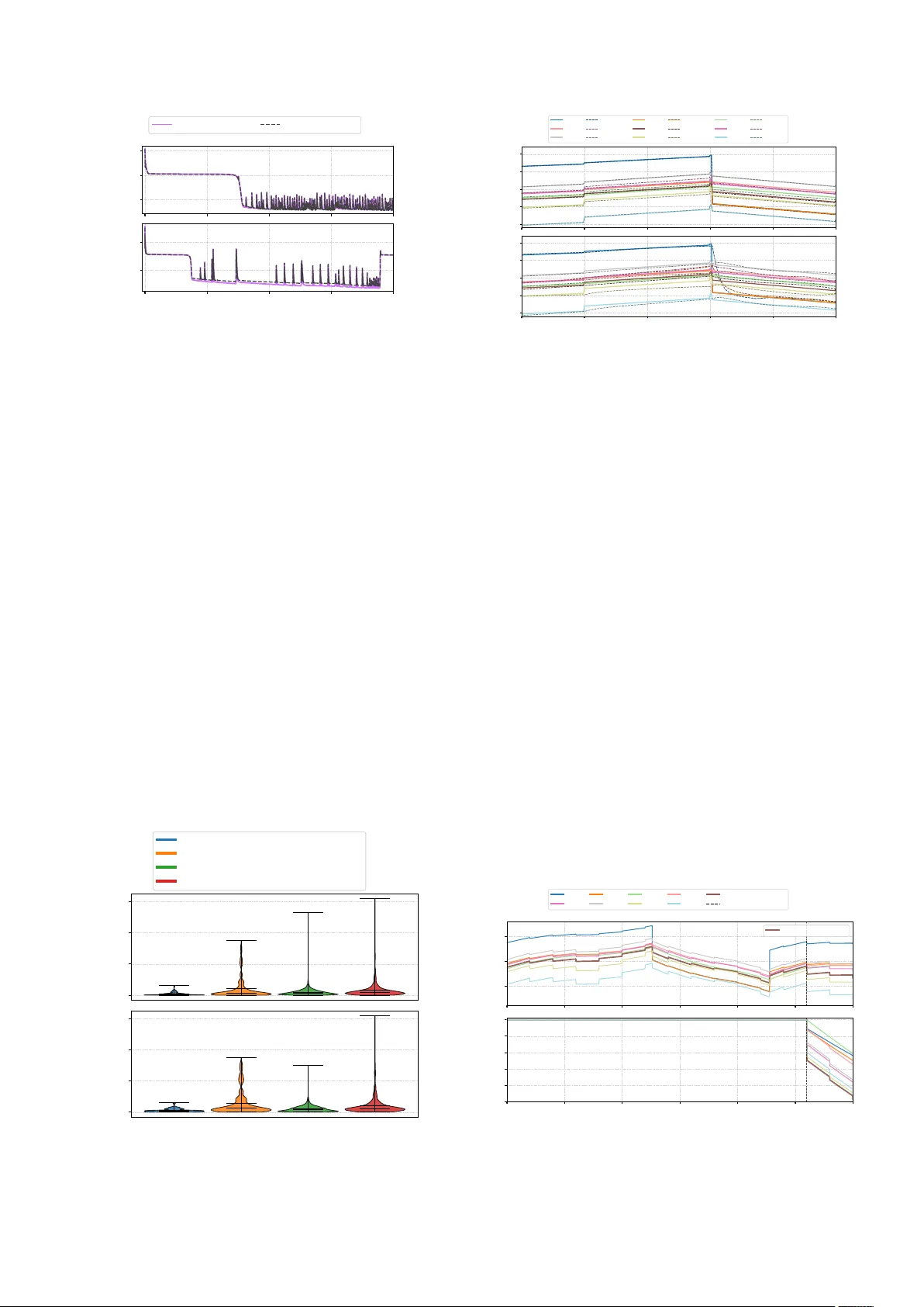
The impact of sensor placemen t on graph-neural-net w ork-based leak age detection ⋆ J.J.H.v.Gemert ∗ V. Bresc hi ∗ D.R. Y n tema ∗∗ K.J. Keesman ∗∗∗ M. Lazar ∗ ∗ Contr ol Systems Gr oup, Dept. of Ele ctric al Engine ering, Eindhoven University of T e chnolo gy, 5600MB Eindhoven, The Netherlands (e-mail: J.J.H.v.Gemert@tue.nl). ∗∗ W etsus, Centr e of Exc el lenc e for Sustainable W ater T e chnolo gy, 8900MA L e euwar den, The Netherlands. ∗∗∗ Mathematic al and Statistic al Metho ds – Biometris, W ageningen University, 6708PB W ageningen, the Netherlands Abstract: Sensor placemen t for leak age detection in water distribution net w orks is an imp ortan t and practical challenge for water utilities. Recen t w ork has shown that graph neural netw orks can estimate and predict pressures and detect leaks, but their p erformance strongly dep ends on the a v ailable sensor measurements and configurations. In this pap er, we inv estigate how sensor placemen t influences the p erformance of GNN-based leak age detection. W e propose a no vel P ageRank-Centralit y-based sensor placement method and demonstrate that it substantially impacts reconstruction, prediction, and leak age detection on the EP ANET Net1. Keywor ds: Sensor placement, W ater resource system mo deling and control, graph neural net works, leak age dete ction, P ageRank cen trality . 1. INTR ODUCTION Leak ages in w ater distribution netw orks (WDNs) can lead to considerable w ater losses, increased op erational costs, and infrastructure damage. Beyond these financial and structural impacts, leak ages ma y also p ose public-health risks due to the p oten tial ingress of contaminan ts (Xu et al., 2014). These c hallenges are becoming even more pressing as water scarcity becomes an increasing prob- lem under the effects of climate change, highlighting the need for effective leak age detection and leak age reduction strategies (Annaswam y et al., 2024; Qi et al., 2024). In this con text, effective leak age detection is a critical concern for man y w ater utilities, whic h t ypically rely on t wo estab- lished metho ds. The first is Minimum Nigh t Flo w (MNF) analysis, which assumes that nigh t-time demand is low and predictable, th us an y significan t increase in flo w during these hours can be in terpreted as a leak age (AL-W ashali et al., 2018; Lee et al., 2022). Ho wev er, such assumptions often do not hold in practice due to irregular demand patterns, which can limit the reliabilit y of MNF-based detection. The second approac h is mo del-based residual ⋆ This work w as performed in the co op eration framework of W etsus, European Centre of Excellence for Sustainable W ater T echnology (www.wetsus.nl). W etsus is co-funded by the European Union (Hori- zon Europ e, LIFE, Interreg and EDRF), the Province of F ryslân and the Dutch Gov ernment: Ministry of Economic Affairs (TTT, SBO & PPS-I/TKI W ater T echnology), Ministry of Education, Culture and Science (TTT & SBO) and Ministry of Infrastructure and W ater Management (National Gro wth F und - UPPW A TER). The authors like to thank the participants of the research theme “Smart W ater Grids” for the fruitful discussions and their financial supp ort. analysis, in whic h measured and reconstructed pressures are compared with predicted pressures obtained from hy- draulic models such as EP ANET or InfoW orks (Hu et al., 2021). A leak is indicated when the resulting residuals, i.e., the difference b et ween reconstructed and predicted pressures, exceed a predefined threshold. The reliability of this metho d dep ends strongly on mo del qualit y , which in turn relies on accurate real-time data, demand estimates, and hydraulic parameter v alues. Thus, uncertainties in an y of these key factors can significan tly influence leak age detection p erformance. These c hallenges hav e motiv ated interest in learning-based metho ds that reconstruct pressures directly from sen- sor measurements and do not dep end on accurate hy- draulic parameters. More sp ecifically , graph neural net- w orks (GNNs) ha ve gained attention, as they exploit the WDN’s graph top ology to learn how pressure propagates through the netw ork, enabling reconstruction at unob- serv ed junctions ev en with only a few sensors (Ha jgató et al., 2021). Several GNN architectures ha ve been ex- plored in this con text, including spectral metho ds such as ChebNet (Ha jgató et al., 2021) and hierarchical graph net works such as the graph U-Net in (T ruong et al., 2024). Neural net works hav e also b een applied directly to leak- age detection. Examples include the ANN-based pip eline leak age diagnosis in (Pérez-Pérez et al., 2021), whic h detects leak-induce d pressure disturbances from sensor data, and the GNN reconstructor–predictor framework in (Garðarsson et al., 2022), which iden tifies leaks by compar- ing reconstructed and one-step-ahead predicted pressures. Despite these adv ances, the effectiv eness of such GNN- based metho ds still dep ends on a fundamental factor: the underlying sensor configuration of the netw ork. In most existing works, the sensor lay out is fixed a priori or chosen randomly (Garðarsson et al., 2022), and its influence on reconstruction accuracy , prediction p erformance, or the o verall leak age-detection pro cess is not explicitly exam- ined. How ev er, this part is critical, as the informativeness of the pressure measuremen ts, and thereby the o verall p er- formance, is intrinsically tied to the sensor configuration. Sensor placement for leak age detection has b een widely studied in b oth industry and academia. In practice, util- ities often rely on simulation-based metho ds, where dif- feren t sensor configurations are ev aluated against a set of explored sim ulated leak scenarios (Santos-Ruiz et al., 2022; Romero-Ben et al., 2022). These approaches target leak age detection and reflect realistic op erating conditions. Ho wev er, their p erformance is limited to the finite set of sim ulated scenarios, and they do not pro vide formal guaran tees. T o address this, recent works hav e explored observ abilit y theory as a basis for sensor placement. In this framew ork, ensuring observ ability guaran tees that pres- sures at unmeasured junctions can b e reconstructed from the av ailable sensor data ov er a finite time. F or example, approac hes such as (Geelen et al., 2021; Bopardik ar, 2021) aim to maximize leak detectability by maximizing the “degree” of observ ability . These metho ds, how ever, require accurate h ydraulic parameters, demand patterns, and full mo del kno wledge, which can b e difficult to obtain in prac- tice. T o o vercome this challenge, recent work has prop osed structural observ ability–based sensor placement metho ds that rely solely on the WDN top ology and guaran tee observ abilit y without requiring any hydraulic information (v an Gemert et al., 2025a,b). While effective, the result- ing sensor configurations are often conserv ative and may demand more sensors than is feasible in practice given installation and cost constraints. Giv en the ab ov e challenges, this paper prop oses a no vel, scalable, top ology-based, and mo del-free sensor placemen t metho d based on PageRank Centralit y . W e examine how the resulting PageRank-Cen trality-based sensor placement fits with the ChebNet reconstructor–predictor framew ork and how it affects pressure reconstruction, one-step pre- diction, and residual-based leak age detection. Using the EP ANET Net1 b enc hmark, w e compare this approac h with an arbitrary configuration and ev aluate the influence of sensor placement on reconstruction accuracy , prediction p erformance, and leak age detection. The remainder of this pap er is structured as follows. Sec- tion 2 introduces the necessary preliminaries, including basic graph-theoretic concepts, the WDN setting, and the problem form ulation. Section 3 presents the main con- tributions, starting with the PageRank-Cen tralit y-based sensor placement, follow ed b y the ChebNet reconstruc- tor–predictor framew ork for pressure reconstruction and one-step prediction, and the asso ciated residual-based leak age detection mechanism. Section 4 ev aluates the ap- proac h on the EP ANET Net1 b enc hmark. Finally , Section 5 summarizes the findings and outlines directions for fu- ture research. Basic notation: Let R denote the field of real num b ers, and let R ≥ 0 and R > 0 denote the sets of non-negative and p ositiv e reals, resp ectively . F or a vector x ∈ R n , x i denotes its i -th elemen t, and 1 n ∈ R n denotes the v ector of all ones. F or a matrix A ∈ R n × n , A − 1 denotes its inv erse, and a ij the element on ro w i and column j . The n × n iden tity matrix is denoted by I n . 2. PRELIMINARIES AND PROBLEM ST A TEMENT In this section, we introduce the basic graph-theoretic concepts that provide the foundations for the sensor place- men t algorithm, GNNs, and WDN modeling, along with the general WDN setting and the problem formulation. 2.1 Basic gr aph notions & WDNs In this paper, w e consider only undirected and unw eighted graphs. A graph is undirected if ev ery edge is bidirectional, i.e., an edge from no de i to no de j implies an edge from j to i , and it is unw eigh ted if all edge w eights are equal to 1 . W e define a graph as G = ( V , E ) , where V = { v i } n i =1 is the set of no des, and E = { e k } m k =1 is the set of edges. The adjacency matrix A ∈ R n × n represen ts the topology of such a graph, where a ij = ( 1 , if edge e k connects v i and v j , 0 , otherwise . (1) Giv en the adjacency matrix, the out-de gr e e and in-de gr e e of a no de v i are defined as d out i = n X j =1 a ij , d in i = n X j =1 a j i . F or an undirected graph, we hav e that a ij = a j i for all no de pairs ( i, j ) . As a consequence, the in-degree and out- degree of each no de coincide, and we simply write d in i = d out i = d i = n X j =1 a ij , whose v alues form the diagonal entries of the degree matrix D = diag( d 1 , . . . , d n ) . (2) The graph Laplacian is then defined as L = D − A, (3) and captures how each no de relates to its neigh b ors and its connectivit y . Because of this structural role, the Laplacian is central to spectral GNNs and forms the foundation of the Chebyshev graph conv olutions used later in this pap er. Fig. 1. Illustration of EP ANET Net1 WDN consisting of t wo reservoirs/tanks (black icons), one pump (black circle), and junctions (blue circles) connected through pip es (blue lines). Fig. 2. Pro cessing pip eline from WDN top ology to Chebnet input. Before formulating the problem, we first describ e the WDN setting in which it is p osed. A WDN is an infrastruc- ture system that delivers pressurized drinking water from supply sources to consumers through an in terconnected pip e net work. A WDN t ypically consists of reserv oirs and tanks that pro vide hydraulic head, pumps that maintain pressure, pip es that transp ort water, and junctions where w ater is distributed tow ards consumer demands. An illus- tration of a small WDN is shown in Fig. 1. The top ology of this net work can b e represented by an adjacency matrix of the form defined in (1), which captures how these junctions, tanks, and reserv oirs are link ed through the pip e net work. 2.2 Pr oblem formulation Giv en a WDN such as the one illustrated in Fig. 1, we first establish the setting for the sensor placement problem. In practice, pressure sensors are t ypically installed only at junctions, whereas tanks, reservoirs, and pumps are often already equipped with sensors and treated as b oundary no des within the h ydraulic model. Consisten t with this, w e therefore consider only junctions as candidate lo cations for pressure sensors. The ov erall w orkflow of the sensor placemen t pip eline is shown in Fig. 2. Building on this setting and the challenges highlighted in Section 1, we in vestigate the following question: How c an we exploit gr aph top olo gy and c onne ctivity for sensor plac ements that enhanc e pr essur e r e c onstruction and pr e- diction ac cur acy, ther eby impr oving le akage dete ction in GNN-b ase d metho ds? The main problem will b e addressed in three steps: (i) a top ology-based sensor placement metho d is introduced, based on PageRank Centralit y; (ii) a ChebNet reconstruc- tor–predictor framework is used for pressure reconstruc- tion and one-step prediction from the resulting sparse measuremen ts; and (iii) residual analysis is applied to detect leak ages b y comparing reconstructed and predicted pressures. These comp onents are then connected through a consisten t graph construction that ensures the P ageRank- Cen trality-based sensor placement and the ChebNet archi- tecture op erate on the same underlying top ology . 3. MAIN RESUL TS In this section, we develop the metho dology outlined ab o ve. W e first in tro duce a topology-based sensor place- men t metho d using PageRank Cen trality , whic h selects an informativ e sparse set of sensors. W e then describ e the ChebNet architecture used for pressure reconstruction and one-step prediction (Ha jgató et al., 2021), together with the residual-based leak age detection framework from (Garðarsson et al., 2022). Finally , we demonstrate ho w the P ageRank-based sensor placemen t aligns with the Cheb- Net arc hitecture through a consistent graph construction. 3.1 PageR ank-Centr ality-b ase d Sensor Plac ement Using the graph representation introduced in Section 2, we no w define a top ology-based, model-free sensor placemen t metho d. The approach is based on P ageRank Centralit y (Brin and Page, 1998), which ev aluates ho w a simple random walk mov es through the netw ork. Junctions that the random walk reac hes least often are particularly inter- esting to measure when only a small n umber of sensors can b e installed. Their pressure v alues are the most difficult for a GNN to estimate from neighboring junctions. T o formalize this method, we express PageRank Cen trality on the WDN topology . W e b egin with the random-w alk transition matrix M = AD − 1 , (4) where A is the adjacency matrix (1) and D the degree matrix (2). The entry M j i giv es the probabilit y that a random walk er lo cated at junction i mov es to junction j in one step. The P ageRank algorithm augments this basic random walk using a uniform vector v = 1 n 1 n . (5) and a damping factor α ∈ (0 , 1) , resulting in the iteration p ( k +1) = αM p ( k ) + (1 − α ) v, (6) starting from p (0) = v . At eac h iteration, the pro duct M p ( k ) p erforms a random-w alk update, distributing the curren t scores across neighboring junctions according to M , while the term (1 − α ) v redistributes a uniform amoun t across all junctions. Rep eated application of (6) con verges to a unique vector p ∗ satisfying p ∗ = ( I − αM ) − 1 (1 − α ) v , (7) whic h quantifies ho w accessible each junction is under the mo dified random walk: frequently visited junctions obtain larger v alues, whereas rarely visited ones receiv e smaller v alues. Algorithm 1 demonstrates the resulting sensor placemen t using this PageRank Centralit y formulation. F or a desired n umber of sensors s , the algorithm constructs the degree and transition matrices (line 1), applies the PageRank iteration un til con vergence (lines 2–5), and then selects the s junctions with the smallest P ageRank v alues (line 6) for the c hosen sensor lo cations. These junctions provide an informativ e sensor lo cation, as their pressures are difficult to estimate from neighboring measuremen ts based on their P ageRank Centralit y v alue. Ha ving defined this top ology-driven sensor placement metho d, we now introduce the ChebNet architecture, whic h uses the resulting sparse pressure measurements to estimate the pressures throughout the WDN. Algorithm 1 PageRank-Cen trality-based Sensor Place- men t Require: A djacency matrix A ∈ { 0 , 1 } n × n , n umber of sensors s , α ∈ (0 , 1) , tolerance ε > 0 . Ensure: Sensor index set S . 1: d ← A 1 , D ← diag( d ) , M ← AD − 1 2: p (0) ← 1 n 1 , v ← 1 n 1 n 3: rep eat 4: p ( k +1) ← αM p ( k ) + (1 − α ) v 5: un til ∥ p ( k +1) − p ( k ) ∥ 2 ≤ ε 6: Sort p ( k +1) in ascending order and let S b e the indices of the s smallest entries return S 3.2 ChebNet A r chite ctur e for Pr essur e R e c onstruction and Pr e diction W e now introduce the ChebNet architecture, which serv es as the reconstruction–prediction mo del throughout this pap er. ChebNet is a spectral graph neural net work that applies Chebyshev p olynomial filters to a scaled Laplacian of the WDN top ology , enabling it to learn how pressures propagate across the junction graph from sparse measure- men ts. The graph conv olution used in ChebNet b egins with the normalized Laplacian based on the Laplacian defined in (3) L norm = I − D − 1 / 2 AD − 1 / 2 . constructed from the junction-only WDN adjacency ma- trix A and degree matrix D . Because the eigen v alues of L norm lie in [0 , 2] , it is rescaled ˆ L = 2 λ max L norm − I , (8) so that its eigen v alues lie within [ − 1 , 1] , the region where Cheb yshev p olynomials are n umerically stable (Ha jgató et al., 2021). With this scaled op erator in place, the Cheb yshev p olynomials used in the con volution are defined recursiv ely as T 0 ( ˆ L ) = I , T 1 ( ˆ L ) = ˆ L, T k ( ˆ L ) = 2 ˆ L T k − 1 ( ˆ L ) − T k − 2 ( ˆ L ) , k ≥ 2 . (9) A ChebNet lay er then ev aluates the truncated expansion g Θ ( ˆ L ) x = K X k =0 Θ k T k ( ˆ L ) x, (10) where K is the filter order and Θ k ∈ R F in × F out are the learnable weigh ts. This construction lets the net work com bine information across m ultiple hops in the junction graph, in a w a y that is directly gov erned b y the WDN top ology . With these con volutional la yers in place, we can train ChebNet to reconstruct no dal pressures from sparse mea- suremen ts as follows. Let x ( t ) ∈ R n denote the pressure v ector at time t , and let m ∈ { 0 , 1 } n indicate the sensor lo cations. The observed signal is x obs ( t ) = m ⊙ x ( t ) , (11) where ⊙ denotes the Hadamard pro duct. F rom these sparse inputs, the reconstructor learns the mapping ˆ x r ( t ) = f Θ ( x obs ( t ) , m ) , (12) whic h reconstructs the full pressure vector at time t . T o train this mo del, we use pressure tra jectories x T = { x (0) , x (1) , . . . , x ( T ) } ∈ R N , generated using a h ydraulic simulator such as EP ANET. Applying the mask (11) yields the inputs x obs ( t ) , and the parameters of the reconstructor are optimized by minimizing L rec (Θ) = 1 T T X t =1   f Θ ( x obs ( t ) , m ) − x ( t )   2 2 . (13) This mo del acts as a static estimator, it reconstructs the pressure at time t using only the measu remen ts a v ailable at that same instant. T o capture temp oral b ehaviour instead of static, w e extend this architecture to a pr e dictor that estimates x ( t + 1) from a window of past measurements. T o formalize this, for a windo w length w ∈ N w e define x w ( t ) =  x ( t − w + 1) , x ( t − w + 2) , . . . , x ( t )  , x obs w ( t ) = m ⊙ x w ( t ) . The predictor learns the mapping ˆ x p ( t + 1) = f ϕ  x obs w ( t ) , m  . (14) F or training the predictor, let T tr denote the set of time indices used for one-step prediction, and let N tr b e its cardinalit y . The predictor parameters are obtained b y minimizing L pred ( ϕ ) = 1 N tr X t ∈ T tr   f ϕ  x obs w ( t ) , m  − x ( t + 1)   2 2 . (15) Ha ving both mo dels in place, leak age detection is based on the residuals of the reconstruction and the prediction. W e define the no dal residual r n ( t ) = ˆ x r ( t ) − ˆ x p ( t ) , whic h remains small under leak-free conditions. Because leaks o ccur along pip es rather than at junctions, these no dal residuals are pro jected onto edges r e ( t ) =   r n i ( t ) − r n j ( t )   . Finally , to reduce the effect of noise and short-term fluc- tuations, we apply a rolling window of length m r to the absolute edge residuals, yielding the smo othed residuals ¯ r e ( t ) = 1 m r t X τ = t − m r +1 r e ( τ ) . T o detect abnormal b eha vior, i.e., a leak, we construct a threshold based on the leak-free training data. Let µ e and σ e denote the mean and standard deviation of ¯ r e ( t ) o ver the health y v alidation set. A leak alarm is raised on edge e when ¯ r e ( t ) > µ e + α a σ e , where α a > 0 is a tuning parameter that balances sensi- tivit y and false-alarm rate. 3.3 Consistent Gr aph Construction for PageR ank and ChebNet T o connect the PageRank-Cen trality-based sensor place- men t with the ChebNet reconstructor–predictor frame- w ork, b oth must op erate on the same underlying graph. F ollo wing the assumptions in Section 2 and the definition of ˆ L in (8), pressure sensors are placed only at junctions, while tanks, reserv oirs, and pumps act as b oundary no des. Extracting the junction–junction connectivity from the Fig. 3. ChebNet architecture for pressure reconstruction and prediction in water distribution netw orks (WDNs). h ydraulic mo del results in a symmetric adjacency matrix A ∈ { 0 , 1 } n × n , where n is the n umber of junctions. This same matrix defines the transition matrix M = AD − 1 used in the P ageRank iteration (6), and through the normalized and scaled Laplacian, it also determines the ChebNet graph con volution. F or example, the junction- only adjacency matrix of the EP ANET Net1 (Fig. 1) is A =             0 1 0 0 0 0 0 0 0 1 0 1 0 1 0 0 0 0 0 1 0 1 0 1 0 0 0 0 0 1 0 0 0 1 0 0 0 1 0 0 0 1 0 1 0 0 0 1 0 1 0 1 0 1 0 0 0 1 0 1 0 0 0 0 0 0 0 1 0 0 0 1 0 0 0 0 0 1 0 1 0             . (16) Using this unified adjacency matrix ensures full consis- tency: the P ageRank-Centralit y-based sensor placement selects junctions based on the same connectivity that de - termines how ChebNet propagates information through its sp ectral filters. P ageRank uses A to drive the random-walk dynamics, and ChebNet builds its Laplacian filters directly from A . As a result, reconstruction, prediction, and leak age detection all op erate on a graph that is structurally aligned with the sensor placemen t strategy , ensuring that sensor placemen t and ChebNet filtering are fully aligned in terms of the underlying graph structure. 4. SIMULA TION RESUL TS In this section, we compare the PageRank-Cen trality- based sensor placemen t with an arbitrary placement of equal size on the EP ANET Net1 net work. F or clarity , the analysis is structured into three parts: (i) the sensor placemen t and training setup, (ii) v alidation and testing of the reconstructor and predictor, and (iii) leak age detection under a simulated fault. 4.1 Sensor plac ement and tr aining T o obtain the PageRank-cen tralit y-based sensor place- men t in Algorithm 1, we compute the PageRank scores of the junction-only adjacency matrix in (16), using a damp- ing factor α p = 0 . 85 . T able 1 sho ws the resulting ranking, ordered from low est to highest PageRank v alue. Selecting the three low est-ranked junctions yields the sensor set { 10 , 23 , 32 } . F or comparison, w e include an arbitrary placemen t of the same size, chosen to hav e a similar spatial distribution without ov erlapping sensor lo cations, namely { 13 , 22 , 31 } . Note that the no de iden tifiers in T able 1 corresp ond to the EP ANET junction lab els (as in Fig. 1), not to the row or column indices of the adjacency matrix. T able 1. PageRank v alues for Net1 in Fig. 1, computed using A in (16) with α p = 0 . 85 . Node 10 23 32 13 31 21 12 11 22 p 0.056 0.092 0.092 0.093 0.093 0.132 0.132 0.139 0.1699 F or each sensor configuration, we train a ChebNet recon- structor and predictor, resulting in four GNNs in total. Using EP ANET, w e generate a 108 -hour dataset with a 1- min ute sampling interv al ( 6480 samples), of whic h the first 60 hours are used for training, hours 60 – 84 for v alidation, and the final 24 hours for testing. The predictor uses a temp oral windo w of w = 120 minutes. All GNNs use a four-la yer ChebNet architecture with Chebyshev orders K = [48 , 24 , 4 , 1] and channel widths F = [24 , 12 , 6] , rep- resen ting a scaled-down but structurally consisten t version of the design used for the L-T own net work in (Garðarsson et al., 2022). T able 2. T raining and v alidation mean squared errors (MSE) for the four GNNs on Net1. GNN T raining MSE V alidation MSE Reconstructor (PageRank) 0.1452 0.1358 Reconstructor (Arbitrary) 3.910 4.407 Predictor (PageRank) 0.4092 0.6831 Predictor (Arbitrary) 2.848 3.582 T able 2 summarizes the final training and v alidation er- rors for all four GNNs. The reconstructor and predic- tor trained with the P ageRank-Centralit y-based sensor placemen t achiev e consistently lo wer v alidation errors than those trained with arbitrary placement, indicating that the P ageRank-Centralit y-based sensor configuration pro vides more informativ e measurements. Additionally , for b oth sensor configurations, the predictor results in higher errors than the reconstructor. This b ehavior is also visible in the training curves in Fig. 4. The reconstructor con verges quic kly and stabilizes at a low loss with only minor fluctu- ations, whereas the predictor sho ws larger oscillations and a higher ov erall loss. 10 0 10 2 10 4  rec (a) 0 2500 5000 7500 10000 Epoch 10 1 10 3  pred (b) Training loss V alidation loss Fig. 4. T raining and v alidation loss on a logarithmic scale for the reconstructor (a) and predictor (b), using P ageRank-Centralit y-based sensor placement. 4.2 T esting of the r e c onstructor and pr e dictor T o compare the reconstruction and prediction p erfor- mance, we examine the residual distributions of all four GNNs b y sho wing violin plots for all junctions and for the non-sensed junctions in Figure 5. F rom Figure 5, w e observ e the same b ehaviour as in T able 2, i.e., the P ageRank-Centralit y-based sensor placemen t yields nar- ro wer and more concentrated residuals, indicating higher reconstruction and prediction accuracy , whereas the arbi- trary placement results in broader distributions. A ddition- ally , we again see that the predictor consistently pro duces larger residuals than the reconstructor, since it must learn one-step-ahead dynamics instead of a static mapping. This mak es the predictor more sensitive to abrupt c hanges in the pressure tra jectory , particularly at the demand-driven discon tinuities, whic h are visible in Fig. 6. 4.3 L e akage simulation setup and dete ction Ha ving established the four GNNs, w e now compare both sensor configurations in a leak age scenario. T o this end, Net1 is simulated for 30 hours with a 1-min ute resolution, and a single leak is introduced at hour 26 by activ ating the 0 5 10 15 (a) 0 5 10 15 (b) Absolute error in pressure head [m] Reconstructor – P ageR ank placement Reconstructor – Arbitrary placement Predictor – P ageR ank placement Predictor – Arbitrary placement Fig. 5. Residual distributions for the four GNNs on Net1, sho wn as violin plots ov er all junctions in (a) and ov er non-sensed junctions in (b). 115 120 125 130 135 Pressure head [m] (a) 11 12 13 14 15 16 Time [h] 115 120 125 130 135 Pressure head [m] (b) 10 13 23 Est 10 Est 13 Est 23 11 21 31 Est 11 Est 21 Est 31 12 22 32 Est 12 Est 22 Est 32 Fig. 6. T rue vs. reconstructed pressures in (a) and true vs. one-step-ahead predictions in (b). emitter co efficient at junc tion 21 (Fig. 1). This junction is not sensed in both configurations but lies adjacen t to a junction equipp ed with either a P ageRank-Centralit y- based sensor or an arbitrary sensor. The leak magnitude is chosen suc h that the resulting head drop exceeds t ypical demand-driv en discontin uities (ab out 1.5 m), ensu ring that the even t is distinguishable from normal v ariations. Figure 7 shows the resulting pressure tra jectories and the corresp onding pressure deviations, with the leaky junction highligh ted. F or b oth sensor configurations, we apply the same residual-based detection criterion introduced in Sec- tion 3.2 using m r = 150 and α a = 6 . The leak age alarm timelines are shown in Fig. 8. The red dashed line marks the leak start time at 26 h and the colored interv als indicate p erio ds during whic h the residual-based detection triggers an alarm. Before the leak starts, b oth configurations trigger false alarms due to the demand-driven pressure discontin u- ities that momentarily increase the prediction error. The P ageRank-Centralit y-based placement is noticeably less sensitiv e to these discon tinuities, its alarms are shorter, and the detector returns more quickly to the no-alarm state. In con trast, the arbitrary placemen t reacts more strongly to the same discon tin uities, resulting in longer false-alarm p erio ds. Once the leak b egins, the PageRank- Cen trality-based placement raises an alarm immediately 110 120 130 Pressure head [m] (a) Leaky junction (21) 0 5 10 15 20 25 30 Time [h] −5 −4 −3 −2 −1 0 Pressure residual [m] (b) 10 22 11 23 12 31 13 32 21 Leakage start time Fig. 7. Leak age simulation in Net1: (a) pressure tra jecto- ries with the leaky junction highlighted, (b) pressure differences relative to leak-free conditions. No alarm Alarm 0 5 10 15 20 25 30 Time [h] No alarm Alarm Alarm (arbitrary placement) Alarm (PageRank placement) Leak start Fig. 8. Comparison leak alarms for PageRank-Cen tralit y- based and arbitrary sensor placements on Net1. and main tains it for a longer interv al than any of its false alarms. The arbitrary placement resp onds only after roughly 30 min utes and produces a shorter alarm, even though its false-alarm p erio ds are longer. This b eha viour reflects the impro ved reconstruction–prediction accuracy with the PageRank-Cen trality-based sensor placement. 5. CONCLUSION AND FUTURE WORK This pap er in vestigated ho w P ageRank-Centralit y-based sensor placemen t influences the p erformance of a Cheb- Net architecture for pressure reconstruction, one-step- ahead prediction, and leak age detection in w ater distribu- tion net works. Using the EP ANET Net1 b enchmark, we demonstrated that selecting sensors based on PageRank Cen trality yields more informative measurement lo cations, resulting in lo wer reconstruction and prediction errors and significantly reduced false-alarm time compared to an arbitrary sensor placemen t. These improv ements were observ ed b oth in normal operation and under a leak age scenario. Additionally , the predictor consistently show ed larger residuals than the reconstructor, whic h could b e explained b y the abrupt pressure discontin uities driven by the demand pattern. F or future work, sev eral c hallenges could b e explored. First, incorporating smo other and more realistic demand patterns may help reduce the discon tinuit y-driven pre- diction errors observed in the current setup. In practice, suc h sharp pressure steps rarely o ccur except during pip e bursts, normal demand v ariations pro duce muc h gen tler c hanges. Second, further improv ements to the architecture could fo cus on handling these sharp transients more effec- tiv ely . Third, a robust metho d for distinguishing demand- driv en pressure drops from leak-induced deviations re- mains an imp ortant op en question. Finally , applying the P ageRank-Centralit y-based sensor placement to larger and more complex net works would allo w for the assessment of scalabilit y and generalization. REFERENCES AL-W ashali, T., Sharma, S., AL-Nozaily , F., Haidera, M., and Kennedy , M. (2018). Mo delling the leak age rate and reduction using minimum nigh t flow analysis in an in termittent supply system. W ater , 11(1), 48. Annasw amy , A.M., Johansson, K.H., and Pappas, G. (2024). Con trol for so cietal-scale challenges: Road map 2030. IEEE Contr ol Systems Magazine , 44(3), 30–32. Bopardik ar, S.D. (2021). A randomized approac h to sensor placemen t with observ abilit y assurance. Automatic a , 123, 109340. Brin, S. and Page, L. (1998). The anatomy of a large-scale h yp ertextual web search engine. Computer networks and ISDN systems , 30(1-7), 107–117. Garðarsson, G.Ö., Bo em, F., and T oni, L. (2022). Graph- based learning for leak detection and lo calisation in wa- ter distribution netw orks. IF A C-Pap ersOnLine , 55(6), 661–666. Geelen, C.V., Y ntema, D.R., Molenaar, J., and Keesman, K.J. (2021). Optimal sensor placement in h ydraulic con- duit net works: A state-space approach. W ater , 13(21), 3105. Ha jgató, G., Gyires-Tóth, B., and P aál, G. (2021). Re- constructing no dal pressures in water distribution sys- tems with graph neural net works. arXiv pr eprint arXiv:2104.13619 . Hu, Z., Chen, B., Chen, W., T an, D., and Shen, D. (2021). Review of mo del-based and data-driven approaches for leak detection and location in w ater distribution sys- tems. W ater Supply , 21(7), 3282–3306. Lee, S.S., Lee, H.H., and Lee, Y.J. (2022). Prediction of minimum night flow for enhancing leak age detection capabilities in water distribution netw orks. Applie d Scienc es , 12(13), 6467. Pérez-Pérez, E.d.J., Lóp ez-Estrada, F.R., V alencia- P alomo, G., T orres, L., Puig, V., and Mina-Antonio, J.D. (2021). Leak diagnosis in pipelines using a com- bined artificial neural netw ork approac h. Contr ol Engi- ne ering Pr actic e , 107, 104677. Qi, R., Cao, M., and Y ntema, D.R. (2024). Recen t devel- opmen ts of subsurface small-leak detection techniques in w ater distribution netw orks: A review. IEEE R ob otics & Automation Magazine , 31(1), 108–118. Romero-Ben, L., Cembrano, G., Puig, V., and Blesa, J. (2022). Mo del-free sensor placemen t for water distribu- tion net works u sing genetic algorithms and clustering. IF A C-Pap ersOnLine , 55(33), 54–59. San tos-Ruiz, I., López-Estrada, F.R., Puig, V., V alencia- P alomo, G., and Hernández, H.R. (2022). Pressure sen- sor placement for leak lo calization in water distribution net works using information theory . Sensors , 22(2), 443. T ruong, H., T ello, A., Lazovik, A., and Degeler, V. (2024). Graph neural netw orks for pressure estimation in water distribution systems. W ater R esour c es R ese ar ch , 60(7), e2023WR036741. v an Gemert, J., Breschi, V., Y ntema, D.R., Keesman, K.J., and Lazar, M. (2025a). Exploiting structural observ abilit y and graph colorabilit y for optimal sensor placemen t in water distribution netw orks. In 2025 Eur op e an Contr ol Confer enc e (ECC) , 546–551. v an Gemert, J., Bresc hi, V., Y ntema, D.R., Keesman, K.J., and Lazar, M. (2025b). Scalable sensor placement for cyclic netw orks with observ ability guarantees: Appli- cation to water distribution net w orks. arXiv pr eprint arXiv:2412.09965 . (accepted for the CDC 2025). Xu, Q., Liu, R., Chen, Q., and Li, R. (2014). Review on w ater leak age con trol in distribution netw orks and the asso ciated environmen tal b enefits. Journal of Envir on- mental Scienc es , 26(5), 955–961.