Blind Quality Enhancement for G-PCC Compressed Dynamic Point Clouds

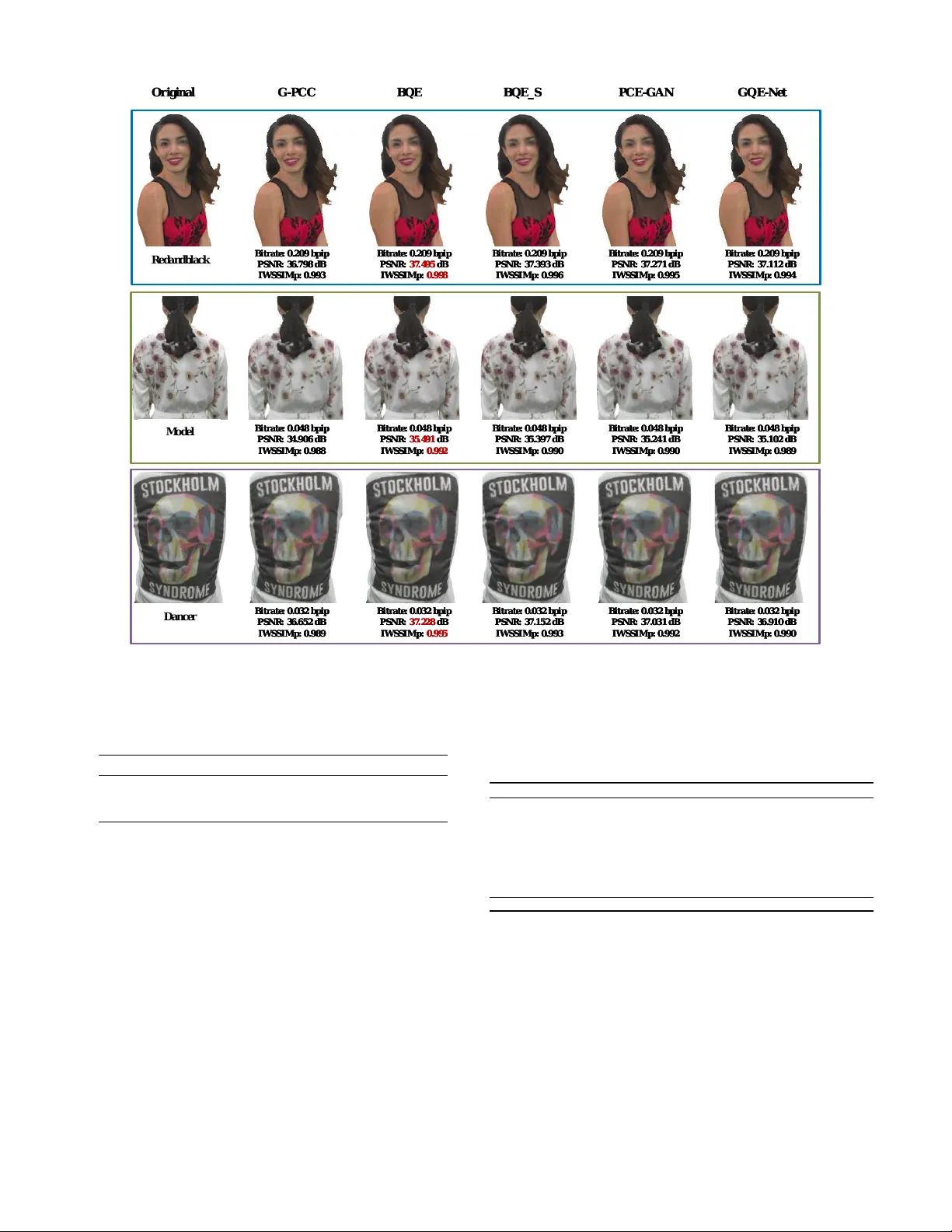
JOURNAL OF L A T E X CLASS FILES, VOL. 14, NO. 8, A UGUST 2021 1 Blind Quality Enhancement for G-PCC Compressed Dynamic Point Clouds T ian Guo, Hui Y uan, Senior Member , IEEE, Chang Sun, W ei Zhang, Senior Member , IEEE , Raouf Hamzaoui, Senior Member , IEEE , and Sam Kwong, F ellow , IEEE Abstract —Point cloud compression often introduces noticeable reconstruction artifacts, which makes quality enhancement nec- essary . Existing approaches typically assume prior knowledge of the distortion level and train multiple models with identical architectur es, each designed f or a specific distortion setting. This significantly limits their practical applicability in scenarios where the distortion level is unknown and computational resources are limited. T o overcome these limitations, we propose the first blind quality enhancement (BQE) model f or compressed dynamic point clouds. BQE enhances compressed point clouds under unknown distortion lev els by exploiting temporal dependencies and jointly modeling feature similarity and differences across multiple dis- tortion lev els. It consists of a joint progr essive feature extraction branch and an adaptive featur e fusion branch. In the joint progr essive feature extraction branch, consecutive reconstructed frames are first fed into a recoloring-based motion compensation module to generate temporally aligned virtual reference frames. These frames are then fused by a temporal correlation-guided cross-attention module and processed by a pr ogressiv e featur e extraction module to obtain hierarchical features at different distortion levels. In the adaptive feature fusion branch, the current reconstructed frame is input to a quality estimation module to predict a weighting distribution that guides the adaptive weighted fusion of these hierar chical features. When applied to the latest geometry-based point cloud compression (G- PCC) refer ence software, i.e., test model category13 version 28, BQE achieved average PSNR improv ements of 0.535 dB, 0.403 dB, and 0.453 dB, with BD-rates of -17.4%, -20.5%, and -20.1% for the Luma, Cb, and Cr components, respectively . Index T erms —Point cloud compr ession, attrib ute enhancement, blind quality enhancement, G-PCC, point cloud. I . I N T R O DU C T I O N P OINT clouds represent objects or scenes as sets of 3D points, each with geometric coordinates and associated attributes [1]–[4]. Owing to their ability to capture fine-grained spatial details, point clouds hav e been widely applied in fields such as autonomous driving, virtual reality , online education, and cultural heritage preservation [5]–[10]. Ho wev er, their massiv e data volume poses a significant challenge for efficient This work was supported in part by the National Natural Science Foundation of China under Grants 62571303, the High-end Foreign Experts Recruitment Plan of Chinese Ministry of Human Resources and Social Security under Grant H20251083. (Corresponding author: Hui Y uan) T ian Guo, Hui Y uan, Chang Sun, and W ei Zhang are with the School of Control Science and Engineering, Shandong Univ ersity , Ji’nan, 250061, China, and also with the Key Laboratory of Ma- chine Intelligence and System Control, Ministry of Education, Ji’nan, 250061, China (e-mail: guotiansdu@mail.sdu.edu.cn; huiyuan@sdu.edu.cn; 202220795@mail.sdu.edu.cn; davidzhang@sdu.edu.cn). Raouf Hamzaoui is with the School of Engineering, Infrastructure and Sustainability , De Montfort University , LE1 9BH Leicester , UK. (e-mail: rhamzaoui@dmu.ac.uk). Sam Kwong is with the Department of Computing and Decision Science, Lingnan University , Hong Kong (e-mail: samkwong@ln.edu.hk). storage and transmission. T o address this challenge, point cloud compression has been e xtensiv ely studied [11], [12]. In 2017, the Moving Picture Experts Group (MPEG) under ISO/IEC issued a call for proposals on point clouds compres- sion [13], which led to the dev elopment of the geometry-based point cloud compression (G-PCC) standard [14]. Despite these advances, lossy compression inevitably introduces irrev ersible compression artifacts, which significantly degrade the quality of reconstructed point clouds. In recent years, man y quality enhancement methods for compressed point clouds hav e been proposed. These methods are generally categorized into traditional approaches and deep learning–based approaches. Traditional methods are not data- driv en b ut rely on linear model–based filtering techniques, such as Kalman and W iener filters, whose parameters are deriv ed from assumed spatial or temporal correlations and noise statistics. Although these approaches can achie ve cer - tain improv ements, their reliance on prior models and as- sumptions limits their ability to handle div erse and complex noise patterns. For deep learning–based approaches, graph con volution [15]–[18] and sparse con volution [19]–[22] are usually adopted for efficient feature extraction. By modelling local geometric relationships on the adjacency graph or sparse vox els of the input point cloud, these methods achieve higher reconstruction quality by recovering fine structural and texture details. Although existing deep learning-based approaches hav e demonstrated excellent performance, they are non-blind qual- ity enhancement approaches. The y typically require training multiple models with the same architecture for different dis- tortion levels, which are usually controlled by the quantiza- tion parameters (QPs) of the codec. These non-blind qual- ity enhancement methods suffer from two major limitations. First, in transcoding and transmission, the exact distortion lev el is often incomplete or unkno wn, making it difficult to select an appropriate trained model. Second, handling different distortion levels with separate, structurally identical models increases deployment complexity and resource requirements, which poses challenges for real-world applications. T o address the above challenges, we propose the first blind quality enhancement (BQE) model for compressed point cloud attributes. The proposed BQE model enhances compressed point clouds under unknown distortion levels by exploiting temporal dependencies and jointly modeling feature similarity and discrepancy across different distortion le vels. It consists of two branches: a joint progressive feature extraction branch and an adaptive feature fusion branch. Specifically , consecuti ve reconstructed frames are first fed into a recoloring-based JOURNAL OF L A T E X CLASS FILES, VOL. 14, NO. 8, A UGUST 2021 2 motion compensation (RMC) module to generate temporally aligned virtual reference frames. Subsequently , a temporal correlation-guided cross-attention (TCCA) module is proposed to fuse multi-frame information and efficiently exploit tempo- ral correlations. The fused features are then processed by a progressiv e feature extraction module to obtain hierarchical representations corresponding to different distortion lev els. The adapti ve feature fusion branch takes the current recon- structed frame as input and predicts a quality v ector (i.e., a weighting distribution) across dif ferent distortion levels via a quality estimation (QE) module, which guides the fusion of the progressi vely extracted hierarchical features. In summary , the contributions of this paper are as follows. • W e propose a blind quality enhancement model for point cloud attributes that achiev es effecti ve restoration under unknown distortion levels. T o the best of our knowledge, this is the first attempt at blind quality enhancement for compressed point clouds. • W e propose a joint progressiv e feature extraction branch and an adaptiv e feature fusion branch in the BQE model. The joint progressiv e feature extraction branch captures representations across different distortion lev els, while the adaptive feature fusion branch predicts a weighting distribution to guide adapti ve feature fusion. This design enables effectiv e utilization of multi-level distortion char- acteristics and improves reconstruction quality . • W e propose a temporal correlation-guided cross-attention module that constructs a temporal interaction mecha- nism centered on the current frame to adaptively capture inter-frame correlations and dynamically assign attention weights, ef ficiently exploiting temporal information for enhancement. • W e design a neighborhood-aware attention (NA) module that uses local positional encoding to strengthen geome- try priors, enabling more efficient feature extraction for progressiv e feature extraction and weighting distribution prediction. The remainder of this paper is organized as follows. Section II revie ws related work. Section III describes the proposed method. Section IV presents experimental results and analysis. Finally , Section V concludes the paper . I I . R E L A T E D W O R K In this section, we first revie w relev ant work on non- blind point cloud quality enhancement. Then, because blind quality enhancement for point clouds has not been previously explored, we summarize representativ e blind quality enhance- ment methods for images and videos. A. Non-blind point cloud quality enhancement Non-blind point cloud quality enhancement methods can be roughly divided into two classes: traditional methods and deep learning-based methods. Early studies introduced the Kalman filter into G-PCC to enhance attribute reconstruction. Howe ver , because its effec- tiv eness relies on the stationarity assumption, the improve- ments were mainly observed in chrominance components [23]. T o further mitigate distortion accumulation during the cod- ing process, W iener filter-based methods were subsequently proposed [24], [25]. Although these approaches offer some advantages, their performance remains constrained by the undelying assumption of linear distortion. Deep learning-based methods can be broadly categorized into two categories: graph conv olution-based methods and sparse con volution-based methods. Graph con volution-based methods use geometry priors to guide attribute enhancement. Sheng et al. [26] proposed a multi-scale graph attention network to remove attrib ute artifacts caused by the G-PCC encoder . They constructed a graph based on geometry co- ordinates and used Chebyshev graph con volution to extract attribute feature representations. Xing et al. [27] introduced a graph-based quality enhancement network that uses geometry information as an auxiliary input and graph conv olution blocks to extract local features efficiently . In [28], we proposed PCE-GAN, which models point cloud attribute quality en- hancement as an optimal transport problem and explicitly integrates perceptual quality into the enhancement frame work. By using sparse 3D con volution, Liu et al. [29] proposed a dynamic point cloud enhancement method that uses inter - frame motion prediction with relativ e positional encoding and motion consistency to align the current frame with its refer- ence. Zhang et al. [30] proposed G-PCC++, which enhances the quality of both geometry and attributes. The method densifies the decoded geometry via linear interpolation to form a continuous surface, applies Gaussian distance-weighted mapping for recoloring, and further refines the results with an attribute enhancement model. Later, they [31] proposed a fully data-driv en method and a rule-unrolling-based optimization to restore G-PCC compressed point cloud attributes. Moreov er, they [32] designed a learning-based adapti ve in-loop filter for efficient quality enhancement. Howe ver , all the existing methods require prior knowl- edge of distortion lev els and separate training of multiple architecture-identical models for different distortion lev els, which results in high computational cost and limited appli- cability in real-world scenarios. Therefore, developing blind point cloud quality enhancement methods has become an urgent necessity . B. Blind image/video quality enhancement Although the data structure of images, videos, and point clouds are dif ferent, blind quality enhancement methods for compressed images and videos can still inspire the design of blind quality enhancement for compressed point cloud attributes. T o remove compression artifacts, Kim et al. [33] proposed a pseudo-blind con volutional neural network (PBCNN) that estimates the compression quality factor and uses sev eral as- sociated non-blind models to remove compression artifacts for both video and image coding standards [34], [35]. T o reduce computational costs, Xing et al. [36] proposed a resource- efficient blind quality enhancement (RBQE) method for com- pressed images. Lev eraging dynamic deep neural netw orks and no-reference quality assessment methods, RBQE enables JOURNAL OF L A T E X CLASS FILES, VOL. 14, NO. 8, A UGUST 2021 3 Fig. 1. BQE architecture. The proposed BQE model consists of two branches: a joint progressive feature extraction branch and an adaptive feature fusion branch. Given a reconstructed point cloud sequence ( ˆ P t − R , . . . , ˆ P t , . . . , ˆ P t + R ) , where ˆ P t is the target frame and the remaining frames are reference frames, the goal of blind attribute quality enhancement is to restore ˆ P t to an enhanced version e P t without knowing the distortion lev el of ˆ P t . Note that the target frame is unchanged by RMC, i.e., ˆ P ′ t = ˆ P t . blind and progressi ve enhancement with an early-exit strategy , making it highly resource-friendly . Jiang et al. [37] proposed a flexible blind CNN for JPEG artifact removal that decouples and predicts an adjustable quality factor from the input image and injects it via a quality-factor attention block to control the trade-off between artifact removal and detail preservation. Xing et al. [38] proposed a blind image compression artifact reduction recurrent network that adapts to unkno wn quality factors and dif ferent degradation lev els with scalable recurrent con volution and efficient conv olution groups. Recently , Li et al. [40], [41] proposed a prompt-learning-based compressed image restoration network, which uses prompt learning to im- plicitly encode compression information and provide dynamic content-aware and distortion-aware guidance for restoration. Finally , Ding et al. [39] proposed a blind quality enhance- ment method for compressed video that exploits fluctuating temporal information and feature correlations across multiple QPs. I I I . P R O P O SE D M E T H O D Giv en a point cloud sequence P , the t -th frame is denoted by P t = [ P G t , P A t ] , where P G t represents the geometry and P A t represents the associated attributes. Let ˆ P t = [ ˆ P G t , ˆ P A t ] be the reconstructed frame after compression. For a temporal window of radius R ∈ N , we consider the ordered windo w ( ˆ P t − R , . . . , ˆ P t , . . . , ˆ P t + R ) , which has length 2 R + 1 . W e assume lossless geometry compression, i.e., ˆ P G t = P G t , so any distortion introduced by compression is restricted to the attributes ˆ P A t . The goal of attrib ute quality enhancement is to refine the reconstructed point cloud sequence within the temporal window to obtain higher-quality attributes, using the corresponding original sequence as ground truth during train- ing (the original point clouds are not av ailable at inference). In particular , frame ˆ P t is treated as the targ et frame, while the remaining frames in the window serve as refer ence frames. The enhanced target frame is defined as ˜ P t = [ P G t , ˜ P A t ] , which preserves the geometry and refines only the attributes. W e compute ˜ P t = Ψ BQE ( ˆ P t − R , . . . , ˆ P t , . . . , ˆ P t + R ; θ ) , (1) where Ψ BQE ( · ) denotes the proposed BQE model with learn- able parameters θ . In our experiments, we set R = 2 . The proposed BQE model consists of a joint pro- gressiv e feature extraction branch and an adaptiv e fea- ture fusion branch (Fig. 1). Gi ven the ordered input win- dow ( ˆ P t − R , . . . , ˆ P t , . . . , ˆ P t + R ) , the joint branch processes the entire window , whereas the fusion branch processes the center frame ˆ P t . In the joint branch (Section III- A), the frames ( ˆ P t − R , . . . , ˆ P t + R ) are first passed through the RMC module to generate virtual reference frames ( ˆ P ′ t − R , . . . , ˆ P ′ t , . . . , ˆ P ′ t + R ) , which align the reference frames to the target frame ˆ P t . The aligned frames are then fed into the TCCA module, which models temporal correlations via multi-frame feature interaction and outputs a fused feature F o . Next, F o is forwarded to the progressive feature extrac- tion module, which extracts hierarchical features, enabling resource-efficient utilization of feature similarity across mul- tiple distortion le vels. In the adaptiv e feature fusion branch (Section III-B), the current reconstructed frame ˆ P t is first processed by the QE module to estimate a quality vector that JOURNAL OF L A T E X CLASS FILES, VOL. 14, NO. 8, A UGUST 2021 4 Fig. 2. Structure of the TCCA module. The ordered sequence ( ˆ P ′ t − R , . . . , ˆ P ′ t , . . . , ˆ P ′ t + R ) denotes the virtual frames produced by the RMC module. For notational consistency , we use a prime to indicate frames after RMC. In particular, the target frame is unchanged by RMC, i.e., ˆ P ′ t = ˆ P t . represents weighting distributions for features. The estimated quality vector is then fed into the adaptiv e fusion module to combine the progressiv ely extracted hierarchical features. A. Joint Pr ogr essive F eature Extraction Branch T o ef ficiently e xploit temporal correlations in compressed dynamic point clouds, consecutive reconstructed frames are processed jointly . The RMC module first maps the attribute in- formation of reference frames onto the geometry of the current frame to achie ve precise spatial alignment. Next, the TCCA module adaptiv ely aggregates temporal information from the reference frames by enabling information exchange between the current-frame and reference-frame features, improving the fused representation.Next, the TCCA module adaptiv ely aggregates temporal information from the reference frames by enabling information exchange between the current-frame and reference-frame features, improving the fused representation. Finally , the fused feature F o is refined by the progressiv e feature e xtraction module which learns hierarchical features across dif ferent distortion levels to achiev e ef fectiv e quality enhancement. 1) Recoloring-based Motion Compensation Module T o address the geometry and color misalignment caused by inter-frame motion in dynamic point clouds, we use the RMC module. Instead of explicitly estimating motion vectors, RMC remaps the attribute information of the reference frames to the geometry coordinates of the current frame, achieving spatial alignment and reducing motion-induced artif acts. These virtual reference frames facilitate more accurate temporal feature fusion in subsequent modules. 2) T emporal Correlation-guided Cross-Attention Module T o model temporal correlations, we propose a TCCA mod- ule that adaptively fuses information across multi-frame point clouds (Fig. 2). Specifically , the attribute of the current frame ˆ P t is first processed by a projection layer Pro j q to construct the query embedding. Meanwhile, the consecutiv e frames { ˆ P ′ t − R , . . . , ˆ P ′ t , . . . , ˆ P ′ t + R } are fed into separate projection layer Pro j k and Pro j v to generate the key and value embed- dings: F q = Pro j q ( ˆ P ′ A t ) , F k = Pro j k (Concat( ˆ P ′ A i )) , F v = Pro j v (Concat( ˆ P ′ A i )) . (2) where i ∈ { t − R, . . . , t + R } . Note that ˆ P ′ t = ˆ P t , since the target frame at time t remains unchanged after the RMC module, and the prime symbol is introduced only for notational consistency . Pro j q , Pro j k , and Pro j v refer to the projection lay- ers that comprise cascaded linear layers and LeakyReLU functions, which can be mathematically represented as Linear  LReLU  Linear  LReLU  Linear( · )  . Then, the similarity between F q and F k is computed using scaled dot-product attention, yielding the attention weights s [42]: s = Softmax( F q · F ⊤ k √ d k ) , (3) where d k denotes the embedding dimension of the keys (and queries). Next, the attention output is obtained by weighting the v alue embeddings, s F v , and projecting the result through a linear layer Pro j o to produce F t . Moreov er, we introduce a skip connection from ˆ P A t to preserve current-frame informa- tion. Finally , the resulting features are concatenated with the geometry of the current frame: F o = Concat( F t + ˆ P A t , P G t ) . (4) The fused feature F o is then forwarded to the progressive feature extraction module. 3) Progressive F eature Extraction Module The design of the progressive e xtraction module is primarily motiv ated by two key considerations. 1  Featur e similarity across multiple distortion levels: Compressed point clouds encoded by different QPs share similar feature representations in the quality enhancement task. Therefore, the feature e xtraction structures corresponding to various distortion lev els can be partially shared within a unified framew ork to improve efficienc y and consistency . 2  Context modeling requirements for high-distortion point clouds: Point clouds with sev ere compression distortion often suffers from significant textural degradation. Hence, quality enhancement for such data requires a deeper network architecture to expand the recepti ve field and capture richer contextual dependencies. Based on the above considerations, the progressiv e feature extraction module is designed as a multi-stage structure with multiple cascaded densely connected NA (DCNA) blocks for hierarchical feature extraction. Specifically , a shallo w network is used for lightly distorted point clouds to capture local features, whereas a deeper network is adopted for more sev erely distorted point clouds to extract richer conte xtual information. Moreo ver , the deeper configurations reuse the architecture of the shallower ones, enabling resource-efficient enhancement across distortion lev els. As illustrated in Fig. 1, shallow , medium, and deep network structures are used for low distorted, medium distorted, and highly distorted point clouds, producing features denoted by F L , F M , F H , respecti vely . Details of the N A module are provided in Section III-B. JOURNAL OF L A T E X CLASS FILES, VOL. 14, NO. 8, A UGUST 2021 5 Fig. 3. Architecture of the N A module. B. Adaptive F eature Fusion Branc h T o fully exploit the feature similarity and dif ference across multiple distortion levels and enable a unified quality enhance- ment functionality for compressed point clouds, we design a QE module to estimate the distortion lev el of the current frame and generate a corresponding quality vector . Guided by this quality vector , the progressiv ely extracted hierarchical features [ F L , F M , F H ] are fused in the adapti ve fusion module, achiev- ing distortion-aware feature integration, as illustrated in Fig. 1. 1) Neighborhood-A ware Attention Module The N A module is illustrated in Fig. 3. It extracts geometry and attribute features jointly through dynamic neighborhood- based feature aggre gation and adapti ve weighting mechanisms. Specifically , the input feature F 1 ∈ R n × c , where n denotes the number of points, is first used to dynamically construct local neighborhoods via k-nearest neighbor (KNN) [43] search, establishing associations between each center point and its k neighboring points. The center point and its neighboring features are then concatenated to form a composite repre- sentation F 2 ∈ R n × k × 2 c that captures both geometry and texture dependencies. The composite feature F 2 is processed by tw o 1 × 1 con volution layers follo wed by Leak yReLU activ ations to extract high-dimensional representations, while a distance matrix W ∈ R n × k × 1 is incorporated for positional encoding to explicitly encode spatial relationships and enhance the representation of local geometry structures. Finally , a Softmax operation is used to assign attention weights based on feature similarity , enabling adapti ve weighting and aggre gation of important points to produce the output feature F 3 ∈ R n × c 1 . 2) Quality Estimation Module As illustrated in Fig. 1, the QE module consists of densely connected NA modules and 1 × 1 con volution layers. In addition, an average pooling layer , a fully connected layer, and a softmax activ ation function are used to generate the final estimated quality vector p = [ p L , p M , p H ] ⊤ , representing the probabilities of the current frame belonging to low- distortion, medium-distortion, and high-distortion lev els, respectiv ely , where p L + p M + p H = 1 . This v ector serves as a guiding weight in the subsequent adaptive fusion module for feature integration across dif ferent distortion le vels. 3) Adaptive Fusion Module Since features across different distortion levels exhibit both similarity and difference, distortion-lev el adaptive feature fu- sion plays a crucial role in blind quality enhancement. On one hand, point clouds at lo w-distortion, medium-distortion, and high-distortion levels share certain commonalities in spa- tial structure and basic attribute distribution, where features from lo wer distortion levels can provide valuable priors for enhancing highly distorted samples. On the other hand, notable differences exist among these le vels, thus applying identical enhancement strategies to all of them may lead to suboptimal performance. Therefore, as illustrated in Fig. 1, BQE uses a quality- vector -based adaptive weighting mechanism to dynamically fuse features from three distortion levels. Specifically , each probability [ p L , p M , p H ] ⊤ is multiplied by its corresponding feature [ F L , F M , F H ] , and the three weighted features are summed to obtain the fused feature: F fusion = X i ∈{ L,M ,H } p i F i . (5) C. Loss Function T o reduce the training burden and accelerate con ver gence, we first pre-train the QE module and then train the overall BQE end to end while keeping the QE parameters fixed. The QE module is pre-trained using a cross-entrop y loss. Howe ver , since the low-distortion, medium-distortion, and high-distortion le vels have a clear ordinal relationship, one- hot labels ignore this structure. T o address this, we construct Gaussian kernel-based, quality-aware soft labels for each re- constructed frame. Specifically , point clouds compressed at six bitrates (denoted R01, R02, R03, R04, R05, and R06 with corresponding QPs QP R 01 = 51 , QP R 02 = 46 , QP R 03 = 40 , QP R 04 = 34 , QP R 05 = 28 , QP R 06 = 22 ) are grouped into three distortion lev els according to degradation sev erity: R01 and R02 correspond to high-distortion, R03 and R04 correspond to medium-distortion, and R05 and R06 correspond to low-distortion. The QP centers for the three distortion levels are defined as              c H = QP R 01 + QP R 02 2 , c M = QP R 03 + QP R 04 2 , c L = QP R 05 + QP R 06 2 . (6) For a frame with QP of q , we construct a quality-aware soft label vector g = [ g L , g M , g H ] using a Gaussian kernel: g i = exp( − 1 2 ( q − c i σ ) 2 ) P j ∈{ L,M,H } exp( − 1 2 ( q − c j σ ) 2 ) , (7) where i ∈ { L, M , H } , and σ denotes a hyperparameter controlling the smoothness of the labels, which is set to 5 in our experiments. The resulting g satisfies g L + g M + g H = 1 and numerically characterizes the relati ve proximity of the current frame to the three distortion lev els. Accordingly , the loss function of the QE module can be expressed as L QE ( θ QE ) = − X i ∈{ L,M ,H } g i log( p i ) , (8) JOURNAL OF L A T E X CLASS FILES, VOL. 14, NO. 8, A UGUST 2021 6 where θ QE denotes the learnable parameters of the QE module, and Ψ QE ( · ) represents the mapping function of the module, and p = Ψ QE ( ˆ P t ; θ QE ) with P i ∈{ L,M ,H } p i = 1 . By minimizing L QE , the QE module learns to generate a quality-aware distortion-lev el probability vector , which serves as an adaptive weighting prior to guide feature fusion across different distortion levels in the subsequent module. Then, the ov erall BQE model is trained with the fixed parameters θ QE . The objectiv e of this stage is to minimize the mean squared error (MSE) between the enhanced attributes ˜ P A t and the original attributes P A t : L BQE ( θ B QE − QE ) = 1 n    ˜ P A t − P A t    2 2 . (9) where ˜ P A t = Ψ BQE ( ˆ P A t − R , . . . , ˆ P A t + R ; θ BQE - QE ) , n denotes the number of points, and θ B QE − QE indicates the parameters of the BQE model excluding those of the QE module. I V . E X P E R I M E N T A L R E S U LT S A N D A N A L Y S I S This section presents our experimental results. Specifically , Section IV -A describes the experimental setup, including the datasets, implementation details, and ev aluation metrics. Section IV -B provides objective ev aluations of the enhanced point clouds and compares coding efficienc y before and after integrating the proposed method into the G-PCC-based com- pression framew ork. Section IV -C examines the robustness of the proposed BQE model. Section IV -D compares BQE with sev eral state-of-the-art deep learning–based point cloud quality enhancement methods. Section IV -E shows visual comparisons between BQE and the other methods. Section IV -F analyzes the computational complexity of BQE. Finally Section IV -G presents ablation studies to inv estigate the contribution of each component to the ov erall performance. A. Experimental Setup 1) Datasets W e trained the proposed model using fi ve dynamic point cloud sequences: Longdress , Basketball , Exer cise , Andr ew , and David . Longdr ess comes from the 8i V ox elized Full Bodies dataset (8iVFB v2) [44] with 10-bit precision. Basketball and Exer cise come from the Owlii Dynamic Human T extured Mesh Sequence dataset (Owlii) [45] with 11-bit precision. Andr ew and David come from the Microsoft V oxelized Upper Bodies dataset (MVUB) [46] with 10-bit precision. The frame rate of each sequence is 30 fps. W e encoded the sequences using the G-PCC test model, TMC13v28 [47], applying inter- frame prediction with an octree-RAHT configuration to gen- erate training datasets. W e conducted the encoding under the Common T est Condition (CTC) of C1 [48], which in volv es lossless geometry compression and lossy attrib ute compres- sion. W e collected the first 32 frames of each sequence for training, for a total of 160 frames. Due to limitations in GPU memory capacity , we used a patch generation-and-fusion approach as in [27]. W e tested the performance of BQE on nine sequences: Loot , Redandblack , Soldier , Dancer , Model , Phil , Ricar do , Sar ah , and Queen . Loot , Redandblac k , and Soldier come from the T ABLE I ∆ P S N R ( D B ) A N D B D - R ATE ( % ) A F T ER IN T E GR ATI N G B Q E I N TO G- P C C Sequence ∆ PSNR (dB) BD-rate (%) Y Cb Cr YCbCr Y Cb Cr YCbCr Dancer 0.461 0.153 0.254 0.396 -14.1 -9.8 -12.4 -13.3 Model 0.443 0.221 0.422 0.413 -14.9 -15.0 -19.7 -15.5 Redandblack 0.512 0.435 0.508 0.502 -16.7 -21.3 -14.7 -17.0 Soldier 0.581 0.485 0.474 0.556 -19.9 -28.6 -25.9 -21.7 Loot 0.428 0.764 0.590 0.490 -17.1 -35.6 -28.3 -20.8 Queen 0.513 0.532 0.615 0.528 -16.8 -19.8 -20.7 -17.6 Phil 0.541 0.229 0.256 0.466 -16.3 -12.5 -12.4 -15.3 Ricardo 0.634 0.376 0.520 0.588 -20.6 -22.3 -26.5 -21.5 Sarah 0.705 0.433 0.437 0.638 -20.7 -19.3 -20.0 -20.4 A verage 0.535 0.403 0.453 0.508 -17.4 -20.5 -20.1 -18.1 T ABLE II ∆ P S N R ( D B ) O F Y C O M P ON E N T C AU S ED B Y B Q E Sequence ∆ PSNR (dB) R01 R02 R03 R04 R05 R06 Dancer 0.523 0.596 0.603 0.544 0.353 0.145 Model 0.387 0.505 0.600 0.617 0.483 0.067 Redandblack 0.394 0.505 0.586 0.620 0.589 0.380 Soldier 0.221 0.314 0.497 0.726 0.909 0.819 Loot 0.300 0.335 0.384 0.553 0.643 0.351 Queen 0.605 0.650 0.554 0.515 0.560 0.193 Phil 0.363 0.590 0.739 0.738 0.598 0.218 Ricardo 0.572 0.657 0.761 0.740 0.640 0.435 Sarah 0.768 0.852 0.868 0.783 0.659 0.302 A verage 0.459 0.556 0.622 0.648 0.604 0.323 8iVFB v2 dataset with 10-bit precision. Dancer and Model come from the Owlii dataset with 11-bit precision. Phil , Ricar do , and Sarah come from the MVUB dataset with 10- bit precision. Queen comes from the T echnicolor dataset [49] with 10-bit precision. The frame rate of Queen is 50 fps, while all other sequences hav e a frame rate of 30 fps. Each sequence was compressed using TMC13v28 with QPs 51, 46, 40, 34, 28, 22, corresponding to the six bitrates, R01, R02, R03, R04, R05, and R06. W e collected the first 32 frames of each sequence for testing, for a total of 288 frames. 2) Implementation Details W e trained the proposed BQE model for 50 epochs with a batch size of 10, using the Adam optimizer [50] with a learning rate of 0.0001. The number of nearest neighbors in the KNN algorithm was set to k = 20. The model was implemented in PyT orch v2.7 and trained on an NVIDIA GeForce R TX5090 GPU. W e trained three models corresponding to the Y , Cb, and Cr color components, where each model was jointly trained across six bitrate lev els (R01–R06) rather than trained separately for each bitrate. 3) Evaluation Metrics W e ev aluated the performance of the proposed BQE model using delta peak signal-to-noise ratio ( ∆ PSNR) and BD-rate metrics [51]. The ∆ PSNR measures the PSNR difference between the proposed method and the anchor at a single bitrate while the BD-rate measures the average bitrate increment in bits per input point (bpip) at the same PSNR when integrating BQE into G-PCC. A positiv e ∆ PSNR and a negati ve BD- rate indicate performance gains achieved by the proposed method. In addition to calculating the PSNR for all the color components, we also used the YCbCr-PSNR, a weighted av erage of Y , Cb, and Cr PSNRs with a ratio of 6:1:1, to comprehensiv ely ev aluate the o verall color quality gains JOURNAL OF L A T E X CLASS FILES, VOL. 14, NO. 8, A UGUST 2021 7 T ABLE III ∆ P S N R ( D B ) A N D B D - R A T E ( % ) A F T E R I N TE G R A T I NG B QE I NT O G E ST M V 8 Sequence ∆ PSNR (dB) BD-rate (%) Y Cb Cr YCbCr Y Cb Cr YCbCr Dancer 0.392 0.169 0.206 0.341 -11.5 -13.2 -10.5 -11.6 Model 0.344 0.198 0.239 0.313 -10.4 -14.4 -11.6 -11.0 Redandblack 0.401 0.332 0.328 0.384 -15.2 -18.3 -9.5 -14.9 Soldier 0.422 0.361 0.294 0.398 -13.0 -21.0 -16.3 -14.4 Loot 0.375 0.477 0.376 0.388 -13.5 -22.5 -17.8 -15.2 Queen 0.442 0.367 0.415 0.429 -14.1 -15.2 -16.1 -14.5 Phil 0.482 0.237 0.250 0.422 -13.2 -13.8 -12.6 -13.2 Ricardo 0.491 0.189 0.315 0.431 -13.1 -10.8 -15.3 -13.1 Sarah 0.530 0.175 0.266 0.452 -14.0 -8.2 -11.7 -13.0 A verage 0.431 0.278 0.299 0.395 -13.1 -15.3 -13.5 -13.4 T ABLE IV ∆ P S N R ( D B ) O F Y C O M P ON E N T C AU S ED B Y B Q E A F T E R I N TE G R A T I NG I T I N TO G E S T M V 8 Sequence ∆ PSNR (dB) R01 R02 R03 R04 R05 R06 Dancer 0.331 0.462 0.516 0.518 0.371 0.157 Model 0.236 0.323 0.433 0.494 0.459 0.121 Redandblack 0.233 0.359 0.466 0.509 0.517 0.324 Soldier 0.203 0.247 0.422 0.491 0.605 0.562 Loot 0.287 0.309 0.320 0.457 0.557 0.323 Queen 0.525 0.596 0.526 0.470 0.440 0.095 Phil 0.334 0.468 0.621 0.689 0.587 0.193 Ricardo 0.432 0.508 0.598 0.626 0.536 0.245 Sarah 0.457 0.622 0.619 0.664 0.555 0.261 A verage 0.338 0.433 0.502 0.546 0.514 0.253 achiev ed by the proposed method. B. Objective Quality Evaluation T able I reports the overall performance of BQE in terms of ∆ PSNR and BD-rate, averaged over the first 32 frames of each test sequence. The results show consistent quality gains across all color components, as well as clear improvements in the combined YCbCr ev aluation. T able II further analyzes the performance of BQE on the Y component across different bitrates. The gains were observ ed at all bitrate settings and were particularly pronounced at medium bitrates (R03 and R04), indicating that BQE is especially effecti ve in this operating range. Moreover , the rate-PSNR curves shown in Fig. 4 illustrate that integrating BQE into G-PCC consistently improv ed coding efficiency over a wide range of bitrates. C. Robustness Analysis T o further assess the effecti veness and generalization of BQE, we conducted zero-shot e valuations (i.e., without retrain- ing or fine-tuning) under different codecs and QPs settings. 1) Application to Solid G-PCC codec W e integrated the trained BQE models into Solid G-PCC, a 3D point cloud compression standard under dev elopment, and e valuated them using its test platform, GeSTMv8 [52]. W e compressed all test sequences using GeSTMv8 with inter- frame prediction and an octree-RAHT configuration. T able III reports the average ∆ PSNRs and BD-rates and shows consistent gains across the Y , Cb, and Cr components, as well as in the combined YCbCr ev aluation. T able IV reports the ∆ PSNR results of the Y component across all six bitrates; the gains were greater at medium and high bitrates, consistent T ABLE V ∆ P S N R ( D B ) A N D B D - R A T E ( % ) A F T E R I N TE G R A T I NG B QE I NT O G - PC C UN D E R M O D IFI E D Q P S Sequence ∆ PSNR (dB) BD-rate (%) Y Cb Cr YCbCr Y Cb Cr YCbCr Dancer 0.556 0.173 0.202 0.464 -18.3 -8.0 -9.5 -15.9 Model 0.419 0.223 0.300 0.380 -17.7 -18.5 -16.8 -17.7 Redandblack 0.479 0.433 0.534 0.480 -19.6 -20.9 -10.5 -18.6 Soldier 0.455 0.426 0.357 0.439 -14.4 -26.2 -18.1 -16.3 Loot 0.366 0.617 0.491 0.413 -18.0 -30.6 -22.6 -20.1 Queen 0.582 0.477 0.622 0.574 -13.1 -10.3 -13.4 -12.8 Phil 0.517 0.261 0.276 0.455 -12.6 -13.5 -14.5 -13.0 Ricardo 0.601 0.311 0.484 0.550 -20.6 -20.6 -22.9 -20.9 Sarah 0.682 0.351 0.317 0.595 -11.9 -7.2 -5.4 -10.5 A verage 0.517 0.364 0.398 0.483 -16.3 -17.3 -14.9 -16.2 T ABLE VI ∆ P S N R ( D B ) O F Y C O M P ON E N T C AU S ED B Y B Q E A F T ER I NT E G R A T I N G I T I N TO G -P C C U N D ER M OD I FI E D Q P S Sequence ∆ PSNR (dB) R01 R02 R03 R04 R05 R06 Dancer 0.547 0.590 0.638 0.618 0.562 0.383 Model 0.357 0.407 0.486 0.499 0.457 0.308 Redandblack 0.408 0.473 0.544 0.521 0.491 0.440 Soldier 0.298 0.320 0.430 0.548 0.579 0.559 Loot 0.303 0.311 0.315 0.350 0.445 0.471 Queen 0.785 0.801 0.684 0.533 0.432 0.256 Phil 0.351 0.446 0.649 0.698 0.614 0.342 Ricardo 0.651 0.655 0.730 0.682 0.565 0.325 Sarah 0.749 0.775 0.813 0.746 0.599 0.410 A verage 0.494 0.531 0.588 0.577 0.527 0.388 with T able II. Fig. 5 compares the rate-PSNR curves before and after integrating BQE into GeSTMv8. It shows that BQE also adapted to the Solid G-PCC encoder and improved coding efficienc y . 2) Application to G-PCC under Modified QPs W e then replaced the original QP set { 51, 46, 40, 34, 28, 22 } with { 54, 49, 43, 37, 31, 25 } to ev aluate the generalization ability of BQE. W e compressed all test sequences using G- PCC under the new QP settings with inter-frame prediction and an octree-RAHT configuration. T able V reports the average PSNRs and BD-rates. BQE achieved average ∆ PSNR g ains for the Y , Cb, and Cr components, and it also improv ed the combined YCbCr ev aluation. T able VI reports the ∆ PSNR results of the Y component across all six bitrates. The gains were larger at medium and high bitrates, consistent with T able II. Fig. 6 compares the rate-PSNR curves with and without integrating BQE into G-PCC under the modified QP settings. It shows that BQE adapted well to these settings and achiev ed significant improvements. D. Comparison with State-of-the-Art Methods T o comprehensiv ely ev aluate the effecti veness of BQE, we compared it with two state-of-the-art learning-based point cloud quality enhancement methods: GQE-Net [27] and PCE- GAN [28]. Since these baselines operate on single-frame static point clouds, whereas BQE targets dynamic data, we constructed a fair static v ariant, BQE S, by remo ving the RMC and CA modules from BQE. In addition, because GQE-Net and PCE-GAN are non-blind methods and typically require one model per bitrate, we retrained each baseline as a single model using point clouds from all six bitrates for fairness. JOURNAL OF L A T E X CLASS FILES, VOL. 14, NO. 8, A UGUST 2021 8 Bi tr ate (b p i p ) 28 32 36 40 44 Y C b C r - P S N R ( d B ) S o l d i e r B Q E G e S T M v8 0 . 5 5 0 . 6 0 5 0 . 6 6 0 . 7 1 5 0 . 7 7 0 . 8 2 5 0 . 8 8 0 . 9 3 5 0 . 9 9 0 . 5 5 0 . 6 0 5 0 . 6 6 0 . 7 1 5 0 . 7 7 0 . 8 2 5 0 . 8 8 0 . 9 3 5 0 . 9 9 Bi tr ate (b p i p ) 28 32 36 40 44 Y C b C r - P S N R ( d B ) S o l d i e r B Q E G e S T M v8 0 . 5 5 0 . 6 0 5 0 . 6 6 0 . 7 1 5 0 . 7 7 0 . 8 2 5 0 . 8 8 0 . 9 3 5 0 . 9 9 0 . 7 5 0 . 9 1 . 0 5 1 . 2 1 . 3 5 1 . 5 1 . 6 5 B i t r a t e ( b p i p ) 28 3 1 . 5 35 3 8 . 5 42 4 5 . 5 Y C b C r - P S N R ( d B ) R e d a n d b l a c k BQ E G e S T M v8 0 . 7 5 0 . 9 1 . 0 5 1 . 2 1 . 3 5 1 . 5 1 . 6 5 B i t r a t e ( b p i p ) 28 3 1 . 5 35 3 8 . 5 42 4 5 . 5 Y C b C r - P S N R ( d B ) R e d a n d b l a c k BQ E G e S T M v8 B it r a t e ( b p ip ) 28 31.5 35 38.5 42 45.5 Y C b C r - P S N R ( d B ) Q u e e n B Q E G e S T M v8 0 . 2 7 5 0 . 3 3 0 . 3 8 5 0 . 4 4 0 . 4 9 5 0 . 5 5 0 . 6 0 5 0 . 6 6 0 . 7 1 5 0 . 2 7 5 0 . 3 3 0 . 3 8 5 0 . 4 4 0 . 4 9 5 0 . 5 5 0 . 6 0 5 0 . 6 6 0 . 7 1 5 B it r a t e ( b p ip ) 28 31.5 35 38.5 42 45.5 Y C b C r - P S N R ( d B ) Q u e e n B Q E G e S T M v8 0 . 2 7 5 0 . 3 3 0 . 3 8 5 0 . 4 4 0 . 4 9 5 0 . 5 5 0 . 6 0 5 0 . 6 6 0 . 7 1 5 Bi tr ate (b p i p ) 31.5 35 38.5 42 45.5 Y C b C r - P S N R ( d B ) Lo o t B Q E G e S T M v8 0 . 6 0 5 0 . 6 6 0 . 7 1 5 0 . 7 7 0 . 8 2 5 0 . 8 8 0 . 9 3 5 0 . 9 9 1 . 0 4 5 0 . 6 0 5 0 . 6 6 0 . 7 1 5 0 . 7 7 0 . 8 2 5 0 . 8 8 0 . 9 3 5 0 . 9 9 1 . 0 4 5 Bi tr ate (b p i p ) 31.5 35 38.5 42 45.5 Y C b C r - P S N R ( d B ) Lo o t B Q E G e S T M v8 0 . 6 0 5 0 . 6 6 0 . 7 1 5 0 . 7 7 0 . 8 2 5 0 . 8 8 0 . 9 3 5 0 . 9 9 1 . 0 4 5 Bi tr ate (b p i p ) 28 32 36 40 44 Y C b C r - P S N R ( d B ) S o l d i e r B Q E G e S T M v8 0 . 5 5 0 . 6 0 5 0 . 6 6 0 . 7 1 5 0 . 7 7 0 . 8 2 5 0 . 8 8 0 . 9 3 5 0 . 9 9 0 . 7 5 0 . 9 1 . 0 5 1 . 2 1 . 3 5 1 . 5 1 . 6 5 B i t r a t e ( b p i p ) 28 3 1 . 5 35 3 8 . 5 42 4 5 . 5 Y C b C r - P S N R ( d B ) R e d a n d b l a c k BQ E G e S T M v8 B it r a t e ( b p ip ) 28 31.5 35 38.5 42 45.5 Y C b C r - P S N R ( d B ) Q u e e n B Q E G e S T M v8 0 . 2 7 5 0 . 3 3 0 . 3 8 5 0 . 4 4 0 . 4 9 5 0 . 5 5 0 . 6 0 5 0 . 6 6 0 . 7 1 5 Bi tr ate (b p i p ) 31.5 35 38.5 42 45.5 Y C b C r - P S N R ( d B ) Lo o t B Q E G e S T M v8 0 . 6 0 5 0 . 6 6 0 . 7 1 5 0 . 7 7 0 . 8 2 5 0 . 8 8 0 . 9 3 5 0 . 9 9 1 . 0 4 5 0 . 5 5 0 . 6 0 . 6 5 0 . 7 0 . 7 5 0 . 8 0 . 8 5 0 . 9 0 . 9 5 B i t r a t e ( b p i p ) 28 3 1 . 5 35 3 8 . 5 42 4 5 . 5 Y C b C r - P S N R ( d B ) S o l d i e r B Q E M o d i f i e d Q P s B Q E M o d i f i e d Q P s 0 . 5 5 0 . 6 0 . 6 5 0 . 7 0 . 7 5 0 . 8 0 . 8 5 0 . 9 0 . 9 5 B i t r a t e ( b p i p ) 28 3 1 . 5 35 3 8 . 5 42 4 5 . 5 Y C b C r - P S N R ( d B ) S o l d i e r B Q E M o d i f i e d Q P s 0 . 7 5 0 . 9 1 . 0 5 1 . 2 1 . 3 5 1 . 5 1 . 6 5 B i t r a t e ( b p i p ) 28 3 1 . 5 35 3 8 . 5 42 Y C b C r - P S N R ( d B ) R e d a n d b l a c k B Q E M o d i f i e d Q P s B Q E M o d i f i e d Q P s 0 . 7 5 0 . 9 1 . 0 5 1 . 2 1 . 3 5 1 . 5 1 . 6 5 B i t r a t e ( b p i p ) 28 3 1 . 5 35 3 8 . 5 42 Y C b C r - P S N R ( d B ) R e d a n d b l a c k B Q E M o d i f i e d Q P s B it ra t e ( b p ip ) 28 31 .5 35 38 .5 42 Y C b C r - P S N R ( d B ) Qu e e n 0 . 3 3 0 . 3 8 5 0 . 4 4 0 . 4 9 5 0 . 5 5 0 . 6 0 5 0 . 6 6 0 . 7 1 5 0 . 7 7 0 . 3 3 0 . 3 8 5 0 . 4 4 0 . 4 9 5 0 . 5 5 0 . 6 0 5 0 . 6 6 0 . 7 1 5 0 . 7 7 B Q E M o d i f i e d Q P s B Q E M o d i f i e d Q P s B it ra t e ( b p ip ) 28 31 .5 35 38 .5 42 Y C b C r - P S N R ( d B ) Qu e e n 0 . 3 3 0 . 3 8 5 0 . 4 4 0 . 4 9 5 0 . 5 5 0 . 6 0 5 0 . 6 6 0 . 7 1 5 0 . 7 7 B Q E M o d i f i e d Q P s 0 . 6 5 0 . 7 0 . 7 5 0 . 8 0 . 8 5 0 . 9 0 . 9 5 1 1 . 0 5 B i t r a t e ( b p i p ) 30 33 36 39 42 45 Y C b C r - P S N R ( d B ) L o o t B Q E M o d i f i e d Q P s B Q E M o d i f i e d Q P s 0 . 6 5 0 . 7 0 . 7 5 0 . 8 0 . 8 5 0 . 9 0 . 9 5 1 1 . 0 5 B i t r a t e ( b p i p ) 30 33 36 39 42 45 Y C b C r - P S N R ( d B ) L o o t B Q E M o d i f i e d Q P s 0 . 5 5 0 . 6 0 . 6 5 0 . 7 0 . 7 5 0 . 8 0 . 8 5 0 . 9 0 . 9 5 B i t r a t e ( b p i p ) 28 3 1 . 5 35 3 8 . 5 42 4 5 . 5 Y C b C r - P S N R ( d B ) S o l d i e r B Q E M o d i f i e d Q P s 0 . 7 5 0 . 9 1 . 0 5 1 . 2 1 . 3 5 1 . 5 1 . 6 5 B i t r a t e ( b p i p ) 28 3 1 . 5 35 3 8 . 5 42 Y C b C r - P S N R ( d B ) R e d a n d b l a c k B Q E M o d i f i e d Q P s B it ra t e ( b p ip ) 28 31 .5 35 38 .5 42 Y C b C r - P S N R ( d B ) Qu e e n 0 . 3 3 0 . 3 8 5 0 . 4 4 0 . 4 9 5 0 . 5 5 0 . 6 0 5 0 . 6 6 0 . 7 1 5 0 . 7 7 B Q E M o d i f i e d Q P s 0 . 6 5 0 . 7 0 . 7 5 0 . 8 0 . 8 5 0 . 9 0 . 9 5 1 1 . 0 5 B i t r a t e ( b p i p ) 30 33 36 39 42 45 Y C b C r - P S N R ( d B ) L o o t B Q E M o d i f i e d Q P s 0 . 7 5 0 . 9 1 . 0 5 1 . 2 1 . 3 5 1 . 5 1 . 6 5 1 . 8 1 . 9 5 B i t r a t e ( b p i p ) 28 3 1 . 5 35 3 8 . 5 42 4 5 . 5 Y C b C r - P S N R ( d B ) R e d a n d b l a c k B Q E T M C 13v2 8 0 . 5 6 0 . 6 4 0 . 7 2 0 . 8 0 . 8 8 0 . 9 6 1 . 0 4 1 . 1 2 1 . 2 B i t r a t e ( b p i p ) 28 32 36 40 44 48 Y C b C r - P S N R ( d B ) S o l d i e r B Q E T M C 13v2 8 0 . 3 2 0 . 4 0 . 4 8 0 . 5 6 0 . 6 4 0 . 7 2 0 . 8 0 . 8 8 0 . 9 6 B i t r a t e ( b p i p ) 28 32 36 40 44 Y C b C r - P S N R ( d B ) Q u e e n B Q E T M C 13v2 8 B it r a t e ( b p ip ) 31.5 35 38.5 42 45.5 L oot B Q E T M C 13v2 8 0.6 0.9 75 0.75 0.825 0.9 1.05 1.125 0.675 1.2 Y C b C r - P S N R ( d B ) Y C b C r - P S N R ( d B ) 0 . 7 5 0 . 9 1 . 0 5 1 . 2 1 . 3 5 1 . 5 1 . 6 5 1 . 8 1 . 9 5 B i t r a t e ( b p i p ) 28 3 1 . 5 35 3 8 . 5 42 4 5 . 5 Y C b C r - P S N R ( d B ) R e d a n d b l a c k B Q E T M C 13v2 8 0 . 5 6 0 . 6 4 0 . 7 2 0 . 8 0 . 8 8 0 . 9 6 1 . 0 4 1 . 1 2 1 . 2 B i t r a t e ( b p i p ) 28 32 36 40 44 48 Y C b C r - P S N R ( d B ) S o l d i e r B Q E T M C 13v2 8 0 . 3 2 0 . 4 0 . 4 8 0 . 5 6 0 . 6 4 0 . 7 2 0 . 8 0 . 8 8 0 . 9 6 B i t r a t e ( b p i p ) 28 32 36 40 44 Y C b C r - P S N R ( d B ) Q u e e n B Q E T M C 13v2 8 B it r a t e ( b p ip ) 31.5 35 38.5 42 45.5 L oot B Q E T M C 13v2 8 0.6 0.9 75 0.75 0.825 0.9 1.05 1.125 0.675 1.2 Y C b C r - P S N R ( d B ) Fig. 4. Rate-PSNR curves before and after integrating BQE into G-PCC. Bi tr ate (b p i p ) 28 32 36 40 44 Y C b C r - P S N R ( d B ) S o l d i e r B Q E G e S T M v8 0 . 5 5 0 . 6 0 5 0 . 6 6 0 . 7 1 5 0 . 7 7 0 . 8 2 5 0 . 8 8 0 . 9 3 5 0 . 9 9 0 . 5 5 0 . 6 0 5 0 . 6 6 0 . 7 1 5 0 . 7 7 0 . 8 2 5 0 . 8 8 0 . 9 3 5 0 . 9 9 Bi tr ate (b p i p ) 28 32 36 40 44 Y C b C r - P S N R ( d B ) S o l d i e r B Q E G e S T M v8 0 . 5 5 0 . 6 0 5 0 . 6 6 0 . 7 1 5 0 . 7 7 0 . 8 2 5 0 . 8 8 0 . 9 3 5 0 . 9 9 0 . 7 5 0 . 9 1 . 0 5 1 . 2 1 . 3 5 1 . 5 1 . 6 5 B i t r a t e ( b p i p ) 28 3 1 . 5 35 3 8 . 5 42 4 5 . 5 Y C b C r - P S N R ( d B ) R e d a n d b l a c k BQ E G e S T M v8 0 . 7 5 0 . 9 1 . 0 5 1 . 2 1 . 3 5 1 . 5 1 . 6 5 B i t r a t e ( b p i p ) 28 3 1 . 5 35 3 8 . 5 42 4 5 . 5 Y C b C r - P S N R ( d B ) R e d a n d b l a c k BQ E G e S T M v8 B it r a t e ( b p ip ) 28 31.5 35 38.5 42 45.5 Y C b C r - P S N R ( d B ) Q u e e n B Q E G e S T M v8 0 . 2 7 5 0 . 3 3 0 . 3 8 5 0 . 4 4 0 . 4 9 5 0 . 5 5 0 . 6 0 5 0 . 6 6 0 . 7 1 5 0 . 2 7 5 0 . 3 3 0 . 3 8 5 0 . 4 4 0 . 4 9 5 0 . 5 5 0 . 6 0 5 0 . 6 6 0 . 7 1 5 B it r a t e ( b p ip ) 28 31.5 35 38.5 42 45.5 Y C b C r - P S N R ( d B ) Q u e e n B Q E G e S T M v8 0 . 2 7 5 0 . 3 3 0 . 3 8 5 0 . 4 4 0 . 4 9 5 0 . 5 5 0 . 6 0 5 0 . 6 6 0 . 7 1 5 Bi tr ate (b p i p ) 31.5 35 38.5 42 45.5 Y C b C r - P S N R ( d B ) Lo o t B Q E G e S T M v8 0 . 6 0 5 0 . 6 6 0 . 7 1 5 0 . 7 7 0 . 8 2 5 0 . 8 8 0 . 9 3 5 0 . 9 9 1 . 0 4 5 0 . 6 0 5 0 . 6 6 0 . 7 1 5 0 . 7 7 0 . 8 2 5 0 . 8 8 0 . 9 3 5 0 . 9 9 1 . 0 4 5 Bi tr ate (b p i p ) 31.5 35 38.5 42 45.5 Y C b C r - P S N R ( d B ) Lo o t B Q E G e S T M v8 0 . 6 0 5 0 . 6 6 0 . 7 1 5 0 . 7 7 0 . 8 2 5 0 . 8 8 0 . 9 3 5 0 . 9 9 1 . 0 4 5 Bi tr ate (b p i p ) 28 32 36 40 44 Y C b C r - P S N R ( d B ) S o l d i e r B Q E G e S T M v8 0 . 5 5 0 . 6 0 5 0 . 6 6 0 . 7 1 5 0 . 7 7 0 . 8 2 5 0 . 8 8 0 . 9 3 5 0 . 9 9 0 . 7 5 0 . 9 1 . 0 5 1 . 2 1 . 3 5 1 . 5 1 . 6 5 B i t r a t e ( b p i p ) 28 3 1 . 5 35 3 8 . 5 42 4 5 . 5 Y C b C r - P S N R ( d B ) R e d a n d b l a c k BQ E G e S T M v8 B it r a t e ( b p ip ) 28 31.5 35 38.5 42 45.5 Y C b C r - P S N R ( d B ) Q u e e n B Q E G e S T M v8 0 . 2 7 5 0 . 3 3 0 . 3 8 5 0 . 4 4 0 . 4 9 5 0 . 5 5 0 . 6 0 5 0 . 6 6 0 . 7 1 5 Bi tr ate (b p i p ) 31.5 35 38.5 42 45.5 Y C b C r - P S N R ( d B ) Lo o t B Q E G e S T M v8 0 . 6 0 5 0 . 6 6 0 . 7 1 5 0 . 7 7 0 . 8 2 5 0 . 8 8 0 . 9 3 5 0 . 9 9 1 . 0 4 5 0 . 5 5 0 . 6 0 . 6 5 0 . 7 0 . 7 5 0 . 8 0 . 8 5 0 . 9 0 . 9 5 B i t r a t e ( b p i p ) 28 3 1 . 5 35 3 8 . 5 42 4 5 . 5 Y C b C r - P S N R ( d B ) S o l d i e r B Q E M o d i f i e d Q P s B Q E M o d i f i e d Q P s 0 . 5 5 0 . 6 0 . 6 5 0 . 7 0 . 7 5 0 . 8 0 . 8 5 0 . 9 0 . 9 5 B i t r a t e ( b p i p ) 28 3 1 . 5 35 3 8 . 5 42 4 5 . 5 Y C b C r - P S N R ( d B ) S o l d i e r B Q E M o d i f i e d Q P s 0 . 7 5 0 . 9 1 . 0 5 1 . 2 1 . 3 5 1 . 5 1 . 6 5 B i t r a t e ( b p i p ) 28 3 1 . 5 35 3 8 . 5 42 Y C b C r - P S N R ( d B ) R e d a n d b l a c k B Q E M o d i f i e d Q P s B Q E M o d i f i e d Q P s 0 . 7 5 0 . 9 1 . 0 5 1 . 2 1 . 3 5 1 . 5 1 . 6 5 B i t r a t e ( b p i p ) 28 3 1 . 5 35 3 8 . 5 42 Y C b C r - P S N R ( d B ) R e d a n d b l a c k B Q E M o d i f i e d Q P s B it ra t e ( b p ip ) 28 31 .5 35 38 .5 42 Y C b C r - P S N R ( d B ) Qu e e n 0 . 3 3 0 . 3 8 5 0 . 4 4 0 . 4 9 5 0 . 5 5 0 . 6 0 5 0 . 6 6 0 . 7 1 5 0 . 7 7 0 . 3 3 0 . 3 8 5 0 . 4 4 0 . 4 9 5 0 . 5 5 0 . 6 0 5 0 . 6 6 0 . 7 1 5 0 . 7 7 B Q E M o d i f i e d Q P s B Q E M o d i f i e d Q P s B it ra t e ( b p ip ) 28 31 .5 35 38 .5 42 Y C b C r - P S N R ( d B ) Qu e e n 0 . 3 3 0 . 3 8 5 0 . 4 4 0 . 4 9 5 0 . 5 5 0 . 6 0 5 0 . 6 6 0 . 7 1 5 0 . 7 7 B Q E M o d i f i e d Q P s 0 . 6 5 0 . 7 0 . 7 5 0 . 8 0 . 8 5 0 . 9 0 . 9 5 1 1 . 0 5 B i t r a t e ( b p i p ) 30 33 36 39 42 45 Y C b C r - P S N R ( d B ) L o o t B Q E M o d i f i e d Q P s B Q E M o d i f i e d Q P s 0 . 6 5 0 . 7 0 . 7 5 0 . 8 0 . 8 5 0 . 9 0 . 9 5 1 1 . 0 5 B i t r a t e ( b p i p ) 30 33 36 39 42 45 Y C b C r - P S N R ( d B ) L o o t B Q E M o d i f i e d Q P s 0 . 5 5 0 . 6 0 . 6 5 0 . 7 0 . 7 5 0 . 8 0 . 8 5 0 . 9 0 . 9 5 B i t r a t e ( b p i p ) 28 3 1 . 5 35 3 8 . 5 42 4 5 . 5 Y C b C r - P S N R ( d B ) S o l d i e r B Q E M o d i f i e d Q P s 0 . 7 5 0 . 9 1 . 0 5 1 . 2 1 . 3 5 1 . 5 1 . 6 5 B i t r a t e ( b p i p ) 28 3 1 . 5 35 3 8 . 5 42 Y C b C r - P S N R ( d B ) R e d a n d b l a c k B Q E M o d i f i e d Q P s B it ra t e ( b p ip ) 28 31 .5 35 38 .5 42 Y C b C r - P S N R ( d B ) Qu e e n 0 . 3 3 0 . 3 8 5 0 . 4 4 0 . 4 9 5 0 . 5 5 0 . 6 0 5 0 . 6 6 0 . 7 1 5 0 . 7 7 B Q E M o d i f i e d Q P s 0 . 6 5 0 . 7 0 . 7 5 0 . 8 0 . 8 5 0 . 9 0 . 9 5 1 1 . 0 5 B i t r a t e ( b p i p ) 30 33 36 39 42 45 Y C b C r - P S N R ( d B ) L o o t B Q E M o d i f i e d Q P s 0 . 7 5 0 . 9 1 . 0 5 1 . 2 1 . 3 5 1 . 5 1 . 6 5 1 . 8 1 . 9 5 B i t r a t e ( b p i p ) 28 3 1 . 5 35 3 8 . 5 42 4 5 . 5 Y C b C r - P S N R ( d B ) R e d a n d b l a c k B Q E T M C 13v2 8 0 . 5 6 0 . 6 4 0 . 7 2 0 . 8 0 . 8 8 0 . 9 6 1 . 0 4 1 . 1 2 1 . 2 B i t r a t e ( b p i p ) 28 32 36 40 44 48 Y C b C r - P S N R ( d B ) S o l d i e r B Q E T M C 13v2 8 0 . 3 2 0 . 4 0 . 4 8 0 . 5 6 0 . 6 4 0 . 7 2 0 . 8 0 . 8 8 0 . 9 6 B i t r a t e ( b p i p ) 28 32 36 40 44 Y C b C r - P S N R ( d B ) Q u e e n B Q E T M C 13v2 8 B it r a t e ( b p ip ) 31.5 35 38.5 42 45.5 L oot B Q E T M C 13v2 8 0.6 0.9 75 0.75 0.825 0.9 1.05 1.125 0.675 1.2 Y C b C r - P S N R ( d B ) Y C b C r - P S N R ( d B ) 0 . 7 5 0 . 9 1 . 0 5 1 . 2 1 . 3 5 1 . 5 1 . 6 5 1 . 8 1 . 9 5 B i t r a t e ( b p i p ) 28 3 1 . 5 35 3 8 . 5 42 4 5 . 5 Y C b C r - P S N R ( d B ) R e d a n d b l a c k B Q E T M C 13v2 8 0 . 5 6 0 . 6 4 0 . 7 2 0 . 8 0 . 8 8 0 . 9 6 1 . 0 4 1 . 1 2 1 . 2 B i t r a t e ( b p i p ) 28 32 36 40 44 48 Y C b C r - P S N R ( d B ) S o l d i e r B Q E T M C 13v2 8 0 . 3 2 0 . 4 0 . 4 8 0 . 5 6 0 . 6 4 0 . 7 2 0 . 8 0 . 8 8 0 . 9 6 B i t r a t e ( b p i p ) 28 32 36 40 44 Y C b C r - P S N R ( d B ) Q u e e n B Q E T M C 13v2 8 B it r a t e ( b p ip ) 31.5 35 38.5 42 45.5 L oot B Q E T M C 13v2 8 0.6 0.9 75 0.75 0.825 0.9 1.05 1.125 0.675 1.2 Y C b C r - P S N R ( d B ) Fig. 5. Rate-PSNR curves before and after integrating BQE into GeSTMv8. Bi tr ate (b p i p ) 28 32 36 40 44 Y C b C r - P S N R ( d B ) S o l d i e r B Q E G e S T M v8 0 . 5 5 0 . 6 0 5 0 . 6 6 0 . 7 1 5 0 . 7 7 0 . 8 2 5 0 . 8 8 0 . 9 3 5 0 . 9 9 0 . 5 5 0 . 6 0 5 0 . 6 6 0 . 7 1 5 0 . 7 7 0 . 8 2 5 0 . 8 8 0 . 9 3 5 0 . 9 9 Bi tr ate (b p i p ) 28 32 36 40 44 Y C b C r - P S N R ( d B ) S o l d i e r B Q E G e S T M v8 0 . 5 5 0 . 6 0 5 0 . 6 6 0 . 7 1 5 0 . 7 7 0 . 8 2 5 0 . 8 8 0 . 9 3 5 0 . 9 9 0 . 7 5 0 . 9 1 . 0 5 1 . 2 1 . 3 5 1 . 5 1 . 6 5 B i t r a t e ( b p i p ) 28 3 1 . 5 35 3 8 . 5 42 4 5 . 5 Y C b C r - P S N R ( d B ) R e d a n d b l a c k BQ E G e S T M v8 0 . 7 5 0 . 9 1 . 0 5 1 . 2 1 . 3 5 1 . 5 1 . 6 5 B i t r a t e ( b p i p ) 28 3 1 . 5 35 3 8 . 5 42 4 5 . 5 Y C b C r - P S N R ( d B ) R e d a n d b l a c k BQ E G e S T M v8 B it r a t e ( b p ip ) 28 31.5 35 38.5 42 45.5 Y C b C r - P S N R ( d B ) Q u e e n B Q E G e S T M v8 0 . 2 7 5 0 . 3 3 0 . 3 8 5 0 . 4 4 0 . 4 9 5 0 . 5 5 0 . 6 0 5 0 . 6 6 0 . 7 1 5 0 . 2 7 5 0 . 3 3 0 . 3 8 5 0 . 4 4 0 . 4 9 5 0 . 5 5 0 . 6 0 5 0 . 6 6 0 . 7 1 5 B it r a t e ( b p ip ) 28 31.5 35 38.5 42 45.5 Y C b C r - P S N R ( d B ) Q u e e n B Q E G e S T M v8 0 . 2 7 5 0 . 3 3 0 . 3 8 5 0 . 4 4 0 . 4 9 5 0 . 5 5 0 . 6 0 5 0 . 6 6 0 . 7 1 5 Bi tr ate (b p i p ) 31.5 35 38.5 42 45.5 Y C b C r - P S N R ( d B ) Lo o t B Q E G e S T M v8 0 . 6 0 5 0 . 6 6 0 . 7 1 5 0 . 7 7 0 . 8 2 5 0 . 8 8 0 . 9 3 5 0 . 9 9 1 . 0 4 5 0 . 6 0 5 0 . 6 6 0 . 7 1 5 0 . 7 7 0 . 8 2 5 0 . 8 8 0 . 9 3 5 0 . 9 9 1 . 0 4 5 Bi tr ate (b p i p ) 31.5 35 38.5 42 45.5 Y C b C r - P S N R ( d B ) Lo o t B Q E G e S T M v8 0 . 6 0 5 0 . 6 6 0 . 7 1 5 0 . 7 7 0 . 8 2 5 0 . 8 8 0 . 9 3 5 0 . 9 9 1 . 0 4 5 Bi tr ate (b p i p ) 28 32 36 40 44 Y C b C r - P S N R ( d B ) S o l d i e r B Q E G e S T M v8 0 . 5 5 0 . 6 0 5 0 . 6 6 0 . 7 1 5 0 . 7 7 0 . 8 2 5 0 . 8 8 0 . 9 3 5 0 . 9 9 0 . 7 5 0 . 9 1 . 0 5 1 . 2 1 . 3 5 1 . 5 1 . 6 5 B i t r a t e ( b p i p ) 28 3 1 . 5 35 3 8 . 5 42 4 5 . 5 Y C b C r - P S N R ( d B ) R e d a n d b l a c k BQ E G e S T M v8 B it r a t e ( b p ip ) 28 31.5 35 38.5 42 45.5 Y C b C r - P S N R ( d B ) Q u e e n B Q E G e S T M v8 0 . 2 7 5 0 . 3 3 0 . 3 8 5 0 . 4 4 0 . 4 9 5 0 . 5 5 0 . 6 0 5 0 . 6 6 0 . 7 1 5 Bi tr ate (b p i p ) 31.5 35 38.5 42 45.5 Y C b C r - P S N R ( d B ) Lo o t B Q E G e S T M v8 0 . 6 0 5 0 . 6 6 0 . 7 1 5 0 . 7 7 0 . 8 2 5 0 . 8 8 0 . 9 3 5 0 . 9 9 1 . 0 4 5 0 . 5 5 0 . 6 0 . 6 5 0 . 7 0 . 7 5 0 . 8 0 . 8 5 0 . 9 0 . 9 5 B i t r a t e ( b p i p ) 28 3 1 . 5 35 3 8 . 5 42 4 5 . 5 Y C b C r - P S N R ( d B ) S o l d i e r B Q E M o d i f i e d Q P s B Q E M o d i f i e d Q P s 0 . 5 5 0 . 6 0 . 6 5 0 . 7 0 . 7 5 0 . 8 0 . 8 5 0 . 9 0 . 9 5 B i t r a t e ( b p i p ) 28 3 1 . 5 35 3 8 . 5 42 4 5 . 5 Y C b C r - P S N R ( d B ) S o l d i e r B Q E M o d i f i e d Q P s 0 . 7 5 0 . 9 1 . 0 5 1 . 2 1 . 3 5 1 . 5 1 . 6 5 B i t r a t e ( b p i p ) 28 3 1 . 5 35 3 8 . 5 42 Y C b C r - P S N R ( d B ) R e d a n d b l a c k B Q E M o d i f i e d Q P s B Q E M o d i f i e d Q P s 0 . 7 5 0 . 9 1 . 0 5 1 . 2 1 . 3 5 1 . 5 1 . 6 5 B i t r a t e ( b p i p ) 28 3 1 . 5 35 3 8 . 5 42 Y C b C r - P S N R ( d B ) R e d a n d b l a c k B Q E M o d i f i e d Q P s B it ra t e ( b p ip ) 28 31 .5 35 38 .5 42 Y C b C r - P S N R ( d B ) Qu e e n 0 . 3 3 0 . 3 8 5 0 . 4 4 0 . 4 9 5 0 . 5 5 0 . 6 0 5 0 . 6 6 0 . 7 1 5 0 . 7 7 0 . 3 3 0 . 3 8 5 0 . 4 4 0 . 4 9 5 0 . 5 5 0 . 6 0 5 0 . 6 6 0 . 7 1 5 0 . 7 7 B Q E M o d i f i e d Q P s B Q E M o d i f i e d Q P s B it ra t e ( b p ip ) 28 31 .5 35 38 .5 42 Y C b C r - P S N R ( d B ) Qu e e n 0 . 3 3 0 . 3 8 5 0 . 4 4 0 . 4 9 5 0 . 5 5 0 . 6 0 5 0 . 6 6 0 . 7 1 5 0 . 7 7 B Q E M o d i f i e d Q P s 0 . 6 5 0 . 7 0 . 7 5 0 . 8 0 . 8 5 0 . 9 0 . 9 5 1 1 . 0 5 B i t r a t e ( b p i p ) 30 33 36 39 42 45 Y C b C r - P S N R ( d B ) L o o t B Q E M o d i f i e d Q P s B Q E M o d i f i e d Q P s 0 . 6 5 0 . 7 0 . 7 5 0 . 8 0 . 8 5 0 . 9 0 . 9 5 1 1 . 0 5 B i t r a t e ( b p i p ) 30 33 36 39 42 45 Y C b C r - P S N R ( d B ) L o o t B Q E M o d i f i e d Q P s 0 . 5 5 0 . 6 0 . 6 5 0 . 7 0 . 7 5 0 . 8 0 . 8 5 0 . 9 0 . 9 5 B i t r a t e ( b p i p ) 28 3 1 . 5 35 3 8 . 5 42 4 5 . 5 Y C b C r - P S N R ( d B ) S o l d i e r B Q E M o d i f i e d Q P s 0 . 7 5 0 . 9 1 . 0 5 1 . 2 1 . 3 5 1 . 5 1 . 6 5 B i t r a t e ( b p i p ) 28 3 1 . 5 35 3 8 . 5 42 Y C b C r - P S N R ( d B ) R e d a n d b l a c k B Q E M o d i f i e d Q P s B it ra t e ( b p ip ) 28 31 .5 35 38 .5 42 Y C b C r - P S N R ( d B ) Qu e e n 0 . 3 3 0 . 3 8 5 0 . 4 4 0 . 4 9 5 0 . 5 5 0 . 6 0 5 0 . 6 6 0 . 7 1 5 0 . 7 7 B Q E M o d i f i e d Q P s 0 . 6 5 0 . 7 0 . 7 5 0 . 8 0 . 8 5 0 . 9 0 . 9 5 1 1 . 0 5 B i t r a t e ( b p i p ) 30 33 36 39 42 45 Y C b C r - P S N R ( d B ) L o o t B Q E M o d i f i e d Q P s 0 . 7 5 0 . 9 1 . 0 5 1 . 2 1 . 3 5 1 . 5 1 . 6 5 1 . 8 1 . 9 5 B i t r a t e ( b p i p ) 28 3 1 . 5 35 3 8 . 5 42 4 5 . 5 Y C b C r - P S N R ( d B ) R e d a n d b l a c k B Q E T M C 13v2 8 0 . 5 6 0 . 6 4 0 . 7 2 0 . 8 0 . 8 8 0 . 9 6 1 . 0 4 1 . 1 2 1 . 2 B i t r a t e ( b p i p ) 28 32 36 40 44 48 Y C b C r - P S N R ( d B ) S o l d i e r B Q E T M C 13v2 8 0 . 3 2 0 . 4 0 . 4 8 0 . 5 6 0 . 6 4 0 . 7 2 0 . 8 0 . 8 8 0 . 9 6 B i t r a t e ( b p i p ) 28 32 36 40 44 Y C b C r - P S N R ( d B ) Q u e e n B Q E T M C 13v2 8 B it r a t e ( b p ip ) 31.5 35 38.5 42 45.5 L oot B Q E T M C 13v2 8 0.6 0.9 75 0.75 0.825 0.9 1.05 1.125 0.675 1.2 Y C b C r - P S N R ( d B ) Y C b C r - P S N R ( d B ) 0 . 7 5 0 . 9 1 . 0 5 1 . 2 1 . 3 5 1 . 5 1 . 6 5 1 . 8 1 . 9 5 B i t r a t e ( b p i p ) 28 3 1 . 5 35 3 8 . 5 42 4 5 . 5 Y C b C r - P S N R ( d B ) R e d a n d b l a c k B Q E T M C 13v2 8 0 . 5 6 0 . 6 4 0 . 7 2 0 . 8 0 . 8 8 0 . 9 6 1 . 0 4 1 . 1 2 1 . 2 B i t r a t e ( b p i p ) 28 32 36 40 44 48 Y C b C r - P S N R ( d B ) S o l d i e r B Q E T M C 13v2 8 0 . 3 2 0 . 4 0 . 4 8 0 . 5 6 0 . 6 4 0 . 7 2 0 . 8 0 . 8 8 0 . 9 6 B i t r a t e ( b p i p ) 28 32 36 40 44 Y C b C r - P S N R ( d B ) Q u e e n B Q E T M C 13v2 8 B it r a t e ( b p ip ) 31.5 35 38.5 42 45.5 L oot B Q E T M C 13v2 8 0.6 0.9 75 0.75 0.825 0.9 1.05 1.125 0.675 1.2 Y C b C r - P S N R ( d B ) Fig. 6. Rate-PSNR curves before and after integrating BQE into G-PCC under modified QPs. T ABLE VII ∆ P S N R ( D B ) C O M P A R I SO N Sequence GQE-Net [27] PCE-GAN [28] BQE S BQE Y Cb Cr Y Cb Cr Y Cb Cr Y Cb Cr Dancer 0.220 0.119 0.380 0.329 0.151 0.403 0.401 0.108 0.214 0.461 0.153 0.254 Model 0.213 0.158 0.415 0.343 0.231 0.476 0.397 0.136 0.268 0.443 0.221 0.422 Redandblack 0.243 0.262 0.285 0.378 0.388 0.210 0.379 0.304 0.417 0.512 0.435 0.508 Soldier 0.290 0.403 0.460 0.410 0.338 0.422 0.413 0.420 0.379 0.581 0.485 0.474 Loot 0.200 0.530 0.511 0.292 0.335 0.489 0.317 0.604 0.453 0.428 0.764 0.590 Queen 0.168 0.398 0.352 0.376 0.474 0.505 0.437 0.354 0.484 0.513 0.532 0.615 Phil 0.192 0.145 0.160 0.279 0.233 0.132 0.401 0.128 0.133 0.541 0.229 0.256 Ricardo 0.224 0.306 0.349 0.257 0.202 0.434 0.528 0.329 0.424 0.634 0.376 0.520 Sarah 0.255 0.305 0.287 0.344 0.308 0.302 0.576 0.446 0.362 0.705 0.433 0.437 A verage 0.223 0.292 0.356 0.334 0.296 0.375 0.427 0.314 0.348 0.535 0.403 0.453 The average PSNRs and BD-rates of all tested sequences are reported in T able VII. The results sho w that BQE S achiev ed higher PSNR gains than GQE-Net and PCE-GAN, confirming the ef fectiv eness of the proposed architecture in static scenarios. Moreover , by exploiting temporal information across frames, BQE further outperformed BQE S. E. Subjective Quality Evaluation T o ev aluate subjecti ve quality , we present visual compar- isons on three sequences: Redandblack, Model , and Dancer (Fig. 7). W e also used the full-reference point cloud quality metric (IWSSIM P ) [53] to assess perceptual quality . Derived from IWSSIM [54], this metric measures perceptual similarity in accordance with the human visual system. Fig. 7 shows that point clouds compressed by G-PCC suf fered from severe compression artifacts. Compared with BQE S, PCE-GAN, and GQE-Net, BQE improved texture clarity . Notably , BQE achiev ed better results on the skin-fabric color transitions in Redandblack , the hair boundaries in Model , and the “STOCK- HOLM” lettering in Dancer . JOURNAL OF L A T E X CLASS FILES, VOL. 14, NO. 8, A UGUST 2021 9 O r i gi n al G - P C C BQ E BQ E_ S P C E - G A N G Q E - N e t B i tra te: 0 . 2 0 9 bpi p P SN R : 3 6 . 7 9 8 dB I W SS I M p: 0 . 9 9 3 B i tra te: 0 . 2 0 9 bpi p P SN R : 3 7 . 4 9 5 dB I W SS I M p: 0 . 9 9 8 Bi tra te: 0 . 2 0 9 bpi p P SN R : 3 7 . 3 9 3 dB I W SS I M p: 0 . 9 9 6 Bi tra te: 0 . 2 0 9 bpi p P SN R : 3 7 . 2 7 1 dB I W SS I M p: 0 . 9 9 5 B i tra te: 0 . 2 0 9 bpi p P SN R : 3 7 . 1 1 2 dB I W SS I M p: 0 . 9 9 4 B i tra te: 0 . 2 0 9 bpi p P SN R : 3 6 . 7 9 8 dB I W SS I M p: 0 . 9 9 3 B i tra te: 0 . 2 0 9 bpi p P SN R : 3 7 . 4 9 5 dB I W SS I M p: 0 . 9 9 8 Bi tra te: 0 . 2 0 9 bpi p P SN R : 3 7 . 3 9 3 dB I W SS I M p: 0 . 9 9 6 Bi tra te: 0 . 2 0 9 bpi p P SN R : 3 7 . 2 7 1 dB I W SS I M p: 0 . 9 9 5 B i tra te: 0 . 2 0 9 bpi p P SN R : 3 7 . 1 1 2 dB I W SS I M p: 0 . 9 9 4 B i tra te: 0 . 0 4 8 bpi p P SN R : 3 4 . 9 0 6 dB I W SS I M p: 0 . 9 8 8 B i tra te: 0 . 0 4 8 bpi p P SN R : 3 5 . 4 9 1 dB I W SS I M p: 0 . 9 9 2 Bi tra te: 0 . 0 4 8 bpi p P SN R : 3 5 . 3 9 7 dB I W SS I M p: 0 . 9 9 0 Bi tra te: 0 . 0 4 8 bpi p P SN R : 3 5 . 2 4 1 dB I W SS I M p: 0 . 9 9 0 B i tra te: 0 . 0 4 8 bpi p P SN R : 3 5 . 1 0 2 dB I W SS I M p: 0 . 9 8 9 B i tra te: 0 . 0 4 8 bpi p P SN R : 3 4 . 9 0 6 dB I W SS I M p: 0 . 9 8 8 B i tra te: 0 . 0 4 8 bpi p P SN R : 3 5 . 4 9 1 dB I W SS I M p: 0 . 9 9 2 Bi tra te: 0 . 0 4 8 bpi p P SN R : 3 5 . 3 9 7 dB I W SS I M p: 0 . 9 9 0 Bi tra te: 0 . 0 4 8 bpi p P SN R : 3 5 . 2 4 1 dB I W SS I M p: 0 . 9 9 0 B i tra te: 0 . 0 4 8 bpi p P SN R : 3 5 . 1 0 2 dB I W SS I M p: 0 . 9 8 9 Bi tra te: 0 . 0 3 2 bp i p P SN R : 3 6 . 6 5 2 dB I WSSI M p: 0 . 9 8 9 Bi tra te: 0 . 0 3 2 bp i p P SN R : 3 7 . 2 2 8 dB I WSSI M p: 0 . 9 9 5 Bi tra te: 0 . 0 3 2 bp i p P SN R : 3 7 . 1 5 2 dB I WSSI M p: 0 . 9 9 3 Bi tra te: 0 . 0 3 2 bp i p P SN R : 3 7 . 0 3 1 dB I WSSI M p: 0 . 9 9 2 Bi tra te: 0 . 0 3 2 bp i p P SN R : 3 6 . 9 1 0 dB I WSSI M p: 0 . 9 9 0 Bi tra te: 0 . 0 3 2 bp i p P SN R : 3 6 . 6 5 2 dB I WSSI M p: 0 . 9 8 9 Bi tra te: 0 . 0 3 2 bp i p P SN R : 3 7 . 2 2 8 dB I WSSI M p: 0 . 9 9 5 Bi tra te: 0 . 0 3 2 bp i p P SN R : 3 7 . 1 5 2 dB I WSSI M p: 0 . 9 9 3 Bi tra te: 0 . 0 3 2 bp i p P SN R : 3 7 . 0 3 1 dB I WSSI M p: 0 . 9 9 2 Bi tra te: 0 . 0 3 2 bp i p P SN R : 3 6 . 9 1 0 dB I WSSI M p: 0 . 9 9 0 R e d a n d b l a c k M o d e l D a n c e r O r i gi n al G - P C C BQ E BQ E_ S P C E - G A N G Q E - N e t B i tra te: 0 . 2 0 9 bpi p P SN R : 3 6 . 7 9 8 dB I W SS I M p: 0 . 9 9 3 B i tra te: 0 . 2 0 9 bpi p P SN R : 3 7 . 4 9 5 dB I W SS I M p: 0 . 9 9 8 Bi tra te: 0 . 2 0 9 bpi p P SN R : 3 7 . 3 9 3 dB I W SS I M p: 0 . 9 9 6 Bi tra te: 0 . 2 0 9 bpi p P SN R : 3 7 . 2 7 1 dB I W SS I M p: 0 . 9 9 5 B i tra te: 0 . 2 0 9 bpi p P SN R : 3 7 . 1 1 2 dB I W SS I M p: 0 . 9 9 4 B i tra te: 0 . 0 4 8 bpi p P SN R : 3 4 . 9 0 6 dB I W SS I M p: 0 . 9 8 8 B i tra te: 0 . 0 4 8 bpi p P SN R : 3 5 . 4 9 1 dB I W SS I M p: 0 . 9 9 2 Bi tra te: 0 . 0 4 8 bpi p P SN R : 3 5 . 3 9 7 dB I W SS I M p: 0 . 9 9 0 Bi tra te: 0 . 0 4 8 bpi p P SN R : 3 5 . 2 4 1 dB I W SS I M p: 0 . 9 9 0 B i tra te: 0 . 0 4 8 bpi p P SN R : 3 5 . 1 0 2 dB I W SS I M p: 0 . 9 8 9 Bi tra te: 0 . 0 3 2 bp i p P SN R : 3 6 . 6 5 2 dB I WSSI M p: 0 . 9 8 9 Bi tra te: 0 . 0 3 2 bp i p P SN R : 3 7 . 2 2 8 dB I WSSI M p: 0 . 9 9 5 Bi tra te: 0 . 0 3 2 bp i p P SN R : 3 7 . 1 5 2 dB I WSSI M p: 0 . 9 9 3 Bi tra te: 0 . 0 3 2 bp i p P SN R : 3 7 . 0 3 1 dB I WSSI M p: 0 . 9 9 2 Bi tra te: 0 . 0 3 2 bp i p P SN R : 3 6 . 9 1 0 dB I WSSI M p: 0 . 9 9 0 R e d a n d b l a c k M o d e l D a n c e r Fig. 7. Subjectiv e quality comparison. T ABLE VIII C O MP U TA T I O NA L C O M PL E X I TY C OM PA RI S O N Method Processing time (s) FLOPs (G) Parameters (M) GQE-Net 60.95 557.52 0.59 PCE-GAN 69.34 867.35 1.82 BQE 22.06 303.31 0.71 F . Computational Comple xity Analysis As summarized in T able VIII, BQE achie ved the best ov erall ef ficiency: it required the least computation and had the shortest runtime, while maintaining a moderate model size. GQE-Net used fewer parameters b ut incurred substantially higher computational cost and runtime. PCE-GAN was the most resource-intensi ve, combining the lar gest model size with the highest computational cost. G. Ablation Study T o verify the effecti veness of the proposed modules in BQE, we compared the performance of BQE with the follo wing configurations: (i) BQE w/o TCCA , i.e., we used a basic MLP [55] to replace TCCA. T ABLE IX A B LAT IO N S T U DY . R = 0 I N D IC ATE S TH AT O N L Y T HE C UR R E N T F RA M E I S U S ED A S I N PU T T O B Q E , W H I LE R = 1 I N D I CATE S TH AT T H E T WO N E IG H B O RI N G R E F ER E N C E F R AM E S A R E A L S O U S ED . Sequence w/o TCCA w/o PE w/o N A w/o QE R = 0 R = 1 BQE Dancer 0.405 0.407 0.301 0.340 0.401 0.426 0.461 Model 0.388 0.394 0.285 0.263 0.397 0.417 0.443 Redandblack 0.422 0.443 0.310 0.338 0.379 0.432 0.512 Soldier 0.456 0.469 0.335 0.355 0.413 0.488 0.581 Loot 0.310 0.359 0.270 0.248 0.317 0.334 0.428 Queen 0.418 0.493 0.302 0.332 0.437 0.461 0.513 Phil 0.439 0.429 0.318 0.342 0.401 0.458 0.541 Ricardo 0.475 0.612 0.435 0.453 0.528 0.622 0.634 Sarah 0.462 0.654 0.371 0.367 0.576 0.679 0.705 A verage 0.419 0.473 0.325 0.338 0.427 0.480 0.535 (ii) BQE w/o PE , i.e., the positional encoding was removed from the NA module. (iii) BQE w/o NA , i.e., we used a basic MLP to replace the N A module. (iv) BQE w/o QE , i.e., the QE module was removed from BQE, and we directly set p H = 1 and p L = p M = 0 (v) R = 0 , i.e., only the current frame ˆ P t was used as the input to BQE. (vi) R = 1 , i.e., the current frame ˆ P t and its two reference frames ˆ P t − 1 , ˆ P t +1 are used as the input to BQE. T able IX presents the results of the ablation study . Com- JOURNAL OF L A T E X CLASS FILES, VOL. 14, NO. 8, A UGUST 2021 10 pared with the full BQE model, which achie ved an a verage PSNR gain of 0.535 dB, removing the N A or QE module led to the most severe performance degradation, reducing the gain to 0.325 dB and 0.338 dB, respectively . This shows that neighborhood-aware feature extraction and distortion-aware adaptiv e fusion were crucial for effecti ve quality enhancement. Removing the TCCA module or positional encoding also caused noticeable performance drops (to 0.419 dB and 0.473 dB, respectiv ely), indicating that temporal correlation-guided cross-attention helped exploit temporal dependencies, while explicit positional encoding in the N A module exploited local geometric relationships to guide feature aggregation and im- prov e the modeling of local structures. Regarding the number of input frames, using only the current frame ( R = 0 ) yielded a lower av erage gain of 0.427 dB, while including the current frame and two reference frames ( R = 1 ) improved the gain to 0.480 dB. Further increasing the temporal neighborhood to R = 2 , that is, using the current frame together with four ref- erence frames, provided the best performance, demonstrating that BQE consistently benefited from richer temporal context. V . C O N C L U S I O N W e proposed BQE, the first blind quality enhancement model for compressed point clouds. By jointly exploiting temporal dependencies and feature similarities and dif ferences across multiple distortion lev els, BQE overcomes the limita- tions of non-blind methods that require separate models for each QP . The BQE model consists of a joint progressive fea- ture extraction branch and an adaptive feature fusion branch. The joint progressiv e feature extraction branch effecti vely captures representations across multiple distortion levels, while the adapti ve feature fusion branch predicts distortion-aware weighting distrib utions to guide adaptive feature fusion. Exper - imental results demonstrate that BQE significantly impro ves the quality of compressed dynamic point cloud attributes without prior knowledge of the distortion le vel. In future work, we will extend BQE to joint geometry–attribute enhancement. R E F E R E N C E S [1] A. L. Souto, R. L. De Queiroz, and C. Dorea, “Motion-compensated predictiv e RAHT for dynamic point clouds, ” IEEE Tr ans. Image Pr ocess. , vol. 32, pp. 2428-2437, 2023. [2] A. Akhtar, Z. Li, and G. V an der Auwera, “Inter-frame compression for dynamic point cloud geometry coding, ” IEEE T rans. Image Pr ocess. , vol. 33, pp. 584-594, 2024. [3] D. C. Garcia, T . A. Fonseca, R. U. Ferreira, and R. L. de Queiroz, “Geometry coding for dynamic v oxelized point clouds using octrees and multiple contexts, ” IEEE T rans. Image Pr ocess. , vol. 29, pp. 313-322, 2020. [4] L. Li, Z. Li, V . Zakharchenko, J. Chen, and H. Li, “ Advanced 3D motion prediction for video-based dynamic point cloud compression, ” IEEE T rans. Image Pr ocess. , vol. 29, pp. 289-302, 2020. [5] Y . Qian, J. Hou, S. Kwong, and Y . He, “Deep magnification-flexible upsampling ov er 3D point clouds, ” IEEE T rans. Ima ge Pr ocess. , vol. 30, pp. 8354-8367, 2021. [6] W . Gao, L. Xie, S. F an, G. Li, S. Liu, and W . Gao, “Deep learn- ingbased point cloud compression: an in-depth survey and bench- mark, ” IEEE T rans. P attern Anal. Mach. Intell. , early access, 2025, doi:10.1109/TP AMI.2025.3594355. [7] W . Gao, H. Y uan, G. Li, Z. Li, and H. Y uan, “Low complexity coding unit decision for video-based point cloud compression, ” IEEE T rans. Image Pr ocess. , vol. 33, pp. 149-162, 2024. [8] Y . Zeng, J. Hou, Q. Zhang, S. Ren, and W . W ang, “Dynamic 3D point cloud sequences as 2D videos, ” IEEE T rans. P attern Anal. Mach. Intell. , vol. 46, no. 12, pp. 9371-9386, 2024. [9] T . Guo, C. Chen, H. Y uan, X. Mao, R. Hamzaoui, and J. Hou, “CS- Net: contribution-based sampling netw ork for point cloud simplification, ” IEEE T rans. V is. Comput. Graphics , vol. 31, no. 10, pp. 9154-9165, 2025. [10] X. Mao, H. Y uan, T . Guo, S. Jiang, R. Hamzaoui, and S. Kwong, “SP AC: sampling-based progressiv e attribute compression for dense point clouds, ” IEEE T rans. Image Pr ocess. , vol. 34, pp. 2939-2953, 2025. [11] J. He, C. Li, S. W ang, and S. Kwong, “Improving robustness of point cloud analysis through perturbation simulation and distortion-guided feature augmentation, ” IEEE T rans. Image Pr ocess. , vol. 34, pp. 6683- 6698, 2025. [12] W . Zhao, W . Gao, D. Li, J. W ang, and G. Liu, “LOD-PCAC: lev el-of- detail-based deep lossless point cloud attribute compression, ” IEEE T rans. Image Pr ocess. , vol. 34, pp. 3918-3929, 2025. [13] S. Schwarz et al., “Emerging MPEG standards for point cloud com- pression, ” IEEE J. Emerg. Sel. T opics Cir cuits Syst. , vol. 9, no. 1, pp. 133-148, 2019. [14] G-PCC codec description, document ISO/IEC JTC1/SC29/WG11 N19331, Apr . 2020. [15] Y . W ang, Y . Sun, Z. Liu, S. E. Sarma, M. M. Bronstein, and J. M. Solomon, “Dynamic graph CNN for learning on point clouds, ” ACM T rans. Graph. , vol. 38, no. 5, pp. 146:1–146:12, 2019. [16] Z. Li, S. Liu, W . Gao, G. Li, and G. Li, “S4R: rethinking point cloud sampling via guiding upsampling-aware perception, ” IEEE Tr ans. Multimedia , vol. 27, pp. 6677-6689, 2025. [17] M. Simonovsk y and N. Komodakis, “Dynamic edge-conditioned filters in conv olutional neural networks on graphs, ” in IEEE/CVF Conf. Comput. V is. P attern Recognit. , 2017, pp. 29-38. [18] M. W ei et al., “ A GConv: adapti ve graph con volution on 3D point clouds, ” IEEE T rans. P attern Anal. Mach. Intell. , vol. 45, no. 8, pp. 9374- 9392, 2023. [19] S. Gu, J. Hou, H. Zeng, H. Y uan, and K. -K. Ma, “3D point cloud attribute compression using geometry-guided sparse representation, ” IEEE T rans. Image Pr ocess. , vol. 29, pp. 796-808, 2020. [20] A. Akhtar, Z. Li, G. V . d. Auwera, L. Li, and J. Chen, “PU-Dense: sparse tensor-based point cloud geometry upsampling, ” IEEE T rans. Image Pr ocess. , vol. 31, pp. 4133-4148, 2022. [21] X. Mao, H. Y uan, X. Lu, R. Hamzaoui, and W . Gao, “PCAC-GAN: a sparse-tensor-based generative adversarial network for 3D point cloud attribute compression, ” Computational V isual Media , vol. 11, no. 5, pp. 939-951, 2025. [22] J. W ang, R. Xue, J. Li, D. Ding, Y . Lin, and Z. Ma, “ A versatile point cloud compressor using universal multiscale conditional coding – Part II: attribute, ” IEEE Tr ans. P attern Anal. Mach. Intell. , vol. 47, no. 1, pp. 252-268, 2025. [23] L. W ang, J. Sun, H. Y uan, R. Hamzaoui, and X. W ang, “Kalman filter- based prediction refinement and quality enhancement for geometrybased point cloud compression, ” in Pr oc. Int. Conf. V is. Commun. Image Pr ocess. , Dec. 2021, pp. 1–5. [24] J. Xing, H. Y uan, C. Chen, and T . Guo, “Wiener filter-based point cloud adaptiv e denoising for video-based point cloud compression, ” in Proc. 1st Int. W orkshop Adv . P oint Cloud Compr ess., Pr ocess. Anal. , Oct. 2022, pp. 21–25. [25] T . Guo, H. Y uan, R. Hamzaoui, X. W ang, and L. W ang, “Dependence based coarse-to-fine approach for reducing distortion accumulation in GPCC attribute compression, ” IEEE T rans. Ind. Informat. , vol. 20, no. 9, pp. 11393–11403, Sep. 2024. [26] X. Sheng, L. Li, D. Liu, and Z. Xiong, “ Attribute artifacts remov al for geometry-based point cloud compression, ” IEEE T rans. Image Process. , vol. 31, pp. 3399–3413, 2022. [27] J. Xing, H. Y uan, R. Hamzaoui, H. Liu, and J. Hou, “GQE-Net: a graph- based quality enhancement network for point cloud color attribute, ” IEEE T rans. Image Pr ocess. , vol. 32, pp. 6303–6317, 2023. [28] T . Guo, H. Y uan, Q. Liu, H. Su, R. Hamzaoui, S. Kw ong, “PCE- GAN: a generativ e adversarial network for point cloud attribute quality enhancement based on optimal transport, ” IEEE Tr ans. Image Process. , vol. 34, pp. 6138-6151, 2025. [29] P . Liu, W . Gao, and X. Mu, “Fast inter-frame motion prediction for compressed dynamic point cloud attribute enhancement, ” in Pr oc. AAAI Conf. Artif. Intell. , vol. 38, 2024, pp. 3720–3728. [30] J. Zhang, T . Chen, D. Ding, and Z. Ma, “G-PCC++: enhanced geometry- based point cloud compression, ” in Pr oc. ACM Int. Conf. Multimedia , Oct. 2023, pp. 1352–1363. JOURNAL OF L A T E X CLASS FILES, VOL. 14, NO. 8, A UGUST 2021 11 [31] J. Zhang, J. Zhang, D. Ding, and Z. Ma, “Learning to restore compressed point cloud attribute: a fully data-driven approach and a rules-unrolling- based optimization, ” IEEE T rans. V is. Comput. Graphics , vol. 31, no. 4, pp. 1985–1998, Apr. 2025. [32] J. Zhang, J. Zhang, D. Ding, and Z. Ma, “ ARNet: attribute artifact reduction for G-PCC compressed point clouds, ” Comput. V is. Media , vol. 11, no. 2, pp. 327–342, Apr. 2025. [33] Y . Kim et al., “ A pseudo-blind conv olutional neural network for the reduction of compression artifacts, ” IEEE T rans. Circuits Syst. V ideo T echnol. , vol. 30, no. 4, pp. 1121–1135, Apr . 2020 [34] G. K.W allace, “The JPEG still picture compression standard, ” IEEE T rans. Consum. Electr on. , vol. 38, no. 1, pp. xviii–xxxiv , Feb. 1992. [35] T . Wie gand, G. J. Sulliv an, G. Bjontegaard, and A. Luthra, “Overvie w of the H. 264/A VC video coding standard, ” IEEE T rans. Circuits Syst. V ideo T echnol. , vol. 13, no. 7, pp. 560–576, Jul. 2003. [36] Q. Xing, M. Xu, T . Li, and Z. Guan, “Early exit or not: resource-efficient blind quality enhancement for compressed images, ” in Proc. Eur . Conf. Comput. V is. , 2020, pp. 275–292. [37] J. Jiang, K. Zhang, and R. Timofte, “T owards flexible blind JPEG artifacts remo val, ” in Pr oc. IEEE/CVF Int. Conf . Comput. V is. , 2021, pp. 4977-4986. [38] J. Li, X. Liu, Y . Gao, L. Zhuo, and J. Zhang, “BARRN: a blind image compression artifact reduction network for industrial IoT systems, ” IEEE T rans. Ind. Informat. , vol. 19, no. 9, pp. 9479-9490, Sept. 2023. [39] Q. Ding, L. Shen, L. Y u, H. Y ang, and M. Xu, “Blind quality enhance- ment for compressed video, ” IEEE T rans. Multimedia , vol. 26, pp. 5782- 5794, 2024. [40] B. Li et al., “PromptCIR: blind compressed image restoration with prompt learning, ” in Proc. IEEE/CVF Conf. Comput. V is. P attern Recog- nit. W orkshops , 2024, pp. 6442-6452. [41] R. Y ang et al., “NTIRE 2024 challenge on blind enhancement of compressed image: methods and results, ” in Pr oc. IEEE/CVF Conf. Comput. V is. P attern Recognit. W orkshops , 2024, pp. 6524-6535. [42] A. V aswani et al., “ Attention is all you need, ” in Pr oc. Adv . Neural Inf. Pr ocess. Syst. , 2017, pp. 6000–6010. [43] H. Samet, “K-nearest neighbor finding using maxnearestdist, ” IEEE T rans. P attern Anal. and Mach. Intell. , vol. 30, no. 2, pp. 243-252,2008. [44] E. d’Eon, B. Harrison, T . Myers, and P . A. Chou, “8i voxelized full bodies, version 2 – a voxelized point cloud dataset, ” ISO/IEC JTC1/SC29 Joint WG11/WG1 MPEG/JPEG , Input document m40059/M74006, Jan. 2017. [45] Y . Xu, Y . Lu, and Z. W en, “Owlii dynamic human mesh sequence dataset, ” ISO/IEC JTC1/SC29/WG11 MPEG , Input document m41658, Oct. 2017. [46] C. Loop, Q. Cai, S. O. Escolano, and P . A. Chou, “Microsoft voxelized upper bodies - a vox elized point cloud dataset, ” ISO/IEC JTC1/SC29 Joint WG11/WG1 MPEG/JPEG , Input document m38673/M72012, May 2016. [47] Enhanced G-PCC test model v28, document ISO/IEC Standard JTC1/SC29/WG7 MPEG W24449, Dec. 2024. [48] Common test conditions for G-PCC, document ISO/IEC Standard JTC1/SC29/WG7 MPEG N0368, Jul. 2022. [49] MPEG 3DG, 2018. [Online]. A vailable: https://content.mpeg.expert/ data/MPEG- I/Part05- PointCloudCompression/DataSets New [50] D. P . Kingma, and J. L. Ba, “ Adam: a method for stochastic optimiza- tion, ” in Pr oc. Int. Conf. Learn. Represent. , 2015, pp. 1–15. [51] Calculation of average PSNR differences between RD-curves, document Standard VCEG-M33, Apr. 2001. [52] T est model for geometry-based solid point cloud-GeSTMv8.0, document ISO/IEC Standard JTC1/SC29/WG7 MPEG MDS24474, Dec. 2024. [53] Q. Liu, H. Su, Z. Duanmu, W . Liu, and Z. W ang, “Perceptual quality assessment of colored 3D point clouds, ” IEEE Tr ans. V is. Comput. Graphics , vol. 29, no. 8, pp. 3642-3655, Aug. 2023. [54] Z. W ang, and Q. Li, “Information content weighting for perceptual image quality assessment, ” IEEE T rans. Image Pr ocess. , vol. 20, no. 5, pp. 1185-1198, May 2011. [55] D. E. Rumelhart, G. E. Hinton, and R. J. W illiams, “Learning repre- sentations by back-propagating errors, ” Nature , vol. 323, no. 6088, pp. 533–536, 1986. Tian Guo receiv ed the B.E. de gree from the School of Information and Control Engineering, China Uni- versity of Mining and T echnology , Jiangsu, China, in 2021. She is currently pursuing the Ph.D. degree with the School of Control Science and Engineer- ing, Shandong Univ ersity , Shandong, China. Her research interests include point cloud compression and processing. Hui Y uan (Senior Member, IEEE) received the B.E. and Ph.D. degrees in telecommunication engineering from Xidian University , Xi’an, China, in 2006 and 2011, respectively . In April 2011, he joined Shan- dong University , Jinan, China, as a Lecturer (April 2011–December 2014), an Associate Professor (Jan- uary 2015–August 2016), and a Professor (Septem- ber 2016). From January 2013 to December 2014 and from November 2017 to February 2018, he was a Postdoctoral Fellow (Granted by the Hong Kong Scholar Project) and a Research Fellow , respectively , with the Department of Computer Science, City Uni versity of Hong K ong. From November 2020 to November 2021, he was a Marie Curie Fellow (Granted by the Marie Skłodowska-Curie Actions Individual Fellowship under Horizon2020 Europe) with the School of Engineering and Sustainable Dev elopment, De Montfort Uni versity , Leicester, U.K. From October 2021 to November 2021, he was also a V isiting Researcher (secondment of the Marie Skłodowska-Curie Individual Fellowships) with the Computer V ision and Graphics Group, Fraunhofer Heinrich-Hertz-Institut (HHI), Germany . His current research interests include 3D visual coding, processing, and commu- nication. He is also serving as an Area Chair for IEEE ICME, an Associate Editor for IEEE T ransactions on Image Pr ocessing , IEEE T ransactions on Consumer Electr onics , and IET Image Processing . Chang Sun received the B.S. and M.S. degrees in school of control science and engineering from Shandong University , Shandong, China, in 2019 and 2022. He is currently working toward the Ph.D de- gree in Shandong University . His research interests include point cloud compression and processing. W ei Zhang (Senior Member , IEEE) receiv ed the PhD degree in electronic engineering from the Chi- nese University of Hong Kong, in 2010. He is cur- rently a professor with the School of Control Science and Engineering, Shandong University , China. He has published more than 120 papers in international journals and refereed conferences. His research in- terests include computer vision, image processing, pattern recognition, and robotics. He served as a program committee member and a re viewer for var- ious international conferences and journals in image processing, computer vision, and robotics. JOURNAL OF L A T E X CLASS FILES, VOL. 14, NO. 8, A UGUST 2021 12 Raouf Hamzaoui (Senior Member, IEEE) received the M.Sc. degree in mathematics from the Univ ersity of Montreal, Canada, in 1993, the Dr .rer.nat. degree from the University of Freiburg, Germany , in 1997, and the Habilitation degree in computer science from the Univ ersity of Konstanz, Germany , in 2004. He was an Assistant Professor with the Department of Computer Science, Uni versity of Leipzig, Germany , and the Department of Computer and Information Science, Univ ersity of K onstanz. In September 2006, he joined De Montfort University , where he is cur- rently a Professor in media technology . He was a member of the Editorial Board of the IEEE TRANSA CTIONS ON MUL TIMEDIA and IEEE TRANS- A CTIONS ON CIRCUITS AND SYSTEMS FOR VIDEO TECHNOLOGY . He has published more than 130 research papers in books, journals, and conferences. Sam Kwong (Fellow , IEEE) is the Chair Profes- sor of Computational Intelligence and concurrently serves as the Associate V ice-President (Strategic Research) at Lingnan Univ ersity . He received the B.S. degree from the State Univ ersity of New Y ork at Buf falo in 1983, the M.S. degree in electrical en- gineering from the Univ ersity of W aterloo, Canada, in 1985, and the Ph.D. degree from the University of Hagen, Germany , in 1996. From 1985 to 1987, he was a Diagnostic Engineer with Control Data Canada. He then joined Bell Northern Research Canada. Since 1990, he has been with City University of Hong K ong, where he served as a Lecturer in the Department of Electronic Engineering and later became a Chair Professor in the Department of Computer Science before mov- ing to Lingnan University in 2023. His research interests include video/image coding, evolutionary algorithms, and artificial intelligence solutions. He is a Fellow of the IEEE, the Hong Kong Academy of Engineering Sciences (HKAES), and the National Academy of Inventors (N AI), USA. Dr . Kwong was honored as an IEEE Fellow in 2014 for contributions to optimization techniques in cybernetics and video coding and was named a Clarivate Highly Cited Researcher in 2022. He currently serves as an Associate Editor for the IEEE Transactions on Industrial Electronics and the IEEE Transactions on Industrial Informatics, among other prestigious IEEE journals. He has authored over 350 journal papers and 160 conference papers, achieving an h-index of 93 (Google Scholar). He served as President of the IEEE Systems, Man, and Cybernetics Society (SMCS) from 2021 to 2023.