A conjecture on a tight norm inequality in the finite-dimensional l_p

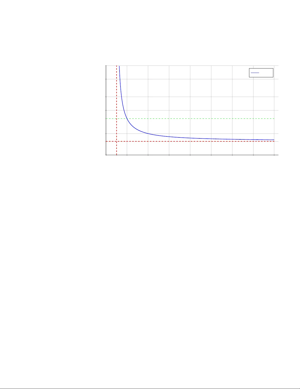
A conjecture on a tigh t norm inequalit y in the finite-dimensional l p A. S. Holev o, A. V. Utkin Steklo v Mathematical Institute, RAS, Moscow, Russia Abstract W e suggest a tigh t inequalit y for norms in d -dimensional space l p whic h has simple form ulation but app ears hard to pro ve. W e give a pro of for d = 3 and provide a detailed n umerical c heck for d ≤ 200 confirming the conjecture. W e conclude with a brief surv ey of so- lutions for kin problems which an yho w concern minimization of the output en trop y of certain quan tum c hannel and rely upon the sym- metry properties of the problem. Key words and phrases: l p -norm, R ´ en yi entrop y , tight inequalit y , maximization of a con vex function. 1 F orm ulation of the problem Quan tum information theory suggests a v ariety of optimization problems most of whic h are hard to solve analytically . F or problems suc h as computa- tion of the quantum channel capacity or accessible information the mathe- matical difficulty is finding a global maximum of a conv ex function. A single general fact is that the solution should be sough t among the extreme points of a conv ex set. No general approach exists to such problems and one should find an individual key in each sp ecial case. An example is the solution of the Gaussian optimizers conjecture for the classical capacity of bosonic Gaussian c hannels [1] (other cases will b e given in the concluding section). The prob- lem considered in the present note arose in connection with the computation 1 of accessible information for the ensem ble of “quantum pyramid” (see [3]) in [6]. Ho wev er it can b e naturally form ulated as optimization problem in d - dimensional Banach space l p without any reference to quan tum information science. Let d ≥ 3 (the case d = 2 is trivial) and consider the ( d − 1) − dimen sional h yp erplane L =  x ∈ R d : 1x ⊤ = 0 , where 1 = (1 , . . . , 1)  . We c onje ctur e the fol lowing tight ine qualities: F or α ≥ 1 ∥ x ∥ 2 α ≤ M ( d, α ) 1 / 2 α ∥ x ∥ 2 , x ∈ L ; (1) F or 0 < α < 1 ∥ x ∥ 2 α ≥ M ( d, α ) 1 / 2 α ∥ x ∥ 2 , x ∈ L, (2) wher e the c onstant M ( d, α ) is exact and is define d as fol lows: M ( d, α ) =  2 1 − α , d ≤ d ( α ); d − α  ( d − 1) α + ( d − 1) 1 − α  , d > d ( α ) (3) when α > 1 / 2 , and M ( d, α ) = 2 1 − α when α ≤ 1 / 2 (in p articular, ∥ x ∥ 1 ≥ √ 2 ∥ x ∥ 2 , x ∈ L ). Her e the value d ( α ) is the lar gest r o ot of the e quation 2 1 − α = d − α  ( d − 1) α + ( d − 1) 1 − α  . (4) In the case d ≤ d ( α ) the equalit y in the conjectured inequalities (1), (2) is attained for x 1 = − x 2 = 1 / √ 2 , x j = 0, j ≥ 3; in the case d > d ( α ) – for x 1 = q d − 1 d , x j = − q 1 ( d − 1) d , j ≥ 2 , (and for all permutations and total c hange of sign of such x j ) . F or α > 1 / 2 the equation (4) has exactly tw o roots: d = 2 and d = d ( α ) > 2 . The function d ( α ) is monotonically decreasing from + ∞ for α = 1 / 2 to d (1 ∓ 0) = 6 . 47 ... , which is the solution of the equation log( d/ 2) = d − 2 d log( d − 1) , (5) and then to d ( ∞ ) = 2 . The equation (5) is obtained b y taking the logarithmic deriv ativ e of (4) with resp ect to α at α = 1 . Another imp ortan t point is α = 2 for whic h d (2) = 3 . F or all α > 2 it holds d ( α ) < 3 , and since the dimension d 2 0 1 2 3 4 5 6 7 8 1 2 3 10 20 50 100 0 . 5 d = 2 d = 3 d (1) = 6 . 47 . . . α d (logarithmic scale) d ( α ) Figure 1: The largest ro ot d ( α ) of equation d − α  ( d − 1) α + ( d − 1) 1 − α  = 2 1 − α . tak es only integer v alues 3 , 4 , . . . , the quantit y M ( d, α ) is then alw ays given b y the second option in (3). The plot of the function α → d ( α ) , α > 0 , is giv en in Fig. 1. The pro of of the conjectured inequalities reduces to the follo wing problem: F or d ≥ 3 and α ≥ 1 show that M ( d, α ) = max x d X j =1 | x j | 2 α (6) under the c onstr aints d X j =1 | x j | 2 = 1 , d X j =1 x j = 0 , (7) with the maximizers describ e d ab ove. F or α < 1 the maximum in (6) is r eplac e d by the minimum. F or x ∈ R d with ∥ x ∥ 2 = 1 in tro duce the probability distribution P x =  | x 1 | 2 , . . . , | x d | 2  . Then for α  = 1 the problem can be reformulated in terms 3 of α -R´ en yi en tropy H α ( P x ) = (1 − α ) − 1 log P d j =1 | x j | 2 α : min x ∈ L H α ( P x ) =  log 2 , d ≤ d ( α ); (1 − α ) − 1 log d − α  ( d − 1) α + ( d − 1) 1 − α  , d > d ( α ) The case α → 1 corresp onds to minimization of the Shannon entrop y H ( P x ) considered in [6] in connection with the problem of accessible information for ensem ble of “quantum pyramid” [3]. Going to the limit and taking in to accoun t that 6 < d (1 ± 0) < 7 amounts to min x ∈ L H ( P x ) =  log 2 , d ≤ 6; log d − d − 2 d log( d − 1) , d ≥ 7 . 2 Results for d = 3 Let us first fo cus on the case α > 1. Then the v alue α = 2 is of sp ecial im- p ortance since 3 = d (2) . The hypothesis is that for 1 < α < 2 the maximum M (3 , α ) = 2 1 − α is attained on (p erm utations of )  1 / √ 2 , − 1 / √ 2 , 0  and for α > 2 , the maxim um M (3 , α ) = 3 − α (2 α + 2 1 − α ) is attained on (permuta- tions and total c hange of sign of )  p 2 / 3 , − 1 / √ 6 , − 1 / √ 6  . The transition for α = 2 b et w een the t w o regimes is rather remark able, namely: F or all x = ( x 1 , x 2 , x 3 ) satisfying x 2 1 + x 2 2 + x 2 3 = 1 , x 1 + x 2 + x 3 = 0 (8) it holds x 4 1 + x 4 2 + x 4 3 ≡ 1 2 = M (3 , 2) . Lemma. F or x satisfying (8) ther e is an angle φ such that x j = p 2 / 3 cos  φ + 2 π ( j − 1) 3  , j = 1 , 2 , 3 . (9) Note: φ = π 6 corresp onds to the maximizer  1 / √ 2 , − 1 / √ 2 , 0  , φ = 0 corresp onds to  p 2 / 3 , − 1 / √ 6 , − 1 / √ 6  . Pr o of . The conditions (8) mean that x is a unit v ector in the plane L = { x : x 1 + x 2 + x 3 = 0 } . Denote by e j the coordinate orts, ˆ e j their pro jections on to the plane L, then ˆ e 1 = (2 / 3 , − 1 / 3 , − 1 / 3) etc. with ∥ ˆ e j ∥ = p 2 / 3 and x j = e j x ⊤ = ˆ e j x ⊤ = p 2 / 3 cos φ j , j = 1 , 2 , 3 , 4 where φ j is the angle b et ween the vectors x and ˆ e j in the plane L. The angle b et w een an y t w o differen t v ectors ˆ e j is 2 π/ 3 b ecause ˆ e j ˆ e ⊤ k = − 1 2 ∥ ˆ e j ∥ ∥ ˆ e k ∥ . Therefore φ j = φ + 2 π ( j − 1) 3 , j = 1 , 2 , 3 , th us we come to (9). Then (8) b ecome 2 X j =0 cos  φ + 2 π j 3  = 0 (10) 2 3 2 X j =0 cos 2  φ + 2 π j 3  = 1 (11) and 3 X j =1 x 4 j = 4 9 2 X j =0 cos 4  φ + 2 π j 3  = 1 9 2 X j =0  1 + cos  2 φ + 4 π j 3  2 = 1 2 , where w e used (10), (11) with the doubled argument of cosine (see also (12) b elo w). Theorem. F or 1 < α < 2 the maximum M (3 , α ) = 2 1 − α is attaine d on (p ermutations of )  1 / √ 2 , − 1 / √ 2 , 0  i.e. φ = π 6 . F or α > 2 the maximum M (3 , α ) = 3 − α (2 α + 2 1 − α ) is attaine d on (p ermutations of )  p 2 / 3 , − 1 / √ 6 , − 1 / √ 6  i.e. φ = 0 . F or 0 < α < 1 the minimum M (3 , α ) = 2 1 − α is attaine d on (p ermutations of )  1 / √ 2 , − 1 / √ 2 , 0  . Pr o of. F or 0 < α < 2 w e follo w the metho d of [9] corresp onding to the case α → 1. With the aid of the Euler formula and the sum of geometric progression, one has (in our case m = 3): cos  ϕ + L 4 π j m  ≡ Re e iϕ 1 m m − 1 X j =0 exp  iL 4 π j m  =  cos ϕ, 2 L m in teger 0 otherwise , (12) where bar denotes a veraging o ver the v alues of j . 5 W e first consider the case 1 < ˙ α < 2 and the maxim um of M ( φ ) = 3 X j =1 | x j | 2 α =  2 3  α 2 X j =0     cos  φ + 2 π j 3      2 α = 3 1 − α  1 + cos  2 φ + 4 π j 3  α . F or ∥ ξ ∥ ≤ 1 w e hav e (1 + ξ ) α = 1 + α ξ + ∞ X n =2  α n  ξ n (13) = 1 + α ξ + ∞ X n =1 c 2 n ξ 2 n − ∞ X n =1 c 2 n +1 ξ 2 n +1 , where c 2 n =  α 2 n  , c 2 n +1 = −  α 2 n +1  are all p ositive for 1 < α < 2 . Th us taking in to accoun t (10) M ( φ ) = 3 1 − α [1 + α cos  2 φ + 4 π j 3  + ∞ X n =1 c 2 n cos  2 φ + 4 π j 3  2 n − ∞ X n =1 c 2 n +1 cos  2 φ + 4 π j 3  2 n +1 ] = 3 1 − α " 1 + ∞ X n =1 c 2 n cos  2 φ + 4 π j 3  2 n − ∞ X n =1 c 2 n +1 cos  2 φ + 4 π j 3  2 n +1 # . By using the form ulas for the p ow ers of the cosines (see [2], n.1.320), cos  2 φ + 4 π j 3  2 n = 1 2 2 n − 1 ( 1 2  2 n n  + n X l =1  2 n n − l  cos  2 l  2 φ + 4 π j 3  ) (14) cos  2 φ + 4 π j 3  2 n +1 = 1 2 2 n ( n X l =0  2 n + 1 n − l  cos  (2 l + 1)  2 φ + 4 π j 3  ) (15) Then the av eraging formula (12) implies M ( φ ) = ∞ X l =0 [˜ c 2 l cos (2 l ) 2 φ − ˜ c 2 l +1 cos (2 l + 1) 2 φ ] , (16) 6 where all tilted co efficients are nonnegativ e. The maximal v alue of M ( φ ) is attained if cos (2 l ) 2 φ = 1 , cos (2 l + 1) 2 φ = − 1 , i.e φ = π 2 . On the contrary , in the case 0 < α < 1 the tilted coefficients are non- p ositiv e. Then the minimal v alue of M ( φ ) is attained when cos (2 l ) 2 φ = 1 , cos (2 l + 1) 2 φ = − 1 , i.e φ = π 2 . The function M ( φ ) has p erio d π 3 , it is ev en with resp ect to φ = 0 and φ = π 6 , therefore the v alue φ = π 2 corresp onds to π 6 = π 2 − π 3 . In the case of integer α > 2 the p o w er expansion (13) has finite n umber of terms with all co efficients p ositiv e. Th us instead of (16) we obtain M ( φ ) = α X l =0 ˜ c ′ l cos 2 φl , with p ositive co efficien ts. This expression is maximized for φ = 0 . Rather surprisingly , this approac h do es not ha v e a simple extension to the case of noninteger α > 2. Due to p erio dicit y and evenness, it is sufficien t to study the b ehavior of M ( φ ) on the segmen t [0 , π 6 ]. In the Appendix, w e giv e the F ourier expansion of the function M ( φ ). Numerical study suggests that for α > 2 − M ′ ( φ ) / sin 6 φ ≥ C ( α ) > 0 , φ ∈ h 0 , π 6 i , hence M ( φ ) is decreasing and the maxim um is attained for φ = 0 . T o pro ve the h yp othesis for α > 2 it would b e sufficient to pro v e M ′ ( φ ) ≤ 0 on (0 , π 6 ). Instead w e give a proof using completely differen t approach. It is sufficient to show that for α > 2 the conditions (8) imply x 2 α 1 + x 2 α 2 + x 2 α 3 ≤ 3 − α  2 α + 2 1 − α  . Without loss of generalit y , assume that x 2 ≤ x 1 ≤ 0 ≤ x 3 = − ( x 1 + x 2 ). By introducing the v ariable x = x 1 − x 2 x 1 + x 2 ∈ [0 , 1] and using 1 + x 2 3 = 4 3 x 2 1 + x 2 2 + x 1 x 2 ( x 1 + x 2 ) 2 = 2 3 x 2 1 + x 2 2 + x 2 3 ( x 1 + x 2 ) 2 = 2 / 3 ( x 1 + x 2 ) 2 , one obtains (1 + x ) 2 + (1 − x ) 2 + 4 α ≤ 2 2 α 1 3 α  2 α + 2 1 − α  3 2 (1 + x 2 / 3)  α = (4 α + 2)  1 + x 2 3  α , 7 or g α ( x ) ≤ 4 α + 2 (17) for all x ∈ [0 , 1], where g α ( x ) = (1 + x ) 2 α + (1 − x ) 2 α − 2 (1 + x 2 3 ) α − 1 (18) is a nonnegativ e function defined on the segment [0 , 1]. The v alue g α (1) is equal to 4 α − 2 (4 / 3) α − 1 . Since (4 α + 2)((4 / 3) α − 1) − (4 α − 2) = (4 2 α − 4 α +1 ) / 3 > 0 , α > 2 , (19) g α ( x ) satisfies the inequality (17) on the righ t end of [0 , 1]. Let us prov e that g α ( x ) is monotonically increasing on [0 , 1]. Observ ation. Let a ( x ) , b ( x ) b e twice differentiable functions for x ≥ 0 suc h that a (0) = b (0) = 0; b ( x )  = 0 , x > 0 . Then  a ( x ) b ( x )  ′ = b ′ ( x ) R x 0  a ′ ( y ) b ′ ( y )  ′ b ( y ) dy b ( x ) 2 . Consequen tly , if b ( x ) and a ′ ( x ) b ′ ( x ) are increasing, then a ( x ) b ( x ) is increasing. Pr o of: Direct c heck in tegrating b y parts. Applying this observ ation to g α ( x ) with a ( x ) = (1 + x ) 2 α + (1 − x ) 2 α − 2 , b ( x ) = (1 + x 2 3 ) α − 1 , it suffices to prov e that the function [(1+ x ) 2 α +(1 − x ) 2 α ] ′ [(1+ x 2 / 3) α ] ′ is increasing, and then, by using the same observ ation, it is sufficien t to pro v e that u ( x ) := [(1 + x ) 2 α + (1 − x ) 2 α ] ′′ [(1 + x 2 / 3) α ] ′′ = 3(2 α − 1) (1 + x ) 2( α − 1) + (1 − x ) 2( α − 1) (1 + x 2 / 3) ( α − 2) (1 + (2 α − 1) x 2 / 3) is increasing. W e ha v e u ( x ) = 3(2 α − 1) u 1 ( x ) u 2 ( x ), where 1. u 1 ( x ) = (1+ x ) 2( α − 1) +(1 − x ) 2( α − 1) ((1+ x ) 2 +(1 − x ) 2 ) α − 1 ; 2. u 2 ( x ) = ((1+ x ) 2 +(1 − x ) 2 ) α − 1 (1+ x 2 / 3) ( α − 2) (1+( α − 1) x 2 / 3) . 8 By making a monotonically increasing smooth substitution t =  1+ x 1 − x  2 , t ∈ [1 , + ∞ ), the first factor u 1 ( x ) transforms into 1+ t α − 1 (1+ t ) α − 1 . Since the deriv ativ e of this expression with resp ect to t equals ( α − 1) t α − 2 − 1 (1+ t ) α and is nonnegativ e for α ≥ 2, the function u 1 ( x ) is increasing in x ∈ [0 , 1] (as a comp osition of increasing functions). The logarithmic deriv ative of u 2 ( x ) is (ln u 2 ( x )) ′ = 2 x  α − 1 1 + x 2 − α − 2 3 + x 2 − 2 α − 1 3 + (2 α − 1) x 2  = 8 x 3 ( α − 1)( α − 2) (1 + x 2 )(3 + x 2 )(3 + (2 α − 1) x 2 ) , whic h is also nonnegativ e. Hence, u 2 ( x ) is non-decreasing as well. Hence u ( x ) = 3(2 α − 1) u 1 ( x ) u 2 ( x ) is increasing, and we hav e shown that g ′ α ( x ) ≥ 0 on [0 , 1], which completes the pro of. 3 Numerical v erification Theoretical bac kground. W e consider b oth cases α > 1 and 0 < α < 1. The Lagrange metho d is useful to make the computation faster, since the constrain ts (8) yield O ( d 2 ) one-dimensional optimization problems in certain dimension d . The necessary condition for the p oin t x to b e a critical p oin t of the Lagrange function L ( x , λ ) = d X j =1 | x j | 2 α − λ ( ∥ x ∥ 2 2 − 1) − µ (1 x T ) is ∂ L ∂ x j ( x ) = 2 αx j | x j | 2( α − 1) − 2 λx j − µ = 0 , ∀ : 1 ≤ j ≤ d. Th us all the co ordinates of x satisfy the equation 2 αx | x | 2( α − 1) − 2 λx − µ = 0 (20) for some real λ and µ , which has at most 3 solutions. Indeed, the deriv ativ e of the left hand side of (20) m ultiplied by (1 − α ) 4 α ( α − 1) 2 | x | 2( α − 1) − 2 λ ( α − 1) (21) 9 is either nonnegative ev erywhere or negativ e on an interv al. This means that, up to p erm utation and sign changes, maximizer has the form x = ( s 0 , ..., s 0 | {z } k 0 times , s 1 , ..., s 1 | {z } k 1 times , s 2 , ..., s 2 | {z } k 2 times ) , s 0 ≤ 0 ≤ s 1 ≤ s 2 . (22) T o construct a one-dimensional parametrization put s 0 = − ( k 1 s 1 + k 2 s 2 ) /k 0 in to the quadratic form q ( s 1 , s 2 ) = k 0 s 2 0 ( s 1 , s 2 ) + k 1 s 2 1 + k 2 s 2 2 and find a linear transformation  s 1 s 2  =  u 1 u 2 v 1 v 2   c 1 c 2  (23) suc h that q ( s 1 ( c 1 , c 2 ) , s 2 ( c 1 , c 2 )) = λ 1 c 2 1 + λ 2 c 2 2 . The parameters u 1 , u 2 , v 1 , v 2 can b e calculated as follows: 1. Find co efficients A, B , C of the form q ( s 1 , s 2 ) = As 2 1 + 2 B s 1 s 2 + C s 2 2 . A = k 1 ( k 1 + k 0 ) k 0 B = k 1 k 2 k 0 C = k 2 ( k 2 + k 0 ) k 0 ; 2. Compute λ 1 , 2 = k 0 ( k 1 + k 2 ) + k 2 1 + k 2 2 ± √ D 2 k 0 , where D = ( k 0 ( k 1 + k 2 ) + k 2 1 + k 2 2 ) 2 − 4 k 0 k 1 k 2 d ; 3. Express u 1 = B p B 2 + ( A − λ 1 ) 2 , v 1 = λ 1 − A p B 2 + ( A − λ 1 ) 2 and u 2 = − v 1 , v 2 = u 1 . 4. Then w e find s 1 = u 1 c 1 + u 2 c 2 , s 2 = v 1 c 1 + v 2 c 2 . 10 Therefore, the set of pairs ( s 1 , s 2 ) with condition q ( s 1 , s 2 ) = 1 is parametrized b y t ∈ [0 , 2 π ) according to the formula  s 1 ( t ) s 2 ( t )  =  u 1 u 2 v 1 v 2  cos( t ) √ λ 1 sin( t ) √ λ 2 ! (24) Th us, when the maximizer of F α ( x ) = d P j =1 | x j | 2 α for α > 1 (or the min- imizer for α ∈ (0 , 1)) has non-zero co ordinates, these co ordinates must b e equal to one of the follo wing real num b ers – s 0 , s 1 or s 2 with mul- tiplicities k 0 , k 1 and k 2 = d − k 0 − k 1 – the maxim um M ( d, α ) can b e found numerically b y considering the function of one v ariable f d,α ; k 1 ,k 2 ( t ) = k 0  k 1 s 1 ( t )+ k 2 s 2 ( t ) k 0  2 α + k 1 s 1 ( t ) + k 2 s 2 ( t ). Numerical v erification algorithm. W e consider the maximization prob- lem for the function F α ( x ) = d X j =1 | x j | 2 α , α > 1 , under the constraints ∥ x ∥ 2 2 = d X j =1 x 2 j = 1 , d X j =1 x j = 0 . 11 Algorithm 1 Numerical v erification of the maximization h yp othesis for F α 1: Input: Parameter α > 1, dimension range [ d min , d max ], tolerance ϵ = 10 − 8 2: Output: V erification result for eac h dimension d 3: pro cedure VerifyHypothesis ( α , d min , d max ) 4: for d = d min to d max do 5: ▷ Compute theoretical bounds 6: M 1 ( α, d ) ← d − α  ( d − 1) α + ( d − 1) 1 − α  7: M 2 ( α, d ) ← 2 1 − α 8: M num ( α, d ) ← 0 9: for all ordered triples ( k 0 , k 1 , k 2 ) with k 0 + k 1 + k 2 = d , k 0 ≥ 1, k 1 ≤ k 2 do 10: ▷ Compute parametrization s 0 ( t ) , s 1 ( t ) , s 2 ( t ) as in P aragraph 3 11: ( s 0 ( t ) , s 1 ( t ) , s 2 ( t )) ← P arametrization( k 0 , k 1 , k 2 ) 12: ▷ Maximize one-dimensional function 13: f ( t ) ← k 0 | s 0 ( t ) | 2 α + k 1 | s 1 ( t ) | 2 α + k 2 | s 2 ( t ) | 2 α 14: M cand ← max t ∈ [0 , 2 π ) f ( t ) 15: if M cand > M num ( α, d ) then 16: M num ( α, d ) ← M cand 17: end if 18: end for 19: ▷ T est hypotheses 20: ∆ 1 ← | M num ( α, d ) − M 1 ( α, d ) | 21: ∆ 2 ← | M num ( α, d ) − M 2 ( α, d ) | 22: v alid 1 ← (∆ 1 ≤ ϵ ) 23: v alid 2 ← (∆ 2 ≤ ϵ ) 24: ▷ Accept hypothesis if either b ound matc hes 25: confirmed ← v alid 1 or v alid 2 26: Output result for dimension d 27: end for 28: end pro cedure F or the n umerical v erification of hypothesis (2) (with α ∈ (0 , 1)), the algorithm description should in volv e finding the minim um of the function f ( t ) from the algorithm instead of its maxim um. 12 Complexit y . Instead of optimizing ov er R d , the algorithm reduces the problem to O ( d 2 ) one-dimensional optimizations, making v erification feasible for d up to sev eral h undred. Exp ected outcome. The b ehavior of M num ( d ) dep ends on α as follows: • F or α > 1: there exists a critical dimension d ( α ) suc h that M num ( d ) ≈ ( 2 1 − α , d < d ( α ) d − α  ( d − 1) α + ( d − 1) 1 − α  , d ≥ d ( α ) • F or 0 . 5 < α < 1: the b eha vior is reversed, i.e., M num ( d ) ≈ ( d − α  ( d − 1) α + ( d − 1) 1 − α  , d < d ( α ) 2 1 − α , d ≥ d ( α ) • F or 0 < α ≤ 0 . 5: M num ( d ) ≈ 2 1 − α for all d . The critical dimension satisfies (5) 2 1 − α = d ( α ) − α  ( d ( α ) − 1) α + ( d ( α ) − 1) 1 − α  . V erification results. The algorithm confirms the hypothesis for all tested dimensions within tolerance ϵ , sho wing p erfect agreemen t with the theoretical predictions. Sp ecifically , n umerical verification was p erformed for α = 0 . 05, 0 . 2, 0 . 45, 0 . 5, 0 . 55, 0 . 7, 0 . 95, 1 . 01, 1 . 1, 1 . 5, and 2 across dimensions d = 3 through 200. In each case, the computed maxim um M num ( d, α ) coincides (within the prescrib ed tolerance) with the conjectured v alue. The corre- sp ondence holds for ev ery tested pair ( α, d ), confirming the v alidity of the structural hypothesis ov er the in vestigated range. 4 Discussion Here w e giv e references to solutions of sev eral problems akin to our con- jecture. All cases concern minimization of the output en tropy of certain quan tum c hannel (normalized completely positive map) and rely upon the symmetry prop erties of the problem. 13 In [7] Lieb gav e a solution of the W ehrl conjecture which can b e reformu- lated as a conjecture ab out the minimal output en trop y of the measurement (quan tum-classical) c hannel asso ciated with the Glauber’s coheren t states with the underlying Heisen b erg group, and generalized the conjecture to SU(2) group. The solution w as based on the tigh t v ersions of Y oung’s and Hausdorff-Y oung inequalities in the classical harmonic analysis. In [8] Lieb and Solov ej prov ed the W ehrl-t yp e en tropy conjecture for symmetric SU(N) coheren t states and suggested a similar conjecture for a large class of Lie groups and their representation. In the pap ers of Holev o [4] and Holevo and Filipp o v [5] the Gaussian optimizers conjecture was prov ed for the classical capacit y of Gaussian measuremen t c hannels by using generalizations of the logarithmic Sob olev inequalit y . W e surmise that the h yp othesis of the present pap er could be regarded as a discrete relativ e of the aforemen tioned problems, with the harmonic analysis of the p ermutation group and its represen tation b y the symmetry group of d − 1-dimensional simplex as a p ossible to ol (cf. the first part of the pro of of our Theorem for the case d = 3). App endix By using the expansions (14), (15) with the interc hanged summation order and the av eraging formula (12) one can obtain the F ourier expansion M ( φ ) = 3 1 − α " 1 + C 0 ( α ) + ∞ X k =1 cos 6 k φ ∞ X n =0 α ( α − 1) . . . ( α − 2 n − 3 k + 1) n !( n + 3 k )! 2 − (2 n +3 k − 1) # , (25) where C 0 ( α ) = P ∞ n =1 α ( α − 1) ... ( α − 2 n +1) ( n !) 2 2 − 2 n . Pr o of . Inserting (14), (15) in to the expansion (13), we obtain 3 α − 1 M ( φ ) = 1 + P ∞ n =1  α 2 n  1 2 2 n − 1 n 1 2  2 n n  + P n l =1  2 n n − l  cos  2 l  2 φ + 4 π j 3  o + P ∞ n =1  α 2 n +1  1 2 2 n P n l =1  2 n +1 n − l  cos  (2 l + 1)  2 φ + 4 π j 3  = 1 + C 0 ( α ) + P ∞ n =1 P n l =1 α ( α − 1) ... ( α − 2 n +1) ( n − l )!( n + l )! 2 − (2 n − 1) cos  2 l  2 φ + 4 π j 3  + P ∞ n =1 P n l =0 α ( α − 1) ... ( α − 2 n ) ( n − l )!( n + l +1)! 2 − 2 n cos  (2 l + 1)  2 φ + 4 π j 3  = 1 + C 0 ( α ) + P ∞ l =1 cos  2 l  2 φ + 4 π j 3  P ∞ n = l α ( α − 1) ... ( α − 2 n +1) ( n − l )!( n + l )! 2 − (2 n − 1) + P ∞ l =0 cos  (2 l + 1)  2 φ + 4 π j 3  P ∞ n = l α ( α − 1) ... ( α − 2 n ) ( n − l )!( n + l +1)! 2 − 2 n 14 In the last sum the term with l = 0 v anishes due to (12) and in tro ducing n ′ = n − l w e obtain 1 + C 0 ( α ) + ∞ X l =1 cos  2 l  2 φ + 4 π j 3  ∞ X n ′ =0 α ( α − 1) . . . ( α − 2 n ′ − 2 l + 1) ( n ′ )!( n ′ + 2 l )! 2 − (2 n ′ +2 l − 1) + ∞ X l =1 cos  (2 l + 1)  2 φ + 4 π j 3  ∞ X n ′ =0 α ( α − 1) . . . ( α − 2 n ′ − 2 l ) ( n ′ )!( n ′ + 2 l + 1)! 2 − (2 n +2 l ) = 1 + C 0 ( α ) + ∞ X L =1 cos  L  2 φ + 4 π j 3  ∞ X n ′ =0 α ( α − 1) . . . ( α − 2 n ′ − L + 1) ( n ′ )!( n ′ + L )! 2 − (2 n ′ + L − 1) Due to (12), only terms corresp onding to L = 3 k , k = 1 , 2 , ... survive, hence (25) follows. References [1] V. Gio v annetti, A. S. Holevo, R. Garcia-P atron, A solution of Gaussian optimizer conjecture for quan tum channels, Commun. Math. Ph ys. 334 :3, 1553-1571 (2015). [2] I.S. Gradsh teyn and I.M. Ryzhik, T able of In tegrals, Series, and Pro ducts Sev enth Edition, 2007, Elsevier Inc. [3] B.-G. Englert and J. ˇ Reh´ a ˇ cek, How well can y ou kno w the edge of a quan tum p yramid, J. Mo d. Optics 57 N3 (2010) 218-226. [4] A. S. Holev o, “Logarithmic Sobolev inequalit y and Hyp othesis of Quan- tum Gaussian Maximizers”, Russian Math. Surv eys, 77 :4, 766-768 (2022). [5] A. S. Holev o, S. N. Filippov, “Quan tum Gaussian maximizers and log- Sob olev inequalities”, Lett. Math. Phys., 113 , 10, (2023). [6] A.S. Holev o, A.V. Utkin, Quantum accessible information and classical en tropy inequalities. [7] Lieb, E.H. Pro of of an entrop y conjecture of W ehrl. Commun. Math. Ph ys. 62 , 35–41 (1978). 15 [8] Lieb, E.H., Solov ej, Pro of of the W ehrl-type entrop y conjecture for sym- metric SU(N) coherent states. Arxiv: 1506.07633. [9] M. Sasaki, S. M. Barnett, R. Jozsa, M. Osaki, and O. Hirota, Accessible information and optimal strategies for real symmetrical quan tum sources, Ph ys. Rev. A 59 (1999) 3325-3335. arXiv:quant-ph/9812062 16