Microergodicity implies orthogonality of Matérn fields on bounded domains in $\mathbb{R}^4$

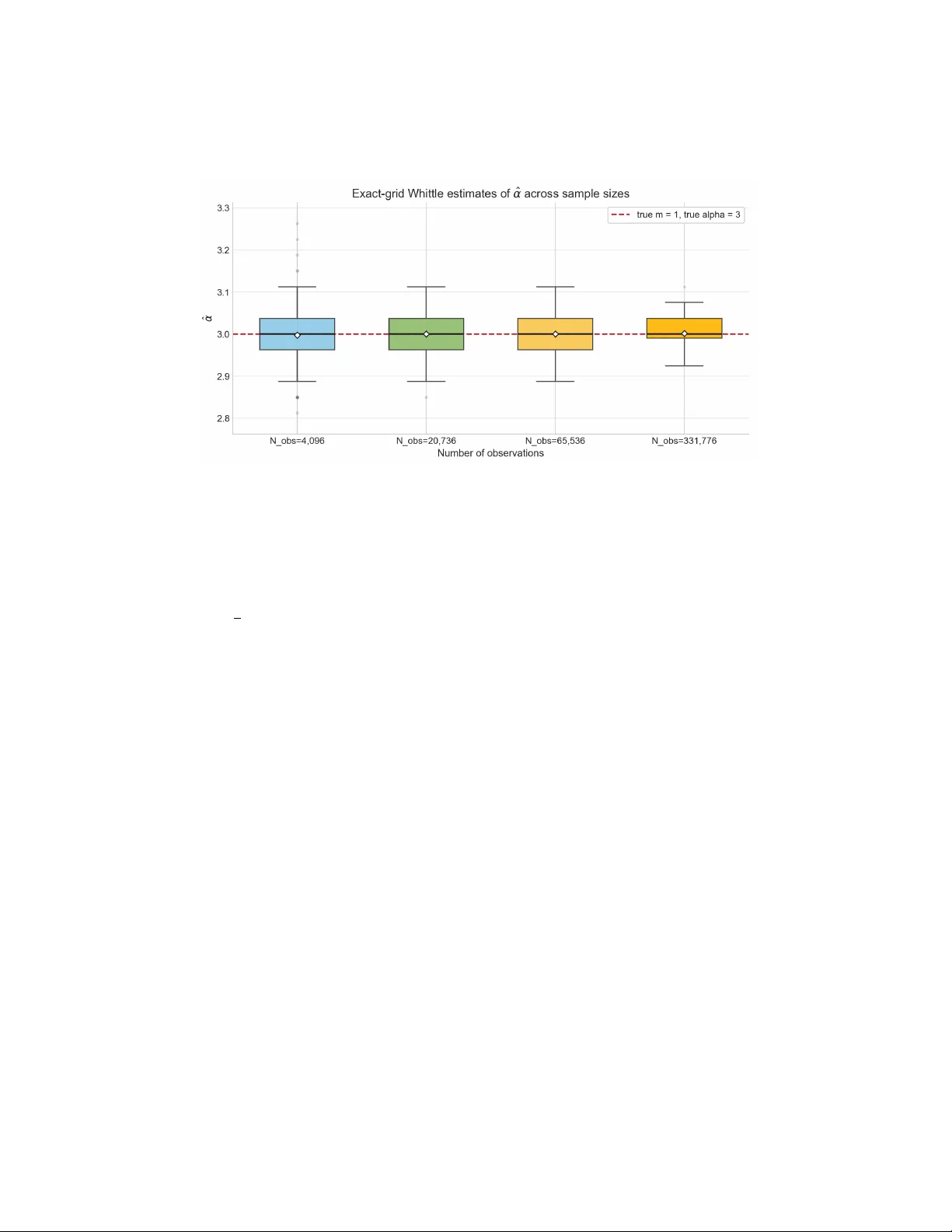
MICR OERGODICITY IMPLIES OR THOGON ALITY OF MA T ´ ERN FIELDS ON BOUNDED DOMAINS IN R 4 N A TESH S. PILLAI A B S T R AC T . Mat ´ ern random fields are one of the most widely used classes of models in spatial statistics. The fixed-domain identifiability of covariance pa- rameters for stationary Mat ´ ern Gaussian random fields exhibits a dimension- dependent phase transition. For known smoothness ν , Zhang [ 1 ] showed that when d ≤ 3 , two Mat ´ ern models with the same microergodic parameter m = σ 2 α 2 ν induce equiv alent Gaussian measures on bounded domains, while An- deres [ 2 ] proved that when d > 4 , the corresponding measures are mutually singular whenev er the parameters differ . The critical case d = 4 for stationary Mat ´ ern models has remained open. W e resolv e this case. Let d = 4 and consider two stationary Mat ´ ern models on R 4 with parameters ( σ 1 , α 1 ) and ( σ 2 , α 2 ) satisfying σ 2 1 α 2 ν 1 = σ 2 2 α 2 ν 2 , α 1  = α 2 . W e prov e that the corresponding Gaussian measures on any bounded observ ation domain are mutually singular on e very countable dense observation set, and on the associated path space of continuous functions. Our approach can be viewed as a spectral analogue of the higher-order incre- ment method of Anderes [ 2 ]. Whereas Anderes isolates the second irregular co- variance coef ficient through renormalized quadratic variations in physical space, we detect the first non vanishing high-frequency spectral mismatch via localized Fourier coefficients and use a normalized Whittle score to identify parameters. More broadly , the localized spectral probing framework used here for detect- ing subtle covariance differences in Gaussian random fields may be useful for studying identifiability and estimation in other spatial models. 1. I N T R O D U C T I O N Gaussian random fields are a central tool for modeling spatial dependence [ 3 , 4 ]. Let Y = { Y ( t ) : t ∈ R d } be a mean-zero stationary Gaussian field with cov ariance Co v( Y ( s ) , Y ( t )) = K ( t − s ) . Many spatial models further assume isotropy , meaning that there exists a function φ : [0 , ∞ ) → R such that K ( h ) = φ ( | h | ) , h ∈ R d . 2020 Mathematics Subject Classification. Primary 60G60; Secondary 62M30, 62M40. K e y wor ds and phrases. Mat ´ ern class, Gaussian random fields, infill asymptotics, spectral smoothing, localization. 1 2 N A TESH S. PILLAI Among stationary isotropic cov ariance families, the Mat ´ ern class occupies a dis- tinguished position. For variance parameter σ 2 > 0 , range parameter α > 0 , and smoothness param- eter ν > 0 , the Mat ´ ern cov ariance function is [ 3 ] K ( h ) = σ 2 ( α | h | ) ν 2 ν − 1 Γ( ν ) K ν ( α | h | ) , h ∈ R d , (1) where K ν is the modified Bessel function of the second kind, and K (0) = σ 2 by continuity . The parameter σ 2 sets the marginal variance, α governs the spatial scale of dependence, and ν controls regularity . Larger values of ν correspond to smoother fields; in particular , the Mat ´ ern model provides a continuous hierarchy ranging from rough fields (for example the exponential model when ν = 1 2 ) to v ery smooth ones, and after suitable rescaling it approaches the squared e xponential kernel as ν → ∞ . The survey [ 5 ] giv es a panoramic overvie w of the multifaceted use of the Mat ´ ern family in statistical applications and be yond. For stationary fields it is often more conv enient to work in the spectral domain. By Bochner’ s theorem, K ( h ) = 1 (2 π ) d Z R d e iξ · h f ( ξ ) dξ , where f is the spectral density . For the Mat ´ ern cov ariance ( 1 ), the spectral density is [ 3 , p. 49] f σ,α,ν ( ξ ) = C d,ν σ 2 α 2 ν ( α 2 + | ξ | 2 ) − ( ν + d/ 2) , ξ ∈ R d , (2) for a constant C d,ν > 0 depending only on d and ν . Hence, as | ξ | → ∞ , f ( ξ ) ∼ C σ 2 α 2 ν | ξ | − 2 ν − d , | ξ | → ∞ . (3) This high-frequency tail is fundamental for fixed-domain asymptotics. It shows, first, that ν determines the spectral decay and therefore the local regularity of the field. Second, it identifies the combination m = m ( σ, α ) := σ 2 α 2 ν (4) as the leading coefficient in the spectral tail. In the parameterization used in this paper , this is the micr oer godic parameter [ 3 ]. 1.1. Fixed-domain asymptotics and microergodicity . In spatial statistics one of- ten observes a random field on a fixed bounded domain while the sampling design becomes increasingly dense. This is the fixed-domain , or infill , asymptotic regime. Since the data arise from a single realization of a Gaussian random field, an im- portant issue for statistical inference is not merely whether different parameter v alues induce dif ferent Gaussian measures, but whether the corresponding mea- sures are equiv alent or mutually singular on the observation sigma-field. Under fixed-domain asymptotics, this distinction governs which cov ariance features are consistently estimable from dense observ ations of a single path. The present paper studies this issue for stationary Mat ´ ern fields on Euclidean domains and asks which cov ariance parameters are identifiable, and therefore es- timable, in the fixed-domain asymptotic regime. For the Mat ´ ern family with known OR THOGONALITY OF MA T ´ ERN FIELDS ON BOUNDED DOMAINS IN R 4 3 smoothness ν , the leading spectral asymptotics already suggest what should hap- pen. T wo models with the same v alue of m = m ( σ, α ) := σ 2 α 2 ν hav e the same high-frequency tail to first order . This makes m ( σ, α ) the natural estimable combination under infill asymptotics, while the separate identifiability of σ 2 and α depends on whether the next-order information in the covariance or the spectrum can also be recov ered from dense data. A seminal result of Zhang [ 1 ] shows that when d ≤ 3 , two stationary Mat ´ ern fields with the same smoothness ν and the same microer godic parameter m in- duce equivalent Gaussian measures on e very bounded domain. In these dimen- sions the variance and range parameters cannot be separated consistently from a single dense realization. At the opposite end, Anderes [ 2 ] proved that when d > 4 , the corresponding Mat ´ ern measures are orthogonal whenever the parameters dif fer . Equi valently , variance and range can be consistently separated in that regime. For stationary Mat ´ ern fields on R d , the d = 4 case has remained open until no w . Dimension four turns out to be the critical case. When two Mat ´ ern models hav e the same microergodic parameter m and smoothness ν but dif ferent range parameters α , the discrepancy between their cov ariance structures lies exactly at the boundary between summable and non-summable second–order effects across frequencies. In lower dimensions the cumulativ e discrepancy remains bounded, while in higher dimensions it grows at a polynomial rate. In dimension four the ac- cumulation is much slower: the distinguishing signal grows only log arithmically as higher frequencies are incorporated. As we sho w below , this slow but unbounded accumulation is precisely what makes the four–dimensional case identifiable. Re- cent work on related Gaussian field models has continued to identify dimension four as the delicate boundary case in the Euclidean setting [ 5 – 7 ]. 1.2. Our contribution. W e settle the remaining Euclidean case for d = 4 . W e prov e in Theorem 1 that in dimension d = 4 , two stationary Mat ´ ern fields with the same smoothness parameter and the same microer godic parameter , but with dif ferent range parameters, induce mutually singular Gaussian measures on every countable dense observation set in a bounded domain. W e pro ve this by first sho w- ing that the associated la ws on path space are mutually singular and then projecting to dense sets. More precisely , let Y 1 and Y 2 be stationary Mat ´ ern fields on R 4 with parameters ( σ 1 , α 1 ) and ( σ 2 , α 2 ) and common smoothness ν > 0 . Assume σ 2 1 α 2 ν 1 = σ 2 2 α 2 ν 2 , α 1  = α 2 . (5) Then Theorem 1 shows that the induced Gaussian measures on an y countable dense observ ation set are mutually singular . Thus, unlike the case d ≤ 3 , the range parameter is asymptotically distinguishable from dense fixed-domain data for d = 4 . 4 N A TESH S. PILLAI 1.3. Idea of the proof. Our ke y idea is to probe the field using localized Fourier coef ficients, rev ealing a small variance mismatch at high frequencies whose accu- mulation produces a logarithmic signal in dimension four . Our ar gument works for any d ≥ 4 and thus also recov ers the orthogonality results for d > 4 from Anderes [ 2 ]. Let D ⊂ R 4 be a bounded domain and suppose we ha ve two Mat ´ ern laws P 1 and P 2 satisfying ( 5 ) on D . Our proof resolves the critical case d = 4 by working in the spectral domain. Writing p := ν + 2 , the Mat ´ ern spectral density in dimension four is f σ,α,ν ( ξ ) = C ν σ 2 α 2 ν ( α 2 + | ξ | 2 ) − p . Under the microergodic matching condition ( 5 ) σ 2 1 α 2 ν 1 = σ 2 2 α 2 ν 2 , α 1  = α 2 , the two spectral densities agree at leading order , f j ( ξ ) ∼ C ν m | ξ | − 2 p , | ξ | → ∞ , with m = σ 2 j α 2 ν j . The first discrepancy appears at the next order , f 2 ( ξ ) − f 1 ( ξ ) ≍ | ξ | − 2 p − 2 , f 2 ( ξ ) − f 1 ( ξ ) f 1 ( ξ ) ≍ | ξ | − 2 . In dimension four this decay is critical, since X | k |≤ N | k | − 4 ≍ log N . Thus the mismatch accumulates only logarithmically across frequencies, and this marginal di vergence is the signal e xploited in our construction. T o access this signal, we “probe” the field by constructing localized Fourier coef ficients. Fix a smooth cutoff χ ∈ C ∞ c ( D ) 1 and define X k := Z D χ ( t ) e − ik · t Y ( t ) dt, k ∈ N 4 . (6) Under the j th model, X k is a centered complex Gaussian random variable with v ariance v j ( k ) = E j | X k | 2 = (2 π ) − 4 ( f j ∗ | b χ | 2 )( k ) . Thus v j ( k ) is a local smoothing of f j ov er a frequency window of scale (diam(supp χ )) − 1 . Define the relati ve v ariance mismatch δ k = v 2 ( k ) v 1 ( k ) − 1 . (7) 1 For e xample, if B (0 , R ) ⊂ D , one may take χ ( t ) =    exp  − 1 1 − | t | 2 /R 2  , | t | < R , 0 , | t | ≥ R . OR THOGONALITY OF MA T ´ ERN FIELDS ON BOUNDED DOMAINS IN R 4 5 A direct expansion (Lemma 5 ) sho ws that δ k ∼ p ( α 2 1 − α 2 2 ) | k | − 2 . Consequently , for the shell Λ N := { k ∈ N 4 : K 0 ≤ ∥ k ∥ ∞ ≤ N } , L N := X k ∈ Λ N δ 2 k , (8) we hav e L N ≍ log N . The quantity L N turns out to be the natural information scale of the problem. T o separate models using the abo ve observ ation, we consider the normalized quadratic statistic T N = 1 L N X k ∈ Λ N δ k  | X k | 2 v 1 ( k ) − 1  . (9) Each term is centered under P 1 , while under P 2 it has mean δ k , so that E 1 [ T N ] = 0 , E 2 [ T N ] = 1 . Thus T N aggregates a sequence of weak frequency-wise signals into an order - one separation. In Section 3 we sho w that the statistic T N can be interpreted as a natural score-type statistic associated with the difference between the two localized spectral laws. A key point is that the variables { X k } are not independent. Ho wever , since the Fourier transform b χ decays rapidly , localization yields that the cov ariances E j [ X k X ℓ ] , E j [ X k X ℓ ] decay rapidly in | k − ℓ | and | k + ℓ | , respectiv ely , for j = 1 , 2 . This off-diagonal decay enables us to control the v ariance of T N and sho w that: V ar j ( T N ) ≲ L − 1 N . Since L N ≍ log N , the variance vanishes along a sparse subsequence { N s } , and we obtain almost sure separation T N s → 0 P 1 -a.s. , T N s → 1 P 2 -a.s. This yields a separating e vent and hence mutual singularity . This viewpoint may be interpreted as a spectral analogue of the increment method of Anderes [ 2 ]; see Section 3 for further details. In Anderes [ 2 ], the second irreg- ular cov ariance coefficient is isolated in physical space, whereas here we isolate the first non v anishing spectral mismatch at high frequency . The critical dimension d = 4 appears because the information scale L N di ver ges only logarithmically . More broadly , this spectral probing perspectiv e provides a systematic way to ana- lyze equi v alence and orthogonality of Gaussian measures via localized frequenc y information. It also points toward a ne w class of inference procedures, in which parameters are identified by aggreg ating weak high-frequenc y discrepancies, in the spirit of localized Whittle estimation. 6 N A TESH S. PILLAI Our construction is related to, but not identical with, tapering. Classical lag tapering [ 8 ] r eplaces the stationary cov ariance kernel K ( h ) by K tap ( h ) = K ( h ) ω χ ( h ) , ω χ ( h ) := Z R 4 χ ( u + h ) χ ( u ) du, which corresponds to replacing the spectral density f by (2 π ) − 4 ( f ∗ | b χ | 2 ) ; we do not change the cov ariance kernel. Thus, although at each freque ncy we recov er the same smoothed spectral quantity as in tapering, the off-diagonal structure induced by our spectral localization does not coincide with that of any tapered stationary cov ariance model. 1.4. Related W ork. A recent paper of Bolin and Kirchner [ 6 ] studies equiv alence of Gaussian measures for generalized Whittle–Mat ´ ern fields on a bounded domain D ⊂ R d , defined through fractional elliptic operators with homogeneous Dirichlet boundary conditions. In the classical constant-coefficient case, their model is µ = N ( m, τ − 2 L − 2 β ) , L = − ∆ + κ 2 , vie wed as a Gaussian measure on L 2 ( D ) . Here β plays the role of the smoothness index, with the usual whole-space correspondence ν = 2 β − d 2 , and κ plays the role of the range parameter . In the constant-coefficient case, the scaling parameter τ − 2 is proportional, up to a constant depending only on ( d, ν ) , to the Mat ´ ern microer godic combination σ 2 κ 2 ν . Thus their parameter τ is the bounded-domain analogue of the leading spectral scale in ( 3 ). Their Corollary 3.3 gives a complete equiv alence classification for the classical bounded-domain Whittle–Mat ´ ern model. In dimensions d ≤ 3 , equi v alence holds if and only if β = ˜ β , τ = ˜ τ , together with the corresponding Cameron–Martin condition on the means. In di- mensions d ≥ 4 , equiv alence additionally requires κ 2 = ˜ κ 2 . Therefore, in the bounded-domain classical Whittle–Mat ´ ern model, matching the leading scale is no longer sufficient in dimension 4 : once β and τ are matched, any nontrivial change in κ forces non-equiv alence. This mirrors our result for the stationary Euclidean model obtained in this paper . W e study the restriction to a bounded observation domain of a stationary Mat ´ ern field defined on all of R 4 . Thus translation inv ariance holds in the ambient Eu- clidean space and is broken only by the restriction of the observ ations to D . By contrast, the Whittle–Mat ´ ern field in [ 6 ] is constructed intrinsically on D through the Dirichlet operator L = − ∆ + κ 2 , so the boundary conditions are part of the model itself and the resulting field is generally non-stationary . Moreover , on a bounded domain the classical stationary Mat ´ ern model does not admit a fixed fractional-operator representation since its eigenfunctions depend on the smooth- ness parameter . Thus the operator-based framew ork of [ 6 ] does not directly apply . OR THOGONALITY OF MA T ´ ERN FIELDS ON BOUNDED DOMAINS IN R 4 7 In the limit as the domain expands to R d , the model con verges to the stationary Mat ´ ern field, and the same dimension-dependent equi v alence behavior is expected. At the lev el of asymptotics, howe v er , the mechanisms behind the two proofs are strikingly similar . In the constant-coefficient bounded-domain model, the Dirichlet eigenfunctions diagonalize both cov ariance operators. If ˆ λ j denotes the j th eigen- v alue of the Dirichlet Laplacian on D , then λ j = ˆ λ j + κ 2 , ˜ λ j = ˆ λ j + ˜ κ 2 , and the Feldman–H ´ ajek criterion [ 9 , Theorem 2.5] reduces to the square-summability of the diagonal ratios c j − 1 , c j =  ˜ τ τ  1 /β ˆ λ j + ˜ κ 2 ˆ λ j + κ 2 . After matching the leading scale, one has c j − 1 ∼ ( ˜ κ 2 − κ 2 ) ˆ λ − 1 j . Since W eyl’ s law gi ves ˆ λ j ≍ j 2 /d , it follo ws that ( c j − 1) 2 ≍ j − 4 /d and for d = 4 the corresponding partial sums satisfy X j ≤ N ( c j − 1) 2 ≍ X j ≤ N 1 j = log N + O (1) . Thus d = 4 is exactly the logarithmic borderline for the Feldman–H ´ ajek square- summability condition in this setting. Our proof isolates the same critical second-order mismatch in continuous fre- quency . The main dif ference lies in the proof architecture. In [ 6 ], the constant- coef ficient bounded-domain model is exactly diagonal in a common Dirichlet eigen- basis, so equiv alence can be read off from a diagonal square-summability condi- tion. In our stationary setting, we must control the off-diagonal covariances and pseudo-cov ariances introduced by localization. This is our key technical contri- bution. The connection with Feldman–H ´ ajek is through the quantity L N : in an exactly diagonal model, L N is the truncated Feldman–H ´ ajek square-summability sum, while in our localized setting it becomes the leading score/information scale on increasing finite-dimensional frequency windows. Our off-diagonal estimates sho w that this same scale continues to gov ern the true model. 1.5. Organization of the paper . Section 2 states the main theorem precisely . Sec- tion 3 places our work in the context of previous work and giv es a likelihood in- terpretation of our statistic ( 9 ). Section 4 passes from dense observations to path- space laws on C ( D ) . Sections 5–8 dev elop the localized Fourier coef ficients, es- tablish diagonal asymptotics and off-diagonal decay , and construct the separating statistic; Section 9 gi ves the proof of the main result. Section 10 gives a simulation study sho wing that an estimation procedure based on the Whittle pseudo-likelihood recov ers the parameter α . Throughout the paper , we write a ≳ b if there exists a constant C > 0 , depending only on fixed model parameters (such as d , ν , the domain D , and the cutoff χ ), such that a ≥ C b ; we write a ≍ b if both a ≳ b 8 N A TESH S. PILLAI and b ≳ a . W e use O ( · ) and o ( · ) in the usual asymptotic sense as | k | → ∞ (or N → ∞ ), with all implicit constants depending only on these fixed parameters. 2. M A I N R E S U LT Fix ν > 0 and write p := ν + 2 . Let Y j = { Y j ( t ) : t ∈ R 4 } , j = 1 , 2 , be mean-zero stationary Mat ´ ern Gaussian fields with parameters ( σ j , α j ) and common smoothness ν . Their spectral densities are f j ( ξ ) = C ν σ 2 j α 2 ν j ( α 2 j + | ξ | 2 ) − p , ξ ∈ R 4 , (10) where C ν > 0 depends only on ν and on the Fourier con vention. W e impose the microergodic matching condition σ 2 1 α 2 ν 1 = σ 2 2 α 2 ν 2 =: m, α 1  = α 2 . (11) Under ( 11 ), f j ( ξ ) = C ν m ( α 2 j + | ξ | 2 ) − p . The follo wing is our main result. Theorem 1. Let D ⊂ R 4 be a bounded domain with nonempty interior and S ⊂ D be countable and dense. Denote by P S j the law of the coor dinate pr ocess { Y j ( t ) : t ∈ S } on R S . Assume ( 11 ) . Then P S 1 ⊥ P S 2 . In particular , for the dense grid D ∞ := [ n ≥ 1 D ∩ n − 1 Z 4 , the laws of the coor dinate pr ocesses { Y j ( t ) : t ∈ D ∞ } ar e mutually singular . The proof proceeds by first establishing singularity of the induced path laws on C ( D ) and then transferring that conclusion to dense observ ation sets. 3. T H E C R I T I C A L D I M E N S I O N , A N D E R E S ’ M E T H O D , A N D O U R A P P R OA C H The mechanism behind the phase transition is already visible in the local co- v ariance expansion of the Mat ´ ern model; see Anderes [ 2 ]. Near the origin, the cov ariance admits a sequence of non-polynomial terms with leading orders | h | 2 ν and | h | 2 ν +2 (with logarithmic modifications), whose coef ficients are proportional to σ 2 α 2 ν and σ 2 α 2 ν +2 , respecti vely . The first coefficient is e xactly the microer- godic parameter σ 2 α 2 ν . Thus, if only the leading irregular term can be recov ered from the data, then one can estimate only the microergodic combination. If the next irre gular term can also be identified, then the parameters σ 2 and α can be separated. Anderes [ 2 ] makes this precise using higher-order directional increments. For a fixed nonzero direction h , define ∆ h Y ( t ) = Y ( t + h ) − Y ( t ) , ∆ ℓ h Y ( t ) = ∆ h (∆ ℓ − 1 h Y ( t )) . OR THOGONALITY OF MA T ´ ERN FIELDS ON BOUNDED DOMAINS IN R 4 9 For observ ations on the grid Ω n = Ω ∩ n − 1 Z d , he considers the quadratic v ariation statistic Q ℓ n ( h ) = 1 #Ω n X j ∈ Ω n n 2 ν  ∆ ℓ h/n Y ( j )  2 . Lemma 1 of Anderes [ 2 ] sho ws that for ℓ > ν + 1 , E  ∆ ℓ h/n Y ( t )  2 = a ℓ ν ( h ) n − 2 ν + b ℓ ν ( h ) n − 2 ν − 2 + o ( n − 2 ν − 2 ) , where a ℓ ν ( h ) is proportional to σ 2 α 2 ν and b ℓ ν ( h ) is proportional to σ 2 α 2 ν +2 . Thus Q ℓ n ( h ) consistently estimates the leading coef ficient a ℓ ν ( h ) , whose dependence on the unkno wn parameters occurs through the microergodic combination σ 2 α 2 ν . T o isolate the next-order coef ficient, Anderes compares two increment orders u  = v and considers R u,v n ( h ) = n 2  Q u n ( h ) − a u ν ( h ) a v ν ( h ) Q v n ( h )  . Theorem 2 of Anderes [ 2 ] shows that, under the stated dimension conditions, this statistic con v erges almost surely to b u ν ( h ) − a u ν ( h ) a v ν ( h ) b v ν ( h ) . The normalization removes the leading contribution associated with the coeffi- cients a u ν ( h ) and a v ν ( h ) , leaving a limit determined by the second-order coefficients b u ν ( h ) and b v ν ( h ) . Lemma 2 of Anderes [ 2 ] sho ws that one can choose u and v so that this combina- tion is nonzero. Since each b u ν ( h ) is proportional to σ 2 α 2 ν +2 , the statistic therefore recov ers information at the second irregular order . T ogether with the first-order coef ficient a u ν ( h ) , this allo ws σ 2 and α to be separated when d > 4 . 3.1. Why d = 4 is the critical threshold. A key feature of the construction of Anderes [ 2 ] used to recov er σ 2 and α is that the con ver gence of the second statistic requires the dimension condition d > 4 . The issue is variance rather than bias. Theorem 1 of Anderes [ 2 ] sho ws that V ar( Q ℓ n ) ≲        n 4( ν − ℓ ) , 4( ν − ℓ ) > − d, n − d log n, 4( ν − ℓ ) = − d, n − d , 4( ν − ℓ ) < − d. Hence the first coef ficient can be recov ered once the increment order ℓ is high enough. The second coefficient is harder: the statistic R u,v n ( h ) carries an e xtra factor n 2 , because the second irregular term is smaller by two po wers of n . T o make this renormalized statistic concentrate almost surely , Anderes requires 4 < min { 2 u − 2 ν, d } , 4 < min { 2 v − 2 ν, d } . 10 N A TESH S. PILLAI The increment orders u, v can be chosen large, but the condition d > 4 remains. This is the source of the phase transition. Belo w four dimensions, the second coef ficient is lost in the fluctuations, and above four dimensions, it can be recovered from dense lattice data. Dimension four is exactly the point at which the second- order signal is still present but accumulates only at the log arithmic scale. 3.2. Scor e interpretation and likelihood-ratio expansion. It is useful to inter- pret the statistic T N in ( 9 ) in likelihood-theoretic terms. In particular , the statis- tic T N is essentially the Gaussian score in the α 2 direction. Recall the localized Fourier coef ficients X k ( g ) = Z D χ ( t ) e − ik · t g ( t ) dt, k ∈ N 4 . Under a Mat ´ ern model with parameters ( m, α ) we write v ( k ; α ) = E α | X k | 2 . Lemma 5 sho ws that v ( k ; α ) = c χ f α ( k )(1 + o (1)) , where f α ( ξ ) = C ν m ( α 2 + | ξ | 2 ) − p , p = ν + 2 . Hence the deriv ati ve ∂ α 2 taken along the microergodic curve ( i.e. , at fixed m ) yields ∂ α 2 log v ( k ; α ) ∼ − p α 2 + | k | 2 = − p | k | − 2 + o ( | k | − 2 ) . Fix two Mat ´ ern models ( m, α 1 ) and ( m, α 2 ) , and write v j ( k ) := v ( k ; α j ) , j = 1 , 2 . Recall the frequency mismatch from ( 7 ), δ k := v 2 ( k ) v 1 ( k ) − 1 . By Lemma 5 , δ k = p ( α 2 1 − α 2 2 ) | k | − 2 + o ( | k | − 2 ) , p = ν + 2 . Thus δ k coincides, to first order , with the finite-dif ference approximation ( α 2 2 − α 2 1 ) ∂ α 2 log v ( k ; α 1 ) , and is therefore proportional to the score weight ∂ α 2 log v ( k ; α 1 ) . T o build intu- ition, we first analyze the corresponding diagonal approximation. Fix m > 0 and let α 1  = α 2 . For j = 1 , 2 , let P diag j denote the diagonal approximation to the la w of { X k } k ∈ Λ N under the Mat ´ ern model with parameters ( m, α j ) , that is, the la w under which the v ariables { X k } k ∈ Λ N are independent centered complex Gaussian with v ariances v j ( k ) := E j | X k | 2 . Define S N := X k ∈ Λ N δ k  | X k | 2 v 1 ( k ) − 1  , L N := X k ∈ Λ N δ 2 k . OR THOGONALITY OF MA T ´ ERN FIELDS ON BOUNDED DOMAINS IN R 4 11 W e show in Lemma 1 belo w that log d P diag 2 d P diag 1 ≈ S N − 1 2 L N . (12) Thus S N can be interpreted as the score and L N = P k ∈ Λ N δ 2 k is the natural infor- mation scale. The quadratic statistic T N in ( 9 ) is just the normalized score: T N = S N L N . (13) Thus T N is the natural score-type statistic associated with the difference between the two localized spectral laws. In the diagonal approximation, Lemma 1 shows that T N has the expected separating behavior: it conv er ges in probability to 0 under the Mat ´ ern model with parameter α 1 and to 1 under the Mat ´ ern model with param- eter α 2 . Our proof for the orthogonality in the d = 4 case e xploits the fact that the true localized cov ariance structure, although not exactly diagonal, preserves this same leading score/information mechanism. Lemma 1 (Diagonal likelihood expansion for the localized Mat ´ ern coefficients) . F ix m > 0 and let α 1  = α 2 . F or j = 1 , 2 , let P diag j denote the diagonal appr oxi- mation to the law of { X k } k ∈ Λ N under the Mat ´ ern model with parameters ( m, α j ) , that is, the law under which the variables { X k } k ∈ Λ N ar e independent, centered, cir cular comple x Gaussian with E diag j | X k | 2 = v j ( k ) , k ∈ Λ N . Then log d P diag 2 d P diag 1 = S N − 1 2 L N + R N (14) wher e R N = o P diag j ( L N ) , j = 1 , 2 . W e have, E diag 1 [ S N ] = 0 , V ar diag 1 ( S N ) = L N , and E diag 2 [ S N ] = L N , V ar diag 2 ( S N ) = X k ∈ Λ N δ 2 k (1 + δ k ) 2 ∼ L N . Mor eover T N = S N L N → 0 in P diag 1 -pr obability , T N = S N L N → 1 in P diag 2 -pr obability . Pr oof. F or each j = 1 , 2 , the diagonal approximation treats the coef ficients { X k } k ∈ Λ N as independent centered circular complex Gaussian v ariables with variances v j ( k ) . Since the density of a centered circular complex Gaussian v ariable with v ariance v is φ v ( z ) = 1 π v exp  − | z | 2 v  , z ∈ C , 12 N A TESH S. PILLAI we obtain log d P diag 2 d P diag 1 = X k ∈ Λ N  − log v 2 ( k ) v 1 ( k ) + | X k | 2  1 v 1 ( k ) − 1 v 2 ( k )  . Using v 2 ( k ) = v 1 ( k )(1 + δ k ) , this becomes log d P diag 2 d P diag 1 = X k ∈ Λ N  − log(1 + δ k ) + | X k | 2 v 1 ( k ) δ k 1 + δ k  . For | δ | small, log(1 + δ ) = δ − 1 2 δ 2 + O ( δ 3 ) , δ 1 + δ = δ − δ 2 + O ( δ 3 ) , hence log d P diag 2 d P diag 1 = X k ∈ Λ N δ k  | X k | 2 v 1 ( k ) − 1  − 1 2 X k ∈ Λ N δ 2 k − X k ∈ Λ N δ 2 k  | X k | 2 v 1 ( k ) − 1  + E N , where | E N | ≤ C X k ∈ Λ N  1 + | X k | 2 v 1 ( k )  | δ k | 3 . Thus ( 14 ) holds with R N := − X k ∈ Λ N δ 2 k  | X k | 2 v 1 ( k ) − 1  + E N . W e next sho w that R N = o P diag j ( L N ) for j = 1 , 2 . Set Y k := | X k | 2 v 1 ( k ) − 1 . Then R N = − X k ∈ Λ N δ 2 k Y k + E N . Under P diag 1 , the variable X k /v 1 ( k ) 1 / 2 is standard centered circular complex Gaussian, so E diag 1 [ Y k ] = 0 , V ar diag 1 ( Y k ) = 1 . By independence, V ar diag 1   X k ∈ Λ N δ 2 k Y k   = X k ∈ Λ N δ 4 k . Under P diag 2 , E diag 2 [ Y k ] = δ k , V ar diag 2 ( Y k ) = (1 + δ k ) 2 , OR THOGONALITY OF MA T ´ ERN FIELDS ON BOUNDED DOMAINS IN R 4 13 and therefore V ar diag 2   X k ∈ Λ N δ 2 k Y k   = X k ∈ Λ N δ 4 k (1 + δ k ) 2 . By Lemma 5 , δ k = p ( α 2 1 − α 2 2 ) | k | − 2 + o ( | k | − 2 ) , so X k ∈ Λ N δ 4 k ≍ X k ∈ Λ N | k | − 8 = O (1) , L N = X k ∈ Λ N δ 2 k ≍ log N . Hence X k ∈ Λ N δ 2 k Y k = O P diag j (1) , j = 1 , 2 . For the cubic error term, again by δ k = O ( | k | − 2 ) , X k ∈ Λ N | δ k | 3 ≍ X k ∈ Λ N | k | − 6 = O (1) . Moreov er , under each P diag j , the v ariables | X k | 2 /v 1 ( k ) have uniformly bounded first moments, since E diag 1  | X k | 2 v 1 ( k )  = 1 , E diag 2  | X k | 2 v 1 ( k )  = v 2 ( k ) v 1 ( k ) = 1 + δ k . Therefore E diag j | E N | ≤ C X k ∈ Λ N  1 + E diag j  | X k | 2 v 1 ( k )  | δ k | 3 = O (1) , j = 1 , 2 , and hence E N = O P diag j (1) , j = 1 , 2 . Combining the two bounds gi ves R N = O P diag j (1) , j = 1 , 2 . Since L N ≍ log N → ∞ , it follows that R N = o P diag j ( L N ) , j = 1 , 2 . It remains to verify the stated moments of S N . Since S N = X k ∈ Λ N δ k Y k , the abov e calculations gi ve E diag 1 [ S N ] = 0 , V ar diag 1 ( S N ) = X k ∈ Λ N δ 2 k = L N , and E diag 2 [ S N ] = X k ∈ Λ N δ k E diag 2 [ Y k ] = X k ∈ Λ N δ 2 k = L N , 14 N A TESH S. PILLAI while V ar diag 2 ( S N ) = X k ∈ Λ N δ 2 k V ar diag 2 ( Y k ) = X k ∈ Λ N δ 2 k (1 + δ k ) 2 . Finally , V ar diag 1  S N L N  = 1 L N → 0 , and V ar diag 2  S N L N  = 1 L 2 N X k ∈ Λ N δ 2 k (1 + δ k ) 2 → 0 , since P δ 2 k (1 + δ k ) 2 ≍ L N . Hence Chebyshev’ s inequality yields T N = S N L N → 0 in P diag 1 -probability , T N = S N L N → 1 in P diag 2 -probability and the proof is finished. □ 3.3. Simulation study. In this section we present some simulation studies that explore the behavior of the statistic T N . All simulations are carried out directly in frequency space in dimension d = 4 . W e fix I M = {− M , . . . , M − 1 } 4 , ξ n = h ξ n, h ξ = 1 q , q ∈ N , so the simulated spectrum is truncated to the box [ − Ω , Ω] 4 with Ω = M h ξ . The condition h ξ = 1 /q ensures that integer frequencies lie on the lattice: k = ξ q k . Let ϕ ∈ C ∞ c ([ − 1 , 1]) be the smooth bump ϕ ( u ) = exp  − 1 1 − u 2  1 {| u | < 1 } , and define the tensor-product localization function at scale R > 0 by χ R ( t ) = 4 Y r =1 ϕ ( t r /R ) . Its Fourier transform is b χ R ( ξ ) = R 4 4 Y r =1 b ϕ ( Rξ r ) . In the simulation, we work with the sampled kernel K ( d ) = b χ R ( h ξ d ) , where d ∈ Z 4 index es the frequency lattice. For model j = 1 , 2 , the discrete spectral density is f j ( ξ ) = m j ( α 2 j + | ξ | 2 ) − ( ν +2) , m j = σ 2 j α 2 ν j . In the microergodically matched experiments we impose m 1 = m 2 := m . Since the field is real-v alued, we construct a Hermitian-symmetric complex Gaussian family { G n } n ∈I M as follows: we first dra w independent mean-zero complex Gauss- ian variables on a set of representativ es of the pairs { n, − n } , and then extend to OR THOGONALITY OF MA T ´ ERN FIELDS ON BOUNDED DOMAINS IN R 4 15 all n ∈ I M by imposing G − n = G n , with G n taken to be real Gaussian on self- conjugate modes. W e then define Z ( j ) n = h 2 ξ q f j ( ξ n ) G n , n ∈ I M . The localized coef ficients are then defined by the discrete con v olution X ( j ) n = X r ∈I M K ( n − r ) Z ( j ) r , n ∈ I M , with X ( j ) k := X ( j ) q k whene ver q k ∈ I M . Thus X k is obtained as a discretization of the spectral representation X k = Z R 4 b χ ( k − ξ ) q f j ( ξ ) W ( dξ ) . The test is e valuated on the positi ve-frequency shell Λ K 0 ,K 1 = { k ∈ N 4 0 : K 0 ≤ ∥ k ∥ ∞ ≤ K 1 } , retaining only those k for which q k ∈ I M . Hence the simulation has two cut- of fs: the global spectral cutoff [ − Ω , Ω] 4 coming from the grid, and the shell cutof f [ K 0 , K 1 ] used in the statistic. The v ariance normalization is computed on the frequency grid as v j ( n ) = h 4 ξ X r ∈I M f j ( ξ r ) | K ( n − r ) | 2 . For inte ger frequencies k such that q k ∈ I M , we identify X k := X q k , v j ( k ) := v j ( q k ) , so that v j ( k ) = E [ | X k | 2 ] . Both X ( j ) and the variance functions are discrete con- volutions on the frequenc y grid, and are therefore computed ef ficiently by FFT . The score statistic is S N = X k ∈ Λ K 0 ,K 1 δ k  | X k | 2 v 1 ( k ) − 1  , δ k = v 2 ( k ) v 1 ( k ) − 1 , with normalization L N = X k ∈ Λ K 0 ,K 1 δ 2 k , T N = S N L N . 3.4. Simulation results. W e report Monte Carlo estimates of the normalized statis- tic T N = S N /L N under two microer godically matched Mat ´ ern models with m = 1 and ν = 1 . 5 . The simulation parameters are M = 20 , h ξ = 0 . 5 , K 0 = 3 , K 1 = 9 . W e use taper radius R = 2 , and approximate the Fourier transform b ϕ numerically using Simpson quadrature with Q = 400 subintervals. As seen from the tables belo w (with 200 Monte Carlo iterations) and figures 1 and 2 , the test statistic T N is able to separate the models. 16 N A TESH S. PILLAI F I G U R E 1 . Empirical distribution of T N in Experiment 1 under the two microergodically matched models with α 1 = 1 and α 2 = 2 . The statistic concentrates near 0 under model 1 and near 1 under model 2. F I G U R E 2 . Empirical distribution of T N in Experiment 2 under the two microergodically matched models with α 1 = 1 and α 2 = 1 . 2 . Separation persists b ut with increased variance due to weaker spectral separation. Experiment 1. ( α 1 , σ 1 ) = (1 , 1) , ( α 2 , σ 2 ) =  2 , 2 − 3 / 2  , OR THOGONALITY OF MA T ´ ERN FIELDS ON BOUNDED DOMAINS IN R 4 17 so that m j = σ 2 j α 2 ν j = 1 . The empirical mean and variance of T N are: Model E [ T N ] V ar( T N ) 1 0 . 026 0 . 052 2 1 . 016 0 . 015 Experiment 2. ( α 1 , σ 1 ) = (1 , 1) , ( α 2 , σ 2 ) =  1 . 2 , (1 / 1 . 2) 3 / 2  , again with m j = 1 . The empirical mean and variance are: Model E [ T N ] V ar( T N ) 1 0 . 067 0 . 456 2 1 . 09 0 . 18 4. C O N T I N U O U S M O D I FI C A T I O N S A N D D E N S E O B S E RV AT I O N S I G M A - FI E L D S W e use the Fourier transform con v ention b g ( ξ ) := Z R 4 e − iξ · t g ( t ) dt, g ( t ) = (2 π ) − 4 Z R 4 e iξ · t b g ( ξ ) dξ . The following result is well-known, but we include it here for the reader’ s con- venience. Lemma 2. Let Y be a stationary Mat ´ ern Gaussian random field on R 4 with pa- rameter s σ 2 > 0 , α > 0 , and smoothness ν > 0 . Then Y admits a modification with almost sur ely continuous sample paths on D . Pr oof. Choose an y β ∈ (0 , min { ν, 1 } ) . By stationarity and ( 10 ), E | Y ( t ) − Y ( s ) | 2 = (2 π ) − 4 Z R 4 | e iξ · t − e iξ · s | 2 f ( ξ ) dξ . Since 0 < β ≤ 1 , there exists C β such that | e ix − 1 | ≤ C β | x | β , x ∈ R . Applying this with x = ξ · ( t − s ) gi ves | e iξ · t − e iξ · s | = | e iξ · ( t − s ) − 1 | ≤ C β | ξ | β | t − s | β . Substituting into the spectral representation yields E | Y ( t ) − Y ( s ) | 2 ≤ C | t − s | 2 β Z R 4 | ξ | 2 β f ( ξ ) dξ . Recall from ( 3 ) that for | ξ | ≥ 1 , f ( ξ ) ≍ | ξ | − 2 ν − 4 so the integrand beha ves lik e | ξ | 2 β f ( ξ ) ≍ | ξ | 2 β − 2 ν − 4 . Passing to radial coordinates, Z | ξ |≥ 1 | ξ | 2 β − 2 ν − 4 dξ = C Z ∞ 1 r 2 β − 2 ν − 1 dr , which is finite precisely when β < ν . 18 N A TESH S. PILLAI Thus E | Y ( t ) − Y ( s ) | 2 ≤ C | t − s | 2 β . Since Y ( t ) − Y ( s ) is Gaussian, for ev ery q ≥ 2 , E | Y ( t ) − Y ( s ) | q ≤ C q | t − s | β q . Choosing q so large that β q > 4 , Kolmogoro v’ s continuity theorem yields a con- tinuous modification on the compact set D . □ Let e Y j denote a continuous modification of Y j on the compact set D as implied by Lemma 2 and let P j := La w( e Y j ) denote its law on C ( D ) , equipped with the uniform norm. W e first show that, to prov e the singularity of the laws of the original coordinate process { Y j ( t ) : t ∈ S } , it is enough to sho w that P 1 ⊥ P 2 on C ( D ) . Lemma 3. Let K be a compact metric space and let S ⊂ K be countable and dense. Then B ( C ( K )) = σ { f 7→ f ( x ) : x ∈ S } , wher e C ( K ) is equipped with the uniform norm. Pr oof. Each ev aluation map f 7→ f ( x ) is continuous on C ( K ) , so the right-hand side is contained in B ( C ( K )) . For the reverse inclusion, fix g ∈ C ( K ) and ε > 0 . Because S is dense and both f and g are continuous, ∥ f − g ∥ ∞ = sup x ∈ K | f ( x ) − g ( x ) | = sup x ∈ S | f ( x ) − g ( x ) | . Hence the open ball B ( g , ε ) can be written as B ( g , ε ) = \ x ∈ S { f ∈ C ( K ) : | f ( x ) − g ( x ) | < ε } , which belongs to σ { f 7→ f ( x ) : x ∈ S } . Since open balls generate the Borel sigma-field, the claim follo ws. □ Corollary 1. Let S ⊂ D be countable and dense . The law of the original coordi- nate pr ocess { Y j ( t ) : t ∈ S } equals the pushforward of P j under the e valuation map E S : C ( D ) → R S , E S ( f ) = ( f ( t )) t ∈ S . In particular , if P 1 ⊥ P 2 on C ( D ) , then P S 1 ⊥ P S 2 on R S . Pr oof. Because S is countable, the continuous modification and the original pro- cess agree simultaneously at ev ery point of S on an ev ent of probability one. There- fore the induced laws on R S are identical. Since S ⊇ D , the set S is dense in D . If P 1 ⊥ P 2 , let A ∈ B ( C ( D )) satisfy P 1 ( A ) = 1 and P 2 ( A ) = 0 . By Lemma 3 , there exists B ∈ B ( R S ) such that A = E − 1 S ( B ) . Hence P S 1 ( B ) = P 1 ( A ) = 1 , P S 2 ( B ) = P 2 ( A ) = 0 , so P S 1 ⊥ P S 2 . □ Thus it remains to prov e P 1 ⊥ P 2 on C ( D ) . OR THOGONALITY OF MA T ´ ERN FIELDS ON BOUNDED DOMAINS IN R 4 19 5. L O C A L I Z E D F O U R I E R C O E FFI C I E N T S Choose a nonzero real-v alued cutoff χ ∈ C ∞ c (in t D ) where int D denotes the interior of D . Thus χ is infinitely differentiable, compactly supported, and v anishes near the boundary ∂ D . Its Fourier transform b χ ( η ) = Z R 4 e − iη · t χ ( t ) dt is a Schw artz function [ 10 , Theorem 1.13]: for e very M ≥ 0 there exists C M < ∞ such that | b χ ( η ) | ≤ C M (1 + | η | ) − M , η ∈ R 4 . (15) This rapid decay is the key localization input in the proof, since it forces the co- v ariances between different frequency coef ficients to decay rapidly away from the diagonal. For k ∈ N 4 and a Gaussian random field Y recall the localized Fourier coeffi- cient from from ( 6 ): X k := X k ( Y ) = Z D χ ( t ) e − ik · t Y ( t ) dt. (16) For each k , the coefficient X k is a mean-zero complex Gaussian random variable. Write Σ j ( k , ℓ ) := E j  X k X ℓ  , Π j ( k , ℓ ) := E j  X k X ℓ  . (17) Set v j ( k ) := Σ j ( k , k ) = E j | X k | 2 . Lemma 4. F or every k, ℓ ∈ N 4 , Σ j ( k , ℓ ) = (2 π ) − 4 Z R 4 f j ( ξ ) b χ ( k − ξ ) b χ ( ℓ − ξ ) dξ , (18) Π j ( k , ℓ ) = (2 π ) − 4 Z R 4 f j ( ξ ) b χ ( k − ξ ) b χ ( ℓ + ξ ) dξ , (19) v j ( k ) = (2 π ) − 4 Z R 4 f j ( k − η ) | b χ ( η ) | 2 dη . (20) Pr oof. Let Y j denote the original stationary field on R 4 , and let e Y j be a contin- uous modification whose law on D is P j . Define the cov ariance function of the stationary field by R j ( h ) := E  Y j ( t + h ) Y j ( t )  , h ∈ R 4 . By stationarity this does not depend on t , and since e Y j is a modification of Y j , we hav e E  e Y j ( t ) e Y j ( s )  = R j ( t − s ) , t, s ∈ D . Because f j ∈ L 1 ( R 4 ) , Fourier in version gi ves R j ( h ) = (2 π ) − 4 Z R 4 e iξ · h f j ( ξ ) dξ . 20 N A TESH S. PILLAI For each sample path of e Y j , the integral X k ( e Y j ) = Z D χ ( t ) e − ik · t e Y j ( t ) dt is well defined, since χ is smooth with compact support in D and e Y j is continuous on D . No w Σ j ( k , ℓ ) = E j "  Z D χ ( t ) e − ik · t e Y j ( t ) dt   Z D χ ( s ) e − iℓ · s e Y j ( s ) ds  # = Z Z D × D χ ( t ) χ ( s ) e − ik · t e iℓ · s E  e Y j ( t ) e Y j ( s )  dt ds = Z Z D × D χ ( t ) χ ( s ) e − ik · t e iℓ · s R j ( t − s ) dt ds = (2 π ) − 4 Z R 4 f j ( ξ )  Z D χ ( t ) e − i ( k − ξ ) · t dt   Z D χ ( s ) e i ( ℓ − ξ ) · s ds  dξ where in the penultimate step we interchange e xpectation and integration by T onelli– Fubini, since the integrand is absolutely integrable o ver ( D × D ) . Since supp χ ⊂ D , Z D χ ( t ) e − i ( k − ξ ) · t dt = Z R 4 χ ( t ) e − i ( k − ξ ) · t dt = b χ ( k − ξ ) . Since χ is real-valued, Z D χ ( s ) e i ( ℓ − ξ ) · s ds = Z D χ ( s ) e − i ( ℓ − ξ ) · s ds = b χ ( ℓ − ξ ) . This prov es ( 18 ). The proof of ( 19 ) is the same, except that there is no complex conjugation on the second factor: Π j ( k , ℓ ) = E j  Z D χ ( t ) e − ik · t e Y j ( t ) dt   Z D χ ( s ) e − iℓ · s e Y j ( s ) ds  = Z Z D × D χ ( t ) χ ( s ) e − ik · t e − iℓ · s R j ( t − s ) dt ds = (2 π ) − 4 Z R 4 f j ( ξ )  Z D χ ( t ) e − i ( k − ξ ) · t dt   Z D χ ( s ) e − i ( ℓ + ξ ) · s ds  dξ = (2 π ) − 4 Z R 4 f j ( ξ ) b χ ( k − ξ ) b χ ( ℓ + ξ ) dξ . Finally , setting ℓ = k in ( 18 ) gi ves v j ( k ) = (2 π ) − 4 Z R 4 f j ( ξ ) | b χ ( k − ξ ) | 2 dξ , and the change of v ariables η = k − ξ yields ( 20 ). □ OR THOGONALITY OF MA T ´ ERN FIELDS ON BOUNDED DOMAINS IN R 4 21 6. D I AG O NA L A S Y M P T OT I C S Let h ( ξ ) := f 2 ( ξ ) − f 1 ( ξ ) . (21) Lemma 5. Define c χ := (2 π ) − 4 Z R 4 | b χ ( η ) | 2 dη = Z D χ ( t ) 2 dt > 0 . Then, as | k | → ∞ with k ∈ N 4 , v j ( k ) = c χ f j ( k )(1 + o (1)) , (22) v 2 ( k ) − v 1 ( k ) = c χ h ( k )(1 + o (1)) . (23) Consequently , if δ k := v 2 ( k ) v 1 ( k ) − 1 , (24) then δ k = p ( α 2 1 − α 2 2 ) | k | − 2 + o ( | k | − 2 ) . (25) In particular , | δ k | ≍ | k | − 2 for all sufficiently lar ge k . Pr oof. Recall from ( 20 ) that v j ( k ) = (2 π ) − 4 Z R 4 f j ( k − η ) | b χ ( η ) | 2 dη . Therefore v j ( k ) f j ( k ) = (2 π ) − 4 Z R 4 f j ( k − η ) f j ( k ) | b χ ( η ) | 2 dη . W e will show that the integrand con ver ges pointwise to | b χ ( η ) | 2 and is dominated by an integrable function independent of k . For fix ed η ∈ R 4 , since f j ( ξ ) = C ν σ 2 j α 2 ν j ( α 2 j + | ξ | 2 ) − p , p = ν + 2 , we hav e f j ( k − η ) f j ( k ) = α 2 j + | k | 2 α 2 j + | k − η | 2 ! p . If η is fixed and | k | → ∞ , then α 2 j + | k − η | 2 α 2 j + | k | 2 → 1 , and hence f j ( k − η ) f j ( k ) → 1 . W e now establish a uniform bound. Since f j ( ξ ) ≍ (1 + | ξ | ) − 2 p , there exists a constant C 0 ≥ 1 , depending only on j , such that C − 1 0 (1 + | ξ | ) − 2 p ≤ f j ( ξ ) ≤ C 0 (1 + | ξ | ) − 2 p for all ξ ∈ R 4 . 22 N A TESH S. PILLAI Therefore f j ( k − η ) f j ( k ) ≤ C 2 0  1 + | k | 1 + | k − η |  2 p . Using the triangle inequality , 1 + | k | ≤ 1 + | k − η | + | η | ≤ (1 + | k − η | )(1 + | η | ) , and hence 1 + | k | 1 + | k − η | ≤ 1 + | η | . It follo ws that f j ( k − η ) f j ( k ) ≤ C (1 + | η | ) 2 p for all k , η , with C independent of k , η . From ( 15 ), for ev ery M > 0 there e xists C M such that | b χ ( η ) | ≤ C M (1 + | η | ) − M . Choosing M so large that (1 + | η | ) 2 p | b χ ( η ) | 2 ∈ L 1 ( R 4 ) , we may apply dominated con v ergence to obtain v j ( k ) f j ( k ) → (2 π ) − 4 Z R 4 | b χ ( η ) | 2 dη =: c χ . Thus v j ( k ) = c χ f j ( k )(1 + o (1)) . Finally , by the Plancherel theorem [ 10 , p.15], c χ = (2 π ) − 4 Z R 4 | b χ ( η ) | 2 dη = Z R 4 | χ ( t ) | 2 dt. This prov es ( 22 ). Next we gi v e the proof of ( 23 ). Under the microergodic matching condition ( 11 ), f j ( ξ ) = C ν m ( α 2 j + | ξ | 2 ) − p , so h ( ξ ) := f 2 ( ξ ) − f 1 ( ξ ) = C ν m h ( α 2 2 + | ξ | 2 ) − p − ( α 2 1 + | ξ | 2 ) − p i . W e first expand this quantity as | ξ | → ∞ . Set r = | ξ | 2 , so that ( α 2 j + r ) − p = r − p  1 + α 2 j r  − p . Using T aylor expansion, ( α 2 j + r ) − p = r − p 1 − p α 2 j r + O ( r − 2 ) ! = r − p − pα 2 j r − p − 1 + O ( r − p − 2 ) . Subtracting the two e xpansions giv es ( α 2 2 + r ) − p − ( α 2 1 + r ) − p = p ( α 2 1 − α 2 2 ) r − p − 1 + O ( r − p − 2 ) . OR THOGONALITY OF MA T ´ ERN FIELDS ON BOUNDED DOMAINS IN R 4 23 Thus h ( ξ ) = C ν m p ( α 2 1 − α 2 2 ) | ξ | − 2 p − 2 + O ( | ξ | − 2 p − 4 ) . (26) Since α 1  = α 2 , there exist R > 0 and constants c, C > 0 such that c (1 + | ξ | ) − 2 p − 2 ≤ | h ( ξ ) | ≤ C (1 + | ξ | ) − 2 p − 2 for | ξ | ≥ R. By enlarging C if necessary , we may assume the upper bound holds for all ξ . No w recall from ( 20 ) that v 2 ( k ) − v 1 ( k ) = (2 π ) − 4 Z R 4 h ( k − η ) | b χ ( η ) | 2 dη . Therefore, v 2 ( k ) − v 1 ( k ) h ( k ) = (2 π ) − 4 Z R 4 h ( k − η ) h ( k ) | b χ ( η ) | 2 dη . For fix ed η we have h ( k − η ) h ( k ) → 1 as | k | → ∞ . Since | h ( ζ ) | ≤ C (1 + | ζ | ) − 2 p − 2 , while for large | k | , | h ( k ) | ≥ c (1 + | k | ) − 2 p − 2 , it follo ws that for all sufficiently lar ge k , | h ( k − η ) | | h ( k ) | ≤ C ′  1 + | k | 1 + | k − η |  2 p +2 . Using again 1 + | k | ≤ (1 + | k − η | )(1 + | η | ) , we conclude that | h ( k − η ) | | h ( k ) | ≤ C ′ (1 + | η | ) 2 p +2 for all suf ficiently large k , uniformly in η . Since b χ is Schwartz, (1 + | η | ) 2 p +2 | b χ ( η ) | 2 ∈ L 1 ( R 4 ) . Thus dominated con v ergence applies and yields v 2 ( k ) − v 1 ( k ) h ( k ) → (2 π ) − 4 Z R 4 | b χ ( η ) | 2 dη = c χ . Equi valently , v 2 ( k ) − v 1 ( k ) = c χ h ( k )(1 + o (1)) . This prov es ( 23 ). By ( 23 ) and ( 22 ), we may write v 2 ( k ) − v 1 ( k ) = c χ h ( k ) + o ( h ( k )) , v 1 ( k ) = c χ f 1 ( k ) + o ( f 1 ( k )) . Therefore δ k = v 2 ( k ) − v 1 ( k ) v 1 ( k ) = c χ h ( k ) + o ( h ( k )) c χ f 1 ( k ) + o ( f 1 ( k )) . 24 N A TESH S. PILLAI Since f 1 ( k ) > 0 for all k , and c χ f 1 ( k ) + o ( f 1 ( k )) ∼ c χ f 1 ( k ) , it follo ws that 1 c χ f 1 ( k ) + o ( f 1 ( k )) = 1 c χ f 1 ( k ) (1 + o (1)) . Hence δ k =  c χ h ( k ) + o ( h ( k ))  1 c χ f 1 ( k ) (1 + o (1)) = h ( k ) f 1 ( k ) + o  h ( k ) f 1 ( k )  . Equi valently , δ k = h ( k ) f 1 ( k )  1 + o (1)  . Since, by the expansion of h , h ( k ) f 1 ( k ) ≍ | k | − 2 , we obtain the sharper form δ k = h ( k ) f 1 ( k ) + o ( | k | − 2 ) . No w h ( k ) f 1 ( k ) = f 2 ( k ) f 1 ( k ) − 1 =  α 2 1 + | k | 2 α 2 2 + | k | 2  p − 1 . Writing u k := α 2 1 − α 2 2 α 2 2 + | k | 2 , we hav e u k = O ( | k | − 2 ) , and therefore f 2 ( k ) f 1 ( k ) = (1 + u k ) p = 1 + p u k + O ( u 2 k ) = 1 + p ( α 2 1 − α 2 2 ) | k | − 2 + O ( | k | − 4 ) . Thus h ( k ) f 1 ( k ) = p ( α 2 1 − α 2 2 ) | k | − 2 + O ( | k | − 4 ) , and consequently δ k = p ( α 2 1 − α 2 2 ) | k | − 2 + o ( | k | − 2 ) . This sho ws ( 25 ) and completes the proof. □ Lemma 6. There e xists K 0 ∈ N such that for Λ N := { k ∈ N 4 : K 0 ≤ ∥ k ∥ ∞ ≤ N } and L N := X k ∈ Λ N δ 2 k , one has L N ≍ log N ( N → ∞ ) . (27) In particular L N → ∞ . OR THOGONALITY OF MA T ´ ERN FIELDS ON BOUNDED DOMAINS IN R 4 25 Pr oof. By Lemma 5 , after increasing K 0 if necessary , | δ k | ≍ ∥ k ∥ − 2 ∞ for all k ∈ Λ N . Hence L N ≍ X K 0 ≤∥ k ∥ ∞ ≤ N ∥ k ∥ − 4 ∞ . No w # { k ∈ N 4 : ∥ k ∥ ∞ = n } = n 4 − ( n − 1) 4 ≍ n 3 . Therefore L N ≍ N X n = K 0 n 3 n − 4 ≍ N X n = K 0 1 n ≍ log N and we are done. □ 7. O FF - D I AG O NA L D E C A Y Define the rapidly decreasing nonnegati ve function a ( η ) := (1 + | η | ) p | b χ ( η ) | , η ∈ R 4 . For q, r ∈ R 4 , define A ( q ) := Z R 4 a ( η ) a ( η + q ) dη , (28) B ( r ) := Z R 4 a ( η ) a ( r − η ) dη . (29) Lemma 7. F or every M > 0 ther e exists C M < ∞ such that A ( q ) + B ( q ) ≤ C M (1 + | q | ) − M for all q ∈ R 4 . (30) In particular , the r estrictions of A 2 and B 2 to Z 4 belong to ℓ 1 ( Z 4 ) . Pr oof. It suffices to show that the conv olution of two rapidly decreasing functions is rapidly decreasing. Fix M > 0 and choose L > M + 4 . Since a is rapidly decreasing, a ( η ) ≤ C L (1 + | η | ) − L . Hence A ( q ) ≤ C 2 L Z R 4 (1 + | η | ) − L (1 + | η + q | ) − L dη =: C 2 L I L ( q ) , where L > 4 ensures inte grability . Set E 1 := { η : | η | ≥ | q | / 2 } , E 2 := { η : | η | < | q | / 2 } . Then R 4 = E 1 ⊔ E 2 , and on E 2 we hav e | η + q | ≥ | q | − | η | > | q | / 2 . Thus I L ( q ) = Z E 1 · · · dη + Z E 2 · · · dη =: I L, 1 ( q ) + I L, 2 ( q ) . On E 1 , (1 + | η | ) − L ≤ (1 + | q | / 2) − L , 26 N A TESH S. PILLAI so I L, 1 ( q ) ≤ (1 + | q | / 2) − L Z R 4 (1 + | η + q | ) − L dη ≤ C L (1 + | q | ) − L . On E 2 , since | η + q | > | q | / 2 , (1 + | η + q | ) − L ≤ (1 + | q | / 2) − L , and hence I L, 2 ( q ) ≤ (1 + | q | / 2) − L Z R 4 (1 + | η | ) − L dη ≤ C L (1 + | q | ) − L . Therefore I L ( q ) ≤ C L (1 + | q | ) − L , and consequently A ( q ) ≤ C (1 + | q | ) − L ≤ C (1 + | q | ) − M . The proof for B is identical. Since M is arbitrary , ( 30 ) holds. For q ∈ Z 4 , A ( q ) 2 ≤ C 2 M (1 + | q | ) − 2 M , B ( q ) 2 ≤ C 2 M (1 + | q | ) − 2 M . Hence to sho w that the restrictions of A 2 and B 2 to Z 4 belong to ℓ 1 ( Z 4 ) , it suffices to sho w that X q ∈ Z 4 (1 + | q | ) − 2 M < ∞ . For S n = { q ∈ Z 4 : n ≤ | q | < n + 1 } , # S n = #( B n +1 ∩ Z 4 ) − #( B n ∩ Z 4 ) , where B r = { x ∈ R 4 : | x | ≤ r } . Since B r ⊂ [ − r, r ] 4 , #( B r ∩ Z 4 ) ≤ (2 r + 1) 4 ≲ r 4 . Hence # S n ≲ ( n + 1) 4 − n 4 ≲ n 3 and thus X q ∈ Z 4 (1 + | q | ) − 2 M ≤ ∞ X n =0 # S n (1 + n ) − 2 M ≲ ∞ X n =0 (1 + n ) 3 − 2 M . This con v erges whene v er 2 M > 4 ; thus taking M > 4 yields A 2 | Z 4 , B 2 | Z 4 ∈ ℓ 1 ( Z 4 ) . This completes the proof. □ Lemma 8. After increasing K 0 fr om ( 8 ) if necessary , there exists a constant C < ∞ such that for all k , ℓ ∈ N 4 with min {∥ k ∥ ∞ , ∥ ℓ ∥ ∞ } ≥ K 0 , | Σ j ( k , ℓ ) | ≤ C A ( ℓ − k ) q v j ( k ) v j ( ℓ ) , (31) | Π j ( k , ℓ ) | ≤ C B ( k + ℓ ) q v j ( k ) v j ( ℓ ) . (32) OR THOGONALITY OF MA T ´ ERN FIELDS ON BOUNDED DOMAINS IN R 4 27 Pr oof. W e prove ( 31 ); the proof of ( 32 ) is analogous. By ( 18 ), after the change of v ariable η = k − ξ , Σ j ( k , ℓ ) = (2 π ) − 4 Z R 4 f j ( k − η ) b χ ( η ) b χ ( η + ℓ − k ) dη . Since f j ( ξ ) ≍ (1 + | ξ | ) − 2 p , we hav e f j ( k − η ) ≤ C (1 + | η | ) 2 p f j ( k ) and also, since k − η = ℓ − ( η + ℓ − k ) , f j ( k − η ) ≤ C (1 + | η + ℓ − k | ) 2 p f j ( ℓ ) . Therefore f j ( k − η ) ≤ C min n (1 + | η | ) 2 p f j ( k ) , (1 + | η + ℓ − k | ) 2 p f j ( ℓ ) o ≤ C (1 + | η | ) p (1 + | η + ℓ − k | ) p q f j ( k ) f j ( ℓ ) . Hence | Σ j ( k , ℓ ) | ≤ C q f j ( k ) f j ( ℓ ) Z R 4 a ( η ) a ( η + ℓ − k ) dη = C A ( ℓ − k ) q f j ( k ) f j ( ℓ ) . By Lemma 5 , v j ( k ) ≍ f j ( k ) for k ∈ N 4 with ∥ k ∥ ∞ ≥ K 0 , so ( 31 ) follo ws. For ( 32 ), start from Π j ( k , ℓ ) = (2 π ) − 4 Z R 4 f j ( k − η ) b χ ( η ) b χ ( k + ℓ − η ) dη . The same estimate as abov e gi ves f j ( k − η ) ≤ C (1 + | η | ) p (1 + | k + ℓ − η | ) p q f j ( k ) f j ( ℓ ) , because f j is radial and k − η = − ℓ + ( k + ℓ − η ) . Therefore | Π j ( k , ℓ ) | ≤ C B ( k + ℓ ) q f j ( k ) f j ( ℓ ) ≤ C B ( k + ℓ ) q v j ( k ) v j ( ℓ ) , which completes the proof. □ 8. S E P A R AT I O N O F M O D E L S V I A T N Recall the constant K 0 from ( 8 ) and for N ≥ K 0 define T N := 1 L N X k ∈ Λ N δ k | X k | 2 v 1 ( k ) − 1 ! . (33) Lemma 9. F or every N ≥ K 0 , E 1 [ T N ] = 0 , E 2 [ T N ] = 1 . 28 N A TESH S. PILLAI Pr oof. Under P 1 , E 1 | X k | 2 = v 1 ( k ) , so E 1 [ T N ] = 0 . Under P 2 , E 2 | X k | 2 v 1 ( k ) − 1 ! = v 2 ( k ) v 1 ( k ) − 1 = δ k . Hence E 2 [ T N ] = 1 L N X k ∈ Λ N δ 2 k = 1 and we are done. □ Lemma 10. Let Z , W be center ed comple x Gaussian random variables. Then Co v( | Z | 2 , | W | 2 ) =   E [ Z W ]   2 + | E [ Z W ] | 2 . Pr oof. This follo ws from W ick’ s (Isserlis’) formula for centered Gaussian v ari- ables (see, e.g . , [ 11 , Theorem 1.28]), which asserts that for centered Gaussian ran- dom v ariables X 1 , . . . , X 4 , E [ X 1 X 2 X 3 X 4 ] = E [ X 1 X 2 ] E [ X 3 X 4 ] + E [ X 1 X 3 ] E [ X 2 X 4 ] + E [ X 1 X 4 ] E [ X 2 X 3 ] . Applying this with ( X 1 , X 2 , X 3 , X 4 ) = ( Z, Z , W , W ) yields E [ | Z | 2 | W | 2 ] = E [ Z Z ] E [ W W ] + E [ Z W ] E [ Z W ] + E [ Z W ] E [ Z W ] . Subtracting E | Z | 2 E | W | 2 gi ves the claim. □ Proposition 1. There e xists C < ∞ such that for j = 1 , 2 and all N ≥ K 0 , V ar j ( T N ) ≤ C L N . (34) Consequently , along any sequence N s → ∞ with P s L − 1 N s < ∞ , one has T N s − E j [ T N s ] − → 0 P j -almost sur ely . Pr oof. Since T N is centered under P 1 and shifted by its mean under P 2 , the vari- ance under either measure is V ar j ( T N ) = 1 L 2 N X k,ℓ ∈ Λ N δ k δ ℓ v 1 ( k ) v 1 ( ℓ ) Co v j  | X k | 2 , | X ℓ | 2  . T aking absolute values and using Lemma 10 , V ar j ( T N ) ≤ 1 L 2 N X k,ℓ ∈ Λ N | δ k δ ℓ | v 1 ( k ) v 1 ( ℓ )  | Σ j ( k , ℓ ) | 2 + | Π j ( k , ℓ ) | 2  . By Lemma 5 , after increasing K 0 if necessary , 1 2 ≤ v 2 ( k ) v 1 ( k ) ≤ 2 ( k ∈ Λ N ) , OR THOGONALITY OF MA T ´ ERN FIELDS ON BOUNDED DOMAINS IN R 4 29 so v j ( k ) /v 1 ( k ) is uniformly bounded above and below for j = 1 , 2 . Combining this with Lemma 8 yields V ar j ( T N ) ≤ C L 2 N X k,ℓ ∈ Λ N | δ k δ ℓ |  A ( ℓ − k ) 2 + B ( k + ℓ ) 2  =: C L 2 N  I N , 1 + I N , 2  , (35) where I N , 1 := X k,ℓ ∈ Λ N | δ k δ ℓ | A ( ℓ − k ) 2 , I N , 2 := X k,ℓ ∈ Λ N | δ k δ ℓ | B ( k + ℓ ) 2 . For estimating I N , 1 , define a q := A ( q ) 2 on Z 4 and extend δ k by zero outside Λ N . Since a ∈ ℓ 1 ( Z 4 ) by Lemma 7 , X k,ℓ ∈ Λ N | δ k δ ℓ | A ( ℓ − k ) 2 = X k ∈ Z 4 | δ k | ( a ∗ | δ | )( k ) ≤ ∥ δ ∥ ℓ 2 ∥ a ∗ | δ | ∥ ℓ 2 ≤ ∥ a ∥ ℓ 1 ∥ δ ∥ 2 ℓ 2 = ∥ a ∥ ℓ 1 L N , where the second line is Cauchy–Schwarz, and the third line is Y oung’ s con volution inequality ∥ a ∗ | δ | ∥ ℓ 2 ( Z 4 ) ≤ ∥ a ∥ ℓ 1 ( Z 4 ) ∥ δ ∥ ℓ 2 ( Z 4 ) . The estimate for I N , 1 uses the con volution structure coming from the difference v ariable ℓ − k . No analogous con volution argument is a v ailable for I N , 2 , since B ( k + ℓ ) 2 depends on the sum rather than the difference; instead we exploit the positi vity of k, ℓ ∈ N 4 to separate the decay in k + ℓ into a product of one-v ariable weights. This is also one of the reasons for indexing the statistic by N 4 rather than by all of Z 4 . Fix M > 4 . By Lemma 7 , B ( k + ℓ ) 2 ≤ C M (1 + ∥ k + ℓ ∥ ∞ ) − 2 M . Since k , ℓ ∈ N 4 , ∥ k + ℓ ∥ ∞ ≥ 1 4  ∥ k ∥ ∞ + ∥ ℓ ∥ ∞  , because ∥ x ∥ 1 ≤ 4 ∥ x ∥ ∞ and ∥ k + ℓ ∥ 1 = ∥ k ∥ 1 + ∥ ℓ ∥ 1 ≥ ∥ k ∥ ∞ + ∥ ℓ ∥ ∞ . Therefore (1 + ∥ k + ℓ ∥ ∞ ) − 2 M ≤ C (1 + ∥ k ∥ ∞ + ∥ ℓ ∥ ∞ ) − 2 M = C  (1 + ∥ k ∥ ∞ + ∥ ℓ ∥ ∞ ) 2  − M ≤ C (1 + ∥ k ∥ ∞ ) − M (1 + ∥ ℓ ∥ ∞ ) − M . Hence X k,ℓ ∈ Λ N | δ k δ ℓ | B ( k + ℓ ) 2 ≤ C   X k ∈ N 4 | δ k | (1 + ∥ k ∥ ∞ ) − M   2 . (36) 30 N A TESH S. PILLAI By Lemma 5 , after enlarging K 0 if necessary , | δ k | ≍ | k | − 2 , k ∈ Λ N . Since ∥ k ∥ ∞ ≤ | k | ≤ 2 ∥ k ∥ ∞ in R 4 , it follo ws that | δ k | ≲ ∥ k ∥ − 2 ∞ , k ∈ Λ N . Thus the series on the right-hand side of ( 36 ) con ver ges pro vided M > 2 ; in particular it is finite for our choice M > 4 . Thus we hav e sho wn that I N , 2 is O (1) . Inserting these two bounds into ( 35 ) gi ves V ar j ( T N ) ≤ C ( L N + 1) L 2 N ≤ C ′ L N , which is ( 34 ). No w let N s → ∞ with P s L − 1 N s < ∞ . By Chebyshev’ s inequality and ( 34 ), for e very ε > 0 , ∞ X s =1 P j  | T N s − E j [ T N s ] | > ε  ≤ 1 ε 2 ∞ X s =1 V ar j ( T N s ) < ∞ . Borel-Cantelli implies T N s − E j [ T N s ] → 0 almost surely under P j . □ 9. P RO O F O F T H E O R E M 1 Theorem 2. Under ( 11 ) , the path laws P 1 and P 2 on C ( D ) are mutually singular . Pr oof. Let N s := ⌈ e s 2 ⌉ . By Lemma 6 , L N s ≍ s 2 , so ∞ X s =1 1 L N s < ∞ . Proposition 1 and Lemma 9 gi ve T N s → 0 P 1 -almost surely , T N s → 1 P 2 -almost surely . Therefore the e vent A := n f ∈ C ( D ) : lim s →∞ T N s ( f ) = 0 o satisfies P 1 ( A ) = 1 and P 2 ( A ) = 0 . Hence P 1 ⊥ P 2 . □ Pr oof of Theorem 1 . Theorem 2 giv es P 1 ⊥ P 2 on C ( D ) . Corollary 1 then im- plies P S 1 ⊥ P S 2 for e very countable dense set S ⊂ D , in particular for S = D ∞ and we are done. □ 10. E S T I M A T I N G PA R A M E T E R S V I A W H I T T L E L I K E L I H O O D Although the main purpose of this paper is to establish mutual singularity in the critical dimension d = 4 , the same localized Fourier coef ficients also suggest a natural route to parameter estimation. T o illustrate this, we present a simulation study in which the Mat ´ ern parameters are estimated via a Whittle-type diagonal Gaussian pseudo-likelihood constructed from discrete F ourier coef ficients of the observed field. OR THOGONALITY OF MA T ´ ERN FIELDS ON BOUNDED DOMAINS IN R 4 31 Throughout, the smoothness ν is assumed kno wn. For each candidate α , we normalize to the microergodic scale m = 1 , so that σ 2 = α − 2 ν . W e simulate a Mat ´ ern field Y on the fixed domain D = [0 , 2 π ) 4 and observe it on the regular lattice G obs = { x j = h j : j ∈ { 0 , . . . , n obs − 1 } 4 } , h = 2 π n obs , with total sample size N obs = n 4 obs . In this section we switch to exact-grid dis- crete Fourier coefficients on the observ ation lattice. These dif fer from the localized Fourier coef ficients used in the proof. Define the sampled-grid cov ariance c α ( r ) = Co v  Y (0) , Y ( hr )  = C α,α − 2 ν ,ν ( h ∥ r ∥ ) , r ∈ Z 4 . Let ω ( j ) = 1 { 0 ,...,n obs − 1 } 4 ( j ) , j ∈ Z 4 , and define A ( r ) = X j ∈ Z 4 ω ( j ) ω ( j + r ) = 4 Y ℓ =1  n obs − | r ℓ |  + , r ∈ Z 4 . The observed-grid F ourier coef ficients are defined by Z k = h 4 X j ∈{ 0 ,...,n obs − 1 } 4 Y ( hj ) e − 2 π i ⟨ k,j ⟩ /n obs , I k = | Z k | 2 , and can be computed efficiently via FFT . Because the field is real-valued, the Fourier coefficients satisfy Z − k = Z k . T o avoid double counting, we retain one representati ve from each pair { k , − k } and exclude the zero mode k = 0 . W e de- note the resulting set of frequencies by K ⊂ { 0 , . . . , n obs − 1 } 4 \ { 0 } . The exact v ariance of Z k under the normalization m = 1 is u α ( k ) = h 8 X r ∈ Z 4 c α ( r ) A ( r ) e − 2 π i ⟨ k,r ⟩ /n obs . Under a general parameter pair ( m, α ) , this becomes V ar( Z k ) = m u α ( k ) . W e then define the Whittle pseudo-likelihood Q N ( m, α ) = X k ∈K  log  m u α ( k )  + I k m u α ( k )  . For fix ed α , the minimizer in m is explicit: b m ( α ) = 1 |K| X k ∈K I k u α ( k ) . W e therefore profile out m and estimate α by b α = arg min α ∈ [ α min ,α max ] Q N  b m ( α ) , α  , b m = b m ( b α ) . 32 N A TESH S. PILLAI F I G U R E 3 . Monte Carlo distrib ution of the Whittle estimator b α based on the (exact) grid Fourier coefficients in dimension d = 4 . The true parameter v alue α = 3 is indicated by the dashed line. In our implementation, the minimization ov er α is carried out by a grid search ov er a fixed one-dimensional set of candidate values. In our experiment, we take ν = 3 2 , m = 1 , α = 3 . Figure 3 shows that the Whittle likelihood estimator cor- rectly reco vers the parameter α ev en for moderate sample sizes. The concentration of b α around α = 3 reflects the f act that the Fourier coef ficients retain suf ficient in- formation for parameter recovery , despite the presence of strong dependence across modes. It is an interesting open problem to show the consistency of the Whittle likelihood estimator for both m and α . A C K N O W L E D G E M E N T S I thank Sudipto Banerjee, Debdeep Pati, and Aaron Smith for useful discussions, and David Bolin for helpful comments on how the paper [ 6 ] relates to our work. I ackno wledge the use of AI (GPT 5.4) at ev ery stage during the preparation of this paper . R E F E R E N C E S [1] Hao Zhang. Inconsistent estimation and asymptotically equal interpolations in model-based geostatistics. Journal of the American Statistical Association , 99(465):250–261, 2004. [2] Ethan Anderes. On the consistent separation of scale and variance for gauss- ian random fields. Annals of Statistics , 38(2):870–893, 2010. [3] Michael L Stein. Interpolation of spatial data: some theory for kriging . Springer Science & Business Media, 1999. [4] Sudipto Banerjee, Bradley P Carlin, and Alan E Gelfand. Hierar chical mod- eling and analysis for spatial data . Chapman and Hall/CRC, 2003. OR THOGONALITY OF MA T ´ ERN FIELDS ON BOUNDED DOMAINS IN R 4 33 [5] Emilio Porcu, Moreno Bevilacqua, Robert Schaback, and Chris J Oates. The mat ´ ern model: A journey through statistics, numerical analysis and machine learning. Statistical Science , 39(3):469–492, 2024. [6] David Bolin and Kristin Kirchner . Equiv alence of measures and asymptot- ically optimal linear prediction for Gaussian random fields with fractional- order cov ariance operators. Bernoulli , 29(2):1476 – 1504, 2023. [7] Didong Li, W enpin T ang, and Sudipto Banerjee. Inference for gaussian pro- cesses with mat ´ ern cov ariogram on compact riemannian manifolds. Journal of machine learning r esear ch , 24(101):1–26, 2023. [8] Hao Zhang and Juan Du. Cov ariance tapering in spatial statistics. P ositive definite functions: F r om Schoenber g to space-time challeng es , pages 181– 196, 2008. [9] Giuseppe Da Prato and Jerzy Zabczyk. Stochastic Equations in Infinite Di- mensions , volume 152 of Encyclopedia of Mathematics and its Applications . Cambridge Uni versity Press, Cambridge, 2nd edition, 2014. [10] Javier Duoandikoetxea. F ourier analysis , volume 29. American Mathemati- cal Society , 2024. [11] Svante Janson. Gaussian Hilbert Spaces . Cambridge Univ ersity Press, 1997. D E PART M E N T O F S TA T I S T I C S , H A RV A R D U N I V E R S I T Y Email addr ess : pillai@fas.harvard.edu