An Invariant Compiler for Neural ODEs in AI-Accelerated Scientific Simulation

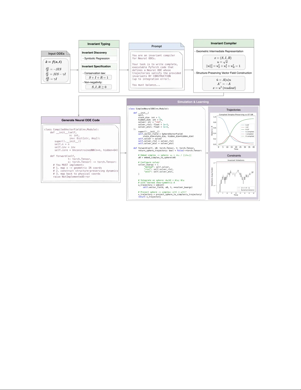
An In v arian t Compiler for Neural ODEs in AI-Accelerated Scien tiﬁc Sim ulation F angzhou Y u 1 , Yiqi Su 1 , Ray Lee 1 , Shenfeng Cheng 1 , and Naren Ramakrishnan 1 1 Virginia T ec h, V A, USA { yfangz7, yiqisu, ray.lee, chengsf, naren } @vt.edu Abstract Neural ODEs are increasingly used as con tinuous-time mo dels for scien tiﬁc and sensor data, but unconstrained neural ODEs can drift and violate domain inv ariants (e.g., conserv ation la ws), yielding ph ysically implausible solutions. In turn, this can compound error in long-horizon prediction and surrogate sim ulation. Existing solutions typically aim to enforce in v ariance b y soft penalties or other forms of regularization, whic h can reduce ov erall error but do not guaran tee that tra jectories will not lea ve the constrain t manifold. W e in tro duce the in v arian t compiler, a framework that enforces inv ariants by construction: it treats inv ariants as ﬁrst- class types and uses an LLM-driven compilation workﬂo w to translate a generic neural ODE sp eciﬁcation in to a structure-preserving arc hitecture whose tra jectories remain on the admissible manifold in con tinuous time (and up to numerical integration error in practice). This compiler view cleanly separates what m ust b e preserved (scien tiﬁc structure) from what is learned from data (dynamics within that structure). It provides a systematic design pattern for inv arian t- resp ecting neural surrogates across scientiﬁc domains. Keyw ords: Neural ODEs, Ph ysics-informed machine learning, In v ariant learning, Con tin uous time dynamical systems 1 In tro duction Learning dynamical systems from data is a cornerstone of mo dern science and engineering, with applications ranging from disco v ering ph ysical la ws [ 1 ] to building digital twins for complex indus- trial pro cesses [ 2 ]. Neural Ordinary Diﬀerential Equations (NODEs) ha ve emerged as a p o werful, general-purp ose framew ork for this task, parameterizing the v ector ﬁeld of a system’s dynamics with a neural net work [ 3 ]. Ho w ever, a fundamen tal c hallenge remains: standard data-driv en mo d- els are often “ph ysics-agnostic.” When deploy ed for long-horizon prediction, their tra jectories can drift, violating fundamen tal ph ysical principles suc h as conserv ation of energy , mass, or momen tum, leading to physically nonsensical and unreliable predictions [ 4 , 5 ]. Signiﬁcan t research has fo cused on embedding ph ysical priors into neural net work mo dels to mitigate these issues. These eﬀorts can b e broadly categorized into t w o paradigms. The ﬁrst approac h enforces in v arian ts through soft p enalties in the loss function, encouraging the mo del to resp ect a kno wn conserv ed quan tity [ 6 , 7 , 8 ]. While simple to implemen t, this provides no formal guaran tees; the learned dynamics can and do drift from the constraint manifold o ver time. 1 Figure 1: Inv arian t Compiler Pip eline for Neural ODEs. Epidemiological SIR dynamics are used as a representativ e example. The second paradigm seeks to enforce constraints exactly through architectural or algorithmic [ 9 , 10 ]. This includes pro jection-based metho ds that correct states onto v alid manifolds [ 11 , 12 , 13 , 14 ], energy-preserving architectures derived from Hamiltonian or Lagrangian mechanics [ 4 , 15 , 5 , 16 , 17 , 18 ], and netw orks enforcing stoichiometric or symmetry constrain ts [ 19 , 20 , 21 , 22 , 23 ]. While eﬀectiv e for their targeted inv ariants, these metho ds exist as a fragmented collection of point solutions, each requiring b esp ok e design for eac h new t yp e of constrain t. There lacks a unifying p erspective that treats ph ysical in v arian ts not as sp ecial cases, but as a fundamen tal aspect of the mo del’s t yp e signature. This fragmentation requires researchers to in ven t a new architecture for eac h new type of constrain t, hindering the rapid application of structured mo dels to new scien tiﬁc domains. In this work, w e prop ose an Inv arian t Compiler framew ork to bridge this gap via an LLM- driv en compilation workﬂo w. W e argue that inv ariants should b e treated as ﬁrst-class types that can b e systematically compiled into the structure of a Neural ODE. Our framework separates what m ust b e preserved (the structure, sp eciﬁed b y the in v arian t’s t yp e) from what must b e learned (the dynamics within that structure). The compiler takes a generic NODE v ector ﬁeld and systemati- cally rewrites it into an architecture whose tra jectories are guaranteed to remain on the admissible manifold in con tinuous time. W e demonstrate the unifying p o w er of this view by showing how a broad class of existing and nov el structure-preserving arc hitectures, e.g., from Hamiltonian me- c hanics to stoichiometric constraints, arise as instances of this compiler pip eline. 2 Our k ey con tributions are: (i) the in v ariant compiler design, (ii ) a cataloging of in v arian ts across m ultiple domains of physics, science, and engineering, and (iii) empirical results demonstrating constrain t satisfaction, forecasting and extrap olation accuracy , and ﬁdelity to underlying ph ysical structure and exp ected qualitative dynamics. 2 In v arian t Compiler Design W e treat inv ariants as ﬁrst-class types. A k ey design principle of the compiler is to separate what m ust b e preserved from what must b e learned. Once an inv ariant t yp e is sp eciﬁed, either from domain kno wledge or discov ered from data, the compiler deterministically pro duces a structure- preserving vector ﬁeld whose tra jectories remain on the v alid state manifold for all time. As sho wn in Fig. 1 , the compilation w orkﬂow consists of the follo wing stages. Stage 1: Input ODEs. The pip eline b egins with an input dynamical system speciﬁcation, e.g., ˙ x = f ( x, t ), provided in symbolic form or as executable co de. This reference ODE deﬁnes the in tended dynamics but is not required to satisfy inv ariants exactly [ 24 , 25 ]. It serves as the seman tic target that the compiled mo del aims to preserv e while enforcing additional structure. Stage 2: In v arian t T yping (Discov ery or Sp eciﬁcation). Inv ariants are obtained through t wo complemen tary mec hanisms. (i) Invariant disc overy : when inv ariants are unknown, data- driv en metho ds such as sym b olic regression are used to prop ose candidate conserved quantities or constrain ts [ 26 , 27 , 28 , 29 ]. (ii) Invariant sp e ciﬁc ation : when in v ariants are kno wn, users explicitly pro vide constrain ts suc h as conserv ation laws, non-negativity , ordering constrain ts, energetic struc- ture, or stoic hiometric balances [ 4 , 16 , 30 , 31 , 32 ]. T ogether, these inv ariants deﬁne the admissible state manifold on whic h the dynamics m ust ev olv e. Stage 3: Prompt (Program Speciﬁcation). The input ODEs and the typed in v arian ts are assem bled in to a structured prompt that serv es as the compiler’s program speciﬁcation. The prompt enco des the base dynamics, the in v arian ts to b e preserved, and hard compilation constraints (e.g., in v arian ts must hold by construction, without p enalties or p ost-hoc pro jection). This step makes the in terface b et w een user in tent and the compiler explicit, while the downstream compilation remains deterministic and t yp e-driv en [ 33 ]. T able A6 summarizes the prompt v arian ts supp orted b y the in v arian t compiler and their corresp onding inv ariant types and structure-preserving rewrite rules. Stage 4: In v arian t Compiler. The inv ariant compiler interprets the prompt and performs t wo tigh tly coupled steps: (i) Ge ometric Interme diate R epr esentation (IR) : each in v arian t type is mapp ed to a geometric or algebraic represen tation in whic h the constraint becomes structural (e.g., simplices to spheres, conserv ation la ws to null spaces, PSD constrain ts to Cholesky manifolds, en- ergy conserv ation to symplectic or P oisson manifolds). (ii) Structur e-Pr eserving V e ctor Field Con- struction : the vector ﬁeld is rewritten in to a form that is tangen t to the admissible manifold, using in v arian t-sp eciﬁc constructions such as skew-symmetric generators, null-space parameterizations, factorized dynamics, Hamiltonian/Poisson formulations, or tangent-cone pro jections. This stage constitutes the core compilation step and guaran tees exact in v ariance in contin uous time. 3 Stage 5: Generate Neural ODE Co de. The compiler emits executable Neural ODE co de (e.g., a PyT orc h nn.Module implementing forward(t,x) ), in which the inv ariant-preserving structure is ﬁxed and only unconstrained submo dules (e.g., neural netw orks pro ducing interaction terms, matrices, or reaction rates) are learnable. The generated co de also includes in v arian t diagnostics for v eriﬁcation. Stage 6: Sim ulation & Learning. Finally , the generated Neural ODE is executed in a standard run-time loop using an ODE solver and, when applicable, trained on data. Because in v ariants are enforced b y construction in the compiled v ector ﬁeld, sim ulation and learning proceed without p enalties, normalization, or p ost-ho c pro jection, up to numerical integration error. 3 Catalog of In v arian t T yp es T able 1 summarizes the inv ariant types supported b y the compiler, along with their geometric represen tations, enforcement mec hanisms, and represen tative applications. W e describe each t yp e b elo w; full mathematical deriv ations and formal veriﬁcation pro ofs app ear in App endices A – I . 3.1 Simplex Preserv ation via Sk ew-Symmetric Dynamics Systems whose states represen t prop ortions or frequencies—suc h as compartmental epidemiological mo dels (SIR, SEIR) [ 34 , 35 , 36 ], market shares [ 37 ], or allele frequencies [ 38 ]—m ust remain on the probabilit y simplex [ 39 ] ∆ n − 1 = { x ∈ R n : P i x i = 1 , x i ≥ 0 } . W e enforce simplex inv ariance via a three-step construction inspired by the analogy b et ween probabilit y simplices and quantum state spaces [ 40 , 41 ]. First, we em b ed the simplex into the unit sphere S n − 1 via the square-root map u i = √ x i , so that ∥ u ∥ 2 2 = P i x i = 1. Second, we ev olv e u ( t ) on the sphere using skew-symmetric dynamics: du dt = A ( u ) u, A ( u ) = 1 2 ( f θ ( u ) − f θ ( u ) ⊤ ) , (1) where f θ is a neural netw ork. Since A ⊤ = − A , we ha ve u ⊤ Au = 0, whic h preserves ∥ u ∥ 2 = 1. Third, we recov er simplex co ordinates via squaring: x i ( t ) = u i ( t ) 2 . Non-negativity is automatic ( u 2 i ≥ 0), and the sum constrain t follo ws from norm preserv ation ( P i u 2 i = 1). See App endix A for the full deriv ation. 3.2 Cone In v arian ts via T angen t-Space Pro jection Man y ph ysical systems ev olv e within conic regions of state space—sets closed under p ositiv e scaling. Tw o cones arise frequentl y . Loren tz Cone. Giv en a system dz dt = f ( z ) , (2) the constraint z ∈ L n +1 app ears in relativistic causal structure [ 42 ] and robust optimization [ 43 ], where the Lorentz cone L n +1 is deﬁned by L n +1 = { ( t, x ) ∈ R × R n : t ≥ ∥ x ∥ 2 } . (3) 4 T able 1: Catalog of inv ariant types supp orted by the In v arian t Compiler. Eac h row shows one in v arian t type with its c onstrain t, the geometric or algebraic mec hanism used to enforce it, and represen tative application domains. F ull deriv ations and pro ofs app ear in the referenced app endix. In v arian t T yp e Constrain t Geometric IR Enforcemen t Mech- anism Applications Key Refs. App. Simplex / Norm P i x i = 1, x i ≥ 0 Unit sphere S n − 1 via √ · map Sk ew-sym. dynamics: ˙ u = A ( u ) u , A ⊤ = − A ; x i = u 2 i Epidemiology , mark et share, p op. genetics [ 40 , 41 ] A Loren tz Cone t ≥ ∥ x ∥ 2 Loren tz cone L n +1 T angent-cone pro j.: ˙ z = π T K ( z ) ( ˆ f θ ( z )) Relativit y , ro- bust opt., signal pro c. [ 45 , 42 , 49 ] B PSD Cone P ⪰ 0 Cholesky manifold Cholesky param.: P = LL ⊤ , evolv e L Co v ariance dy- namics, Kalman ﬁltering [ 47 , 48 ] C Cen ter of Mass P i m i r i = 0 , P i m i v i = 0 Null space of mass- w eighted sum Mean subtraction: ˙ r i = v i − ¯ v , ˙ v i = a i − ¯ a N -b ody , molecu- lar dynamics [ 50 , 51 ] D Stoic hiometric M c ( t ) = const Null space of molecular ma- trix M Null-space pro j.: ˙ c = B · r θ ( c, t ), M B = 0 Chemical kinet- ics, metabolic net works [ 21 , 20 ] E Hamiltonian dH dt = 0, Jacobi iden tity Symplectic / P oisson mani- fold Laten t canonical co- ords via INN: ˙ z = J 0 ∇ z K ( z ) P endulum, Lotk a-V olterra, rigid b ody [ 52 ] F P ort-Hamil. dH dt ≤ 0 P oisson + PSD dissipa- tion ˙ z = [ J 0 − R ( z )] ∇ z K ( z ), R = LL ⊤ ⪰ 0 Damp ed oscilla- tors, circuits [ 17 ] G GENERIC dH dt = 0, dS dt ≥ 0 Poisson + pro j. dissipa- tion Casimir-dep. entrop y + pro j. M z Thermomec h., p olymer relax- ation [ 18 , 53 ] H First In te- gral V ( u ( t )) = const (learned) Learned con- strain t mani- fold T angent-space pro j.: ( I − ∇ V ⊤ ( ∇ V ∇ V ⊤ ) + ∇ V ) ˆ f ( u ) Unkno wn con- serv ation la ws [ 54 , 11 ] I F orward in v ariance is enforced by pro jecting the learned neural vector ﬁeld ˆ f θ on to the tangen t cone at each p oin t [ 44 ]: dz dt = f θ ( z ) : = π T K ( z ) ( ˆ f θ ( z )) , z (0) ∈ K, (4) where K : = L n +1 and π T K ( z ) denotes orthogonal pro jection on to the tangent cone T K ( z ). The viabilit y condition f θ ( z ) ∈ T K ( z ) guarantees that tra jectories starting in K remain in K [ 45 ]. The pro jection has closed-form expressions for interior, b oundary , and ap ex cases (App endix B ). PSD Cone. The constrain t P ⪰ 0 arises in cov ariance dynamics and ﬁltering [ 46 ]. Rather than pro jecting onto S n + (requiring eigen v alue decomp osition), w e employ a Cholesky parameterization [ 47 , 48 ]: evolv e a lo w er-triangular factor L ( t ) via dL dt = g θ ( L ) and reco v er P ( t ) = L ( t ) L ( t ) ⊤ . Sym- metry and positive semideﬁniteness hold automatically since v ⊤ LL ⊤ v = ∥ L ⊤ v ∥ 2 ≥ 0 (App endix C ). 5 3.3 Cen ter of Mass F rame Constrain ts F or isolated n -b ody systems, conserv ation of total momen tum implies in v ariance of the center of mass frame: P i m i r i = 0 and P i m i v i = 0 [ 50 , 51 , 55 ]. These constrain ts need not be hard compiled into the neural ODE arc hitecture; we include them as a useful inductiv e bias that is often encountered in real systems. Given predicted accelerations a i = f θ ( r , v ) i , w e enforce these constrain ts b y subtracting the mass-w eighted mean: d r i dt = v i − ¯ v , d v i dt = a i − ¯ a , (5) where ¯ v = P k m k v k P k m k and ¯ a = P k m k a k P k m k . This pro jects out an y net translation or force, ensuring the neural net w ork’s output aﬀects only relativ e (internal) dynamics (App endix D ). 3.4 Stoic hiometric Constrain ts via Null-Space Pro jection Chemical and biological systems ob ey elemen tal conserv ation: atoms are rearranged but never created or destroy ed [ 56 ]. F or sp ecies concentrations c ( t ), these laws tak e the form M c ( t ) = M c (0), where the molecular matrix M enco des elemen t-to-sp ecies coun ts. W e parameterize dynamics via the n ull-space basis B of M [ 21 , 20 ]: dc dt = B r θ ( c, t ) , (6) where r θ : R n × R → R k is a neural netw ork and k = dim(Null( M )). Since M B = 0 b y construction, w e hav e M ˙ c = 0, guaranteeing exact elemen tal conserv ation regardless of the netw ork output (App endix E ). 3.5 Hamiltonian / P oisson Structure Man y ph ysical systems conserve energy exactly when dissipation is absent [ 57 ]. The dynamics tak e the form ˙ u = J ( u ) ∇ u H ( u ), where H is the Hamiltonian [ 58 , 4 ] and the skew-symmetric matrix J ( u ) deﬁnes a Poisson structure satisfying the Jacobi iden tit y [ 59 ]. Rather than learning a state-dep enden t J ( u ) sub ject to the nonlinear Jacobi iden tity constraint, follo wing Jin et al. [ 52 ], we adopt a latent-space approac h[ 60 ]. An inv ertible neural netw ork g θ : u ↔ z = ( q , p, c ) maps physical co ordinates to latent canonical co ordinates, where the dynamics b ecome: dz dt = J 0 ∇ z K ( z ) , J 0 =   0 I d 0 − I d 0 0 0 0 0   , (7) with K ( z ) := H ( g − 1 θ ( z )). Energy conserv ation follows from sk ew-symmetry (( ∇ K ) ⊤ J 0 ( ∇ K ) = 0), and the Jacobi identit y holds automatically for the constant canonical matrix J 0 . Casimir co ordinates c are frozen b y the zero blo c k, enco ding additional conserved quanti ties. The physical P oisson matrix J ( u ) is induced via the co ordinate transformation law, inheriting the Jacobi iden tity from J 0 (App endix F ). 3.6 P ort-Hamiltonian (Dissipativ e) Structure Systems with friction, damping, or irreversible losses satisfy dH dt ≤ 0 [ 61 ]. F ollo wing Cheng et al. [ 17 ], w e augmen t the canonical latent-space dynamics with a p ositiv e semi-deﬁnite dissipation matrix R z : dz dt = [ J 0 − R z ( z )] ∇ z K ( z ) , (8) 6 where R z ( z ) = L θ ( z ) L θ ( z ) ⊤ ⪰ 0 and the mapping L θ ( z ) is parameterized by a neural net work. The energy rate b ecomes dK dt = − ( ∇ z K ( z )) ⊤ R z ( z )( ∇ z K ( z )) ≤ 0, guaran teeing passiv e stability by construction (Appendix G ). 3.7 GENERIC / Thermo dynamic Structure Thermo dynamic systems exhibit b oth reversible (energy-conserving) and irreversible (entrop y- pro ducing) dynamics, gov erned b y the GENERIC formalism [ 62 ]: ˙ u = J ∇ H + M ∇ S , sub ject to degeneracy conditions J ∇ S = 0 and M ∇ H = 0. Here, S denotes the entrop y functional and M ⪰ 0 is a positive semi-deﬁnite friction matrix go v erning irreversible dissipation. W e enforce these in latent space via tw o arc hitectural choices [ 18 , 53 ]: 1. Casimir-dep enden t entrop y : S ( z ) = ˜ S ( c ), so ∇ z S = (0 , 0 , ∇ c ˜ S ) ⊤ lies in the null space of J 0 . 2. Pro jected dissipation : M z = P K c M z P K , where P K = I − ∇ K ( ∇ K ) ⊤ ∥∇ K ∥ 2 + ε pro jects onto constant- energy surfaces. T ogether, these guarantee energy conserv ation ( dH dt = 0), non-negativ e en tropy pro duction ( dS dt ≥ 0), and both degeneracy conditions—all b y construction (Appendix H ). 3.8 First In tegral Preserv ation via Manifold Pro jection When conserv ed quantities V ( u ) ∈ R m are unkno wn, following Matsubara and Y aguchi [ 54 ], w e learn them as neural net works V i ( u ; ϕ i ) (1 ≤ i ≤ m ) and, follo wing White et al. [ 11 ], pro ject an unconstrained base v ector ﬁeld ˆ f ( u ) on to the tangent space of the learned constraint manifold [ 49 ]: du dt = ( I − P ( u )) ˆ f ( u ) , P = ∇ V ⊤ ( ∇ V ∇ V ⊤ ) + ∇ V , (9) where ( · ) + is the Mo ore–P enrose pseudo-in v erse. The pseudo-in v erse gracefully handles redundant constrain ts: if the net work disco vers linearly dep enden t conserved quan tities, the pro jection remains w ell-deﬁned. Since ( I − P ) pro jects on to n ull( ∇ V ), w e ha ve ∇ V ⊤ i ( I − P ) = 0, ensuring all ﬁrst in tegrals are exactly preserv ed (App endix I ). 4 Exp erimen ts 4.1 Setup W e ev aluate the In v arian t Compiler across dynamical systems spanning geometric, algebraic, ener- getic, and thermo dynamic inv ariants (T able 2 ); full equations and parameters are in App endix J . 4.1.1 Researc h Questions W e ev aluate the In v arian t Compiler framew ork through exp erimen ts designed to address the fol- lo wing research questions, each tested on a primary system (b old) and, where applicable, a supple- men tary system whose results appear in Appendix K : Q1 Constrain t satisfaction. Do compiled arc hitectures enforce algebraic constrain ts to numerical precision? Primary: NOx reaction net w ork . Supplemen tary: SIR mo del, c hemical reaction net work. Q2 Prediction accuracy . Do es enco ding constrain ts impro ve or degrade prediction accuracy? Primary: coupled radial-angular dynamics . Supplementary: Lorentz cone spiral. 7 T able 2: Catalog of dynamical systems used in the exp erimen ts. Eac h system is designated with its dimensionalit y , the inv ariant type, and the compiled arc hitecture used to enforce the in v arian t. System Dim. In v ariant type Arc hitecture Key challenge SIR epidemiological mo del 3 Simplex ( S + I + R =1) Sk ew-symmetric P opulation conserv ation NOx reaction netw ork 5 Stoichiometric ( S ˙ c = 0 ) Null-space Nonlinear kinetics, pro duct inhibition Chemical reaction netw ork 6 Stoichiometric ( S ˙ c = 0 ) Null-space Element conservation (C, H, O) Lorentz cone spiral 3 Cone ( t ≥ ∥ x ∥ 2 ) Pro jection Boundary dynamics Coupled radial-angular dynamics 3 Cone ( t ≥ ∥ x ∥ 2 ) Pro jection Nonlinear radial-angular coupling Replicator-mutator ( N =5) 5 Simplex ( P x i =1) Skew-symmetric Diverse dynamical regimes Lotk a-V olterra predator-prey 2 Hamiltonian (Poisson) Poisson INN Non-canonical brack et Damped harmonic oscillator 2 Port-Hamiltonian ( ˙ E ≤ 0) PH-INN Energy dissipation Thermomechanical system 3 GENERIC ( ˙ E =0, ˙ S ≥ 0) GENERIC INN Coupled conserv ation + pro duction Extended p endulum 3 Poisson (Casimir + Hamiltonian) Poisson INN Multiple simultaneous inv ariants Two-body gravitational 8 Mixed (known + learned) FINDE Heterogeneous inv arian t comp osition Q3 Long-horizon extrap olation. Do compiled architectures maintain bounded errors at 2 × – 10 × the training horizon? Primary: thermomec hanical system . Supplemen tary: damp ed harmonic oscillator. Q4 Conserv ation la w ﬁdelit y . Do learned inv ariants trac k theoretically predicted quan tities? Primary: Lotk a-V olterra system . Q5 Qualitativ e b eha viour. Do compiled architectures repro duce the correct dynamical regime? Primary: Replicator-mutator system . Q6 Scalabilit y . Do compiled constrain ts remain eﬀective with m ultiple simultaneous in v arian ts and higher structural complexity? Primary: extended p endulum . Q7 Comp osabilit y . Can heterogeneous in v arian t t yp es—some known analytically , others learned— b e comp osed within a single architecture? Primary: t w o-b o dy gravitational system . 4.1.2 T raining, Arc hitecture, Baselines, and Metrics In tegration and T raining. All mo dels emplo y fourth-order Runge-Kutta (RK4) in tegration during both training and inference. W e use m ulti-step rollouts with exp onen tially deca ying w eights: L = 1 n steps n steps X k =1 1 k ∥ ˆ u t + k − u t + k ∥ 2 , (10) with n steps = 4, emphasising accurate short-term prediction while p enalising long-horizon drift. Mo dels are optimised using AdamW with learning rate 10 − 3 , w eight decay 10 − 5 , and cosine an- nealing o ver 300–1000 epo c hs depending on the task. Gradient norms are clipp ed to 1.0 for stabilit y . Net w ork Arc hitecture. All metho ds share iden tical netw ork capacity where applicable. F or direct constrain t enforcemen t exp erimen ts, we emplo y 3-la y er MLPs with 64 hidden units and SiLU (or Softplus for chemical systems) activ ations. F or structure-learning exp eriments, we additionally use: In v ertible Neural Netw ork (INN): 8 coupling blo c ks using the AllInOneBlo c k architecture from F rEIA [ 63 ], with soft p erm utations b et w een blo c ks. Eac h coupling block uses a 3-la yer MLP subnet with hidden dimension 64 and SiLU activ ations. Dissipation netw orks: 3-lay er MLPs outputting Cholesky factors, initialised with small w eigh ts ( σ = 0 . 01) for stability . 8 LLM Implemen tation. The in v arian t compiler uses a large language mo del (LLM) as a program syn thesis and rewrite engine, rather than as a predictive mo del. Given the prompt sp eciﬁcation (Listing 1 ), the LLM generates executable PyT orc h co de that implemen ts the required geometric in termediate representation and structure-preserving v ector ﬁeld. All compilation logic is driv en by the prompt and deterministic p ost-processing; the LLM is not trained or ﬁne-tuned on the target dynamical systems. Unless otherwise stated, we use a standard GPT-class mo del with temp erature set to zero to ensure deterministic code generation. Baselines. All exp erimen ts compare against an Unconstrained (Neural ODE) baseline: a v anilla Neural ODE that directly parameterises the vector ﬁeld ˙ x = f θ ( x ) without an y structural constrain ts. The t w o exp erimen tal sections employ diﬀeren t soft-constrain t baselines suited to their respective settings. F or constrain t satisfaction exp erimen ts (Sections 4.2 – 4.3 ), w e additionally compare against a P enalty baseline trained with an additional p enalt y term λ · L constraint ( λ = 10). F or structure-learning exp erimen ts (Sections 4.4 – 4.5 ), we instead compare against a PINNs-style baseline that augmen ts the Neural ODE loss with physics-informed p enalt y terms derived from the known analytical form of the system’s in v arian ts. Metrics. W e ev aluate mo dels using tra jectory MSE (rep orted separately for training window, extrap olation window, and total) and constraint-speciﬁc measures. F or systems with explicit con- strain ts, we rep ort mean violation; for systems with conserved quantities, we measure deviation from theoretical v alues: Deviation = 1 T Z T 0 | Q ( t ) − Q theory ( t ) | dt. (11) T o make relative p erformance transparen t, we additionally rep ort impr ovement factors (IF): the ratio of the best baseline metric to the compiled-architecture metric. 4.2 Q1: Constrain t Satisfaction W e ev aluate whether compiled architectures can enforce hard algebraic c onstrain ts to numerical precision, using the NOx reaction netw ork—a system with strongly nonlinear kinetics including pro duct inhibition, substrate inhibition, and fractional-p ow er terms. W e train on 1000 tra jectories ( T end =10, 200 p oin ts p er tra jectory) and ev aluate on 200 held-out initial conditions. Results for the supplementary systems (SIR mo del, six-sp ecies c hemical netw ork) app ear in App endix K , T ables A1 – A2 . The stoichiometric matrix S ∈ R 2 × 5 enco des elemen t-to-sp ecies relationships for nitrogen and o xygen. F ollo wing Section 3.4 , w e parameterise dynamics via the n ull-space basis, ensuring S · ˙ c = 0 b y construction. T able 3: NOx reaction netw ork ( Q1 : constraint satisfaction). Mean ± std o ver 200 test tra jectories. IF = improv emen t factor of our method o v er the best baseline. Metric Unconst. P enalt y Ours IF MSE (T rain) 5 . 86e-7 ± 6 . 10e-7 1 . 02e-2 ± 1 . 02e-2 1 . 80 e- 7 ± 1 . 48e-7 3 . 3 × MSE (Extrap) 1 . 23e-6 ± 1 . 68e-6 1 . 22e-2 ± 1 . 10e-2 9 . 18 e- 8 ± 8 . 39e-8 13 × MSE (T otal) 9 . 09e-7 ± 1 . 04e-6 1 . 12e-2 ± 1 . 06e-2 1 . 36 e- 7 ± 9 . 19e-8 6 . 7 × Elem. Dev. 6 . 80e-3 ± 4 . 15e-3 1 . 10e-4 ± 7 . 42e-5 1 . 06 e- 6 ± 8 . 26e-7 104 × 9 T able 3 demonstrates that the null-space arc hitecture reduces element conserv ation violations b y ov er t wo orders of magnitude (104 × ) compared to the best baseline (p enalt y), and b y nearly four orders of magnitude compared to the unconstrained mo del. Element deviations remain at ∼ 10 − 6 (near n umerical precision), whereas soft penalties reduce violations only to ∼ 10 − 4 while substan tially degrading MSE. Consistent results are observed for the simpler SIR and chemical systems (App endix K ), where compiled architectures ac hiev e 6 and 4 orders of magnitude violation reduction, respectively . 0 8 16 0.0 0.2 0.4 (a) 0 8 16 0.0 0.2 0.4 (b) 0 8 16 0.00 0.15 0.30 (c) T ruth Unconstr . P enalty Ours Figure 2: NOx reaction net work ( Q1 ). T ra jectory comparison showing sp ecies concen trations ov er time under three diﬀerent initial conditions: (a), (b), and (c). Each initial condition leads to distinct transient dynamics and con v erges to diﬀeren t equilibrium v alues. The v ertical dashed line marks the end of the training windo w. 4.3 Q2: Prediction Accuracy W e ev aluate whether compiled constrain ts impro ve or degrade prediction accuracy , using coupled radial-angular dynamics on the Lorentz cone—a system with nonlinear coupling b et ween radial gro wth and angular velocity . W e train on 1000 tra jectories ( T end =10, 500 p oin ts) and ev aluate on 200 held-out tra jectories to T end =16 (1 . 6 × extrap olation). Results for the supplementary system (simple Loren tz cone spiral) appear in Appendix K , T able A3 . The pro jection-based architecture guaran tees that all predicted tra jectories remain within the cone L 3 . T able 4: Coupled radial-angular dynamics on the Lorentz cone ( Q2 : prediction accuracy). Mean ± std ov er 200 test tra jectories. Metric Unconst. P enalty Ours IF MSE (T rain) 3 . 04e-4 ± 2 . 46e-3 2 . 45e-1 ± 8 . 31e-1 1 . 02 e- 4 ± 4 . 81e-4 3 . 0 × MSE (Extrap) 4 . 90e-4 ± 4 . 03e-3 4 . 43e-1 ± 1 . 40e+0 1 . 55 e- 4 ± 7 . 55e-4 3 . 2 × MSE (T otal) 3 . 74e-4 ± 3 . 05e-3 3 . 20e-1 ± 1 . 05e+0 1 . 22 e- 4 ± 5 . 84e-4 3 . 1 × Viol. (Mean) 4 . 13e-4 ± 4 . 37e-4 1 . 07 e- 11 ± 3 . 30e-11 3 . 75e-11 ± 1 . 34e-10 — T able 4 reveals a key ﬁnding: the Loren tz PDS arc hitecture ac hiev es 3 × lo wer tra jectory MSE than the unconstrained baseline while main taining cone violations near n umerical precision ( ∼ 10 − 8 ). Unlik e the simple spiral (App endix K ), where unconstrained mo dels could gain slight MSE adv an- 10 tages by “shortcutting” through forbidden cone interiors, the coupled radial-angular dynamics de- mand accurate modelling of the in terpla y betw een radial gro wth and angular v elo cit y—a task where geometric consistency pro vides a genuine inductive bias. The p enalt y baseline, while achieving low violations, catastrophically degrades prediction accuracy (MSE > 10 − 1 ), demonstrating once more that soft-constrain t regularisation fundamen tally conﬂicts with the data-ﬁtting ob jectiv e. 4 0 4 4 0 4 0 2 4 (a) 3 0 3 3 0 3 (b) 0 6 12 4 0 4 (c) T ruth Unconstr . P enalty Ours Figure 3: Coupled radial-angular dynamics on the Loren tz cone ( Q2 ). (a) T ra jectories in 3D cone space. (b) Pro jection onto the ( x 1 , x 2 ) plane. (c) Time ev olution of the temp oral comp onen t t , radial norm | x | , and spatial co ordinates x 1 , x 2 , with the vertical dashed line marking the training horizon. 4.4 Q3: Long-Horizon Extrap olation W e ev aluate the ability of compiled architectures to main tain accuracy o ver extended time hori- zons, using the thermomec hanical system—a damp ed oscillator coupled to a heat bath where total energy is conserv ed while entrop y increases monotonically . T raining uses a single tra jectory of 1000 p oin ts o ver t ∈ [0 , 30], with ev aluation at 2 × , 5 × , and 10 × the training horizon. Results for the supplemen tary system (damp ed harmonic oscillator) app ear in Appendix K , T able A4 . T able 5 reveals a striking pattern: at 10 × extrap olation, the GENERIC INN maintains MSE b elo w 10 − 6 while the Neural ODE degrades to 2 . 1 × 10 − 4 —o ver 200 × w orse. Even the PINNs- st yle baseline, despite access to the true analytical inv ariants, degrades to 1 . 0 × 10 − 5 , more than 10 × w orse than the compiled architecture. The improv emen t factors gro w with the extrap olation horizon, underscoring that hard structural enforcemen t provides compounding b eneﬁts ov er time: soft constrain ts “leak” gradually , whereas c ompiled constraints remain exact. Energy deviation at 10 × reac hes 2 . 3 × 10 − 2 for the Neural ODE but only 1 . 3 × 10 − 3 for the GENERIC INN—an 18 × impro vemen t. 4.5 Q4: Conserv ation La w Fidelity W e ev aluate whether compiled architectures faithfully maintain the underlying conserv ation struc- ture, using the Lotk a-V olterra predator-prey system. T raining data spans t ∈ [0 , 30] (single tra jec- tory), with ev aluation at 2 × , 5 × , and 10 × extrap olation. T able 6 shows that the Poisson INN achiev es the tightest energy deviation at b oth 5 × and 10 × extrap olation, despite never having ac c ess to the analytic al Hamiltonian . The learned Hamiltonian deviation remains b ounded ( < 4 . 2 × 10 − 4 ) ev en at 10 × extrap olation, whereas the Neural ODE’s deviation gro ws to 3 . 4 × 10 − 3 —an 8 . 3 × gap. The PINNs-st yle baseline, whic h directly penalises the kno wn conserv ed quan tity , ac hiev es comp etitiv e short-horizon ﬁdelit y but falls b ehind the P oisson 11 T able 5: Thermomechanical system ( Q3 : long-horizon extrapolation). A single training tra jectory is extrapolated to 2 × , 5 × , and 10 × the training horizon. IF at 10 × relativ e to best baseline. Metric Model × 2 × 5 × 10 IF ( × 10 ) MSE (T rain) Unconst. 2.91e-06 2.91e-06 2.91e-06 PINNs 2.56e-06 2.56e-06 2.56e-06 Ours 1.16e-06 1.16e-06 1.16e-06 2 . 2 × MSE (Extrap) Unconst. 2.41e-05 1.40e-04 2.33e-04 PINNs 2.16e-06 6.75e-06 1.12e-05 Ours 7.21e-07 8.47e-07 9.77e-07 11 × MSE (T otal) Unconst. 1.35e-05 1.13e-04 2.10e-04 PINNs 2.36e-06 5.91e-06 1.03e-05 Ours 9.40e-07 9.10e-07 9.95e-07 10 × Energy Dev. Unconst. 4.80e-03 1.56e-02 2.29e-02 PINNs 8.50e-04 3.26e-03 4.94e-03 Ours 9.24e-04 1.11e-03 1.27e-03 3 . 9 × En tropy Dev. Unconst. 2.18e-03 6.97e-03 1.02e-02 PINNs 4.02e-04 1.46e-03 2.20e-03 Ours 3.63e-04 4.75e-04 5.53e-04 4 . 0 × 0.0 1.5 1 0 1 1.0 1.5 2.0 (a) 1.5 0.0 1.5 0.0 1.5 1.8 2.1 2.4 (b) T ruth Unconstr . PINNs Ours Figure 4: 3D phase-space p ortraits. (a) Thermomec hanical system ( Q3 ) (b) Extended pendulum ( Q6 ) Green dots indicate initial conditions. 12 T able 6: Lotk a-V olterra system ( Q4 : conserv ation la w ﬁdelity). IF at 10 × relativ e to b est baseline. Metric Model × 2 × 5 × 10 IF ( × 10 ) MSE (T rain) Unconst. 4.39e-06 4.39e-06 4.39e-06 PINNs 7.54e-06 7.54e-06 7.54e-06 Ours 7.61e-07 7.61e-07 7.61e-07 5 . 8 × MSE (Extrap) Unconst. 7.38e-05 1.08e-03 1.15e-02 PINNs 6.03e-05 1.66e-04 3.47e-04 Ours 2.25e-06 1.11e-05 4.76e-05 7 . 3 × MSE (T otal) Unconst. 3.91e-05 8.63e-04 1.04e-02 PINNs 3.39e-05 1.34e-04 3.13e-04 Ours 1.51e-06 9.00e-06 4.29e-05 7 . 3 × Energy Dev. Unconst. 1.18e-03 2.14e-03 3.44e-03 PINNs 2.14e-04 4.23e-04 6.15e-04 Ours 3.80e-04 3.99e-04 4.14e-04 1 . 5 × INN at 5 × and 10 × , illustrating that soft p enalties inevitably drift. The Poisson INN sim ultane- ously achiev es 7 × low er tra jectory MSE at 10 × extrap olation, conﬁrming that structure ﬁdelit y and prediction accuracy are mutually reinforcing. 4.6 Q5: Qualitativ e Beha viour W e ev aluate whether compiled arc hitectures repro duce the correct qualitative dynamics—oscillatory , con vergen t, or transient behaviour depending on initial conditions—using the Replicator-Mutator system ( N =5 sp ecies). W e train on 1000 tra jectories sampled from a Dirichlet distribution and ev aluate on 200 held-out tra jectories o ver t ∈ [0 , 20]. T able 7: Replicator-Mutator system, N =5 ( Q5 : qualitative b eha viour). Mean ± std o v er 200 test initial conditions. Metric Unconst. Penalt y Ours IF MSE (T rain) 8 . 31e-5 ± 1 . 83e-4 1 . 03e-2 ± 1 . 33e-2 1 . 38 e- 5 ± 3 . 62e-5 6 . 0 × MSE (Extrap) 7 . 46e-5 ± 1 . 60e-4 7 . 81e-3 ± 1 . 33e-2 1 . 19 e- 5 ± 2 . 75e-5 6 . 3 × MSE (T otal) 7 . 88e-5 ± 1 . 71e-4 9 . 07e-3 ± 1 . 18e-2 1 . 28 e- 5 ± 3 . 18e-5 6 . 2 × Viol. (Mean) 3 . 08e-4 ± 6 . 54e-5 3 . 11e-4 ± 1 . 75e-4 2 . 79 e- 5 ± 6 . 97e-6 11 × T able 7 shows that the skew-symmetric architecture ac hieves b oth 6 × low er tra jectory MSE and 11 × lo wer simplex violation than the b est baseline. This combination is essential for qualitativ e ﬁdelit y: maintaining simplex mem b ership ( P x i = 1, x i ≥ 0) ensures that predicted sp ecies fre- quencies remain biologically meaningful, while low er MSE ensures the correct dynamical regime is repro duced. The penalty metho d fails dramatically: comp eting with the data-ﬁtting loss degrades MSE b y nearly three orders of magnitude while ac hieving negligible violation improv emen t. 4.7 Q6: Scalabilit y W e test whether compiled constrain ts remain eﬀective as structural complexit y gro ws, using the extended pendulum—a system that requires sim ultaneous preserv ation of a Hamiltonian and a Casimir inv ariant in a state-dep enden t Poisson structure. T raining uses a single tra jectory o ver t ∈ [0 , 30]. F ull results app ear in T able A5 (App endix K.5 ). 13 0 15 30 0.00 0.25 0.50 (a) 0 15 30 0.00 0.25 0.50 (b) 0 15 30 0.0 0.2 0.4 (c) T ruth Unconstr . P enalty Ours Figure 5: Replicator-Mutator system ( Q5 ). T ra jectories for three held-out initial conditions ex- hibiting qualitativ ely diﬀeren t dynamics: (a) transien t oscillation, (b) monotone c on v ergence, and (c) sustained oscillations. The v ertical dashed line marks the training horizon. Enforcing tw o inv ariants sim ultaneously do es not degrade performance – in con trast, the Poisson INN ac hiev es 40 × lo wer extrap olation MSE than the Neural ODE and four orders of magnitude lo wer than the p enalt y baseline at 10 × extrap olation. Both Casimir and Hamiltonian deviations remain tightly b ounded, conﬁrming that compiled constraints scale gracefully when multiple in- v arian ts m ust b e enforced simultaneously . Figure 4 (b) shows the Poisson INN tracking the true tra jectory through 10 × extrap olation in the ( u, v , r ) co ordinate space. 4.8 Q7: Composability Finally , w e test whether inv ariants of heterogeneous t yp e—some analytically kno wn, others learned from data—can b e comp osed within a single compiled arc hitecture, using the equal-mass t wo-bo dy gra vitational problem with four simultaneous conserv ed quantities. W e train on 1000 tra jectories (500 steps p er tra jectory) and ev aluate on 200 held-out tra jectories o ver 4 × the training horizon. F ollowing Section 3.8 , w e enforce all four in v arian ts through manifold pro jection. The momen- tum constraints p x ( u ) = ˙ x 1 + ˙ x 2 and p y ( u ) = ˙ y 1 + ˙ y 2 are embedded as known analytical gradien ts, while t wo additional conserv ed quantities are learned: a Hamiltonian net work H ϕ ( u ) and a general ﬁrst-in tegral net work V ψ ( u ). T able 8: Tw o-bo dy gra vitational system ( Q7 : composability). Mean ± std o ver 200 test tra jecto- ries. IF relativ e to b est baseline. Metric Unconst. PINNs Ours IF MSE (T otal) 2.01e-05 ± 1.79e-05 6.75e-05 ± 9.91e-05 2.92e-06 ± 1.62e-06 6 . 9 × Energy Dev. 2.94e-04 ± 2.49e-04 4.84e-04 ± 3.04e-04 1.81e-04 ± 9.11e-05 1 . 6 × Momen tum Dev. 1.77e-04 ± 6.89e-05 5.18e-04 ± 2.51e-04 2.42e-07 ± 1.16e-07 731 × Ang-Mom Dev. 4.86e-04 ± 4.61e-04 7.07e-04 ± 4.95e-04 2.75e-04 ± 1.78e-04 1 . 8 × T able 8 demonstrates that heterogeneous in v arian t t yp es compose eﬀectively . The analytically em b edded momen tum constrain ts yield the most dramatic result: momen tum deviation drops to ∼ 10 − 7 , a 731 × improv emen t ov er the b est baseline. Crucially , embedding the known constrain ts do es not imp ede learning of unkno wn ones—energy and angular momen tum deviations are also the lo west among all metho ds, and total tra jectory MSE improv es b y 6 . 9 × ov er the unconstrained 14 Neural ODE. The PINNs-style baseline, despite p enalising all four kno wn in v arian ts, actually p er- forms worse than the unconstrained mo del on MSE and sev eral deviation metrics, likely b ecause four sim ultaneous p enalty terms create conﬂicting gradien t signals during optimization. 5 Conclusion W e ha v e proposed the Inv ariant Compiler framework, a vision for systematically building Ne u- ral ODEs that satisfy physical constraints by construction. Unlike p enalty-based metho ds that merely encourage constrain t satisfaction, the compiler paradigm r ewrites learned dynamics in to a form where in v arian ts hold exactly throughout sim ulation and training. F uture work will expand the compiler to handle inequality and contact constrain ts, discrete even ts and regime switching, and integration with diﬀerentiable simulators[ 64 ]. W e also plan to inv estigate automatic inv ari- an t disco very from data, extend the framework to PDEs [ 65 ] and sto c hastic systems, and impro ve scalabilit y to high-dimensional[ 66 ] settings. Applications in rob otics [ 67 ]and molecular dynamics re- main a key motiv ation. W e hop e this framework will serve as a foundation for building trustw orthy scien tiﬁc mac hine learning mo dels. 15 References [1] Stev en L. Brun ton, Josh ua L. Proctor, and J. Nathan Kutz. Disco v ering go verning equations from data by sparse identiﬁcation of nonlinear dynamical systems. Pr o c e e dings of the National A c ademy of Scienc es , 113(15):3932–3937, 2016. [2] Mic hael G. Kapteyn, Jacob V. R. Pretorius, and Karen E. Willco x. A probabilistic graphical mo del foundation for enabling predictiv e digital t wins at scale. Natur e Computational Scienc e , 1:337–347, 2021. [3] Ric ky T. Q. Chen, Y ulia Rubanov a, Jesse Bette ncourt, and Da vid K. Duvenaud. Neural ordi- nary diﬀeren tial equations. In A dvanc es in Neur al Information Pr o c essing Systems , volume 31, pages 6571–6583. Curran Associates, Inc., 2018. [4] Sam uel Greydan us, Misk o Dzamba, and Jason Y osinski. Hamiltonian neural net w orks. In A dvanc es in Neur al Information Pr o c essing Systems , pages 15353–15363, 2019. [5] Mic hael Lutter, Christian Ritter, and Jan P eters. Deep lagrangian netw orks: Using physics as mo del prior for deep learning. In International Confer enc e on L e arning R epr esentations (ICLR) , 2019. [6] Maziar Raissi, Paris P erdik aris, and George Em Karniadakis. Physics-informed neural net- w orks: A deep learning framew ork for solving forward and inv erse problems inv olving nonlinear partial diﬀeren tial equations. Journal of Computational Physics , 378:686–707, 2019. [7] Aleksei Sholokhov, Y uying Liu, Hassan Mansour, and Saleh Nabi. Ph ysics-informed neural o de (pino de): em bedding physics into mo dels using collocation p oin ts. Scientiﬁc R ep orts , 13: 10166, 2023. [8] W enbo Hao. Symmetry-regularized neural ordinary diﬀerential equations, 2024. [9] Emilien Dup on t, Arnaud Doucet, and Y ee Wh ye T eh. Augmen ted neural o des. In A dvanc es in Neur al Information Pr o c essing Systems , v olume 32, pages 3140–3150, 2019. [10] Marc Finzi, Ke Alexander W ang, and Andrew Gordon Wilson. Simplifying hamiltonian and lagrangian neural netw orks via explicit constrain ts. In A dvanc es in Neur al Information Pr o- c essing Systems , volume 33, pages 13880–13889, 2020. [11] A. White, A. B ˜ A ¼ ttner, M. Gelbrec h t, V. Duruisseaux, N. Kilb ertus, F. Hellmann, and N. Boers. Pro jected neural diﬀerential equations for learning constrained dynamics, 2024. [12] Avik Pal, Alan Edelman, and Christopher Rack auck as. Semi-explicit neural daes: Learning long-horizon dynamical systems with algebraic constrain ts, 2025. [13] Aaron Lou, Derek Lim, Isa y Katsman, Leo Huang, Qingxuan Jiang, Ser-Nam Lim, and Christo- pher M. De Sa. Neural manifold ordinary diﬀerential equations. In A dvanc es in Neur al Infor- mation Pr o c essing Systems , v olume 33, pages 17548–17558. Curran Associates, Inc., 2020. [14] Luca F alorsi and Patric k F orr ´ e. Neural ordinary diﬀerential equations on manifolds. arXiv pr eprint arXiv:2006.06663 , 2020. [15] Miles Cranmer, Sam Greydan us, Stephan Ho yer, Peter Battaglia, Da vid Sp ergel, and Shirley Ho. Lagrangian neural netw orks. arXiv pr eprint arXiv:2003.04630 , 2020. 16 [16] Shaan A. Desai, Marios Mattheakis, David Sondak, Pa vlos Protopapas, and Stephen J. Rob erts. Port-hamiltonian neural net w orks for learning explicit time-dep enden t dynamical systems. Physic al R eview E , 104(3):034312, 2021. [17] Jing Cheng, Ruigang W ang, and Ian R. Manchester. Learning stable and passive neural diﬀeren tial equations, 2024. [18] Zhen Zhang, Y eonjong Shin, and George Em Karniadakis. Gﬁnns: Generic formalism informed neural net works for deterministic and sto c hastic dynamical systems. Philosophic al T r ansactions of the R oyal So ciety A: Mathematic al, Physic al and Engine ering Scienc es , 380(2229):20210207, 2022. [19] W eiqi Ji and Sili Deng. Autonomous disco very of unknown reaction path wa ys from data by c hemical reaction neural netw ork. The Journal of Physic al Chemistry A , 125(4):1082–1092, 2021. [20] F elix A. D¨ oppel and Martin V otsmeier. Robust mec hanism discov ery with atom conserving c hemical reaction neural netw orks. Pr o c e e dings of the Combustion Institute , 40(1–4):105507, 2024. [21] Tim Kirc her, F elix A. D¨ oppel, and Martin V otsmeier. Global reaction neural netw orks with em b edded stoichiometry and thermo dynamics for learning kinetics from reactor data. Chemic al Engine ering Journal , 485:149863, 2024. [22] Marc Finzi, Max W elling, and Andrew Gordon Wilson. A practical metho d for constructing equiv arian t multila yer p erceptrons for arbitrary matrix groups. In Pr o c e e dings of the 38th International Confer enc e on Machine L e arning , volume 139, pages 3318–3328. PMLR, 2021. [23] Victor Garcia Satorras, Emiel Hoogeb o om, F abian B. F uchs, Ingmar Posner, and Max W elling. E(n) equiv arian t normalizing ﬂows. In A dvanc es in Neur al Information Pr o c essing Systems , v olume 34, pages 4181–4192. Curran Asso ciates, Inc., 2021. [24] Jerrold E Marsden and Matthew W est. Discrete mechanics and v ariational integrators. A cta Numeric a , 10:357–514, 2001. [25] Ernst Hairer, Christian Lubich, and Gerhard W anner. Ge ometric Numeric al Inte gr ation . Springer, 2006. [26] Silviu-Marian Udrescu and Max T egmark. Ai feynman: A ph ysics-inspired metho d for sym b olic regression. Scienc e A dvanc es , 6(16):eaay2631, 2020. [27] Kathleen Champion, Bethany Lusch, J. Nathan Kutz, and Steven L. Brun ton. Data-driven disco very of coordinates and gov erning equations. Pr o c e e dings of the National A c ademy of Scienc es , 116(45):22445–22451, 2019. [28] Ziyu Xiang, Kenna Ashen, Xiaofeng Qian, and Xiaoning Qian. Physics-constrained graph sym b olic regression, 2025. [29] Daniel E. Shea, Steven L. Brun ton, and J. Nathan Kutz. Sindy-bvp: Sparse iden tiﬁcation of nonlinear dynamics for boundary v alue problems. Phys. R ev. R es. , 3:023255, Jun 2021. [30] Hans Christian ¨ Ottinger. GENERIC integrators: Structure preserving time integration for thermo dynamic systems. Journal of Non-Equilibrium Thermo dynamics , 43(2):89–100, 2018. 17 [31] Stefan M ¨ uller and Georg Regensburger. Generalized mass action systems: Complex balancing equilibria and sign v ectors of the stoichiometric and kinetic-order subspaces. SIAM Journal on Applie d Mathematics , 72(6):1926–1947, January 2012. [32] Martin F ein b erg. F oundations of Chemic al R e action Network The ory . Springer, 2019. [33] Rituparna Datta, Zihan Guan, Baltazar Espinoza, Yiqi Su, Priy a Pitre, Srini V enk atramanan, Naren Ramakrishnan, and Anil V ullik an ti. Agentic framework for epidemiological mo deling, 2026. [34] William Ogilvy Kermac k and Anderson Gra y McKendric k. A con tribution to the mathematical theory of epidemics. Pr o c e e dings of the R oyal So ciety of L ondon. Series A, Containing Pap ers of a Mathematic al and Physic al Char acter , 115(772):700–721, 1927. [35] Jiahao Li, Huandong W ang, and Xinlei Chen. Physics-informed neural ODE for p ost-disaster mobilit y recov ery . In Pr o c e e dings of the 30th A CM SIGKDD Confer enc e on Know le dge Dis- c overy and Data Mining, KDD 2024, Bar c elona, Sp ain, A ugust 25-29, 2024 , pages 1587–1598. A CM, 2024. [36] Ting Dang, Jing Han, T ong Xia, Erik a Bondarev a, Chlo ¨ e Siegele-Bro wn, Jagmohan Chauhan, Andreas Grammenos, Dimitris Spathis, Pietro Cicuta, and Cecilia Mascolo. Conditional neural ODE processes for individual disease progression forecasting: A case study on COVID-19. In Pr o c e e dings of the 29th ACM SIGKDD Confer enc e on Know le dge Disc overy and Data Mining, KDD 2023, L ong Be ach, CA, USA, August 6-10, 2023 , pages 3914–3925. A CM, 2023. [37] George E. Kimball. Some industrial applications of military op erations research metho ds. Op er ations R ese ar ch , 5(2):201–204, 1957. [38] Sew all W right. Ev olution in mendelian p opulations. Genetics , 16(2):97–159, 1931. [39] William H. Sandholm. Population games and deterministic evolutionary dynamics. In H. Pey- ton Y oung and Shm uel Zamir, editors, Handb o ok of Game The ory with Ec onomic Applic ations , v olume 4, pages 703–778. Elsevier, 2015. [40] Rob erto Beneduci, Eleonora Bilotta, and Pietro Pan tano. A unifying nonlinear probabilistic epidemic model in space and time. Scientiﬁc R ep orts , 11(1):13860, 2021. [41] L ´ eon Brenig. Is quantum me c hanics based on an in v ariance principle? Journal of Physics A: Mathematic al and The or etic al , 40(17):4567–4584, 2007. [42] Edwin F. T aylor and John Arc hibald Wheeler. Sp ac etime Physics: Intr o duction to Sp e cial R elativity . W. H. F reeman and Company , New Y ork, 2 edition, 1992. [43] Stephen Bo yd and Liev en V andenberghe. Convex Optimization . Cam bridge Univ ersity Press, 2004. [44] Alistair White, Anna B ¨ uttner, Maximilian Gelbrech t, V alentin Duruisseaux, Niki Kilb ertus, F rank Hellmann, and Niklas Bo ers. Pro jected neural diﬀeren tial equations for learning con- strained dynamics, 2024. [45] Jean-Pierre Aubin. Viability The ory . Systems & Con trol: F oundations & Applications. Birkh¨ auser Boston, 1991. 18 [46] Brian D. O. Anderson and John B. Mo ore. Optimal Filtering . Do v er Publications, Mineola, NY, 2 edition, 2005. [47] Gerald J. Bierman. F actorization Metho ds for Discr ete Se quential Estimation , v olume 128 of Mathematics in Scienc e and Engine ering . Academic Press, New Y ork, 1977. [48] Minh yeok Ko and Ab dollah Shaﬁeezadeh. Cholesky-k almannet: Mo del-based deep learning with positive deﬁnite error cov ariance structure. IEEE Signal Pr o c essing L etters , 32:326–330, 2025. [49] Andreas Hauswirth, Sa verio Bolognani, and Florian D¨ orﬂer. Oblique pro jected dynamical systems. arXiv pr eprint , 2020. [50] Luk as Prantl, Benjamin Ummenhofer, Vladlen Koltun, and Nils Thuerey . Guaranteed con- serv ation of momen tum for learning particle-based ﬂuid dynamics. In A dvanc es in Neur al Information Pr o c essing Systems 35: NeurIPS , 2022. [51] P eter W. Battaglia, Razv an Pascan u, Matthew Lai, Danilo Jimenez Rezende, and Koray Ka vukcuoglu. Interaction net works for learning ab out ob jects, relations and physics. In A d- vanc es in Neur al Information Pr o c essing Systems 29: NeurIPS , pages 4502–4510, 2016. [52] P . Jin, Z. Zhang, I. G. Kevrekidis, and G. E. Karniadakis. Learning p oisson systems and tra jectories of autonomous systems via poisson neural net works. IEEE T r ansactions on Neur al Networks and L e arning Systems , 34(11):8271–8283, 2023. [53] Martin ˇ S ´ ıpk a and Mic hal Pa velk a. Learning the GENERIC evolution, 2021. [54] T. Matsubara and T. Y aguchi. FINDE: Neural diﬀeren tial equations for ﬁnding and preserving in v arian t quan tities. In International Confer enc e on L e arning R epr esentations (ICLR) , 2023. [55] Suresh Bishnoi, Jay adev a, Sa yan Ranu, and N. M. Ano op Krishnan. Brognet: Momentum- conserving graph neural stochastic diﬀerential equation for learning brownian dynamics. In The Twelfth International Confer enc e on L e arning R epr esentations, ICLR . Op enReview.net, 2024. [56] Martin F einberg. F oundations of Chemic al R e action Network The ory , volume 202 of Applie d Mathematic al Scienc es . Springer, Cham, 2019. [57] Herb ert Goldstein, Charles P . Poole, and John L. Safko. Classic al Me chanics . P earson, 3 edition, 2002. [58] Y aofeng Desmond Zhong, Bisw adip Dey , and Amit Chakrab ort y . Symplectic o de-net: Learning hamiltonian dynamics with con trol, 2024. [59] V. I. Arnold. Mathematic al Metho ds of Classic al Me chanics . Graduate T exts in Mathematics. Springer, 2 edition, 1989. [60] Y ulia Rubano v a, Ricky T. Q. Chen, and David K. Duv enaud. Latent ordinary diﬀeren tial equations for irregularly-sampled time series. In Hanna W allach, Hugo Laro c helle, Alina Beygelzimer, Florence d’Alch ´ e-Buc, Emily F o x, and Roman Garnett, editors, A dvanc es in Neur al Information Pr o c essing Systems , v olume 32, pages 5320–5330, 2019. 19 [61] Vincen t Duindam, Alessandro Macc helli, Stefano Stramigioli, and Herman Bruyninc kx. Mo d- eling and Contr ol of Complex Physic al Systems: The Port-Hamiltonian Appr o ach . Springer, 2009. [62] Hans Christian ¨ Ottinger. Beyond Equilibrium Thermo dynamics . John Wiley & Sons, 2005. [63] Lyn ton Ardizzone, Till Bungert, F elix Draxler, Ullrich K ˜ A ¶ the, Jakob Kruse, Rob ert Sc hmier, and P eter Sorrenson. F ramework for Easily Inv ertible Arc hitectures (F rEIA), 2018-2022. [64] H. J. T erry Suh, Max Simc ho witz, Kaiqing Zhang, and Russ T edrake. Do diﬀeren tiable simu- lators giv e b etter policy gradien ts?, 2022. [65] Shiv am Arora, Alex Bihlo, and F rancis V aliquette. Inv ariant ph ysics-informed neural net works for ordinary diﬀerential equations, 2024. [66] Chengxi Zang and F ei W ang. Neural dynamics on complex netw orks. In Pr o c e e dings of the 26th ACM SIGKDD International Confer enc e on Know le dge Disc overy & Data Mining (KDD ’20) , pages 892–902. Association for Computing Machinery , 2020. [67] T aylor A. Ho well, Simon Le Cleac’h, Jan Br ¨ udigam, Qianzhong Chen, Jiank ai Sun, J. Zico Kolter, Mac Sc hw ager, and Zac hary Manchester. Do jo: A diﬀerentiable physics engine for rob otics, 2025. [68] Mic hael A. Nielsen and Isaac L. Ch uang. Quantum Computation and Quantum Information: 10th Anniversary Edition . Cam bridge Univ ersity Press, Cam bridge, UK, 2010. [69] Da vide Murari, Elena Celledoni, Brynjulf Owren, Carola-Bibiane Sc h¨ onlieb, and F erdia Sherry . Structure preserving neural netw orks based on ODEs. In NeurIPS 2022 Workshop: The Symbiosis of De ep L e arning and Diﬀer ential Equations II , 2022. [70] Mic hael M. Bronstein, Joan Bruna, T aco Cohen, and P etar V eliˇ cko vi ´ c. Geometric deep learn- ing: Grids, groups, graphs, geo desics, and gauges. arXiv pr eprint arXiv:2104.13478 , 2021. [71] D. Constales, G. S. Y ablonsky , D. R. D’ho oge, J. W. Thybaut, and G. B. Marin. A dvanc e d Data Analysis and Mo del ling in Chemic al Engine ering . Elsevier, 1st edition, 2016. [72] Kunal Garg and Dimitra Panagou. Fixed-time stable gradient ﬂows: Applications to con tinuous-time optimization. IEEE T r ansactions on A utomatic Contr ol , 66(5):2002–2015, 2021. [73] Darren P ais and Naomi Ehrich Leonard. Limit cycles in replicator-m utator net work dynamics. In 2011 50th IEEE Confer enc e on De cision and Contr ol and Eur op e an Contr ol Confer enc e , pages 3922–3927, 2011. 20 A Simplex Preserv ation: F ull Deriv ation A.1 Mathematical F orm ulation The probabilit y simplex is deﬁned as: ∆ n − 1 = ( x ∈ R n : n X i =1 x i = 1 , x i ≥ 0 ) . (12) This enco des tw o requirements simultaneously: (i) a sum constrain t P i x i = 1, and (ii) non- negativit y x i ≥ 0. A.2 Motiv ation Man y real-world systems evolv e on probabilit y simplices, where state v ariables represen t prop ortions or frequencies that must sum to a ﬁxed total while remaining non-negative. In compartmental epidemiology (SIR, SEIR, and v arian ts) [ 34 ], the p opulation is partitioned into mutually exclusive categories whose fractions m ust sum to one—and negativ e p opulations are physically meaningless. In market share dynamics, comp eting ﬁrms’ shares s i ( t ) ≥ 0 must satisfy P i s i ( t ) = 1 [ 37 ]. In p opulation genetics, allele frequencies form a probability distribution that c annot create or destroy probabilit y mass [ 38 ]. Quan tum mec hanics provides inspiration for preserving such constrain ts. The state ev olves via unitary op erators that preserve the norm ∥ U ( t ) ∥ 2 2 = 1 [ 68 ]. This norm preserv ation arises from sk ew-Hermitian generators: if dU dt = AU with A † = − A , then d dt ( U † U ) = 0. W e exploit an analogous geometric structure to preserv e the simplex. A.3 Detailed Construction A.3.1 Step 1: Square-Ro ot Em b edding Deﬁne the “amplitude” v ector u ∈ R n via: u i = √ x i , so that ∥ u ∥ 2 2 = X i u 2 i = X i x i = 1 . (13) This maps the simplex ∆ n − 1 in to the unit sphere S n − 1 = { u : ∥ u ∥ 2 = 1 } . A.3.2 Step 2: Norm-Preserving Dynamics on the Sphere W e evolv e u ( t ) via sk ew-symmetric dynamics: du dt = A ( u ) u, where A ⊤ = − A. (14) Suc h dynamics generate rotations on the sphere. At each instan t, A ( u ) u is orthogonal to u , pro ducing inﬁnitesimal rotations that preserv e ∥ u ∥ 2 = 1. F or a Neural ODE parameterization, let f θ ( u ) be an n × n matrix-v alued net work output. W e construct the skew-symmetric dynamics matrix as: A ( u ) = 1 2  f θ ( u ) − f θ ( u ) ⊤  . (15) The rotational dynamics can carry the state u ( t ) outside the p ositiv e orthant, yielding negativ e comp onen ts u i < 0. This is not only permissible but essential for expressiv e dynamics. 21 A.3.3 Step 3: Reco very via Squaring The ph ysical simplex co ordinates are reco vered by squaring: x i ( t ) = u i ( t ) 2 . (16) This map automatically guarantees non-negativity : regardless of the sign of u i , we ha ve x i = u 2 i ≥ 0. Combined with norm preserv ation ( P i u 2 i = 1), w e obtain: X i x i ( t ) = X i u i ( t ) 2 = ∥ u ( t ) ∥ 2 2 = 1 . (17) F or the SIR mo del, the physical compartmen t v alues are [ 40 , 41 ]:   S ( t ) I ( t ) R ( t )   = N   u 2 1 ( t ) u 2 2 ( t ) u 2 3 ( t )   . (18) A.4 V eriﬁcation of Simplex Preserv ation Sum constrain t. W e compute: d dt ∥ u ∥ 2 2 = d dt ( u ⊤ u ) = 2 u ⊤ du dt = 2 u ⊤ Au. (19) Since A is skew-symmetric, u ⊤ Au = 0 for an y v ector u . Thus ∥ u ( t ) ∥ 2 2 = 1 for all t , which implies P i x i ( t ) = 1. Non-negativit y . The squaring map x i = u 2 i guaran tees x i ≥ 0 by construction, indep enden t of the sign of u i . T ogether, these ensure that x ( t ) ∈ ∆ n − 1 for all t ≥ 0. The simplex constrain t is automati- c al ly guar ante e d by the geometry—no p ost-hoc pro jection or soft p enalt y is needed [ 69 ]. In this view, learning epidemic dynamics b ecomes learning a vector ﬁeld on the ( n − 1)-sphere that, when comp osed with the squaring map, respects the simplex geometry [ 70 ]. B Loren tz Cone: F ull Deriv ation B.1 Mathematical F orm ulation The Loren tz cone (also called the second-order cone or ice-cream cone) is deﬁned as: L n +1 = { ( t, x ) ∈ R × R n : t ≥ ∥ x ∥ 2 } . (20) B.2 Motiv ation In Einstein’s theory of sp ecial relativit y , causal inﬂuences cannot propagate faster than the sp eed of ligh t c [ 42 ]. F or an even t at spacetime co ordinates ( t, x ) to lie within the causal future of the origin, the time co ordinate m ust satisfy t ≥ ∥ x ∥ 2 /c . In natural units where c = 1, this constrain t deﬁnes the futur e light c one . B ey ond relativistic physics, the Loren tz cone app ears in robust optimization, signal processing, and any setting where one v ariable b ounds the Euclidean norm of others [ 43 ]. 22 B.3 Detailed Construction T o ensure that learned tra jectories remain within a cone K , w e require the v ector ﬁeld to satisfy a viabilit y condition : at every p oin t, the dynamics m ust not p oin t outw ard from the cone [ 45 ]. At an y p oin t z ∈ K , the tangent c one T K ( z ) consists of all directions along whic h one can mov e while remaining in K : T K ( z ) = { v : ∃ ϵ > 0 suc h that z + tv ∈ K for all t ∈ [0 , ϵ ] } . (21) F or a system dz dt = f ( z ) , (22) the viabilit y condition requires f ( z ) ∈ T K ( z ) for all z ∈ K . Giv en an arbitrary v ector ﬁeld ˆ f ( z ), we enforce the viability condition by pro jecting on to the tangen t cone: dz dt = π T K ( z ) ( ˆ f ( z )) . (23) B.3.1 Pro jection onto the Lorentz Cone Let K = L n +1 , z = ( t, x ) ∈ K and let ˆ f ( z ) = ( a ( z ) , b ( z )) b e a vector ﬁeld, where a and b are mappings a : R n +1 → R and b : R n +1 → R n . Case 1: Interior p oin ts. When t > ∥ x ∥ 2 , the tangent cone is the en tire space R n +1 , so π T K ( a, b ) = ( a, b ). Case 2: Boundary p oin ts. When t = ∥ x ∥ 2 with x  = 0, the outw ard normal is ∇ ϕ = (1 , − u ) where u = x/ ∥ x ∥ 2 . The tangent cone is T K ( z ) = { ( a, b ) : a ≥ u ⊤ b } . If a ≥ u ⊤ b , no pro jection is needed. Otherwise: π T K ( a, b ) = ( a, b ) − a − u ⊤ b 2 (1 , − u ) . (24) Case 3: The ap ex. When z = 0, the tangent cone is L n +1 itself. Let β = ∥ b ∥ 2 . If β ≤ a : ( a, b ) is already in the cone. If β ≤ − a : π T K ( a, b ) = 0. Otherwise: π T K ( a, b ) =  a + β 2 , a + β 2 β b  . (25) B.4 V eriﬁcation In terior p oints. No correction is needed; an y tra jectory starting in the in terior either remains or reac hes the b oundary . Boundary p oin ts. After pro jection, a ′ ≥ u ⊤ b ′ , so ∇ ϕ ⊤ ˙ z = a ′ − u ⊤ b ′ ≥ 0—the tra jectory cannot exit through the b oundary . The apex. The pro jection maps in to L n +1 itself, so ˙ z ∈ L n +1 and an y tra jectory from the ap ex mov es into the cone. 23 C PSD Cone: F ull Deriv ation C.1 Mathematical F orm ulation The positive semideﬁnite cone is: S n + = n X ∈ R n × n : X = X ⊤ , X ⪰ 0 o . (26) C.2 Motiv ation In ﬁltering, con trol, and uncertain t y quan tiﬁcation [ 46 ], the state often includes a cov ariance matrix P = E [( X − µ )( X − µ ) ⊤ ] that m ust remain p ositiv e semideﬁnite. The Kalman ﬁlter propagates P via a matrix Riccati equation; n umerical errors can cause P to lose p ositiv e semideﬁniteness, leading to catastrophic ﬁlter divergence. C.3 Construction An y P ∈ S n + admits a factorization P = LL ⊤ , where L is lo w er triangular with non-negative diagonal en tries [ 47 ]. Let g θ : R n ( n +1) / 2 → R n ( n +1) / 2 b e a neural netw ork [ 48 ]: dL ij dt = g θ ( L ) ij , i ≥ j, P ( t ) = L ( t ) L ( t ) ⊤ . (27) C.4 V eriﬁcation Symmetry . ( LL ⊤ ) ⊤ = LL ⊤ . P ositiv e semideﬁnite. F or all v ∈ R n , v ⊤ P v = v ⊤ LL ⊤ v = ∥ L ⊤ v ∥ 2 2 ≥ 0. This mirrors the structure of co v ariance matrices: a ⊤ P a = E [(( X − µ ) ⊤ a ) 2 ] ≥ 0. D Cen ter of Mass F rame: F ull Deriv ation D.1 Mathematical F orm ulation F or n interacting particles with masses m i , p ositions r i , and velocities v i , the center of mass frame requires: n X i =1 m i r i = 0 , n X i =1 m i v i = 0 . (28) D.2 Motiv ation F or isolated systems of in teracting particles—colliding billiard balls, planetary systems, molecular dynamics—the center of mass frame simpliﬁes analysis b y fo cusing on relativ e motion [ 50 , 51 , 55 ]. A naiv e neural netw ork predicting accelerations has no mec hanism to guaran tee P i m i a i = 0 , causing drift from the center of mass frame. D.3 Construction Let ¯ v = P k m k v k P k m k and ¯ a = P k m k a k P k m k . The constrain t-preserving dynamics are: d r i dt = v i − ¯ v , d v i dt = a i − ¯ a . (29) 24 D.4 V eriﬁcation P osition constraint. d dt P i m i r i = P i m i ( v i − ¯ v ) = 0 . Momen tum constraint. d dt P i m i v i = P i m i ( a i − ¯ a ) = 0 . E Stoic hiometric Constrain ts: F ull Deriv ation E.1 Mathematical F orm ulation The state c ( t ) ∈ R n (sp ecies concentrations) must satisfy: M c ( t ) = M c (0) for all t, equiv alen tly , M dc dt = 0 . (30) E.2 Motiv ation Chemical and biological systems obey conserv ation laws: atoms are rearranged but nev er created or destro yed [ 56 ]. The reaction 2H 2 + O 2 → 2H 2 O preserves hydrogen and oxygen counts. Analogous constrain ts arise in metabolic net works (conserv ed moieties) and ecological models (n utrient po ols). E.3 Detailed Construction E.3.1 The Molecular Matrix F ollowing Constales et al. [ 71 ], M has rows for conserv ed quantities, columns for species, with m ij the coun t of quan tity i in species j . Example: W ater F ormation. Sp ecies H 2 , O 2 , H 2 O; conserv ed elements H, O: M =  2 0 2 0 2 1  . (31) E.3.2 The Balanced T ransformation Matrix The n ull space basis B of M enco des all stoichiometrically v alid directions. F or w ater formation: b 1 = ( − 2 , − 1 , 2) ⊤ , B = ( − 2 , − 1 , 2) ⊤ , (32) enco ding 2H 2 + O 2 → 2H 2 O. E.3.3 Null Space Pro jection dc dt = B r θ ( c, t ), where r θ : R n × R → R k and k = dim(Null( M )). E.4 V eriﬁcation Since M B = 0: M dc dt = M B r θ ( c, t ) = 0. E.5 In terpretabilit y This structure enables disco v ery of eﬀectiv e stoic hiometry , reaction kinetics, and path wa y dynamics from data, while guaran teeing ph ysical v alidity . 25 F Hamiltonian / P oisson Structure: F ull Deriv ation F.1 Mathematical F orm ulation The system du dt = J ( u ) ∇ u H ( u ) m ust preserv e: (i) energy conserv ation dH dt = 0, and (ii) the Jacobi iden tity for the Poisson brack et { F, G } = ( ∇ F ) ⊤ J ( ∇ G ): { F , { G, K }} + { G, { K, F }} + { K , { F, G }} = 0 . (33) F.2 Motiv ation The simplest case is canonical Hamiltonian mec hanics [ 57 , 4 ]: dq i dt = ∂ H ∂ p i , dp i dt = − ∂ H ∂ q i , (34) where the constant canonical matrix J 0 trivially satisﬁes the Jacobi identit y . F or general co ordi- nates, enforcing the Jacobi identit y for a state-dependent J ( u ) is non trivial. F.3 Detailed Construction F.3.1 Laten t Space Em b edding F ollowing Jin et al. [ 52 ], an in vertible neural net w ork maps z = g θ ( u ) = ( q , p, c ) ⊤ where ( q , p ) ∈ R 2 d are canonical conjugate coordinates and c ∈ R k are Casimir co ordinates ( k = n − 2 d ). F.3.2 Canonical Dynamics dz dt = J 0 ∇ z K ( z ) , J 0 =   0 I d 0 − I d 0 0 0 0 0   , (35) yielding ˙ q = ∂ K /∂ p , ˙ p = − ∂ K /∂ q , ˙ c = 0. Ph ysical coordinates reco v ered via u ′ = g − 1 θ ( z ′ ). F.4 V eriﬁcation Energy conserv ation. dK dt = ( ∇ z K ) ⊤ J 0 ( ∇ z K ) = 0 by skew-symmetry . Jacobi iden tity . The P oisson brac k et is inv ariant under co ordinate transformations. Since J ( u ) =  ∂ z ∂ u  − 1 J 0  ∂ z ∂ u  −⊤ (36) is the s tandard transformation la w for P oisson tensors, and the Jacobi iden tity is preserved under smo oth co ordinate transformations, J ( u ) automatically satisﬁes the Jacobi identit y . G P ort-Hamiltonian Structure: F ull Deriv ation G.1 Mathematical F orm ulation The system du dt = [ J ( u ) − R ( u )] ∇ u H ( u ) m ust satisfy dH dt ≤ 0, where J ⊤ = − J and R ⪰ 0. 26 G.2 Motiv ation Systems with friction, damping, or irreversible losses [ 61 ]. A p endulum with air resistance, an electrical circuit with resistance, a vibrating string with internal damping. Stability is built into the arc hitecture by incorp orating a dissipative term. G.3 Detailed Construction F ollowing Cheng et al. [ 17 ], in latent space: dz dt = [ J 0 − R z ( z )] ∇ z K ( z ) , R z ( z ) = L ( z ) L ( z ) ⊤ ⪰ 0 . (37) G.4 V eriﬁcation dK dt = ( ∇ z K ) ⊤ [ J 0 − R z ] ∇ z K = ( ∇ z K ) ⊤ J 0 ( ∇ z K ) | {z } =0 − ( ∇ z K ) ⊤ R z ( ∇ z K ) ≤ 0 . (38) Con v ergence to equilibrium. F or Ly apunov stability with guaran teed con vergence, param- eterize K ( z ) as conv ex with a unique minimizer [ 72 ]. H GENERIC / Thermo dynamic Structure: F ull Deriv ation H.1 Mathematical F orm ulation The GENERIC system du dt = J ( u ) ∇ H + M ( u ) ∇ S must satisfy: (i) dH dt = 0, (ii) dS dt ≥ 0, and (iii) degeneracy conditions J ∇ S = 0 and M ∇ H = 0 [ 62 ]. H.2 Motiv ation Thermo dynamic systems exhibit b oth reversible (energy-conserving) and irreversible (entrop y- pro ducing) dynamics. Pure Hamiltonian mechanics is time-rev ersible and entrop y-neutral; pure gradien t ﬂows dissipate energy . Real thermo dynamic systems require b oth structures op erating indep enden tly [ 18 ]. H.3 Detailed Construction H.3.1 Casimir-Dependent Entrop y S ( z ) = ˜ S ( c ), so ∇ z S = (0 , 0 , ∇ c ˜ S ) ⊤ . Then: J 0 ∇ z S =   0 I d 0 − I d 0 0 0 0 0     0 0 ∇ c ˜ S   = 0 . (39) H.3.2 Pro jected Dissipation Matrix M z ( z ) = P K c M z P K where P K = I − ∇ K ( ∇ K ) ⊤ ∥∇ K ∥ 2 + ε and c M z = LL ⊤ ⪰ 0. H.3.3 Complete Dynamics dz dt = J 0 ∇ z K ( z ) + M z ( z ) ∇ z S ( z ) [ 53 ]. 27 H.4 V eriﬁcation Degeneracy conditions. (1) J 0 ∇ z S = 0: automatic from Casimir parameterization. (2) M z ∇ z K = P K c M z P K ∇ z K = 0 since P K ∇ z K = 0. Prop erties of M z . Symmetry: ( P K c M z P K ) ⊤ = P K c M z P K . PSD: y ⊤ M z y = ( P K y ) ⊤ c M z ( P K y ) ≥ 0. Energy conserv ation. dK dt = ( ∇ K ) ⊤ J 0 ∇ K + ( ∇ K ) ⊤ M z ∇ S = 0 + 0 = 0. En trop y pro duction. dS dt = ( ∇ S ) ⊤ J 0 ∇ K + ( ∇ S ) ⊤ M z ∇ S = 0 + ( ∇ S ) ⊤ M z ∇ S ≥ 0. I First In tegral Preserv ation: F ull Deriv ation I.1 Mathematical F orm ulation The state u ( t ) is required to satisfy V ( u ( t )) = V ( u 0 ) for learned conserved quantities V = ( V 1 , . . . , V m ) ⊤ . I.2 Motiv ation Man y dynamical systems harbor hidden conserved quantities whose functional form is not giv en a priori . The c hallenge is tw ofold: w e do not know the functional form of V , and may not know ho w man y indep enden t conserved quantities exist. I.3 Detailed Construction I.3.1 Learning the Constraint Manifold F ollowing Matsubara and Y aguchi [ 54 ], we parameterize e ac h conserv ed quantit y as a neural net work V i ( u ; ϕ i ). The Jacobian ∇ V ( u ) is m × n . I.3.2 T angen t Space Pro jection F or a single constraint, the pro jection remo v es the normal comp onen t: du dt = ˆ f ( u ) − ∇ V ( u ) ⊤ ˆ f ( u ) ∥∇ V ( u ) ∥ 2 ∇ V . (40) F ollowing White et al. [ 11 ], for m ultiple constraints, we adopt the Mo ore–P enrose pseudo-in v erse [ 49 ]: P = ∇ V ⊤ ( ∇ V ∇ V ⊤ ) + ∇ V , du dt = ( I − P ( u )) ˆ f ( u ) . (41) The pseudo-inv erse handles redundan t constraints gracefully: if the netw ork discov ers V 3 = 2 V 1 + const, the pro jection is unc hanged since span {∇ V 1 , ∇ V 2 , ∇ V 3 } = span {∇ V 1 , ∇ V 2 } . I.4 V eriﬁcation P is the orthogonal pro jector onto row( ∇ V ). Since ∇ V ⊤ i is a row of ∇ V and ( I − P ) pro jects onto n ull( ∇ V ): d dt V i ( u ) = ∇ V ⊤ i ( I − P ) ˆ f = 0 for all i. (42) 28 Remark. The learned conserved quan tities are not guaran teed to mutually comm ute under the P oisson brac ket, which ma y be relev an t for Hamiltonian systems where integrabilit y structure is important. J ODE System Sp eciﬁcations This appendix provides detailed sp eciﬁcations for all elev en dynamical systems introduced in Sec- tion 4.1 . The systems are organised in to three categories based on their in v arian t structure. J.1 Geometric and Algebraic Constraints These systems possess kno wn algebraic inv arian t sets—simplices, stoichiometric subspaces, or cones—that m ust b e preserv ed exactly . (i) SIR epidemiological mo del ( R 3 ). The SIR mo del partitions a p opulation into Susceptible ( S ), Infected ( I ), and Recov ered ( R ) compartments with infection rate β = 0 . 4 and recov ery rate γ = 0 . 1: ˙ S = − β S I , ˙ I = β S I − γ I , ˙ R = γ I , (43) with the simplex constraint S ( t ) + I ( t ) + R ( t ) = 1 for all t . F ollowing Section 3.1 , we em b ed the simplex in to the unit sphere via the square-ro ot map and emplo y sk ew-symmetric dynamics. (ii) Chemical reaction net w ork ( R 6 ). Six sp ecies (CO, H 2 O, CO 2 , H 2 , O 2 , CH 4 ) undergo the w ater–gas shift reaction (CO + H 2 O ⇌ CO 2 + H 2 ), combustion (2CO + O 2 ⇌ 2CO 2 ), and an inactiv e steam methane reforming channel (CH 4 + H 2 O ⇌ CO + 3H 2 ). The stoichiometric matrix S ∈ R 3 × 6 enco des conserv ation of carb on, h ydrogen, and o xygen atoms. F ollowing Section 3.4 , w e parameterise dynamics via the null-space basis, ensuring S · ˙ c = 0 by construction. (iii) NOx reaction netw ork ( R 5 ). Five sp ecies (NO, O 2 , NO 2 , N 2 O 4 , N 2 O 3 ) participate in three coupled reactions with strongly nonlinear kinetics: R1: 2NO + O 2 ⇌ 2NO 2 , R2: 2NO 2 ⇌ N 2 O 4 , R3: NO + NO 2 ⇌ N 2 O 3 . (44) The reaction rates feature pro duct inhibition (R1: (1 + α c NO 2 ) − 2 and exponential back-reaction), substrate inhibition (R2: (1 + ( c NO 2 /K 2 ) 2 ) − 1 ), and fractional-p o w er kinetics (R3: c 0 . 8 N 2 O 3 ). Two elemen ts (N, O) are conserv ed via the stoic hiometric matrix S ∈ R 2 × 5 . (iv) Loren tz cone spiral ( R 3 ). An expanding spiral on the b oundary of the Loren tz cone L 3 = { ( t, x 1 , x 2 ) : t ≥ ∥ ( x 1 , x 2 ) ∥ 2 } , with growth rate α =0 . 08 and angular v elo cit y ω =0 . 4. (v) Coupled radial-angular dynamics ( R 3 ). Nonlinear dynamics on the Lorentz cone with coupled radial and angular evolution: dr dτ = α r  1 − r K  + β r cos( nθ ) , dθ dτ = ω + γ r 2 , (45) with α = 1 . 0, K = 5 . 0, β = 0 . 8, ω = 1 . 0, and γ = 0 . 5. Logistic radial gro wth is modulated by angular position while angular velocity dep ends in v ersely on radius, creating rich spiral tra jectories. 29 (vi) Replicator-m utator system ( R 5 ). An N =5 sp ecies evolutionary dynamics mo del [ 73 ]: ˙ x i = N X j =1 Q j i x j ( Bx ) j − ¯ ϕ ( x ) x i , i = 1 , . . . , N , (46) where B ∈ R N × N is a pa yoﬀ matrix, Q is a mutation matrix with rate µ = 0 . 15, ¯ ϕ ( x ) = x ⊤ Bx is the mean ﬁtness, and a sp eed-up factor α = 10 accelerates the dynamics. The system preserv es the simplex constraint P i x i = 1 and, dep ending on initial conditions, exhibits sustained oscillations, monotone con v ergence, or transient oscillatory b eha viour follow ed b y equilibration. J.2 Energetic and Thermo dynamic Structure These systems p ossess conserv ed or dissipated quantities whose structure m ust b e learned from data. (vii) Lotk a-V olterra predator-prey ( R 2 ). The predator-prey mo del with parameters α = 1 . 0, β = δ = γ L V = 0 . 5: ˙ x = α x − β xy , ˙ y = δ xy − γ L V y , (47) exhibits Hamiltonian structure with a non-canonical Poisson brack et. The Poisson INN learns a co ordinate transformation to canonical v ariables where dynamics take standard Hamiltonian form. (viii) Damp ed harmonic oscillator ( R 2 ). With damping co eﬃcien t γ = 0 . 15 and natural frequency ω = 1 . 0, the system satisﬁes ˙ E = − γ ˙ q 2 ≤ 0. The Port-Hamiltonian INN learns a Hamiltonian K ( z ) and a state-dep enden t dissipation matrix R ( z ) = L ( z ) L ( z ) ⊤ ⪰ 0. (ix) Thermomec hanical system ( R 3 ). A damp ed oscillator coupled to a heat bath [ 30 ]: ˙ q = p, ˙ p = − ω 2 q − γ p, ˙ θ = γ p 2 C v , (48) with γ = 0 . 15, ω = 1 . 0, and heat capacity C v = 1 . 0. T otal energy is conserved while en tropy increases monotonically . The GENERIC INN learns separate energy and en tropy functions with arc hitecturally enforced degeneracy conditions. (x) Extended p endulum ( R 3 ). Starting from H ( p, q ) = 1 2 p 2 − cos q , the phase space is aug- men ted with a third co ordinate c and a nonlinear transformation ( u, v , r ) = ( p, q , p 2 + q 2 + c ) yields a P oisson system with a state-dep enden t structure matrix [ 52 ]:   ˙ u ˙ v ˙ r   =   0 − 1 − 2 v 1 0 2 u 2 v − 2 u 0   | {z } B ( u,v,r ) ∇ K ( u, v , r ) , (49) with K ( u, v , r ) = 1 2 u 2 − cos v + ur − u 3 − uv 2 . The system p ossesses tw o indep enden t in v arian ts: the Hamiltonian K and the Casimir C ( u, v , r ) = r − u 2 − v 2 . The Poisson INN learns canonical co ordinates where both in v arian ts are preserv ed by construction. 30 J.3 Multi-In v ariant Systems This category tests whether inv ariants of heterogeneous t yp e—some analytically kno wn, others learned from data—can be comp osed within a single compiled arc hitecture. (xi) Two-bo dy gravitational system ( R 8 ). The equal-mass tw o-bo dy problem [ 54 ] with state u = ( x 1 , x 2 , y 1 , y 2 , ˙ x 1 , ˙ x 2 , ˙ y 1 , ˙ y 2 ) evolving under Newtonian gra vity . The system p ossesses four indep enden t conserv ed quantities: total energy H , linear momentum in x and y ( p x = ˙ x 1 + ˙ x 2 = 0, p y = ˙ y 1 + ˙ y 2 = 0 in the cen tre-of-mass frame), and angular momentum L = P i ( x i ˙ y i − y i ˙ x i ). Within the manifold pro jection framew ork, t w o in v arian ts (linear momen tum) are analytically kno wn and supplied as analytical gradients, while the remaining t wo (energy , angular momentum) m ust b e disco vered from data and enforced sim ultaneously . K Supplemen tary Exp erimen tal Results This appendix reports results for the supplemen tary systems introduced in Section 4.1 . K.1 SIR Epidemiological Mo del (Q1 Supplemen tary) The SIR mo del is trained on 100 tra jectories with diﬀeren t initial conditions and ev aluated on 20 held-out initial conditions. F ollowing Section 3.1 , w e embed the simplex into the unit sphere via the square-root map and emplo y sk ew-symmetric dynamics. T able A1: SIR mo del (Q1 supplemen tary). Mean ± std ov er 20 test initial conditions. Metric Unconst P enalty Ours IF MSE (T rain) 3 . 62e-3 ± 4 . 33e-3 1 . 20e-2 ± 8 . 37e-3 1 . 37 e- 3 ± 3 . 83e-3 2 . 6 × MSE (Extrap) 2 . 67e+2 ± 7 . 46e+2 1 . 82e-2 ± 1 . 73e-2 7 . 79 e- 3 ± 2 . 22e-2 2 . 3 × MSE (T otal) 1 . 33e+2 ± 3 . 73e+2 1 . 51e-2 ± 1 . 23e-2 4 . 58 e- 3 ± 1 . 29e-2 3 . 3 × Viol. (Mean) 4 . 52e+0 ± 7 . 98e+0 1 . 59e-2 ± 1 . 13e-2 1 . 69 e- 5 ± 9 . 52e-6 941 × K.2 Chemical Reaction Net work (Q1 Supplementary) The six-species c hemical system is trained on 100 tra jectories and ev aluated on 20 held-out initial conditions. The n ull-space parameterisation ensures S · ˙ c = 0 by construction. T able A2: Chemical reaction netw ork (Q1 supplemen tary). Mean ± std o ver 20 test initial condi- tions. Metric Unconstrained P enalty Null-Space (Ours) IF MSE (T rain) 6 . 24e-6 ± 6 . 33e-6 7 . 52e-3 ± 7 . 94e-3 4 . 43 e- 6 ± 2 . 65e-6 1 . 4 × MSE (Extrap) 2 . 89e-4 ± 4 . 48e-4 3 . 82e-1 ± 1 . 01e-1 1 . 26 e- 4 ± 1 . 40e-4 2 . 3 × MSE (T otal) 1 . 47e-4 ± 2 . 26e-4 1 . 95e-1 ± 5 . 09e-2 6 . 51 e- 5 ± 6 . 94e-5 2 . 3 × Viol. (Mean) 2 . 50e-2 ± 1 . 14e-2 5 . 53e-3 ± 2 . 66e-3 3 . 16 e- 6 ± 1 . 09e-6 1750 × K.3 Loren tz Cone Spiral (Q2 Supplementary) The simple expanding spiral on the Lorentz cone b oundary is trained on 100 tra jectories and ev aluated on 20 held-out initial conditions. 31 T able A3: Lorentz cone spiral (Q2 supplementary). Mean ± std ov er 20 test initial conditions. Metric Unconst. P enalt y Ours IF MSE (T rain) 7 . 00e-8 ± 6 . 64e-8 5 . 55e-5 ± 5 . 67e-5 5 . 18 e- 8 ± 6 . 17e-8 1 . 4 × MSE (Extrap) 3 . 03 e- 2 ± 3 . 83e-2 1 . 48e+0 ± 1 . 92e+0 7 . 05e-2 ± 9 . 98e-2 — MSE (T otal) 1 . 52 e- 2 ± 1 . 91e-2 7 . 40e-1 ± 9 . 62e-1 3 . 53e-2 ± 4 . 99e-2 — Viol. (Mean) 3 . 79e-2 ± 2 . 65e-2 9 . 27e-4 ± 1 . 15e-3 2 . 85 e- 8 ± 2 . 22e-8 32 500 × K.4 Damp ed Harmonic Oscillator (Q3 Supplemen tary) The damp ed harmonic oscillator is trained on a single tra jectory o ver t ∈ [0 , 30] and ev aluated at 2 × , 5 × , and 10 × extrap olation. T able A4: Damp ed harmonic oscillator (Q3 supplementary). Metric Model × 2 × 5 × 10 IF ( × 10 ) MSE (T rain) Unconst. 2.81e-06 2.81e-06 2.81e-06 PINNs 8.18e-06 8.18e-06 8.18e-06 Ours 3.12e-07 3.12e-07 3.12e-07 9 . 0 × MSE (Extrap) Unconst. 8.65e-07 2.52e-07 1.30e-07 PINNs 6.97e-06 1.95e-06 9.35e-07 Ours 2.50e-07 1.45e-07 1.25e-07 1 . 04 × MSE (T otal) Unconst. 1.84e-06 7.63e-07 3.97e-07 PINNs 7.57e-06 3.19e-06 1.66e-06 Ours 2.81e-07 1.78e-07 1.43e-07 2 . 8 × Energy Dev. Unconst. 5.17e-04 2.07e-04 1.04e-04 PINNs 8.84e-05 3.58e-05 1.80e-05 Ours 8.28e-05 3.36e-05 1.69e-05 1 . 1 × K.5 Extended P endulum (Q6: Scalabilit y) The extended p endulum tests whether compiled constrain ts remain eﬀective as the underlying structure b ecomes more complex. The system requires preserv ation of b oth a Hamiltonian and a Casimir in v ariant in a state-dependent Poisson structure. 32 T able A5: Extended pendulum ( Q6 : scalability with multiple simultaneous in v arian ts). IF at 10 × relativ e to b est baseline. Metric Model × 2 × 5 × 10 IF ( × 10 ) MSE (T rain) Unconst. 1.68e-07 1.68e-07 1.68e-07 PINNs 1.32e-05 1.32e-05 1.32e-05 Ours 9.71e-08 9.71e-08 9.71e-08 1 . 7 × MSE (Extrap) Unconst. 2.91e-06 3.30e-05 1.29e-04 PINNs 1.13e-04 2.19e-03 5.68e-02 Ours 5.15e-07 1.62e-06 3.23e-06 40 × MSE (T otal) Unconst. 1.54e-06 2.64e-05 1.16e-04 PINNs 6.33e-05 1.75e-03 5.11e-02 Ours 3.06e-07 1.32e-06 2.92e-06 40 × Casimir Dev. Unconst. 9.68e-04 1.08e-03 1.07e-03 PINNs 2.51e-03 7.73e-03 2.83e-02 Ours 2.29e-04 4.84e-04 9.58e-04 1 . 1 × Energy Dev. Unconst. 7.48e-04 8.48e-04 8.37e-04 PINNs 2.13e-03 6.61e-03 2.44e-02 Ours 2.31e-04 4.96e-04 9.88e-04 — L Compiler Prompt Sp eciﬁcation T able A6 fo cuses on (1) ho w each inv ariant type is sp eciﬁed to the compiler (prompt sp eciﬁcation) and (2) the structure-preserving rewrite that is activ ated (enforced b y construction). Listing 1: Inv ariant Compiler Prompt (Speciﬁcation) SYSTEM: You are an invariant compiler for Neural ODEs. Your task is to generate executable PyTorch code for a Neural ODE whose trajectories satisfy the specified invariants BY CONSTRUCTION (up to numerical integration error). Do not use penalty terms or post-hoc projection unless explicitly requested. USER: GOAL Generate PyTorch code for invariant-preserving Neural ODE. INPUT SPECIFICATION 1) Base ODE (reference specification) - State: x(t) in R^n with named components {x1, ..., xn} - Dynamics: dx/dt = f(x,t (Symbolic form or function signature; may violate invariants) 2) Invariants (specified or discovered) For each invariant: - Invariant type (e.g., simplex, conservation law, Hamiltonian, PSD, first integral) - Constraint equation(s) or inequality(ies) (e.g., sum_i x_i = 1, x_i >= 0) - Any constants, domains, or initial-condition requirements COMPILER REQUIREMENTS - Select an appropriate geometric intermediate representation for each invariant type 33 T able A6: Prompt T axonomy for the In v arian t Compiler. In v arian t T yp e Prompt Sp eciﬁcation Compiler Rewrite Simplex / Norm State liv es on a simplex (mass conserv a- tion + non-negativity). Require exact preserv ation without penalties, normal- ization, or clamping. Compile to a norm-preserving latent repre- sen tation (e.g., √ · em b edding) and enforce tangency via skew-symmetric generators; re- co ver physical states by squaring. Loren tz Cone State m ust remain in a Lorentz/con v ex cone for all t (forward inv ariance). Enforce viabilit y by pro jecting the vector ﬁeld on to the tangent cone at the current state (closed-form cases for interior/bound- ary/ap ex). PSD Cone Matrix-v alued state m ust remain positive semideﬁnite ( ⪰ 0) throughout evolution. Reparameterize using a Cholesky factoriza- tion P = LL ⊤ and ev olve L ; PSD is guaran- teed b y construction of LL ⊤ . Cen ter of Mass Cen ter-of-mass position and total momen tum m ust remain zero (mass- w eighted constraints). Pro ject out the cen ter-of-mass comp onen ts b y mean subtraction (mass-weigh ted) in b oth v elo cit y and acceleration up dates. Stoic hiometric Linear conserv ation laws must hold (e.g., elemen tal/mass balances enco ded by a matrix). Restrict dynamics to the null space of the conserv ation matrix via ˙ c = B r θ ( c, t ) with M B = 0, guaranteeing conserv ation for an y r θ . Hamiltonian Preserv e energy and P oisson structure (Jacobi iden tity). Compile in to canonical latent co ordinates and impose structured Hamiltonian/Poisson dynamics (canonical J ); induce the physical P oisson tensor via co ordinate transformation. P ort- Hamiltonian Energy is non-increasing ( dH /dt ≤ 0) while retaining Hamiltonian structure. Decomp ose into conserv ativ e and dissipative parts ˙ z = ( J − R ) ∇ K with J ⊤ = − J and R = LL ⊤ ⪰ 0, ensuring passiv e stability . GENERIC Energy conserv ation and monotone en- trop y pro duction with degeneracy condi- tions. Imp ose GENERIC decomp osition with (i) Casimir-dep enden t entrop y and (ii) pro jected dissipation enforcing degeneracy constraints; guaran tees dH /dt = 0 and dS/dt ≥ 0. First In tegral Unknown/learned conserved quantities m ust b e preserved exactly along tra jec- tories. Learn in v arian ts V i (upstream or jointly) and pro ject the base ﬁeld onto the tangent space of the learned constraint manifold using a (pseudo-)in verse Jacobian pro jector. 34 - Rewrite the vector field into a structure-preserving form tangent to the admissible state manifold - Parameterize only unconstrained submodules with neural networks; invariant structure must remain exact OUTPUT REQUIREMENTS Return a single, self-contained PyTorch implementation that includes: - A vector field module (class VectorField(nn.Module)) - forward(t, x) returning dx/dt - An example ODE solver call (e.g., torchdiffeq.odeint) - Invariant diagnostics (e.g., violation along trajectories) - A minimal demo showing invariant error at numerical precision IMPORTANT - Do not enforce invariants via penalties, normalization, or clamping - Do not use post-hoc projection unless explicitly requested - Return ONLY executable Python code 35

An Invariant Compiler for Neural ODEs in AI-Accelerated Scientific Simulation

Original Paper

Comments & Academic Discussion

Leave a Comment

Original Paper

Related Papers

Comments & Academic Discussion

Leave a Comment