Terahertz Beam Squint Mitigation via Six-Dimensional Movable Antennas
Analog beamforming holds great potential for future terahertz (THz) communications due to its ability to generate high-gain directional beams with low-cost phase shifters. However, conventional analog beamforming may suffer substantial performance de…
Authors: Yike Xie, Weidong Mei, Dong Wang
1 T erahertz Beam Squint Mitigation via Six-Dimensional Mo v able Antennas Y ik e Xie, Student Member , IEEE , W eidong Mei, Member , IEEE , Dong W ang, Student Member , IEEE , Y ingqi W en, Student Member , IEEE , Zhi Chen, Senior Member , IEEE , Jun Fang, Senior Member , IEEE , W ei Guo, Member , IEEE , Boyu Ning, Member , IEEE Abstract —Analog beamforming holds great potential for future terahertz (THz) communications due to its ability to generate high-gain directional beams with low-cost phase shifters. How- ever , con ventional analog beamf orming may suffer substantial performance degradation in wideband systems due to the beam squint effect. Instead of relying on high-cost true-time delayers, we propose an efficient six-dimensional mov able antenna (6DMA) architectur e to mitigate the beam-squint effect. This design is motivated by the fact that antenna repositioning and rotation can alter the corr elation of steering vectors in both spatial and fre- quency domains. In particular , we study a wideband wide-beam coverage pr oblem in this paper , aiming to maximize the minimum beamforming gain over a given range of azimuth/elevation angles and frequencies by jointly optimizing the analog beamforming vector , the MA positions within a two-dimensional (2D) region, and the three-dimensional (3D) rotation angles of the antenna array . Howev er , this problem is non-con vex and intractable to solve optimally due to the coupling of the spatial and fr equency domains and that of the antenna weights, positions and rotation. T o tackle this problem, we first derive an optimal solution to it in a special case with azimuth or elevation angle coverage only . It is shown that rotating a unif orm linear array (ULA) is sufficient to achieve global optimality and eliminate beam-squint effects. While for other general cases, an alternating optimization (A O) algorithm is proposed to obtain a high-quality suboptimal solution, where the antennas’ beamforming weights, positions, and rotation angles ar e alternately optimized by combining successive con vex approximation (SCA), sequential update with Gibbs sampling (GS), and h ybrid coarse- and fine-grained search. Simulation results demonstrate that our proposed scheme can significantly outperform con ventional antenna arrays without antenna movement or rotation, thus offering a cost-effectiv e solution for wideband transmission over THz bands. Index T erms —Movable antenna, six-dimensional mov able an- tennas (6DMA), T erahertz (THz) communications, beam squint, analog beamforming, alternating optimization. I . I N T R O D U C T I O N T erahertz (THz) communication technology , covering the frequency range from 0 . 1 THz to 10 THz, has emerged as a promising solution to the spectrum congestion faced by today’ s Part of this work has been presented at the 2025 IEEE International Conference on Communications, Montreal, Canada [1]. Y ike Xie, W eidong Mei, Dong W ang, Zhi Chen, Jun Fang, W ei Guo, and Boyu Ning are with the National K ey Laboratory of W ireless Communica- tions, University of Electronic Science and T echnology of China, Chengdu 611731, China (e-mails: ykxie@std.uestc.edu.cn; wmei@uestc.edu.cn; Dong- wangUESTC@outlook.com; chenzhi@uestc.edu.cn; junfang@uestc.edu.cn; guowei@uestc.edu.cn; boydning@outlook.com). Y ingqi W en is with the Glasgow College, University of Electronic Science and T echnology of China, Chengdu 611731, China (e-mail: 2023190504033@std.uestc.edu.cn). fifth-generation (5G) wireless systems [2], [3]. Its ultra-wide bandwidth is anticipated to significantly boost data rates and reduce latency beyond what millimeter wav e (mmW ave) com- munications can offer , thereby enabling a variety of cutting- edge applications such as extended reality (XR) [4], smart healthcare, and vehicle-to-e verything (V2X) communications [5]. Ho wev er , THz systems also face a pronounced beam- squint issue due to their large bandwidth. In hybrid precoding architectures, an analog beamformer can steer a directional beam to ward the desired physical direction and achie ve the full array gain at the center frequency . Howe ver , as the bandwidth increases, the beam direction becomes frequency-dependent because the phase shifters apply frequency-independent phase shifts. Consequently , the beam can deviate from the intended direction at off-center frequencies, resulting in a significant loss of array gain. T o mitigate beam squint, several works have proposed em- ploying true-time-delay (TTD) elements to realize frequency- dependent phase shifts [6]–[8]. In particular , the delay–phase precoding (DPP) introduces a time-delay network that com- prises a small number of delay elements between the radio- frequency (RF) chains and the phase shifters in the hy- brid precoding architecture. By jointly controlling delay and phase, DPP can effecti vely reduce array-gain loss across the wideband spectrum. Howe ver , the high cost of THz TTD components and the required modifications to standard phased- array hardware make its large-scale deployment challenging in practice. Recently , mo vable antennas (MA) technology has emerged as a new technology to improv e wireless communication performance, which enables local antenna movement within a giv en region at the transmitter (Tx) and/or receiver (Rx) [9]–[12]. Compared with con ventional fixed-position antennas (FP As), MAs can leverage this new spatial de gree of freedom (DoF) to reshape wireless channels and alter the correlation among steering vectors in fav or of wireless transmission. As a result, MA systems can attain a similar or e ven superior performance to FP As with a much smaller number of RF chains and phase shifters, thereby reducing hardware costs and energy consumption [10]. Inspired by their promising benefits, the performance of MA systems has been extensi vely in vestigated under various system setups, e.g., flexible beam- forming [13]–[16], intelligent reflecting surface-aided wireless communications [17], [18], secure communications [19], [20], point-to-point communications [21]–[23], multi-user systems [24], [25], antenna trajectory design [26], cogniti ve radio 2 x z y … θ min θ max Φ max Φ min GCS x z y … G C S L C S ' y z ' x ' θ m i n θ m a x Φ m a x Φ m i n θ Φ θ Φ (a) GCS x z y … θ m i n θ m a x Φ m a x Φ m i n G C S x z y … GCS LCS ' y z ' x ' θ min θ max Φ max Φ min θ Φ θ Φ (b) LCS Fig. 1: 6DMA-enhanced wideband wide-beam cov erage. [27], covert communications [28], etc. A general optimization framew ork has been dev eloped to address the inherent non- con vexity of MA position optimization in [29] via discrete sampling. Beyond antenna repositioning, antenna rotation has also been exploited to improve wireless communication and sensing performance by offering additional DoFs. This thus giv es rise to a new six-dimensional MA (6DMA) architecture [30], which exploits both three-dimensional (3D) antenna repositioning and 3D antenna rotation at the same time [30]– [35]. Notably , prior studies [36] have shown that antenna rotation can reshape the spatial correlation among array re- sponses associated with different angles, thereby enabling more flexible beamforming. It is also well known that beam- squint ef fects are less (more) pronounced when the user direction is closer to (farther from) the array boresight [6]. Motiv ated by these observations, the earlier version of this work [1] exploited antenna rotation to mitigate beam-squint effects. T o jointly exploit the benefits of antenna repositioning and rotation, this paper inv estigates a ne w 6DMA-based approach to mitigate beam squint and enable joint wide-beam and wideband cov erage in the THz band, without relying on TTDs. The main contributions of this paper are summarized belo w . • W e formulate a new wideband wide-beam coverage prob- lem in this paper , aiming to maximize the minimum beamforming gain over a two-dimensional (2D) angular region and giv en frequency range by jointly optimizing the transmit beamforming, the antenna positions within a 2D movement region, and the 3D rotation angles of the antenna array , as shown in Fig. 1. Howe ver , the resulting problem is non-con vex and generally difficult to optimally solve due to the intricate coupling of the spatial and frequency domains. T o gain insights, we first consider a special case with a one-dimensional (1D) angular coverage region only and deriv e a closed-form optimal solution. It is shown that a 1D rotatable uniform linear array (ULA) suffices to achiev e global optimality by orienting the array to be perpendicular to the 1D angular region. In contrast, a planar array cannot achieve global optimality , since its rotation cannot simultaneously keep both planar dimensions orthogonal to the 1D angular region. • For other general cases, we propose an alternating opti- mization (A O) algorithm to obtain a high-quality sub- optimal solution by alternately optimizing the MAs’ beamforming weights, positions, and rotation angles until con vergence is reached. For the beamforming and po- sition optimization subproblems, the successi ve conv ex approximation (SCA) algorithm is employed, where the noncon vex objecti ve and constraints are linearized via first-order approximations. For the 3D rotation angle optimization, since the resulting objectiv e is highly in- volv ed in the angle v ariables, we propose a hybrid coarse- and fine-grained searching strate gy , follo wed by a Gibbs sampling (GS) procedure to explore the solution space and reduce the risk of con ver gence to unfav orable local optima. Numerical results validate our analytical results and also demonstrate that our proposed scheme can achiev e much better performance than con ventional FP As without antenna movement or rotation. It is also shown that antenna rotation may play a more significant role than antenna repositioning for mitigating beam-squint effects. It is worth noting that MAs ha ve been used in prior works [37], [38] to mitigate beam-squint effects by exploiting only their continuous position flexibility . In contrast, this paper further rev eals the potential of antenna rotation, which can provide ev en greater benefits than antenna repositioning alone. Moreov er , this paper considers a more general system model with 2D antenna movement and joint wideband, wide-angle beam co verage. The rest of this paper is organized as follows. Section II presents the system model and problem formulation. Section III presents the special case of 1D angular coverage. Section IV presents the proposed algorithm to solve the formulated optimization problem in other general cases. Lastly , Section V presents numerical results, and Section VI concludes the paper . Notations: Bold symbols in capital letters and small letters denote matrices and vectors, respectively . For a matrix W , W T , W H and W † denote its transpose, conjugate transpose, and conjugate, respectiv ely . The symbols |·| and ∠ ( · ) denote the modulus and the angle of a complex number, respectively . The symbol ∥·∥ denotes the Euclidean norm of a vector . More- ov er , diag ( w ) denotes a diagonal matrix with the elements of w on its diagonal. The sub-gradient of f at A is denoted by 3 Φ max θ min θ max Φ max / , Fig. 2: Illustration of beam squint with different AoDs. ∂ A f . For a complex number s , s ∼ C N (0 , σ 2 ) means that it is a circularly symmetric complex Gaussian (CSCG) random variable with zero mean and variance σ 2 . I I . S Y S T E M M O D E L A N D P RO B L E M F O R M U L A T I O N A. System Model As sho wn in Fig. 1, we consider a wideband THz com- munication system, where the transmitter is equipped with a 6DMA array comprising N antennas. Each antenna can flexibly move within a confined 2D region of size A × A , denoted as C t , and the entire 2D array can be rotated in 3D space. Let B and f c denote the total bandwidth and the carrier frequency of the system, respectively . This paper focuses on a wide-beam coverage problem, aiming to achiev e a uniform beam gain over all directions within a gi ven region in the angular domain (i.e., D in Fig. 1). Gi ven the global coordinate system (GCS) established in Fig. 1(a), denote by θ min ( θ max ) and ϕ min ( ϕ max ) the minimum (maximum) elev ation and az- imuth angles of departure (AoDs) for the coverage region, respectiv ely , with θ min < θ max and ϕ min < ϕ max . Thus, we hav e D = [ θ min , θ max ] × [ ϕ min , ϕ max ] , where “ × ” denotes the Cartesian product. T o ease practical implementation, we assume that analog beamforming is adopted at the transmitter . Howe ver , unlike narrowband systems with the bandwidth much smaller than the carrier frequenc y (i.e., B ≪ f c ), wideband transmission in our considered system introduces non-negligible beam-squint effects, causing the beam gain to vary across the frequency band for any gi ven direction in D , as illustrated in Fig. 2. Consequently , applying conv entional wide-beam designs for narrowband systems (see [3] and [13]) can result in significant performance degradation. T o address this issue, and motiv ated by recent advances in 6DMAs for flexible beamforming, we propose a new approach for wide- band wide-beam coverage that leverages the 2D mov ement and 3D rotation of multiple antennas in a 6DMA array . T o characterize the rotation of the antenna array and the position of each antenna, we establish a local coordinate system (LCS) for an y gi ven rotational angles of the 6DMA array , assuming that the rotated array is parallel to the y − z plane in the LCS, as shown in Fig. 1(b). Then, the coordinate of its n -th antenna in the LCS can be expressed as p n = [0 , y n , z n ] T , (1) where y n and z n represent the coordinates of the n -th an- tenna along the y -axis and z -axis, respecti vely . Let p = [ p 1 , p 2 , ..., p N ] ∈ R 2 × N denote the APV of the MA array and r = { α, β , γ } denote the rotational angle vector of the planar MA array from the GCS to the LCS, as sho wn in Fig. 1, where α ∈ [0 , 2 π ] , β ∈ [0 , 2 π ] and γ ∈ [0 , 2 π ] represent the rotational angles around the x -, y - and z -axes, respectiv ely . The relationship between the GCS and LCS can be characterized by three rotation matrices corresponding to x -, y -, and z -axes, i.e., R x ( α ) = 1 0 0 0 c α − s α 0 s α c α , (2) R y ( β ) = c β 0 s β 0 1 0 − s β 0 c β , (3) R z ( γ ) = c γ − s γ 0 s γ c γ 0 0 0 1 , (4) where we ha ve defined c ψ = cos( ψ ) and s ψ = sin( ψ ) for notational simplicity , ψ ∈ { α, β , γ } . Accordingly , the overall rotation matrix can be expressed as the product of the abov e three rotation matrices, i.e., R = R x ( α ) R y ( β ) R z ( γ ) = c β c γ − c β s γ s β c α s γ + s α s β c γ c α c γ − s α s β s γ − s α c β s α s γ − c α s β c γ s α c γ + c α s β s γ c α c β . (5) Based on the abov e, the position of the n -th antenna of the planar MA array in the GCS can be determined as k ( n ) = Rp n = [ − c β s γ y n , ( c α c γ − s α s β s γ ) y n , ( s α c γ + c α s β s γ ) y n ] T + [ s β z n , − s α c β z n , c α c β z n ] T = s 1 y ( n ) + s 2 z ( n ) , (6) where s 2 = [ − c β s γ , ( c α c γ − s α s β s γ ) , ( s α c γ + c α s β s γ )] T and s 2 = [ s β , − s α c β , c α c β ] T . For any given elev ation and azimuth AoDs ( θ , ϕ ) within the considered region D , the corresponding array response of the MA can be expressed as a ( f , θ, ϕ, r , p ) = [ e j 2 π v T ( s 1 y 1 + s 2 z 1 ) f /c , e j 2 π v T ( s 1 y 2 + s 2 z 2 ) f /c , · · · , e j 2 π v T ( s 1 y N + s 2 z N ) f /c ] T , (7) where v = [cos θ cos ϕ, cos θ sin ϕ, sin θ ] T denotes the direc- tion vector . Let the transmit beamforming of the MA array be denoted as ω = 1 √ N [ e j φ 1 , ..., e j φ N ] T . (8) where φ n denotes the phase shift of the n -th antenna element. Consequently , the beam gain at the AoDs ( θ , ϕ ) and any frequency f can be obtained as G ( f , θ, ϕ, ω , r , p ) = ω H a ( f , θ , ϕ, r , p ) 2 . (9) 4 T o capture the effects of beam squint for each giv en AoD ( θ , ϕ ) , we adopt the following wideband beam gain [13], [39], [40] G 0 ( θ , ϕ, ω , r , p ) = min f ∈F G ( f , θ, ϕ, ω , r , p ) , (10) where F = [ f min , f max ] , with f min and f max denoting the minimum and maximum frequencies of interest, respectiv ely . Notably , a larger value of G 0 ( θ , ϕ, ω indicates a more uniform beam-gain distribution across all frequencies, which in turn mitigates the sev erity of beam-squint effects. In addition, G 0 ( θ , ϕ, ω , r , p ) is practically relev ant to capture the perfor- mance of wideband communications. For example, in 5G new radio (NR) systems, different subcarriers allocated to a single user apply the same modulation and coding scheme. Hence, the user’ s performance is determined by the minimum beam gain o ver all subcarriers. T o ensure the wideband beam gain over all AoDs in D , we define the following spatial wideband beam gain as G min ( ω , r , p ) = min ( θ,ϕ ) ∈D G 0 ( θ , ϕ, ω , r , p ) = min ( θ,ϕ,f ) ∈D ×F G ( f , θ, ϕ, ω , r , p ) . (11) Howe ver , compared to the wideband beam gain in (10), the spatial wideband beam gain in (11) further inv olves the angular domain, which renders its analysis and optimization more challenging. B. Problem F ormulation In this paper, we aim to jointly optimize the analog transmit beamforming ω , the positions of the antennas p , and the rotational angle vector r to maximize the spatial wideband beam gain in (11). The associated optimization problem is formulated as (P1) max ω , r , p G min ( ω , r , p ) s.t. | ω n | = 1 √ N , ∀ n ∈ N , (12a) α, β , γ ∈ [0 , 2 π ] , (12b) || p n − p m || ≥ d min , n = m, n, m ∈ N , (12c) p n ∈ C t , (12d) where ω n denotes the n -th entry of ω , and d min denotes the minimum distance between any two MAs for av oiding mutual coupling. It is noted that solving (P1) requires only large-scale user distribution information, i.e., the angular region D , which varies much more slowly over time than small-scale fading with a short coherence time. Hence, the antenna positions and rotation angles do not need to be updated frequently in practice. This provides the MAs with sufficient time to mov e and rotate to their respecti ve optimized positions and orientations. Based on the optimized antenna positions and rotation angles, the transmit beamforming can be re-optimized in actual communications based on instantaneous channel state information (CSI) to accommodate real-time performance metrics, such as the achie vable rate [41], etc. Howe ver , (P1) is generally difficult to optimally solve due to the continuous spatial and frequency range, the intricate coupling of ω , r , and p in (11), as well as the unit-modulus constraints. T o gain essential insights into beam-squint mitigation via 6DMA, we first discuss several special cases in the following section. I I I . S P E C I A L C A S E O F 1 D A N G U L A R C OV E R AG E In this section, we consider a special case with 1D angular cov erage. W ithout loss of generality , we assume that the target azimuth angle is fixed as ϕ 0 . Thus, the coverage re gion reduces to D = { θ | θ min ≤ θ ≤ θ max } , and the direction vector is given by v ( θ ) = [cos θ cos ϕ 0 , cos θ sin ϕ 0 , sin θ ] T . The frequency-dependent array response vector can be simplified as a ( f , θ , r ) = [ a 1 ( f , θ, r ) , · · · , a N ( f , θ, r )] H , where a n ( f , θ, r ) = e j 2 πf c k T n v ( θ ) = e j 2 πf c ( r T 1 v ( θ )) x n . (13) Based on the above, we present the follo wing theorem. Theorem 1. F or a fixed azimuth AoD ϕ 0 , if the antenna movement r e gion C t is sufficiently lar ge, i.e ., A ≥ ( N − 1) d min , an optimal solution to (P1) is given by α ∗ = 0 , β ∗ = 0 , γ ∗ = ϕ 0 + π 2 + k π , k ∈ Z , (14) ω ∗ = 1 √ N [1 , . . . , 1] T , and z ∗ n = 0 , n ∈ N . The optimal values of y n ar e any feasible solution to (P1) subject to the constraints in (12c) and (12d) . Pr oof: It is e vident to see G min ( ω , r , p ) ≤ N . Hence, it suffices to sho w that G min ( ω , r , p ) = N can be achiev ed by the solutions presented in Theorem 1. As Theorem 1 implies that a linear array is optimal and the optimal values of y n ’ s are not unique, for simplicity , we consider a ULA that is aligned along the x -axis in the LCS after the rotation. As such, the coordinates of the n -th antenna are gi ven by p n = [ x n , 0 , 0] T in the LCS and k n = Rp n = r 1 x n , (15) in the GCS, respectiv ely , where r 1 = [ c β c γ , s α s β c γ + c α s γ , s α s γ − c α s β c γ ] is the first column of R . By substituting α ∗ , β ∗ , and γ ∗ in Theorem 1 into (5), the first column of the rotation matrix R simplifies to r 1 = [cos γ , sin γ , 0] T . The ef fectiv e phase projection becomes r T 1 v ( θ ) = cos γ cos θ cos ϕ 0 + sin γ cos θ sin ϕ 0 = cos θ cos( γ − ϕ 0 ) . (16) Substituting (14) into (16), we hav e cos( γ − ϕ 0 ) = cos( π / 2) = 0 . Consequently , the phase term in (13) becomes zero, such that the array response v ector becomes frequency- and angle- independent, i.e., a ( f , θ ) = [1 , 1 , · · · , 1] T , ( θ , f ) ∈ D × F . By setting ω = 1 √ N [1 , · · · , 1] T , the resulting beamforming gain is gi ven by G ( f , θ ) = ω H a ( f , θ ) 2 = N , ∀ f , θ . (17) Thus, the full array gain N is achieved across the entire bandwidth without any beam-squint loss. This completes the proof. Theorem 1 implies that, under 1D coverage, ULA rotation provides a perfect solution for eliminating the beam-squint 5 z x GCS … After Rotation θ z x GCS … 0 2 0 θ min θ max θ θ min θ max y y Fig. 3: Illustration of the optimal ULA rotation for 1D angular cov erage. effect. This can be further e xplained as follows. As shown in Fig. 3, the rotational angles given in Theorem 1 ensure that the ULA is rotated to a direction perpendicular to D . As such, each outgoing wave direction between θ min and θ max is perpendicular to the ULA. Under this configuration, the path difference between any two antenna elements is zero regardless of the elev ation angle θ , thereby eliminating beam- squint effects. Nonetheless, in the case of 2D coverage, a perfect zero-beam-squint condition cannot be achie ved for ULAs with antenna rotation only . This is expected, as linear arrays can only accommodate the beam squint for either azimuth or elev ation AoD within D . The rigorous proof is provided in Appendix A. In addition, Theorem 1 shows that, somewhat surprisingly , a planar array cannot perfectly eliminate beam squint, ev en under 1D angular cov erage. The underlying reason is that a planar array cannot keep both of its planar dimensions orthogonal to D via rotation. The detailed proof is provided in Appendix B by taking a UP A as an e xample. Howe ver , for general 2D angular cov erage, the optimal solution to (P1) cannot be easily deriv ed due to the triply coupled domain ( f , θ, ϕ ) . In the next section, we propose an efficient A O algorithm to obtain a suboptimal solution to (P1) I V . P RO P O S E D S O L U T I O N T O ( P 1 ) First, due to the continuous nature of D and F in (11), we discretize the range of the elev ation AoD, azimuth AoD and frequency into L 1 , L 2 and L 3 uniformly sampling points. As such, the l 1 -th sampling point for θ can be expressed as θ l 1 = θ min + l 1 − 1 L 1 − 1 ( θ min − θ max ) , l 1 = 1 , 2 , ..., L 1 . (18) The l 2 -th sampling point for ϕ is expressed as ϕ l 2 = ϕ min + l 2 − 1 L 2 − 1 ( ϕ min − ϕ max ) , l 2 = 1 , 2 , ..., L 2 . (19) The l 3 -th sampling point for f is expressed as f l 3 = f min + l 3 − 1 L 3 − 1 ( f min − f max ) , l 3 = 1 , 2 , ..., L 3 . (20) Based on the above, the overall spatial-frequency domain in (11), i.e., D × F , is discretized into a discrete set con- sisting of L 1 L 2 L 3 sampling points, which is denoted as R = { ( θ l 1 , ϕ l 2 , f l 3 ) |∀ l 1 , l 2 , l 3 } . As a result, (P1) can be simplified as (P2) : max ω , r , p ,ς ς (21a) s.t. G ( ϑ, ω , r , p ) ≥ ς , ∀ ϑ ∈ R (21b) | ω n | = 1 √ N , ∀ n ∈ N , (21c) α, β , γ ∈ [0 , 2 π ] , (21d) || p n − p m || ≥ d min , n = m, n, m ∈ N , (21e) p n ∈ C t , (21f) where ϑ = { θ , ϕ, f } denotes an arbitary element in R , and ς is an auxiliary v ariable. Howe ver , (P2) remains non-conv ex due to the coupling of ω , p , and r . Next, we adopt the A O algorithm to tackle it, which alternately optimizes ω , p , and r , with all other variables being fixed. A. Optimizing ω with Given r and p First, we optimize the transmit beamforming vector ω with any given r and p . T o deal with the non-con ve x constraint (21b), we first rewrite the left-hand side as of (21b) G ( ϑ, ω , r , p ) = ω H a ( ϑ, r , p ) a ( ϑ, r , p ) H ω = T r( V ϑ W ) , (22) where V ϑ = a ( ϑ, r , p ) a ( ϑ, r , p ) H and W = ω ω H . Then, for any given r and p , (P2) can be reformulated as (P2.1) : max W ς (23a) s.t. T r ( V ϑ W ) ≥ ς , ∀ ϑ ∈ R , (23b) W ( n, n ) = 1 N , ∀ n ∈ N , (23c) W ⪰ 0 , (23d) rank ( W ) = 1 . (23e) T o handle the rank-one constraint rank ( W ) = 1 , we note that rank ( W ) = 1 ⇔ f ( W ) ∆ = ∥ W ∥ ∗ − ∥ W ∥ 2 = 0 , (24) where the nuclear norm ∥ W ∥ ∗ equals to the summation of all singular value of matrix W , and the spectral norm ∥ W ∥ 2 equals to the largest singular value of W . Then, the objectiv e function in (P2.1) can be reformulated as max W ,ς ς − ρf ( W ) , (25) where ρ > 0 is the penalty parameter ensuring that the objectiv e function is small enough if ∥ W ∥ ∗ − ∥ W ∥ 2 = 0 . Howe ver , the objectiv e function is still non-con ve x due to ∥ W ∥ 2 represents the maximum singular value of W . Nonethe- less, we could utilize the SCA algorithm to get a locally optimal solution. In particular, for any given local point W ( i ) in the i -th SCA iteration, we replace f ( W ) as its first-order T aylor expansion, i.e., f ( W ) ≥ e f ( W | W ( i ) ) ∆ = | W | ∗ − ( || W ( i ) || 2 + Re(T r(( ∂ W (i) ∥ W ∥ 2 )( W − W (i) )))) , (26) where the sub-gradient of ∥ W ∥ 2 can be computed as ∂ W ( i ) ∥ W ∥ 2 = ss H , where s denotes the eigen vector cor- responding to the largest eigen value of W ( i ) [42]. Based on 6 the above, the optimization problem of W in the i -th SCA iteration is given by (P2.2) : max W ,ς ς − ρ e f ( W | W ( i ) ) (27a) s.t. T r ( V ϑ W ) ≥ ς , ∀ ϑ ∈ R , (27b) W ( n, n ) = 1 N , ∀ n ∈ N , (27c) W ⪰ 0 . (27d) It can be seen that the objectiv e function (P2.2) is currently a linear function of ς and W ; thus, (P2.2) can be optimally solved by adopting the interior -point algorithm. After solving (P2.2), we proceed to the ( i + 1) -th SCA iteration for W by updating W ( i +1) as the optimal solution to (P2.2). Finally , we perform the singular value decomposition (SVD) on W as W = U H 1 ΛU 2 , where U 1 , Λ and U 2 are the left eigen vector matrix, the diagonal matrix of the singular values, and the right eigen vector matrix of W , respectiv ely . The transmit beamforming solution to (P2.1) can be constructed as ω = 1 / √ N e j arg ( U H 1 √ Λq ) accordingly , where q is the left singular vector corresponding to the largest singular value of W . B. Optimizing p with Given ω and r Next, we optimize the antenna positions p with any giv en analog transmit beamforming ω and rotation angle vector r by adopting the SCA. Let p ( i ) = [ p ( i ) 1 , p ( i ) 2 , ..., p ( i ) N ] de- note the local point of p in the i -th SCA iteration, where p ( i ) n = [0 , y ( i ) n , z ( i ) n ] T . Firstly , we apply the first-order T aylor expansion to constraint (21e), i.e., || p n − p m || 2 2 ≈ 2[( y n,m − y ( i ) n,m ) y ( i ) n,m + ( z n,m − z ( i ) n,m ) z ( i ) n,m ] + ( y ( i ) n,m ) 2 + ( z ( i ) n,m ) 2 ≥ d 2 min , (28) where y n,m = y n − y m , z n,m = z n − z m , y ( i ) n,m = y ( i ) n − y ( i ) m and z ( i ) n,m = z ( i ) n − z ( i ) m , respectiv ely . By replacing constraint (21e) with (28), the inter-MA distance constraint is transformed into an affine constraint. Second, for any gi ven beamforming ω , we employ the second-T aylor expansion to approximate the left- hand side of (21b), i.e., G ( ϑ, ω , r , p ) ≥ f ( p | p ( i ) ) = v ec ( p T ) T A ( ϑ ) v ec ( p T ) + [ b ( ϑ )] T v ec ( p T ) + c ( ϑ ) , (29) where A ( ϑ ) = [ − α ( ϑ ) 2 W − α ( ϑ ) β ( ϑ ) W − α ( ϑ ) β ( ϑ ) W − β ( ϑ ) 2 W ] ∈ R 2 N × 2 N , b ( ϑ ) and c ( ϑ ) are gi ven by (31) and (32) at the top of next page, respectiv ely , u ( ϑ )( Γ ( i ) ) = α ( ϑ ) y ( i ) n,m + β ( ϑ ) z ( i ) n,m − ( b ϕ n − b ϕ m ) , with α ( ϑ ) = Ω ( ϑ ) R 1 , β ( ϑ ) = Ω ( ϑ ) R 2 , W = I N − 1 N 1 N , y n,m ( i ) = y n ( i ) − y m ( i ) , z n,m ( i ) = z n ( i ) − z m ( i ) , and Γ ( i ) = { y ( i ) n , y ( i ) m , z ( i ) n , z ( i ) m } . Based on the approximations (28) and (29), the optimization problem for updating the antenna positions p in the ( i + 1) -th iteration can be formulated as: (P2.3) : max p ,ς ς (30a) s.t. v ec ( p T ) T A ( ϑ ) vec ( p T ) + [ b ( ϑ )] T vec ( p T ) + c ( ϑ ) ≥ ς , ∀ ϑ ∈ R , (30b) || p n − p m || 2 2 ≥ d 2 min , ∀ 1 ≤ n < m ≤ N , (30c) p n ∈ C l , ∀ n ∈ N , (30d) Problem (P2.3) is a conv ex quadratically constrained quadratic program (QCQP), which can be efficiently solved by standard con vex optimization solvers. C. Optimizing r with Given ω and p Finally , we optimize the rotational angle vector r for any giv en ω and p , i.e., (P2.3) : max r G min ( ϑ, ω , r , p ) (33a) s.t. α, β , γ ∈ [0 , 2 π ] . (33b) Howe ver , this problem is challenging to solve optimally due to the non-con vex objecti ve function w .r .t. α , β , and γ . In particular , the SCA algorithm may not apply to (P2.3) due to the highly nonlinear expression of (33a) in terms of α , β , and γ . T o tackle this issue, we apply a hybrid searching method via discrete sampling. Specifically , assume that the angular intervals [0 , 2 π ] for α , β and γ are discretized into e N x , e N y and e N z segments, respectiv ely . This results in a total of e N tot = e N x × e N y × e N z cuboids in their 3D feasible region. Let r m = h e α m , e β m , e γ m i T represent the center of the m -th cuboid, 1 ≤ m ≤ e N tot , and the coordinates of each center are giv en by e α m = π (2 n x + 1 − e N x ) 2 e N x , n x = [ m/ ( e N y e N z )] , (34a) e β m = π (2 n y + 1 − e N y ) 2 e N y , n y = [( m − n x ( e N y e N z )) / e N z ] , (34b) e γ m = π (2 n z + 1 − e N z ) 2 e N z , n z = m − n x ( e N y e N z ) − n y e N z , (34c) where [ · ] denotes the greatest integer less than or equal to its argument. W e then seek the best cuboid center that maximizes the objecti ve function G min , denoted as m ∗ = arg max 1 ≤ m ≤ e N tot G min ( r m ) . (35) Once the best cuboid center r m ∗ is identified, a finer- grained search is conducted within the m ∗ -th cuboid by further discretizing it into more sampling points. Let e N x,m ∗ , e N y ,m ∗ and e N z ,m ∗ denote the number of sampling angles for α , β , and γ within the m ∗ -th cuboid, respectively . As such, there are e N tot,m ∗ = e N x,m ∗ × e N y ,m ∗ × e N z ,m ∗ , sampling points in the m ∗ -th cuboid, and we denote by r ( n ) m ∗ the coordinate of the n -th sampling point in it. Then, the optimized rotational angles can be obtained as r ⋆ = r ( n ⋆ ) m ∗ , n ⋆ = arg max 1 ≤ n ≤ e N tot,m ∗ G min ( r ( n ) m ∗ ) . (36) 7 b ( ϑ, n ) = 2 N P N m =1 α ( ϑ ) 2 y ( i ) n,m + α ( ϑ ) β ( ϑ )[ z ( i ) n,m − 2 α ( ϑ ) sin( u l ( Γ ( i ) ))] , 1 ≤ n ≤ N , 2 N P N m =1 β ( ϑ ) 2 y ( i ) n,m + α ( ϑ ) β ( ϑ )[ y ( i ) n,m − 2 β ( ϑ ) sin( u l ( Γ ( i ) ))] , N + 1 ≤ n ≤ 2 N , (31) c ( ϑ ) = 1 N N X m =1 N X n =1 cos( u l ( Γ ( i ) )) + sin( u l ( Γ ( i ) ))( α ( ϑ ) y ( i ) n,m + β ( ϑ ) z ( i ) n,m ) − 1 2 ( α ( ϑ ) y ( i ) n,m + β ( ϑ ) z ( i ) n,m ) 2 . (32) D. GS for Solution Impr ovement Although the above hybrid search is generally ef fectiv e in solving (P2.3), it may induce performance loss during the coarse-grained search. T o address this issue, we propose improving its solution quality by further performing a GS process. The core idea of the GS is to explore solutions in the vicinity of the one obtained by the hybrid search, or to randomly jump to more distant solutions with significantly different rotation angles. Mathematically , let S denote the feasible set of the ro- tational angle vector r . T o handle the continuity of S , we discretize the feasible space [0 , 2 π ] of each rotational angle (i.e., α , β , and γ ) into several sampling angles. Let ∆ denote the spacing between any two adjacent sampling angles; hence, we ha ve |S | = ( 2 π ∆ ) 3 . Assume that each GS phase consists of T iterations and consider the t -th iteration. Let r ( t − 1) represent the optimized rotational angle vector in the ( t − 1 )-th GS iteration, with r ( t − 1) = [ α ( t − 1) , β ( t − 1) , γ ( t − 1) ] T . Define ϵ ( t − 1) = { r ( i ) } t − 1 i =1 the set of optimized solutions by the GS until its ( t − 1) -th iteration, with ϵ (0) = r ⋆ giv en in (36). In each GS iteration, assume that I candidate solutions are generated, with I ≪ |S | and denote by r ( t ) i the i -th candidate solution in the t - th GS iteration, i = 1 , 2 , ..., I . These candidate solutions are drawn from two sets, respecti vely denoted as B ( t ) and D ( t ) . The first set, B ( t ) , contains nearby solutions around r ( t − 1) by appending each dimension with certain variations. Let K denote the maximum variation (normalized by ∆ ). As such, we can obtain the following 6 K adjacent solutions around r ( t − 1) , i.e., r ( t ) k, 1 = [ α ( t − 1) + k ∆ , β ( t − 1) , γ ( t − 1) ] T , (37a) r ( t ) − k, 2 = [ α ( t − 1) − k ∆ , β ( t − 1) , γ ( t − 1) ] T , (37b) r ( t ) k, 3 = [ α ( t − 1) , β ( t − 1) + k ∆ , γ ( t − 1) ] T , (37c) r ( t ) − k, 4 = [ α ( t − 1) , β ( t − 1) − k ∆ , γ ( t − 1) ] T , (37d) r ( t ) k, 5 = [ α ( t − 1) , β ( t − 1) , γ ( t − 1) + k ∆] T , (37e) r ( t ) − k, 6 = [ α ( t − 1) , β ( t − 1) , γ ( t − 1) − k ∆] T , (37f) with k ∈ K = { 1 , 2 , ..., K } . The second set, D ( t ) , con- sists of ( I − 6 K ) randomly selected solutions from S \ B . By this means, we can obtain the I candidate solutions of the rotational angle vector . Next, each candidate solution in B ( t ) ∪ D ( t ) is assigned with a probability , based on which it may be selected as r ( t ) . The selection probability is giv en by P ( t ) i = Pr { r ( t ) = r ( t ) i | r ( t − 1) } = e µG min ( r ( t ) i ) P r ( t ) 0 ∈B ( t ) ∪D ( t ) e µG min ( r ( t ) 0 ) , i = 1 , 2 , ..., I , (38) where G min ( r ) = min ϑ ∈D×F G ( r , ϑ ) , and µ ≥ 0 is a pre- defined scaling parameter . T o determine r ( t ) based on (38), we randomly generate a float (denoted as p t ) between 0 and 1 . Then, we update the solution as follows: r ( t ) = r ( t ) i ∗ , (39) where i ∗ is the index that satisfies P i ∗ − 1 i =1 P ( t ) i < p t ≤ P i ∗ i =1 P ( t ) i . Follo wed by this, we update ϵ ( t ) = ϵ ( t − 1) ∪ { r ( t ) } and proceed to the ( t + 1) -th GS iteration. The GS process continues until the iteration number t reaches the predefined maximum number of iterations, i.e., T . At the end of the GS, the solution that yields the best performance is selected from the set of solutions visited to replace r ⋆ , which is giv en by r ⋆ = arg max r ∈ ϵ ( T ) G min ( r ) . (40) Notably , as ϵ ( T ) includes the optimized solution by the hybrid search in (36), the GS phase must yield an objecti ve value of (P2) no worse than the latter . E. Conver gence and Complexity Analysis The proposed A O algorithm optimizes the analog beam- forming vector ω , the antenna position vector p , and the ro- tation vector r in an alternate manner . Since each subproblem is solved with monotonic con vergence, the con ver gence of the ov erall A O algorithm can be ensured. The main procedures of the A O algorithm are summarized in Algorithm 1. Next, we analyze the computational complexity of the pro- posed A O algorithm as follows. The complexity is primarily dominated by the updates for ω , p , and r in each A O iteration. The complexity older of solving the SCA problem for ω using the interior-point method is O ( √ N ( N 2 + L tot )) , where L tot is the total number of sampling points in the spatial-frequency domain. Similarly , the complexity order of optimizing the antenna positions via SCA is on the order of O ( √ N (4 N 2 + L tot )) . As for the hybrid search and the GS process, it can be shown that they yield a linear complexity order gi ven by O (( e N tot + e N tot,m ∗ + T I ) N L tot ) . It thus follows that the A O algorithm yields a polynomial complexity order, which is tolerable for our considered problem relying on statistical CSI only . 8 Algorithm 1 Proposed A O algorithm to solve (P1) 1: Input: N , ω (0) , p (0) , r (0) , T . 2: Initialization: j ← 1 . 3: while A O con vergence is not reached do 4: Initialize i ← 0 and update W (0) = ω ( j − 1) ( ω ( j − 1) ) H , r = r ( j − 1) , and p = p ( j − 1) . 5: while SCA conv ergence for W is not reached do 6: Obtain W ( i +1) by solving problem (P2.2). 7: Update i ← i + 1 . 8: Obtain ω ( j ) based on the SVD of W ( i ) . 9: Initialize i ← 0 and update ω = ω ( j ) , r = r ( j − 1) , and p (0) = p ( j − 1) . 10: end while 11: while SCA conv ergence for p is not reached do 12: Obtain p ( i +1) by solving problem (24). 13: Update i ← i + 1 . 14: Update p = p ( j − 1) . 15: end while 16: Update r ⋆ = r ( n ⋆ ) m ∗ based on (36). 17: Initialize t ← 1 , r ( t ) = r ⋆ . 18: while t ≤ T do 19: Generate B ( t ) and D ( t ) and update r ( t ) based on (39). 20: Update ϵ ( t ) = ϵ ( t − 1) ∪ { r ( t ) } . 21: Update t ← t + 1 . 22: end while 23: Update r ( t ) as r ( t ∗ ) . 24: Update j ← j + 1 . 25: end while 26: Update p = p ( j ) , ω = ω ( j ) and r = r ( t ) . 27: Output: r , p , and ω . V . N U M E R I C A L R E S U LT S In this section, we provide numerical results to ev aluate the performance of our proposed algorithm for mitigating beam squint with a 6DMA array . The system bandwidth is set to B = 0 . 1 THz, and the carrier frequency is f c = 1 THz. The number of antennas is N = 9 , and the minimum inter-antenna spacing is set to half-wav elength spacing (i.e., d min = λ/ 2 ). The range of the elev ation AoD is ϕ = [0 , π / 2] , and that of the azimuth AoD is θ = [0 , π / 2] . In the A O algorithm, the transmit beamforming is initialized using a strategy similar to that in [1]. The antenna positions are initialized as those of a UP A, and the antenna rotation angles are initialized as r (0) = [0 , 0 , 0] T . A. 1D Angular Covera ge T o validate our analytical results presented in Section III, we compare the performance of a ULA and a planar MA array under a 1D wideband coverage scenario. The target coverage area is defined by a fixed azimuth angle ϕ = 0 ◦ and an elev ation angle range θ ∈ [30 ◦ , 90 ◦ ] . Both arrays are equipped with N = 16 antennas. For the planar MA array , the antenna mov ement region is assumed to be a square of 8 λ × 8 λ . T o ensure its planar dimensions, we uniformly divide the antenna mov ement region into 16 subregions, each corresponding to 950 1000 1050 Frequency (GHz) 7 8 9 10 11 12 13 Beam Gain (dB) ULA Planar MA array (a) Beam gain versus frequency with θ = 60 ◦ . 30 40 50 60 70 80 90 Theta ( ° ) 4 5 6 7 8 9 10 11 12 13 Beam Gain (dB) ULA Planar MA array (b) Beam gain versus θ with f c = 1 THz. Fig. 4: Beam gains by ULA versus planar MA array for 1D angular co verage. an MA element. Each element is restricted to move within its associated subre gion only . Figs. 4(a) and 4(b) plot the optimized beam gain versus the frequency range from 0.95 THz to 1.05 THz (with θ = 60 ◦ ) and versus the elev ation angle (at the central frequency f = 1 THz), respectively . In addition, we also plot the optimized beam gains by the ULA and the planar MA array across the spatial and frequency domains in Figs. 5(a) and Fig. 5(b), re- spectiv ely . It is observed from Fig. 4(a) that the ULA achieves a constant and frequenc y-independent beam gain of 12 . 04 dB (which corresponds to the full array gain 10 log 10 (16) ) across the entire bandwidth and angular range. Moreover , the ULA is observed to achiev e a full beam gain of 16 in Fig. 5(a) as well. The above observ ations corroborate our analytical results presented in Theorem 1, i.e., rotating a ULA can eliminate beam-squint ef fects for 1D angular coverage, without requiring complex digital precoding. In contrast, for the planar MA array , e ven with joint op- timization of wideband beamforming, antenna positions, and array rotation, the beam gain exhibits significant degradation and fluctuations, as observed from Figs. 4(a) and 4(b). In 9 30 40 50 60 70 80 90 Theta ( ° ) 950 960 970 980 990 1000 1010 1020 1030 1040 1050 Frequency (GHz) 0 5 10 15 (a) ULA 30 40 50 60 70 80 90 Theta ( ° ) 950 960 970 980 990 1000 1010 1020 1030 1040 1050 Frequency (GHz) 0 5 10 15 (b) Planar MA array Fig. 5: Beam-gain distribution by ULA v ersus planar MA array for 1D angular coverage. particular , the beam gain achiev ed by the planar MA array is approximately 4 - 8 dB lower than that of the ULA and drops to around 4 dB at θ = 30 ◦ in Fig. 4(b). Moreover , in Fig. 5(b), the beam-gain distrib ution of the planar MA array exhibits pronounced vertical “stripes”, indicating substantial variations across the frequency–angle domain. These observations vali- date our discussion at the end of Section III. B. 2D Angular Covera ge For the more general scenario of 2D angular coverage, we first plot in Fig. 6 the beam-gain distributions o ver the 2D angular domain at the central frequency by the follo wing benchmarks: • Narrowband beamforming with FP A (Benchmark 1): The antennas are fixed without rotation and mov ement. The transmit beamforming is obtained by solving (P1) with B = 0 , which corresponds to narrowband beam- forming. • Wideband beamforming with FP A (Benchmark 2): The transmit beamforming ω is optimized based on the SCA algorithm presented in Section IV -A, without optimizing antenna rotation or movement. • Wideband beamforming with antenna movement only (Benchmark 3): The transmit beamforming ω and an- tenna position p are optimized based on the SCA algo- rithms presented in Sections IV -A and IV -B, respectively . • Wideband beamforming with antenna rotation only (Benchmark 4): The transmit beamforming ω and an- tenna rotation r are optimized based on the SCA and hybrid search algorithms presented in Sections IV -A and IV -C, respectiv ely . • Linear MA array (Benchmark 5): The antennas are restricted to move along a linear array , with the trans- mit beamforming, antenna positions, and array rotation optimized similarly as in Section IV . It is observed from Fig. 6(a) that Benchmark 1 exhibits the most sev ere beam-gain fluctuations and frequency-spatial nulls due to the beam-squint effect, with the minimum beam gain dropping to as low as − 25 . 0 dB. Compared with Bench- mark 1, Fig. 6(b) shows that Benchmark 2 can increase the minimum beam gain to − 11 . 3 dB, indicating that optimizing transmit beamforming helps improve the ov erall performance by 13 . 7 dB. By further incorporating antenna position/rotation optimization, Figs. 6(c) and 6(d) show that the minimum beam gain increases to − 9 . 6 dB and 3 . 0 dB, respectively . This suggests that antenna rotation optimization generally offers more significant advantages than position optimization for wideband wide-beam cov erage. Fig. 6(e) shows that by using the proposed A O algorithm that combines antenna position and rotation optimization, the minimum beam gain increases to 4 . 88 dB, resulting in a more uniform beam- gain distrib ution compared with other benchmark schemes. Finally , Fig. 6(f) shows that a linear MA array achieves a performance approximately 2.5 dB lower than our proposed scheme due to its geometric limitations. Howe ver , it still outperforms Benchmarks 1–3 and approaches the performance of Benchmark 4. Next, we plot the wideband beam gain versus bandwidth B in Fig. 7. It is observed from Fig. 7 that the wideband beam gains by all considered schemes decrease with the bandwidth B due to the more severe beam-squint effects. Particularly , Benchmark 1 achiev es the lo west beam gain among all schemes. Benchmark 2 raises the performance of Benchmark 1 by around 16 dB. It is also observed that Benchmark 4 with antenna rotation optimization consistently yields a higher wideband beam gain than Benchmark 3 with antenna position optimization. This can be attributed to the fact that antenna rotation better aligns the array’ s boresight with the target region, thereby effecti vely mitigating the angle- dependent beam squint; whereas position optimization pri- marily mitigates beam squint through phase compensation. Moreov er , the proposed 6DMA achiev es the highest wideband beam gain, improving the performance of Benchmark 4 by approximately 3 dB. Its performance only experiences a slight decrease as B increases, demonstrating that the proposed scheme effecti vely accommodates both wide frequency and angular ranges. Benchmark 5 is observed to achiev e a compa- rable performance to Benchmark 4, which suggests that using a linear MA array can provide a cost-effecti ve solution for 10 Beam Gain (dB) (a) Narrowband beamforming with FP A. Beam Gain (dB) (b) Wideband beamforming with FP A. Beam Gain (dB) (c) W ideband beamforming with antenna move- ment only . Beam Gain (dB) (d) W ideband beamforming with antenna rotation only . Beam Gain (dB) (e) Proposed scheme with 6DMA. C Azimuth Angle ( Min:Z33 dE Elevaticn Anglei 三 Beam Gain (dB) (f) Linear MA array . Fig. 6: Beam-gain distribution of different schemes across the 2D angular domain at the central frequency . 20 40 60 80 100 Bandwidth (GHz) -25 -20 -15 -10 -5 0 5 Wideband Beam Gain (dB) Benchmark 1 Benchmark 2 Benchmark 3 Benchmark 4 Benchmark 5 Proposed Fig. 7: W ideband beam gain versus bandwidth for different schemes. wideband, wide-beam coverage. Fig. 8 plots the wideband beam gains by dif ferent schemes versus the width of azimuth AoD (i.e., ϕ max − ϕ min ), with elev ation AoD θ ∈ [0 , π / 2] and bandwidth B = 100 GHz. The main observations are similar to those made from Fig. 7. Specifically , Benchmark 1 still achieves the worst performance among all considered schemes. Even for a narrow width of ϕ max − ϕ min = 10 ◦ , the proposed scheme and Benchmarks 2-5 can enhance the wideband beam gain by approximately 23 dB, 11 dB, 13 dB, 20.5 dB, and 20 dB, respectively . Moreover , 10 20 30 40 50 60 70 80 90 Angle Coverage (deg) -25 -20 -15 -10 -5 0 5 10 Wideband Beam Gain (dB) Benchmark 1 Benchmark 2 Benchmark 3 Benchmark 4 Benchmark 5 Proposed Fig. 8: Wideband beam gain versus width of azimuth AoD for different schemes. the wideband beam gains of all considered schemes decrease as ϕ max − ϕ min increases due to the larger angular region that needs to be co vered. Nonetheless, the performance degradation of the proposed scheme remains small with increasing ϕ max − ϕ min , especially when compared to Benchmarks 1-3. Finally , we plot in Figs. 9 and 10 the optimized antenna positions and rotation, respectiv ely . In Fig. 10, the black co- ordinate system represents the original plane of the antenna array , with the Y - O - Z plane parallel to the array and the x -axis perpendicular to it. The blue, green, and red axes 11 -0.2 0 0.2 0.4 0.6 0.8 1 1.2 y / -0.2 0 0.2 0.4 0.6 0.8 1 1.2 z / FPA (Initial) AO (Optimized) Fig. 9: Optimized 2D antenna positions by A O. Fig. 10: Optimized 3D rotational angles by A O. correspond to the x -, y -, and z -axes after the array is rotated, respectiv ely . Specifically , the optimized rotation angles are yielded as α = 7 . 02 ◦ , β = 48 . 04 ◦ , and γ = − 7 . 73 ◦ around the x -, y -, and z -axes, respecti vely . It is observed from Fig. 9 that the A O-optimized antenna geometry exhibits greater sparsity and a larger effecti ve aperture than the FP A, which facilitates wideband wide-beam coverage. Moreover , the optimized antenna rotation sho wn in Fig. 10 implies that 3D rotation is needed to optimally balance the po wer distribution in both angular and frequency domains. V I . C O N C L U S I O N In this paper , we inv estigated the application of 6DMA for THz beam squint mitigation in wideband wide-beam coverage. W e aimed to jointly optimize the transmit beamforming, an- tenna positions, and rotation angles to maximize the minimum beam gain over the desired spatial-frequency domain. T o gain insights, we deri ved a closed-form optimal solution to this problem in the special case of 1D angular co verage. Our ana- lytical results showed that 1D array rotation can achie ve global optimality and eliminate beam-squint ef fects in this case. F or other general cases, we dev eloped an A O algorithm that com- bines SCA and GS to obtain a high-quality suboptimal solu- tion. Numerical results demonstrated that our proposed scheme significantly outperforms other baseline schemes, confirming its efficac y in mitigating beam-squint ef fects. Furthermore, it was sho wn that antenna rotation of fers more significant advantages for boosting the wideband wide-beam coverage performance than antenna repositioning. This paper can be extended in several directions for future work. For example, the proposed 6DMA scheme could be generalized to the near- field scenario, where the spherical wavefront introduces signif- icant range-dependent beam-squint effects in addition to the angle-dependent effects explored in this paper . Furthermore, dev eloping robust 6DMA schemes that account for hardware impairments in THz phased arrays will be crucial for their practical deployment in real-world scenarios. Last but not least, more efficient optimization algorithms can be dev eloped to address the considered problem, which jointly in volves spatial and frequency domains as well as antenna position and rotation optimization, such as randomized optimization techniques [44]. A P P E N D I X A U L A F O R 2 D C OV E R AG E In this section, we prove that it is impossible to eliminate beam-squint ef fects for all directions in a 2D region using array rotation only . First, under 2D angular coverage, the phase term in (13) becomes r T 1 v ( θ , ϕ ) = [( r 11 cos ϕ + r 21 sin ϕ ) cos θ + r 31 sin θ ] , (41) where r 11 = c β c γ , r 21 = s α s β c γ + c α s γ , and r 31 = s α s γ − c γ s β c γ , satisfying the unit-norm constraint r 2 11 + r 2 21 + r 2 31 = 1 . Let K 0 = p r 2 11 + r 2 21 and δ = arctan( r 21 /r 11 ) . Eq. (41) can be expressed as r T 1 v ( θ , ϕ ) = [ K 0 cos( ϕ − δ ) cos θ + r 31 sin θ ] , (42) where the two coefficients K 0 and r 31 only depend on the rotational angles, regardless of θ and ϕ . Notably , to achieve a “zero-squint” wideband beam gain across the entire 2D region, the coefficient term r T 1 v ( θ , ϕ ) must be zero for all θ ∈ [ θ min , θ max ] and ϕ ∈ [ ϕ min , ϕ max ] . T o this end, it must hold that K 0 = r 31 = 0 . Considering K 0 = 0 , we have K 0 = q r 2 11 + r 2 21 = 0 = ⇒ r 11 = 0 , r 21 = 0 . (43) As r 2 11 + r 2 21 + r 2 31 = 1 , it follows that r 3 = ± 1 . Substituting r 3 = ± 1 into (41), the phase term becomes r T 1 v ( θ , ϕ ) = ± 2 π f c x n sin θ . (44) It is observed that the phase term still depends on sin θ , which implies that beam-squint effects remain for ULA. 12 A P P E N D I X B U PA F O R 1 D C OV E R A G E The array response of the n -th antenna within a UP A can be e xpressed as a n ( f , θ ) = e j 2 πf c ( v T ( θ ) s 1 y n + v T ( θ ) s 2 z n ) = e j 2 πf c ( g 1 ( θ ) y n + g 2 ( θ ) z n ) , (45) where we have defined g 1 ( θ ) = v T ( θ ) s 1 and g 2 ( θ ) = v T ( θ ) s 2 . T o eliminate the beam-squint effects over the two dimen- sions of the UP A, it must hold that g 1 ( θ ) = v T ( θ ) s 1 = 0 , g 2 ( θ ) = v T ( θ ) s 2 = 0 . (46) Recall that v ( θ ) =[cos θ cos ϕ 0 , cos θ sin ϕ 0 , sin θ ] T = cos θ u planar + sin θ u vertical , (47) where u planar = [cos ϕ 0 , sin ϕ 0 , 0] T and u vertical = [0 , 0 , 1] T are two constant and orthogonal unit v ectors. Then, g 1 ( θ ) can be expressed as g 1 ( θ ) = cos θ u T planar s 1 + sin θ u T vertical s 1 = 0 . (48) T o ensure that g 1 ( θ ) = 0 , ∀ θ , the coefficients of sin θ and cos θ must be zero, which implies that s 1 must be orthogonal to both u planar and u vertical . Notably , the direction vector orthogonal to two orthogonal vectors is unique as e v = u planar × u vertical . Similarly , for g 2 ( θ ) = 0 , ∀ θ to hold, the vector s 2 must also be orthogonal to both u planar and u vertical , implying that s 2 must be collinear with e v as well. This leads to the conclusion that s 1 and s 2 are collinear . Howe ver , s 1 and s 2 are distinct columns of a rotation matrix R and thus must be orthogonal (i.e., s T 1 s 2 = 0 ). This results in a contradiction. Therefore, it is impossible for g 1 ( θ ) and g 2 ( θ ) to be zero simultaneously . The beam-squint ef fects cannot be eliminated via rotation. R E F E R E N C E S [1] Y . Xie et al. , “THz beam squint mitigation via 3D rotatable antennas, ” in Pr oc. IEEE Intl. Conf. Commun. W orkshops , Montreal, Canada, 2025, pp. 26-31. [2] Z. Chen et al. , “T erahertz wireless communications for 2030 and beyond: a cutting-edge frontier , ” IEEE Commun. Mag. , vol. 59, no. 11, pp. 66-72, Nov . 2021. [3] B. Ning et al. , “Beamforming technologies for ultra-massive MIMO in terahertz communications, ” IEEE Open J. Commun. Society , vol. 4, pp. 614-658, 2023. [4] P . Gonz ´ alez-M ´ eendez et al. , ”A prototype of sub-THz communication link for immersive 6G XR applications, ” in Proc. European Conf. Ant. Pr opag. , Stockholm, Sweden, 2025, pp. 1-5, Apr . 2025. [5] M. Z. Chowdhury et al. , “6G wireless communication systems: appli- cations, requirements, technologies, challenges, and research directions, ” IEEE Open J. Commun. Soc. , vol. 1, pp. 957-975, 2020. [6] L. Dai, J. T an, Z. Chen and H. V . Poor , “Delay-phase precoding for wideband THz massiv e MIMO, ” IEEE T rans. W ireless Commun. , vol. 21, no. 9, pp. 7271-7286, Sept. 2022. [7] B. T an, L. Dai, Z. Li, and S. Chen, “Delay-phase precoding for wideband THz massive MIMO with beam split mitigation, ” IEEE T rans. W ir eless Commun. , vol. 21, no. 10, pp. 8956-8969, Oct. 2022. [8] B. T an, L. Dai, H. Du, and J. Xu, “Quasi-delay-phase precoding for wideband THz massiv e MIMO, ” IEEE T rans. Commun. , vol. 70, no. 10, pp. 7065-7077, Oct. 2022. [9] L. Zhu, W . Ma, and R. Zhang, “Movable antennas for wireless commu- nication: Opportunities and challenges, ” IEEE Commun. Mag. , vol. 62, no. 6, pp. 114-120, Jun. 2024. [10] L. Zhu, W . Ma, W . Mei, Y . Zeng, Q. Wu, B. Ning, Z. Xiao, X. Shao, J. Zhang, and R. Zhang, “ A tutorial on mo vable antennas for wireless networks, ” IEEE Commun. Surveys T uts. , vol. 28, pp. 3002-3054, 2026. [11] L. Zhu, W . Ma and R. Zhang, “Modeling and performance analysis for movable antenna enabled wireless communications, ” IEEE T rans. on W ireless Commun. , vol. 23, no. 6, pp. 6234-6250, Jun. 2024. [12] B. Ning, S. Y ang, Y . W u, P . W ang, W . Mei, C. Y uen, and E. Bj ¨ ornson, “Mov able antenna-enhanced wireless communications: General architec- tures and implementation methods, ” IEEE Wir eless Commun. , May 2025. [13] D. W ang, W . Mei, B. Ning, Z. Chen and R. Zhang, “Movable antenna enhanced wide-beam coverage: Joint antenna position and beamforming optimization, ” IEEE T rans. W ir eless Commun. , v ol. 25, pp. 3541-3558, 2026. [14] L. Zhu, W . Ma, and R. Zhang, “Movable-antenna array enhanced beam- forming: Achieving full array gain with null steering, ” IEEE Commun. Lett. , vol. 27, no. 12, pp. 3340-3344, Dec. 2023. [15] D. W ang, W . Mei, Z. Chen and B. Ning, “Movable antenna enhanced multi-region beam coverage: A multi-notch-filter-inspired design, ” IEEE W ireless Commun. Lett. , vol. 15, pp. 1320-1324, Jan. 2026. [16] W . Ma, L. Zhu and R. Zhang, “Multi-beam forming with movable- antenna array , ” IEEE Commun. Lett. , vol. 28, no. 3, pp. 697-701, Mar. 2024. [17] X. W ei et al., “Movable antennas meet intelligent reflecting surface: Friends or foes?, ” IEEE Tr ans. Commun. , vol. 73, no. 11, pp. 12756- 12770, Nov . 2025. [18] Y . Gao, et al., “Integrating mov able antennas and intelligent reflecting surfaces for coverage enhancement, ” IEEE T rans. Wir eless Commun. , vol. 25, pp. 6082-6095, 2026. [19] W . Mei, et al. , “Mov able-antenna position optimization for physical layer security via discrete sampling, ” in Pr oc. IEEE Global Commun. Conf . , Cape T own, South Africa, Dec. 2024, pp. 4739-4744. [20] G. Hu, Q. W u, K. Xu, J. Si, and N. Al-Dhahir, “Secure wireless communication via movable-antenna array , ” IEEE Signal Pr ocess. Lett. , vol. 31, pp. 516–520, 2024. [21] W . Mei, X. W ei, B. Ning, Z. Chen and R. Zhang, “Mov able-antenna position optimization: a graph-based approach, ” IEEE W ireless Commun. Lett. , vol. 13, no. 7, pp. 1853-1857, Jul. 2024. [22] W . Ma, L. Zhu, and R. Zhang, “MIMO capacity characterization for mov able antenna systems, ” IEEE T rans. W ireless Commun. , vol. 23, no. 4, pp. 3392–3407, Apr . 2024. [23] H. Ma, W . Mei, X. W ei, B. Ning and Z. Chen, “Rob ust movable antenna position optimization with imperfect CSI for MISO systems, ” IEEE Commun. Lett. . vol. 29, no. 7, pp. 1594-1598, Jul. 2025. [24] Y . Wu, D. Xu, D. W . K. Ng, W . Gerstacker , and R. Schober , “Mov able antenna-enhanced multiuser communication: Jointly optimal discrete an- tenna positioning and beamforming, ” in Pr oc. IEEE Global Commun. Conf. , Kuala Lumpur , Malaysia, Dec. 2023, pp. 7508-7513. [25] L. Zhu, W . Ma, B. Ning, and R. Zhang, “Movable-antenna enhanced multiuser communication via antenna position optimization, ” IEEE Tr ans. W ireless Commun. , vol. 23, no. 7, pp. 7214-7229, Jul. 2024. [26] Q. Li, W . Mei, R. Zhang, and B. Ning, “Trajectory optimization for minimizing movement delay in movable antenna systems, ” IEEE Tr ans. W ireless Commun. , vol. 25, pp. 6986-6999, 2026. [27] X. W ei, W . Mei, D. W ang, B. Ning and Z. Chen, “Joint beamforming and antenna position optimization for mov able antenna-assisted spectrum sharing, ” IEEE W ireless Commun. Lett. , vol. 13, no. 9, pp. 2502-2506, Sept. 2024. [28] J. Hu et al., “Mov able antennas with full-duplex receiv er for covert communication, ” IEEE T rans. Wir eless Commun. , vol. 25, pp. 10589- 10603, 2026. [29] C. Liu, W . Mei, Z. Chen, J. F ang and B. Ning, “ A general optimization framew ork for mov able antenna systems via discrete sampling, ” IEEE W ireless Commun. Lett. , vol. 15, pp. 475-479, 2026. [30] X. Shao, et al., “ A tutorial on six-dimensional mov able antenna for 6G networks: Synergizing positionable and rotatable antenna, ” IEEE Commun. Surveys T uts. , vol. 28, pp. 3666-3709, 2026. [31] X. Shao, Q. Jiang, and R. Zhang, “6D movable antenna based on user distribution: Modeling and optimization, ” IEEE T rans. W ireless Commun. , vol. 24, no. 1, pp. 355-370, Jan. 2025. [32] X. Shao and R. Zhang, “6DMA enhanced wireless network with flexible antenna position and rotation: Opportunities and challenges, ” IEEE Commun. Mag. , vol. 63, no. 4, pp. 121-128, Apr . 2025. 13 [33] X. Shao, et al ., “Distributed channel estimation for 6D movable antenna: Un veiling directional sparsity , ” IEEE J. Sel. T opics Signal Pr ocess. , vol. 19, no. 2, pp. 349-365, Mar . 2025. [34] B. Zheng, Q. Wu, and R. Zhang, “Rotatable antenna enabled wireless communication: Modeling and optimization, ” arXiv pr eprint arXiv:2501.02595 , Jan. 2025. [35] H. Hua, Y . Zhou, W . Mei, J. Xu, and R. Zhang, “Hierarchically tunable 6DMA for wireless communication and sensing: Modeling and performance optimization, ” IEEE T rans. W ireless Commun. , vol. 25, pp. 4721-4736, 2026. [36] Y . W en, et al ., “Rotatable antenna array-enhanced null steering: Perfor- mance analysis and optimization, ” arXiv pr eprint arXiv:2512.12204 , Dec. 2025. [37] Y . Zhu, Q. W u, Y . Liu, Q. Shi and W . Chen, “Suppressing beam squint effect for near -field wideband communication through movable antennas, ” IEEE T rans. V eh. T echn. , Aug. 2025. [38] G. Zhu, X. Mu, L. Guo, A. Huang and S. Xu, “Mov able-element ST ARS- assisted near-field wideband communications, ” IEEE Internet Things J. , vol. 12, no. 16, pp. 33130-33143, Aug. 2025, [39] B. Ning, W . Mei, L. Zhu, Z. Chen and R. Zhang, “Codebook design and performance analysis for wideband beamforming in terahertz communica- tions, ” IEEE Tr ans. W ireless Commun. , vol. 23, no. 12, pp. 19618-19633, Dec. 2024. [40] D. W ang, W . Mei, Z. Chen and B. Ning, “Performance analysis and reflection optimization for wideband THz double-IRS aided wireless communications, ” in Pr oc. IEEE Int. Conf. Commun. , Denv er , CO, USA, 2024, pp. 2519-2524. [41] Q. W an, J. Fang, Z. Chen, and H. Li, “Hybrid precoding and combining for millimeter -wav e/sub-THz MIMO-OFDM systems with beam squint effects, ” IEEE T rans. V eh. T echnol. , vol. 70, no. 8, pp. 8314-8319, Aug. 2021. [42] W . Ma, L. Zhu and R. Zhang, “Passiv e beamforming for 3-D cov erage in IRS-assisted communications, ” IEEE W ireless Commun. Lett. , vol. 11, no. 8, pp. 1763-1767, Aug. 2022. [43] K. -Y . W ang, et al. , “Outage constrained robust transmit optimization for multiuser MISO downlinks: Tractable approximations by conic opti- mization, ” IEEE T rans. Signal Pr ocess. , vol. 62, no. 21, pp. 5690-5705, Nov . 2014. [44] B. W ang, J. Fang, Y . Xiao, and M. Haardt, “Max-min beamforming for large-scale cell-free massive MIMO: A randomized ADMM algorithm, ” in IEEE Tr ans. W ireless Commun. , vol. 24, no. 5, pp. 4315-4328, May 2025.
Original Paper
Loading high-quality paper...
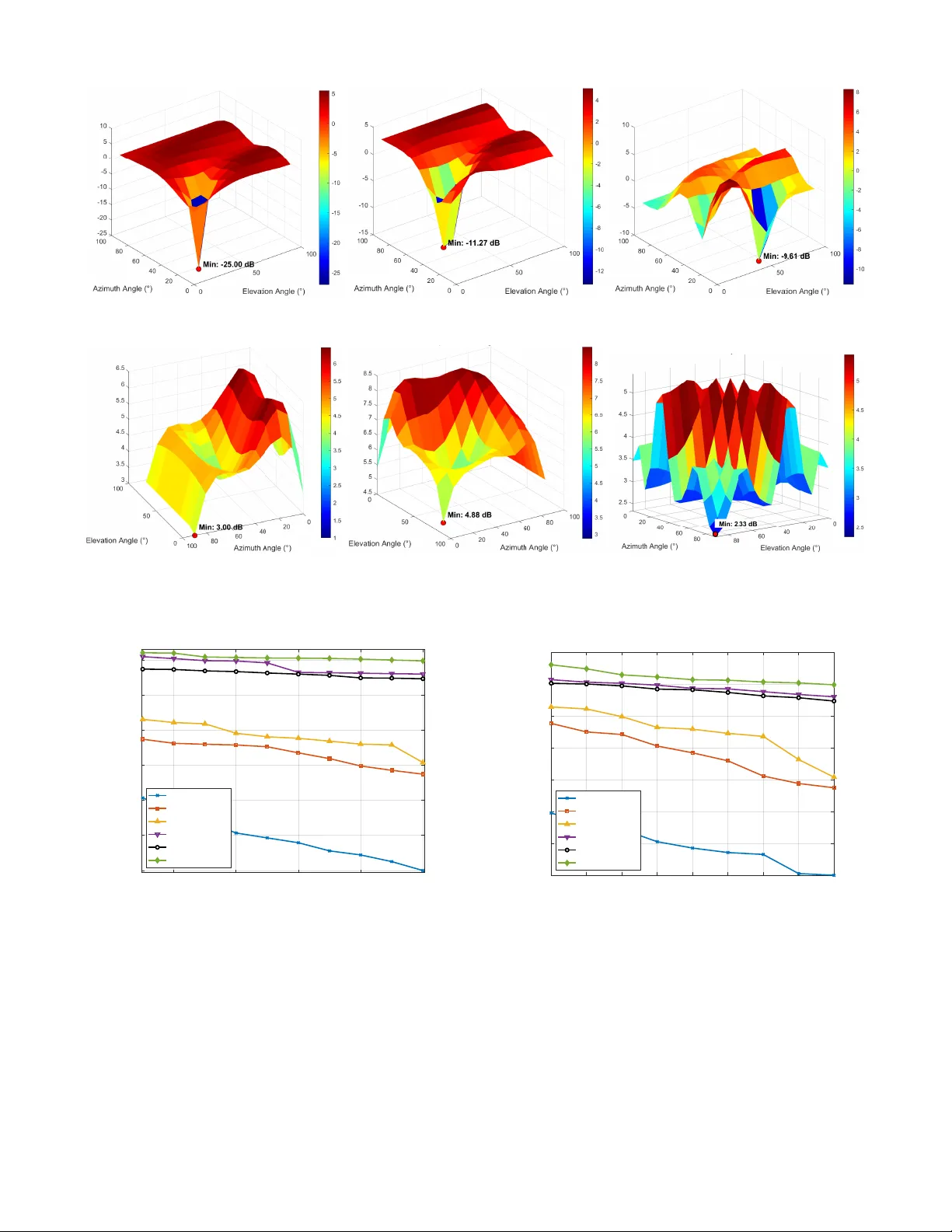
Comments & Academic Discussion
Loading comments...
Leave a Comment