Unveiling Hidden Convexity in Deep Learning: a Sparse Signal Processing Perspective

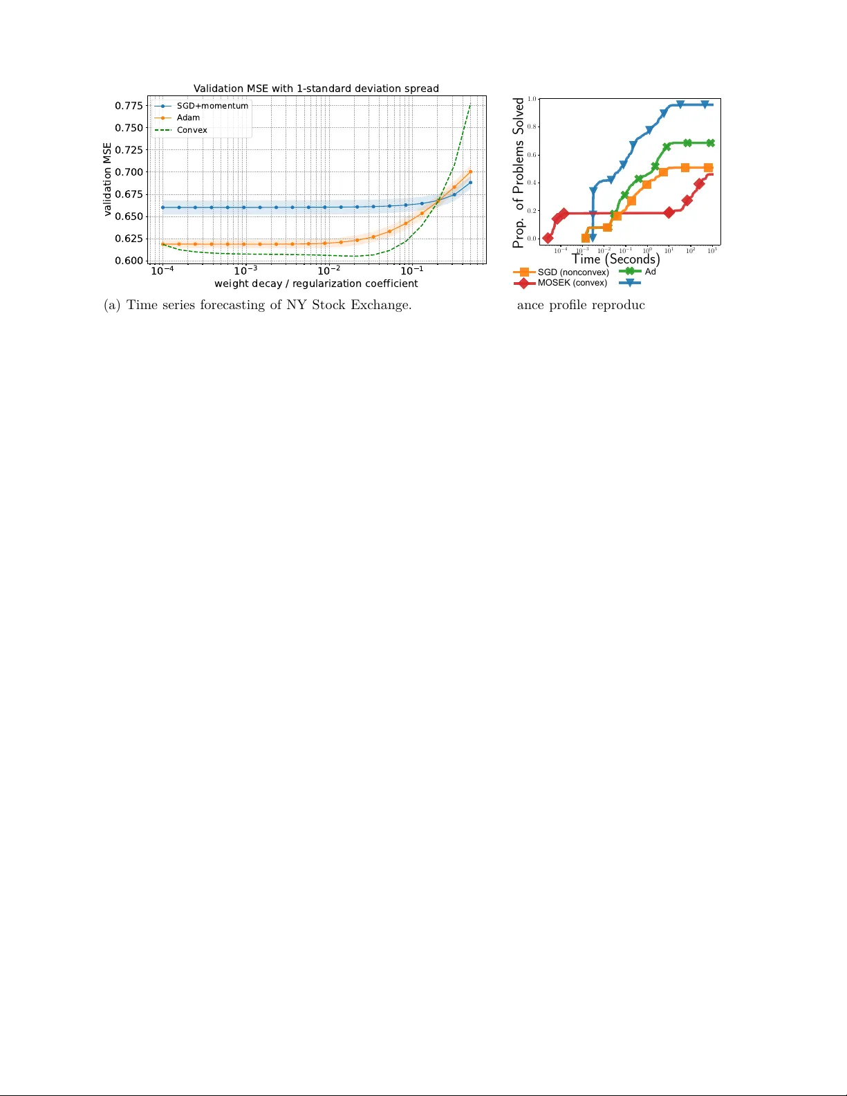
1 Un v eiling Hidden Con v exit y in Deep Learning: A Sparse Signal Pro cessing P ersp ectiv e Emi Zeger and Mert Pilanci Departmen t of Electrical Engineering, Stanford Univ ersit y In tro duction Deep neural net w orks (DNNs), particularly those using Rectied Linear Unit (ReLU) activ ation functions, ha v e ac hieved remarkable success across div erse machine learning tasks, including image recognition, audio pro cessing, and language mo deling [1]. Despite this success, the non-conv ex nature of DNN loss functions complicates optimization and limits theoretical understanding. These c hallenges are esp ecially p ertinent for signal processing applications where stability , robustness, and in terpretabilit y are crucial. V arious theoretical approac hes ha ve b een developed for analyzing neural netw orks (NNs). In this pap er, w e highligh t how recently developed conv ex equiv alences of ReLU NNs and their connections to sparse signal pro cessing mo dels can address the c hallenges of training and understanding NNs. Recen t researc h has unco v ered several hidden con vexities in the loss landscap es of certain NN arc hitectures, notably t w o-la y er ReLU net w orks and other deep er or v aried arc hitectures. By reframing the training pro cess as a conv ex optimization task, it b ecomes p ossible to eciently nd globally optimal solutions. This approach oers new p ersp ectives on the netw ork’s generalization and robustness c haracteristics while facilitating interpretabilit y . Leveraging Lasso-type mo dels and structure-inducing regularization frameworks, which are fundamen tal to ols in sparse representation mo deling and compressed sensing (CS), NN training can b e approached as a con vex optimization problem, enabling the interpretation of b oth globally and lo cally optimal solutions. This pap er seeks to provide an accessible and educational o verview that bridges recen t adv ances in the mathematics of deep learning with traditional signal pro cessing, encouraging broader signal pro cessing applications. The pap er is organized as follo ws. W e rst give a brief bac kground on NNs and approac hes to analyzing them using conv ex optimization. W e then present an equiv alence theorem b et w een a t w o-la y er ReLU NN and a conv ex group Lasso problem. W e describ e how deep er net w orks and alternative arc hitectures can also b e formulated as con v ex problems, discuss geometric © 2026 IEEE. P ersonal use of this material is p ermitted. Permission from IEEE must b e obtained for all other uses, in any curren t or future media, including reprinting/republishing this material for advertising or promotional purp oses, creating new collective works, for resale or redistribution to servers or lists, or reuse of any copyrigh ted comp onen t of this w ork in other works. March 26, 2026 DRAFT insigh ts, and present exp erimental results demonstrating p erformance b enets of training NNs as con v ex mo dels. Finally , we discuss remaining challenges and research directions for conv ex analysis of NNs. Related tutorial literature: A num b er of recen t works touch on asp ects of regularized neural netw ork training from a signal pro cessing p ersp ective. One suc h line of work, b y Parhi and No wak [2], studies neural weigh t balancing, analyzing ho w parameter magnitudes are distributed under a xed total ℓ 2 norm constrain t. While this viewp oint is related to the conv ex duality formulations referenced here, the present article adopts a broader p ersp ective that brings together multiple conv ex formulations and highlights their implications across a range of neural net work mo dels and learning settings. A distinct and complementary direction, explored in Sun et al. [3], in v estigates how regularization and the addition of sp ecial neurons can mak e the loss landscap e b enign, where lo cal minima are globally optimal. While regularization is also key to improving the loss landscap e in the present pap er, we fo cus on approaches to guaran tee that the NN loss is not just b enign, but conv ex. Notation: Denote 1 as the vector of ones and [ n ] = { 1 , · · · , n } . The Bo olean function 1 { x } returns 1 if x is true, and 0 otherwise. F unctions and op erations such as 1 { x } , ≥ , and activ ations σ ( x ) apply elemen t-wise to v ector inputs. The d × d iden tit y matrix is I d . There are m hidden neurons and n training samples x ( i ) ∈ R d , which are stac k ed column-wise into the data matrix X ∈ R d × n of rank r . NNs f : R d → R are dened for column vectors and extend to data matrix inputs as f ( X ) = ( f ( x (1) ) , · · · , f ( x ( n ) )) T . Bac kground: Neural netw orks NNs are parameterized functions used for sup ervised learning, comp osed of functions called neurons: f neuron ( x ) = σ ( x T w ) (1) mapping a vector input to a scalar, where w ∈ R d is a weigh t parameter and σ : R → R is a nonlinear activ ation function. A common activ ation function is the Rectied Linear Unit (ReLU): σ ( x ) = max { x, 0 } . An activ ation function is active at x if σ ( x )  = 0 . The activ ation σ is (p ositively) homogeneous (of degree one) if σ ( ax ) = aσ ( x ) for a > 0 [4]. F or example, non-negative inputs activ ate a ReLU. The nonlinearit y of an activ ation function distinguishes a neuron from a traditional linear mo del. The neuron (1) is inspired by a biological neuron in the brain, whic h receives synaptic inputs (represented by x ) whose intensities are mo dulated by the n um b er of receptors ( w ), and then res action p otentials as outputs. In the brain, neurons can op erate in series, feedback, and parallel pathw ays [5]. Motiv ated by these biological features, a hidden lay er consists of m parallel neurons: f lay er : R d → R 1 × m , f lay er ( x ) = σ ( x T W ) , (2) where W ∈ R d × m is called a weigh t matrix. An L -lay er NN consists of comp osing L − 1 nonlinear hidden lay ers (2), follow ed by a linear output lay er. The depth is L , and the width of a lay er is the n um b er of neurons in that la y er. A standard tw o-lay er NN f : R d → R takes the form f ( x ) = σ ( x T W ) α (3) where (2) is the rst hidden la y er of (3), and α ∈ R m is the weigh t vector of the outer linear lay er. Bias parameters can b e added implicitly by appending a 1 to x and an extra row to W . An L-la yer NN is said to b e shallow if L = 2 and deep if L > 2 . The NN (3) is a tw o-lay er, fully connected, feed-forw ard net w ork. There are man y t yp es of NNs consisting of v ariations on (3), as well as deep er net w orks. NNs t data to lab els/targets based on known pairs ( x (1) , y 1 ) , · · · , ( x ( n ) , y n ) that are given, where y i ∈ R is the target of training sample x ( i ) . A NN is trained by nding parameters (w eigh ts and biases) so that f ( x ( i ) ) ≈ y i , formulated as a training problem min θ ℓ ( f ( X ) , y ) + R ( θ ) (4) where X ∈ R d × n con tains x ( i ) as columns, y ∈ R n con tains y i , ℓ is a con vex loss function quantifying the error of the NN t, and θ is the parameter set, e.g., θ = { W , α } for tw o-lay er NNs (2). R is a regularization function that p enalizes large parameter magnitudes, encouraging simpler solutions, and will b e sp ecied for each NN. The training problem (4) is non-conv ex due to the pro duct of inner and outer w eigh ts. This p oses a ma jor challenge for analyzing NNs. T raditional approac hes to train NNs inv olve gradient descent algorithms, but these metho ds can conv erge to sub optimal lo cal minima. In con trast, if the training loss is conv ex, all stationary p oints would b e globally optimal. The next section discusses approac hes to improv e the loss landscap e. Impro ving the Loss Landscap e Bey ond reducing training complexity , regularization can also impro v e the geometry of the training ob jectiv e, or loss landscap e. In this context, a common goal is to enforce b enign b ehavior, meaning that optimization methods are less lik ely to encounter undesirable stationary p oints. A represen tative example, survey ed in [3] and references therein, shows that augmenting a netw ork with additional “sp ecial” neurons together with appropriate regularization can eliminate sub optimal lo cal minima (under suitable assumptions). These ideas extend b ey ond binary classication to m ulticlass and regression settings, and illustrate how arc hitectural mo dications and regularization can join tly shap e the loss landscap e. W e refer the reader to [3] for precise statements and conditions. Computational Complexity A well-kno wn result is that the global optimization of t w o-la y er ReLU NNs requires exp onential complexit y in the input dimension d (see e.g. [6] and the references therein). A relativ ely less kno wn result is that, even for xed d , training is NP-hard, implying no known p olynomial-time algorithm exists unless P = NP [6]. How ever, this hardness result applies sp ecically to unregularized training. In contrast, as discussed b elo w, conv ex formulations for netw orks incorp orating v arious regularizations can circumv ent NP-hardness, achieving p olynomial-time complexity for xed d [7]. While the conv ex formulations remain computationally demanding in high-dimensional settings, randomized approximation schemes [8] related to 1-bit compressed sensing [9] can guarantee near- global optimality . In addition to conv ex approximations, exact con v ex formulations for NNs enjoy close connections to sparse signal pro cessing. The next section reviews some of these signal processing metho ds. Bac kground on Sparse Signal Pro cessing, Compressed Sensing, and Geometric Algebra Sparse signal processing analyzes signals that admit a sparse representation in some basis or dictionary . Suc h sparsity enables ecient storage, transmission, and pro cessing of signals. A key application of sparse signal processing is CS [10, 11], which studies how sparse signals can b e reco v ered from far fewer measuremen ts than traditionally required by Nyquist sampling theory . V arious algorithms suc h as matching pursuit achiev e sparsity; we fo cus on Lasso-like mo dels for their connection to NNs. Lasso The Least Absolute Shrinkage and Selection Op erator (Lasso) [12] is a conv ex mo del widely used in sparse signal processing. Lasso p erforms v ariable selection and regularization sim ultaneously , making it an eective to ol for sparse representation in CS applications. The Lasso optimization problem is: min z 1 2 ∥ Az − y ∥ 2 2 + β ∥ z ∥ 1 (5) where A is the measuremen t (or dictionary) matrix whose columns A ( i ) ∈ R n are called feature v ectors or dictionary atoms, y ∈ R n is the observ ation vector, z ∈ R d and β > 0 is a regularization parameter controlling the sparsit y , i.e., the num b er of non-zero elements in a solution for z . The ℓ 1 -norm ∥ z ∥ 1 induces a sparse supp ort of z by p enalizing the absolute sum of the co ecients. In CS, Lasso serves as a con v ex relaxation of the NP-hard ℓ 0 -norm minimization problem, providing an ecien t computational framew ork for inducing sparse representations and v ariable selection with theoretical guarantees under certain conditions on the measurement matrix A . Group Lasso Group Lasso generalizes Lasso to promote sparse represen tations at the group level [13]. In many signal pro cessing applications, signals exhibit group sparsity , where non-zero co ecients o ccur in clusters. Group Lasso accounts for this structure by grouping v ariables and using an ℓ 1 /ℓ 2 -norm regularization: min z 1 2 ∥ Az − y ∥ 2 2 + β G X g =1 ∥ z ( g ) ∥ 2 (6) where z ( g ) denotes the co ecients in group g , G is the num b er of groups, and ∥ z ( g ) ∥ 2 is the ℓ 2 - norm of the group co ecients. This encourages entire groups of co ecients to b e zero, promoting structured sparsity that aligns with the underlying signal characteristics. When each group contains a single coecient z i , the term P G g =1 ∥ z ( g ) ∥ 2 = P j | z j | reduces to the ℓ 1 -norm, reco v ering the standard Lasso. Lasso and group Lasso mo dels are used in CS, describ ed next. Compressed Sensing (CS) Let z ∈ R d b e an unknown signal that we can indirectly observ e through linear measurements y i = z T a ( i ) (7) where a ( i ) ∈ R d are known measurement vectors. This yields a system of equations Az = y where the measuremen t matrix A ∈ R M × d has ro ws a T ( i ) and the observ ation vector y ∈ R M con tains corresp onding observ ations y i . W e choose the measurement vectors a T ( i ) and the num b er of measure- men ts M . If M = d and the measurement v ectors a ( i ) are linearly indep endent, then z = A − 1 y can b e uniquely reco v ered. How ever, in man y applications (suc h as MRI image reconstruction), each measuremen t incurs costs suc h as latency or nancial exp ense. CS estimates z from fewer than d measuremen ts, eectively compressing the signal by pro jecting it onto measurement vectors. The measuremen t vectors can b e random, e.g., a ( i ) ∼ N (0 , I d ) [11]. With fewer than d measurements, m ultiple candidate solutions satisfy Az = y ; CS selects a parsimonious solution by solving a Lasso (5) or group Lasso (6) dep ending on the sparsity structure of z . A v arian t, 1 -bit compressive sensing [9], uses quan tized measurements y i = Q ( z T a ( i ) ) , where Q ( x ) = sign ( x ) ∈ {− 1 , 1 } , compressing eac h measurement to only one bit of information. Solving min z ∥ z ∥ 1 s.t. Diag ( y )( Az ) ≥ 0 , ∥ z ∥ 2 = 1 reco v ers z , where the ℓ 2 constrain t resolves ambiguit y in the solution. Both CS and 1-bit CS mo dels connect deeply to conv ex NNs as w e will show in future sections. A tomic norm theory [14] views a ( i ) ∈ A as “atoms,” where A is the set of candidate atoms, and chooses z i b y minimizing the Mink o wski functional (gauge) of the conv ex hull of A as inf { t > 0 : y ∈ t conv( A ) } . This denes the atomic norm when A is symmetric ( − a ( i ) ∈ A if a ( i ) ∈ A ) and reduces to minimizing ∥ z ∥ 1 if A is nite. Conv ex NN formulations [7, 15–17] that will b e discussed t into an atomic norm p ersp ectiv e that views neuron outputs as atoms and outer-lay er weigh ts as co ecien ts z i . Conv ex formulations use ℓ 1 or group ℓ 1 p enalties, which represent atomic norm regularization that promotes a nite or sparse set of active neurons. Nuclear Norm Regularization The nuclear norm of a matrix W is the ℓ 1 -norm of its singular v alues: ∥ W ∥ ∗ = P r k =1 σ k ( W ) = ∥ σ ( W ) ∥ 1 , where r is the rank of W [18]. As a sp ecial case, the nuclear norm of a positive semidenite matrix is its trace. The n uclear norm is often used in optimization problems to search for lo w-rank matrices [18]. W e discuss tw o examples, robust PCA and matrix completion. Con v exit y w.r.t: Approac h Motiv ation/T echnique Relation to SP outer-la y er w eigh ts [15] column generation b o osting matc hing pursuit parameters [7] con v ex duality , Lasso h yp erplane arrangements zonotop es sparse recov ery , 1-bit CS [9] probabilit y measures [23, 24] mean eld in tegration neural tangent k ernel (NTK) [25] k ernel metho ds [26] net w ork output [4] shift complexity to regularization matrix factorization, n uclear norm [18] CS: robust PCA [20] matrix completion [19] quan tized w eigh ts [27] linear program in tersection graph analysis graphical mo dels [28] T ABLE I: Comparison of con v ex p ersp ectives on NNs. Each approach is motiv ated by , or inv olves, tec hniques related to signal pro cessing (SP). The approaches in the rst tw o ro ws also inv olve ℓ 1 regularizations, linking them to sparse representations in signal pro cessing. 1) Robust PCA: The robust Principal Comp onent Analysis (PCA) problem [19] for a matrix X is min W , S : X = S + W ∥ W ∥ ∗ + β ∥ S ∥ 1 . (8) The robust PCA problem is a conv ex heuristic to decomp ose X into the sum of a low-rank matrix W and a sparse matrix S b y p enalizing the singular v alues of W and all elemen ts of S . The lo w-rank matrix W can represent the underlying low-dimensional subspace and the sparse matrix S represents outliers. 2) Matrix completion: The matrix completion problem [20] is as follows. Given a n × n matrix where only some of the v alues are known, ll in the rest of the matrix so that it has the low est rank p ossible, consistent with the given elemen ts. This problem can b e appro ximately solved by lling in the unknown v alues that give the low est n uclear norm [20]. Geometric Algebra Geometric (Cliord) algebra is a mathematical framework that generalizes complex num b ers to higher-dimensional v ector spaces, including quaternions and hypercomplex num b ers. It provides a unied wa y to represent and p erform op erations on geometric objects [21]. Recen t work has applied geometric algebra to develop new signal pro cessing techniques for image, audio, and video pro cessing [22], as well as deep learning by leveraging geometric representations to enable more compact and expressive models [22]. The following sections relate signal pro cessing methods to con v ex optimization of NNs. A conv ex view of shallo w neural netw orks Since conv ex functions hav e b een well-studied theoretically , one ma jor approach to study NNs is to reformulate them via con v ex optimization. Suc h conv ex formulations provide v aluable intuition in to the underlying structure of optimal netw ork weigh ts and the asso ciated mo del classes. They enable rigorous analysis of optimality guarantees, principled stopping criteria, numerical stabilit y , and reliabilit y—all critical features for mission-critical applications common in signal pro cessing, suc h as real-time control systems in autonomous v ehicles, p ow er grid management, and healthcare monitoring. Moreov er, con v ex programs mak e training NNs agnostic to hyperparameters suc h as initialization and mini-batching, whic h often exert a signicant inuence on the p erformance of lo cal optimization metho ds. W e discuss v arious approaches to represent NN training problems as conv ex problems. This section assumes the netw orks are tw o-lay er ReLU netw orks unless otherwise stated. Deep er netw orks follow in later sections. Con v exit y with Resp ect to the Outer-La y er W eigh ts Bengio et al. [15] and Bach [16] show that training a tw o–lay er, innitely wide NN with a conv ex loss and sparsity-promoting regularization on the outer la y er can b e cast as a conv ex optimization problem. (In their setup, an ℓ 1 norm is immediate when the hidden-unit set is countable.) Let Φ =  σ ( X T w ) : w ∈ R d  denote the (uncountable) set of hidden–lay er outputs ev aluated on the training data matrix X ∈ R d × n . T raining reduces to selecting outer-lay er weigh ts α by solving [15, 16] min α ℓ  Z Φ ϕ dα ( ϕ ) , y  + ∥ α ∥ TV , (9) where ℓ is any conv ex loss, the integral in tegrates o ver all p ossible ϕ ∈ Φ ⊂ R n , the nal-lay er w eigh t α : Φ → R is a nite signed Radon measure on Φ so that R Φ ϕ dα ( ϕ ) ∈ R n is w ell-dened, and the regularization is the total v ariation norm [ 16]. While [16] develops a function-space analysis of (9) by viewing the outer-lay er weigh ts as a signed measure ov er a contin uous feature family and regularizing its total v ariation, the earlier w ork [15] highlights that the sparsity p enalty admits an optimal solution supp orted on nitely many hidden units (at most n + 1 , b y their Theorem 3.1). In this case, the NN reduces to a discrete and nite linear combination of features ϕ , the con tin uous distribution α ( ϕ ) in (9) is identied with a vector of co ecients α ∈ R m , and the regularization ∥ α ∥ TV simplies to the usual ℓ 1 -norm penalty . Bengio et al. [15] adopts a column generation strategy to optimize this NN: b egin with an empt y hidden la yer and iterativ ely (i) iden tify the neuron that most improv es the ob jective and add it to the hidden lay er (ii) re‐optimize (9) ov er the current co ecien ts. Step (i) consists of solving a weigh ted linear classication problem, which is non‐conv ex in general. With hinge loss, the pro cedure is shown to reach a global optim um in at most n + 1 iterations, corresp onding to n + 1 neurons [15]. This incremental scheme links NNs to b o osting—b oth build predictors by sequentially adding simple comp onents—and, more broadly , to greedy approximation metho ds in signal pro cessing (e.g., matching pursuit and related pro cedures) [29]. The extension to contin uous distributions in [16] also connects naturally to F rank–W olfe st yle incremental metho ds. The main computational b ottleneck is the non‐conv ex subproblem used to insert eac h neuron, which remains c hallenging in high dimensions. F rom a signal processing p ersp ectiv e, the features ϕ ∈ Φ can b e viewed as basis functions for the netw ork [16]. The approach in [16] is used to analyze generalization prop erties of innite-width, t wo-la yer NNs with homogeneous activ ations. Con v exit y with Resp ect to the Net w ork Output In this section we review the con v ex formulation in tro duced by Haeele and Vidal [4]. Their central idea is to treat the en tire netw ork output as the decision v ariable, which con v erts the learning task in to a conv ex optimization problem. Accordingly , the tw o–lay er netw ork in (3) can b e rewritten as f ( x ) = m X i =1 σ  x T w ( i )  α i (10) where w ( i ) ∈ R d is the i th column of weigh t matrix W ∈ R d × m (2). F or a wide class of regularization functions R ( θ ) including norm p enalties, the training problem (4) is equiv alent to the conv ex problem min F ∈ R n ℓ ( F , y ) + ˜ R ( F ) (11) where ˜ R ( F ) is the minimum parameter regularization such that the corresp onding net w ork outputs F [4]: ˜ R ( F ) = min θ R ( θ ) s.t. f ( X ) = F (12) The mo died regularization ˜ R (12) is con v ex [4], making (11) con v ex. In contrast to [4], the con v ex problem (11) is nite-dimensional, as the optimization v ariable F is nite-dimensional. This con v ex reformulation shifts the complexit y from optimizing ov er all w eigh ts to optimizing the regularization term. The approach in [4] is motiv ated by matrix factorization, as follows. Supp ose A ∈ R d 1 × r , B ∈ R r × d 2 , Y ∈ R d 1 × d 2 , where Y , d 1 , d 2 are kno wn and A , B , r are unkno wn. The matrix factorization problem min r, A , B 1 2 ∥ AB − Y ∥ 2 F + β ( ∥ A ∥ 2 F + ∥ B ∥ 2 F ) where the loss function b et w een the matrices is ℓ ( Z , Y ) = 1 2 ∥ Z − Y ∥ 2 F and the regularization is R ( A , B ) = β ( ∥ A ∥ 2 F + ∥ B ∥ 2 F ) , can b e analyzed similarly to (11) as min F ∈ R d 1 × d 2 1 2 ∥ F − Y ∥ 2 F + ˜ R ( F ) where similarly to (12), the mo died regularization is ˜ R ( F ) = min r, A , B β ( ∥ A ∥ 2 F + ∥ B ∥ 2 F ) s.t. AB = F F or matrix factorization, this mo died regularization turns out to b e the nuclear norm: ˜ R ( F ) = ∥ F ∥ ∗ , a regularization employ ed in sparse signal pro cessing (see Nuclear Norm Regularization ab ov e) [4]. Ho w ev er, for general NNs, the denition of ˜ R ( F ) (12) is not explicit and leav es (11) intractable. Despite this limitation, conv exity enables useful theoretical insigh ts. Consider an augmen ted training problem where the netw ork is expanded to include one more neuron. A lo cal optimum of the original training problem is globally optimal if adding a neuron with zero-v alued weigh ts is lo cally optimal in the augmented training problem [4]. In particular, the loss landscap e is b enign [3] if for some i ∈ [ m ] , the i th parameters are zero: w ( i ) = 0 , α i = 0 in (10) [4]. This p ersp ective on b enign landscap es via the addition of neurons is related to the approac hes discussed in [3]: see Impro ving the Loss Landscap e ab ov e. Building o of the b enign landscap e results, [4] describ es an algorithm to nd a globally optimal NN b y repeating a lo cal descen t step that nds a lo cal optimum and an expansion step that adds another neuron to the NN. A lo cal descent path is a sequence of parameter v alues with a non-increasing ob jectiv e in the non-conv ex training problem. If the net w ork starts with at least n neurons (i.e., the n um b er of training samples), a lo cal descent path to a global optimum exists [4]. F or a suciently smo oth and strongly conv ex ob jectiv e, gradient descent with suciently small step size would b e an example of lo cal descen t [4]. Ho w ev er, for non-con v ex problems, nding a local descent path can b e NP-hard [4]. In addition, the upp er b ound on the n um b er of neurons needed to guarantee a lo cal descent path can b e large for practical algorithms [4]. A future area of w ork is to analyze cases where this can b e reduced [4]. Con v exit y with Resp ect to Probability Measures A complemen tary route is to lift the inner parameters and optimize ov er a probabilit y distribution on weigh ts (see e.g. Bach and Chizat [23], Mei et al. [24]). The starting p oint is to express a nite t w o-la yer netw ork of width m as an exp ectation. If p m denotes the empirical measure that assigns mass 1 /m to each parameter pair ( w ( i ) , α i ) , then a 2 -lay er NN can b e represented as f m ( x ) = 1 m m X i =1 σ  x T w ( i )  α i = E ( w ,α ) ∼ p m  σ ( x T w ) α  (13) where w ( i ) , w ∈ R d and α i , α ∈ R . Letting the width m → ∞ while k eeping the parameters bounded, the discrete measures p m con v erge (along subsequences) to a probabilit y distribution p on R d +1 . The netw ork output conv erges accordingly to the mean-eld expression f p ( x ) = Z σ ( x T w ) α d p ( w , α ) . (14) Because f p ( x ) dep ends linearly on p , an y conv ex loss ℓ  f ( X ) , y  yields a conv ex training problem min p ∈P ℓ  f p ( X ) , y  , o v er probability measures, where P denotes the set of all non-negative Borel measures on R d +1 whose total mass is one. Therefore, the training problem is revealed as a conv ex optimization in function space. Kernel (lazy-training) Regime and the Neural T angent Kernel Let ϕ m ( x ) =  σ ( x T w (1) ) , . . . , σ ( x T w ( m ) )  T . If we sample the inner w eigh ts i.i.d. from a random distribution, then freeze them and optimize only the outer coecients, optimizing the discrete mean– eld mo del (13) reduces to linear regression: min α 1 2   y − 1 m ϕ m ( X ) T α   2 2 . Gradient descent for this problem is kno wn as kernel gradien t descent with empirical kernel ˆ k m ( x , x ′ ) = 1 m ϕ m ( x ) T ϕ m ( x ′ ) . As the width m tends to innit y the empirical k ernel ˆ k m ( x , x ′ ) = 1 m P m i =1 σ ( x T w ( i ) ) σ ( x ′ T w ( i ) ) con v erges to a deterministic limit k RF ( x , x ′ ) , where the subscript ‘RF’ denotes that this limit stems from random features. Jacot et al. [25] sho w that if one trains the full netw ork but stays in the lazy-training regime, the Jacobian of the loss sta ys nearly constant and training is equiv alen t to k ernel gradient descent with a (generally dieren t but related) limiting kernel k NTK ( x , x ′ ) , called the Neural T angen t Kernel (NTK). The NTK connects NNs to kernel metho ds, a to ol used in signal pro cessing to lift signals into higher dimensions for linear separation, among other applications [26]. Con v exit y via Quantization and Polyhedral Representations In another approach, Bienstock et al. [27] shows that a linear program can approximate NN training through weigh t quantization and p olyhedral representations. This formulation assumes the training data lies within the b o x [ − 1 , 1] d , and then quantizes the data and weigh ts to nite num b ers of bits. This transforms the training problem into an optimization program with a linear ob jective, binary v ariables, and linear constraints, known as a binary program. An intersection graph represen ts the optimization v ariables of the binary program as no des, and the constraints as edges b et ween them. Relaxing the binary v ariables to con tinuous v ariables conv erts the binary program into a linear program. The treewidth of the intersection graph measures how closely the graph resembles a tree, dened as the minimal width among all p ossible tree decomp ositions of the graph. This treewidth c haracterizes the computational complexity inv olved in solving the linear program. Specically , the binary program analyzed in [27] p ossesses low treewidth, leading to a linear program whose constrain ts gro w linearly with the num b er of training samples. Therefore, global NN training can b e appro ximated via low treewidth optimization. T reewidth indicates the sparsit y of the intersection graph relativ e to a tree structure, with exact trees ha ving the lo west treewidth. In general, structured sparsit y simplies optimization; in this case, tree-structured sparsit y restricts supp orts to ro oted subtrees (connected subgraphs) of a tree. Such signal represen tations arise in graphical mo dels for image and graph signal pro cessing [28], and decision or regression tree mo dels [29]. Although these problems are not t ypically expressed with explicit constrain ts, they are often formulated as optimization problems that induce implicit intersection graphs capturing paren t-child branch dep endencies among the signal comp onents. NNs ma y therefore b e interpreted as lo oser relatives of tree-sparse mo dels with richer parameter interactions that still preserve tractability prop erties asso ciated with lo w treewidth. In [27], the p olyhedral constrain t set captures the NN structure. T raining on dierent datasets corresp onds to solving linear programs constrained b y distinct faces of this p olyhedron. Imp ortantly , this linear program representation do es not require the loss function to b e conv ex. This approach applies to b oth unregularized and regularized training, including weigh t norm p enalties as regularization. Con v exit y with Resp ect to the Net w ork Parameters The previous sections describ e approaches that cast training problems as implicit conv ex programs, either in terms of the netw ork output or hidden lay er activ ations, or b y mo difying the w eigh ts through quantization, con tinuous distributions, or innite-width limits. In contrast, a line of recent w ork [7, 21] introduces explicit conv ex formulations that establish direct corresp ondences b et w een the v ariables of the conv ex programs and the netw ork weigh ts. These formulations inv olve a nite n um b er of optimization v ariables, making them more representativ e of NNs in practice. These conv ex mo dels closely parallel sparse mo deling metho ds in signal pro cessing such as Lasso, group Lasso, one-bit CS, and n uclear-norm-based matrix completion. This conv ex approac h unco vers certain v ariable selection prop erties of w eigh t-deca y regularization, a characteristic of NNs also studied in [16]. Building on these ideas, Bai et al. [8] dev elops an adversarial training strategy , while Prakhy a et al. [30] constructs semidenite relaxations for vector-output, tw o-lay er ReLU net w orks with ℓ 2 regularization. The mathematical proof tec hniques used in the pro ofs of these results are conv ex analytic in nature, and include conv ex geometry , p olar duality and analysis of extreme p oints. W e explore the key elements of this conv ex equiv alence, starting with tw o-lay er netw orks. Explicit Conv ex Programs for T wo-la yer Net w orks This section examines tw o-lay er NNs with scalar outputs and ReLU activ ations: f ( x ) =  x T W  + α , (15) and presents an equiv alent Lasso-type explicit formulation of the training problem that establishes a connection b etw een sparsity-inducing signal pro cessing and NNs. The Lasso equiv alence gives b oth practical approaches for training and theoretical insights in to NN represen tation p ow er through ideas from signal pro cessing. The training problem (4) for the netw ork (15) using ℓ 2 loss and ℓ 2 regularization is min W , α 1 2 ∥ f ( X ) − y ∥ 2 2 + β  ∥ W ∥ 2 F + ∥ α ∥ 2 2  . (16) The term ∥ W ∥ 2 F + ∥ α ∥ 2 2 represen ts w eigh t deca y regularization. W e will recast the non-con vex training problem as a con v ex group Lasso problem via hyperplane arrangements, which we dene next. x (1) x (2) x (3) x (4) w x (2) x (3) w K h = h 0 1 1 0 i T X = h x (1) x (2) x (3) x (4) i Fig. 1: Illustration of a separating hyperplane (left plot) and an activ ation cham b er (righ t plot). Hyp erplane Arrangement Patterns A h yp erplane arrangement is a nite collection of hyperplanes in a giv en vector space. F or simplic- it y , w e rst consider h yp erplane arrangements in R 2 . In R 2 , a separation pattern or hyperplane arrangemen t pattern of a dataset is a signed partition of the data b y a line through the origin, called a separating line. A separation pattern is represen ted by a vector h ∈ { 0 , 1 } n , where n is the n um b er of training samples. Sp ecically , h is a separation pattern if there exists a separating line suc h that each data p oin t x ( i ) is assigned h i = 0 if it lies on one side of the line and h i = 1 if it lies on the opp osite side. Each separating line has an asso ciated orthogonal vector whose orien tation determines which side corresp onds to h i = 0 versus h i = 1 . The orthogonal vectors asso ciated with separating lines that giv e rise to the same separation pattern form a cone, called an activ ation c ham b er; an example is given b elow. Example: Consider 2-D training data x (1) , x (2) , x (3) , x (4) sho wn in the left plot of Figure 1. An example of a separation (or h yp erplane arrangement) pattern is h = (0 , 1 , 1 , 0) T . This separation pattern corresp onds to x (2) and x (3) b eing on the same side of a separating line of the form w T x = 0 . As shown in the gure, x (2) , x (3) lie on the side of this line in the direction of w (halfspace shaded in purple), and x (1) , x (4) are on the other side. In the righ t plot, the magen ta-shaded activ ation cham b er K illustrates the cone of all p ossible vectors w that are orthogonal to separating lines pro ducing pattern h . The red and blue regions are the halfspaces x T (2) w ≥ 0 and x T (3) w ≥ 0 , respectively , and the c hamber K is their intersection. The hyperplane arrangemen t denitions extend to higher dimensions by considering separating hyperplanes instead of separating lines. The set of hyperplane arrangemen t patterns of a data matrix X ∈ R d × n is H = n 1 { X T w ≥ 0 } : w ∈ R d o . (17) T raining data on the p ositiv e side of the hyperplane X T w = 0 satisfy x T w ≥ 0 and th us activ ate the neuron ( x T w ) + , while those on the negative side do not. The num b er of patterns is |H | ≤ 2 r  e ( n − 1) r  r , where r = rank ( X ) ≤ min { n, d } and e = 2 . 718 ... denotes Euler’s constant [7]. Let G = |H| and en umerate the patterns as H = { h (1) , · · · , h ( G ) } . The activ ation cham b er for a pattern h ( g ) ∈ H is K ( g ) = { w ∈ R d : 1 { X T w ≥ 0 } = h ( g ) } , which is the cone of all weigh ts that induce an activ ation pattern h ( g ) . Here, g ∈ { 1 , · · · , G } is an integer index enumerating the h yp erplane arrangemen t patterns and asso ciated v ectors or matrices. The h yp erplane enco ding matrix is D ( g ) = Diag ( h ( g ) ) for g = 1 , · · · , G . F or xed X , a neuron’s output ( X T w ) + as a function of w is linear o ver w ∈ K ( g ) , as  X T w  + = D ( g ) X T w . The activ ation cham b ers partition R d = S G g =1 K ( g ) , and so the matrices D (1) , · · · , D ( G ) completely characterize the piecewise linearity of the neuron output ( X T w ) + . F or additional mathematical prop erties and a thorough introduction to the theory of hyperplane arrangemen ts, w e refer the reader to [31]. The training problem is equiv alen t to another optimization problem P if they share the same optimal v alue, and if an optimal netw ork to the training problem can b e reconstructed from an optimal solution to P . Theorem 1 ([7]). The non-con v ex training problem (16) with w eigh t decay regularization for a t w o-la yer ReLU netw ork is equiv alent to the conv ex group Lasso problem min u ( g ) , v ( g ) ∈K ( g ) 1 2 ∥ G X g =1 D ( g ) X T  u ( g ) − v ( g )  − y ∥ 2 2 + β G X g =1  ∥ u ( g ) ∥ 2 + ∥ v ( g ) ∥ 2  (18) where K ( g ) = { z ( g ) : (2 D ( g ) − I ) X T z ( g ) ≥ 0 } , pro vided the num b er of neurons satises m ≥ m ∗ where m ∗ is the num b er of non-zero u ( g ) , v ( g ) . Theorem 1 enables global optimization of ReLU NNs via conv ex optimization and an interpretation of the netw ork as a signal pro cessing mo del that promotes sparsit y , with the dictionary A = [ D (1) X T , ..., D ( G ) X T ] . The num b er m ∗ is a critical threshold on the n um b er of neurons (n um b er of columns of W ) necessary to allow the netw ork to b e suciently expressive to mo del the data. The group Lasso v ariable z ∈ R Gd is partitioned into G consecutive subv ectors z ( g ) = u ( g ) − v ( g ) ∈ R d , eac h corresp onding to a single neuron. Given an optimal solution to the group Lasso problem (18), the weigh ts for an optimal NN are w ( g ) = u ( g ) q ∥ u ( g ) ∥ 2 , α g = q ∥ u ( g ) ∥ 2 or w ( g ) = v ( g ) q ∥ v ( g ) ∥ 2 , α g = − q ∥ v ( g ) ∥ 2 (19) for all non-zero u ( g ) , v ( g ) . The w eight v ectors w ( g ) ∈ R d are columns of the weigh t matrix W ∈ R d × m and α g ∈ R are scalar comp onents of α ∈ R m . The Lasso v ariables u ( g ) and v ( g ) represen t weigh ts corresp onding to p ositive versus negative nal-lay er weigh ts α g . Example [32]: Consider the training data matrix X = h x (1) x (2) x (3) i = " 2 3 1 2 3 0 # . (20) Although there are 2 3 = 8 distinct binary sequences of length 3 , X has G = 3 hyperplane arrangement patterns in this case excluding the 0 matrix, as illustrated b elow from [32]. linear classier (2,2) (3,3) (1,0) x y linear classier (2,2) (3,3) (1,0) x y linear classier (2,2) (3,3) (1,0) x y D 1 =     1 0 0 0 1 0 0 0 1     D 2 =     1 0 0 0 1 0 0 0 0     D 3 =     0 0 0 0 0 0 0 0 1     Consider training a tw o-lay er ReLU NN on the data matrix in (20). F or an arbitrary lab el v ector y ∈ R 3 and the squared loss, the netw ork in the equiv alent conv ex program ( 18) is written piecewise linearly as f ( X ) = D (1) X T ( u (1) − v (1) ) + D (2) X T ( u (2) − v (2) ) + D (3) X T ( u (3) − v (3) ) . (21) This NN is in terpretable from a signal pro cessing p ersp ective [13]: it lo oks for a group sparse mo del to explain the response y via a mixture of linear mo dels u ( g ) − v ( g ) tuned to each activ ation c ham b er. The linear term u (2) − v (2) predicts on { x (1) , x (2) } , and u (3) − v (3) on { x (3) } , etc. Due to the regularization term P 3 g =1 ∥ u ( g ) ∥ 2 + ∥ v ( g ) ∥ 2 in (18), only a few of these linear terms will b e non-zero at the optim um, showing a bias to w ards simple solutions among all piecewise linear mo dels. The conv ex formulation therefore oers insights into the role of regularization in preven ting o v ertting. While the 2-D example (20) en umerates hyperplanes by hand, this b ecomes impractical in high dimensions and is addressed next. Computational Complexity of Global Optimization and Randomized Sampling for P olynomial-time Appro ximation: V arious approaches hav e analyzed the complexit y resulting from training NNs with a conv ex program. The complexity of solving the conv ex problem (18) is prop ortional to ( n d ) d , where n is the n umber of samples and d is the dimension of the input. Although the exp onential dep endence with resp ect to d is unav oidable, the complexity of (18) is p olynomial in the n umber of neurons and samples, which is signicantly low er than brute-force search ov er the linear regions of ReLUs ( O  2 md  ) [7]. By leveraging weigh t decay regularization, Theorem 1 ov ercomes the NP-hardness of unregularized NN training for xed d [6]. In [4], the maximum width needed for a tw o-lay er NN (trained with a broad class of regularizations) to reach global optimality corresp onds to the num b er of lo cal descent searches their algorithm must p erform, which is linear in n . Ho wev er, eac h lo cal descen t step can b e NP-hard [4]. Theorem 1 requires a sucient width of m ≥ m ∗ for the con vex equiv alence to hold. This is consisten t with [6], which sho ws that training has p olynomial time complexit y when the num b er of neurons exceeds a critical width, and can b ecome NP-hard otherwise. The exact width thresholds in [6] and Theorem 1 dier b ecause Theorem 1 considers parameter regularization but [6] do es not. In [27], p olytop es geometrically enco de discretized training problems, b oth with and without regularization. While [7] c haracterizes a NN for xed training data as an exact piecewise linear mo del dened ov er a collection of p olytop es that is exp onential in d and p olynomial in n , [27] shows that a single p olytop e, with a num b er of faces that is exp onential in d and linear in n , enco des appro ximations of training problems for all data sets in [ − 1 , 1] d . Sp ecically , training a netw ork on a given data set amounts to solving a linear program o v er a face of the p olytop e, up to an additive quan tization error [27]. Hyp erplane Arrangements and Zonotop es Fig. 2: Zonotop e example. Lines indicate normal cones. Hyp erplane arrangemen ts (17) can b e describ ed geometrically . Sp ecically , the hyperplane arrangement patterns of X corre- sp ond to v ertices of the zonotope (Figure 2) of X , dened as Z = Conv ( n X i =1 h i x ( i ) : h i ∈ { 0 , 1 } ) = { Xh : h ∈ [0 , 1] n } . (22) The corresp ondence is as follows [32]. Since Z is a p olytop e, for every w ∈ R d , there is a v ertex z ∗ of Z such that ( z ∗ ) T w = S ( w ) = max z ∈Z z T w . (23) The line z T w = ( z ∗ ) T w is a supp orting h yp erplane of Z , shown in Figure 3 of Sampling Arrangemen t Patterns b elo w, and S ( w ) is the supp ort function of Z . W e ha v e shown that v ertices maximize the supp ort function of Z . Conv ersely , for every vertex z ∗ , there is a w suc h that that z ∗ = arg max z ∈Z z T w . Now, (23) is equiv alent to max h i ∈ [0 , 1] n X i =1 h i x T ( i ) w whose solution is a hyperplane arrangement pattern h = 1 { X T w ≥ 0 } . Therefore eac h v ertex z ∗ corresp onds to an activ ation c ham b er { w : sign  X T w  = h } . The inset “Sampling Arrangemen t Patterns” discusses h yp erplane sampling to reduce computational complexit y . Bai et al. [8] presen ts and analyzes a pro cedure to sample a collection of h yp erplanes that scales linearly with n . As shown in [8], [32], it is p ossible to control the optimization error resulting from randomly sampling arrangement patterns for the Lasso problem. In particular, sampling O ( P log ( P )) random arrangement patterns yields a globally optimal solution with high probability , where P is the total num b er of hyperplane arrangement patterns [32]. In [ 33], it was prov en that the patterns can b e randomly subsampled to low er the complexit y to n d log n with a guaranteed √ log n relative appro ximation of the ob jectiv e. This enables fully p olynomial-time approximation sc hemes for the conv ex NN program. Sampling Arrangement Patterns 0 x 1 x 2 x 1 + x 2 h Fig. 3: Zonotop e normal cones Using a subset of hyperplane arrangement pat- terns (17) in the Lasso problem (18) can reduce the exp onential complexity of enumerating all patterns. This yields a subsampled Lasso prob- lem, and is prov en to corresp ond to station- ary p oints of the non-conv ex training problem [32]. A practical w a y to sample h yp erplane arrangemen t patterns is to generate random w ∼ N (0 , I d ) and ev aluate h ( g ) = 1 { X T w ≥ 0 } [7],[8]. Then D ( g ) = Diag ( h ( g ) ) are used to solv e an estimated group Lasso problem (18). An estimated optimal netw ork is reconstructed from the estimated Lasso solution via (19). The hyperplane sampling implicitly samples vertices of the data’s zonotop e, whose normal cone solid angles (Figure 3) are prop ortional to the probabilit y of sampling each vertex [32]. Zonotop es are described in (22) in the inset “Hyperplane Arrangements and Zonotop es” . Zonotop es hav e v arious signal pro cessing applications [34]. The h yp erplane sampling approach is directly connected to 1 -bit compressiv e sensing [9], whic h randomly samples a signal x ∈ R d as sign ( x T w ( i ) ) where w ( i ) = a ( i ) , x = z in (7). Multiple signals stack ed into a data matrix X can b e randomly sampled at once as sign  X T w  where w ∼ N (0 , I d ) , which is precisely sampling activ ation cham b ers, or equiv alen tly , the v ertices of a zonotop e. Sampling patterns is also related to Lo cality-Sensitiv e Hashing (LSH), a metho d for ecien tly nding nearest neighbors (in Euclidean distance) of an en try x ∈ R d in a database [35]. LSH places x in a database bin according to the sign of x T w where w ∼ N (0 , I d ) , similar to 1-bit CS. The group Lasso formulation in Theorem 1 enables mo del pruning algorithms to generate minimal mo dels [36]. A minimal model is a minimum-width, globally optimal NN. Starting an optimal con vex solution (18), [36] successively remov es ’redundan t’ neurons corresp onding to group Lasso v ariables u ( g ) whose contributions D ( g ) X T u ( g ) to the prediction are linear combinations of that from other group v ariables. The algorithm also extends to constructing approximate minimal mo dels that use few er neurons than required for global optimalit y [36]. The pro of of Theorem 1 in v olv es sho wing that the bidual of the non-conv ex training problem is equiv alent to the Lasso problem and reconstructing a netw ork from the Lasso problem that achiev es the same ob jective in the training problem as the Lasso problem, th us closing the dualit y gap and pro ving equiv alence. W e note that there are alternativ e w a ys to obtain the con vex formulation. One approach inv olves showing that neurons with the same arrangement pattern can b e merged and then optimizing ov er neurons constrained to the activ ation cham b ers. Here, we fo cus on the con v ex duality approach, which parallels the duality theory of traditional Lasso metho ds used in signal pro cessing. The next section describ es a neural w eigh t prop erty related to the pro of. Gaining Insigh t into Netw ork W eights: Optimal Neural Scaling. Y ang et al. [37] and P arhi and Now ak [2] describ e a “Neural Balance Theorem” for training with weigh t decay regularization. The theorem states that the magnitude of the input and output weigh ts of any neuron with homogeneous activ ation m ust b e equal, satisfying a “balancing constrain t. ” Sp ecically , the minimum-w eight representation of a given function b y a tw o-lay er NN satises | α j | = ∥ w ( j ) ∥ 2 for all j where w ( j ) if the j th column of W (3). The netw ork m ust hav e a homogeneous activ ation such as ReLU. This w eight scaling strategy is used as an imp ortan t rst step in the con vexication approach of [7]. The ReLU NN (10) f ( x ) = P m j =1 ( x T w ( j ) ) + α j is in v ariant to multiplying w ( j ) and dividing α j b y an y p ositive scalar γ j . On the other hand, for xed w ( j ) , α j , their training regularization ∥ γ j w ( j ) ∥ 2 2 + | 1 γ j α j | 2 is minimized o v er γ j when ∥ γ j w ( j ) ∥ 2 = | 1 γ j α j | , i.e., γ ∗ j = | α j | ∥ w ( j ) ∥ 2 . Therefore an optimal NN that minimizes the regularized training problem will hav e equal magnitude inner and outer weigh ts | α j | = ∥ w ( j ) ∥ 2 for all j . In tuitively , this means that an optimal net w ork balances w eigh ts evenly b etw een lay ers. Similar scaling prop erties hold for deep er netw orks and other activ ations. Next we discuss the deriv ation of the explicit conv ex program (18) for ReLU NNs using dualit y theory . Con v ex duality of t w o-la y er ReLU netw orks. The previous discussion shows that the v alue of the w eigh t deca y regularization with optimal parameters in the training problem (16) is equiv alent to β P m j =1 ∥ w ( j ) ∥ 2 | α j | and the netw ork can b e written as f ( x ) = P m j =1 ( x T w ( j ) ∥ w ( j ) ∥ 2 ) + α j . Subsume ∥ w ( j ) ∥ 2 α j → α j and rewrite the training problem (16) as min ∥ w ( j ) ∥ 2 =1 , α 1 2 ∥ u − y ∥ 2 2 + β ∥ α ∥ 1 s.t. u = m X j =1 ( X T w ( j ) ) + α j . (24) The Lagrangian of (24) has linear and ℓ 1 norm terms of α , so minimizing it o v er α giv es the dual of (24): max v − 1 2 ∥ v − y ∥ 2 2 s.t. max ∥ w ∥ 2 ≤ 1 | v T ( X T w ) + | ≤ β . (25) While (25) has a semi-innite constrain t o ver all ∥ w ∥ 2 ≤ 1 , there are in fact a nite num b er of unique p ossible vectors  X T w  + , corresponding to activ ation c hambers K ( g ) , as shown in “Hyperplane Arrangemen t Patterns. ” Maximizing ov er each K ( g ) mak es the constraint in (24) nite and linear: max v − 1 2 ∥ v − y ∥ 2 2 s.t. max ∥ w ∥ 2 ≤ 1 , w ∈K ( g ) | v T D ( g ) X T w | ≤ β for all g = 1 , · · · , G (26) T aking the dual of the (26), assigning u ( g ) , v ( g ) to corresp ond to p ositive and negative signs inside the absolute v alue, and simplifying giv es the Lasso problem. The Lasso problem therefore presents a lo w er b ound on the training problem. How ever, the reconstruction (19) giv es a net w ork that achiev es the same ob jective, and thus the Lasso problem and training problem are equiv alent. Hyp erplane en umeration giv es the k ey equiv alence of (25) and (26), and the key Lasso duality is the equiv alence of (26) and (18). Most imp ortantly , the active constrain ts in (26) identify exactly whic h groups are selected at an optim um, and hence whic h neurons app ear in the recov ered net work. This mirrors the Lasso dual, where constraints that are tight pinp oint the active primal co ecients, equiv alently the supp ort of the sparse solution. Similar approaches can extend to deep er architectures, discussed next. Deep er ReLU Netw orks and Con vexit y While shallow net works suce for simpler applications, deep er netw orks can capture more complex relationships b et w een data. Deep net works can also admit conv ex programs dep ending on the arc hitecture. Imp ortance of Parallel Architecture W e consider t wo architectures for a deep NN. First, a L -lay er standard net work extends the tw o-lay er net w ork (3) by comp osing more lay ers as f : R d → R , f ( x ) =  f ( L − 1) ◦ f ( L − 2) ◦ · · · ◦ f (1) ( x )  T α (27) where f ( l ) ( x ) = σ  x T W ( l )  T is the l th la y er (2) and the trainable parameters are w eight matrices W ( l ) for l ∈ [ L − 1] and nal lay er parameter α . An alternative architecture is a L -lay er parallel net w ork which is a sum of K standard netw orks as f : R d → R , f ( x ) = K X k =1  f ( k,L − 1) ◦ f ( k,L − 2) ◦ · · · ◦ f ( k, 1) ( x )  T α ( k ) (28) where f ( k,l ) ( x ) = σ  x T W ( k,l )  T is the l th la y er (2) of the k th unit, which consists of m l neurons. The trainable parameters are the outermost w eigh ts α ( k ) ∈ R m L − 1 and the inner weigh ts W ( k,l ) ∈ R m l − 1 × m l for eac h la y er l ∈ [ L − 1] and unit k ∈ [ K ] , where m 0 = d and m L = 1 [38]. The standard (27) and parallel (28) architectures b oth appear in literature [4, 16, 38, 39], and coincide for t w o- la y er NNs. “Conv ex Duality of 2 -lay er ReLU Netw orks” shows that [7] constructs the conv ex NN form ulation as the bidual of, and hence a lo w er b ound on, the non-conv ex training problem. This lo w er b ound is tight for tw o-lay er net works: strong duality holds with no duality gap, so the conv ex form ulation is equiv alen t to the training problem [39]. The duality gap is the dierence b etw een the optimal v alue of the original problem and its dual (which is shown to b e is equiv alen t to its bidual) [7]. Applying the same duality approac h to deep er parallel NNs also pro duces an equiv alent con v ex problem with no duality gap [39]. How ever, this approach for standard netw orks, even with a linear activ ation σ ( x ) = x , pro duces a non-zero dualit y gap [39], necessitating parallel arc hitectures to extend this conv ex analysis for more lay ers. The linear programs representing discretized NN training in [27] hold for multiple lay ers, although solving the linear programs remains intractable. In [4], the global optimality results for a t w o-la y er NN analogously extend to deep parallel net w orks: a lo cally optimal parallel NN is globally optimal if at least one of the parallel units is zero (all w eights in the unit are zero matrices). The training problem is equiv alent to a conv ex program analogous to (11), but as in the t w o-la y er case, the con v ex program is intractable with an implicitly formulated regularization ˜ R ( F ) and cannot b e t ypically solved in p olynomial time [4]. Neural F eature Rep opulation The mean-eld conv exication approac h [23, 24] extends to multiple lay ers in [40] through a neural feature rep opulation strategy which considers eac h la yer as a feature. The NNs use a class of regularizers including ℓ 1 , 2 regularization, where inner and outer w eigh ts incur ℓ 2 and ℓ 1 norm p enalties resp ectiv ely . F or a netw ork with one neuron in each lay er, let x ( l ) b e the v ector-v alued output of the neuron in la y er l . [40]. Let w (2) b e a function that takes in w (1) and the second lay er output x (2) and outputs the second lay er weigh t w (2) . Let p (1) b e the distribution of w (1) . Ev ery p ossible output of the second la yer x (2) is formed by integrating x (1) = X T w (1) passed through an activ ation and scaled by the second lay er weigh t [40]: x (2) = Z w (1) w (2)  w (1) , x (2)  σ  x (1)  dp (1) ( w (1) ) . (29) F or deeper lay ers, the v ector w eight w ( l ) b et w een la yers l and l + 1 is view ed as the output of a w eight function w ( l ) that takes as input ( x ( l ) , x ( l +1) ) [40]. Also let p ( l ) b e the probabilit y distribution of the output of the l th la y er. Every intermediate lay er b et ween the rst and last hidden lay er satises x ( l +1) = Z x ( l ) w ( l )  x ( l ) , x ( l +1)  σ  x ( l )  dp ( l ) ( x ( l ) ) . (30) Finally , the last lay er satises x ( L +1) = Z x ( L ) α  x ( L )  σ  x ( L )  dp ( L ) ( x ( L ) ) (31) where α is the outer weigh t as a function of the output of the last hidden lay er. The comp osition of la y ers is con verted to constraints in a conv ex optimization problem with an ob jective that is linear in the feature corresp onding to the output la y er [40]. The complexit y is conned to the regularization. While this approach is eective for a nite num b er of la yers the con v ex problem is innite-dimensional (in the n um b er of optimization v ariables). On the other hand, the conv ex equiv alences formulated in [7] extends to three-lay er ReLU parallel netw orks, giving explicit conv ex training programs as detailed next. Explicit Three-lay er Conv ex Netw orks with P ath Regularization The conv ex formulation (18) extends to deep er netw orks [38]. The training problem for a three-lay er parallel ReLU netw ork f ( x ) = P K k =1   x T W ( k, 1)  + W ( k, 2)  + α ( k ) with path regularization is min θ 1 2 ∥ f ( X ) − y ∥ 2 2 + β K X k =1 s X i,j    w ( k, 1) i    2 2  w ( k, 2) i,j  2  α ( k ) j  2 (32) where the parameter set is θ = { W ( k, 1) , W ( k, 2) , α ( k ) : k ∈ [ K ] } , w ( k, 1) i is the i th column of W ( k, 1) ∈ R d × m 1 , w ( k, 2) i,j is the ( i, j ) th elemen t of W ( k, 2) ∈ R m 1 × m 2 and α ( k ) j is the j th elemen t of α ( k ) ∈ R m 2 . The regularization p enalizes all of the paths from the input through the parallel net w orks to the output. The three-la y er ReLU training problem (32) is equiv alent to the conv ex group Lasso problem min u ( i,j,k ) , v ( i,j,k ) ∈K ( i,j ) 1 2    G 1 X i =1 G 2 X j,k =1 D ( i ) D ′ ( j,k ) X T ( u ( i,j,k ) − v ( i,j,k ) ) − y    2 2 + β X i,j,k  ∥ u ( i,j,k ) ∥ 2 + ∥ v ( i,j,k ) ∥ 2  (33) where D ( i ) , D ′ ( j,k ) are diagonal matrices enco ding h yp erplane arrangement patterns in the rst and second lay er, and K ( i,j ) are multila yer activ ation c ham b ers [38]. Multilay er h yp erplanes divide the t w o-la yer activ ation cham b ers K ( i ) in to sub cham b ers K ( i,j ) , partitioning the data into ner regions where the NN acts as a lo cal linear mo del. The conv ex p ersp ective shows that NNs gain representation p o w er with depth b y learning activ ation patterns that capture more complex structures in the data and tailoring linear mo dels more lo cally within each activ ation cham b er. The conv ex formulation pro vides a geometric in terpretation of the netw ork operations, rev ealing the underlying sparsit y structure. A netw ork reconstruction form ula is given in [38]. F or the deep learning communit y , the con v ex recasting of training eliminates the need for reducing lo cal minima, determining initialization, and other h yp erparameter tuning and heuristics used in training. A limitation of this metho d is the restriction on netw ork architecture. In deep er mo dels, the num b er of features increases signicantly , making it more dicult to use the conv ex formulations. In terpretabilit y of neural netw orks via con v exit y The previous sections describ ed geometric connections of NN training to p olyhedron faces [27], as w ell as hyperplanes and zonotop es [7]. Here, we describ e a p olytop e based interpretation. 1-D data: features enco de distances b etw een data p oints Th us far, the input dimension to a NN has b een arbitrary . How ever, the sp ecial case of 1-D data oers concrete insights on NN structure. Consider a tw o-la y er netw ork with bias parameters f ( x ) = σ  x T W + b  α where b is a m -dimensional row vector represen ting trainable but unregularized bias parameters. The training problem for this tw o-lay er netw ork with 1-D inputs, ReLU activ ation, and w eigh t deca y regularization β  ∥ W ∥ 2 F + ∥ α ∥ 2 2  is sho wn in [17] to b e equiv alen t to the Lasso problem min z 1 2 ∥ A + z + + A − z − − y ∥ 2 2 + β ∥ z ∥ 1 . (34) The submatrices of the dictionary in (34) are A + , A − ∈ R n × n with A + i,j = σ ( x ( i ) − x ( j ) ) , A − i,j = σ ( x ( j ) − x ( i ) ) . F or symmetric activ ations such as σ ( x ) = | x | , we can replace A by A + and z b y z + . In contrast to the constrained group Lasso (18) which requires en umerating h yp erplane arrangemen t patterns, the con vex problem (34) is a standard, unconstrained Lasso problem (5) with a straigh tforward dictionary to construct. This Lasso formulation extends to higher-dimensional data b y iden tifying dictionary matrices A + and A − in (34) with volumes of oriented simplices formed b y the data p oints [21], discussed next. High dimensional data: geometric algebra features enco de volumes spanned by data A key to ol in generalizing Lasso results to higher dimensions is geometric algebra, and in particular, its wedge pro duct op eration. Geometric algebra is a mathematical framework that has b een recently explored in signal pro cessing [22]. The w edge product of vectors a and b is denoted as a ∧ b , whic h measures the signed area of the parallelogram spanned b y a and b . The wedge pro duct of t wo 2-D vectors a = ( a 1 , a 2 ) T and b = ( b 1 , b 2 ) T is the determinant of the matrix they form: a ∧ b = det a 1 b 1 a 2 b 2 ! = a 1 b 2 − b 1 a 2 = 2 V ol ( △ (0 , a , b )) , where △ ( c , a , b ) is the triangle with v ertices c , a , b and V ol denotes the 2-volume (area). The t wo-la yer, univ ariate-input ReLU dictionary elemen ts (34) A + i,j = ( x ( i ) − x ( j ) ) + represen t the p ositive length of the interv al [ x ( i ) , x ( j ) ] . On the other hand [21], w e can also write ( x ( i ) − x ( j ) ) + = " x ( i ) 1 # ∧ " x ( j ) 1 #! + , whic h equals t wice the p ositiv e area of the triangle with vertices ( x ( i ) , 1) T , ( x ( j ) , 1) T and the origin. This triangle has unit heigh t and base x ( i ) − x ( j ) . Lifting the training p oints x ( i ) , x ( j ) ∈ R to ( x ( i ) , 1) T , ( x ( j ) , 1) T ∈ R 2 corresp onds to app ending a vector of ones to the data matrix to represent a bias parameter in the net w ork. No w consider a tw o-lay er ReLU netw ork f ( x ) = σ ( x T W ) α (without a bias parameter b ) trained on x ( i ) ∈ R 2 , y i ∈ R and the non-con v ex training problem (4) with ℓ 2 -norm loss and ℓ p -norm w eigh t decay regularization [21] ∥ W ∥ 2 p + ∥ α ∥ 2 p . Consider a dictionary for the Lasso problem (5) with elemen ts A ij = 2 ∥ x ( j ) ∥ p V ol ( △ (0 , x ( i ) , x ( j ) )) + [21]. If we add a bias term to the neurons, then let A ij = 2 ∥ x ( j 1 ) − x ( j 2 ) ∥ p V ol ( △ ( x ( i ) , x ( j 1 ) , x ( j 2 ) )) + where j = ( j 1 , j 2 ) represents a multi-index. Here, V ol ( · ) + distinguishes triangles based on the orientation, i.e., whether their vertices form clo c kwise or counter-clockwise lo ops. The Lasso problem (5) is equiv alent to the non-conv ex training problem when the regularization is ℓ 1 -norm ( p = 1 ), and pro duces an ϵ -optimal netw ork when the regularization is ℓ 2 -norm ( p = 2 ) [21]. These results generalize to higher dimensions, with w edge pro ducts corresponding to higher-dimensional volumes of parallelotopes spanned b y v ectors. Figure 4 from [21] illustrates a w edge pro duct in R 3 as the v olume of a parallelepip ed spanned by 3 vectors. The higher-dimensional dictionary elements are A ij = ( x ( i ) ∧ x ( j 1 ) ∧···∧ x ( j d − 1 ) ) + ∥ x ( j 1 ) ∧···∧ x ( j d − 1 ) ∥ 2 , leading to a conv ex program that captures the geometric relationships in the data [21]. Notably , A ij is a ratio of volumes of parallelotop es, where the p ositive part of the signed volume enco des the order of the indices. x ( i ) x ( j 1 ) x ( j 2 ) x ( i ) ∧ x ( j 1 ) ∧ x ( j 2 ) 0 Fig. 4: W edge pro duct in geo- metric algebra [21]. The geometric algebra approach provides a unied framew ork for in terpreting deep NNs as a dictionary of wedge pro duct features, rev ealing the underlying geometric structures inherited from the training data. The volumes of parallelotop es spanned b y the training data determine the features. In 1-D, the t wo-la yer NN training problem is equiv alen t to a classical linear spline Lasso mo del where the features are hinge functions. The wedge pro duct dictionary sho ws that in higher dimensions, these hinge functions generalize to signed distances to ane hulls spanned b y training data p oints. The w edge product form ulation also shows that optimal w eigh ts are orthogonal to training data [21]. This result establishes a theoretical foundation for the success of deep NNs b y linking them to equiv alent Lasso formulations whose dictionaries capture geometric and symmetry prop erties, providing nov el insights into the impact of depth on NN expressivit y and generalization. Extensions to Other Neural Net w ork Arc hitectures The conv ex approaches describ ed in this pap er extend to v arious arc hitectures b eyond tw o-lay er ReLU net w orks. The conv ex training with resp ect to outer-lay er weigh ts in [15] generalizes to multiple la y ers, and the parameter distribution approach in [23] extends to homogeneous activ ations. While [23] qualitatively analyzes training conv ergence, guarantees on conv ergence rate and the netw ork width are areas of future work. The implicit conv ex mo del with resp ect to NN output in [4] also extends to multiple lay ers and a wide family of homogeneous activ ations. A limitation in [4] is that a p otentially large num b er of neurons in tw o-lay er NNs (or parallel units in deep er netw orks) are required to guaran tee global optimality of training, and a future direction is reducing this size. The linear programs in [27] apply to a v ariety of architectures including deep net w orks, conv olutional net w orks, residual netw orks, vector outputs, and activ ations. The conv ex representation approach in [7] extends to mo dern architectures revealing new forms of conv ex regularizers. The follo wing con tains a brief ov erview (see [32] and the references therein). The conv ex Lasso approach extends to NNs with p olynomial or threshold activ ations whic h are not homogeneous. F or threshold activ ations, including amplitude parameters ensures the neural balance eect [2, 37]. F or p olynomial activ ations, 1 0 4 1 0 3 1 0 2 1 0 1 weight decay / r egularization coefficient 0.600 0.625 0.650 0.675 0.700 0.725 0.750 0.775 validation MSE V alidation MSE with 1-standar d deviation spr ead SGD+momentum A dam Conve x (a) Time series forecasting of NY Sto ck Exchange. 0 . 0 0 . 2 0 . 4 0 . 6 0 . 8 1 . 0 Prop . of Problems Solved 10 − 4 10 − 3 10 − 2 10 − 1 10 0 10 1 10 2 10 3 0 . 0 0 . 2 0 . 4 0 . 6 0 . 8 1 . 0 Time (Seconds) SGD (nonconvex) MOSEK (convex) Adam ( non convex) Proximal (convex) (b) Performance prole repro duced from [42]. Fig. 5: Exp erimental results comparing 2 -lay er NN training with non-conv ex and conv ex formulations. regularizing nal lay er weigh ts α with ℓ 1 regularization is essential for the asso ciated duality results. Con v exication also extends to netw orks with quan tized weigh ts, generativ e adv ersarial net works and diusion mo dels used to pro duce synthetic images and other data, and Con v olutional NNs (CNNs), whic h are p opular for image and audio pro cessing problems. T ransformers and attention mec hanisms are used in Large Language Mo dels for understanding h uman language, and are con vexied by lev eraging nuclear norm regularization, a to ol used in sparse signal pro cessing. Conv ex reformulation tec hniques also reveal that batch normalization, an algorithmic tric k essential for the success of lo cal searc h heuristics, corresp onds to applying a whitening matrix to the data, a prepro cessing technique used in signal estimation [41]. Next, we discuss n umerical exp eriments. Sim ulations In addition to theoretical guarantees, simulations demonstrate p erformance adv antages of training NNs by using their conv ex mo dels. In [43], netw orks trained on conv ex programs from [7] are shown to p erform b etter or comparably to netw orks trained on non-conv ex training problems for standard autoregressiv e b enchmarking tests including MNIST. W e fo cus on tw o additional exp eriments using the conv ex approach in [7] for autoregression. Autoregression mo dels a signal x ∈ R d at time t as a function of its past T samples x t = f θ ( x t − 1 , · · · , x t − T ) where θ is a parameter set. A linear autoregressiv e mo del is of the form f θ ( x t − 1 , · · · , x t − T ) = a 1 x t − 1 + · · · + a T x t − T where the set of co ecien ts θ = { a 1 , · · · , a T } is estimated from the data. Alternativ ely , a NN can replace the linear mo del f θ to increase expressivity of the predictor. The follo wing t w o exp erimen ts on nancial and ECG data inv estigate the use of conv ex mo dels to train tw o-lay er NNs for autoregression. The rst exp eriment p erforms time series forecasting on the New Y ork sto ck exchange dataset [44]. Non-linear autoregressive models predict the log volume of exchange from the log volume, Dow Jones return, and log volatilit y in the past 5 time steps. The mo dels use 4276 training samples and 1770 v alidation samples. Figure 5a illustrates the results, plotting the mean squared error 0 2000 4000 6000 8000 10000 Iteration 0.1 0.2 0.3 0.4 0.5 Objective Value (a) T raining ob jective v alue (b) T est predictions 200 300 400 500 600 700 800 900 1000 -6 -4 -2 0 2 4 6 8 True Signal SGD Convex Linear 290 295 300 305 0 2 4 6 x (c) Linear versus netw ork predictions (d) NNs are implicit local linear classiers. Fig. 6: T wo-la yer ReLU NN trained with SGD versus conv ex mo del on ECG data (repro duced from [32]). Conv ex training achiev es lo w er training loss (6a) and b etter test p erformance (6b) compared to SGD. The conv ex mo del shows that NNs are lo cal linear mo dels that can adapt to dierent data regions (6c), (6d). (MSE) o v er v alidation data for dierent v alues of β . The NNs trained with conv ex programs (green dashed line) p erform the b est ov erall. Here, a custom proximal algorithm w as developed to solve the conv ex program [42]. The experiment compares dierent optimizers for non-con vex training: sto c hastic gradient descent (SGD) with momentum and A dam. These non-conv ex optimizers result in v ariability b etw een runs, indicated by the shaded area representing one standard deviation across 5 random initializations. In contrast, the con v ex solver pro duces consistent and low er error predictions regardless of the initialization. The second exp eriment, from [32], measures the p erformance of NN training algorithms in a time series prediction task using ECG v oltage data. Figure 6 illustrates results. Each training sample consists of three consecutiv e voltage v alues ( d = 3) , and the mo del aims to predict the next voltage v alue. The dataset contains n = 2393 observ ations. A tw o-lay er ReLU netw ork is trained using b oth SGD and the conv ex Lasso metho d. SGD used a batch size of 100 and a grid of learning rates. As shown in Fig. 6, the conv ex optimization metho d outp erforms SGD in b oth training loss and test prediction accuracy . The conv ex metho d, which yields a globally optimal NN, obtains a low er training ob jective than SGD, which can get stuck in lo cal minima. The gure shows that SGD demonstrates p o orer generalization, demonstrating practical adv antages of the conv ex approach in signal pro cessing applications. The Lasso formulation also reveals wh y NNs p erform b etter than linear metho ds. In contrast to a linear classier whic h treats all signals with the same mo del, whether they are spiking or in a rest phase, the Lasso mo del acts as a lo cal linear classier, treating dierent types of signals with dierent mo dels, as visualized in Figure 6 (d). The con v ex mo dels naturally admit the application of sp ecialized solvers used in signal pro cessing suc h as proximal gradien t methods, whic h are used in total v ariation denoising, audio reco very , and other applications [45]. Although non-conv ex optimization can also use these metho ds, conv ex settings provide adv antages such as global guarantees and certicates of optimality via duality and principled stopping criteria. These solvers achiev e faster conv ergence and robustness compared to traditional metho ds [42]. Figure 5b from [42] compares the prop ortion of problems solv ed to 10 − 3 relativ e training accuracy ov er 400 UC Irvine datasets. The blue and red curves in Figure 5b plot timing proles for the conv ex problem, comparing a custom proximal solver [42] and MOSEK. SGD and AD AM are applied to the non-conv ex ob jectiv e, and the exp eriment selects the b est NN ov er a grid of 3 random initializations and 7 step sizes. Conv ex training ac hiev es a global optimum and b etter training p erformance than non-con v ex training. Conclusion The training problem of a tw o-lay er ReLU NN can b e equiv alently formulated as a conv ex optimiza- tion problem in a v ariety of wa ys, including within the frameworks of Lasso and group Lasso from sparse signal pro cessing and CS. Netw orks can b e expressed as conv ex programs with resp ect to the outermost w eigh ts [15], netw ork outputs [4], or parameter sets [7]. Conv exication approaches range from treating the weigh ts as probability distributions and the netw ork as an exp ectation [23, 24], to quantizing weigh ts and formulating the training problem as a linear program [27], to leveraging con v ex duality with hyperplane arrangements [7]. V arious approaches [15], [7] center on a conv ex program with a l 1 p enalt y on the outermost weigh ts, whic h can b e solved or estimated with techniques related to b o osting [15] or CS [7] [32]. The conv ex net w orks can b e interpreted geometrically , as polyhedra representing classes of linear programs [27], or via h yp erplane arrangements and zonotop e vertices [7], [32], or as high-dimensional v olumes using geometric algebra [21]. Con vex approac hes oer theoretical insights and practical adv an tages, including stabilit y , interpretabilit y , ecien t optimization and improv ed generalization. The conv ex programs for regularized training also ov ercome NP-hard complexities of unregularized training. F uture work includes extending these metho ds to deep er netw orks with mo dern activ ations and exploring their implications in v arious signal pro cessing and machine learning applications. References [1] Y. LeCun, Y. Bengio, and G. Hinton, “Deep learning,” Nature, vol. 521, no. 7553, p. 436, 2015. [2] R. Parhi and R. D. Now ak, “Deep learning meets sparse regularization: A signal pro cessing p ersp ectiv e,” IEEE Signal Pro cessing Magazine, vol. 40, no. 6, pp. 63–74, 2023. [3] R. Sun, D. Li, S. Liang, T. Ding, and R. Srikant, “The global landscap e of neural net works: An ov erview,” IEEE Signal Pro cessing Magazine, vol. 37, no. 5, pp. 95–108, 2020. [4] B. D. Haeele and R. Vidal, “Global optimality in neural net w ork training,” in 2017 IEEE CVPR, 2017, pp. 4390–4398. [5] L. Luo, “Architectures of neuronal circuits,” Science, v ol. 373, no. 6559, p. eabg7285, 2021. [6] V. F ro ese and C. Hertrich, “T raining neural netw orks is np-hard in xed dimension,” in NeurIPS, 2023. [7] M. Pilanci and T. Ergen, “Neural net works are conv ex regularizers: Exact polynomial-time con v ex optimization formulations for 2-la yer net works,” in In ternational Conference on Machine Learning, 2020. [8] Y. Bai, T. Gautam, Y. Gai, and S. So joudi, “Practical conv ex formulations of one-hidden-lay er neural net w ork adv ersarial training,” in 2022 American Control Conference (ACC), 2022, pp. 1535–1542. [9] P . T. Boufounos and R. G. Baraniuk, “1-bit compressive sensing,” in 2008 42nd Annual Conference on Information Sciences and Systems, 2008, pp. 16–21. [10] E. J. Candès, J. Romberg, and T. T ao, “Robust uncertaint y principles: Exact signal recon- struction from highly incomplete frequency information,” IEEE T ransactions on Information Theory , v ol. 52, no. 2, pp. 489–509, 2006. [11] D. L. Donoho, “Compressed sensing,” IEEE T ransactions on information theory , vol. 52, no. 4, pp. 1289–1306, 2006. [12] R. Tibshirani, “Regression shrinkage and selection via the lasso,” Journal of the Ro yal Statistical So ciet y Series B: Statistical Metho dology , v ol. 58, no. 1, pp. 267–288, 1996. [13] M. Y uan and Y. Lin, “Mo del selection and estimation in regression with group ed v ariables,” Journal of the Roy al Statistical So ciety: Series B (Statistical Metho dology), vol. 68, no. 1, pp. 49–67, 2006. [14] V. Chandrasekaran, B. Rec ht, P . P arrilo, and A. Willsky , “The con v ex geometry of linear in v erse problems,” F oundations of Computational Mathematics, v ol. 12, 12 2010. [15] Y. Bengio, N. Roux, P . Vincent, O. Delalleau, and P . Marcotte, “Conv ex neural netw orks,” in A dv ances in Neural Information Pro cessing Systems, vol. 18. MIT Press, 2005. [16] F. Bach, “Breaking the curse of dimensionality with con v ex neural netw orks,” JMLR, vol. 18, no. 1, pp. 629–681, 2017. [17] E. Zeger, Y. W ang, A. Mishkin, T. Ergen, E. Candès, and M. Pilanci, “A library of mirrors: Deep neural nets in lo w dimensions are conv ex lasso mo dels with reection features,” arXiv preprin t arXiv:2403.01046, 2024. [18] B. Rech t, M. F azel, and P . A. Parrilo, “Guaranteed minimum-rank solutions of linear matrix equations via nuclear norm minimization,” SIAM Review, vol. 52, no. 3, pp. 471–501, 2010. [Online]. A v ailable: https://doi.org/10.1137/070697835 [19] E. J. Candès, X. Li, Y. Ma, and J. W righ t, “Robust principal comp onent analysis?” J. ACM, v ol. 58, no. 3, Jun. 2011. [20] E. J. Candes and T. T ao, “The p o wer of con v ex relaxation: Near-optimal matrix completion,” IEEE T ransactions on Information Theory , v ol. 56, no. 5, pp. 2053–2080, 2010. [21] M. Pilanci, “F rom complexity to clarity: Analytical expressions of deep neural netw ork w eigh ts via cliord algebra and con vexit y ,” T ransactions on Machine Learning Research, 2024. [22] N. A. V alous, E. Hitzer, S. Vitabile, S. Bernstein, C. La vor, D. Abb ott, M. E. Luna-Elizarrarás, and W. Lop es, “Hypercomplex signal and image pro cessing: Part 1,” IEEE Signal Pro cessing Magazine, vol. 41, no. 2, pp. 11–13, 2024. [23] F. Bach and L. Chizat, “Gradient Descen t on Innitely Wide Neural Net w orks: Global Con- v ergence and Generalization,” in International Congress of Mathematicians, Saint-P etersb ourg, R ussia, Jul. 2022. [24] S. Mei, A. Mon tanari, and P .-M. Nguy en, “A mean eld view of the landscap e of tw o-lay er neural net w orks,” Pro ceedings of the National A cadem y of Sciences, vol. 115, no. 33, pp. E7665–E7671, 2018. [25] A. Jacot, F. Gabriel, and C. Hongler, “Neural tangent kernel: Conv ergence and generalization in neural net works,” in A dv ances in Neural Information Processing Systems, S. Bengio, H. W allach, H. Laro c helle, K. Grauman, N. Cesa-Bianchi, and R. Garnett, Eds., v ol. 31. Curran Asso ciates, Inc., 2018. [26] F. Perez-Cruz and O. Bousquet, “Kernel metho ds and their p otential use in signal pro cessing,” IEEE Signal Pro cessing Magazine, v ol. 21, no. 3, pp. 57–65, 2004. [27] D. Biensto ck, G. Muñoz, and S. Pokutta, “Principled deep neural netw ork training through linear programming,” Discrete Optimization, v ol. 49, p. 100795, 2023. [Online]. A v ailable: https://www.sciencedirect.com/science/article/pii/S1572528623000373 [28] M. J. W ainwrigh t, M. I. Jordan et al., “Graphical mo dels, exp onen tial families, and v ariational inference,” F oundations and T rends® in Mac hine Learning, vol. 1, no. 1–2, pp. 1–305, 2008. [29] P . Bühlmann, “Consistency for l 2 b o osting and matching pursuit with trees and tree-t yp e basis functions,” Seminar für Statistik, Eidgenössisc he T echnisc he Ho c hsc h ule (ETH) Züric h, T echnical Rep ort 109, 2002. [Online]. A v ailable: https://doi.org/10.3929/ETHZ- A- 004430028 [30] K. Prakh ya, T. Birdal, and A. Y urtsev er, “Conv ex formulations for training t wo-la y er relu neural netw orks,” in ICLR, 2025. [31] R. P . Stanley , “An introduction to hyperplane arrangements,” in Geometric Combinatorics, ser. IAS/P ark City Mathematics Series, E. Miller, V. Reiner, and B. Sturmfels, Eds. Providence, RI: American Mathematical So ciety , 2007, vol. 13, pp. 389–496. [32] T. Ergen and M. Pilanci, “The con vex landscape of neural netw orks: Characterizing global optima and stationary points via lasso mo dels,” ArXiv, v ol. abs/2312.12657, 2023. [Online]. A v ailable: https://api.semanticscholar.org/CorpusID:266374487 [33] S. Kim and M. Pilanci, “Con v ex relaxations of relu neural netw orks approximate global optima in p olynomial time,” ICML, 2024. [34] K. Stinson, D. F. Gleic h, and P . G. Constantine, “A randomized algorithm for en umerating zonotop e vertices,” 2016. [Online]. A v ailable: [35] M. Slaney and M. Casey , “Locality-sensitiv e hashing for nding nearest neighbors [lecture notes],” IEEE Signal Pro cessing Magazine, vol. 25, no. 2, pp. 128–131, 2008. [36] A. Mishkin and M. Pilanci, “Optimal sets and solution paths of relu net works,” ICML, 2023. [37] L. Y ang, J. Zhang, J. Shenouda, D. P apailiop oulos, K. Lee, and R. D. Now ak, “A b etter w a y to decay: Proximal gradien t training algorithms for neural nets,” OPT2022: 14th Ann ual W orkshop on Optimization for Machine Learning, vol. abs/2210.03069, 2022. [Online]. A v ailable: https://api.semanticscholar.org/CorpusID:252735239 [38] T. Ergen and M. Pilanci, “P ath regularization: A con v exit y and sparsit y inducing regularization for parallel relu netw orks,” in NeurIPS, 2023. [39] Y. W ang, T. Ergen, and M. Pilanci, “Parallel deep neural netw orks ha v e zero duality gap,” ICLR, 2023. [40] C. F ang, Y. Gu, W. Zhang, and T. Zhang, “Con v ex form ulation of ov erparameterized deep neural netw orks,” IEEE T ransactions on Information Theory , v ol. 68, no. 8, pp. 5340–5352, 2022. [41] T. F elhauer, “Digital signal processing for optim um wideband channel estimation in the presence of noise,” IEE Pro ceedings F (Radar and Signal Pro cessing), v ol. 140, pp. 179–186, 1993. [42] A. Mishkin, A. Sahiner, and M. Pilanci, “F ast conv ex optimization for tw o-lay er relu netw orks: Equiv alen t mo del classes and cone decomp ositions,” International Conference on Machine Learning, 2022. [43] V. Gupta, B. Bartan, T. Ergen, and M. Pilanci, “Con vex neural autoregressiv e mo dels: T ow ards tractable, expressive, and theoretically-bac ked mo dels for sequential forecasting and generation,” in ICASSP . IEEE, 2021, pp. 3890–3894. [44] G. James, D. Witten, T. Hastie, R. Tibshirani, and J. T aylor, An In tro duction to Statistical Learning with Applications in Python, ser. Springer T exts in Statistics. Cham: Springer, 2023. [45] N. An tonello, L. Stella, P . Patrinos, and T. W aterschoot, “Proximal gradien t algorithms: Applications in signal pro cessing,” 03 2018. A c kno wledgement This work was supp orted in part by the National Science F oundation (NSF) CAREER A ward under Gran t CCF-2236829, in part by the National Institutes of Health under Gran t 1R01AG08950901A1, in part b y the Oce of Nav al Research under Grant N00014-24-1-2164, and in part b y the Defense A dv anced Research Pro jects Agency under Grant HR00112490441. Emi Zeger w as supported in part b y in part by the National Science F oundation Graduate Researc h F ellowship under Grant No. DGE-1656518.