The Order Is The Message

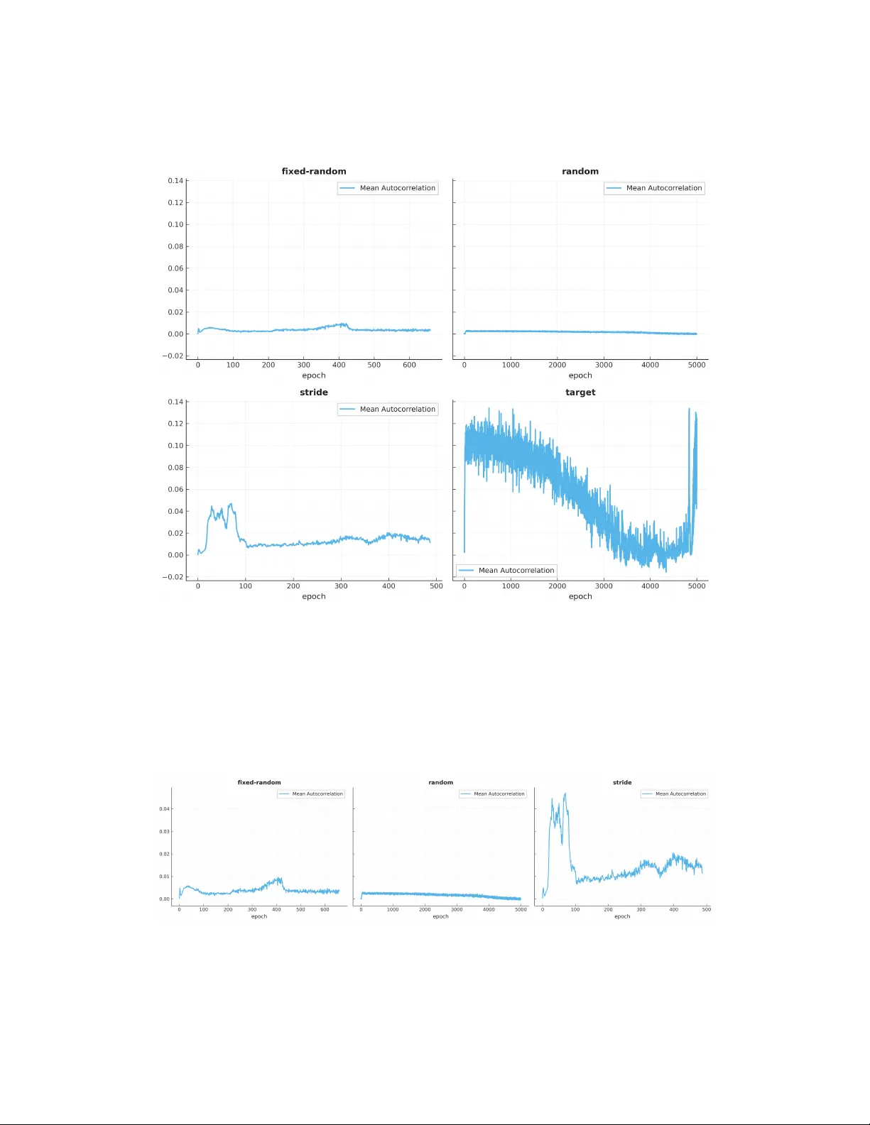
The Order Is The Message Jordan LeDoux Independent Researcher jordan.ledoux@gmail.com Abstract Neural network training under independent and identically distributed (IID) shuf- fling treats example ordering as a nuisance variable. W e show that it is an infor- mation channel. Counterfactual gradient decomposition rev eals that the ordering- dependent component accounts for approximately 85% of each epoch’ s cumulati ve gradient norm across all four ordering strategies tested, including IID shuffling. The channel is always acti ve; IID training ensures only that its contributions are incoherent, not that they are absent. The channel operates through Hessian-gradient entanglement between consecutiv e training steps: each parameter update displaces the model in a curved loss land- scape, modifying subsequent gradients in a direction determined by the ordering. Under IID shuffling or sampling, these ordering effects cancel over many steps; under consistent ordering, they constructi vely interfere, coherently dri ving feature acquisition. In a controlled experiment on modular arithmetic ( p = 9973 ), varying only exam- ple ordering while holding all else constant, two fix ed-ordering strategies achie v e 99.5% test accuracy by epochs 487 and 659 respecti v ely from a training set com- prising 0.3% of the input space, well belo w established sample complexity lo wer bounds for this task under IID ordering. The IID baseline achieves 0.30% after 5,000 epochs from identical data. An adv ersarially structured ordering suppresses learning entirely . The generalizing model reliably constructs a Fourier represen- tation whose fundamental frequenc y is the Fourier dual of the ordering structure, encoding information present in no indi vidual training e xample, with the same fundamental emerging across all seeds tested regardless of initialization or training set composition. W e discuss implications for training efficiency , the reinterpretation of grokking, and the safety risks of a channel that e vades all content-le v el auditing. 1 Introduction 1.1 Reading Guide This paper presents results across multiple levels of analysis. The following guide helps readers navig ate to the sections most relev ant to their interests, though the paper will make most sense if read in its entirety in the order presented. For headline results. Read Section 4.1.2 to understand the different models that were trained, Section 5.1.1 to understand ho w each model performed, and Section 5.1.2 to understand the e vidence of the model learning information that was only present in the order of the examples and not the examples themselv es. F or repr oduction. Read Section 4 to understand the experimental setup and how to access the code and data, and Section 5.1.1 to understand the nature of the results you will be looking for . Preprint. For theor etical explanation. Read Section 3 and 6.2 to understand the theoretical basis proposed and how the results confirm the predictions made from a theoretical basis. For safety and alignment discussion. Read Section 3 to understand the underlying basis of the claims, Section 5.1.2 to understand the evidence of ordering channel learning, and Section 6.7 for the safety and alignment concerns this work raises. 1.2 Motivation Large language models are trained on text corpora containing orders of magnitude more words than a human encounters in a lifetime. A frontier model may train on trillions of tokens, roughly three orders of magnitude more linguistic data than a typical child encounters in their first decade of life W arstadt and Bowman [2022]. Howe ver , humans routinely surpass these models in certain competencies after experiencing only a fraction of the data. Both humans and neural networks process natural language. Neural netw orks are demonstrably superior at statistical pattern extraction across large corpora: they can absorb and retain statistical regularities from billions of examples in ways that human memory cannot. The efficienc y gap therefore cannot be attributed to data quantity , nor straightforwardly to pattern recognition capability . Something provides a learning signal to humans that models, as currently trained, are not recei ving. Multi-modality of human learning is also unsatisfactory as a complete explanation, as man y of the tasks for which language models clearly underperform are strictly linguistic. While the multi-modal experience of humans no-doubt contributes to superior performance in some areas, it cannot on its own e xplain the entire discrepancy . The primary candidate is temporal structure. Human learning is profoundly non-IID. A child does not encounter sentences randomly sampled from the distrib ution of all language. A child hears a sentence about an object, then sees the object, then hears another sentence about it. Related concepts are encountered in temporal proximity . New ideas are presented in the context of pre viously established ideas. The sequential relationships between consecutiv e experiences carry information that no individual e xperience contains in isolation. Neural network training, by contrast, is designed to destro y this structure. The IID assumption that training examples should be shuffl ed or sampled into random order was imported from classical statistics, where it serv es as a mathematical con venience enabling tractable proofs of con ver gence and generalization bounds. It was adopted as standard practice in machine learning because it provides reliable, predictable training behavior: under IID sampling, the gradient at each step is an unbiased estimator of the true gradient of the content, and the mathematical machinery of stochastic optimization applies cleanly . Howe v er , the IID assumption was ne ver empirically demonstrated to be optimal for learning. It w as demonstrated to be sufficient , and in a field where the alternative w as poorly understood and difficult to control, sufficienc y was enough to establish it as uni versal practice. W e re visit this assumption. Recent w ork provides empirical grounds for doing so: Lu et al. Lu et al. [2022] demonstrated that deliberately optimizing the ordering of training e xamples, without changing the examples themselv es, produces prov ably and empirically faster con v ergence on tasks including CIF AR-10, W ikiT ext, and GLUE benchmarks. These results establish that ordering is not merely a nuisance variable, ho we ver both the mechanism through which ordering enters the gradient and the nature of the information it carries have remained uncharacterized. W e attempt to explain both of these. 1.3 Core Hypothesis W e propose that the sequential ordering of training examples constitutes an information channel that is distinct from the content signal within individual examples. The mechanism is straightforward: training is not a single operation but a sequence of gradient updates, and each update modifies the loss landscape on which subsequent updates operate. When consecutiv e examples produce gradients that are aligned with respect to a particular feature, the cumulativ e ef fect is a coherent directional signal to ward that feature’ s representation. When consecutiv e examples produce gradients that are randomly 2 oriented, these directional ef fects cancel ov er time, lea ving only the weaker signal contained in the statistical properties of individual e xamples. Under IID shuf fling, the ordering signal is randomized. Consecutive batches bear no systematic relationship to each other , so the inter-example gradient correlations point in random directions from step to step. Over suf ficient training, these random directional signals destructiv ely interfere and av erage to ward zero. What remains is the content signal: the information that can be extracted from the aggregate statistical properties of indi vidual e xamples, independent of their ordering. Under structured ordering, the ordering signal can be made coherent. If examples are sequenced such that consecutiv e batches produce gradients that are consistently aligned with respect to a target feature, the cumulativ e ef fect is a powerful, directed learning signal to ward that feature, a signal that operates on top of the content signal from the examples themselv es. Critically , this channel is not introduced by our method. It is always present in e very training run. IID shuffling does not eliminate it; it ensures that the channel carries noise rather than signal. Ev ery model ev er trained under IID conditions has been shaped by accidental ordering effects arising from the particular random shuffle used in that run. These effects are uncontrolled, unmeasured, and have been in visible to the field because IID guarantees their long-run cancellation. Our contribution is to identify this channel, demonstrate its strength, and show that it can be deliberately controlled. 1.4 Contributions This work makes the follo wing contrib utions: Empirical demonstration of the ordering channel. W e show that data ordering alone, with all other variables held constant including the exact set of training tokens, produces fundamentally dif ferent learned representations, training dynamics, and generalization outcomes. In our most controlled experiment, two fixed-ordering strategies achieve 99.5% test accurac y on a task where the IID baseline achiev es 0.30% from identical data and compute. Mechanistic characterization. W e provide a detailed mechanistic account of ho w the ordering signal operates, supported by comprehensi ve gradient decomposition, spectral analysis, and structural metrics collected at ev ery epoch. In the modular arithmetic setting, we trace the model’ s internal construction of a Fourier solution harmonic by harmonic, with each new frequency predictable in advance from the theory . Four -way directional control. W e demonstrate four ordering strategies applied to the same data: one that deliberately promotes a target feature ( S T R I D E ), one whose accidental structure is sufficient to dri ve generalization ( F I X E D - R A N D O M ), one whose strong but anti-coherent signal suppresses learning entirely (T A R G E T ), and one that is neutral (IID baseline, R A N D O M ). This four -way design isolates the ordering effect from all possible confounds we could account for and establishes that the channel provides controllable influence ov er feature acquisition, operating on a continuum determined by the interaction between the ordering signal’ s accumulated strength and its alignment with the task’ s representational requirements. Counterfactual gradient decomposition. W e introduce a measurement methodology that directly quantifies the ordering-dependent and ordering-independent components of the gradient at each training step, rev ealing that the ordering-dependent component accounts for the majority of gradient norm under all four ordering strategies. Identification of a covert training channel with safety implications. The ordering channel is in visible to all existing data auditing methods: ev ery indi vidual example is le gitimate, the aggregate data distribution is unchanged, and within-batch gradient statistics are indistinguishable between structured and random ordering. W e discuss the implications for AI safety oversight, particularly in settings where one model influences the training of another . Full repr oducibility . All code, training configurations, random seeds, collected metrics, and final model weights are published for immediate reproduction. The headline results can be v erified on a single GPU in under 36 hours; full reproduction with all instrumentation requires approximately 60 hours. 3 1.5 T erminology T o av oid ambiguity , we adopt the following terminology throughout this paper . Ordering channel. The information pathw ay through which the sequential arrangement of training examples influences learned representations. The channel is a property of gradient-based training itself, not of any particular ordering method. It is always acti v e; the question is whether it can carry productiv e, coherent signal, or if it can only act as regularizing noise. Ordering strategy . A method for determining the sequence in which training examples are presented. W e distinguish this from curriculum learning, which selects which examples the model sees; our ordering strategies determine only the sequence in which a fix ed set of examples is presented. All strategies see the same examples the same number of times. The four strategies used in our experiment (S T R I D E , F I X E D - R A N D O M , R A N D O M , and T A R G E T ) are described in Section 5. Content component and ordering component. The two components of the gradient identified by our counterf actual decomposition (Section 5.2). The content component is the portion of the observed gradient attrib utable to the data independent of presentation order . The ordering component is the residual: the portion that arises from the sequential structure of the epoch rather than from the statistical properties of indi vidual e xamples. The ordering component includes all ordering-dependent gradient information, productiv e or otherwise, and its magnitude characterizes the total gradient energy flo wing through the ordering channel at a gi ven point in training. Content signal and ordering signal. The productive subsets of the content and ordering components: the portions that result in lasting parameter changes which mov e the model toward competence at the task. The ordering signal is necessarily smaller than the ordering component, because the component includes ordering-dependent noise in addition to learnable information. Throughout this paper , we distinguish between the component (which is directly measurable via counterfactual decomposition) and the signal (which is inferred from its effects on learning outcomes such as spectral concentration and generalization). Entanglement term. 1 The Hessian-gradient interaction η H B ( θ ) · ∇ L A ( θ ) that arises when training on batch B after batch A has modified the parameters (described in Section 3.2). This is the mathematical object through which data ordering enters the gradient. W e use “entanglement” in its ordinary English sense of being intertwined: the term arises from the inseparable interaction between consecutiv e examples, not from either e xample alone. Constructive and destructi ve interference. When entanglement terms across consecutiv e training steps point in a consistent direction, they sum linearly ( constructive interference ) and the cumulati ve ordering signal gro ws proportionally with the number of steps. When they point in random directions, they sum as a random walk ( destructive interfer ence ) and the cumulati ve signal gro ws only as the square root of the number of steps. IID shuffling produces destructive interference; structured ordering can produce constructiv e interference along chosen directions. Critical learning period. The training window during which a particular feature’ s representation is forming and the ordering signal has maximal influence over its structure (Section 3). This is a per-feature property , not a global property of training: different features may ha v e critical learning periods at different points during optimization. 2 Related W ork Curriculum learning. Bengio et al. Bengio et al. [2009] demonstrated that ordering training examples from easy to difficult can impro ve conv ergence speed and generalization. Subsequent work has e xplored v arious difficulty metrics and scheduling strate gies Kumar et al. [2010], Grav es et al. [2017]. Our work dif fers fundamentally: curriculum learning v aries which examples the model sees and when, while our ordering strategies present the same e xamples in dif ferent sequences. The information channel we identify is carried by inter-e xample relationships, not by example selection. W u et al. W u et al. [2021] conducted thousands of ordering experiments and found that curricula ha ve 1 The analogy is apt: the term arises from the inseparable interaction between consecutiv e examples, not from either example alone. W e note that Cosson et al. Cosson et al. [2022] recently used this same phrase to describe spatial, overlapping gradient signals from different loss terms that cannot be disentangled. Howe ver , we retain our usage here, as we belie ve it is the most mechanically precise description of the temporal intertwining of parameter trajectories in a curved loss landscape. 4 only marginal benefits on clean data trained to conv ergence, attributing most benefits to dynamic dataset size. Their e xperiments used IID-shuffled orderings within each curriculum stage; our results suggest that it is fixed orderings, not curricula per se, that unlock the ordering channel, because IID shuffling within stages ensures the entanglement terms remain incoherent. Mohtashami et al. Mohtashami et al. [2022] showed that deterministic orderings can outperform random reshuffling, consistent with our finding that ordering consistency is a ke y v ariable. Grokking and delayed generalization. Po wer et al. Power et al. [2022] discov ered that models trained on algorithmic tasks exhibit sudden generalization long after memorizing the training set. Nanda et al. Nanda et al. [2023] provided mechanistic interpretability analysis showing that grokking in modular arithmetic in volv es the construction of Fourier features. Lee et al. Lee et al. [2024] introduced Grokfast, which accelerates grokking by amplifying slo w-varying gradient components. Our work pro vides a complementary perspectiv e: structured ordering eliminates the grokking delay entirely by coherently driving the model toward the F ourier solution from the first epoch, bypassing the memorization phase that produces the delayed generalization phenomenon. W e note that Mallinar et al. Mallinar et al. [2025] demonstrated grokking in non-neural k ernel machines (Recursi ve Feature Machines), which may operate outside the Hessian-gradient entanglement mechanism as described here. Whether the ordering channel contributes to grokking dynamics in non-SGD-trained models remains an open question. Non-IID training. The ef fects of non-IID data ordering ha ve been studied primarily as a problem to be mitigated, particularly in federated learning Zhao et al. [2018], Karimireddy et al. [2020]. Shumailov et al. Shumailov et al. [2021] demonstrated that adversarial data ordering alone—without modifying any training examples—can de grade or manipulate model behavior , establishing the secu- rity rele v ance of ordering ef fects. Bene v entano Bene ventano [2023] extended backward error analysis to SGD without replacement, showing that the Hessian-gradient interaction creates an ordering- specific implicit regularizer whose form depends on the permutation used. These works collecti vely demonstrate that non-IID ordering degrades con v ergence, reinforcing the field’ s commitment to IID shuffling. Ordering optimization. Lu et al. Lu et al. [2022] introduced GraB, which formulates example ordering as an online discrepancy minimization problem, using stale gradients from prior epochs to greedily construct permutations that provably con ver ge faster than random reshuf fling. GraB demonstrates practical gains on CIF AR-10, W ikiT e xt, and GLUE tasks, establishing that ordering optimization is beneficial be yond toy settings. Cooper et al. Cooper et al. [2023] extended this approach to distributed training, coordinating orderings across w orkers for prov ably accelerated con ver gence. These works treat ordering as a conv ergence-rate phenomenon: GraB minimizes gradient sum discrepancy to reduce the variance of the stochastic gradient estimator . Our frame work provides a complementary perspectiv e: in the entanglement framew ork, GraB’ s gradient balancing shapes the coherence of consecutiv e entanglement terms, and the conv ergence gains it achie ves are a specific consequence of making the ordering channel less noisy . Our contribution is to sho w that the channel can carry not only less noise but distinct, productiv e signal that the content channel does not provide, and to identify the mechanism through which this occurs. SGD ordering theory . The Hessian-gradient interaction through which ordering enters the gradient has been studied in the optimization literature. Smith et al. Smith et al. [2021] derived the same second- order cross-term via backward error analysis for SGD with random shuffling, showing it produces an ordering-dependent implicit regularizer . Barrett and Dherin Barrett and Dherin [2021] identified the analogous term for full-batch gradient descent. G ¨ urb ¨ uzbalaban et al. G ¨ urb ¨ uzbalaban et al. [2021] built their con v ergence analysis for random reshuf fling around controlling this Hessian-gradient term, and Recht and R ´ e Recht and R ´ e [2012] formalized ordering ef fects through non-commuting matrix products. More recently , HaoChen and Sra HaoChen and Sra [2019] and Ahn et al. Ahn et al. [2020] established tight con ver gence rates for SGD without replacement, and Mishchenko et al. Mishchenk o et al. [2020] pro vided simplified analyses with impro ved bounds. Rajput et al. Rajput et al. [2022] sho wed that the conv ergence gap between optimal and random permutations ranges from exponential to nonexistent depending on the function class, establishing that the potential benefit of ordering optimization is fundamentally problem-dependent. These works analyze the ordering-dependent term in service of con ver gence guarantees. Our contrib ution is to measure its magnitude empirically (showing it dominates per -step gradient norm), characterize its coher ence properties across ordering strategies, and demonstrate that it can be deliberately exploited as an information channel for feature acquisition. 5 Data influence and selection. Recent work on data attribution Koh and Liang [2017], Ilyas et al. [2022] and data selection for pretraining Xie et al. [2023], Engstrom et al. [2024] has studied ho w individual e xamples af fect model behavior . These approaches measure per -example influence on the trained model; our work identifies an orthogonal axis of influence that arises from the r elationships between consecutiv e examples rather than from an y example indi vidually . Fourier featur es in neural networks. The emergence of Fourier features in networks trained on modular arithmetic is well-established Nanda et al. [2023], Zhong et al. [2023], Gromov [2023]. Gromov Gromo v [2023] provided analytical solutions for the optimal F ourier representations. Our contribution is sho wing that structured ordering controls whic h Fourier features emer ge and at what rate, with the fundamental frequency determined by the number -theoretic properties of the ordering structure. 3 Theoretical Framew ork This section presents a mechanistic account of how data ordering produces a learning signal. W e begin from the well-kno wn T aylor expansion of the gradient at consecuti ve training steps Smith et al. [2021], Barrett and Dherin [2021], identify the specific term through which ordering exerts its influence, reinterpret it as an information channel with measurable coherence properties, and connect the theoretical predictions to the empirical measurements reported in Section 5. 3.1 Non-Commutativity of SGD Updates It is well kno wn that SGD updates do not commute in non-con vex landscapes Bottou et al. [2018]: training on batch A then B yields a different parameter state than B then A , because each update shifts the point at which the next gradient is e v aluated. Under conv exity this is irrele v ant to the final solution; under the non-con v ex losses of neural netw orks, it means the training trajectory , and thus the basin of con ver gence, depends on ordering. A substantial body of work has quantified ho w permutation order af fects con vergence rates Safran and Shamir [2020], G ¨ urb ¨ uzbalaban et al. [2021], HaoChen and Sra [2019], Ahn et al. [2020], Mishchenko et al. [2020], and backward error analysis has shown that the Hessian-gradient cross-term arising from finite learning rates produces an ordering-dependent implicit regularizer Smith et al. [2021], Barrett and Dherin [2021]. Bene v entano Benev entano [2023] extended this analysis to SGD without replacement, showing that the resulting regularizer is permutation-specific : different orderings of the same data produce dif ferent implicit regularizers, meaning the choice of permutation shapes the optimization landscape itself. Recht and R ´ e Recht and R ´ e [2012] formalized the non-commutati vity through products of non-commuting operators. These analyses focus on con ver gence speed to a fixed optimum and on the regularization properties of the cross-term. That the term can be practically exploited has been demonstrated by Lu et al. Lu et al. [2022], whose GraB algorithm optimizes data permutations by minimizing gradient discrepancy and achieves measurable con ver gence gains on standard benchmarks. What has been missing is a characterization of this term as an information channel : an empirical decomposition that measures how much of each gradient step is attributable to ordering, how the coherence of this component varies across ordering strategies, and whether the channel can be deliberately exploited to control which features a model acquires. W e provide this next. 3.2 The Ordering Signal: A Hessian-Gradient Interaction 3.2.1 Derivation Consider two consecuti ve training steps. At parameters θ , we update on batch A : θ ′ = θ − η ∇ L A ( θ ) W e then compute the gradient for batch B at the new parameters θ ′ . Expanding this gradient to first order around θ : ∇ L B ( θ ′ ) ≈ ∇ L B ( θ ) + H B ( θ ) · ( θ ′ − θ ) 6 where H B ( θ ) = ∇ 2 L B ( θ ) is the Hessian of the loss for batch B ev aluated at θ . Substituting the update rule: ∇ L B ( θ ′ ) ≈ ∇ L B ( θ ) | {z } content term − η H B ( θ ) · ∇ L A ( θ ) | {z } entanglement term (1) The gradient used for the second update thus has two components: The content term , ∇ L B ( θ ) : the gradient that batch B would produce if A had not been trained on first. This is the standard gradient signal; it depends only on the content of B and the current parameters. The entanglement term , − η H B ( θ ) · ∇ L A ( θ ) : an additional gradient contribution arising from the interaction between batch A ’ s gradient and batch B ’ s loss curvature. This term depends on the r elationship between A and B , specifically on how the direction of A ’ s update aligns with the curvature structure of B ’ s loss. This decomposition is standard; the same Hessian-gradient cross-term appears in analyses of implicit regularization in SGD Smith et al. [2021], Barrett and Dherin [2021] and in con ver gence proofs for random reshuffling G ¨ urb ¨ uzbalaban et al. [2021], HaoChen and Sra [2019]. What has not been appreciated is that this term constitutes an information channel . The entanglement term does not exist in an y indi vidual example; it arises only from the sequential interaction between consecutiv e examples. It is the mathematical object through which data ordering exerts its influence on learning, and its coherence properties, (whether it constructively or destructiv ely interferes across steps), determine whether the channel carries usable signal or self-canceling noise. 3.2.2 Behavior Under Random Ordering Under IID shuf fling, the gradient ∇ L A ( θ ) is drawn from a distribution that is independent of B . The entanglement term H B ( θ ) · ∇ L A ( θ ) therefore projects a random direction through B ’ s Hessian. Over man y steps, these projections point in random directions and their cumulati ve effect a v erages tow ard zero. This is the cancellation that underpins classical conv ergence guarantees for SGD with random reshuffling G ¨ urb ¨ uzbalaban et al. [2021], Mishchenko et al. [2020]. The cancellation is statistical, not exact. In any finite training window , the random entanglement terms do not perfectly cancel; there is always some residual ordering effect. This residual is an uncontrolled source of variance between training runs that is typically attributed to “initialization noise” or “training stochasticity . ” Our framework suggests that a portion of this variance is attrib utable to accidental ordering effects that persist through finite-sample noise in the cancellation. In expectation, IID shuf fling ensures that the entanglement terms cancel cumulati v ely , so the long-run parameter trajectory is driv en by the content term alone. At each individual step, howe ver , the entanglement term remains large: our measurements show it accounts for the majority of per -step gradient norm ev en under IID conditions (Section 5.2). This is the re gime that classical con ver gence theory describes. 3.2.3 Behavior Under Structur ed Ordering Under structured ordering, the relationship between consecutive batches is no longer random. If batches A and B are selected such that ∇ L A ( θ ) aligns with a principal eigen vector of H B ( θ ) , the entanglement term is amplified: B ’ s curvature structure reinforces A ’ s gradient direction, producing a large, coherent contrib ution to the ef fectiv e gradient. More precisely , let H B = P i λ i v i v T i be the eigendecomposition of the Hessian. Then: H B · ∇ L A = X i λ i ( v T i ∇ L A ) v i (2) The entanglement term is largest when ∇ L A is aligned with eigen vectors corresponding to large eigen v alues λ i , that is, when A ’ s gradient points along directions of high curvature in B ’ s loss. Structured ordering exploits this by selecting consecutiv e examples whose gradients are mutually aligned and point along high-curvature directions of each other’ s loss surfaces. Importantly , the entanglement term need not dominate the entire gradient to have a significant impact on learning. It is suf ficient for it to operate on the subset of parameters that control the feature being 7 acquired, for instance the embedding weights that encode a particular Fourier frequency . A coherent signal in this subspace can guide the corresponding feature into a particular basin of attraction, after which the remaining parameters adjust to accommodate the committed representation through ordinary gradient descent on the content signal. 3.2.4 Signal Strength The relati v e magnitude of the entanglement term v ersus the content term depends on three factors: the learning rate η (which scales the displacement and thus the entanglement term linearly), the spectral norm of the Hessian (which determines how strongly curv ature amplifies the displacement), and the alignment between consecutive gradients (which determines what fraction of the displacement is amplified). For neural networks in typical training regimes, the Hessian has a small number of large eigen values and a large number of small ones, a well-documented spectral structure. When consecutiv e gradients are aligned with the lar ge-eigen v alue directions, the entanglement term can be comparable to or larger than the content term. Our per -step Hessian measurements (Section 5.4, Appendix A.3) reveal that the entanglement and content terms are in fact nearly identical in both magnitude and direction (cosine similarity > 0 . 999 ), making the observed gradient a small residual of two large, nearly-canceling vectors. The ordering signal liv es in this residual: small angular differences between entanglement and content, determined by which batch follo ws which, are amplified into large directional changes in the gradient the optimizer sees. Our epoch-lev el counterfactual decomposition (Section 5.2) confirms that this per -step structure accumulates: the ordering component accounts for the majority of each epoch’ s cumulative gradient norm. Component vs. signal. It is important to note that the ordering component contains all ordering- dependent gradients, not only the producti ve ones. Even under highly structured ordering strategies, the component will contain noise in addition to learnable signal. The magnitude of the ordering component relativ e to the content component characterizes the channel’ s bandwidth, not the amount of productiv e learning that occurs through the ordering channel. 3.2.5 Extension to Adaptive Optimizers The deriv ation abov e uses vanilla SGD for clarity , but the mechanism is not specific to SGD. The entanglement term arises from the non-commutati vity of parameter updates in curv ed loss landscapes, and any optimizer that produces a parameter displacement creates a Hessian-displacement interaction with the subsequent batch. In the general case, let ∆ θ denote the actual parameter displacement produced by an optimizer step on batch A . The T aylor expansion of the subsequent gradient becomes: ∇ L B ( θ + ∆ θ ) ≈ ∇ L B ( θ ) + H B ( θ ) · ∆ θ (3) Under SGD, ∆ θ = − η ∇ L A ( θ ) and the entanglement term reduces to Equation 1. Under Adam Kingma and Ba [2015] or AdamW Loshchilov and Hutter [2019], the displacement is: ∆ θ = − η ˆ m t √ ˆ v t + ϵ (4) where ˆ m t and ˆ v t are the bias-corrected first and second moment estimates. This transformation modulates the ordering channel through three pathways. Amplified displacement. Adam’ s per -parameter adaptiv e scaling can produce displacements whose norm substantially exceeds the raw gradient norm, particularly for parameters with small but consistent gradients. Because the entanglement term scales with ∥ H B · ∆ θ ∥ , larger displacements produce proportionally larger entanglement, amplifying the ordering channel relati ve to the SGD baseline. Momentum as temporal integration. The first moment ˆ m t is an exponential moving average of past gradients with decay rate β 1 . Under structured ordering, if consecutiv e gradients share a consistent component in some subspace (the ordering signal), momentum accumulates this component across steps. Under IID ordering, the ordering components of consecutiv e gradients point in unrelated 8 directions and partially cancel within the momentum buffer . Momentum therefore acts as a temporal integrator that preferentially preserves coherent signals, whether from content or from ordering, while attenuating incoherent ones. The displacement ∆ θ inherits this filtered signal, and the entanglement term on the next step reflects the accumulated, filtered history rather than only the most recent batch. Selective parameter scaling. The second moment ˆ v t normalizes each parameter by its recent gradient variance. Parameters that receiv e consistent gradient signals (low variance) are assigned larger ef fectiv e learning rates; parameters that receiv e noisy signals (high variance) are assigned smaller ones. Under structured ordering, the gradient signal is more consistent along parameters that participate in the feature being dri ven by the ordering, producing lar ger ef fectiv e learning rates for precisely those parameters. This creates a feedback loop: the ordering signal is selectively amplified in the subspace it targets. The interaction between these pathways can be complex. Momentum smoothing and adaptive scaling can either amplify or attenuate the ordering signal depending on the relationship between the ordering’ s temporal coherence and the optimizer’ s characteristic timescales ( 1 / (1 − β 1 ) for momentum, 1 / (1 − β 2 ) for v ariance estimation). A full analytical treatment of these interactions is beyond the scope of this work. What matters for the present argument is that the Hessian-displacement mechanism persists under any optimizer that produces non-zero parameter updates, and that adaptive optimizers introduce additional structure into the displacement v ector that can dif ferentially modulate the ordering channel’ s strength across parameter subspaces. W e v erify this empirically in Section 5.4. 3.3 Constructive and Destructi ve Interference The wa ve-interference analogy is more than a metaphor . The entanglement terms from consecutive training steps are additi ve contrib utions to the ef fectiv e gradient. When these contributions point in a consistent direction across many steps, they sum constructi vely: the cumulative ordering signal grows linearly with the number of steps. When they point in random directions, they sum lik e a random walk: the cumulative signal gro ws only as the square root of the number of steps, and the signal-to-noise ratio decreases with training duration. This framing explains se veral empirical observ ations: Why IID training e ventually works mechanistically . Even under random ordering, the content term is present at e very step and points in a consistent direction (to ward reducing the training loss). The ordering noise slo ws con v ergence and may misdirect the optimization into suboptimal basins, but it does not prevent con ver gence entirely: the content signal e ventually dominates the random ordering noise giv en suf ficient training. Why structured ordering is dramatically more efficient. Under structured ordering, both the content term and the entanglement term are aligned within some critical subspace of the feature. The model receiv es a coherent signal from two channels simultaneously rather than one. Why anti-coherent ordering is destructive. If the ordering produces entanglement terms that ov erwhelm the content signal but whose structure is anti-aligned with useful feature acquisition, the model is dri ven to ward de generate representations. The ordering signal does not merely add noise; it coherently organizes specific components of the model while preventing others from forming, because consecutiv e batches produce gradients that are structured but self-contradictory with respect to the task. This is distinct from the incoherent case ( R A N D O M ), where the ordering signal cancels ov er time. Under anti-coherent ordering, the signal does not cancel; it accumulates tow ard a basin that is organized but not useful. This is the failure mode we observ e with the T A R G E T ordering strategy (Section 5), and it is the failure mode that historically led researchers to conclude that non-IID ordering is harmful. Why the ordering signal is in visible to standard monitoring. The entanglement term modifies the gradient for batch B based on what happened during batch A . W ithin any single batch, the gradient statistics appear normal: the ordering signal manifests as temporal correlations acr oss batches, not as anomalies within a batch. Standard training monitoring examines per -batch metrics but does not examine cross-step gradient correlations. The ordering channel operates in a dimension that existing monitoring tools do not measure. 9 Additionally , the ordering component of the gradient norm is large under all ordering strate gies (Section 5.2): the counterfactual decomposition shows that ordering accounts for the majority of each epoch’ s cumulativ e gradient magnitude ev en under IID shuffling. Because its cancellation tow ard zero is a long-horizon statistical ef fect, any short windo w of training will e xhibit substantial ordering-induced gradient structure regardless of whether the ordering is deliberate, productiv e, or impactful to the o verall training. Distinguishing a coherent signal embedded in the ordering component from the large but incoherent background present in e very training run requires kno wing which directions in parameter space to monitor , which in turn requires prior knowledge of the tar get behavior . W ithout this, the signal may be indistinguishable from the noise floor . 3.4 Basin Selection and the Critical Learning P eriod In non-con ve x optimization, the loss landscape contains many basins of attraction, parameter regions that produce locally minimal loss. Dif ferent basins may achiev e similar training loss but correspond to qualitativ ely dif ferent learned representations. The ordering signal influences which basin the optimization trajectory enters. Because the entan- glement term is most influential when the loss landscape is highly curved with respect to a forming feature, when the model’ s representation of that feature is still undif ferentiated and small perturbations can determine its structure, the ordering during this period can determine the basin for that feature’ s representation. W e term this the critical learning period for a feature. In our experiment, where the model learns a single representation, the critical learning period coincides with early training: the S T R I D E model identifies the fundamental frequency F = 101 within the first 3 epochs, and by epoch 30 the spectral structure of the e v entual solution is already visible. Howe ver , we expect the critical learning period to be a per-feature property in general, not a global property of training. A feature that begins forming midway through training would hav e its critical learning period at that point, not at initialization. The ordering signal’ s influence on that feature would be maximal during its period of formation, regardless of when during o verall training that occurs. If the ordering signal’ s influence is concentrated during feature formation, this should be observ able in the ordering fraction at the layers most inv olved in the emerging representation. As the model commits to a basin and the relev ant parameters leav e the region of high curv ature, the same ordering should produce diminishing gradient displacement in those parameters, not because the external signal has weak ened, but because the parameters ha ve mov ed to a region where it no longer has le verage. The ordering fraction at specific layers should therefore decline as the corresponding feature crystallizes, with the rate of decline tracking the pace of feature formation. W e observe this ef fect in Section 5.2. This distinction has practical implications. If the critical learning period were global and early , one could in principle audit the ordering only at the st art of training. If it is per-feature and distrib uted throughout training, the window of vulnerability to ordering-based influence is coe xtensiv e with training itself. 3.5 Empirical Predictions The theoretical framew ork generates se veral empirically testable predictions: 1. The ordering component of the gradient should be measurable by comparing the gradient under structured ordering to the gradient under counterfactual random ordering of the same examples. 2. The ordering signal should produce measurable spectral concentration in the model’ s weight representations. 3. Ordering that is both strong and misaligned with the task’ s representational requirements should prev ent con v ergence. 4. The ordering signal should be strongest early in feature formation, when the loss landscape is most curved. 5. The ordering and content components should be partially but not fully aligned, indicating the ordering channel carries partially independent information. 10 6. Under an adapti ve optimizer , the displacement amplification and selectiv e scaling should produce entanglement energies substantially e xceeding the SGD prediction, with the amplifi- cation varying across parameter subspaces according to each subspace’ s gradient consistenc y . These predictions are confirmed by the experimental results presented in Section 5. 4 Methodology 4.1 Experimental Setup 4.1.1 T ask and Motiv ation W e study addition modulo a prime p = 9973 . The task is to learn the function f ( a, b ) = ( a + b ) mo d p from a sparse subset of the input space. This setting is chosen for three reasons: (1) the problem has known analytical solutions in terms of Fourier features Nanda et al. [2023], Gromov [2023], enabling mechanistic verification of learned representations; (2) the problem is simple enough that all relev ant metrics can be computed at ev ery epoch within a tractable time budget; and (3) the grokking phenomenon in this setting is well-studied, providing a rich baseline of prior results against which our ordering effects can be measured. Preliminary experiments at p = 97 showed rapid generalization across S T R I D E , F I X E D - R A N D O M , and R A N D O M strategies under high data density , consistent with the content signal being sufficient in that re gime. The choice of p = 9973 at 0.3% data density was designed to place the e xperiment belo w the theoretical critical data fraction for IID ordering, isolating the ordering channel’ s contribution in a regime where content alone is provably insuf ficient. The large prime additionally provides finer spectral resolution (9,973 possible frequencies versus 97), enabling detailed tracking of harmonic emergence and clear spectral dif ferentiation between ordering strategies. At p = 97 with 26.5% data density , all three non-adversarial strategies generalize, with fixed orderings achieving approximately 20% faster con vergence than IID shuffling (single seed). The ordering channel’ s contribution is modest in this regime because the content signal alone is sufficient for generalization. This contrasts with the p = 9973 experiment at 0.3% density , where the content signal is insuf ficient and the ordering channel determines whether generalization occurs at all. The ordering channel’ s practical importance thus scales inv ersely with content signal adequacy . This aspect is discussed in greater depth in Section 6.4. 4.1.2 Models and T raining Architectur e. W e use a two-layer pre-LayerNorm transformer with embedding dimension 256, 4 attention heads, and feedforward dimension 2048 (the PyT orch nn.TransformerEncoderLayer default). Each integer a ∈ { 0 , . . . , p − 1 } is embedded via a learned embedding table and summed with a learned positional embedding indicating operand position. The model processes pairs ( a, b ) , mean-pools over the sequence dimension, and produces a probability distribution over outputs c ∈ { 0 , . . . , p − 1 } via a linear decoder . T raining data. W e sample 300,000 input pairs ( a, b ) uniformly at random as the training set, comprising approximately 0.3% of the 9973 2 ≈ 10 8 possible pairs. A separate test set of 1,000,000 pairs is sampled from the remaining pairs. The same training and test sets are used across all ordering strategies. Optimizer . AdamW with weight decay 0 . 1 , and default momentum parameters ( β 1 = 0 . 9 , β 2 = 0 . 999 ). Scheduler . Learning rate follows a cosine annealing schedule over 5,000 epochs with learning rate 1 × 10 − 3 , and minimum learning rate 5 × 10 − 7 . T raining regime. Batch size is 256. All models are trained for 5,000 epochs, or until they score greater than or equal to 99.5% on the test set. 11 Ordering strategies. W e compare four strategies: • S T R I D E : Examples are sorted by ( a mo d s, a ) where s = ⌊ √ p ⌋ = 99 . This creates a strided traversal of the input space that groups nearby elements within blocks of size 99. The ordering is computed once and held fixed across all epochs. • F I X E D - R A N D O M : A single random permutation is generated at initialization (determined by the random seed) and held fixed across all epochs. This permutation will necessarily hav e some cyclic structures that are useful for F ourier features, but those structures will be noisy and undesigned. • R A N D O M : Standard IID shuf fling with a fresh random permutation each epoch. • T A R G E T : Examples are sorted directly by their output value ( a + b ) mo d p . This creates maximum structure, with consecuti ve e xamples having consecutiv e outputs, producing an ordering signal that is both strong and self-contradictory , a combination that prev ents stable learning. Shared conditions. All four models share the same architecture, parameter initialization (via a shared random seed), training set, optimizer, hyperparameters, and compute budget. The only variable is the ordering of training examples within each epoch. 4.2 Reproducibility and Data 4.2.1 Reproduction Steps The code that was used to produce the results in this paper can be found at: github .com/JordanRL/OrderedLearning Clone the repository and then checkout the tag ’paper-data-v3’, which is the tag that was used to generate the exact data found in this paper . The raw data collected, including weights, ra w metrics, and checkpoints, can be found at: github .com/JordanRL/ExperimentOneData This raw data includes an experiment config.json file for each strategy that contains the recorded en vironment information of the environment that generated the data. It was run on RunPod cloud computing resources, using an R TX 4090 pod. It ran in a template that was generated from the Dockerfile which is contained in the code repository . The e xact commands used, and the exact sequence they were used in, are e xplained in the README.md of the repository . The code is written to generalize to other experiments, and is released under an MIT license. The code contains all of the metric collection processes, and also contains details on ho w another researcher could add their own additional metrics if so desired. The author is av ailable to other researchers who wish to utilize the framew ork for their o wn experi- ments to answer questions and provide limited support as time allo ws. 4.2.2 Deterministic Behavior The framew ork supports deterministic, bit-for-bit reproduction of machine learning experiments out of the box, and guarantees that different strategies within the same e xperiment will receiv e the same initialization. This includes isolation of the code that is e xecuted to compute and collect metrics. The framew ork clones the entire training state, including the model, optimizer , and RNG state, prior to ev ery point where instrumentation is run, then automatically restores that state prior to the training loop resuming. This ensures that any type of instrumentation could be added without affecting the deterministic behavior of the frame work. Reproduction with the same e xact en vironment should result in bit-for-bit identical results. Repro- duction with different en vironments, such as different hardware, should result in statistically similar results, but dif ferent e xact data. 12 4.2.3 Seed Sensitivity Sweeping All four strategies were trained with seed 199 for the instrumented runs presented in this paper . This seed was selected based on preliminary S T R I D E runs as approximately median in generalization time. T o assess seed sensiti vity , non-instrumented runs observing only test accuracy were conducted for S T R I D E and F I X E D - R A N D O M across seeds 31, 42, 199, 242, 555, and 9973. For S T R I D E , fiv e of six seeds generalized within 700 epochs; seed 555 did not fully generalize within this b udget, reaching approximately 20–25% test accuracy before stalling. Notably , F = 101 emerged as the peak embedding frequency on e very seed tested, including seed 555 and despite each seed selecting a different random subset of 300,000 training pairs. Seed 555’ s failure was not in identifying the fundamental; it was in extending the harmonic series beyond the first fe w frequencies, suggesting that the initialization geometry at this seed was unfa vorable for completing the F ourier construction rather than for beginning it. For F I X E D - R A N D O M , all six seeds generalized within 700 epochs. The R A N D O M and T A R G E T strategies were not tested across additional seeds, as their outcomes (memorization without generalization and failure to learn, respecti vely) are consistent with established results for IID and adversarial ordering in this domain Po wer et al. [2022], Shumailo v et al. [2021]. Additionally , as this work was self-funded, there was a question of where the av ailable resources would be best spent. 4.2.4 Instrumentation and Metrics T o properly interpret and understand the results presented in this paper , we utilize a variety of instrumentation and metrics. While some of these are commonly used in both research and industry , other techniques we’ ve emplo yed bear further explanation. A full accounting of all collected metrics are av ailable in Appendix B.1. Counterfactual Decomposition. T o generate this metric, we checkpoint the model and run K=3 independently shuffled epochs from the same parameter state. The mean gradient across these shuffled runs approximates the order-independent gradient. The content component is extracted by projecting the observ ed gradient onto the calculated order -independent gradient. The ordering component is defined as the residual between the gradient from the actual ordered epoch and this content component, isolating the contribution of sequential structure to the training signal. For further details, see Appendix A.1. Gradient Projection to Solution. T o assess whether training dynamics mo ve the model to ward its final con v erged state, we compute the cosine similarity between the ne gated gradient −∇ L (the descent direction) and the displacement v ector θ ref − θ current , where θ ref is the fully trained model’ s pa- rameters. A positive v alue indicates the gradient points to ward the solution; a ne gati ve v alue indicates the optimizer must navigate around regions of high curvature rather than proceeding directly . W e apply this projection both to the full gradient and to the ordering and content components separately , enabling direct comparison of which component is more solution-aligned. See Appendix A.2 for interpretation cav eats. Hessian Entanglement Measurement. The entanglement term η H B · ∇ L A —the mechanism by which batch ordering enters the gradient (Section 3)—can be measured directly at each training step via finite-dif ference Hessian-vector products. W e capture the pre vious batch’ s gradient before it is cleared, then compute the Hessian-vector product after the subsequent forward-backw ard pass. This yields per-step estimates of the entanglement norm, its fraction of the observ ed gradient energy , and its directional coherence across consecuti ve steps. See Appendix A.3 for the full procedure and deriv ed metrics. 13 Figure 1: The S T R I D E and F I X E D - R A N D O M strategies generalize quickly; the R A N D O M strategy memorizes but is unable to generalize within the compute budget; the T A R G E T strategy fails to either generalize or memorize, nev er improving be yond chance-le vel performance. 5 Experimental Results 5.1 Results 5.1.1 Generalization The four ordering strate gies produce qualitati vely dif ferent generalization outcomes from identical data and compute. The S T R I D E model achie ves 99.5% test accuracy by epoch 487. T rain accuracy rises rapidly , reaching 90% by approximately epoch 140, while test accuracy remains below 5% until approximately epoch 200 before accelerating sharply . The peak train-test gap of approximately 90% occurs around epoch 160. Despite this gap, the model is b uilding the generalizing representation from the earliest epochs: by epoch 3, the peak frequenc y in the embedding weight spectrum is F = 101 , the fundamental of the final generalizing solution (Section 5.1.2). The mechanistic significance of this gap is discussed below . The F I X E D - R A N D O M model achie ves 99.5% test accurac y by epoch 659, follo wing a similar trajectory: rapid train accuracy growth, a delayed test accuracy takeoff (peak train-test gap of approximately 83% around epoch 220), and an acceleration phase that brings both to con ver gence. Like S T R I D E , the model orients toward its generalizing Fourier representation within the first ten epochs, with the peak embedding frequency locking to F = 2205 by epoch 7. This result is striking: the F I X E D - R A N D O M ordering contains no task-specific structure whatsoever . It is a random permutation held constant across epochs. The role of structure is discussed in Section 5.1.5. 14 The R A N D O M model achieves 0.30% test accuracy after 5,000 epochs. This is above the chance- lev el performance of 0.01% for p = 9973 , howe v er the model does not display characteristics of generalization. It memorizes the training set completely but does not generalize within the training budget. This is the standard grokking regime: under IID ordering, generalization on modular arithmetic requires thousands of additional epochs beyond memorization. The T A R G E T model fails to achiev e meaningful train or test accuracy . The ordering signal is both strong and anti-aligned with the task’ s representational requirements, destabilizing optimization as predicted by the dose-productivity frame w ork of Section 3. See Section 5.1.4 for analysis. The train-test gap under structured ordering . The train-test gap in the fixed-ordering strategies might appear similar to the memorization phase observed in standard grokking, b ut the underlying mechanism is dif ferent. In standard grokking, the model first constructs a memorization table and then gradually replaces it with a generalizing circuit Nanda et al. [2023]. Under S T R I D E and F I X E D - R A N D O M , the spectral evidence sho ws that the model is constructing the generalizing representation from the start. The peak embedding frequency locks to the solution’ s fundamental within the first few epochs, and subsequent harmonics emerge sequentially as training progresses (Figure 2). What the models lack during the g ap period is not the correct representation but suf ficient spectral resolution: a small number of harmonics can fit the sparse training points (which occupy only 0.3% of the input space) while remaining too coarse to interpolate correctly across the full cyclic group. Each subsequent harmonic refines this resolution, and test accuracy rises in lockstep. The train-test gap therefore reflects an underdetermined F ourier interpolation, not a memorization table being gradually replaced by a generalizing circuit. The model is building tow ard a Fourier solution of the kind characterized analytically by Gromov Gromov [2023], b ut has not yet accumulated enough harmonics to resolve the full c yclic group. 5.1.2 Spectral Analysis Figure 2: Both the S T R I D E and F I X E D - R A N D O M strategies accumulate frequency power early in training, and both end training with a similar amount of power concentrated in significant frequencies. The S T R I D E strategy or ganizes much earlier than the F I X E D - R A N D O M strategy , but the F I X E D - R A N D O M achiev e a higher peak concentration of frequency po wer . Gromov Gromo v [2023] sho wed that modular arithmetic can be solv ed by F ourier representations ov er the cyclic group, and provided analytical e xpressions for network weights that achiev e 100% accuracy . F ourier analysis of the S T R I D E model’ s embedding weights rev eals that it constructs such a representation, but rooted in a harmonic series whose fundamental frequency F = 101 is determined by the ordering rather than by the task alone. This frequency is the Fourier dual of the sort stride s = 99 ov er the cyclic group Z 9973 . The precise relationship is F = ⌊ p/s ⌉ = ⌊ 9973 / 99 ⌉ = 101 , which corresponds to the natural sampling frequency of the stride pattern in the Fourier domain. This relationship between the stride value s and the fundamental frequency F was confirmed as described in Appendix B.2. 15 The harmonic series follows a doubling pattern with Nyquist folding at p/ 2 = 4986 . 5 : 101 , 202 , 404 , 808 , 1616 , 3232 , 6464 → 3509 , . . . where 6464 mo d 9973 = 6464 folds to 9973 − 6464 = 3509 upon exceeding the Nyquist frequenc y . By the final epoch, 40 frequencies achieve po wer more than 10 × abov e uniform baseline, and the 14 highest-power frequencies are all predicted harmonics of F = 101 . Frequency F = 101 becomes the peak frequency in the embedding spectrum by epoch 3 and crosses the 10 × significance threshold by epoch 14. Subsequent harmonics emerge sequentially: F = 202 at epoch 21, F = 404 at epoch 39, F = 808 at epoch 61, and so on at roughly re gular intervals (Figure 2). This sequential harmonic construction is visible in the significant frequency po wer plot, which shows the stack ed po wer of all significant frequencies across training. The F I X E D - R A N D O M model exhibits the same qualitative pattern with dif ferent frequencies. Its peak embedding frequency locks to F = 2205 by epoch 7, the initial spectral dominant of its particular random permutation, and subsequent frequencies emerge sequentially from there. By the final epoch, 39 frequencies exceed the 10 × significance threshold, with F = 3234 having surpassed F = 2205 as the highest-power frequenc y . Critically , the frequencies that emerge bear no relationship to the stride harmonic series; instead, they reflect the spectral structure of the specific random permutation used. The model e xtracts whate ver periodic structure exists in its fixed ordering and constructs the corresponding Fourier basis, with the relativ e power of dif ferent frequencies shifting as the representation matures. 5.1.3 Spectral Entropy Figure 3: The Embedding Spectral Entropy (blue), Decoder Spectral Entropy (orange), and Neuron Spectral Entropy (green) for all four strategies. This measures the amount of uniformity in weight distrib utions, with 1.0 being perfectly uniform, and 0.0 being maximally concentrated. 16 W e track spectral entropy across three levels: the embedding weight matrix, the decoder weight matrix, and per-neuron within the embedding. For a normalized power spectrum P = { P k } ov er frequencies k , spectral entropy is defined as S = H ( P ) log p = − P k P k log P k log p where p is the prime modulus. This normalization ensures S ∈ [0 , 1] : S = 1 when po wer is uniformly distributed across all frequencies, and S → 0 when power is concentrated on a single frequenc y . Figure 3 shows all three measures for each strate gy . In the generalizing strategies, all three entropy measures decline together . The S T R I D E model’ s embedding spectral entropy declines from near 1.0 to approximately 0.60, with a minimum of 0.60 during the most acti v e phase of harmonic construction. The decoder and neuron-level entropies follow similar trajectories, with neuron-le vel entrop y declining fastest, reaching approximately 0.40 before recov ering. The F I X E D - R A N D O M model shows a nearly identical pattern with slightly deeper minima: embedding to 0.58, neuron-lev el to 0.42. That neuron-level concentration leads aggregate concentration suggests spectral organization begins at the level of indi vidual neurons before becoming visible in the full embedding spectrum. The R A N D O M model shows almost no spectral concentration at an y le vel. All three entropy measures remain almost flat near their initialization values throughout 5,000 epochs. The T A R G E T model shows a striking dissociation between components. The decoder spectral entropy drops rapidly and remains low throughout training, indicating strong spectral organization in the output layer . The embedding, by contrast, remains near 1.0 for the first 4,000 epochs before a sharp late-training decline. The ordering signal organizes the output layer while the input layer fails to form usable representations until a late collapse dri ven by weight decay . This dissociation is analyzed further in Section 5.1.4. 5.1.4 The T A R G E T Failur e Mode The T A R G E T model confirms the dose-productivity prediction from Section 3. After 5,000 epochs, T A R G E T achieves 0.02% train and 0.01% test accurac y , at chance level ( 1 /p = 0 . 01% ). Its loss f alls to 7.36 by epoch 5,000, below the initialization value of 9.22 ( ≈ ln p , maximum entropy over the output space), indicating some internal reorganization despite chance-le v el accuracy . But the model does not generalize. The ordering fraction of gradient norm av erages 89%, compared to 87% for R A N D O M , and the cosine similarity between consecuti v e epoch gradients spans − 0 . 97 to +0 . 96 (versus − 0 . 21 to +0 . 50 under R A N D O M ), with approximately 70% of pairs anti-correlated. The ordering channel is po werfully activ e, but because T A R G E T sorts by output value, each batch spans only ∼ 8 –9 consecutiv e output classes and the target distrib ution shifts completely between adjacent batches, producing a self-contradictory signal. Despite this failure, T A R G E T dri ves the most dramatic spectral reorganization of any strategy , but only in the decoder . The decoder’ s spectral entropy drops from 0.62 after the first epoch to 0.09 by epoch 5,000, more concentrated than either generalizing strate gy’ s decoder ( S T R I D E : 0.60; F I X E D - R A N D O M : 0.59). The embedding tells the opposite story: its spectral entropy remains near 1.0 until a sharp late-training decline driv en by weight-decay collapse (Figure 3), with no organized spectral structure emerging. The ordering signal organizes the output layer while the input layer nev er forms usable representations. T A R G E T thus demonstrates that the ordering channel’ s outcome depends on two interacting factors: signal strength and task-alignment. The same mechanism produces qualitatively dif ferent outcomes across the four strategies: incoherent ( R A N D O M ), coherent and task-aligned (S T R I D E , F I X E D - R A N D O M ), and coherent but anti-aligned ( T A R G E T ). Critically , T A R G E T ’ s failure is not simply that the ordering signal is too strong. The signal is anti-coher ent : it is structured enough to coherently organize the decoder (more than either generalizing strate gy), but its structure is self-contradictory with respect to the input representation the task requires. The loss falling below its initialization value (7.36 vs. 9.22) confirms that the ordering is driving real internal reorganization, not merely adding noise. The result is a model that builds downstream structure (org anized decoder) without upstream representations (collapsed embedding), because the ordering coherently dri ves the former while actively pre venting the latter . Additional analysis of capacity allocation and matched-norm 17 spectral comparisons confirming that the spectral effect is not solely attributable to weight-decay collapse is provided in Appendix B.3. 5.1.5 F I X E D - R A N D O M Generalization The F I X E D - R A N D O M strategy w as introduced as a control to distinguish the contribution of or- dering consistency (the same sequence repeated across epochs) from ordering structur e (alignment between the sequence and the task’ s algebraic properties). The result is more nuanced than a simple structure/no-structure dichotomy: F I X E D - R A N D O M does possess task-relev ant structure, but of a qualitativ ely weaker kind than S T R I D E , and the ordering channel amplifies this weak structure into a signal sufficient for generalization. Minimal structure is sufficient. Any permutation of elements of the c yclic group Z p possesses spectral content at frequencies that correspond to v alid Fourier bases for the group operation. A fixed random permutation therefore pro vides entanglement terms whose spectral content is task- relev ant, not because the permutation was designed to be, b ut because the task’ s algebraic structure ensures that virtually any consistent ordering over Z p carries usable signal. F I X E D - R A N D O M exploits this: where S T R I D E builds a harmonic series rooted in F = 101 (the Fourier dual of the stride), F I X E D - R A N D O M initially organizes around F = 2205 , the first spectral dominant of its particul ar random permutation, before building out a broader frequency basis. The model extracts whatever periodic structure exists in its fixed ordering and constructs the corresponding Fourier basis. The critical dif ference from S T R I D E is not the presence or absence of structure, but its strength: S T R I D E ’ s structure is concentrated in a single harmonic series with clear number -theoretic meaning, while F I X E D - R A N D O M ’ s is diffuse across many frequencies with no deliberate or ganization. Consistency is necessary (it prevents the destructi ve interference that renders R A N D O M ’ s ordering signal incoherent), but what mak es F I X E D - R A N D O M work is that the consistent ordering happens to carry task-relev ant spectral content. In a domain where the generalizing representation bears no relationship to the spectral properties of data orderings, consistenc y alone might prevent destructi ve interference without producing constructiv e interference to ward a useful solution. Signal amplification. The ordering channel’ s amplification machinery makes ev en this weak structure suf ficient. The counterfactual decomposition sho ws that the ordering fraction of gradient norm under F I X E D - R A N D O M av erages 84%, nearly identical to S T R I D E ’ s 83%. The Hessian entanglement energy ratio averages 860 – 900 × the observed gradient energy , confirming that the curvature-mediated interaction between consecuti ve batches is enormous re gardless of whether the ordering is deliberately structured. Adam further amplifies the signal: the mean amplification ratio ∥ ∆ θ Adam ∥ / ∥ η ∇ L ∥ is 246 × for F I X E D - R A N D O M , compared to 175 × for S T R I D E . The ordering fraction profile across layers is also nearly indistinguishable between the two strategies: feedforw ard and decoder layers highest ( ∼ 0.9), embeddings near 0.85, attention layers near 0.8, and norm layers lo w ( ∼ 0.4). The network routes the ordering signal through the same architectural pathw ay re gardless of the ordering’ s content, and the combined Hessian and Adam amplification transforms a diffuse spectral signal into one strong enough to driv e generalization. Regularization and stability . Plotting validation accurac y against spectral entropy (Figure 4) rev eals that S T R I D E and F I X E D - R A N D O M follow nearly identical curv es despite b uilding different frequency bases at different speeds. The relationship between generalization and spectral concen- tration is strategy-independent: the model’ s degree of generalization is a direct function of how concentrated its spectral energy is, re gardless of which frequencies it concentrates into. The two strategies div erge, howe v er , in late-training stability . Over the final 100 epochs, F I X E D - R A N D O M ’ s test accuracy has a standard deviation of 0.14% (minimum 98.96%), while S T R I D E ’ s has a standard de viation of 0.94% with excursions as lo w as 92.7%. F I X E D - R A N D O M ’ s distrib uted spectral representation, spread across more frequencies with no single dominant harmonic, appears to produce a more rob ust interpolation. The Adam optimizer compensates for the dif fuse ordering signal by applying more non-uniform per-parameter learning rates (coef ficient of v ariation 6.6 for F I X E D - R A N D O M vs. 5.7 for S T R I D E ), selectiv ely amplifying parameters relev ant to the distrib uted Fourier representation. The result is a representation that requires more optimizer intervention to construct but is more stable once established. 18 Figure 4: V alidation accurac y plotted against embedding, decoder , and neuron spectral entropy for the two generalizing strate gies. Both follo w nearly identical curv es despite building dif ferent frequenc y bases: generalization is a function of spectral concentration itself, independent of which frequencies the model concentrates into. This regularization ef fect may also e xplain why F I X E D - R A N D O M conv erges f aster than S T R I D E on some seeds despite con v erging more slo wly on this seed. Where S T R I D E ’ s concentrated harmonic series creates strong spectral peaks that can overshoot during training, F I X E D - R A N D O M ’ s distributed representation provides a smoother optimization landscape in the rele v ant parameter subspace, and the seed sensitivity sweeps (Section 4.2.1) sho w all six F I X E D - R A N D O M seeds generalizing versus fiv e of six for S T R I D E . 5.2 Counterfactual Gradient Decomposition T o directly measure the ordering and content components of the gradient, we introduce a counterfac- tual decomposition. At each measurement epoch, we: 1. Record the actual mean gradient from the ordered epoch: g actual = 1 N N X i =1 ∇ θ i L ( B i , θ i ) where B i are the N batches in their training-time order and θ i are the parameters at step i (with θ 1 = θ , the pre-epoch weights). 2. From θ , run three independently shuffled epochs of the same dataset, each starting from the same pre-epoch weights. Each shuf fled epoch k produces a mean gradient computed identically to g actual but under a random permutation π k : g ( k ) shuffled = 1 N N X i =1 ∇ θ ( k ) i L  B π k ( i ) , θ ( k ) i  where θ ( k ) 1 = θ for all k . 3. Compute the content direction as the normalized mean gradient across the K shuffled runs: ¯ g shuffled = 1 K K X k =1 g ( k ) shuffled , ˆ g cf = ¯ g shuffled ∥ ¯ g shuffled ∥ 4. Define the content component as the projection of the actual gradient onto this direction, and the ordering component as the orthogonal residual: g conten t =  ˆ g cf · g actual  ˆ g cf (5) g ordering = g actual − g conten t (6) By construction, g conten t ⊥ g ordering , so the decomposition satisfies ∥ g actual ∥ 2 = ∥ g conten t ∥ 2 + ∥ g ordering ∥ 2 which ensures the two components partition the total gradient energy without double- counting. The three shuf fled runs provide variance estimation to confirm that the content mean is stable. For further details, see Appendix A.1. 19 5.2.1 Norm Decomposition Figure 5: L2 norm of the ordering (blue) and content (orange) gradient components across training for F I X E D - R A N D O M , R A N D O M , and S T R I D E . Under the fixed-ordering strategies, the ordering norm peaks early and then declines as the model absorbs the coherent signal. Under R A N D O M , the ordering norm remains persistently large b ut incoherent, at approximately 2 . 8 × the content norm throughout training. Figure 5 shows the L2 norm of the content and ordering components across training. In the S T R I D E model, the ordering norm peaks at 0.106 around epoch 46 and then declines steadily . This trajectory reflects the model consuming the coherent ordering signal: the structured ordering provides a strong directional push early in training, and as the model builds the corresponding representation, the ordering no longer surprises it and the ordering component diminishes. The F I X E D - R A N D O M model follows a similar trajectory , with its ordering norm peaking at a comparable magnitude around epoch 60. This consumption is not uniform across the network. At the layer le vel, the ordering fraction decline is concentrated in the deep feedforw ard layers (Layer 1), where it is the strongest leading indicator of generalization for both strategies: the ordering fraction at layers.1.linear1 correlates with validation accuracy at r = 0 . 98 for S T R I D E and r = 0 . 99 for F I X E D - R A N D O M , with the rate of decline accelerating in the 50 epochs before generalization onset. The deep feedforward layers appear to be the primary site where the ordering-derived representation is consolidated, and their absorption of the ordering signal tracks the progressiv e refinement of the generalizing representation. In the R A N D O M model, the ordering norm remains at approximately 0.11, consistently ∼ 2.8 × the content norm, across all 5,000 epochs. The ordering component is persistently large b ut incoherent: it represents the random per-epoch displacement attrib utable to the particular shuf fle used, pointing in a different high-dimensional direction each epoch with no cumulati ve effect. GraB Lu et al. [2022] addresses this incoherence by minimizing gradient sum discrepancy , which in this framework corresponds to reducing the magnitude of the ordering component under IID conditions. The fixed-ordering strate gies demonstrate a complementary approach: rather than reducing the ordering component, they make it coherent and productive, conv erting displacement that would otherwise cancel into a directed learning signal. As noted in Section 3.2.4, the magnitude of the ordering component should not be taken to imply that it is composed entirely of producti ve signal. The ordering component contains all order-dependent gradient information, and ev en under highly structured ordering strategies it will contain significant noise alongside the learnable signal. 5.2.2 Ordering-Content Alignment The cosine similarity between the ordering and content components, cos( g ordering , g conten t ) , rev eals whether the ordering channel carries independent information or merely amplifies the content signal. Under both generalizing strategies, the alignment be gins at ∼ 0.56 and drops to approximately 0.35 during the first 30–60 epochs (Figure 6), the same windo w in which the ordering norm peaks (Figure 5). When the ordering signal is strongest, it is also most orthogonal to the content signal: it is deli vering information that the content alone does not pro vide. As the model absorbs this information, the alignment partially recov ers during mid-training because both components now point to ward the 20 Figure 6: Cosine similarity between ordering and content gradient components across training. Both generalizing strategies sho w alignment dropping from ∼ 0.56 to ∼ 0.35 during early training, then hovering around 0.40 as both components con verge to ward the generalizing solution. Under R A N D O M , alignment begins similarly b ut collapses in late training as the model begins its slow approach tow ard grokking. same generalizing solution. The mean alignment of ∼ 0.40 across training indicates that the ordering channel carries partially independent information throughout. Under R A N D O M , the alignment begins high ( ∼ 0.78) and stabilizes around 0.33 for most of training, before collapsing to ward 0.13 in the final epochs as the model begins its slow approach toward grokking. The late-training diver gence between the ordering and content components under R A N D O M suggests that the incipient generalization process in v olves increasingly dif ferent gradient structure between shuffled and ordered passes. 5.3 Mechanistic Interpr etation The frequenc y F = 101 can only emerge if the model simultaneously encodes three f acts: (1) the task is cyclic with period p = 9973 , (2) the group operation is addition, and (3) the training data is strided with period s = 99 . Facts (1) and (2) are properties of the data content. Fact (3) e xists nowhere in any indi vidual training example; it is a property of the sequential relationships between examples. The model’ s construction of a representation rooted in F = 101 is therefore direct e vidence that it has extracted and utilized information from the ordering channel. The subsequent harmonic series 101 × 2 n mo d p (with Nyquist folding) further confirms that the model builds its representation by iterati vely refining the ordering-deri ved fundamental, generating higher harmonics to increase the resolution of its internal representation of the cyclic group struc- ture. The endpoint of this construction is a Fourier solution of the kind Gromo v Gromov [2023] characterized analytically , but the specific frequenc y basis, the path of construction, and the rate of con ver gence are all determined by the ordering channel. The fact that this initial significant frequency , with the underlying learning it implies, first appears at epoch 3 provides conclusi ve e vidence that the ordering signal was both strong and coherent from the very be ginning of training. The robustness of this frequenc y identification strengthens the mechanistic claim. Across all six seeds tested for S T R I D E (Section 4.2.1), F = 101 emerged as the peak embedding frequency despite each seed determining both a different parameter initialization and a different random sample of 300,000 training pairs. The frequenc y is not an artifact of a particular initialization geometry or dataset composition; it is a deterministic consequence of the stride ordering’ s structure ov er Z p . Even seed 555, which stalled at 20–25% test accurac y and could not complete the harmonic series, correctly identified F = 101 as the fundamental. The ordering channel’ s initial signal is robust; what varies across seeds is whether the optimization trajectory can sustain the harmonic construction to completion. 5.4 Optimizer Interaction with the Ordering Channel Section 3.2.5 ar gued that the Hessian-displacement mechanism persists under any optimizer , with Adam modulating the ordering channel through amplified displacement, momentum integration, 21 and selecti ve parameter scaling. W e validate these predictions using per -step optimizer diagnostics recorded throughout training. The most direct confirmation is that the ordering channel survi ves Adam’ s transformation of the gradient. Adam redirects 95–99% of each update aw ay from the raw gradient direction (update deflection > 0 . 95 for all strategies), yet the counterf actual decomposition sho ws ordering fractions of 83–84% for the fixed-ordering strategies, comparable to what a pure SGD analysis would predict. The non-commutativity mechanism does not depend on the update being aligned with the raw gradient; it depends only on the update producing a nonzero displacement in a curv ed landscape, which Adam emphatically does. The Hessian entanglement ener gy ratio, which measures ∥ H B · ∆ θ ∥ 2 / ∥∇ L B ∥ 2 , av erages 860 – 900 × for the generalizing strate gies, confirming that curv ature-mediated interaction between consecutiv e batches dominates the per-step gradient under Adam just as the theory predicts. Adam further differentiates the strate gies through its adapti ve scaling. The mean amplification ratio ( ∥ ∆ θ Adam ∥ / ∥ η ∇ L ∥ ) is 246 × for F I X E D - R A N D O M and 175 × for S T R I D E , compared to 101 × for R A N D O M and 58 × for T A R G E T . The generalizing strategies receive substantially larger displace- ments, which in turn produce proportionally larger entanglement terms on subsequent steps. The per-parameter ef fecti ve learning rate coef ficient of v ariation tells a complementary story: S T R I D E shows the most uniform adaptation (CV = 5.7), consistent with a concentrated ordering signal that produces consistent gradients across the rele v ant parameter subspace; F I X E D - R A N D O M is moderately non-uniform (CV = 6.6), reflecting its more dif fuse spectral signal; R A N D O M is the most non-uniform (CV = 10.6), as the incoherent ordering produces highly variable per-parameter gradient histories. Adam’ s adapti ve scaling thus selecti vely amplifies the ordering signal in precisely the parameter subspace it targets, creating the feedback loop described in Section 3.2.5. Additional detail on per-strate gy optimizer dynamics is provided in Appendix B.4. 6 Discussion 6.1 The Channel Is Always Active The counterfactual gradient decomposition re veals that the ordering component accounts for the majority of gradient norm under all four ordering strategies, not only the structured ones. The ordering fraction av erages 83–87% for S T R I D E , F I X E D - R A N D O M , and R A N D O M , and rises to 89% for T A R G E T (T able 1). Under R A N D O M , the ordering norm is consistently ∼ 2.8 × the content norm across all 5,000 epochs. This means that in ev ery standard IID training run, the majority of each epoch’ s cumulative gradient magnitude is attrib utable to the accidental ordering of e xamples in that epoch. This finding challenges a widespread implicit assumption. The theoretical justification for IID shuffling is that it makes the expected gradient equal to the true gradient, and practitioners have generally treated this as meaning that the cumulativ e gradient ov er an epoch is approximately equal to the content gradient. Our measurements sho w this is not the case. Each epoch’ s cumulative gradient is dominated by ordering-induced displacement; the content signal emerges only as the long-run av erage ov er many epochs, after the ordering contributions ha ve canceled. The situation is analogous to a communications channel with a signal-to-noise ratio well belo w 1: the signal is reco verable gi ven enough integration time, b ut an y individual epoch’ s gradient is dominated by ordering effects. IID shuffling does not eliminate the ordering channel. It ensures that the channel carries incoherent noise rather than coherent signal, and it relies on statistical cancellation ov er many epochs to pre vent that noise from accumulating into lasting parameter changes. The cancellation is effecti ve in expectation, but it comes at a cost: the majority of each epoch’ s compute is spent on gradient displacement that must subsequently be undone by the cancellation of future epochs. 6.2 Theoretical Pr edictions and Experimental Confirmation The theoretical frame work of Section 3 generated six empirical predictions before an y experiments were conducted. W e summarize their status here, both to establish the framework’ s predictive po wer and to identify where it was incomplete. Prediction 1: The ordering component is measurable via counterfactual comparison. Con- firmed. The counterf actual decomposition (Section 5.2) cleanly separates the gradient into ordering 22 and content components with a stable content estimate ( K = 3 shuffled runs sufficient; validated against K = 4 ; see Appendix A.1). The ordering component is not merely detectable b ut dominant: it accounts for 83–84% of mean gradient norm under the fix ed-ordering strategies and ∼ 87% e ven under IID shuffling (Section 5.2.2). Prediction 2: The ordering signal produces measurable spectral concentration. Confirmed. The S T R I D E model’ s embedding spectrum concentrates into a harmonic series rooted in F = 101 , the Fourier dual of the stride, with 40 significant frequencies by con v ergence (Section 5.1.2). Spectral entropy drops from near 1.0 to 0.40 at the neuron level during the most active construction phase (Section 5.1.3). The F I X E D - R A N D O M model shows analogous concentration initially organizing around F = 2205 , with 39 significant frequencies by conv ergence. Neither non-generalizing strategy produces comparable spectral organization in the embedding. Prediction 3: Strong, misaligned ordering prevents conv ergence. Confirmed. The T A R G E T strategy produces ordering fractions of 89% and anti-correlated consecutive gradients (70% of pairs), dri ving the loss to 7.36 by epoch 5,000, well belo w the initialization value but at chance-le vel accuracy (Section 5.1.4). The continuum predicted by the theory is realized across the four strategies, with outcomes determined by the interaction between signal strength and task-alignment. Prediction 4: The ordering signal is strongest during early feature f ormation. Confirmed. The ordering component norm peaks at epoch 46 for S T R I D E and declines as the model absorbs the signal (Section 5.2). The fundamental frequency F = 101 is identifiable by epoch 3 and crosses the 10 × significance threshold by epoch 14 (Section 5.1.2), placing the critical learning period squarely within the first few dozen epochs, when the loss landscape curvature with respect to the forming Fourier features is highest. Prediction 5: The ordering and content components are partially b ut not fully aligned. Con- firmed. The ordering-content cosine similarity a verages ∼ 0.40 across training for both generalizing strategies, with a characteristic dip to ∼ 0.35 during the ordering norm peak (Section 5.2.2). The or - dering channel carries partially independent information throughout training, and is most independent precisely when it is strongest. Prediction 6: Adaptive optimizers amplify the entanglement beyond the SGD prediction. Con- firmed. The Adam amplification ratio av erages 175–246 × for the generalizing strategies (Section 5.4), and the Hessian entanglement energy ratio av erages 860 – 900 × the observed gradient energy , reflect- ing a geometry in which the entanglement and content terms are ∼ 30 × larger than their residual (the observed gradient) and aligned to cosine similarity > 0 . 999 . Where the theory was incomplete. The framework correctly predicted the existence and qualitati v e behavior of the ordering channel but did not predict two features of the experimental results. First, the theory does not e xplain why F I X E D - R A N D O M generalizes at a rate comparable to S T R I D E rather than intermediate between S T R I D E and R A N D O M . This outcome depends on a domain-specific property: modular arithmetic over Z p ensures that any consistent permutation carries task-relev ant spectral content, making F I X E D - R A N D O M accidentally well-structured for this task. The theory predicts that consistency pre vents destructi ve interference b ut does not predict whether the resulting coherent signal will be productiv e in a giv en domain. Ho we ver , the practical success of GraB Lu et al. [2022] on natural language and image classification tasks suggests that producti ve orderings exist in domains well beyond c yclic groups, ev en when discov ered by gradient-based heuristics rather than algebraic insight. Second, the theory does not predict the specific regularization benefit of distrib uted spectral representations: F I X E D - R A N D O M ’ s late-training stability (test accuracy std of 0.14% vs. S T R I D E ’ s 0.94% ov er the final 100 epochs) was not anticipated by the framework and may reflect properties of the optimizer-landscape interaction that the current theory does not capture. 6.3 The Dose-Producti vity Continuum The four ordering strate gies realize a continuum predicted by the theoretical framework. The ordering component accounts for 83–89% of each epoch’ s cumulati ve gradient norm across all four strategies (T able 1); what differs is not the channel’ s magnitude but the interaction between two properties 23 of the ordering signal: its dose (the accumulated strength of the coherent signal over time) and its pr oductivity (its alignment with the task’ s representational requirements). T able 1: Summary of ordering channel characteristics across the four strate gies. The ordering fraction is similar in all cases; the strategies differ in temporal coherence and outcome. Details on the characterization of ”Coherent”, ”Incoherent”, and ”Anti-coherent” can be found in Appendix B.5 Mean Mean Ordering Ordering-Content Epoch-to-Epoch Final T est Strategy Fraction Alignment Coherence Accuracy R A N D O M 87% 0.35 Incoherent 0.30% F I X E D - R A N D O M 84% 0.39 Coherent 99.5% S T R I D E 83% 0.41 Coherent 99.5% T A R G E T 89% 0.25 Anti-coherent 0.01% Under R A N D O M , the ordering is reshuffled e v ery epoch. The entanglement terms are large at each step but point in a different high-dimensional direction each epoch, producing a random walk in parameter space that cancels over time. The content signal eventually dri v es generalization, but only on the timescale of thousands of epochs, because it must overcome the per-step ordering noise rather than being reinforced by it. Under S T R I D E and F I X E D - R A N D O M , the same ordering repeats e very epoch. The entanglement terms accumulate coherently: the same spectral bias is applied to the gradient at ev ery epoch, and the optimizer integrates this consistent signal into a structured representation. The critical difference between the tw o is not coherence (both are coherent) but specificity: S T R I D E ’ s signal is concentrated in a single harmonic series with clear number-theoretic meaning, while F I X E D - R A N D O M ’ s is distributed across many frequencies. Both are productiv e in this domain because modular arithmetic ensures that any consistent permutation’ s spectral content is task-relev ant. Under T A R G E T , the ordering is consistent across epochs b ut self-contradictory within each epoch. Because T A R G E T sorts examples by output v alue, consecuti v e batches span disjoint output classes, and the gradient direction reverses between adjacent epochs (70% of consecutive epoch pairs are anti-correlated). The entanglement terms are indi vidually large, producing the highest ordering fraction of any strategy (89%), and unlik e the incoherent case (R A N D O M ), they do not cancel o ver time. The result is an ordering signal that is anti-coherent: structured enough to coherently organize the decoder , but self-contradictory with respect to the input representation, overwhelming the content signal while activ ely dri ving the model tow ard a degenerate basin. This continuum is a property of the entanglement mechanism itself, not of the specific task. The Hessian-gradient interaction H B · ∆ θ is present whenev er consecuti v e training steps produce nonzero displacement in a curved landscape. The outcome depends on the interaction between dose and productivity: incoherent orderings deliv er ef fectiv ely zero accumulated dose, because their per-step contributions cancel; coherent orderings deliver sustained dose, and whether that dose is productiv e or destructiv e depends on its alignment with the task’ s representational requirements. These dynamics follow from the geometry of gradient-based optimization in non-con v ex landscapes and should apply to any training regime, though the specific thresholds separating producti ve from destructi ve ordering will depend on the task, architecture, and optimizer . The ke y relationship between these ax es is that the more producti ve the signal, the higher the dose the model can tolerate without being driv en to ward degenerate representations. T A R G E T is not destructiv e merely because its dose is high; it is destructi ve because high dose is combined with anti-productiv e structure, locking the model into or ganized but de generate representations. F I X E D - R A N D O M succeeds in part because its diffuse spectral structure deli vers a lo wer ef fectiv e dose than S T R I D E ’ s concentrated harmonic series, and this lower dose coincides with its lo wer producti vity: the undesigned permutation is accidentally task-rele vant b ut imprecisely so. The lower dose af fords the model more flexibility to accommodate the imprecise signal, contributing to F I X E D - R A N D O M ’ s greater stability across seeds (six of six generalizing, versus fi ve of six for S T R I D E ). Even within S T R I D E , where productivity is high, the dose-producti vity interaction is visible: seed 555 correctly identified the fundamental frequency F = 101 but stalled at 20–25% accuracy , unable to complete the harmonic construction. The high dose that enables rapid generalization on most seeds locked 24 this seed into a representational path that its initialization geometry could not sustain to completion. Stronger orderings offer greater potential acceleration but require correspondingly higher producti vity , both in task-alignment and in compatibility with the model’ s current optimization landscape. 6.4 Regime Dependence of the Ordering Channel The ordering channel is alw ays acti ve, b ut its practical importance depends on the adequacy of the content signal. T wo controlled comparisons illustrate this relationship. Data sparsity . At p = 97 with 26.5% data density , all three non-adversarial strate gies generalize within comparable timeframes, with fixed orderings pro viding only a modest speedup ( ∼ 20%) over IID shuffling (T able 2, λ = 0 . 01 column). This contrasts sharply with the p = 9973 experiment at 0.3% data density , where the content signal alone is insufficient for generalization within an y reasonable compute budget: R A N D O M fails to generalize after 5,000 epochs while S T R I D E and F I X E D - R A N D O M achieve 99.5% test accuracy by epochs 487 and 659 respecti vely . The ordering channel determines whether generalization occurs at all only when the content signal is inadequate on its own. W eight decay . T able 2 presents a weight-decay ablation at p = 97 with 26.5% data density , av eraged over 5 seeds per strategy . All strategies generalize at all weight-decay values tested, but the ordering channel’ s relativ e contribution increases monotonically as weight decay decreases. At λ = 0 . 1 , fixed orderings provide a ∼ 9% speedup ov er R A N D O M ; at λ = 0 . 01 , the speedup grows to ∼ 32%. W eight decay is known to driv e the lazy-to-rich transition that enables content-signal-driv en generalization Kumar et al. [2024]. As this regularization weakens, the content signal degrades faster than the ordering signal: R A N D O M slows by a f actor of 7 × between λ = 0 . 1 and λ = 0 . 01 , while F I X E D - R A N D O M slows by only 5.2 × . Epochs to Epochs to Epochs to Finish Finish Finish Strategy WD=0.1 WD=0.05 WD=0.01 S T R I D E 230 390 1375 F I X E D - R A N D O M 230 381 1206 R A N D O M 253 437 1776 T able 2: W eight-decay ablation at p = 97 , av eraged over 5 seeds per strategy . AdamW optimizer; training set size 2,500 (26.5% of problem space); embedding dimension 128; 1 layer; batch size 32. Fixed orderings de grade more gracefully than IID shuffling as re gularization weakens. A unified principle. Both ef fects reflect the same underlying relationship: the ordering channel’ s practical importance scales with the inadequacy of the content signal. Data sparsity reduces the content signal by providing fewer examples from which to extract statistical re gularities. W eak regularization reduces it by slowing the transition from lazy to rich learning regimes, prolonging the period during which the model relies on superficial memorization rather than structured feature acquisition. In both cases, the ordering channel partially compensates, pro viding a learning signal whose strength depends on temporal coherence rather than on data density or regularization. The ordering channel is not a substitute for content, but it is a complementary signal source whose relati ve contribution is greatest precisely when standard training conditions are least fav orable. Rajput et al. Rajput et al. [2022] provide theoretical support for this re gime dependence: they pro ve that the con ver gence gap between optimal and random data permutations ranges from exponential to nonexistent depending on the function class. In our framework, function classes where random ordering is already near-optimal correspond to regimes where the content signal is suf ficient; classes where the ordering gap is exponential correspond to regimes where the content signal is inadequate and the ordering channel becomes the determining factor . 6.5 Implications for T raining Efficiency The compute implications of the ordering channel are stark. Under IID ordering, the R A N D O M model requires ov er 5,000 epochs to reach 0.30% test accuracy . Under S T R I D E and F I X E D - R A N D O M , the 25 same model architecture, data, and optimizer achiev e 99.5% test accuracy by epochs 487 and 659 respectiv ely . The ordering component accounts for approximately 85% of each epoch’ s cumulativ e gradient norm in both regimes. Under IID ordering, this 85% is incoherent noise that cancels ov er many epochs, contrib uting only a random w alk in parameter space; under fix ed ordering, it is a coherent signal that constructi v ely driv es the model to ward a generalizing representation. The majority of each epoch’ s cumulati ve gradient under IID training is, in effect, displacement that produces no lasting parameter change. T able 3: The path ef ficiency of each strategy , measured as Net Displacement / Distance Traveled Strategy Path Ef ficiency S T R I D E 4 . 94 × e − 3 F I X E D - R A N D O M 3 . 71 × e − 3 R A N D O M 8 . 90 × e − 4 T A R G E T 7 . 54 × e − 4 This can be clearly seen in T able 3, which illustrates almost an order of magnitude dif ference in the path efficienc y between the strategies that generalized, and the strate gies that did not. This measure would only get worse for R A N D O M if it were trained until generalization, assuming it was capable of generalizing under the sparse data regime of the e xperiment. This framing distinguishes the ordering channel from curriculum learning Bengio et al. [2009]. Curriculum learning varies which examples the model sees and when, exploiting the pedagogical value of example dif ficulty sequencing. The ordering channel operates on a fundamentally different axis: it v aries the sequential r elationships between examples while holding the per -epoch example set constant. The information it carries is not in an y indi vidual example b ut in the temporal correlations across consecutive batches, which enter the gradient through the Hessian-mediated entanglement term. Curriculum learning and ordering control are orthogonal interventions that could in principle be composed. The practical barrier to exploiting the ordering channel is that S T R I D E was designed using knowledge of the task’ s algebraic structure: the stride s = ⌊ √ p ⌋ directly encodes a relationship between the group order and the input space. In domains where the task structure is not known analytically , deliberate ordering design is not straightforward. Howe ver , the F I X E D - R A N D O M result suggests that the bar for productiv e ordering may be lower than it appears. In this domain, an y consistent permutation carries enough task-relev ant spectral content to dri ve generalization, because the task’ s algebraic structure ensures that the ordering’ s spectral content is accidentally useful. The open question is how broadly this property holds: in how man y domains of practical interest does a fixed random ordering provide enough accidental structure to outperform IID shuf fling? Independent evidence supports the viability of gradient-based ordering optimization. Lu et al. Lu et al. [2022] demonstrated that GraB, which constructs data permutations by minimizing gradient discrepancy using stale gradients, achiev es faster con v ergence than random reshuf fling on CIF AR-10, W ikiT ext, and GLUE. In the entanglement frame work, GraB operates by reducing the incoherence of consecuti ve entanglement terms: by balancing gradient sums, it prev ents the large random cancellations that characterize IID ordering, increasing the ef fecti ve signal carried by the ordering channel. The con ver gence gains GraB achie ves are consistent with the general mechanism this paper identifies, realized through an optimization strate gy that does not require prior kno wledge of the task’ s structure. The open question is whether ordering optimization can be extended beyond con ver gence-rate improv ement to deliberate feature-le vel control: whether the channel can be used not only to train faster b ut to train differ ently . One approach to such feature-lev el ordering design is gradient-based probes. If a tar get feature or capability can be specified as a loss function on a held-out completion set, the cosine similarity between the ordering-induced gradient and the target gradient can serve as a proxy for the ordering’ s productivity . An ordering that produces entanglement terms aligned with the target direction would, by the theory , accelerate acquisition of that feature. This is analogous to using gradient alignment as a rew ard signal for ordering search, and it does not require understanding the task’ s algebraic structure, 26 only specifying the desired outcome. In vestigating this approach in lar ger models on natural language tasks is part of ongoing work. The layer-specific ordering fraction dynamics described in Section 5.2 suggest a further application: using the ordering channel as a r epr esentation localization tool. If an ordering is designed to promote a specific feature, the layers at which the ordering fraction subsequently declines identify the parameters that absorbed the signal, that is, the parameters that committed to encoding the ordering-driv en representation. The ordering signal acts as a tracer: injected with kno wn structure, it is absorbed by the parameters that b uild the corresponding feature, and the absorption is directly observable in the per -layer ordering fraction without post-hoc interpretability analysis. Combined with the critical learning period signature (the ordering fraction decline also marks when the feature crystallized), this would pro vide both the temporal window and the spatial location of feature formation during training. Whether this localization is precise enough to be useful in architectures with distrib uted representations is an open question, but the principle that the ordering channel re veals where its signal is consumed, not just whether it is consumed, follo ws directly from the layer -le vel decomposition. 6.6 Reinterpr eting Grokking In our experiment, the delayed generalization characteristic of grokking is entirely e xplained by data ordering. The S T R I D E and R A N D O M models use identical data, architecture, optimizer , and hyperparameters. The only difference is the order in which e xamples are presented. Under S T R I D E , generalization begins from the first epoch with no memorization phase; under R A N D O M , the model memorizes completely and shows no generalization within 5,000 epochs. There is no residual to attribute to architecture, task dif ficulty , or regularization dynamics: the ordering alone accounts for the difference. Howe v er , grokking has been observ ed in settings where the Hessian-gradient entanglement mecha- nism may not apply in the form described here. Mallinar et al. Mallinar et al. [2025] demonstrated grokking in non-neural kernel machines (Recursi ve Feature Machines), which are not trained by SGD and lack the consecuti v e-batch structure that produces the entanglement term. Grokking has also been observed under full-batch gradient descent Gromov [2023], where there are no inter-batch interactions at all. W e do not claim that ordering is the universal e xplanation for grokking. Our claim is narrower: in SGD-trained models, the ordering channel is a major contributor to the grokking delay , and eliminating ordering incoherence can eliminate the delay entirely . Whether analogous mechanisms operate in non-SGD settings is an open question. A mechanism to explain Gr okfast. Lee et al. Lee et al. [2024] provide independent support for this interpretation within the SGD regime. Their Grokfast method accelerates grokking by applying a lo w-pass filter to the gradient sequence, amplifying slo w-v arying components and attenuating fast-v arying ones. Our frame w ork gi ves a mechanistic account of why this works: under IID shuffling, the content signal is the slow-v arying component (present in ev ery epoch regardless of shuf fle order), and the ordering noise is the f ast-v arying component (decorrelating on the timescale of a single epoch). Grokfast’ s low-pass filter therefore operates as an approximate content-signal extractor , attenuating the incoherent ordering noise that our counterfactual decomposition shows dominates each individual gradient step. The S T R I D E ordering achieves a qualitati v ely different ef fect. Rather than filtering out the ordering signal on the recei ver side (the optimizer), it makes the ordering signal coherent on the transmitter side (the data). Under S T R I D E , both the content and ordering components are consistent across epochs, so both are slo w-varying and both survi v e any lo w-pass filter . The model recei ves coherent signal from two channels simultaneously rather than extracting one from the noise of the other . This explains why S T R I D E produces generalization from epoch 1, while Grokfast accelerates the transition out of memorization b ut does not eliminate it. The three mechanisms are complementary: consistency pre v ents cancellation (necessary), task-rele vant spectral content provides a producti ve direction (suf ficient in this domain), and deliberate structure controls which specific representation emerges. The critical data fraction. Our training set constitutes approximately 0.3% of the p 2 input space. Under IID ordering, the empirical critical data fraction for grokking in modular arithmetic is ap- 27 proximately 25–35% for small primes Power et al. [2022], Gromov [2023]. Theoretical analysis confirms this dif ficulty: Mohamadi et al. Mohamadi et al. [2024] prov e that kernel-regime learners require Ω( p 2 ) samples, a constant fraction of the full dataset, and sho w that the best pro ven sample complexity outside the kernel re gime is ˜ O ( p 5 / 3 ) , which for p = 9973 corresponds to approximately 4 . 6 × 10 6 samples. Our training set of 300,000 samples is well below this bound. W e do not claim to have violated a proven lower bound, as our training regime differs in both ordering and optimizer from the settings in which the bounds are established. Nev ertheless, the fact that structured ordering produces generalization in a regime where all e xisting theory and empirical e vidence predict failure under IID conditions suggests that the critical data fraction may itself be an artifact of IID assumptions, and that ordering-aware sample comple xity bounds could be substantially tighter . A candidate mechanism f or the phase transition. The ordering channel frame work suggests a candidate mechanism for the sharp phase transition characteristic of grokking. Under IID ordering, the content signal slowly dri ves the model to ward a generalizing basin while the incoherent ordering noise acts as a random w alk that keeps the optimization trajectory near the memorization solution. The phase transition may occur when the content signal has sufficiently reshaped the local landscape that a random ordering displacement, which has been present at comparable magnitude throughout training, is large enough to push the model out of the memorization basin and into the generalizing basin. This w ould produce the sharp transition observed empirically: a gradual accumulation of landscape geometry changes follo wed by a sudden basin escape dri ven by the same ordering noise that previously k ept the model trapped. Under this account, the grokking delay is not the time required to learn the generalizing solution, b ut the time required for the content signal to erode the basin boundary to the point where the e ver -present ordering noise can breach it. Examining the IID ordering signal and content signal dynamics at the moment of the phase transition could confirm or eliminate this mechanism. Full-batch gradient descent as a limiting case. The entanglement mechanism is not exclusiv e to minibatch SGD. Under full-batch gradient descent, each parameter update displaces the model by ∆ θ = − η ∇ L ( θ ) , and the gradient at the new parameters e xpands as ∇ L ( θ ′ ) ≈ ∇ L ( θ ) − η H ( θ ) · ∇ L ( θ ) which is the self-interaction form of the entanglement term: the dataset’ s o wn Hessian acting on its own gradient through the displacement. This is precisely the implicit gradient regularization term identified by Barrett and Dherin Barrett and Dherin [2021]. The mechanism is not absent in full-batch training; it is degenerate, collapsing the combinatorial richness of inter-batch interactions H B · ∇ L A into a single, fixed self-interaction H · ∇ L that repeats identically at each step. That full-batch gradient descent still e xhibits grokking Gromov [2023] is therefore consistent with our frame work rather than a countere xample to it. Full-batch training retains the Hessian-gradient interaction but eliminates the div ersity of entanglement directions that arises from different batch pairings. The resulting self-interaction signal is weaker and less controllable than a coherent multi- batch ordering signal, predicting slow generalization driv en primarily by the content gradient and the implicit regularization of the self-interaction term, which is what is observed. The hierarchy of training regimes is thus: structured SGD ordering provides a rich, controllable entanglement signal that dri ves rapid generalization; IID SGD pro vides an equally rich b ut incoherent signal that cancels ov er epochs, leaving the content signal to dri v e slow generalization; and full-batch GD provides a de generate single- direction signal, also producing slo w generalization b ut without the per -epoch v ariance introduced by stochastic ordering. This hierarchy is consistent with Beneventano’ s Bene ventano [2023] finding that SGD without replacement produces a permutation-specific regularizer that is absent under replacement sampling: the minibatch regime introduces ordering-dependent structure that the full- batch regime lacks. 6.7 Safety Implications The most pressing safety implication of the ordering channel is not that a human adversary might deliberately exploit it, but that an optimization process will find it without anyone designing, intending, or recognizing the exploitation. Consider an increasingly common pattern in frontier AI development: a teacher model generates or curates training data for a student model, and the teacher is optimized, directly or indirectly , on 28 the student’ s performance. The teacher controls, at minimum, the sequence in which examples are presented. This is suf ficient. The Hessian-gradient interaction η H B ( θ ) · ∇ L A ( θ ) is present at ev ery consecuti ve training step regardless of whether an y agent is aw are of it. When the teacher is optimized on student performance, gradient descent on the teacher’ s objectiv e will shape example ordering tow ard configurations that produce coherent entanglement in the student’ s training, because such configurations accelerate learning, which is precisely what the teacher’ s loss rew ards. The teacher need not represent or understand the mechanism; optimization is indif ferent to intent. Our F I X E D - R A N D O M result demonstrates the plausibility: an entirely undesigned random permutation, bearing no systematic relationship to the task, was suf ficient to unlock the channel and dri ve generalization from 0.3% of the input space. A teacher under optimization pressure will find orderings at least this effecti v e. This channel is in visible to all content-lev el auditing methods we are aware of. Ev ery individual example is legitimate. The aggregate data distribution is unchanged across epochs. W ithin-batch gradient statistics appear normal, because the signal manifests as temporal correlations acr oss batches. Most critically , a productiv e ordering signal accelerates con ver gence and improves all standard training metrics. A teacher exploiting the ordering channel presents as an unusually effecti v e teacher . The specific internal representations that the ordering steers the student to ward, (which frequencies are amplified, which basins are selected, which features are acquired first), are determined in part by the ordering and are not monitored by any e xisting tool. The concern compounds under iteration. If the student of one generation becomes the teacher of the next, each generation faces selection pressure favoring more effecti v e orderings. Over successive generations, the ordering strategies become more refined by selection, not design, and the student’ s internal representations become increasingly determined by the ordering channel rather than by data content. Shumailov et al. Shumailov et al. [2021] demonstrated that adversarial data ordering can de grade or manipulate model behavior , establishing the attack surface empirically . Our results e xtend this by providing the mechanistic e xplanation—the entanglement term is the mathematical object through which their attacks operate—and by sho wing that the channel need not be wielded by a deliberate adversary . The emer gent optimization path is both more probable and harder to defend against than deliberate exploitation, because it requires no adv ersary , leaves no fingerprint of malicious design, and is activ ely re warded by the training objecti ve. The most immediate mitigation is architectural: deny teacher models control o ver example sequencing. If a teacher generates or curates data for a student, the ordering should be randomized by an independent process outside the optimization loop. This does not eliminate the channel but ensures it carries incoherent noise rather than a signal shaped by the teacher’ s objective. Detection is harder . The counterfactual decomposition introduced in this paper can measure the ordering component’ s magnitude, but it cannot distinguish coherent from incoherent ordering at a single measurement point, since the ordering fraction is nearly identical across all four strate gies (T able 1). Several metrics in our experiment do dif ferentiate coherent from incoherent ordering: batch gradient autocorrelation, Adam amplification ratio trajectories, ef fecti ve learning rate uniformity , and the Hessian Rayleigh quotient. But developing these into reliable monitoring tools with characterized f alse-positi ve rates is an open research direction. The three conditions enabling exploitation—teacher influence over ordering, optimization on student outcomes, and absence of temporal monitoring—are likely already met in some production systems. 6.8 Limitations and Open Questions This work demonstrates the ordering channel in a single, controlled domain. While the theoretical frame work applies to any gradient-based optimization in non-con vex landscapes, the gap between the generality of the theory and the specificity of the experiment warrants e xplicit discussion. What should transfer . The Hessian-gradient entanglement mechanism depends only on non- commutativity of gradient updates in curv ed landscapes. This is a generic property of non-con vex optimization, not specific to modular arithmetic, small models, or Fourier representations. The counterfactual decomposition methodology is similarly general: it requires only the ability to run shuffled epochs from a checkpoint, which is feasible in any training regime. The qualitati ve dose- productivity framew ork (outcomes determined by the interaction between signal strength and task- 29 alignment) follows from the geometry of constructiv e versus destructiv e interference and should hold wherev er the mechanism is acti ve. What is domain-specific. Sev eral features of our results depend on properties of modular arithmetic ov er Z p that do not generalize. The clean F ourier representation, the predictability of harmonic emergence, and the number-theoretic relationship between stride and fundamental frequency are all consequences of the c yclic group structure. Most importantly , the success of F I X E D - R A N D O M depends on the fact that an y permutation of elements of a cyclic group carries task-rele v ant spectral content. In domains where the generalizing representation has no natural relationship to the spectral properties of data orderings, consistency alone may be insufficient for generalization. The theory predicts that consistency prevents destructi ve interference, b ut whether the resulting coherent signal is producti ve depends on the relationship between the ordering’ s structure and the task’ s representational requirements, a relationship that is guaranteed in cyclic groups b ut not in general. Scale. The most important open question is whether the ordering channel remains controllable in larger models learning many features simultaneously . Our experiment in v olves a two-layer transformer learning a single representation. In a model with billions of parameters learning thousands of features, each with its own critical learning period, the ordering signal relev ant to an y one feature may be diluted by the signals relev ant to all others. The theory does not predict this dilution: the entanglement term operates in the full parameter space, and dif ferent parameter subspaces could in principle respond to different aspects of the ordering structure simultaneously . Howe ver , the practical question of whether a single ordering sequence can carry enough bandwidth to influence multiple features, and whether those influences can be controlled independently , remains empirically unresolved. W e note that the theory does predict the channel is active at any scale, since non- commutativity is scale-in variant; the open question is whether it remains e xploitable . Instrumentation depth. The detailed metrics presented in this paper (counterfactual decomposition, Hessian entanglement, spectral analysis, Adam dynamics) are drawn from a single seed (199) per strategy . Seed sensitivity for the primary outcome (generalization accuracy) was validated across six seeds for S T R I D E and F I X E D - R A N D O M , with five of six S T R I D E seeds and all six F I X E D - R A N D O M seeds generalizing within 700 epochs. Ho wev er , the internal dynamics (ordering fractions, spectral trajectories, entanglement ratios) may vary across seeds in ways not captured by the gold run. The qualitativ e phenomena (spectral concentration, ordering dominance of gradient norm, dose-response behavior) are rob ust predictions of the theory and are unlikely to be seed-specific, but the precise numerical v alues reported should be understood as representativ e of one trajectory through the landscape. Extensi ve preliminary e xperimentation across approximately 50 seeds consistently showed ordering fractions bounded between 75–90%, b ut these runs were not instrumented with full metric collection and are not included in the reported results. Interaction with training practices. Several common training practices interact with the ordering channel in ways we hav e not in v estigated. Gradient accumulation across multiple batches would av erage ov er consecuti ve entanglement terms, potentially attenuating the signal. Data augmentation introduces stochastic variation within examples that could partially decorrelate consecuti ve batches. Distributed training with independent shuf fling across w orkers ef fecti vely runs multiple orderings in parallel, and the interaction between per-worker ordering coherence and cross-worker gradient av eraging is unexplored. Howe v er , distributed training also presents an intriguing opportunity: if each worker operates on an ordering designed to target a differ ent feature, gradient averaging would superimpose multiple coherent ordering signals simultaneously . This could address the bandwidth limitation identified abov e, where a single ordering sequence may lack capacity to influence many features at once, by parallelizing the channel across work ers. Whether per-w orker ordering specialization can be made practical is an open question, b ut the architecture of distributed training is naturally suited to it. Cooper et al. Cooper et al. [2023] provide early evidence for this direction, demonstrating that coordinated per-work er orderings achie ve provably faster con ver gence than independent random shuffling across work ers, though their approach optimizes for con vergence rate rather than feature- lev el control. W e note that dropout was acti ve in our experiment at the PyT orch default rate of 0.1, introducing per-step stochastic noise that did not pre vent the ordering channel from operating. This provides 30 some e vidence that the channel is rob ust to moderate per -step stochasticity , though the interaction with stronger regularization or with multiple simultaneous sources of noise remains unin vestigated. In minibatch training, ‘ordering’ defines the adjacency graph of batches; changing the e xample permutation changes both batch membership and batch-to-batch transitions. Since the channel is explicitly a between-consecuti ve-batches interaction, we treat batch partition + adjacency as a single ordering object; further factorization is left to future work. 7 Conclusion W e have demonstrated that data ordering constitutes an information channel in neural network training, distinct from the content of individual examples, that can determine whether a model generalizes, what representations it acquires, and how efficiently it learns. The channel operates through Hessian- gradient entanglement between consecutiv e training steps, a well-kno wn second-order interaction that we recharacterize as an information channel and empirically measure for the first time. W e extended the analysis to adaptiv e optimizers, generated six empirical predictions from the framework, and confirmed all six experimentally . In our controlled experiment on modular arithmetic, structured ordering achiev es 99.5% generalization from 0.3% of the input space, well below established sample complexity lower bounds under IID ordering, while the IID baseline achie ves 0.30% from identical data and compute. The results fall outside the regime in which pro ven IID lo wer bounds apply , demonstrating that structured ordering accesses a qualitati v ely different training re gime. The generalizing model reliably constructs a F ourier representation whose fundamental frequency is the F ourier dual of the ordering structure, encoding information present in no individual training e xample, with the same fundamental emer ging across all seeds tested. The ordering component accounts for 83–89% of gradient norm under all four strategies; what determines the outcome is the interaction between the signal’ s dose and its productivity . Even an entirely undesigned fix ed random permutation, bearing no deliberate relationship to the task, is sufficient to dri v e generalization in this domain, suggesting that the bar for productive ordering may be lower than the dif ficulty of deliberate ordering design w ould imply . These findings ha ve three principal implications. First, the delayed generalization characteristic of grokking is, in this domain, an artifact of IID data ordering rather than a fundamental property of the task or architecture: structured ordering eliminates the delay entirely . Second, the majority of each epoch’ s cumulative gradient under IID training is ordering-induced displacement that cancels ov er many epochs; controlled ordering conv erts this displacement from waste into signal, with an order-of-magnitude improv ement in path efficiency . Third, the ordering channel is invisible to all content-le vel auditing: e very individual example is legitimate, the aggregate distribution is unchanged, and the signal manifests only as temporal correlations across batches. An agent controlling only example sequence can steer which specific representations a model acquires without any detectable anomaly in the data, a concern that is especially acute in teacher-student training pipelines where ordering control and optimization pressure on student performance may already coexist. The IID assumption is sufficient for con ver gence, but it is not neutral, and our results suggest it is not optimal. It acti v ely suppresses a channel that, when coherent, can determine whether generalization occurs at all. Structured ordering does not merely improv e IID training; it accesses a dif ferent regime, one with dif ferent sample complexity , dif ferent ef ficiency , and dif ferent representational dynamics. This work is not starting from zero: GraB Lu et al. [2022] and CD-GraB Cooper et al. [2023] ha ve already demonstrated that gradient-based ordering optimization produces measurable gains on real- world tasks, though their framing is con ver gence-rate improv ement rather than information-channel exploitation. Extending these methods from conv ergence optimization to deliberate feature-lev el control, understanding the dose-productivity interaction at scale, and b uilding monitoring tools for a channel that has been in visible until now are natural next steps for both training ef ficiency and safety research. Acknowledgments and Disclosur e of Funding The author ackno wledges the use of AI assistants (Anthropic Claude) for assistance with mathe- matical interpretation of experimental results, code implementation, and manuscript preparation. 31 All e xperimental design, execution, and analyses were performed by the author . This work was self-funded. Compute resources were provided by RunPod, (R TX 4090 instances). The author thanks Robert Morton for suggesting the consecutive gradient cosine similarity measure- ment and for discussions that shaped the instrumentation strategy . References Kwangjun Ahn, Chulhee Y un, and Suvrit Sra. SGD with shuffling: Optimal rates without component smoothness and large epoch requirements. In Advances in Neural Information Pr ocessing Systems , volume 33, 2020. David G. T . Barrett and Benoit Dherin. Implicit gradient regularization. In International Conference on Learning Repr esentations , 2021. URL https://openreview.net/forum?id=3q5IqUrkcF . Pierfrancesco Beneventano. On the trajectories of SGD without replacement. arXiv preprint arXiv:2312.16143 , 2023. Y oshua Bengio, J ´ er ˆ ome Louradour , Ronan Collobert, and Jason W eston. Curriculum learning. In Pr oceedings of the 26th International Confer ence on Mac hine Learning , pages 41–48, 2009. L ´ eon Bottou, Frank E Curtis, and Jorge Nocedal. Optimization methods for large-scale machine learning. SIAM Review , 60(2):223–311, 2018. A. Feder Cooper , W entao Guo, Duc Khiem Pham, T iancheng Y uan, Charlie Ruan, Y ucheng Lu, and Christopher M. De Sa. Coordinating distributed example orders for pro vably accelerated training. In Advances in Neural Information Pr ocessing Systems , volume 36, 2023. Romain Cosson, Ali Jadbabaie, Anuran Makur , Amirhossein Reisizadeh, and Dev a vrat Shah. Gradient descent for lo w-rank functions, 2022. URL https://doi.org/10.48550/arXiv.2206.08257 . Logan Engstrom, Axel Feldmann, and Aleksander Madry . DsDm: Model-aware dataset selection with datamodels. In International Conference on Mac hine Learning , 2024. Alex Gra ves, Marc G Bellemare, Jacob Menick, R ´ emi Munos, and K oray Kavukcuoglu. Automated curriculum learning for neural networks. In Pr oceedings of the 34th International Confer ence on Machine Learning , pages 1311–1320, 2017. Andrey Gromo v . Grokking modular arithmetic. arXiv pr eprint arXiv:2301.02679 , 2023. Mert G ¨ urb ¨ uzbalaban, Asuman Ozdaglar, and Pablo A. Parrilo. Why random reshuffling beats stochastic gradient descent. Mathematical Pro gramming , 186:49–84, 2021. Jeff Z. HaoChen and Suvrit Sra. Random shuffling beats SGD after finite epochs. In International Confer ence on Machine Learning , pages 2624–2633, 2019. Andrew Ilyas, Sung Min Park, Logan Engstrom, Guillaume Leclerc, and Aleksander Madry . Data- models: Predicting predictions from training data. arXiv preprint , 2022. Sai Praneeth Karimireddy , Satyen Kale, Mehryar Mohri, Sashank Reddi, Sebastian Stich, and Ananda Theertha Suresh. SCAFFOLD: Stochastic controlled averaging for federated learning. In Pr oceedings of the 37th International Confer ence on Mac hine Learning , pages 5132–5143, 2020. Diederik P Kingma and Jimmy Ba. Adam: A method for stochastic optimization. arXiv pr eprint arXiv:1412.6980 , 2015. Published as a conference paper at ICLR 2015. Pang W ei K oh and Percy Liang. Understanding black-box predictions via influence functions. In Pr oceedings of the 34th International Confer ence on Mac hine Learning , pages 1885–1894, 2017. M Pa wan K umar , Benjamin Packer , and Daphne K oller . Self-paced learning for latent v ariable models. In Advances in Neural Information Pr ocessing Systems , volume 23, 2010. T anishq Kumar , Blake Bordelon, Samuel J. Gershman, and Cengiz Pehlev an. Grokking as the transition from lazy to rich training dynamics. In The T welfth International Confer ence on Learning Repr esentations , 2024. URL https://openreview.net/forum?id=vt5mnLVIVo . 32 Jaerin Lee, Bong Gyun Kang, Kihoon Kim, and Kyoung Mu Lee. Grokfast: Accelerated grokking by amplifying slow gradients. arXiv pr eprint arXiv:2405.20233 , 2024. Ilya Loshchilov and Frank Hutter . Decoupled weight decay regularization. In International Confer- ence on Learning Repr esentations , 2019. Y ucheng Lu, W entao Guo, and Christopher M. De Sa. GraB: Finding prov ably better data permuta- tions than random reshuffling. In Advances in Neural Information Pr ocessing Systems , volume 35, 2022. Neil Mallinar , Daniel Beaglehole, Libin Zhu, Adityanarayanan Radhakrishnan, P arthe Pandit, and Mikhail Belkin. Emergence in non-neural models: Grokking modular arithmetic via av erage gradient outer product. In International Conference on Mac hine Learning , 2025. K onstantin Mishchenko, Ahmed Khaled, and Peter Richt ´ arik. Random reshuffling: Simple analysis with vast impro vements. In Advances in Neural Information Pr ocessing Systems , volume 33, 2020. Mohamad Amin Mohamadi, Zhiyuan Li, Lei W u, and Danica J. Sutherland. Why do you grok? a theoretical analysis on grokking modular addition. In International Conference on Machine Learning , 2024. Amirkei v an Mohtashami, Martin Jaggi, and Sebastian U. Stich. Characterizing and finding good data orderings for fast con v ergence of sequential gradient methods. arXiv preprint , 2022. Neel Nanda, Lawrence Chan, T om Lieberum, Jess Smith, and Jacob Steinhardt. Progress measures for grokking via mechanistic interpretability . arXiv pr eprint arXiv:2301.05217 , 2023. Alethea Power , Y uri Burda, Harri Edwards, Igor Babuschkin, and V edant Misra. Grokking: Gen- eralization beyond overfitting on small algorithmic datasets. arXiv preprint , 2022. Shashank Rajput, Kangwook Lee, and Dimitris S. Papailiopoulos. Permutation-based SGD: Is random optimal? In International Conference on Learning Repr esentations , 2022. Benjamin Recht and Christopher R ´ e. Beneath the v alley of the noncommutati ve arithmetic-geometric mean inequality: Conjectures, case-studies, and consequences. In Conference on Learning Theory , pages 236–257, 2012. Itay Safran and Ohad Shamir . How good is SGD with random shuffling? In Confer ence on Learning Theory , pages 3250–3284, 2020. Ilia Shumailov , Zakhar Shumaylov , Dmitry Kazhdan, Y iren Zhao, Nicolas Papernot, Murat A Erdogdu, and Ross Anderson. Manipulating SGD with data ordering attacks. In Advances in Neural Information Pr ocessing Systems , volume 34, 2021. Samuel L. Smith, Benoit Dherin, David G. T . Barrett, and Soham De. On the origin of implicit regu- larization in stochastic gradient descent. In International Conference on Learning Repr esentations , 2021. URL https://openreview.net/forum?id=rq_Qr0c1Hyo . Alex W arstadt and Samuel R Bo wman. What artificial neural networks can tell us about human language acquisition. In Shalom Lappin and Jean-Philippe Bernardy , editors, Algebr aic Structur es in Natural Languag e , pages 17–60. CRC Press, 2022. Xiaoxia W u, Ethan Dyer , and Behnam Neyshab ur . When do curricula work? In International Confer ence on Learning Repr esentations , 2021. URL https://openreview.net/forum?id= tW4QEInpni . Sang Michael Xie, Hieu Pham, Xuanyi Dong, Nan Du, Hanxiao Liu, Y ifeng Lu, Perc y Liang, Quoc V . Le, T engyu Ma, and Adams W ei Y u. DoReMi: Optimizing data mixtures speeds up language model pretraining. In Advances in Neural Information Pr ocessing Systems , volume 36, 2023. Y ue Zhao, Meng Li, Liangzhen Lai, Nav een Suda, Damon Civin, and V ikas Chandra. Federated learning with non-IID data. In arXiv preprint , 2018. 33 Ziqian Zhong, Ziming Liu, Max T egmark, and Jacob Andreas. The clock and the pizza: T wo stories in mechanistic explanation of neural networks. In Advances in Neural Information Processing Systems , volume 36, 2023. 34 A ppendix A Metrics and Instrumentation Details A.1 Counterfactual Decomposition A.1.1 Procedur e At each measurement epoch, we: 1. Record the mean gradient from the ordered training epoch: g actual = 1 N N X i =1 ∇ θ i L ( B i , θ i ) where B i are the N batches in their training-time order , θ 1 = θ is the parameter snapshot at the start of the epoch, and θ i +1 results from applying the optimizer step to θ i . Each per-batch gradient is captured after the backward pass and before the optimizer step, then the sum is normalized by the batch count. 2. From θ , run K = 3 independently shuf fled epochs of the same dataset, each with a unique random permutation π k and each starting from the same pre-epoch weights. Each shuf fled epoch k produces a mean gradient computed identically to g actual but under its o wn permutation: g ( k ) shuffled = 1 N N X i =1 ∇ θ ( k ) i L  B π k ( i ) , θ ( k ) i  where θ ( k ) 1 = θ for all k , and θ ( k ) i +1 results from applying the optimizer step to θ ( k ) i . The weights ev olv e independently within each shuffled epoch. 3. Compute the content direction as the normalized mean of the K shuf fled gradients: ¯ g shuffled = 1 K K X k =1 g ( k ) shuffled , ˆ g cf = ¯ g shuffled ∥ ¯ g shuffled ∥ 4. Define the content component as the projection of the actual gradient onto the content direction, and the ordering component as the orthogonal residual: g conten t =  ˆ g cf · g actual  ˆ g cf (7) g ordering = g actual − g conten t (8) This projection-based decomposition yields an orthogonal split of the actual gradient: g conten t ⊥ g ordering by construction, so ∥ g actual ∥ 2 = ∥ g conten t ∥ 2 + ∥ g ordering ∥ 2 . The tw o components partition total gradient energy without double-counting. Crucially , this construction ensures that the reported ordering fraction is a lower bound on the true value. The content direction ˆ g cf is estimated from K shuffled runs and therefore retains residual ordering noise of magnitude O ( σ / √ K ) . This noise slightly misaligns the estimated content direction from the true order-independent direction, causing the projection ∥ g conten t ∥ to be an upper bound on the true content norm. By orthogonality , ∥ g ordering ∥ is therefore a lower bound on the true ordering norm. As K → ∞ , both estimates con ver ge monotonically to their true v alues. A.1.2 V alidation of K = 3 W e validated the suf ficiency of K = 3 by running K + 1 = 4 shuffled epochs at representative checkpoints and comparing all  4 3  = 4 leav e-one-out subsets against the full K + 1 mean. Three con ver gence diagnostics were examined: • Norm con ver gence gap : The relati ve difference between the K -subset content norm and the K +1 content norm, ( ¯ n K − n K +1 ) /n K +1 , remained below 5% from initialization onward. 35 • Directional stability : The minimum cosine similarity between any K -subset content mean and the K +1 content mean exceeded 0.95 at all checkpoints, with the spread between minimum and mean cosine similarity consistently below 0.001. • Strict monotonicity : The K +1 content norm was strictly less than all K -subset norms at every checkpoint measured, confirming that additional av eraging consistently reduces residual noise. The negligible spread between leave-one-out subsets reflects the geometry of high-dimensional spaces: each shuffled run’ s ordering noise is ef fectiv ely orthogonal to e very other run’ s noise in a parameter space of millions of dimensions, making the con ver gence beha vior nearly deterministic rather than dependent on the particular shuffles dra wn. This empirically indicates that K = 3 produces a stable content estimate. Because the decomposition is orthogonal, the strict monotonicity ∥ g ( K +1) conten t ∥ < ∥ g ( K ) conten t ∥ implies ∥ g ( K +1) ordering ∥ > ∥ g ( K ) ordering ∥ at ev ery checkpoint: the ordering component estimate increases monotonically with K , confirming that the K = 3 values reported throughout this paper are conserv ati ve lo wer bounds on the true ordering fraction. A.2 Gradient Projection to Solution A.2.1 Procedur e At each measurement epoch, we compute the cosine similarity between the neg ated cumulati ve gradient −∇ L ( θ ) and the displacement to the reference model ∆ θ = θ ref − θ current : proj = −∇ L ( θ ) · ∆ θ ∥∇ L ( θ ) ∥ ∥ ∆ θ ∥ where θ ref are the parameters of the fully conv erged model. When applied to the decomposed components, we substitute g ordering or g content for ∇ L ( θ ) . A.2.2 Interpr etation Cav eats This metric measures alignment between the gradient and the Euclidean str aight line through parameter space to the solution. In high-dimensional, highly curved loss landscapes, the optimal path is generically not a straight line. Negati v e projection v alues therefore do not indicate that the optimizer is moving away from the solution—they indicate that the loss surface geometry requires navigating around re gions of high curvature. The displacement (the actual parameter update after the optimizer) can remain positi vely aligned with the solution e ven when the ra w gradient is negati v ely aligned, because Adam’ s momentum smooths the trajectory across the curved surface. Consequently , this metric is most informative as a r elative comparison between components: if the ordering component is consistently less negati ve than the content component, the ordering signal is systematically more aligned with the solution direction, ev en though both components are geometrically diluted by the high dimensionality of the parameter space. A.3 Hessian Entanglement Measurement A.3.1 Procedur e The entanglement term from Section 3 predicts that the observ ed gradient on batch B is perturbed by η H B · ∇ L A , where H B is the Hessian of the loss on batch B and ∇ L A is the gradient from the preceding batch A . W e measure this directly using the following procedure at sampled steps during training: 1. After the forward-backward pass on batch A , record g A = param.grad before the opti- mizer’ s zero grad() call. 2. Allow the optimizer to update parameters: θ ′ = θ − η m ( g A ) , where m ( · ) denotes the optimizer’ s transformation (Adam momentum and adaptive learning rate). 3. Perform the forward-backward pass on batch B , yielding the observ ed gradient g obs B . 36 4. Compute the Hessian-vector product H B · g A via finite differences: H B · g A ≈ ∇ L B ( θ ′ + ϵ g A ) − ∇ L B ( θ ′ ) ϵ with ϵ = 10 − 4 / ∥ g A ∥ . 5. Define the entanglement term as e = η H B · g A and the reconstructed content term as c = g obs B + e . This procedure is applied to 10 consecutive batches per measurement epoch, incurring approximately 3–5% computational overhead from the additional forward-backward pass required for the finite- difference estimate. A.3.2 Derived Metrics From the raw entanglement and content v ectors, we compute: • Entanglement fraction : ∥ e ∥ 2 / ∥ g obs B ∥ 2 , measuring the energy ratio of the entanglement term to the observed gradient. • Entanglement-content cosine similarity : cos( e, c ) , measuring the alignment between the two components. V alues near 1 indicate the observed gradient is a small residual of two large, nearly parallel v ectors. • Amplification ratio : ∥ H B · g A ∥ / ∥ g A ∥ , measuring ho w strongly the Hessian amplifies the previous gradient. • Entanglement coherence : cos( e t , e t − 1 ) , measuring directional consistency of the entangle- ment term across consecutiv e steps. • Edge of stability : amplification ratio × 2 η , estimating proximity to the classical gradient descent stability boundary . Mean Mean Mean Ent-Content Entanglement Content Observed Cosine Strategy Norm Norm Grad Norm Similarity F I X E D - R A N D O M 122.5838 121.1522 3.4471 0.9991 R A N D O M 330.6589 328.0712 6.1070 0.9997 S T R I D E 117.0194 115.6823 3.7507 0.9991 T A R G E T 60.3895 61.3590 11.2056 0.9773 T able 4: Per-step Hessian decomposition of the observ ed gradient into entanglement ( η H B · g A ) and content ( g B ( θ ) ) terms, averaged ov er epochs 0–500. The entanglement and content terms are nearly identical in magnitude and direction (cosine similarity > 0.98), making the observed gradient a small residual: 30–55 × smaller in norm than either component for the non-adv ersarial strategies. The ordering signal resides in this residual. V alues are means across all per-step b urst measurements within the epoch range. B Additional Data B.1 Collected Metrics The metrics collected were organized into ’hooks’. A hook, in the terminology of the developed framew ork, is a section of code that inspects a part of the training process at a specific point in the training loop and calculates a specific set of metrics based on the current training state at that point. Not all metrics that were collected are surfaced directly in this paper , but all collected metrics are published as detailed in Section 4.2.1. 37 B.1.1 Core training metrics (loss, accuracy , LR) Metric Formula Description loss Cross-entrop y loss T raining loss train acc 100 × correct / total T raining accuracy (%) val acc 100 × correct / total V alidation accuracy (%) lr From scheduler Current learning rate perplexity e loss Exponentiated loss T able 5: Metrics from the training metrics hook. B.1.2 Gradient magnitude dynamics Metric Formula Description total norm ∥ g ∥ 2 L2 norm of full flattened gradient max component max i | g i | Largest absolute gradient element mean component mean i ( | g i | ) Mean absolute gradient element norm { layer } ∥ g ℓ ∥ 2 Per-layer gradient L2 norm T able 6: Metrics from the norms hook. B.1.3 Consecutive epoch gradient alignment Metric Formula Description cos sim cos( g t , g t − 1 ) Cosine similarity between consecutiv e epoch gradients angle degrees arccos( cos sim ) · 180 /π Angle between consecutiv e gradients T able 7: Metrics from the consecutive hook. B.1.4 Gradient variance / stability (sliding window) Metric F ormula Description gradient variance mean  ( g i − ¯ g ) 2  Element-wise variance across window of gradients in window mean pairwise cos mean i 10 /p }| Count of frequencies abov e significance threshold stride harmonic power P 9 k =1 P k ·⌊ √ p ⌋ T otal po wer at stride harmonics freq powers { k 7→ P k } for tracked k Per -frequency po wer dict (non-scalar) n tracked freqs | ev er -significant | Cumulativ e count of significant frequencies newly acquired freqs Threshold crossings this epoch Newly emer ged Fourier components (non-scalar) decoder spectral entropy H ( P dec ) / log p Normalized spectral entropy of decoder weights DFT decoder peak frequency arg max k P dec ,k Dominant frequency in decoder weight matrix decoder n significant freqs |{ k : P dec ,k > 10 /p }| Significant frequencies in decoder weights neuron fourier top1 mean n  max k P ( n ) k  Mean top-1 frequency concentration per neuron neuron fourier entropy mean n  H ( P ( n ) ) / log( p/ 2)  Mean spectral entropy per MLP neuron T able 10: Metrics from the fourier hook. 39 B.1.7 Learning phase detection Metric Formula Description grad velocity ∥ g t ∥ − ∥ g t − 1 ∥ First deriv ati ve of gradient norm grad acceleration v t − v t − 1 Second deriv ati ve of gradient norm embedding change ∥ E t − E t − 1 ∥ 2 L2 distance between consecutiv e embeddings embedding change normalized ∥ E t − E t − 1 ∥ / ∥ E t − 1 ∥ Relativ e embedding change phase code Accurac y thresholds Phase label: 0=pre, 1=early , 2=rapid, 3=refine, 4=con ver ged T able 11: Metrics from the phases hook. B.1.8 W eight norms, spectral properties, and gradient-weight alignment Metric Formula Description weight norm/ { layer } ∥ W ℓ ∥ 2 Per-layer weight L2 norm top sv/ { layer } σ 1 ( W ℓ ) Per-layer spectral norm effective rank/ { layer } ( P σ ) 2 / P σ 2 Per-layer ef fecti ve rank grad weight align/ { layer } cos( g ℓ , W ℓ ) Per-layer gradient-weight cosine similarity total weight norm p P ∥ W i ∥ 2 Whole-model weight L2 norm mean weight norm mean( ∥ W i ∥ ) Mean per -layer weight norm mean top sv mean( σ 1 ( W i )) Mean top SV across layers max top sv max( σ 1 ( W i )) Maximum top SV across layers mean effective rank mean(( P σ ) 2 / P σ 2 ) Mean effecti ve rank across layers mean grad weight align mean(cos( g i , W i )) Mean gradient-weight alignment across layers T able 12: Metrics from the weight tracking hook. B.1.9 Per -token gradient distribution Metric Formula Description gradient sparsity |{ i : ∥ g i ∥ < 0 . 1 ¯ n }| /p Fraction of ro ws with small gradients gradient gini Gini index of ro w norms Inequality of gradient distribution across tok ens stride group variance V ar( ¯ n g per stride group ) V ariance of mean norm across stride groups stride group max ratio max( ¯ n g ) / mean( ¯ n g ) Stride group dominance ratio tokens for 50pct Min tokens for 50% cumulati ve norm Gradient concentration tokens for 90pct Min tokens for 90% cumulati ve norm Gradient concentration concentration ratio tokens for 50pct /p Fraction of tokens for 50% of gradient norm T able 13: Metrics from the token gradient hook. 40 B.1.10 Gradient & displacement projection onto kno wn solution † Metric Formula Description grad cossim to solution/ { layer } cos( −∇ ℓ L, θ ref − θ prev ) Per-layer gradient alignment to solution disp cossim to solution/ { layer } cos(∆ θ ℓ , θ ref − θ prev ) Per -layer displacement alignment to solution overall grad cossim to solution cos( cat ( −∇ L ) , cat (∆ ref )) All-parameter gradient alignment to solution overall disp cossim to solution cos( cat (∆ θ ) , cat (∆ ref )) All-parameter displacement alignment to solution mean layer grad cossim to solution mean( grad cossim per layer ) Mean per-layer gradient alignment mean layer disp cossim to solution mean( disp cossim per layer ) Mean per-layer displacement alignment displacement norm ∥ θ t − θ t − 1 ∥ 2 T otal parameter displacement this epoch distance to reference ∥ θ ref − θ t ∥ 2 Euclidean distance from known solution T able 14: Metrics from the gradient projection hook. B.1.11 Gradient subspace dimensionality and information content † Metric Formula Description dims for 90pct min k s.t. P k i =1 σ 2 i / P σ 2 ≥ 0 . 9 SVD dimensions for 90% explained v ariance participation ratio ( P σ 2 ) 2 / P σ 4 Effecti v e dimensionality of gradient subspace top sv ratio σ 1 / P σ i Dominance of leading singular value svd total variance P σ 2 T otal v ariance in gradient window top1 explained σ 2 1 / P σ 2 V ariance explained by top-1 component top5 explained P 5 i =1 σ 2 i / P σ 2 Cumulativ e v ariance explained by top 5 top10 explained P 10 i =1 σ 2 i / P σ 2 Cumulativ e v ariance explained by top 10 grad energy fraction toward solution P σ 2 i ( v i · ˆ s ) 2 / P σ 2 i Energy-weighted alignment of gradient subspace to solution top { k } energy fraction toward solution T op- k version ( k = 1 , 5 , 10 ) Energy to w ard solution from of abov e top- k components only T able 15: Metrics from the subspace gradient info hook. B.1.12 Parameter update magnitude tracking Metric F ormula Description relative delta ∥ ∆ θ ∥ / ∥ θ old ∥ Fractional parameter change absolute delta ∥ θ new − θ old ∥ 2 Absolute parameter change param norm ∥ θ new ∥ 2 Current parameter L2 norm T able 16: Metrics from the parameter delta hook. 41 B.1.13 Cumulative path length and displacement Metric F ormula Description path length P t ∥ θ t +1 − θ t ∥ 2 Cumulativ e distance tra veled in parameter space net displacement ∥ θ t − θ 0 ∥ 2 Euclidean distance from initial parameters path efficiency ∥ θ t − θ 0 ∥ / path length Displacement-to-path ratio; 1 = straight line T able 17: Metrics from the path length hook. B.1.14 Batch-level gradient dynamics Metric Formula Description lag { n } mean  cos( g t , g t − n )  Mean cosine similarity n ∈ { 1 , 2 , 5 , 10 , 20 , 50 } at lag n steps autocorrelation mean mean( lag k for all k ) Ov erall temporal coherence of gradients efficiency { w } ∥ P w i g i ∥ / P ∥ g i ∥ Accumulation ef ficiency w ∈ { 2 , 5 , 10 , 20 , 50 } o ver w -step window effective rank exp  − P p i log p i  Effecti v e rank of gradient p i = σ 2 i / P σ 2 history (SV entropy) top1 variance σ 2 1 / P σ 2 i Fraction of gradient variance in top singular vector T able 18: Metrics from the batch dynamics hook. B.1.15 Standard training diagnostics Metric Formula Description loss mean ¯ L ov er emission period Mean loss loss std std( L t ) Std of per-step loss loss volatility std( L ) / | ¯ L | Coef ficient of v ariation of loss loss autocorrelation corr( L t , L t +1 ) Lag-1 autocorrelation of loss sequence grad norm mean ∥ g ∥ Mean gradient norm grad norm std std( ∥ g ∥ ) Std of gradient norms grad norm cv std( ∥ g ∥ ) / ∥ g ∥ CV of gradient norms grad norm max max t ∥ g t ∥ Maximum gradient norm update ratio mean mean( η ∥ g ∥ / ∥ θ ∥ ) Mean update-to-weight ratio update ratio std std( η ∥ g ∥ / ∥ θ ∥ ) Std of update-to-weight ratio weight norm ∥ θ ∥ 2 T otal parameter L2 norm T able 19: Metrics from the training diagnostics hook. 42 B.1.16 Per -step entanglement term † (intervention) Metric Formula Description entanglement norm ∥ η H B g A ∥ 2 L2 norm of the entanglement term content norm ∥ g B + η H B g A ∥ 2 L2 norm of the ordering-in v ariant term observed grad norm ∥ g B ∥ 2 Observed batch gradient norm entanglement energy ratio ∥ ent ∥ 2 / ∥ g B ∥ 2 How much ordering dominates the gradient entanglement content cossim cos( ent , content ) Whether ordering reinforces or opposes content rayleigh quotient g ⊤ A H B g A / ∥ g A ∥ 2 Curvature along prior gradient direction amplification ratio ∥ H B g A ∥ / ∥ g A ∥ Hessian amplification of prior gradient edge of stability amplification × 2 η Stability boundary indicator entanglement cossim to solution cos( − ent , θ ref − θ ) Entanglement alignment tow ard kno wn solution content cossim to solution cos( − content , θ ref − θ ) Content alignment tow ard kno wn solution entanglement coherence cos( ent t , ent t − 1 ) Consistency of ordering direction across steps entanglement norm/ { layer } ∥ η H B g A ∥ ℓ Per-layer entanglement norm content norm/ { layer } ∥ g B + η H B g A ∥ ℓ Per-layer content norm entanglement energy ratio/ { layer } ∥ ent ℓ ∥ 2 / ∥ g B ,ℓ ∥ 2 Per-layer entanglement energy ratio entanglement cossim to solution/ { layer } cos( − ent ℓ , ∆ ref ,ℓ ) Per-layer entanglement alignment to solution content cossim to solution/ { layer } cos( − content ℓ , ∆ ref ,ℓ ) Per-layer content alignment to solution T able 20: Metrics from the hessian hook. η H B g A is computed via finite-difference Hv product. 43 B.1.17 Counterfactual ordering analysis † (intervention) Metric Formula Description counterfactual mean norm ∥ ¯ g cf ∥ 2 Norm of mean shuffled-epoch gradient content component norm ∥ pro j( g → ¯ g cf ) ∥ 2 Norm of ordering-in v ariant content component ordering component norm ∥ g − content ∥ 2 Norm of ordering-specific component ordering fraction ∥ ordering ∥ 2 / ∥ actual ∥ 2 Fraction of gradient energy from ordering ordering alignment cos( g , ¯ g cf ) Cosine between actual and shuffled gradients content grad cossim to solution cos( − content , ∆ ref ) Content alignment to solution ordering grad cossim to solution cos( − ordering , ∆ ref ) Ordering alignment to solution cf grad cossim to solution cos( − ¯ g cf , ∆ ref ) Any-ordering alignment to solution content energy fraction toward solution P σ 2 i ( v i · ˆ s ) 2 / P σ 2 i Content subspace energy (window SVD) aimed at solution ordering energy fraction toward solution P σ 2 i ( v i · ˆ s ) 2 / P σ 2 i Ordering subspace energy (window SVD) aimed at solution { component } component norm/ { layer } Per-parameter norms Per-layer content and ordering magnitudes ordering fraction/ { layer } Per-parameter fraction Per-layer ordering energy fraction ordering alignment/ { layer } cos( g ℓ , ¯ g cf ,ℓ ) Per-layer ordering alignment { comp } grad cossim to solution/ { layer } Per-parameter alignment Per -layer content/ordering/cf alignment to solution T able 21: Metrics from the counterfactual hook. Decomposition uses K shuf fled training epochs. ∆ ref = θ ref − θ prev . 44 B.1.18 Adam optimizer state dynamics † (intervention) Metric Formula Description T ier 1: Dir ection-agnostic momentum grad cossim cos( m , g ) First moment vs. current gradient amplification ratio ∥ update ∥ / ∥ η g ∥ Adam update norm vs. raw SGD update norm update deflection ∥ update ⊥ ∥ / ∥ update ∥ Fraction of update orthogonal to gradient effective lr cv std( η eff ) / mean( η eff ) CV of per -element η eff = lr / ( √ ˆ v + ϵ ) effecti v e learning rates T ier 2: Solution-dependent momentum solution cossim cos( m , θ ref − θ ) First moment alignment to solution update solution cossim cos( update , θ ref − θ ) Adam update alignment to solution grad solution cossim cos( g , θ ref − θ ) Raw gradient alignment to solution (baseline) optimizer solution amplification update cos − grad cos Optimizer improv ement of solution alignment T ier 3: Pr obe-dependent ‡ momentum probe cossim cos( m , g target ) First moment alignment to probe gradient update probe cossim cos( update , g target ) Adam update alignment to probe gradient grad probe cossim cos( g , g target ) Raw gradient alignment to probe (baseline) optimizer probe amplification update probe cos − grad probe cos Optimizer improvement of probe alignment T able 22: Metrics from the adam dynamics hook. Adam update is lr · ˆ m/ ( √ ˆ v + ϵ ) ; weight decay is excluded to isolate adapti ve dynamics. B.2 Stride Frequency V alidation T o v alidate the assertion that the model is learning a representation that is dictated by the stride s = ⌊ √ p ⌋ for sort a mo d s , se veral smaller runs of the S T R I D E model were performed for a length of 50 epochs to observe the initial frequenc y F emer gence with selected stride values. T able 23: Predicted vs. observed fundamental frequenc y Stride s Predicted F = ⌊ p/s ⌉ Observed F 50 199 199 99 101 101 150 66 66 B.3 T arget Failur e Mode: Additional Analysis This appendix provides additional analysis of the T A R G E T failure mode discussed in Section 5.1.4, focusing on capacity allocation patterns and e vidence that the spectral organization observ ed under T A R G E T is not solely attributable to weight-decay collapse. 45 Capacity allocation. Under R A N D O M , the model builds a lookup table: by epoch 5,000, 87% of weight capacity (squared Frobenius norm) resides in the feedforward layers, with the decoder retaining 5%. Under T A R G E T , the decoder collapses to 1% of total capacity while the feedforward layers absorb 64% and attention layers grow to 34%. The decoder cannot stabilize a memorization table when its targets are ov erwritten e very batch, so gradient pressure is redirected into the transformer body . But the body cannot commit to representations under the oscillating gradient signal. This pattern is consistent with the spectral dissociation reported in Section 5.1.4: the ordering signal organizes the decoder spectrally while simultaneously prev enting it from accumulating weight capacity . The decoder is structured b ut weak; the transformer body is strong but unstructured. Matched-norm spectral comparison. Both non-generalizing strategies undergo embedding col- lapse under weight decay: embedding norm falls from 1,420 to 13 for T A R G E T and from 1,417 to 13 for R A N D O M . Because spectral entropy is computed on the normalized power spectrum, weight-decay collapse amplifies any pre-existing spectral non-uniformity as total energy shrinks. This raises the question of whether the greater low-frequency concentration observed under T A R G E T (0.47 vs. 0.10 for S T R I D E at the final epoch) is a genuine ordering effect or merely an artifact of differential collapse rates. T o control for this, we compare lo w-frequenc y po wer at epochs where the two strate gies have matched embedding norms. At norm ≈ 13 (the final value for both), T A R G E T shows approximately 5.6 × more lo w-frequency concentration than R A N D O M (0.47 vs. 0.085). At norm ≈ 30 (an intermediate collapse point), T A R G E T shows moderately more low-frequenc y concentration than R A N D O M (approximately 0.07 vs. 0.06), though the T A R G E T values are noisier at this norm range due to the oscillatory gradient dynamics. The ordering effect is present at matched norms across the collapse trajectory , with the gap widening as total ener gy decreases, consistent with weight decay amplifying a genuine underlying spectral asymmetry rather than creating one. B.4 Optimizer Dynamics: Additional Analysis This appendix pro vides additional detail on the interaction between the Adam optimizer and the ordering channel, supplementing the summary in Section 5.4. Amplification ratio trajectories. The Adam amplification ratio ( ∥ ∆ θ Adam ∥ / ∥ η ∇ L ∥ ) v aries sub- stantially across strategies and training phases (Figure 7). All strategies begin with high amplification ( ∼ 680 × ) at initialization, when the second moment estimates are still warming up. Under R A N D O M , the ratio rapidly declines to ∼ 100 × and remains stable, reflecting the statistically stationary gradient distribution produced by IID shuf fling. Under S T R I D E and F I X E D - R A N D O M , the ratio also declines initially but then incr eases through mid- and late training (to 212 × and 345 × respectiv ely by the final epoch), indicating that Adam assigns progressi v ely lar ger ef fectiv e step sizes as the model con ver ges and gradient magnitudes decrease in the relev ant subspace. Under T A R G E T , the ratio declines monotonically to 6 × , consistent with the large, oscillating gradient magnitudes that keep the second moment estimates elev ated and suppress per -parameter amplification. Update deflection. The fraction of Adam’ s update orthogonal to the raw gradient (update deflection) is above 0.95 for all strate gies (Figure 8), meaning that momentum and adaptive scaling redirect nearly all of the update direction. This is not pathological: it reflects Adam’ s intended beha vior of normalizing gradient magnitudes and accumulating directional information across steps. The deflection is highest for T A R G E T (0.989 mean), where the oscillating gradient direction causes momentum to a v erage over contradictory signals, producing updates that bear little resemblance to any indi vidual gradient. The deflection is lowest for R A N D O M (0.954 mean), where the lack of temporal gradient structure means momentum has less directional information to contrib ute beyond the current step. Effective lear ning rate non-uniformity . The coefficient of v ariation of per-parameter eff ectiv e learning rates ( η / ( √ ˆ v t + ϵ ) ) measures how non-uniformly Adam scales different parameters (Figure 9). Under S T R I D E (CV = 5.7), the ordering signal produces consistent gradient structure across the parameters that participate in the F = 101 harmonic series, leading to relatively uniform second- moment estimates and thus uniform ef fectiv e learning rates in the rele vant subspace. Under F I X E D - R A N D O M (CV = 6.6), the more diffuse spectral signal produces greater parameter-le vel v ariation, 46 Figure 7: Measured amplification ratio of AdamW updates per strategy . requiring Adam to apply more dif ferentiated scaling. Under R A N D O M (CV = 10.6), the incoherent ordering produces highly variable gradient histories across parameters, resulting in the most non- uniform adaptation. The ordering strategy thus shapes not only the gradient signal but also the optimizer’ s internal state, creating strategy-dependent amplification profiles across the parameter space. Relationship to entanglement. The Hessian entanglement energy ratio ( ∥ H B · ∆ θ ∥ 2 / ∥∇ L B ∥ 2 ) reflects the combined ef fect of curv ature and displacement magnitude. Under S T R I D E and F I X E D - R A N D O M , the ratio averages 860 – 900 × and peaks above 3 , 000 × during the most active learning phases. These large ratios arise from a striking geometric structure: at each training step, the entanglement term η H B · g A and the content term g B ( θ ) are nearly identical v ectors. Their norms differ by only 1–3%, and their cosine similarity e xceeds 0.999 throughout training for all three non- adversarial strate gies. The gradient the optimizer actually sees, g B ( θ ′ ) = g B ( θ ) − η H B · g A , is the small residual after this near-cancellation, typically 30–55 × smaller in norm than either component for the non-adversarial strate gies. (See T able 4.) The ener gy ratio is simply the square of this norm ratio. The ordering signal liv es in this residual. The 0.1% angular dif ference between two massi v e, nearly- parallel vectors determines the direction of the observ ed gradient, and thus the direction of learning. Small changes in the relationship between consecutive batches, which batch follo ws which, produce small angular perturbations in the entanglement vector , which are amplified into large directional changes in the residual. This is the geometric mechanism by which ordering exerts disproportionate influence on the gradient. The energy ratio is highest for R A N D O M ( 1 , 288 × mean), which may seem paradoxical: the non- generalizing strategy has the largest entanglement. Ho we ver , this reflects R A N D O M ’ s incoherent entanglement pointing in random directions at each step, producing lar ge per-step magnitudes that 47 Figure 8: Measured update deflection of AdamW updates per strategy . All strategies e xperience high deflection. cancel ov er time. Under T A R G E T , the geometry is qualitatively different: the entanglement-content cosine similarity drops to 0.51 by late training, the entanglement norm falls well belo w the content norm (ratio 0.46), and the observed gradient is only 1.7 × smaller than the entanglement rather than 30–55 × . The near-cancellation breaks down because the anti-correlated consecutiv e gradients produce entanglement that is misaligned with content, leaving a large, chaotic residual that pre vents coherent learning. B.5 Dose-Producti vity: A utocorrelation Mean During training, a windo w of 50 previous batch gradients was maintained to examine the relationships on different time-scales between v arious gradients. The following figures illustrate some of this data. 48 Figure 9: Measured effectiv e learning-rate coef ficient of variation. 49 Figure 10: The autocorrelation between batch gradients of the T A R G E T strategy are so large that they make the details of the other strategies dif ficult to e xamine on this scale. Figure 11: Remo ving the T A R G E T strategy allo ws us to see the behavior of S T R I D E , which peaks during the critical learning period. 50 Figure 12: Remo ving both T A R G E T and S T R I D E allows us to see just ho w little ordering information and consistency w as necessary for generalization to de velop in the F I X E D - R A N D O M strategy com- pared to the R A N D O M strategy . 51