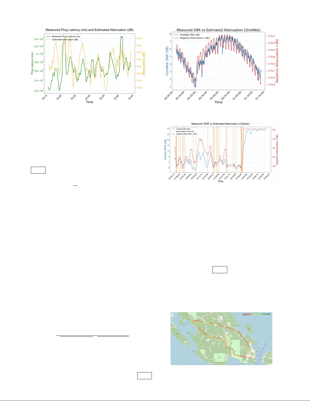
Scalable Air-to-Ground Wireless Channel Modeling Using Environmental Context and Generative Diffusion

1 Scalable Air -to-Ground W ireless Channel Modeling Using En vironmental Conte xt and Generati v e Dif fusion Jingyi T ian, Graduate Student Member , IEEE, Lin Cai, F ellow , IEEE, Abstract —The fast motion of Low Earth Orbit (LEO) satellites causes the propagation channel to vary rapidly , and its behavior is strongly shaped by the surr ounding en vironment, especially at low elev ation angles where signals ar e highly susceptible to terrain blockage and other en vironmental effects. Existing studies mostly rely on assumed statistical channel distributions and theref ore ignore the influence of the actual geographic en vironment. In this paper , we propose an en vironment-aware channel modeling method for air -to-gr ound wireless links. W e leverage real en vironmental data, including digital elevation models (DEMs) and land cover information, together with ray tracing (R T) to determine whether a link is line-of-sight (LOS) or non-line-of-sight (NLOS) and to identify possible reflection paths of the signal. The resulting obstruction and reflection profiles are then combined with models of diffraction loss, vegetation absorption, and atmospheric attenuation to quanti- tatively characterize channel behavior in r ealistic geographic en vironments. Since R T is computationally intensive, we use R T - generated samples and en vironmental features to train a scalable diffusion model that can efficiently pr edict channel performance for arbitrary satellite and ground terminal positions, thereby supporting real-time decision-making. In the experiments, we validate the proposed model with measurement data from both cellular and LEO satellite links, demonstrating its effectiv eness in realistic envir onments. Index T erms —LEO satellite, Channel Modeling, En vironment, T errain, Diffusion I . I N T RO D U C T I O N L Ow Earth Orbit (LEO) satellites operate at relati vely low altitudes, which significantly reduces propagation delay . Multiple satellites can further cooperate in constellations to provide global co verage, making LEO systems a key enabler of next-generation ubiquitous connectivity . Howe ver , their low orbital height also leads to high relativ e velocities with respect to ground user terminals (UTs), so the satellite–user geometry ev olves rapidly and the propagation channel becomes highly time-varying. As a result, link av ailability , capacity , and quality can change quickly , especially when the link is maintained at low ele vation angles where the line-of-sight (LOS) between the satellite and the UT passes close to the horizon and is thus prone to se vere blockage and frequent transitions to non- line-of-sight (NLOS) conditions. Under such highly time-varying conditions, the surrounding en vironment becomes a key factor in determining commu- nication performance. At lo w elev ation angles, the propa- gation path is more likely to intersect terrain, buildings, Parts of this paper were submitted to the IEEE International Conference on Communications (ICC) 2026 and are currently under revie w [1]. Jingyi T ian and Lin Cai are with the Department of Electrical and Computer Engineering, University of V ictoria, V ictoria V8P 5C2, Canada (e-mail: jingyit@uvic.ca, cai@uvic.ca). Fig. 1. Environment Illustration and vegetation, which can obstruct, attenuate, or scatter the signal, especially in the Ku/Ka bands that are widely used in LEO satellite communications and are highly sensiti ve to propagation impairments [2]. As a result, accurately captur- ing environmental effects on propagation is essential for the efficient and reliable operation of LEO satellite netw orks. Fig. 1 illustrates how en vironmental factors such as moun- tains, vegetation, sea surfaces, and buildings shape channel behavior . For some UT–LEO links, signals may be obstructed by mountains, ve getation, or buildings, leading to NLOS conditions with sev ere degradation, especially at low elev ation angles. Strong reflectors like sea surfaces induce multipath, while rainfall and clouds further impair link quality . Only when no obstruction exists between the satellite and the UT is the link considered LOS. The complexity of the en viron- ment highlights the need for an en vironment-aw are channel modeling method capable of capturing div erse influences on air-to-ground links. Ray tracing (R T) [3] is a deterministic channel modeling technique that computes electromagnetic propagation paths based on geometric optics, thereby reproducing signal prop- agation characteristics close to real conditions. It has been widely used in channel modeling. Ho we ver , most existing R T -based methods still rely on distributional assumptions, such as treating obstruction as a random v ariable [4], [5] or tuning abstract parameters to emulate different en vironments [6], leaving the actual en vironmental information explicitly unmodeled. Measurement-based approaches [7] better reflect reality b ut are costly and impractical in inaccessible regions such as polar areas. T o systematically ev aluate these en vironment-induced ef- fects, we choose the Canadian Arctic as our region of interest (R OI), which features di verse terrain (–109.9 m to 5083.8 m) [8] with mountain ridges, dense forests causing obstruction and absorption, strong reflectors such as sea and permanent ice surfaces, as well as residential buildings and barren lands, thereby offering a comprehensiv e set of en vironmental factors for ev aluation. Building on this R OI, we take two steps to address the gap that LEO satellite channel models rarely 2 account for the spatially v arying en vironment along the rapidly changing satellite–UT geometry . First, we construct a R T -based model using digital elev ation model (DEM) data [8], in which each pixel represents terrain elev ation, together with land co ver data [9] to determine NLOS links at the pixel lev el and record obstacles. W e compute terrain parameters (slope, aspect, roughness, curvature) and combine them with land cover to characterize surface reflec- tivity . W e then quantify dif fraction and extinction effects from terrain and vegetation obstructions, and multipath propagation from reflections. Meteorological data [10] are also used to quantify rain, cloud, and atmospheric attenuation, ensuring comprehensiv e en vironmental consideration. Second, across lar ge regions, the combinations of UT po- sitions with satellites at different altitudes, ele vations, and azimuths are effecti vely infinite, and the high computational cost of R T makes direct calculation infeasible for real-time use. T o tackle this, we first cluster the area by terrain, land cover , and functional types, then perform representative ground-point sampling within each cluster . Satellite altitude, elev ation, and azimuth are like wise sampled, and R T is ex ecuted only for these sampled UT–satellite pairs. Based on these samples, we train a diffusion model [11] to predict channels at arbitrary locations and geometries, thereby avoiding lar ge-scale, high- complexity R T computations. In summary , the main contrib u- tions of this paper are as follows: • En vironment-A ware Channel Modeling : W e integrate terrain, land cov er , and climate to determine their effects on signal propagation, enabling accurate air-to–ground link estimation. • Diffusion-Based Prediction : Channel performance is predicted from en vironmental inputs using a dif fu- sion model, replacing costly R T and enabling adaptiv e scheduling. • V alidation with Real Measurements : V alidation with real measured LEO satellite and cellular data demon- strates the model’ s accuracy and practical applicability . The remainder of this paper is organized as follo ws. Section II revie ws related work on wireless channel modeling. Sec- tion III presents the proposed site-specific channel modeling methodology , including region clustering and geometric chan- nel estimation. Section IV details the proposed diffusion-based prediction framew ork. Section V discusses the experimental setup and ev aluation results, and Section VI concludes the paper with future directions. I I . R E L A T E D W O R K W ireless channel modeling has been studied across ground, aerial, and satellite scenarios, e volving from purely statistical descriptions tow ard en vironment-aware methods. For ground- to-ground links, models are relatively mature. Recent work begins to incorporate environmental information and AI, for example, [12] combined building maps with R T -deriv ed LOS information and uses neural networks to predict urban path loss. Ho we ver , the scenario is restricted to flat city layouts. T er - rain undulation and rural/remote en vironments are not consid- ered, limiting generality beyond idealized urban grids. NIST’ s long-running measurement programs [7] collected extensi ve real-world data in typical urban and indoor en vironments, providing v aluable references for next-generation standards, but the campaigns are costly and geographically limited. Air-to-ground and air-to-sea modeling for UA V links is more recent and remains less mature. In maritime en viron- ments, [13] proposed a U A V–ship (U2S) MIMO channel model that incorporates sea clutter and wa ve shadowing com- bined with U A V 6D motion, but relies on Rayleigh-based fad- ing assumptions and lacks large-scale measurement support. For U A V -to-ground communications, [14] developed an ultra- wideband nonstationary model that combines geometry and R T to generate time-varying multipath components and jointly capture large and small-scale fading, yet its scenario di versity is limited and its dependence on full R T makes real-time use and large-area deployment challenging. In the agricultural IoUT setting, [15] augmented traditional path-loss models with empirical terrain, crop, and weather corrections, the en vironmental factors are introduced only as coarse correction terms and are not v alidated against independent measurements, making it difficult to assess robustness in more complex or unseen en vironments. Satellite-to-ground channel modeling is even more con- strained, with most studies focusing on low-ele vation degra- dation and often reverting to abstract statistics. Fle xible distribution-based models, such as the K-distribution for shad- owing in LEO direct-to-satellite links [4] and the η – µ shad- owed Ricean model for land-mobile satellite channels [5], can fit a range of fading behaviors but remain environment- agnostic and largely un v alidated by real measurements in div erse terrains. Hybrid approaches attempt to incorporate en vironment features through R T . [6] constructed simplified urban building and ve getation layouts and then fits elev ation- dependent distributions for dense city and residential areas, but still treats the ground as a flat plane and cannot represent real- istic terrain complexity . Recent learning-based works push fur- ther on prediction accuracy . [16] introduced a large language model (LLM)–based predictor for O TFS-enabled satellite–F AS links using historical channel coefficients, and [17] proposed a joint channel prediction and multibeam precoding method for LEO satellite IoT , trained on 3GPP deri ved simulated channel state information. These methods improve sequence prediction under long delays, yet they rely purely on synthetic or history- only channel coef ficients without e xplicitly modeling terrain, land cov er , or weather , raising concerns about generalization to real, heterogeneous environments. Overall, despite substantial progress from ground to U A V and satellite scenarios, most existing models still insufficiently capture real en vironments: terrain v ariations are often ignored or oversimplified, statistical abstractions dominate, measure- ment validation is rare or confined to limited regions, and heavy reliance on full R T makes large-scale, real-time use impractical. Field campaigns demonstrate the value of real measurements but are expensiv e and dif ficult to replicate in inaccessible areas, especially polar re gions. T o fill this gap, our work builds an e xplicitly en vironment- aware air–to–ground channel model dri ven by real geospatial information. W e integrate DEM, land cover data, and meteoro- 3 Fig. 2. Methodology Framework logical records to construct a realistic propagation en vironment that simultaneously accounts for terrain v ariation, surface type, and atmospheric conditions. W ithin this en vironment, R T is applied only to a set of sampled UT–satellite geometries, after which a diffusion model predicts channel states over the entire region, av oiding repeated large-scale R T in real-time operation. The approach is validated against measured data, sho wing that it captures en vironmental ef fects with high fidelity while supporting real-time applications and extending to previously inaccessible regions such as the Arctic. I I I . E N V I RO N M E N T - A W A R E C H A N N E L M O D E L I N G A. Overview W e propose an en vironment-aware air-to-ground channel modeling method and apply it in our R OI: Canada’ s Arctic which comprises Y ukon (YT), Northwest T erritories (NT) and Nunavut (NU), aiming to capture the impacts of comple x and div erse environments on LEO satellite channels. Fig. 2 sho ws the workflo w of the proposed approach. First, we extract terrain parameters such as slope from DEM data and apply the W eiss classification [19] scheme to catego- rize the terrain. These terrain classes are then combined with land cover types and land-use functions (e.g., protected areas, mining zones, residential settlements) to perform clustering on the R OI. Gi ven that direct computation of all satellite–UT links is infeasible, representativ e ground points—prioritizing high terrain elev ations and ridge-dense areas—are sampled in conjunction with satellite states spanning a range of ele vation angles, azimuths, and altitudes. Next, terrain parameters and land co ver to assess reflection capability of each pixel, producing a reflection map. W ith these information, we quantify signal loss for each link, including diffraction from terrain and vegetation obstructions, vegetation extinction, multipath from reflections, and atmospheric atten- uation from meteorological data, forming a comprehensiv e channel attenuation model. Instead of performing computationally intensiv e R T simula- tions for e very potential link at runtime, we train a diffusion- based predictor on sampled R T results and en vironmental features to estimate channel conditions at arbitrary locations, providing real-time inputs for scheduling decisions. The fol- lowing sections detail each design. B. Re gion Cluster 1) Re gion Cluster: The DEM data we used has a spatial res- olution of 10 × 10 meters per pixel. Based on our calculations, the R OI contains approximately 109.5 billion pixels. Since satellites at different altitudes operate with varying elev ation and azimuth angles, the number of possible link combinations between the satellites and UTs is ef fectiv ely infinite, making exhausti ve computation and storage impractical. T o ensure that the sampling points better reflect the characteristics of dif ferent en vironments instead of sampling randomly , we first cluster the entire region using en vironmental data: • T errain features: W e compute slope, aspect, roughness, curvature, T opographic Position Index (TPI), and T errain Ruggedness Index (TRI) from the DEM using RichDEM [18], and apply the W eiss classification method [19] to divide the terrain into valle ys, ridges, plains, and other categories based on flatness and slope. • Land cover features: The land cov er data of R OI contains 19 categories, including urban built-up areas, forests, shrubs, grasslands, and water/permanent ice, etc., with an overall accurac y of 86.9% [9]. • Functional region features: W e also use regional func- tional distribution data [20], which identifies the locations of residential areas, protected areas, mining regions, wilderness, etc., providing useful information about the relativ e density of UTs in dif ferent areas. Based on these information, we apply k-means clustering [21] to the entire region to guide the sampling for LOS and reflection calculations, ensuring that the distribution of sam- pling points accounts for the div erse environmental conditions. 2) Stratified sampling: Let the cluster set be C = { C 1 , . . . , C m } , Cluster C i contains N i candidate points, and the total number of candidates is N = P m i =1 N i . T o obtain samples that are both widely cov ered and representati ve under a fixed budget, we first allocate a sample quota to each cluster . The sampling weight of cluster C i is defined as: W i = ρ i · ( αω T + β ω F + γ ω L + δ ω E ) , (1) where ρ i = N i / N is the area (size) proportion of cluster C i , ω T , ω F , and ω L are the weighting factors for terrain type, functional region, and land cover , respecti vely , ω E is the elev ation gain factor , and the mixture coefficients satisfy α + β + γ + δ = 1 . By tuning these coefficients, one can realize task-specific sampling strategies, like LOS analysis or reflection analysis. Gi ven a total b udget S , the quota assigned to cluster is s i = S · W i P m j =1 W j . W ithin each cluster , we then select concrete samples accord- ing to its quota s i . Define a feature combination k = ( t, f , l ) , 4 where t , f , and l represent the terrain class, functional re- gion class, and land cover class, respectiv ely . The weight of combination k is: w k = ω T ( t ) × ω F ( f ) × ω L ( l ) , (2) and its allocated sample count is: s i,k = max  s min ,  w k P k ′ w k ′ · s i  , (3) where k ′ denotes all feature combinations that exist within cluster C i , s min enforces a minimum per-combination quota so that ev ery combination recei ves samples. W ithin each combination k , ground samples are selected uniformly at random, as points within the same combina- tion share similar en vironmental characteristics. T o prev ent excessi ve spatial clustering, we impose a minimum distance constraint d min so that the distance between any two retained samples is at least d min . This multi-stage stratified sampling strategy yields a sample set that (i) cov ers the main en viron- ment combinations, (ii) prioritizes more influential instances, and (iii) sufficiently spreads out in space. In practice, the coef ficients should be adjusted to the anal- ysis goal. For LOS blockage analysis, the allocation fav ors the terrain class α and terrain elev ation δ , and and assigning larger ω T to ridges/valle ys while do wn-weighting water in ω L to better capture ridges, valle ys, and other relief features that create obstructions. For reflection-path analysis, the allocation fa vors the land cover γ and boosting ω L for highly reflective classes, emphasizing strongly reflective areas. This parameter- ized design allows the same framew ork to adapt to multiple satellite-communication analysis scenarios. C. LOS and Reflection Map In our R OI, the elev ation values of DEM pixels range from − 109 . 9 m to 5083 . 8 m, indicating substantial relief. At low and moderate elev ation in a high relief region, satellite links are more susceptible to terrain obstruction. For K u/Ka bands commonly used in satellite communications, vegetation can also introduce notable attenuation. Therefore, for each DEM pixel we augment the terrain elev ation with a representativ e height of its overlying land cov er to form the pixel’ s ef fective terrain height . At each ground sampling location, we further generate multiple satellite positions: elev ation angles from 25 ◦ to 85 ◦ in 15 ◦ steps; azimuth angles from 0 ◦ to 300 ◦ in 60 ◦ steps; and three orbital altitudes of 500 km, 850 km, and 1200 km. W e implement a grid-based R T algorithm incorporating Earth-curvature correction and a Fresnel-zone criterion. T o ensure computational efficienc y over the large-scale R OI, a hierarchical traversal strategy is adopted. Since DEM products are typically provided as tiled datasets, the Liang-Barsky line- clipping algorithm [22] is first applied to rapidly identify the specific DEM data blocks intersected by the link vector . Subsequently , within each identified block, Bresenham’ s line algorithm [23] is employed to discretize the propagation path, strictly determining the raster pixels trav ersing the link. At each sampled pixel i , we first correct the link height to Fig. 3. Path Profile account for Earth curvat ure, which together make the Earth appear flatter . In the 4/3-Earth model the effecti ve radius is R eff = 4 / 3 × R ⊕ and R ⊕ is the physical Earth radius. The corrected link height is: H link = H raw link − d 1 d 2 2 R eff , (4) where d 1 , d 2 are the 3D distances from pix el i on the link to the satellite and the UT , respectiv ely . H raw link is the link height obtained by straight-line geometry between the UT and the satellite. W e compute the cl earance = H link − H terr ain which corresponds to the margin between the link height and the effecti ve terrain terrain height. The first-Fresnel-zone radius R 1 , which represents the region around the link where most of the signal energy propagates. For adequate clearance, the obstacle’ s normal distance to the link should be at least 0 . 6 R 1 . R 1 = r λ d 1 d 2 d 1 + d 2 , (5) where λ is the signal wa velength. Fig. 3 provides an intuitive illustration. The Fresnel clarity ratio is ρ = clearance × cos(elev ation) R 1 , (6) a negati ve value of the min clearance indicates that the link is obstructed. If min clearance ≥ 0 and ρ ≥ 0 . 6 , we classify the link as LOS; otherwise, it is NLOS. As in Algorithm 1, after classifying the link as LOS or NLOS, we construct a path profile P for NLOS links: the obstructed pixels on NLOS paths are ordered by horizontal distance to form a profile curve, and we record the clearance together with the location and height of each obstacle point. This provides both a global LOS/NLOS decision and the locations and heights of obstacles along the path, which will be used subsequently for channel estimation. In regions with ab undant water and permanent ice, signal re- flections are also non-negligible. Therefore, we first construct a reflection-capability raster based on the DEM and land cover data. As mentioned earlier , we compute slope S , roughness R , and curvature K from the DEM. After normalization, the terrain-based reflection score T is defined as: (7) where w S , w R , and w K are the respectiv e weights of slope, roughness and curvature. In this way , flat (lo w-slope) and 5 Algorithm 1 LOS/NLOS & Path Profile Construction Require: Coordinates of Start P s and End P e of a link; DEM Blocks D ; W avelength λ ; Effecti ve Earth Radius R eff Ensure: Output LOS/NLOS; path profile P P ← ∅ ; min clearance ← + ∞ ; min ρ ← + ∞ B intersect ← ∅ ; Pixel List ← ∅ /* Find intersected DEM blocks along the link */ B intersect ← LiangBarskyClipping ( P s , P e , D ) /* Find pixels along link */ for all Block b ∈ B intersect do L local ← BresenhamLine ( P s , P e , b ) Append L local to Pixel List end for for pix el i in Pix el List do Extract distance d 1 ( i ) , d 2 ( i ) and effecti ve terrain height H terrain ( i ) /* Earth-curvature corrected link height */ H link ( i ) ← H raw link ( i ) − d 1 ( i ) d 2 ( i ) 2 R eff /* Clearance and Fresnel clarity */ clearance ← H link ( i ) − H terrain ( i ) R 1 ← s λ d 1 ( i ) d 2 ( i ) d 1 ( i ) + d 2 ( i ) ρ ← clearance · cos θ R 1 min clearance ← min( min clearance , clearance ) min ρ ← min( min ρ, ρ ) if clearance < 0 or ρ < 0 . 6 then append ( dist h ( i ) , H terr ( i ) , clearance ) to P end if end for if min clearance ≥ 0 and min ρ ≥ 0 . 6 then retur n LOS, P = ∅ else sort P by dist h ascending retur n NLOS, P end if smooth (lo w-roughness) areas receiv e higher scores, and con- cav e regions (negati ve curv ature) are further enhanced. Next, land cover information is incorporated by assigning a linear attenuation coefficient β ℓ to each type. The final reflection coefficient is gi ven by: R = T · (1 + β ℓ ) . (8) In our settings, water surfaces are assigned β water = +0 . 50 to enhance reflection, while forests are assigned β forest = − 0 . 10 to attenuate reflection. The resulting reflection map provides a quantitativ e measure of spatial reflection potential, where larger values indicate stronger reflective capability , serving as input for multipath modeling. D. Channel Estimation In this section, we quantify channel losses from en viron- mental effects: climatic, obstruction, and multipath. For cli- matic effects, we apply ITU-R P .618 [24] using meteorological data [10] to model rain, cloud, and atmospheric attenuation, and incorporate these into the channel model. For obstruction effects, we consider two components: diffraction loss from terrain and land cover , and absorption loss from vegetation. Using the NLOS obstacle path profile, we apply the Delta- Bullington model [25] to compute diffraction loss. The model first determines obstacle positions and clearance heights, then sequentially ev aluates diffraction loss for each obstacle with ITU formulas, and finally transform multiple obstacles into an equiv alent single obstacle profile, on which the total dif fraction loss of the link is calculated. For vegetation loss, we sample along the path to reduce computational cost. Computing vegetation loss first requires the penetration distance through ve getation and the v egetation type. The challenge is to correctly identify the entry and exit of each vegetation segment. At each sampled point along the path we test the land cov er type. T o refine each entry/exit more accurately , we apply a bisection search, as described in Algorithm 2: if the current sample and its left neighbor share the same land-cover type, the boundary is on the left; if it matches the right neighbor , it is on the right. For vegetation segments V = { [ s ( k ) in , s ( k ) out , class ( k ) ] } k recorded along the path, where k = 1 , 2 , . . . index es segments. W e compute the penetration slant distance as s out − s in , where s denotes the cumulativ e slant path distance along the link, which is then passed to ITU-R P .833 model [26] with parameters adapted to frequency and land cover type. For multipath effects, enumerating all reflections is pro- hibitiv e. W e introduce a trade-off by sampling a circle around the UT with distance-dependent density , as LEO satellites transmit signals in beams. Reflection potential at sampled points is e valuated from the reflection map, and only high- potential candidates are retained. Among these, paths are validated by requiring the incident angle to equal the reflection angle. The TWDP model [27] is then applied to these validated paths, from which the direct path and the strongest reflection are selected to derive overall multipath gain/fading. Combined with free-space loss and other quantified effects, these results form the overall channel behavior . I V . D I FF U S I O N - B A S E D P R E D I C T I O N Exhaustiv ely modeling the near-infinite geometric combina- tions of ground points and moving satellites is computation- ally infeasible, while high-fidelity R T simulations remain too costly for real-time applications. T o address this, we employ diffusion models, which fundamentally operate by learning a rev erse denoising process—corrupting data structures with gradual noise during training and then learning to iterativ ely recov er complete samples from noisy or incomplete states. This generative mechanism of restoring order from disorder is inherently suited for reconstructing full fields from partial observations, aligning perfectly with our scenario. Specifically , we treat the en vironment map as a multi-channel image where limited channel loss observations are retained only at selected pixels, and we leverage the dif fusion model’ s capability in modeling spatial correlations to reconstruct the complete chan- nel information across the entire region, conditioned on these sparse inputs. 6 Algorithm 2 V egetation Se gmentation Detection Require: Input path distance s ∈ [0 , S max ] ; land-cover oracle T yp e( s ) ; sampling step ∆ s ; bisection tolerance ε Ensure: Output ve getation segments V = { [ s ( k ) in , s ( k ) out , class ( k ) ] } k V ← ∅ ; s ← 0 ; T prev ← Type(0) ; open ← false while s < S max do s next ← min( s + ∆ s, S max ) ; T ← Type( s next ) if T  = T prev then /* Boundary in ( s, s next ) by bisection */ L ← s ; R ← s next while R − L > ε do M ← ( L + R ) / 2 ; T M ← Type( M ) if T M = T yp e( L ) then R ← M else if T M = T yp e( R ) then L ← M else R ← M end if end while s ⋆ ← ( L + R ) / 2 ; T ⋆ ← Type( s ⋆ ) if T ⋆ is vegetation and ¬ open then /* ENTR Y */ s in ← s ⋆ ; class ← T ⋆ ; open ← true else if T ⋆ is non-vegetation and open then /* EXIT */ s out ← s ⋆ append [ s in , s out , class ] to V open ← false end if end if T prev ← T ; s ← s next end while if open then /* Path ends inside vegetation */ append [ s in , S max , class ] to V end if retur n V A. Input Repr esentation W e represent a region as a 3D tensor X ∈ R C × H × W , where C is the number of channels and H , W are spatial dimensions. The channels combine terrain, land-co ver , and geometry: C =  DEM , Slope , Aspect , LC emb  , The first four channels come from DEM, slope, aspect, and land cov er index. Since land over index is an integer label which carries no semantic information, using it directly may induce spurious correlations. Instead, for each pixel with class id c ∈ { 0 , . . . , K − 1 } , we map c to an E - dimensional continuous vector via a learnable embedding matrix W ∈ R K × E . The E components of embedded vector are then expanded along the channel dimension, forming LC emb 0 ..E − 1 ∈ R E × H × W , which are optimized end-to- end with the training loss. This allows the model to learn semantic proximity between classes under varying terrain and geometric conditions (e.g., grassland closer to shrubland), improving cross-region generalization. The DEM undergoes robust Min-Max scaling based on the 1 st and 99 th percentiles to suppress outliers, slope is linearly mapped to the [0 , 1] , while aspect is encoded via sine-cosine embeddings to resolve angular periodicity . Since the satellite geometric parameters are not pix el-lev el features, we combine them with the diffu- sion time-step embedding, and inject this joint embedding into ev ery layer of the U-Net [28] via residual blocks. B. Channel Loss Normalization W e consider channel conditions across v arious elev ation angles. At high elev ations, the excess loss for the majority of LOS links approaches zero. Meanwhile, in high-frequency satellite communication, obstacles cause loss v alues to instan- taneously span several orders of magnitude. Consequently , the observations exhibit a distinct mixed distribution characterized by zer o-inflation and heavy tails . In this context, standard linear normalization would be skewed by a few extreme deep-fading v alues, causing the dominant near-zero features to be compressed into an indistinguishably narrow numerical range, thereby hindering the model’ s ability to capture subtle fluctuations in LOS scenarios. Conv ersely , logarithmic scaling is undefined at zero and fails to smoothly adapt to the sharp transitions from LOS to NLOS conditions. T o address this, we design a transformation scheme based on the Robust In verse Hyperbolic Sine (Asinh) for the stan- dardization of channel loss observations. The Asinh facili- tates a smooth non-linear transition: in the low-loss regime ( m → 0 ), the function exhibits approximately linear behav- ior ( asinh( m ) ≈ m ), thereby meticulously preserving fine- grained details near the zero point; whereas in the high-loss regime ( m → ∞ ), it demonstrates logarithmic character- istics ( asinh( m ) ≈ ln(2 m ) ), compressing the heavy-tailed distribution associated with deep fading. Consequently , this design significantly enhances both the training stability and con ver gence rate of the diffusion model in complex hybrid scenarios. First, the ra w channel loss observations m dB are conv erted into linear power ratios m lin = 10 m dB / 10 . Subsequently , to align the input distribution with Asinh’ s linear-to-logarithmic transition, thereby simultaneously preserving subtle features near zero and compressing extreme values associated with deep fading, we introduce a scaling factor η to define the scaled linear power ratio ˜ m = m lin /η , which is subsequently processed by the inv erse hyperbolic sine transformation to obtain the intermediate variable n : n = arcsinh ( ˜ m ) , (9) where η is set to the 80 th percentile of the linear data distribution, serving to adaptiv ely determine the transition point between the linear and logarithmic regions. Finally , to mitigate the impact of outliers on the statistical distribution, we employ Z − S cor e standardization to obtain the final normalized channel observation z : z = n − µ σ , (10) 7 Fig. 4. Dual-Head U-Net where µ and σ represent the rob ust mean (the median of n ) and the robust standard deviation (deriv ed from the Interquartile Range of n ), respectively . C. Dual-Head U-Net Denoiser Giv en X and partially observed channel-loss field x 0 ∈ R 1 × H × W , we synthesize a noisy sample at timestep t : x t = √ ¯ α t x 0 + √ 1 − ¯ α t ϵ , ϵ ∼ N ( 0 , I ) , t = 1 → T , (11) ¯ α t is a predefined coefficient from the noise schedule that sets the signal–noise mixture at step t . ϵ is standard Gaussian white noise with the same shape as x 0 . W e feed noised target, conditioning map and diffusion timestamp ( x t , t, X ) into a U-Net denoiser f θ . The U-Net adopts an encoder–bottleneck–decoder architecture. Along the encoder path, residual blocks and strided con volutions re- peatedly downsample the feature maps from 32 channels at the original resolution to 64, 128, and 256 channels at progressiv ely lower spatial resolutions. This downsampling enlarges the receptiv e field and allo ws the network to capture broad spatial context at a manageable computational cost. The decoder then mirrors this process by upsampling the low- resolution features back to the original resolution (256 − → 128 − → 64 − → 32 channels), which enables precise, per- pixel predictions. Skip connections link encoder and decoder blocks at the same scale, so that high-resolution features from the contracting path are reused in the expanding path. When the channel is in LOS propagation state, its theoretical excess loss value should strictly be 0 dB. Howe ver , due to the aforementioned zer o-inflation issue, single-head regression models often struggle to con ver ge to a perfect zero during the final stage of denoising. This tendency results in residual non-zero v alues in unobstructed regions, creating background noise artifacts and blurring the boundaries of obstacles. T o further address this challenge, we propose a Dual-Head U- Net architecture as sho wn in Fig. 4. Both task heads share the same encoder -decoder backbone to extract generalized en vironmental features but bifurcate into two independent branches at the final output layer: 1) Regression Head: Outputs the continuous denoising target, responsible for quantifying the magnitude of the channel loss. 2) Classification Head: Outputs pixel-wise binary logits. Follo wing a Sigmoid activ ation, this yields a blockage probability map M prob ∈ [0 , 1] , which is used to explic- itly distinguish between LOS and NLOS states. These tw o distinct task heads are coupled at the pixel le vel through a soft-gating mechanism . The final channel loss field X final is formulated as: X final = X raw ⊙ ( M prob ) γ , (12) where X raw denotes the raw output of the regression head, ⊙ represents the Hadamard product, and γ is the gating intensity coefficient. Through this mechanism, the classification head functions as a learnable filter: in LOS regions where M prob → 0 , the regression output is suppressed to zero; conv ersely , in obstructed regions where M prob → 1 , the regression value is preserved. This strategy not only eliminates background artifacts but also significantly sharpens the boundaries of obstacles. Conditioned on both t and the satellite geometry (SatGeo) at e very resolution le vel, the network is tasked with denoising. T o enhance the numerical stability of geometric data reconstruction, we transition from the standard noise prediction target ( ϵ -prediction) to v-parameterization . In this formulation, we define the ground truth velocity target v t in the latent space as a linear combination of the clean signal x 0 and noise ϵ : v t ≡ α t ϵ − σ t x 0 , (13) Unlike ϵ -prediction, v-parameterization provides consistent gradient estimates across the entire diffusion trajectory . The network f θ is trained to approximate v t . The training objectiv e minimizes the loss function: L = E t, x 0 ,ϵ  λ t ∥ v t − f θ ( x t , t, X ) ∥ 2 + λ cls L cls  , (14) where L cls denotes the binary cross-entropy loss of the clas- sification head. The total objective comprises two terms: a regression loss weighted by the time-dependent coef ficient λ t , and the classification loss scaled by the hyperparameter λ cls . D. Infer ence In the inference phase, the model initiates from pure Gaussian noise x T ∼ N ( 0 , I ) and iterativ ely recovers the signal over t = T → 1 using a DDIM sampler [29]. W e enforce a Physics-Informed Inpainting Strate gy to ensure the 8 reconstructed field remains strictly anchored to the sparse site- specific ground truth. At each timestep t , the network predicts the velocity field f θ ( x t , t, X ) . Under the v-parameterization scheme, we first estimate the clean signal ˆ x 0 from the current noisy state x t via the linear transformation: ˆ x 0 ( x t , t, X ) = √ ¯ α t x t − √ 1 − ¯ α t f θ ( x t , t, X ) . (15) Based on this ˆ x 0 , the DDIM sampler proposes a denoised latent state x pred t − 1 for the next timestep. Howe ver , directly retaining this prediction allows de viations from the observed physical reality . Since the intermediate state x t − 1 resides in a high-noise manifold, inserting noise-free data creates a sev ere SNR discontinuity at the boundaries. This distrib ution mismatch destabilizes the U-Net, leading to incoherent arti- facts. T o resolve this, we perform a re-noising and masking operation: 1) Re-noising: W e project the sparse clean observations x obs 0 into the same noise manifold as the current timestep t − 1 by adding Gaussian noise matching the schedule intensity , ensuring statistical consistency with the sur- rounding generated regions: x known t − 1 = √ ¯ α t − 1 x obs 0 + p 1 − ¯ α t − 1 ϵ, ϵ ∼ N ( 0 , I ) (16) 2) Masking: Using the binary observation mask M , we fuse the model’ s prediction with the re-noised ground truth to obtain the final state for the next iteration: x t − 1 = x pred t − 1 ⊙ (1 − M ) + x known t − 1 ⊙ M . (17) Through this iterative correction, accurate physical infor- mation effecti vely diffuses into unobserved regions without introducing boundary artifacts, guiding the model to synthe- size a full-field channel loss map that is both geometrically consistent and physically accurate. V . E V A L UA T I O N A. Evaluation on Real Datasets Using real datasets [8]–[10] and our method, we computed obstruction, reflection, and attenuation maps for the R OI. Fig. 5a shows obstruction rates at different elev ations: they stay low at high elev ations, both due to the natural advantage of elev ation and the diluting effect of e xtensiv e flat plains, while rates are higher in the northeast with rugged ice terrain and in the southwest with dense forests and residential areas. The rate rises sharply at lo wer ele vations, reaching 24.28% at 25° ev en with the presence of extensiv e plains, which significantly impacts link reliability . Fig. 5b sho ws the reflection map, with weaker reflection in southwest forests and northeast rugged terrain but stronger in the central flat area, consistent with the obstruction distribution. Fig. 6 further sho ws the distribution of channel attenuation at dif ferent elev ation angles. The results indicate that attenua- tion is concentrated in the northern and southern parts of the R OI, while it is negligible in the central region. This spatial heterogeneity rev eals the regionalized impact of en vironmental factors on channel quality and provides a quantitativ e basis for resource scheduling and link management. Consequently , systems can anticipate cov erage of high-attenuation regions and proacti vely implement dynamic resource allocation and optimization, thereby enhancing ov erall network performance and service reliability . (a) Obstruction rate. (b) Reflection map . Fig. 5. Obstruction rate and reflection map. (a) 25 ◦ (b) 40 ◦ (c) 55 ◦ (d) 70 ◦ (e) 85 ◦ Fig. 6. Attenuation heat map at different elevation. B. V alidation T o validate the effecti veness of our method, we conducted ev aluations using real-world data from Starlink [30], OneW eb [31], and cellular networks. W e discuss the results for each validation set in the following sections. 1) Starlink: As Starlink is currently the most mature satellite constellation, we compared model-estimated signal attenuation with real measured Starlink UT ping latency from the LENS dataset [32], smoothed with a 60-second moving av erage to better observe ov erall trends and mitigate random noise. W e use the Seattle subset of the LENS dataset, which shows noticeable obstruction despite UTs usually being de- ployed in open sites, making it representativ e. DEM [33] and land co ver data [34] of Seattle were then used to estimate the channel condition at the UT location. Since Starlink dishes do not provide access to channel qual- ity measurements, we must rely on end-to-end Ping measure- ments to infer channel performance. In Fig. 7, the yello w curve shows model-estimated signal attenuation (dB) and the green curve shows measured ping latency (ms) over 30 minutes. The changing signal attenuation was mainly due to the mobility 9 Fig. 7. V alidation on Starlink. of the satellite, resulting in changing elev ation angles and obstructions. Though not directly comparable, Ping message delay reflects channel behavior and both exhibit consistent trends. T o quantify this, we employed Sign Agr eement , since the two metrics dif fer in units and scales. It measures the proportion of instances where estimated ( x i ) and measured ( y i ) values change in the same direction. The correlation coefficient of 0.734 indicates a strong correlation. Sign Agreement = 1 N N X i =1 1  sign ( x i ) = sign ( y i )  , (18) Direct verification with Starlink is challenging, since its per- satellite downlink is characterized in terms of aggregate capac- ity , while phased-array beamforming dynamically reallocates beams and capacity to match demand [35], so the observed ping latenc y is af fected by scheduling and beam management in addition to the physical channel state, and thus cannot reliably represent instantaneous channel conditions. 2) OneW eb: OneW eb serves as another key constellation for v alidation as it e xposes SNR readings to UTs. T o directly validate our channel model using this metric, we compared the model-estimated signal attenuation with the OneW eb SNR collected in [36]. W e applied our model to the en vironmental data [33], [34] at corresponding locations, and the results are illustrated in Fig. 8. A strong correlation is observed between the OneW eb SNR (blue curve, dB) and the estimated atten- uation (red curve, dB). Noting that attenuation and SNR are negati vely correlated—where higher attenuation corresponds to lower SNR—we inv erted the estimated attenuation values to align the visual trends. Given that both metrics are in the same dimension (dB), we employed the P earson correlation coefficient to quantify their linear correlation. r = P N i =1 ( x i − ¯ x )( y i − ¯ y ) q P N i =1 ( x i − ¯ x ) 2 q P N i =1 ( y i − ¯ y ) 2 , (19) where x i and y i denote the predicted and measured values, ¯ x and ¯ y their means, and N the number of samples. Statistical significance is assessed by the p-v alue from the t -distrib ution with N − 2 degrees of freedom, where p < 0 . 05 is generally considered significant. Our correlation coefficient of 0.906 Fig. 8. V alidation on OneW eb . Fig. 9. V alidation on Cellular. with p = 0 shows strong consistency between estimated and measured values. 3) Cellular: W e conducted cellular tests on Galiano Island, Canada, collecting L TE SNR while traveling [37]. Using DEM [38] and land cover data [9], our method estimated channel conditions at the corresponding GPS locations. Fig. 9 shows the results: the red curve is estimated loss (dB), the blue curve is measured L TE SNR (dB), and the vertical orange lines mark base station handov ers. Fig. 10 shows the actual dri ving route along which the measurements were collected. The P earson correlation coefficient of 0.932 with p = 0 shows strong consistency between estimated and measured values. While the measurements are affected by user behavior and base station power differences, the results sufficiently v alidate the feasibility of the proposed method. Fig. 10. Trajectory Map. 10 C. Pr ediction Accuracy of Diffusion Model T o assess the capability of the proposed diffusion model in reconstructing full-field channel maps within complex geographical en vironments, this section e valuates prediction performance across varying degrees of observation sparsity . Giv en the highly complex and significantly heterogeneous surface and geometric features of the large-scale R OI, direct training on the entire area risks introducing data redundancy and compromising result interpretability . Consequently , we selected three representati ve and distinct 30 × 30 km sub- regions with distinct features: • Region A: flat terrain with a standard de viation of 18.2 m in elev ation and essentially no ve getation, representati ve of open, unobstructed land. • Region B: moderate relief with an ele vation standard deviation of 563.2 m and approximately 29.9% ve getation cov erage, capturing hilly areas with a mix of obstructed and unobstructed paths due to both terrain undulation and forested regions. • Region C: rugged terrain with an elev ation standard deviation of 701.8 m and no vegetation, representing steep mountain regions. T o ev aluate dif ferent levels of observ ation sparsity , we sample approximately 1% and 4% of the pixels in each sub- region. Our model was then applied to these sampled points to obtain the raw observations. For conv olutional stability , subre- gions are formed into 256 × 256 pixel tiles, where channel-loss observations are georeferenced with environmental features and satellite geometry . The model is trained for 500 epochs (batch size = 16) with a 250-step diffusion process. (a) sample rate = 1%. (b) sample rate = 4%. Fig. 11. Conv ergence curve. Fig. 11 illustrates the loss con vergence curve of the model ov er the first 100 training epochs. As observed, there is a rapid decline in training loss during the initial phase. This is attributed to the implementation of a Curriculum Learning strategy: for the first 10 epochs, the model is fine-tuned exclusi vely on low-noise intervals, after which the training is extended to the full range of 250 noise diffusion steps starting from the 11th epoch. This design aims to prevent the model from being e xposed directly to high-variance pure noise images during the parameter initialization stage, which could cause it to degenerate into a trivial solution of merely outputting the statistical mean to minimize global error . Consequently , a transient rise in loss occurs at the 11th epoch upon the transition in difficulty level. Nev ertheless, this is a normal adjustment follo wing the increase in task complexity and does not af fect the overall con vergence trend, Fig. 12. Diffusion model performance when sample rate = 1%. Fig. 13. Diffusion model performance when sample rate = 4%. demonstrating the model’ s robust optimization stability . No- tably , while the curve appears to descend more rapidly when using only sparse data (Fig. 11a), this is essentially an ar- tifact indicati ve of ov erfitting, suggesting the model lacks the genuine generative capacity to handle complex v ariations. Con versely , the fluctuations observed in the conv ergence curve with denser observations (Fig. 11b) reflect the model’ s tran- sition from ”rote memorization” to a true ”understanding” of the feature distribution. Fig. 12 and Fig. 13 compare the predicted Mean Absolute Error (MAE) across three sub-regions under dif ferent sampling densities: a sampling rate of approx. 1% and a sampling rate approx. 4%, respectiv ely . It shows that increasing the sampling density significantly reduces prediction errors, particularly in scenarios characterized by low elev ation angles and rugged terrain. For instance, in Region C, the MAE drops drastically from 5.22 dB to 1.23 dB — a reduction of approximately 76.4%. In contrast, at high elev ation angles, the link is nearly vertical and thus less susceptible to en vironmental obstruc- tions, the MAE in these cases remains consistently lo w and is less sensitiv e to changes in sampling density . W e further compare the computational efficienc y between the R T method and the diffusion-based inference. For a 256 × 256-pixel tile (65,536 pixels in total), R T computation re- quires roughly 144000 seconds , whereas the dif fusion model completes forw ard inference in about 300 seconds . Overall, despite small accuracy degradation, it substantially reduces the total computational cost. Results in Fig. 12 and Fig. 13 also indicate that the extent of pre-calculation can be flexibly 11 determined based on the specific accuracy requirements of different tasks. V I . C O N C L U S I O N This paper presents an en vironment-aware air-to-ground channel modeling method that integrates terrain, land cover , and climate data to estimate channels, validated with real- world measurements. A dif fusion model further predicts chan- nel states for arbitrary UT–satellite pairs, reducing reliance on ray tracing and making our solution more scalable. The proposed model can support resource scheduling and link management, offering practical v alue for network deployment and optimization. For future work, we will refine the model to better capture seasonal ve getation dynamics, v alidate it across div erse en vironments, and incorporate it into LEO network resource management and enhance hando ver performance. A C K N O W L E D G M E N T The authors would like to thank Dr . Jianping Pan, Jinwei Zhao and Finnegan Archer for their assistance in the collection of real-world measurement data. R E F E R E N C E S [1] Jingyi T ian, Lin Cai, ”Scalable Air -to-Ground W ireless Channel Modeling Using En vironmental Context and Diffusion Models, ” IEEE International Conference on Communications (ICC) 2026, under review . [2] ITU-R, “Prediction of clutter loss (30 MHz–100 GHz), ” Recommenda- tion ITU-R P .2108-1, International T elecommunication Union, Gene va, Switzerland, Aug. 2017. [3] 3GPP , “Study on channel model for frequencies from 0.5 to 100 GHz, ” 3GPP TR 38.901, v14.0.0, Release 14, 2017. [4] T . N ´ u ˜ nez-Gonz ´ alez, et al. “Enhancing LEO direct-to-satellite channel modeling with the shadowing effect via K-distribution. ” ICT Express (2025). [5] S. Panic, et al. “On the η - µ shadowed Ricean model for land mobile satellite channels. ” Annals of T elecommunications (2025): 1-7. [6] W . Khaw aja, et al. “Propagation Channel Modeling for LEO Satellite Mis- sions Using Ray-Tracing Simulations. ” arXiv preprint (2025). [7] National Institute of Standards and T echnology (NIST), U.S. Department of Commerce. [Online]. A vailable: https://www .nist.gov/ [8] C. Porter, et al., “ ArcticDEM, V ersion 4.1. ” Harv ard Dataverse, V1, 2023. https://doi.org/10.7910/D VN/3VDC4W . [9] Government of Canada, “2020 Land Cover of Canada. ” Natural Resources Canada, 2020. [Online]. A vailable: https://open.canada.ca/data/en/dataset/ee1580ab-a23d-4f86-a09b- 79763677eb47. [10] En vironment and Climate Change Canada (ECCC), ”Historical Climate Data, ” Government of Canada. [Online]. A vailable: https://climate.weather .gc.ca/ [11] J. Ho, A. Jain, and P . Abbeel, “Denoising dif fusion probabilistic models, ” in *Proc. Adv . Neural Inf. Process. Syst. (NeurIPS)*, vol. 33, pp. 6840–6851, 2020. [12] R. He, et al. “COST CA20120 INTERACT framework of artificial intelligence-based channel modeling. ” IEEE Wireless Communications (2025). [13] N. Ahmed et al., “Impact of sea cluttering and wave shadowing on U2S MIMO channel model incorporating U A V–ship 6D motion in maritime en vironments, ” V eh. Commun., vol. 55, art. no. 100963, 2025. [14] B. Hua et al., “Ultra-wideband nonstationary channel modeling for U A V - to-ground communications, ” IEEE T rans. Wireless Commun., vol. 24, no. 5, pp. 4190–4204, May 2025. [15] W . Ahmad et al., “IoUT and collaborativ e cloud computing based U A V channel modeling for agriculture communication, ” IEEE T rans. Consum. Electron., early access, Aug. 2025, doi: 10.1109/TCE.2025.3593867. [16] H. Y ang, et al. “F AS-LLM: Large Language Model-Based Chan- nel Prediction for OTFS-Enabled Satellite-F AS Links. ” arXiv preprint arXiv:2505.09751 (2025). [17] M. Y ing, et al. “Deep learning-based joint channel prediction and multi- beam precoding for LEO satellite Internet of Things. ” IEEE Transactions on Wireless Communications 23.10 (2024): 13946-13960. [18] R. Barnes, “RichDEM: T errain Analysis Software, ” 2016. [Online]. A vailable: http://github .com/r-barnes/richdem [19] A. W eiss. “T opographic position and landforms analysis. ” Poster pre- sentation, ESRI user conference, San Diego, CA. V ol. 200. 2001. [20] Government of Canada, “Functional Region / Land Use Function Distribution Dataset, ” Open Data Portal, 2023. [Online]. A vailable: https://open.canada.ca/data/en/dataset/7e388083-6b66-5e0e-a264- a3c0eb98a2f0 [21] F . Pedregosa, et al. “Scikit-learn: Machine learning in Python. ” the Journal of machine Learning research 12 (2011): 2825-2830. [22] Y .-D. Liang and B. A. Barsk y , “ A new concept and method for line clipping, ” A CM Trans. Graph., vol. 3, no. 1, pp. 1–22, Jan. 1984. [23] J. E. Bresenham, “ Algorithm for computer control of a digital plotter , ” IBM Syst. J., vol. 4, no. 1, pp. 25–30, 1965. [24] ITU-R, “Propagation data and prediction methods required for the design of Earth-space telecommunication systems, ” Rec. ITU-R P .618-14, 2022. [25] ITU-R, “Prediction procedure for the ev aluation of interference between stations on the surface of the Earth at frequencies above about 0.1 GHz, ” Recommendation ITU-R P .452-18, International T elecommunica- tion Union, Genev a, Switzerland, Oct. 2023. [26] ITU-R, “ Attenuation in vegetation, ” Recommendation ITU-R P .833-10, International T elecommunication Union, Genev a, Switzerland, Sep. 2021. [27] G. Durgin, et al. “New analytical models and probability density functions for fading in wireless communications. ” IEEE Transactions on Communications 50.6 (2002): 1005-1015. [28] O. Ronneberger , et al. “U-Net: Con volutional networks for biomedical image se gmentation. ” International Conference on Medical image com- puting and computer-assisted intervention. Cham: Springer international publishing, 2015. [29] J. Song, et al. “Denoising diffusion implicit models. ” arXiv preprint arXiv:2010.02502 (2020). [30] SpaceX, “Starlink, ” [Online]. A vailable: https://www .starlink.com/. [31] OneW eb, “Our network (High-speed, low-latency LEO satellite), ” OneW eb, n.d. [Online]. A vailable: https://oneweb .net/our-network. [32] J. Zhao, and J. Pan. “LENS: A LEO satellite network measurement dataset. ” Proceedings of the 15th ACM Multimedia Systems Conference. 2024. [33] U.S. Geological Survey , “1 Arc-second Digital Elev ation Models (DEMs) - USGS National Map 3DEP Downloadable Data Collection, ” USGS Science Data Catalog, 2024. [Online]. A vailable: https://data.usgs.gov/datacatalog/data/USGS%3A35f9c4d4-b113-4c8d- 8691-47c428c29a5b . [34] United States Geological Surve y , “ Annual National Land Cov er Database (NLCD) Collection 1.0 Reference Data Product, ” U.S. Geological Survey , Data Release, Jul. 25, 2025. [Online]. A vailable: https://www .usgs.gov/data/annual-national-land-cover -database-nlcd- collection-10-reference-data-product. [35] Space Exploration Holdings, LLC, “ Application for Approval for Orbital Deployment and Operating Authority for the SpaceX NGSO Satellite System—Attachment: Legal Narrative, ” IBFS File No. SA T - LO A-20161115-00118, filed Nov . 15, 2016. [Online]. A v ailable: https://fcc.report/IBFS/SA T -LOA-20161115-00118/1158349.pdf [36] J. Zhao, O. Perrin, A. Ahangarpour and J. Pan, ”Measuring the OneW eb Satellite Network, ” 2025 9th Network Traf fic Measurement and Analysis Conference (TMA), Copenhagen, Denmark, 2025, pp. 1-10. [37] F . Archer , “ Analyzing the broadband divide in the underserved Southern Gulf Islands, ” poster , Univ ersity of V ictoria, V ictoria, BC, Canada, 2025. Online. A v ailable: https://hdl.handle.net/1828/22560. [38] Government of BC, “Map Series, ” ArcGIS Online. [Online]. A vailable: https://governmentofbc.maps.arcgis.com/apps/MapSeries/inde x.html.