Manifold Generalization Provably Proceeds Memorization in Diffusion Models

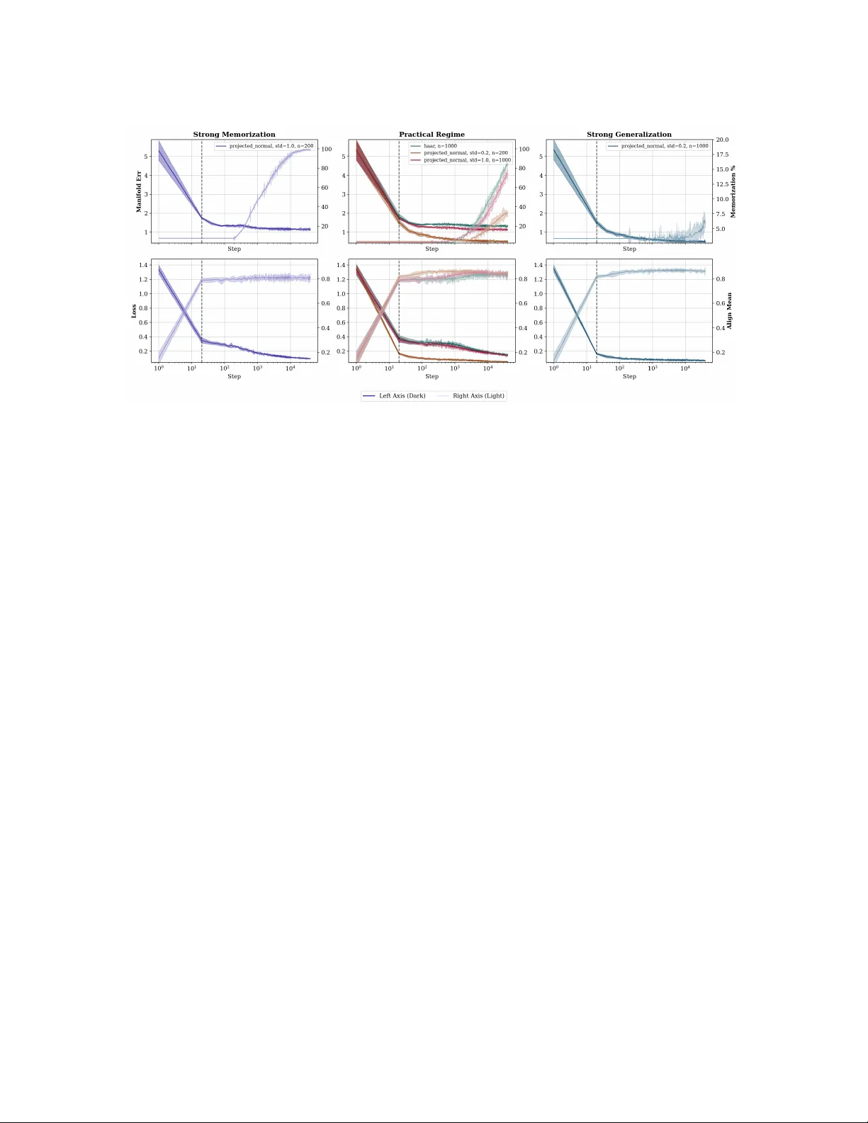
1 – 62 Manif old Generalization Pro vably Proceeds Memorization in Diffusion Models Zebang Shen ⋆ Z E BA N G . S H E N @ I N F . E T H Z . C H Y a-Ping Hsieh ⋆ Y A P I N G . H S I E H @ I N F . E T H Z . C H Niao He N I AO . H E @ I N F . E T H Z . C H ETH Zurich Abstract Diffusion models often generate nov el samples ev en when the learned score is only coarse —a phenomenon not accounted for by the standard vie w of diffusion training as density estimation. In this paper , we sho w that, under the manifold hypothesis , this behavior can instead be e xplained by coarse scores capturing the geometry of the data while discarding the ﬁne-scale distrib utional structure of the population measure µ data . Concretely , whereas estimating the full data distribution µ data supported on a k -dimensional manifold is known to require the classical minimax rate ˜ O ( N − 1 /k ) , we prov e that diffusion models trained with coarse scores can exploit the r egularity of the manifold support and attain a near-parametric rate to ward a dif ferent target distribution. This target distribution has density uniformly comparable to that of µ data throughout any ˜ O  N − β / (4 k )  -neighborhood of the manifold, where β denotes the manifold regularity . Our guarantees therefore depend only on the smoothness of the underlying support, and are especially fa vorable when the data density itself is irregular , for instance non-dif ferentiable. In particular, when the manifold is sufﬁciently smooth, we obtain that generalization —formalized as the ability to generate novel, high-ﬁdelity samples—occurs at a statistical rate strictly faster than that required to estimate the full population distribution µ data . Keyw ords: diffusion models; score matching; manifold hypothesis; co verage; minimax rates. 1. Intr oduction Dif fusion and score-based generativ e models deliv er striking sample quality in high-dimensional domains ( Ho et al. , 2020 ; Song et al. , 2021 ; Dhariwal and Nichol , 2021 ; Rombach et al. , 2022 ; Karras et al. , 2022 ). Y et a persistent empirical pattern is that genuinely novel samples—outputs that are not mere near-duplicates of the training set—often emerge only when the learned score is coarse , for instance under early stopping or limited model capacity ( Gu et al. , 2023 ; Somepalli et al. , 2023 ; Bonnaire et al. , 2025 ; Achilli et al. , 2025b ). This seems at odds with the dominant theoretical paradigm, which treats diffusion training as a density estimation problem and establishes sampling or con vergence guarantees under suf ﬁciently accurate score/denoiser estimation, typically in large-sample regimes ( T ang and Y ang , 2023 ; Lee et al. , 2023 ; De Bortoli , 2022 ; Oko et al. , 2023 ; Azangulov et al. , 2024 ; Chen et al. , 2023 ). In that view , improving score accuracy should monotonically improv e approximation to the population distribution. W e therefore ask: How can an inaccurate scor e still yield non-memorized , high-quality samples? W e study this question under the manifold hypothesis ( Fefferman et al. , 2016 ): data concentrate on a k -dimensional C β submanifold M ⋆ ⊂ R D with k ≪ D . Our thesis is that the rele vant objectiv e behind “generalization” is often not minimax reco very of the full density µ data , but rather coverag e of M ⋆ at a nontri vial spatial resolution. ⋆ Equal contribution. © Z. Shen, Y .-P . Hsieh & N. He. S H E N H S I E H H E A coverage criterion. Fix δ > 0 . Informally , we say that a distribution µ has δ -cover age of µ data if there exists a constant c > 0 , independent of the sample size, such that for ev ery y ∈ M ⋆ := supp( µ data ) , µ  B M ⋆ δ ( y )  ≥ c µ data  B M ⋆ δ ( y )  , where B M ⋆ δ ( y ) is the geodesic ball of radius δ on M ⋆ . This formalizes the requirement that µ does not “miss” any re gion of M ⋆ that is non-negligible under µ data at resolution δ . In this light, the empirical distribution µ emp faces a fundamental obstruction: the smallest δ for which µ emp ( B M ⋆ δ ( y )) > 0 for all y scales as ˜ O ( N − 1 /k ) . In contrast, our main ﬁnding is that diffusion sampling with a coarsely learned score can nonetheless yield distributions with muc h ﬁner on-manifold coverage. Theorem 1 (Main; inf ormal) Assume µ data is supported on a k -dimensional C β submanifold M ⋆ ⊂ R D and satisﬁes mild r e gularity conditions. Given N i.i.d. samples fr om µ data , consider a diffusion model trained only to coarse scor e accuracy . Then, with high pr obability , the induced sampling dynamics ar e ˜ O ( N − 1 ) -close in squar ed Hellinger distance to a distrib ution that achie ves δ -cover age at the scale 1 δ = ˜ O  N − β / 4 k  . In particular , when the smoothness parameter β > 4 , diffusion sampling achie ves strictly ﬁner on-manifold cov erage while learning only a cover ed surr ogate at a near-parametric rate ˜ O ( N − 1 / 2 ) . Operationally , this means that the resulting samples lie (approximately) on the underlying data manifold while remaining far from an y indi vidual empirical datapoint. In this sense, diffusion models achie ve gener alization : they produce no vel, high-quality samples without memorizing the training set. Intuition and technical highlights. Let µ t : = µ data ∗ N (0 , tI D ) denote the Gaussian-smooth data measure and let Pro j M be the nearest-point projection onto M ⋆ (well-deﬁned on a tub ular neighborhood of M ⋆ ). A central object in our analysis is the smooth–then–pr oject distribution µ pro j : = Pro j M # µ t = Pro j M #  µ data ∗ N (0 , tI D )  . ( µ pro j ) Intuiti vely (and will be made precise in Theorem 7 ), when t lies in a moderate re gime, µ pro j serves as a canonical cover ed surr ogate for µ data . Moreover , the two operations deﬁning µ pro j —Gaussian smoothing and geometric projection—each enjoy fa vorable statistical properties: 1. Smoothing is statistically cheap. Although µ emp is a poor proxy for µ data at ﬁne scales, Gaussian smoothing makes the estimation pr oblem essentially parametric : for any ﬁxed t > 0 , KL( µ t ∥ µ emp ∗ N (0 , tI D )) = ˜ O ( N − 1 ) , where ˜ O ( · ) hides constants depending on t and M ⋆ ; see Theorem F .1 . This estimate in turn implies that the dif fusion model can be learned quickly , in Hellinger distance, to ward a distribution that approximates µ pro j deﬁned in ( µ pro j ); see Theorem 2 . 2. Geometry is easier than full density estimation. Approximating µ pro j primarily requires recov ering the projection map Pro j M , a geometric object that can be estimated at rates signiﬁcantly faster than reco vering µ data . 1. W e focus on the smoothness parameter β , leaving the impro vement of the factor 4 in the denominator to future work. 2 M A N I F O L D G E N E R A L I Z A T I O N P RO V A B LY P RO C E E D S M E M O R I Z A T I O N I N D I FF U S I O N M O D E L S Figure 1: Geometry precedes memorization in diffusion training. T op r ow: training dynamics across three regimes. The manifold error (dark, left axis) decreases rapidly , while the memorization rate (light, right axis) stays low for coarsely optimized scores. The “gener- alization” windo w is the regime where both manifold error and memorization are small. Bottom r ow: our diagnostic for manifold learning . Alongside the training loss (dark, left axis), we report the mean alignment (light, right axis) between the learned score s θ and the projection direction, ⟨ Pro j M , s θ ⟩ / ( ∥ Pro j M ∥ ∥ s θ ∥ ) . Across regimes, alignment rises quickly and saturates early , suggesting that the coarse score network ﬁrst recovers manifold geometry , while memorization is a later-stage ef fect. T ogether , these suggest that learning µ pro j can be substantially easier than learning µ data in the minimax sense, while still being suf ﬁcient for producing non-memorized, high-quality samples. Our approach. Motiv ated by these observations, we decompose the analysis into two noise regimes. In the moderate-to-large noise regime ( t ≥ t 0 for a manifold-dependent threshold t 0 ), we assume suf ﬁciently accurate score learning. In this range, training effecti vely tar gets the Gaussian-smoothed empirical law µ emp ∗ N (0 , t 0 I D ) and thus yields a near-parametric approximation of µ t 0 by the preceding discussion; this is the “easy” regime. Our main technical contrib ution is in the small-noise re gime, where the objecti ve is g eometric recov ery rather than distributional learning (see Figure 1 for empirical e vidence and Section F .1 for experimental details): For a function class chosen to reﬂect both theory and this empirical behavior , we show that a coarsely learned score—when coupled with the ODE inte grator most commonly used in practice (rather than the elementary rev erse-time SDEs)—implicitly realizes an approximate projection map Pro j c M . Quantitati vely , this yields a manifold estimator c M with Hausdorf f and projection accuracy ( Theorem 3 and Theorem 4 ) d H ( c M , M ⋆ ) = ˜ O  N − β /k  , ∥ Pro j M − Pro j c M ∥ ∞ = ˜ O  N − β / (2 k )  . A geometric transfer step then conv erts projection accuracy into δ -cov erage at intrinsic scale δ = ˜ O  N − β / (4 k )  ; see Theorem 7 . 3 S H E N H S I E H H E Literature Re view Minimax manif old estimation vs. diffusion theory . A classical line of work de velops minimax- optimal rates for estimating (i) an embedded manifold M ⋆ and its local geometry ( Aamari and Le vrard , 2019 ) and (ii) measures supported on M ⋆ , under reach and C β regularity assumptions; see, e.g., ( Di vol , 2022 ). More recent diffusion theory adapts parts of this minimax toolkit to obtain sharp distributional recov ery guarantees for diffusion models ( Oko et al. , 2023 ; Azangulov et al. , 2024 ; T ang and Y ang , 2024 ). Howe ver , this literature does not address our motiv ating puzzle—why only coarse scores can still yield novel , high-quality samples—and it does not provide ﬁnite-sample guarantees phrased in terms of on-manifold covera ge . In particular , to the best of our knowledge, no existing w ork establishes minimax-style rates for manifold (or pr ojection) estimation via dif fusion models . Finally , we emphasize that our coarse-score requirement ( Assumption 2 ) alone cannot guarantee distributional recov ery , since it may hold for two very different distributions µ data and µ ′ data as long as they share the same support. More concretely , and to put our result in perspective, it is natural to compare it with the classical minimax rate for estimating the full data distribution µ data . For an α -smooth density supported on a k -dimensional domain, the optimal rate scales as ˜ O  N − α/k  ( Di vol , 2022 ; Achilli et al. , 2025a ; T ang and Y ang , 2024 ). This benchmark assumes that µ data itself admits an α -smooth density , whereas our guarantees instead rely on the geometric re gularity of the underlying manifold. In particular , the density smoothness α is typically smaller than the manifold re gularity β , and in the re gimes of interest one may ev en have α ≪ β . Consequently , ev en relati ve to smooth-density benchmarks, our rate is signiﬁcantly sharper . The broader message is therefore that gener alization need not pr oceed thr ough density estimation . Geometry , memorization, and interv entions in diffusion models. A growing empirical and conceptual literature suggests that diffusion models encode salient geometric information, especially at small noise: score geometry has been used to estimate intrinsic or local dimension ( Stanczuk et al. , 2022 ; Kamkari et al. , 2024 ), and memorization has been analyzed through the geometry of learned manifolds or selectiv e loss of tangent directions ( Ross et al. , 2024b ; Achilli et al. , 2024 ). Numerous algorithmic interventions aim to mitigate memorization (often motiv ated by priv acy) without explicit geometric modeling ( Somepalli et al. , 2023 ; Gu et al. , 2023 ; Daras et al. , 2023 ; W en et al. , 2024 ; Daras et al. , 2024 ; Kazdan et al. , 2024 ; Chen et al. , 2024 ; Ren et al. , 2024 ; W u et al. , 2024 ; Liu et al. , 2024 ; Ross et al. , 2024a ; W ang et al. , 2024 ; Zhang et al. , 2024 ; Jain et al. , 2024 ; Hintersdorf et al. , 2025 ; Shah et al. , 2025 ). Recent theory further sharpens the memorization/generalization picture, e.g. by proving separations between empirical and population objecti ves and corresponding approximation barriers ( Y e et al. , 2025 ) or by linking model collapse under synthetic-data training to a generalization-to-memorization transition dri ven by entrop y decay ( Shi et al. , 2025 ). Complementary stylized analyses study phase transitions under latent-manifold models ( Achilli et al. , 2025b , a ) or explain no velty via implicit score smoothing and interpolation ( Chen , 2025 ; Farghly et al. , 2025 ). Complementary to these mechanistic and statistical perspectives, Kadkhodaie et al. ( 2023 ) argue from an empirical and representation-theoretic viewpoint that dif fusion-model generalization is tied to geometry-adapti ve harmonic representations learned by denoisers, suggesting that inducti ve bias aligned with data geometry can yield high-quality nov el samples without simple training-set copying. Despite this progress, we are not aware of results that quantify ﬁnite-sample statistical rates separating the dif ﬁculty of learning geometry from that of learning the distribution —a ke y step in our analysis. Closest in spirit are Li et al. ( 2025 ); Liu et al. ( 2025 ), which identify a geometry–distrib ution 4 M A N I F O L D G E N E R A L I Z A T I O N P RO V A B LY P RO C E E D S M E M O R I Z A T I O N I N D I FF U S I O N M O D E L S separation at the population level: in the small-noise limit, geometric information encoded by the score is substantially more robust than distributional information. This observation provides key theoretical moti vation for our choice of function class in Section 3.3 . Howe ver , Li et al. ( 2025 ); Liu et al. ( 2025 ) do not provide a statistical analysis, whereas our results are explicitly ﬁnite-sample and tailored to cover age , whose proof requires substantially dif ferent techniques. 2. Preliminaries and pr oblem setup W e recall standard deﬁnitions from statistical estimation of manifolds; see, e.g., ( Aamari and Le vrard , 2019 ; Di vol , 2022 ). Embedded manifolds. Throughout the paper, we assume that every manifold M ⊂ R D is a compact, connected, boundaryless, embedded k -dimensional submanifold, where 1 ≤ k ≤ D − 1 . W e reserve the notation M ⋆ for the support of µ data , that is, M ⋆ := supp( µ data ) . Let T y M and N y M denote the tangent and normal spaces at a point y ∈ M . The embedding induces a Riemannian metric on M ; we write d M for the corresponding geodesic distance and B M δ ( y ) : = { y ′ ∈ M : d M ( y ′ , y ) ≤ δ } for the geodesic ball of radius δ centered at y . Let vol M denote the Riemannian volume measure. β -smoothness. Let β ≥ 2 ∈ N . W e say that M is β -smooth (i.e. of class C β ) if for e very y ∈ M there exist neighborhoods U ⊂ R D of y and V ⊂ R k of 0 , and a C β immersion ϕ : V → R D such that ϕ ( V ) = U ∩ M . Reach, tubular neighborhood, and pr ojection. For x ∈ R D deﬁne dist( x, M ) : = inf y ∈M ∥ x − y ∥ and η ⋆ ( x ) : = 1 2 dist 2 ( x, M ⋆ ) , (1) and the tubular neighborhood T r ( M ) : = { x ∈ R D : dist( x, M ) < r } . The reac h reac h( M ) ∈ (0 , ∞ ] is the largest r such that every point in T r ( M ) has a unique nearest point on M ( Federer , 1959 ). Equiv alently , for any r < reach( M ) the nearest-point projection Pro j M : T r ( M ) → M is well-deﬁned by Pro j M ( x )= arg min y ∈M ∥ x − y ∥ . It is well kno wn that ev ery compact C 2 submanifold has strictly positi ve reach ( Th ¨ ale , 2008 , Propo- sition 14). A basic identity linking the squared-distance and the projection, which we will use repeatedly , is ∀ x ∈ T reach( M ⋆ ) ( M ⋆ ) , ∇ η ⋆ ( x ) = x − Pro j M ( x ) . (2) W e note that positive reach is a minimal regularity condition ensuring stability of projection and local geometric control; see, e.g., ( Federer , 1969 ; Th ¨ ale , 2008 ). From a statstical perspecti ve, ( Aamari and Le vrard , 2019 , Theorem 1) sho ws that if the model class allows the reach to degenerate to 0 , then statistical estimation becomes ill-posed. Therefore, throughout this work, we assume some non-zero lo wer bound on the reach of M ⋆ is kno wn, i.e. reac h( M ⋆ ) ≥ ζ min > 0 . (3) The estimator of ζ min can be found, for example, in ( Aamari et al. , 2019 ). 5 S H E N H S I E H H E Set-distance and local geometry metrics. For closed sets A, B ⊂ R D , the Hausdorf f distance is d H ( A, B ) : = max n sup a ∈ A dist( a, B ) , sup b ∈ B dist( b, A ) o . For tw o k -dimensional subspaces U, V ⊂ R D , let P U , P V be the orthogonal projections; a common distance is ∥ P U − P V ∥ op , which equals sin( θ max ) where θ max is the largest principal angle between U and V . Distributions on M ⋆ . W e model the data distribution as a probability measure µ data supported on M ⋆ and absolutely continuous with respect to v ol M ⋆ : µ data (d y ) = p ( y ) v ol M ⋆ (d y ) . W e assume the on-manifold density is bounded: there exist constants 0 < p min ≤ p max < ∞ such that p min ≤ p ( y ) ≤ p max for all y ∈ M ⋆ . Importantly , we impose no additional regularity (such as smoothness) on p . 3. Fast Co verage via Manif old Generalization with Coarse Scores After a simple reduction to the small-noise regime via Theorem 2 , our key technical ingredient is Theorem 3 , which shows that, in the small-noise re gime, a coarsely learned score implicitly yields a minimax-optimal estimator of the data manifold—equi valently , an estimator of the projection map. W e prov e our main cov erage guarantee in Theorem 7 . 3.1. Diffusion setup: denoising score matching Gaussian corruption and marginals. Let µ data be the data-generating distrib ution supported on M ⋆ ⊂ R D . For t > 0 , deﬁne the Gaussian corruption kernel q t ( x | x 0 ) : = N ( x ; x 0 , tI D ) , and the corresponding corrupted marginal µ t : = Z q t ( · | x 0 ) d µ data ( x 0 ) = µ data ∗ N (0 , tI D ) . (4) For the simplicity of notation, we identify µ t with its density w .r .t. the Lebesgue measure on R D . Note that such density exists for all t > 0 . The corresponding true score is s ⋆ ( x, t ) : = ∇ x log µ t ( x ) , x ∈ R D . (5) For the Gaussian k ernel, the conditional score has the closed form ∇ x log q t ( x | x 0 ) = − x − x 0 t . (6) 6 M A N I F O L D G E N E R A L I Z A T I O N P RO V A B LY P RO C E E D S M E M O R I Z A T I O N I N D I FF U S I O N M O D E L S Denoising score matching (DSM). Let S be a class of time-indexed vector ﬁelds, and let µ emp denote the empirical measure of N i.i.d. samples from µ data . For any s ∈ S , deﬁne DSM t ( s ; x 0 ) : = E x ∼ q t ( ·| x 0 ) h   s ( x, t ) − ∇ x log q t ( x | x 0 )   2 i . (7) At each noise le vel t , dif fusion models are commonly trained by denoising score matching, i.e. by regressing onto the a verage conditional score: DSM t ( s ) : = E x 0 ∼ µ emp [ DSM t ( s ; x 0 )] . (8) At the population lev el (replacing µ emp by µ data ), the minimizer over all measurable s ( · , t ) is the marginal score s ⋆ ( · , t ) in ( 5 ), and the e xcess risk admits the standard identity DSM t ( s ) − DSM t ( s ⋆ ) = ∥ s ( · , t ) − s ⋆ ( · , t ) ∥ 2 L 2 ( µ t ) := E x ∼ µ t  ∥ s ( x, t ) − s ⋆ ( x, t ) ∥ 2  . (9) Hybrid sampling dynamics. Let ˆ s ( · , t ) be a learned score. W e analyze a two-stage sampler that mirrors common implementations: a re verse-time SDE is run from large noise do wn to a terminal le vel t 0 , and the ﬁnal se gment is integrated via the probability-ﬂo w ODE. Concretely , for an arbitrary cutof f time τ > 0 , consider (SDE stage) d X t = − ˆ s ( X t , t ) d t + d ¯ W t , t : T ↘ t 0 , (10) (ODE stage) d X t = − 1 2 ˆ s ( X t , t ) d t, t : t 0 ↘ τ , (11) where ¯ W t is a standard Brownian motion run backward in time, so ( 10 ) is a rev erse-time SDE. 2 This SDE–then–ODE strategy is widely used in practice and is empirically more numerically stable than nai ve re verse-SDE discretizations, especially at small noise ( Ho et al. , 2020 ; Song et al. , 2020 ; Karras et al. , 2022 ). Flow map and induced projection surrogate. Let Φ τ ← t 0 : R D → R D denote the ﬂo w map of the ODE stage ( 11 ) : for any x ∈ R D , Φ τ ← t 0 ( x ) is the solution at time τ with initial condition X t 0 = x . W e deﬁne the induced projection surrogate Pro j c M : = Φ τ ← t 0 . (12) 3.2. Large-noise r eduction to a smoothed empirical law Fix a terminal noise le vel t 0 > 0 , which is to be speciﬁed later as a constant depending only on the manifold. A guiding object throughout our analysis is the smooth–then–pr oject surrogate µ pro j in ( µ pro j ) . In line with the hybrid sampler of Section 3.1 , we ﬁrst isolate the lar ge-noise re gime t ≥ t 0 , where score estimation is statistically and algorithmically easier under a standard condition on the training error for DSM. Assumption 1 (Large-noise DSM; ε LN -accurate training) F ix t 0 > 0 and a lar ge terminal time T > t 0 for the SDE stag e. Assume the learned scor e ˆ s ( · , t ) satisﬁes the inte grated excess DSM bound Z T t 0  DSM t ( ˆ s ) − inf s ( · ,t ) DSM t ( s )  dt ≤ ε LN . (13) 2. For simplicity we present the VE-style form above ( Song et al. , 2021 ); the same decomposition (re verse-time SDE and probability-ﬂow ODE) holds for standard VP/VE schedules with drift/diffusion coefﬁcients, and our arguments e xtend to those settings with notational changes. 7 S H E N H S I E H H E Our main result in this section, whose proof is deferred to Section A , shows that in this regime, accurate score learning ensures that the rev erse-time dynamics at time t 0 approximately recov ers the smoothed distribution µ data ∗ N (0 , t 0 I D ) . The problem is therefore reduced to understanding the terminal ODE map Pro j c M . Theorem 2 (Lar ge-noise reduction) Let µ DM be the output distribution of the hybrid sampler ( 10 ) – ( 11 ) , and r ecall Pro j c M = Φ τ ← t 0 fr om ( 12 ) . Then, under Assumption 1 , for any a > 0 , with pr obability at least 1 − N − a over the N samples and any algorithmic randomness, H 2  Pro j c M #  µ data ∗ N (0 , t 0 I D )  , µ DM  = O  a log N N  + O ( ε LN ) , (14) wher e H 2 ( P , Q ) = R ( √ p − √ q ) 2 denotes squar ed Hellinger distance (for densities p, q ). 3.3. Small-noise coarse scores and ( 12 ) as (near -)minimax projection maps W e now turn to the most delicate regime, namely the small-noise interv al t ∈ [ τ , t 0 ] . Our goal in this section is to show that the estimator ( 12 ) is minimax-optimal for recov ering the projection map onto the data manifold M ⋆ . Follo wing the standard setup of ( Aamari and Levrard , 2019 ; Di vol , 2022 ), we work ov er the class of manifolds whose reach is uniformly lower bounded by ζ min (deﬁned in Equation (3) ). F or the r emainder of the paper , we ﬁx t 0 := ζ min / 4 . K ey intuition: geometry dominates density at small noise. Our guiding intuition is provided by the following small-noise expansion of the population score, recently deriv ed by Li et al. ( 2025 ); Liu et al. ( 2025 ): 3 ∀ x ∈ M ⋆ , s ⋆ t ( x, t ) = − 1 t  x − Pro j M ( x )  + ∇ M ⋆ log p  Pro j M ( x )  + 1 2 H ( x ) + r t ( x ) , (15) where p is the density of µ data on M ⋆ (w .r .t. volume), ∇ M ⋆ denotes the Riemannian gradient on M ⋆ , H is the mean curvature of M ⋆ , and r t ( x ) = o (1) as t ↓ 0 (uniformly on a ﬁxed tube around M ⋆ under the regularity assumptions of Li et al. ( 2025 ); Liu et al. ( 2025 )). The expansion highlights a sharp scale separation: the normal “projection” term − ( x − Pro j M ( x )) /t has magnitude Θ( t − 1 ) , while the tang ential density term ∇ M ⋆ log p (Pro j M ( x )) remains O (1) . Con- sequently , recovering only the leading t − 1 term is enough to capture the geometry of M ⋆ : ev en if the score error di ver ges as t − γ for some γ ∈ (0 , 1) , the leading-order component can still faithfully encode the projection direction Pro j M . T echnical challenges and contrib utions ov er prior work. T o our kno wledge, the only existing minimax-optimal manifold estimators are the local polynomial procedures of ( Aamari and Le v- rard , 2019 ) (and subsequent reﬁnements such as ( Azangulov et al. , 2024 )). While our analysis draws substantial inspiration from these works, translating minimax manifold estimation into the dif fusion/score-learning setting requires ov ercoming two obstacles: (i) From nonparametric geometry estimation to score learning with coarse accuracy . The estimators in ( Aamari and Levrard , 2019 ) are not tied to diffusion models and do not arise from 3. This expansion is included only as heuristic motiv ation for the discussion and for the choice of function class below . Its deriv ation in Li et al. ( 2025 ); Liu et al. ( 2025 ) requires additional regularity on the density p (in particular , p ∈ C 1 ). Our analysis does not rely on ( 15 ) and imposes no such regularity assumption on p . 8 M A N I F O L D G E N E R A L I Z A T I O N P RO V A B LY P RO C E E D S M E M O R I Z A T I O N I N D I FF U S I O N M O D E L S (or naturally interact with) score learning. In particular, they are nonparametric and therefore do not suggest a direct route to implementations compatible with standard neural architectures or to analyses dri ven by coarse score accurac y . (ii) Smoothness is essential f or downstream coverage. As noted in ( Aamari and Le vrard , 2019 ), the estimator is constructed as a collection of local polynomial patches, and in general there is no guarantee that the resulting set forms a globally smooth submanifold. While such nonsmoothness is acceptable for certain geometric risk criteria, it is incompatible with the covera ge guarantees prov ed in Section 3.4 , where smooth projection-like dynamics play a central role. Our approach addr esses these challenges on two fronts. F r ont 1: a PDE-based function class for smooth manifold reco very . Motiv ated by the small-noise expansion ( 15 ) , we capture the leading geometric term − 1 t  x − Pro j M ( x )  through a distance potential η . A key ingredient is the Eik onal equation satisﬁed by the squared distance-to-manifold potential (recall ( 2 ) for notation): η ⋆ ( x ) := 1 2 dist( x, M ⋆ ) 2 . On any tubular neighborhood where Pro j M is well-deﬁned, η ⋆ veriﬁes the k ey relation 4 : ∥∇ η ( x ) ∥ 2 = 2 η ( x ) . (Eik) This viewpoint has tw o adv antages. First, as a dif ferential constraint, ( Eik ) admits principled parametric approximations—for instance via physics-informed architectures that enforce PDE structure during training ( Raissi et al. , 2019 ). Second, and more importantly for our theory , we sho w that under the boundary and regularity conditions speciﬁed in ( 19 ) , the eikonal constraint is (in a precise sense) necessary and sufﬁcient for η to be locally the squared distance to some smooth submanifold. Consequently , unlike ( Aamari and Levrard , 2019 ), our estimator targets a smooth manifold surrogate and hence induces a smooth projection map. W e de velop this correspondence in Sections C to D . F r ont 2: fr om coarse DSM contr ol to minimax pr ojection estimation. Once the function class is ﬁxed and shown to be well-deﬁned, the remaining task is to connect coarse score learning to accurate projection estimation. Our central observ ation is that a uniform control of the DSM objecti ve— formalized in Assumption 2 —implies accuracy for a nonlinear analogue of PCA that we term Principal Manifold Estimation (PME) ; see ( E.4 ) for the loss deﬁnition. W e then sho w that any suf ﬁciently accurate PME estimator yields a projection estimator that achieves the same minimax rate as the local polynomial estimators of ( Aamari and Le vrard , 2019 ). Function class speciﬁcations. Let supp( µ emp ) = Y N := { y 1 , . . . , y N } and recall that ζ min denotes the minimal reach over the manifold class under consideration. As in prior work, we assume that the intrinsic dimension k of M ⋆ is known. For each y i ∈ Y N , let W i ∈ R D × k hav e orthonormal columns, and suppose that span( W i ) approximates the tangent space T y i M ⋆ up to a constant angle: θ max  span( W i ) , T y i M ⋆  ≤ 0 . 1 π , (16) where θ max denotes the largest principal angle between subspaces (see Section 2 ). Such constant- accuracy tangent estimates are standard and can be obtained, for instance, by local PCA ( Aamari and Le vrard , 2018 ). In the regime we consider , achieving this accurac y requires only a constant number of samples per anchor point. 4. While the Eikonal equation is necessary condition for η ⋆ to be a squared distance function to M ⋆ , it alone is insufﬁcient, e.g. a constant 0 function also satisﬁes Equation (Eik) . 9 S H E N H S I E H H E Deﬁne the localized domain ( B Euc D denotes the Euclidean ball) U := N [ i =1 B Euc D  y i ; ζ min 2  . (17) It is easy to sho w that U is connected with high probability; see Theorem D.1 . For boundary points x ∈ ∂ U , we deﬁne the set of outward unit normals by n ( x ) := n n ∈ R D    ∃ y ∈ Y N s.t. ∥ x − y ∥ = ζ min 2 and n = x − y ∥ x − y ∥ o . (18) Fix smoothness parameters L := ( L 1 , . . . , L β ) , and deﬁne the distance-potential class D k L := n η ∈ C β ( U ) : (Eik onal) ∀ x ∈ U , ∥∇ η ( x ) ∥ 2 = 2 η ( x ); (Non-escape) ∃ δ > 0 , ∀ x ∈ ∂ U , ∀ n ∈ n ( x ) , ⟨∇ η ( x ) , n ⟩ ≥ δ ; (Anchoring) ∀ i ∈ [ N ] , η ( y i ) = 0; (Rank) ∀ i ∈ [ N ] , rank  ∇ 2 η ( y i )  = D − k ; (Angle) ∀ i ∈ [ N ] , θ max  span( W i ) , k er  ∇ 2 η ( y i )   ≤ 0 . 1 π ; (Smoothness) ∀ j ∈ [ β ] , ∥∇ j η ∥ op ≤ L j . o . (19) Finally , we specify the terminal-time score class as: S := n s : (0 , t 0 ] × R D → R D    s ( x, t ) = − 1 t ∇ η ( x ) for x ∈ U with η ∈ D k L , and s ( x, t ) = 0 for x / ∈ U o . (20) Remark. The deﬁning feature of D k L is the eikonal constraint, which captures the geometry of the squared distance potential η ⋆ = 1 2 dist( · , M ⋆ ) 2 and hence the leading t − 1 projection term in ( 15 ) . Another ke y ingredient is the (Non-escape) condition in ( 19 ) , whose veriﬁcation for η ⋆ is nontri vial and is proved in Section D.5 . The remaining requirements are natural: the anchoring constraints act as boundary conditions; the rank constraint enforces the intended codimension D − k ; and the principal-angle condition holds with high probability when W i is obtained via local PCA ( Aamari and Le vrard , 2018 ). Finally , for any k -dimensional closed C β embedded submanifold M ⋆ ⊂ R D , there exists a suf ﬁciently large constant L such that η ⋆ ∈ D k L (see, e.g., Aamari and Levrard ( 2019 )); we therefore ﬁx such an L throughout. See Section C for details. Local denoising score matching. Ha ving speciﬁed the score class, we now formalize what it means to optimize coarsely in the small-noise regime. The key point is that we impose control uniformly over local neighborhoods of the empirical support—rather than only in expectation under µ emp as in the classical DSM objectiv e in ( 8 ) –while allo wing this control to deteriorate (and possibly blow up) as t → 0 . T o this end, we introduce a localized variant of DSM as follo ws. Recall the per-sample loss DSM t ( s ; x 0 ) from Equation (7) . Fix a bandwidth h > 0 (to be speciﬁed in Theorem 3 ). For each reference point x ref ∈ supp( µ emp ) , deﬁne the localized empirical measure µ x ref ,h emp := 1 B Euc D ( x ref ,h ) µ emp , 10 M A N I F O L D G E N E R A L I Z A T I O N P RO V A B LY P RO C E E D S M E M O R I Z A T I O N I N D I FF U S I O N M O D E L S i.e., the restriction of µ emp to the Euclidean ball B Euc D ( x ref , h ) . W e then deﬁne the local DSM objecti ve at noise le vel t by LDSM t ( s ; x ref ) := E x 0 ∼ µ x ref ,h emp  DSM t ( s ; x 0 )  . (21) The follo wing assumption formalizes our coarse optimization requirement on the score error . Assumption 2 (Local-DSM coarse optimality in the small-noise regime) F ix t 0 = ζ min / 4 and a bandwidth h > 0 . F or each t ∈ (0 , t 0 ] , let S denote the candidate class in ( 20 ) , and let ˆ s ( · , t ) ∈ S be the learned scor e at time t . Assume that ther e exist constants C > 0 such that, for all t ∈ ( τ , t 0 ] 5 , sup x ref ∈ supp( µ emp ) n LDSM t  ˆ s ( · , t ); x ref  − inf s ∈S LDSM t ( s ; x ref ) o ≤ C t − 1 . (22) Remark. Assumption 2 is intentionally coarse : it only asks ˆ s ( · , t ) to capture the leading pr ojection component of the small-noise score, s ⋆ ( x, t ) ≈ − x − Pro j M ( x ) t , and places essentially no constraint on the lo wer-order , data-dependent contribution (e.g., tangential density information along M ⋆ ). As a result, the assumption is calibrated for learning geometry (a projection-like drift), b ut is too weak to imply full recovery of the data distrib ution in the small-noise regime—which, as we shall see in Section 3.4 , is not required to explain the kind of “generalization” empirically observed in dif fusion models. W e are ﬁnally ready to state our main result, whose proof is deferred to Section B . Theorem 3 (Hausdorff r ecovery and projection accuracy) Assume that µ data is supported on a compact, connected, boundaryless, k -dimensional C β submanifold M ⋆ ⊂ R D with β ≥ 2 , and that reac h( M ⋆ ) ≥ ζ min > 0 . Suppose that the parameter L in D k L is chosen suf ﬁciently larg e such that η ⋆ ∈ D k L , wher e η ⋆ is deﬁned in Equation (1) . Pick h = Θ((log N / N ) 1 /k ) . Let ˆ s be a scor e estimate learned fr om N i.i.d. samples satisfying Assumption 2 . F or a sufﬁciently lar ge N , the estimator c M := { x ∈ U : ˆ s ( x, t ) = 0 } satisﬁes with pr obability 1 − O   1 N  β k  : for all t ∈ ( τ , t 0 ] , d H ( c M , M ⋆ ) = ˜ O  N − β /k  , (23) sup x ∈T r ( M ⋆ )   t ˆ s ( x, t ) − Pro j M ( x )   = ˜ O  N − β / (2 k )  , r = ζ min / 4 , (24) wher e ˜ O ( · ) hides polylo garithmic factors in N and constants depending only on ( k , D, β , ζ min ) . As alluded to above, the main contribution of Theorem 3 is to show that—in contrast to the nonsmooth, piece wise-polynomial estimators of Aamari and Le vrard ( 2019 ), which are fully nonpara- metric and not tied to dif fusion models—a score that is only coar sely optimized under the local DSM objecti ve already suf ﬁces for near-optimal projection estimation, provided we restrict attention to the geometry-moti vated class ( 20 ) . In particular , the resulting estimator matches the rate of Aamari and Le vrard ( 2019 ) up to at most a polylogarithmic factor , and is therefore (nearly) minimax-optimal. 5. Here, the factor 1 /t can be replaced by 1 /t γ for any γ ∈ (0 , 2) ; we take γ = 1 for notational simplicity . 11 S H E N H S I E H H E 3.4. From pr ojection dynamics to coverage Having established that a coarse score implicitly learns the manifold, we now show that this geometric recov ery already sufﬁces for strong coverag e guarantees. Speciﬁcally , we prov e (in the sense formalized in Theorem 6 ) that the diffusion output distrib ution µ DM produced from coarsely learned scores achie ves an on-manifold cov erage resolution that is strictly ﬁner than what an empirical measure supported on N atoms can provide. This formalizes the message that “generalization”—in the operational sense of producing a no vel point on the manifold —is statistically much easier than full density estimation. Deferred proofs are collected in Sections G to H . K ey intuition: restricted tangential shifts imply good coverage. Recall from Theorem 2 that µ DM con verges at a f ast rate to the population surrogate d µ pro j := Pro j c M #  µ data ∗ N (0 , t 0 I D )  , (25) where Pro j c M is the ﬂow map associated with the ODE ( 11 ) ; see ( 12 ) . Thus, it sufﬁces to pro ve cov erage for d µ pro j . Our theory in Section 3.3 suggests modeling the learned score in the terminal regime t ∈ [ τ , t 0 ] as the sum of a leading-order projection term and a (coarse) remainder error: ˆ s ( x, t ) = − x − Pro j M ( x ) t + e ( x, t ) t , t ∈ [ τ , t 0 ] . (26) W e will use the shorthand ε := sup t ∈ [ τ ,t 0 ] sup x ∈T r ( M ) ∥ e ( x, t ) ∥ , (27) for some tubular radius r ≤ ζ min / 4 (so that Pro j M is single-v alued on T r ( M ⋆ ) ). The high-lev el intuition is that running ( 11 ) with a score of the form ( 26 ) – ( 27 ) (for appropriately chosen t 0 and τ ) produces samples for which: • Normal contraction. The output lies ˜ O ( ε ) -close to M ⋆ (in ambient distance), by a direct contraction estimate for dist( · , M ⋆ ) along the terminal-time ODE ( Theorem 4 ). • Restricted tangential drift. More importantly , the induced displacement along the manifold is also small: the “tangential shift”—i.e. the geodesic deviation of Pro j M (Pro j c M ( x )) from Pro j M ( x ) — scales like ˜ O ( √ ε ) via an ambient-to-geodesic transfer bound ( Theorem F .4 ). Therefore, it is natural to separate the argument into a “baseline” and a “stability” step. As a baseline, we ﬁrst analyze the idealized distrib ution obtained by projecting the smoothed population measure with the true projection, µ pro j := Pro j M #  µ data ∗ N (0 , t 0 I D )  , (28) and sho w that it has good co verage of µ data (via the local-tri vialization lo wer bound in Theorem H.2 ). The remaining step—replacing Pro j M by Pro j c M in ( 28 ) —is then purely geometric: gi ven a map on M that mov es each point geodesically by at most ˜ O ( √ ε ) , how lar ge a “hole” (a region of v anishing mass, hence failed co verage) can it create? Intuitiv ely , such a map can only deform sets at the √ ε scale, so the worst-case loss of co verage is controlled at a comparable resolution. Finally , plugging in the minimax estimate √ ε = ˜ O  N − ( β ) / (4 k )  from Theorem 3 completes the picture. 12 M A N I F O L D G E N E R A L I Z A T I O N P RO V A B LY P RO C E E D S M E M O R I Z A T I O N I N D I FF U S I O N M O D E L S Controlling normal and tangential drifts. Recall the rev erse-time probability-ﬂo w ODE associ- ated with the learned score (cf. ( 11 )): d X t = − 1 2 ˆ s ( X t , t ) d t, t : t 0 ↘ τ , (29) where t 0 > 0 is the terminal-time threshold in Section 3.3 and τ ∈ (0 , t 0 ) is a ﬁxed cutoff to be chosen later . It is con venient to reparametrize in forward time by ¯ X t := X t 0 − t for t ∈ [0 , t 0 − τ ] , which yields d ¯ X t = 1 2 ˆ s ( ¯ X t , t 0 − t ) d t, t : 0 ↗ t 0 − τ . (30) Under the terminal score model ( 26 ) – ( 27 ) , the dominant component of the drift is the normal “pull” − ( x − Pro j M ( x )) /t , which contracts trajectories toward M ⋆ . The next lemma makes this quantitati ve and sho ws that the ﬂo w driv es points into an ˜ O ( ε ) -tube around M ⋆ . Lemma 4 (Contraction to an ε -tube) Assume ¯ X 0 ∈ T ζ min / 4 ( M ⋆ ) . Under ( 26 ) – ( 27 ) , the terminal point ¯ X t 0 − τ satistifes dist( ¯ X t 0 − τ , M ⋆ ) ≤ √ 2 ε + dist( ¯ X 0 , M ⋆ ) p τ /t 0 . In particular , taking τ /t 0 = ε 3 yields dist( ¯ X t 0 − τ , M ⋆ ) ≲ ε . Theorem 4 bounds the normal error by showing that the terminal-time ﬂo w driv es points into an ˜ O ( ε ) -tube around M ⋆ . This alone does not preclude lar ge motion along M ⋆ : a trajectory may stay close to M ⋆ while sliding far in geodesic distance. Thus we must also control the tangential displacement induced by the terminal map. Since Pro j c M ( x ) need not lie on M ⋆ , we measure tangential motion via the “re-projection” Pro j M (Pro j c M ( x )) ∈ M ⋆ . Lemma 5 (T angential drift bound) Assume the terminal score model ( 26 ) – ( 27 ) holds on T ζ min / 4 ( M ⋆ ) , and let Pro j c M denote the terminal-time map induced by the forwar d ODE ( 30 ) run on [0 , t 0 − τ ] . Then, for any x ∈ T ζ min / 4 ( M ⋆ ) , the choice τ = t 0 ε 3 yields d M ⋆  Pro j M ( x ) , Pro j M (Pro j c M ( x ))  ≤ ˜ O  √ ε  . Restricted normal and tangential shifts lead to good cov erage. W e are now ready to sho w that dif fusion models equipped with a coar se score, when sampled via ( 10 ) – ( 11 ) , achie ve substantially better coverage of the data manifold than the empirical measure. This addresses the empirical gener alization effect in a geometric way: the sampler produces a law that spreads mass essentially e verywhere along M ⋆ (up to a thin tub ular neighborhood), at a resolution that can be far ﬁner than what is attainable by N atomic samples. Since we hav e already shown that µ DM is close in Hellinger distance to the population surrogate d µ pro j (cf. Theorem 2 ), we will treat this approximation as a black box and focus on the main geometric claim: d µ pro j assigns non-negligible mass to every local neighborhood center ed on M ⋆ , at a ﬁne intrinsic scale. For parameters ( δ , α ) > 0 and y ∈ M ⋆ , deﬁne the α -thick ened geodesic ball B M ⋆ δ,α ( y ) := n x ∈ T ζ min ( M ⋆ ) : dist( x, M ⋆ ) ≤ α, Pro j M ( x ) ∈ B M ⋆ δ ( y ) o , (31) where B M ⋆ δ ( y ) ⊂ M ⋆ denotes the intrinsic geodesic ball of radius δ centered at y . Our notion of cov erage is as follo ws. 13 S H E N H S I E H H E Deﬁnition 6 (Covering) Let c > 0 . W e say that a pr obability measure µ ( α, δ, c ) -cov ers µ data if, for every y ∈ M ⋆ , µ  B M ⋆ δ,α ( y )  ≥ c µ data  B M ⋆ δ,α ( y )  Remark. Since µ data is supported on M ⋆ , thickening does not change its mass: µ data  B M ⋆ δ,α ( y )  = µ data  B M ⋆ δ ( y )  , for all α > 0 . Intuiti vely , µ ( α, δ, c ) -cov ers µ data if it places mass comparable to µ data on e very geodesic ball of radius δ , after robustifying that neighborhood by an α -thickening in the normal direction, uniformly ov er all centers y ∈ M ⋆ . This notion highlights a fundamental limitation of empirical measures: If µ emp is supported on N samples on a k -dimensional manifold, then its support can form at best an ˜ O ( N − 1 /k ) -net. Consequently , for any δ = o ( N − 1 /k ) there e xists y ∈ M ⋆ such that µ emp ( B M ⋆ δ,α ( y )) = 0 while µ data ( B M ⋆ δ ( y )) > 0 , so µ emp cannot ( α, δ, c ) -cov er µ data for any c > 0 at that resolution. In contrast, the follo wing theorem sho ws that d µ pro j does ( α, δ, c ) -cov er µ data at an intrinsic resolution far ﬁner than what µ emp can achieve, provided the manifold is sufﬁciently smooth (e.g. β ≫ 1 under our regularity assumptions). Theorem 7 (Co verage of the population surr ogate) Let t 0 = ζ min / 4 , and let d µ pro j be the surr o- gate measur e deﬁned in ( 25 ) . Assume the coarse-scor e conditions of Assumption 2 and the function class speciﬁcation in Section 3.3 . Then ther e exist constants c min (explicitly given in Equations (H.15) to (H.16) ) and N 0 ∈ N , depending only on p min , p max and geometric par ameters of M ⋆ , such that for all N ≥ N 0 , the measur e d µ pro j ( α, δ, c min ) -covers µ data with α = ˜ O  N − β / (2 k )  , δ = ˜ O  N − β / (4 k )  . (32) As discussed at the beginning of this subsection, the result is essentially an immediate consequence of Theorems 4 to 5 ; the remaining steps are largely tedius calculations; see Section H . 4. Conclusion This paper proposes a geometric explanation for why diffusion models can generate novel (non- memorized, on-manifold) samples e ven when the learned score is inaccurate. Under the manifold hypothesis, we formalize generalization as cover age of the data manifold M ⋆ at an intrinsic resolu- tion δ . Our main message is a statistical separation between learning geometry and learning probability : Gaussian smoothing makes the large-noise re gime ef fectiv ely parametric, while in the small-noise regime the dominant t − 1 normal component of the score identiﬁes the projection geome- try of M ⋆ . Analyzing the practically used hybrid sampler (rev erse-time SDE followed by a terminal probability-ﬂo w ODE), we show that coarse small-noise score learning induces an approximate projection map, yielding near-minimax manifold recovery and uniform projection accuracy , and consequently a cov erage guarantee at scale δ = ˜ O  N − β / (4 k )  , which can be substantially ﬁner than the empirical net scale ˜ O ( N − 1 /k ) for suf ﬁciently smooth manifolds. 14 M A N I F O L D G E N E R A L I Z A T I O N P RO V A B LY P RO C E E D S M E M O R I Z A T I O N I N D I FF U S I O N M O D E L S Open directions. Sev eral directions remain open: (1) From nonparametric function classes to explicit parametrizations. Arguably the most important restriction in our frame work is the function-class speciﬁcation in the small-noise regime. While it is motiv ated by empirically observed implicit bias (see, e.g., Figure 1 ), our analysis treats this class in a largely nonparametric manner . An important next step is to make this inducti ve bias e xplicit by working with a fully parametric score model and proving realizability/approximation guarantees under coarse optimization—for instance, via physics- informed architectures (PINNs) or other structured networks that directly encode projection-like behavior . Such results could in turn suggest principled architectural choices that better isolate the geometric (projection-dominant) component of the score. (2) Noise schedules, discretizations, and training idealizations. Our guarantees are deriv ed under an idealized lar ge-noise training condition and a particular continuous-time perspectiv e. It would be v aluable to extend the theory to broader noise schedules and practically used discretizations, including the ef fects of ﬁnite-step samplers, step-size selection, and common training variations (e.g., truncated time horizons or non-uniform time weighting), while preserving a comparable separation between geometry learning and distribution learning. (3) Coverage v ersus task-lev el novelty and per ceptual quality . Our notion of coverage is intrinsic and geometric; connecting it more directly to task-le vel metrics of no velty and perceptual quality remains open. Establishing such links could clarify when ﬁne on-manifold cov erage translates into improv ed do wnstream utility or human-perceiv ed di versity . (4) Constants and sharp rates. W e hav e made no attempt to optimize constants: bounds are stated up to polylogarithmic factors and manifold- and density-dependent constants (e.g., reach and density bounds). Tightening these constants and identifying sharp minimax dependencies is left for future work. Acknowledgments The work is supported by Swiss National Science Foundation (SNSF) Project Funding No. 200021- 207343 and SNSF Starting Grant. YPH thanks Parnian Kassraie for thoughtful discussions on the experiments and for generously sharing her e xpertise, which awakened a long-lost ﬂambo yance in the author . References Eddie Aamari and Cl ´ ement Levrard. Stability and minimax optimality of tangential delaunay complex es for manifold reconstruction. Discr ete & Computational Geometry , 59(4):923–971, 2018. Eddie Aamari and Cl ´ ement Le vrard. Nonasymptotic rates for manifold, tangent space and curvature estimation. The Annals of Statistics , 47(1):177–204, 2019. Eddie Aamari, Jisu Kim, Fr ´ ed ´ eric Chazal, Bertrand Michel, Alessandro Rinaldo, and Larry W asser- man. Estimating the reach of a manifold. Electr onic Journal of Statistics , 13:1359–1399, 2019. 15 S H E N H S I E H H E Beatrice Achilli, Enrico V entura, Gianluigi Silvestri, Bao Pham, Gabriel Raya, Dmitry Krotov , Carlo Lucibello, and Luca Ambrogioni. Losing dimensions: Geometric memorization in generative dif fusion. arXiv pr eprint arXiv:2410.08727 , 2024. Beatrice Achilli, Luca Ambrogioni, Carlo Lucibello, Marc M ´ ezard, and Enrico V entura. The capacity of modern hopﬁeld networks under the data manifold hypothesis. arXiv preprint , 2025a. Beatrice Achilli, Luca Ambrogioni, Carlo Lucibello, Marc M ´ ezard, and Enrico V entura. Memo- rization and generalization in generati ve diffusion under the manifold hypothesis. Journal of Statistical Mechanics: Theory and Experiment , 2025(7):073401, 2025b. Iskander Azangulov , George Deligiannidis, and Judith Rousseau. Con vergence of dif fusion models under the manifold hypothesis in high-dimensions. arXiv pr eprint arXiv:2409.18804 , 2024. T ony Bonnaire, Rapha ¨ el Urﬁn, Giulio Biroli, and Marc M ´ ezard. Why diffusion models don’ t memo- rize: The role of implicit dynamical regularization in training. arXiv pr eprint arXiv:2505.17638 , 2025. Chen Chen, Daochang Liu, and Chang Xu. T ow ards memorization-free diffusion models. In Pr oceedings of the IEEE/CVF Conference on Computer V ision and P attern Recognition , pages 8425–8434, 2024. Sitan Chen, Sinho Chewi, Jerry Li, Y uanzhi Li, Adil Salim, and Anru R Zhang. Sampling is as easy as learning the score: theory for diffusion models with minimal data assumptions. In International Confer ence on Learning Representations , 2023. Zhengdao Chen. On the interpolation ef fect of score smoothing. arXiv pr eprint arXiv:2502.19499 , 2025. Chris Criscitiello, Quentin Rebjock, and Nicolas Boumal. If a smooth function is globally P Ł and coerci ve, then it has a unique minimizer , 2025. URL www.racetothebottom.xyz/posts/ PL- smooth- unique/ . Giannis Daras, Kulin Shah, Y uval Dagan, Aravind Gollakota, Alex Dimakis, and Adam Kliv ans. Ambient dif fusion: Learning clean distributions from corrupted data. In Thirty-seventh Confer ence on Neural Information Pr ocessing Systems , 2023. Giannis Daras, Y eshwanth Cherapanamjeri, and Constantinos Daskalakis. How much is a noisy image worth? data scaling laws for ambient dif fusion. arXiv pr eprint arXiv:2411.02780 , 2024. V alentin De Bortoli. Con ver gence of denoising dif fusion models under the manifold hypothesis. T ransactions on Mac hine Learning Resear ch , 2022. Maciej Piotr Denko wski. When the medial axis meets the singularities. In Analytic and Algebr aic Geometry 3; . W ydawnictwo Uniwersytetu Ł ´ odzkiego, 2019. T amal K Dey . Curve and surface r econstruction: algorithms with mathematical analysis , volume 23. Cambridge Uni versity Press, 2006. 16 M A N I F O L D G E N E R A L I Z A T I O N P RO V A B LY P RO C E E D S M E M O R I Z A T I O N I N D I FF U S I O N M O D E L S Prafulla Dhariwal and Alexander Nichol. Diffusion models beat gans on image synthesis. Advances in neural information pr ocessing systems , 34:8780–8794, 2021. V incent Di vol. Measure estimation on manifolds: an optimal transport approach. Pr obability Theory and Related F ields , 183(1):581–647, 2022. T yler Farghly , Peter Potaptchik, Samuel Ho ward, George Deligiannidis, and Jakiw Pidstrigach. Dif fusion models and the manifold hypothesis: Log-domain smoothing is geometry adapti ve. arXiv pr eprint arXiv:2510.02305 , 2025. H Federer . Geometric measure theory . Springer , 1969. Herbert Federer . Curv ature measures. T ransactions of the American Mathematical Society , 93(3): 418–491, 1959. Charles Fefferman, Sanjoy Mitter, and Hariharan Narayanan. T esting the manifold hypothesis. J ournal of the American Mathematical Society , 29(4):983–1049, 2016. Xiangming Gu, Chao Du, Tian yu Pang, Chongxuan Li, Min Lin, and Y e W ang. On memorization in dif fusion models. arXiv pr eprint arXiv:2310.02664 , 2023. Allen Hatcher . Algebraic topolo gy . Cambridge Uni versity Press, 2002. Dominik Hintersdorf, Lukas Struppek, Kristian K ersting, Adam Dziedzic, and Franziska Boenisch. Finding nemo: Localizing neurons responsible for memorization in dif fusion models. In Advances in Neural Information Pr ocessing Systems , volume 37, pages 88236–88278, 2025. Jonathan Ho, Ajay Jain, and Pieter Abbeel. Denoising dif fusion probabilistic models. Advances in neural information pr ocessing systems , 33:6840–6851, 2020. Anubhav Jain, Y uya K obayashi, T akashi Shibuya, Y uhta T akida, Nasir Memon, Julian T ogelius, and Y uki Mitsufuji. Classiﬁer-free guidance inside the attraction basin may cause memorization. arXiv pr eprint arXiv:2411.16738 , 2024. Sun Ji-Guang. Perturbation of angles between linear subspaces. J ournal of Computational Mathe- matics , pages 58–61, 1987. Zahra Kadkhodaie, Florentin Guth, Eero P Simoncelli, and St ´ ephane Mallat. Generalization in diffusion models arises from geometry-adapti ve harmonic representations. arXiv preprint arXiv:2310.02557 , 2023. Hamidreza Kamkari, Brendan L Ross, Rasa Hosseinzadeh, Jesse C Cresswell, and Gabriel Loaiza- Ganem. A geometric view of data comple xity: Efﬁcient local intrinsic dimension estimation with dif fusion models. Advances in Neural Information Pr ocessing Systems , 37:38307–38354, 2024. T ero Karras, Miika Aittala, Timo Aila, and Samuli Laine. Elucidating the design space of diffusion- based generati ve models. Advances in neural information pr ocessing systems , 35:26565–26577, 2022. 17 S H E N H S I E H H E Joshua Kazdan, Hao Sun, Jiaqi Han, Felix Petersen, and Stefano Ermon. Cpsample: Classiﬁer protected sampling for guarding training data during dif fusion. arXiv pr eprint arXiv:2409.07025 , 2024. Ste ven George Krantz and Harold R Parks. The implicit function theor em: history , theory , and applications . Springer Science & Business Media, 2002. Holden Lee, Jianfeng Lu, and Y ixin T an. Con ver gence of score-based generativ e modeling for general data distrib utions. In International Confer ence on Algorithmic Learning Theory , pages 946–985. PMLR, 2023. Xiang Li, Zebang Shen, Y a-Ping Hsieh, and Niao He. When scores learn geometry: Rate separations under the manifold hypothesis. arXiv pr eprint arXiv:2509.24912 , 2025. Xiao Liu, Xiaoliu Guan, Y u W u, and Jiaxu Miao. Iterati ve ensemble training with anti-gradient control for mitigating memorization in dif fusion models. In Eur opean Confer ence on Computer V ision , pages 108–123. Springer , 2024. Zichen Liu, W ei Zhang, and T iejun Li. Improving the euclidean dif fusion generation of manifold data by mitigating score function singularity . arXiv preprint , 2025. Kazusato Oko, Shunta Akiyama, and T aiji Suzuki. Dif fusion models are minimax optimal distrib ution estimators. In International Confer ence on Machine Learning , pages 26517–26582. PMLR, 2023. Maziar Raissi, P aris Perdikaris, and Geor ge E Karniadakis. Physics-informed neural networks: A deep learning framework for solving forward and inv erse problems in volving nonlinear partial dif ferential equations. Journal of Computational physics , 378:686–707, 2019. Quentin Rebjock and Nicolas Boumal. Fast con vergence to non-isolated minima: four equi v alent conditions for c 2 functions. Mathematical Pr ogramming , pages 1–49, 2024. Jie Ren, Y axin Li, Shenglai Zeng, Han Xu, Lingjuan L yu, Y ue Xing, and Jiliang T ang. Un veiling and mitigating memorization in te xt-to-image diffusion models through cross attention. In Eur opean Confer ence on Computer V ision , pages 340–356. Springer , 2024. Robin Rombach, Andreas Blattmann, Dominik Lorenz, Patrick Esser , and Bj ¨ orn Ommer . High- resolution image synthesis with latent diffusion models. In Pr oceedings of the IEEE/CVF Confer- ence on Computer V ision and P attern Recognition (CVPR) , pages 10684–10695, June 2022. Brendan Leigh Ross, Hamidreza Kamkari, T ongzi W u, Rasa Hosseinzadeh, Zhao yan Liu, Geor ge Stein, Jesse C Cresswell, and Gabriel Loaiza-Ganem. A geometric framework for understanding memorization in generati ve models. arXiv preprint , 2024a. Brendan Leigh Ross, Hamidreza Kamkari, T ongzi W u, Rasa Hosseinzadeh, Zhao yan Liu, Geor ge Stein, Jesse C Cresswell, and Gabriel Loaiza-Ganem. A geometric framework for understanding memorization in generati ve models. arXiv preprint , 2024b. David Salas and Lionel Thibault. On characterizations of submanifolds via smoothness of the distance function in hilbert spaces. J ournal of Optimization Theory and Applications , 182(1): 189–210, 2019. 18 M A N I F O L D G E N E R A L I Z A T I O N P RO V A B LY P RO C E E D S M E M O R I Z A T I O N I N D I FF U S I O N M O D E L S Kulin Shah, Alkis Kala vasis, Adam R Kli vans, and Giannis Daras. Does generation require memo- rization? creativ e diffusion models using ambient diff usion. arXiv preprint , 2025. Lianghe Shi, Meng W u, Huijie Zhang, Zekai Zhang, Molei T ao, and Qing Qu. A closer look at model collapse: From a generalization-to-memorization perspectiv e. arXiv pr eprint arXiv:2509.16499 , 2025. Go wthami Somepalli, V asu Singla, Micah Goldblum, Jonas Geiping, and T om Goldstein. Under - standing and mitigating copying in dif fusion models. arXiv preprint , 2023. Jiaming Song, Chenlin Meng, and Stefano Ermon. Denoising diffusion implicit models. arXiv pr eprint arXiv:2010.02502 , 2020. Y ang Song, Jascha Sohl-Dickstein, Diederik P Kingma, Abhishek Kumar , Stefano Ermon, and Ben Poole. Score-based generativ e modeling through stochastic differential equations. In ICLR , 2021. Jan Stanczuk, Georgios Batzolis, T eo Dev eney , and Carola-Bibiane Sch ¨ onlieb . Y our dif fusion model secretly kno ws the dimension of the data manifold. arXiv pr eprint arXiv:2212.12611 , 2022. Rong T ang and Y un Y ang. Minimax rate of distrib ution estimation on unknown submanifolds under adversarial losses. The Annals of Statistics , 51(3):1282–1308, 2023. Rong T ang and Y un Y ang. Adapti vity of dif fusion models to manifold structures. In International Confer ence on Artiﬁcial Intelligence and Statistics , pages 1648–1656. PMLR, 2024. Christoph Th ¨ ale. 50 years sets with positiv e reach–a survey . Surveys in Mathematics and its Applications , 3:123–165, 2008. Zhenting W ang, Chen Chen, V ikash Sehwag, Minzhou Pan, and Lingjuan L yu. Evaluating and mitigating ip infringement in visual generati ve ai. arXiv preprint , 2024. Y uxin W en, Y uchen Liu, Chen Chen, and Lingjuan L yu. Detecting, e xplaining, and mitig ating memo- rization in dif fusion models. In The T welfth International Confer ence on Learning Repr esentations , 2024. Jing W u, T rung Le, Munawar Hayat, and Mehrtash Harandi. Erasediff: Erasing data inﬂuence in dif fusion models. arXiv pr eprint arXiv:2401.05779 , 2024. Zeqi Y e, Qijie Zhu, Molei T ao, and Minshuo Chen. Prov able separations between memorization and generalization in dif fusion models. arXiv pr eprint arXiv:2511.03202 , 2025. Benjamin J Zhang, Siting Liu, W uchen Li, Markos A Katsoulakis, and Stanley J Osher . W asserstein proximal operators describe score-based generativ e models and resolve memorization. arXiv pr eprint arXiv:2402.06162 , 2024. 19 A ppendix T able of Contents A Proof of Theor em 2 21 B Proof Sk etch of Theorem 3 23 C A Graph-of-function Representation of a Smooth Submanif old 24 D A uxiliary details for the function class construction 26 D.1 Distance-like function class restricted on U . . . . . . . . . . . . . . . . . . . . . 27 D.2 Graph-of-function Representation of M η on a Local Patch . . . . . . . . . . . . . 28 D.3 Regularity of the Graph-of-function Representation . . . . . . . . . . . . . . . . . 32 D.4 Proofs of Section D . . . . . . . . . . . . . . . . . . . . . . . . . . . . . . . . . . 33 D.5 Feasibility of the Ground T ruth Distance Function, i.e. η ⋆ ∈ D k L . . . . . . . . . . 38 E Proof of Theor em 3 38 E.1 From Denoising Score Matching to Principal Manifold Estimation . . . . . . . . . 38 E.2 From Principal Manifold Estimation to Polynomial Estimation . . . . . . . . . . . 41 E.3 From Polynomial Estimation to Hausdorf f Distance Bound . . . . . . . . . . . . . 45 E.4 Hausdorf f closeness implies projection closeness . . . . . . . . . . . . . . . . . . 45 E.5 Proof of Theorem 3 conditioned on Theorem B.1 . . . . . . . . . . . . . . . . . . 47 F A uxiliary Results 47 F .1 Experimental Setup for Figure 1 . . . . . . . . . . . . . . . . . . . . . . . . . . . 47 F .2 Con volution Simpliﬁes Estimation . . . . . . . . . . . . . . . . . . . . . . . . . . 48 F .3 Auxiliary Geometric Lemmas . . . . . . . . . . . . . . . . . . . . . . . . . . . . 52 G Proofs f or Normal and T angential Drifts 54 20 M A N I F O L D G E N E R A L I Z A T I O N P RO V A B LY P RO C E E D S M E M O R I Z A T I O N I N D I FF U S I O N M O D E L S G.1 Proof of Theorem 4 . . . . . . . . . . . . . . . . . . . . . . . . . . . . . . . . . . 54 G.2 Proof of Theorem 5 . . . . . . . . . . . . . . . . . . . . . . . . . . . . . . . . . . 55 H Coverage of the population surr ogate d µ pro j 57 A ppendix A. Proof of Theor em 2 In this section, we prov e the main result in Section 3.2 . Proof [proof of Theorem 2 ] Step 1: identify the empirical DSM minimizer and excess-risk identity . Fix t ∈ ( t 0 , T ] and set σ = √ t . Deﬁne the empirical corrupted marginal µ σ emp := µ emp ∗ N (0 , tI D ) . Consider the DSM objecti ve ( 8 ): DSM t ( s ) := E x 0 ∼ µ emp E x ∼N ( x 0 ,tI D )   s ( x, t ) − ∇ x log N ( x ; x 0 , tI D )   2 , (A.1) and let s emp ( · , t ) ∈ arg min s ( · ,t ) DSM t ( s ) be its minimizer (over all measurable vector ﬁelds). Condi- tioning on x sho ws the pointwise minimizer is the regression function s emp ( x, t ) = E [ ∇ x log N ( x ; x 0 , tI D ) | x ] . Using Bayes’ rule and dif ferentiating under the integral, ∇ x log µ σ emp ( x ) = ∇ x R N ( x ; x 0 , tI D ) d µ emp ( x 0 ) R N ( x ; x 0 , tI D ) d µ emp ( x 0 ) = R N ( x ; x 0 , tI D ) ∇ x log N ( x ; x 0 , tI D ) d µ emp ( x 0 ) R N ( x ; x 0 , tI D ) d µ emp ( x 0 ) = E [ ∇ x log N ( x ; x 0 , tI D ) | x ] , hence s emp ( x, t ) = ∇ x log µ σ emp ( x ) for µ σ emp -a.e. x . Moreover , the usual regression Pythagorean identity yields the excess-risk decomposition DSM t ( ˆ s ) − DSM t ( s emp ) = ∥ ˆ s ( · , t ) − s emp ( · , t ) ∥ 2 L 2 ( µ σ emp ) . (A.2) Step 2: from excess DSM to a KL bound on the SDE-stage marginal. Let P emp be the path law of the re verse-time SDE stage on [ t 0 , T ] dri ven by drift − s emp ( · , t ) , and let P ˆ s be the corresponding path law dri ven by − ˆ s ( · , t ) , using the same diffusion coef ﬁcient and the same initialization at time T . By Girsanov’ s theorem, KL( P emp ∥ P ˆ s ) = 1 2 E P emp Z T t 0   ˆ s ( X t , t ) − s emp ( X t , t )   2 dt. Under P emp , the time- t marginal equals µ √ t emp by construction, hence KL( P emp ∥ P ˆ s ) = 1 2 Z T t 0 ∥ ˆ s ( · , t ) − s emp ( · , t ) ∥ 2 L 2 ( µ √ t emp ) d t = 1 2 Z T t 0  DSM t ( ˆ s ) − DSM t ( s emp )  d t, 21 S H E N H S I E H H E where we used ( A.2 ). Since DSM t ( s emp ) = inf s DSM t ( s ) , Assumption 1 gi ves KL( P emp ∥ P ˆ s ) ≤ 1 2 ε LN . Let ν t 0 denote the time- t 0 marginal under P ˆ s , while the time- t 0 marginal under P emp is µ σ 0 emp (since σ 0 = √ t 0 ). Marginalization is a Marko v kernel, so KL data processing yields KL  µ σ 0 emp ∥ ν t 0  ≤ KL( P emp ∥ P ˆ s ) ≤ 1 2 ε LN . (A.3) Step 3: conclude via Hellinger composition and the high-pr obability smoothing bound. Be- cause the ODE stage ( 11 ) is deterministic, µ DM = Pro j c M # ν t 0 . Since Hellinger distance contracts under measurable maps, we hav e H  Pro j c M # µ σ 0 data , µ DM  = H  Pro j c M # µ σ 0 data , Pro j c M # ν t 0  ≤ H  µ σ 0 data , ν t 0  . By the triangle inequality for H , H ( µ σ 0 data , ν t 0 ) ≤ H ( µ σ 0 data , µ σ 0 emp ) + H ( µ σ 0 emp , ν t 0 ) . Squaring and using ( a + b ) 2 ≤ 2 a 2 + 2 b 2 gi ves H 2 ( µ σ 0 data , ν t 0 ) ≤ 2 H 2 ( µ σ 0 data , µ σ 0 emp ) + 2 H 2 ( µ σ 0 emp , ν t 0 ) . Finally use H 2 ( P , Q ) ≤ KL( P ∥ Q ) : H 2 ( µ σ 0 data , µ σ 0 emp ) ≤ KL( µ σ 0 data ∥ µ σ 0 emp ) , H 2 ( µ σ 0 emp , ν t 0 ) ≤ KL( µ σ 0 emp ∥ ν t 0 ) . Therefore, H 2  Pro j c M # µ σ 0 data , µ DM  ≤ 2 KL( µ σ 0 data ∥ µ σ 0 emp ) + 2 KL( µ σ 0 emp ∥ ν t 0 ) . (A.4) By Theorem F .1 applied at σ 2 0 = t 0 , for any a > 0 , with probability at least 1 − N − a ov er the N samples, KL( µ σ 0 data ∥ µ σ 0 emp ) = O  a log N N  . On the other hand, ( A.3 ) holds deterministically under Assumption 1 : KL( µ σ 0 emp ∥ ν t 0 ) ≤ 1 2 ε LN . Substituting these two bounds into ( A.4 ) , we obtain that, with probability at least 1 − N − a ov er the N samples and any algorithmic randomness, H 2  Pro j c M #  µ data ∗ N (0 , t 0 I D )  , µ DM  = O  a log N N  + O ( ε LN ) , which is exactly the claimed bound. 22 M A N I F O L D G E N E R A L I Z A T I O N P RO V A B LY P RO C E E D S M E M O R I Z A T I O N I N D I FF U S I O N M O D E L S Notations in Sections B to E W e introduce some notation that will be used extensiv ely in the follo wing sections. For a function f : R m → R , we use D j [ f ]( x ) to denote the j th deri vati ve of f at x , provided its existence. For a function g : R m → R n , D j [ g ]( x ) denotes the concatenation of the entry-wise deri vati ves, D j [ g ]( x ) =  D j [ g 1 ]( x ) , . . . , D j [ g n ]( x )  . Note that D j [ g ]( x ) is a j -linear operator , and we denote its operator norm by ∥ · ∥ op . W e abbreviate D 1 [ · ] by D [ · ] . A ppendix B. Proof Sketch of Theor em 3 Theorem 3 is prov ed in a “bootstrap” fashion: W e ﬁrst show that the estimator c M is C β − 1 , which allo ws us deriv e a similar result to Theorem 3 with a slightly weaker approximation guarantee (see belo w); This ﬁrst step allows us to further show c M is C β and the approximation error is further reduced to O ( 1 N β /k ) as in Theorem 3 . Conditioned on that Theorem B.1 is correct, the proof of Theorem 3 is stated in Section E.5 . The key ingredient behind this improvement is the following nontrivial fact: if c M is close to the ground-truth manifold M ⋆ in Hausdorff distance (as guaranteed by Theorem B.1 ), then the associated function ˆ η (such that ˆ s and ˆ η satisfy Equation (20) ) coincides with the squared distance function to c M . In contrast, for a general η ∈ D k L , it is not true that η is the squared distance function to its zero set, M η = { x ∈ U : η ( x ) = 0 } . W ith this ingredient, we can then use the Poly-Raby Theorem (see for example ( Denkowski , 2019 , Theorem 2.14) or ( Salas and Thibault , 2019 , Theorem 5.1)) to show that c M is C β . Once we hav e this enhancement, we can reuse the proof of the C β − 1 again to obtain the improv ed result. Theorem B.1 (W eaker version of Theor em 3 ) Assume that µ data is supported on a compact, con- nected, boundaryless, k -dimensional C β submanifold M ⋆ ⊂ R D with β ≥ 2 , and that reac h( M ⋆ ) ≥ ζ min > 0 . Suppose that the parameter L in D k L is chosen sufﬁciently lar ge such that η ⋆ ∈ D k L , wher e η ⋆ is deﬁned in Equation (1) . Pick h = Θ((log N / N ) 1 /k ) . Let s ˆ η be a scor e estimate learned fr om N i.i.d. samples satisfying Assumption 2 . F or a sufﬁciently lar ge N , the estimator c M := { x ∈ U : s ˆ η ( x, t ) = 0 } satisﬁes with pr obability 1 − O   1 N  β k  : for all t ∈ ( τ , t 0 ] , d H ( c M , M ⋆ ) = ˜ O  N − ( β − 1 ) /k  , (B.1) wher e ˜ O ( · ) hides polylo garithmic factors in N and constants depending only on ( k , D, β , ζ min ) . Remark B.2 The only differ ence (highlighted in r ed and bold face) of Theor em B.1 and Theor em 3 is that the exponent in Equation (B.1) is ( β − 1) instead of β as in Equation (23) . W e now pro vide a more detailed proof sketch for Theorem B.1 . Proof sk etch The proof consists of three main steps: • Characterize the topological, geometrical, and analytical regularity of the set M η = { x ∈ U : η ( x ) = 0 } for the functions η in the set D k L ( 19 ). 23 S H E N H S I E H H E T opology of M η . W e ﬁrst sho w M η is connected with a deformation retract argument. Moreov er , since e very η ∈ D k L is locally a Morse-Bott function, we can further conclude that M η is a C β − 1 smooth embedded submanifold of R D without boundary . This result is summarized in Theorem D.3 . W e highlight that in general, for a C β Morse-Bott function η , we can only sho w that its critical set, M η , is C β − 1 submanifold. In contrast, if η happens to be the squared distance function to M η , this can be further improv ed to C β , e.g. by ( Denko wski , 2019 , Theorem 2.14). Howe ver , at this stage, we cannot sho w that η is a squared distance function to M η and this is the fundamental reason why we can only have a weaker result (in the sense of re gularity) in Theorem B.1 . Geometrical Property of M η . Our next goal is to deriv e a local geometric description of M η . Speciﬁcally , we show that for e very point x ∈ M η , there exists a D -dimensional Euclidean open ball centered at x in which M η can be represented as the graph of a function over an open ball in R k . This is highly nontrivial because it requires a uniform positive lower bound on the reach of M η . The reach depends on both the curvature of the manifold and the possibility of near self-intersections. The smoothness assumption in Equation (19) (last line) controls the curv ature, but it does not directly control near self-intersections. T o overcome this dif ﬁculty , we prov e two facts. First, in a neighborhood of ﬁxed radius around e very point x ∈ Y n ⊆ M ⋆ , the function η is exactly the squared distance function to M η ; see Theorem D.5 . Second, this implies that the same neighborhood contains no points from the medial axis of M η ; see Theorem D.6 . T ogether , these two facts yield the desired local graph representation of M η . Regularity of the local graph repr esentation of M η . Our next step is to con vert the re gularity and the smoothness of M η to its local graph representation. This step is mainly built on the implicit function theorem. • Sho w that, for a candidate solution s ˆ η that fulﬁlls Assumption 2 , the corresponding function ˆ η ∈ D k L also minimizes a Principal Manifold Estimation (PME) loss ( E.4 ). • Show that when the PME loss is small for ˆ η , a polynomial estimation loss ( E.19 ) is also small. The third statement can be con verted into a bound on the Hausdorff distance between the estimated manifold M ˆ η and the ground-truth manifold M ⋆ . Finally , since both M ⋆ and M ˆ η hav e reach bounded away from zero, this Hausdorff control can in turn be translated into closeness of the corresponding projection maps on the intersection of their tubular neighborhoods. A ppendix C. A Graph-of-function Representation of a Smooth Submanif old W e collect here the preparatory material needed to specify the function class in Section D . F or any closed (compact without boundary) k -dimensional C β ( β ≥ 2 ) submanifold M embedded in R D , it admits the follo wing representation; see Figure C.1 : Let x ref ∈ M be any given reference point. There exist open sets V ⊆ R D centered at x ref and U ⊆ R k centered at 0 , such that ev ery point 24 M A N I F O L D G E N E R A L I Z A T I O N P RO V A B LY P RO C E E D S M E M O R I Z A T I O N I N D I FF U S I O N M O D E L S Figure C.1: A local representation of a submanifold M ∈ C β . x ∈ V ∩ M can be represented as x = Ψ( v ) := x ref + W ref v + W ⊥ ref N ref ( v ) with some v ∈ U. (C.1) Here W ref ∈ R d × k is a column orthogonal matrix that spans the tangent space T x ref M , i.e. T x ref M η = span( W ref ) , and W ⊥ ref ∈ R ( d − k ) × k is its orthogonal complement; N ref : R k → R d − k is locally a C β function and ( v , N ref ( v )) ∈ R k × R d − k is the coordinate of x under the basis ( W ref , W ⊥ ref ) . Moreov er , N ref admits the follo wing conditions N ref (0) = 0 and D [ N ref ](0) = 0 , (C.2) where v = 0 corresponds to the point x ref in the chosen chart. The ﬁrst condition ensures that M passes through x ref , and the second ensures that the tangent space of M at x ref is exactly span( W ref ) . Further , by compactness, for a ﬁxed C 2 submanifold, we ha ve (1) its reach is bounded from belo w and (2) for any x ref ∈ M ⋆ , the operators of D j [ N ref ] are bounded from above within the open domain V . T o deri ve concrete statistical complexity bounds for submanifold recov ery , we follow the pre vious work ( Aamari and Le vrard , 2019 ) and specify these bounds as follow . Deﬁnition C.1 F or β ≥ 3 , ζ min > 0 , and L := ( L 2 , L 3 , . . . , L β ) , let C β ζ min , L be the class of k -dimensional closed submanifolds M ⊂ R D such that: • Reach condition: reach( M ) ≥ ζ min . • Local graph r epr esentation: F or every x ref ∈ M , ther e exists a r adius r ≥ 1 4 L 2 , an open set V ⊆ R D , and a C β map N ref : B k (0 , r ) → R D − k such that M ∩ V admits a one-to-one parametrization Ψ : B k (0 , r ) → M ∩ V , Ψ as in Equation (C.1) with N ref . • Derivative bounds: F or every v ∈ R k with | v | ≤ 1 4 L 2 and every 2 ≤ j ≤ β , ∥ D j N ref ( v ) ∥ op ≤ L j . 25 S H E N H S I E H H E Her e D j ϕ ( v ) denotes the j th derivative of a map ϕ : R k → R D − k at v , viewed as a j -linear form, and ∥ · ∥ op is the associated operator norm. W e note that the submanifold class is exactly the same as the one considered in ( Aamari and Levrard , 2019 , Deﬁnition 1) and hence the lower bounds in ( Aamari and Levrard , 2019 , Theorems 3, 5, 7) also apply here. A ppendix D. A uxiliary details f or the function class construction This section records additional details underlying the construction of the function class used in Section 3.3 . Connectedness of U . Recall that in Section 3.3 we let supp( µ emp ) = Y N = { y 1 , . . . , y N } ⊆ M ⋆ . Set h = ˜ O  log N N  1 /k ! . A standard covering argument implies that, for N suf ﬁciently large, Y N is an ϵ -net of the tar get manifold M ⋆ with ϵ = h/ 2 , with probability at least 1 − N − β /k ; see, e.g., ( Aamari and Levrard , 2019 , Lemma 4). Recall the deﬁnition of U from ( 17 ): U := N [ i =1 B Euc D  y i ; ζ min 2  , (D.1) where ζ min denotes the minimal reach over the manifold class under consideration. By construction, U ⊆ R D is a neighborhood of M ⋆ . The next lemma records the basic topological and geometric properties of U . Lemma D.1 (Connecti vity and minimum width of U ) Suppose that Y N is an ϵ -net of M ⋆ (in the ambient Euclidean metric) for some ϵ < ζ min / 2 . Then U is connected. Moreo ver , U contains the tubular neighborhood of M ⋆ of radius ζ min / 2 − ϵ , i.e ., T ζ min / 2 − ϵ ( M ⋆ ) = { x ∈ R D : dist( x, M ⋆ ) ≤ ζ min / 2 − ϵ } ⊆ U . Please ﬁnd the proof in Section D.4.1 . In the rest of this section, we will justify the construction of the function class D k L ( 19 ) by showing e very member function η ∈ D k L is “distance-like”; Moreov er, on a subset of U , η is exactly a distance function to some embedded submanifold. • W e ﬁrst consider a superset of D k L : With only the Eikonal equation and the non-escape boundary condition (ﬁrst and second lines in Equation (19) ), deﬁne D := { η ∈ C β ( ¯ U ) | ∀ x ∈ U , ∥∇ η ( x ) ∥ 2 = 2 η ( x ); (Eikonal equation) ∃ δ > 0 , ∀ x ∈ ∂ U , ∀ n ∈ n ( x ) , ∇ η ( x ) · n > δ } , (Boundary barrier) 26 M A N I F O L D G E N E R A L I Z A T I O N P RO V A B LY P RO C E E D S M E M O R I Z A T I O N I N D I FF U S I O N M O D E L S where we recall the deﬁnition of the outward normal set n ( x ) in Equation (18) . W e show in Section D.1 that all members of the abov e function class are distance-like functions: For e very η ∈ D , deﬁne M η = { x ∈ U | η ( x ) = 0 } . – M η is a connected closed smooth embedded submanifold of R D ; – η ( x ) = 1 2 d 2 U ( x, M η ) , where d U ( x, M η ) := inf n Length( α ) | α : [0 , 1] → U absolutely continuous , α (0) = x, α (1) ∈ M η o . (D.2) Further , consider the following open set (half-size to U ) U 2 := N [ i =1 B Euc D  y i ; ζ min 4  . (D.3) – W e show that for x ∈ U 2 , d U ( x, M η ) ≡ dist( x, M η ) . – Built on this result, and together with the feature ball lemma ( Dey , 2006 , Lemma 1.1), we sho w that for any D -dimensional ball U ⊆ U 2 , U ∩ M η has at most only one connected component. W e then sho w that M η can be locally represented as the graph of a function, as discussed in Section C . This is useful for our later deri vations. • W ith the further anchoring constraint, rank constraint, and subspace angle constraint (third, fourth, ﬁfth lines in Equation (19) ), we sho w in Section D.2 that for e very η ∈ D k L , the dimension of its zero set M η := { x ∈ U | η ( x ) = 0 } is k and locally , it admits a representation as discussed in Section C , i.e. the graph of a function over a ball in R k . • W ith the smoothness constraint (last line in Equation (19) ), we show in Section D.3 that the graph-of-function representation of M η has nice regularity properties; i.e., the deri vati ves of the corresponding local function are bounded in terms of operator norm up to order β − 1 . D.1. Distance-lik e function class restricted on U Lemma D.2 (Global-in-time existence of gradient ﬂo w under ( Boundary barrier )) Recall the deﬁnition of U in Equation (17) . F or η ∈ D , consider the ne gative gradient ﬂow ˙ x ( t ) = −∇ η ( x ( t )) , x (0) = x 0 ∈ U . (D.4) Then a unique global solution exists and x ( t ) ∈ U for all t ≥ 0 . Please ﬁnd the proof in Section D.4.2 . Built on the abov e result, we can identify the manifold structure of the zero set of any η ∈ D . Lemma D.3 F or any function η ∈ D , deﬁne M η := { x ∈ U | η ( x ) = 0 } . W e have that M η  = ∅ and it is a closed connected C β − 1 smooth embedded submanifold of R D . 27 S H E N H S I E H H E Please ﬁnd the proof in Section D.4.3 . Note that we cannot determine the dimension of M η with only the requirements in D , and further assumptions like the rank constraint (fourth line in Equation (19) ) are needed for that purpose. Theorem D .4 (Classical eikonal solution equals the distance to M η ) Recall the deﬁnition of U in Equation (17) . F or any η ∈ D , deﬁne M η := { x ∈ U | η ( x ) = 0 } , which fr om Theorem D.3 we know is an embedded smooth submanifold. Recall the deﬁnition of d U ( · , M η ) in Equation (D.2) . W e have η ( x ) = 1 2 d U ( x, M η ) 2 ∀ x ∈ U . Please ﬁnd the proof in Section D.4.4 . Moreov er , we show that on U 2 , a smaller neighborhood of Y n , d U ( · , M η ) identiﬁes with dist( · , M η ) . Lemma D.5 On U 2 , we have d U ( · , M η ) = dist( · , M η ) . Proof For any point x ∈ U 2 , by deﬁnition, there exists y ∈ Y n such that ∥ x − y ∥ ≤ ζ min / 4 . W e clearly hav e dist( x, M η ) ≤ ∥ x − y ∥ ≤ ζ min / 4 , since we also hav e y ∈ M η (anchoring constraint). Consequently , we have π η ( x ) ∈ B Euc D ( y ; ζ min 2 ) ⊆ U . (D.5) No w both x and π η ( x ) are in B Euc D ( y ; ζ min 2 ) ⊆ U , and note that B Euc D ( y ; ζ min 2 ) is a con vex set. So the whole line segment between x and π η ( x ) is in B Euc D ( y ; ζ min 2 ) ⊆ U . Consequently , d U ( x, M η ) = d ( x, M η ) for any point x ∈ U 2 . Lemma D.6 F or any open ball U ⊆ U 2 and any η ∈ D , we have that U ∩ M η has at most one connected component. Proof W e prov e by contradiction. Suppose that there exists an open ball U ⊆ U 2 such that U ∩ M η has at least two connected components. Use k to denote the dimension of M η . Clearly , U intersects with M η at least two points. Moreo ver , since U ∩ M η is not connected, it is not homeomorphic to a ball in R k . By the feature ball lemma ( Dey , 2006 , Lemma 1.1), there exists a medial axis point in U . Ho wev er , since U ⊆ U 2 , by Theorem D.5 , η = 1 2 dist 2 ( · , M η ) is non-dif ferentiable at this medial axis point (since the projection onto M η is not unique). Howe ver , since for any η ∈ D , η ∈ C β ( U ) , we hav e a contradiction. D.2. Graph-of-function Repr esentation of M η on a Local Patch Theorem D.3 sho ws that, for any η ∈ D (a superset of D k L ), M η := { x ∈ U | η ( x ) = 0 } is a smooth submanifold. The rank constraint (fourth lines in Equation (19) ) speciﬁes the dimension of the zero set for η ∈ D k L . Lemma D.7 F or every η ∈ D k L , its zer o set M η := { x ∈ U | η ( x ) = 0 } is a k -dimensional connected closed C β − 1 smooth embedded submanifold. 28 M A N I F O L D G E N E R A L I Z A T I O N P RO V A B LY P RO C E E D S M E M O R I Z A T I O N I N D I FF U S I O N M O D E L S Recall the extra anchoring constraint (third line in Equation (19) ) in D k L . According to Section C , in the neighborhood of ev ery anchoring point x ref ∈ Y n , we can represent M η locally as the graph of a function ov er a ball in the tangent space T x ref M η ⊆ R k . Please see Figure D.1 for an example. Remark D.8 W e highlight that this is a non-trivial r esult since we do not make assumptions on the r each of M η : T o establish the graph-of-function r epr esentation of M η in Theorem C.1 , we need to rule out the case where , for some η ∈ D , M η is almost self-intersecting. Since otherwise, it is possible that for any d -dimensional ball U with a ﬁxed radius, there exists some η ∈ D wher e U ∩ M η could have two disconnected components. While this worst case scenario can be naturally avoided by a global r each lower bound, we manag e to exclude it in Theor em D.6 even without making such a str ong r each assumption. Figure D.1: Understanding the hypothesis score function class { s η } in the local coordinate: i) pick a reference point x ref ∈ M ⋆ ; ii) any k -dimensional C β − 1 submanifold M η passing x ref can be parameterized by [ W η , ˆ N η ] in the sense that for all ˆ x ∈ M η ∩ B Euc D ( x ref , h ) , there exists a unique coordinate ( ˆ u, ˆ N η ( ˆ u )) under the basis ( W η , W ⊥ η ) ; iii) for any x ∈ B Euc D ( x ref , h ) , the projection onto M η is unique, denoted by π η ( x ) ; iv) the score function index ed by η can be written as s η ( t, x ) := − x − π η ( x ) t for x ∈ B Euc D ( x ref , h ) . For each η , let W η ∈ R d × k be a column-orthonormal matrix whose columns span the tangent space T x ref M η . Let W ⊥ η ∈ R d × ( d − k ) denote an orthonormal complement, and let ˆ N η : R k → R d − k be a polynomial map of total de gree at most β − 1 . As discussed in Section C , for a suf ﬁciently small chart neighborhood V around x ref , e very point ˆ x ∈ M η ∩ V admits the representation 6 ˆ x = x ref + W η ˆ u + W ⊥ η ˆ N η ( ˆ u ) , ˆ u ∈ R k . (D.6) The anchoring and tangency at x ref impose the normalization conditions (see Equation (C.2) ) ˆ N η (0) = 0 and D [ ˆ N η ](0) = 0 , (D.7) where ˆ u = 0 corresponds to the point x ref in the chosen chart. 6. Since we assume that, for e very η ∈ D k L , the operator norms of its deri vati ves are uniformly bounded, it follo ws that the size of V is bounded belo w by a positiv e constant. W e provide the details belo w . 29 S H E N H S I E H H E D . 2 . 1 . C H A N G E O F B A S I S For the subsequent analysis, it is more con venient to re-e xpress the same local patch around x ref in the unknown ground-truth basis ( W ref , W ⊥ ref ) , where T x ref M ⋆ = span( W ref ) . Accordingly , giv en a point ˆ x ∈ M η around x ref , we deri ve its coordinates ( u, N η ( u )) under the ground-truth basis ( W ref , W ⊥ ref ) from its coordinates ( ˆ u, ˆ N η ( ˆ u )) under the hypothesis basis ( W η , W ⊥ η ) . This change of coordinates implicitly deﬁnes a ne w function N η : R k → R d − k , which will be the object used in our analysis. Concretely , for any ˆ x ∈ M η ∩ B Euc D ( x ref , h ) , we can represent it under both bases ˆ x = x ref + W η ˆ u + W ⊥ η ˆ N η ( ˆ u ) = x ref + W ref u + W ⊥ ref N η ( u ) . (D.8) Deﬁne two functions F : R k → R k and G : R k → R d − k F ( ˆ u ) = W ⊤ ref W η ˆ u + W ⊤ ref W ⊥ η ˆ N η ( ˆ u ) and G ( ˆ u ) = W ⊥ ref ⊤ W η ˆ u + W ⊥ ref ⊤ W ⊥ η ˆ N η ( ˆ u ) . (D.9) Multiplying both sides of Equation (D.8) by W ⊤ ref and ( W ⊥ ref ) ⊤ yields two equations F ( ˆ u ) = u and G ( ˆ u ) = N η ( u ) . (D.10) W e highlight that the subspace constraint (ﬁfth line in Equation (19) ) ensures that F is inv ertible locally around ˆ u = 0 ( ˆ u = 0 corresponds to the point x ref ), and hence one can locally write N η ( u ) = [ G ◦ F − 1 ]( u ) . (D.11) W e make the abo ve deri v ation rigorous using the in verse function theorem. W e highlight that N η is only used in the analysis. It is not practically av ailable as it in volves W ref , which is unkno wn. Figure D.2: Change of basis. For an y point ˆ x ∈ M η ∩ B Euc D ( x ref , h ) , use ( ˆ u, ˆ N η ( ˆ u )) and ( u, N η ( u )) to denote its coordinates under the bases ( W η , W ⊥ η ) and ( W ref , W ⊥ ref ) respecti vely . When σ min ( W ⊤ η W ref ) > 0 , for a suf ﬁciently small h > 0 , one can identify N η with ˆ N η up to a dif feomorphism. 30 M A N I F O L D G E N E R A L I Z A T I O N P RO V A B LY P RO C E E D S M E M O R I Z A T I O N I N D I FF U S I O N M O D E L S Theorem D .9 (Change of basis) Let η ∈ D k L . Recall the expr essions of F and G in Equa- tion (D.10) . Under this condition, for a sufﬁciently small h and for all u ∈ B k (0 , h ) , the function F deﬁned in Equation (D.10) is in vertible and the local coordinate function N η under the basis [ W , W ⊥ ] writes N η ( u ) = [ G ◦ F − 1 ]( u ) . (D.12) Further , one has that • The minimum eigen value of D [ F ] (0) is lower bounded by p 1 − sin 2 (0 . 2 π ) > 0 . • The Jacobian of N η is given by D [ N η ]( u ) = D [ G ]( F − 1 ( u )) D [ F − 1 ]( u ) = D [ G ]( F − 1 ( u ))( D [ F ]( F − 1 ( u ))) − 1 , (D.13) D [ G ]( ˆ u ) = W ⊥ ref ⊤ W η + W ⊥ ref ⊤ W ⊥ η D [ ˆ N η ]( ˆ u ) (D.14) D [ F ]( ˆ u ) = W ⊤ ref W η + W ⊤ ref W ⊥ η D [ ˆ N η ]( ˆ u ) . (D.15) Mor eover , the ﬁrst-or der T aylor expansion of N η ar ound 0 is N η ( v ) = N η (0) + D [ N η ](0) v + O ( ∥ v ∥ 2 ) , wher e we have N η (0) = 0 and D [ N η ](0) = W ⊥ ref ⊤ W η  W ⊤ ref W η  − 1 . (D.16) • N η ∈ C β − 1 and the operator norms of the derivatives of N η up to order β − 1 is bounded in B k (0 , h ) . Proof W e prove this result using the implicit function theorem ( Krantz and Parks , 2002 , Theorem 3.3.1). W e highlight that the subspace angle constraint (ﬁfth line in Equation (19) ) plays a k ey role in establishing the in vertibility of F . Clearly , to show the existence of N η as deﬁned in Equation (D.12) , we only need to show the existence of F − 1 . Follo wing the notation of ( Krantz and Parks , 2002 , Theorem 3.3.1), set Φ( u, ˆ u ) = u − F ( ˆ u ) . (D.17) If we can v erify that D ˆ u Φ is in vertible around 0 , we ha ve the e xistence of F − 1 around 0 and moreover we can e xplicitly write do wn its Jacobian by the implicit function theorem. T o this end, recall that D [ ˆ N η ](0) = 0 by construction; see Equation (D.7) . W e can hence calculate D ˆ u [Φ](0) = − W ⊤ ref W η . Use σ min and σ max to denote the minimum and maximum singular v alue of a matrix. Note that by ( Ji-Guang , 1987 , Theorem 2.1) σ min ( W ⊤ ref W η ) = cos θ max (span( W ref ) , span( W η )) = q 1 − sin 2 θ max (span( W ref ) , span( W η )) where we recall that θ max denotes the largest principal angle between tw o subspaces. Hence by the subspace angle constraint (ﬁfth line in Equation (19) ), we hav e that singluar values of D ˆ u [Φ](0) are lo wer bounded by p 1 − sin 2 0 . 1 π > 0 and hence D ˆ u [Φ](0) is in vertible. 31 S H E N H S I E H H E D.3. Regularity of the Graph-of-function Repr esentation T o deriv e a concrete statistical complexity bound, we need to ensure that the operator norms of the deri vati ves of N η are bounded by some constant. In the following, we sho w in Theorem D.10 that the smoothness constraint (last line in Equation (19) ) can be used to bound the operator norms of D j ˆ N η (deﬁned in Equation (D.6) ), which in turn bounds the operator norms of D j N η (deﬁned in Equation (D.12) ), as sho wn in Theorem D.11 . Lemma D.10 Let η ∈ D k L . Denote its zer o set M η = { x ∈ U | η ( x ) = 0 } . Let x ref ∈ M ⋆ be any ﬁxed r efer ence point and r ecall the deﬁnition of ˆ N η in Equation (D.6) . By Theorem D.5 , we have that ∇ η ( x ) = x − π η ( x ) on U 2 , where π η denotes the pr ojection onto M η . Then, we have that ˆ N η ∈ C β − 1 , and for each j ∈ { 2 , . . . , β − 1 } ther e exists constants ˆ L = ( ˆ L 2 , . . . , ˆ L j , . . . , ˆ L β − 1 ) that only depends on ( k , D , j, L ) suc h that, for all h below a constant thr eshold ∀ u ∈ B k (0 , h ) , ∥ D [ ˆ N η ]( u ) ∥ op = ˆ L 1 h and ∥ D j [ ˆ N η ]( u ) ∥ op ≤ ˆ L j . (D.18) Please ﬁnd the proof in Section D.4.5 . Lemma D.11 Let η ∈ D k L . Denote its zer o set M η = { x ∈ U | η ( x ) = 0 } . F or any x ref ∈ Y n , r ecall the graph-of-function r epresentation of M ⋆ ∩ B Euc D ( x ref , h ) under the unknown gr ound truth basis in Equation (D.8) and the deﬁnition of N η in Equation (D.12) . F or h below some constant thr eshold, we have the following results: • F or all ˆ u ∈ B k (0 , h ) , we have σ min ( D F ( ˆ u )) ≥ m for some universal constant m > 0 and hende D F ( ˆ u ) is in vertible on B k (0 , h ) . • There e xists some L ′ = ( L ′ 1 , L ′ 2 , . . . , L ′ β ) = L ′ ( L , j, d, D ) such that ∥ D j N η (0) ∥ op ≤ L ′ j . (D.19) Proof Recall the deﬁnition of N η in Equation (D.12) . First, we show that for all ˆ u ∈ B k (0 , h ) , the matrix D [ F ]( ˆ u ) is in vertible. In vertibility of D [ F ]( ˆ u ) . T o see this, calculate that D [ F ]( ˆ u ) = W ⊤ ref W η + W ⊤ ref W ⊥ η D [ ˆ N η ]( ˆ u ) , and hence we can bound ∥ D [ F ]( ˆ u ) ∥ op ≥ ∥ W ⊤ ref W η ∥ op − ∥ W ⊤ ref W ⊥ η D [ ˆ N η ]( ˆ u ) ∥ op . From Theorem D.9 , we know that ∥ W ⊤ ref W η ∥ op = ∥ D [ F ](0) ∥ op ≥ p 1 − sin 2 0 . 2 π . Moreov er , from Theorem D.10 , we know that ∥ W ⊤ ref W ⊥ η D [ ˆ N η ]( ˆ u ) ∥ op = O ( h ) . All together , for all u ∈ B k (0 , h ) , we have that ∥ D [ F ]( ˆ u ) ∥ op is bounded from belo w by some univ ersal constant m . By the in verse function theorem, we can ensure that the operator norms of the deriv ati ve of F − 1 can be bounded by the operator norms of the deriv ativ e of F . Consequently , by the chain rule of composition, the operator norms of D j N η can be bounded by that of D j ˆ N η . T ogether with Theorem D.10 and the smoothness constraint (last line in Equation (19) ), we hav e the result. 32 M A N I F O L D G E N E R A L I Z A T I O N P RO V A B LY P RO C E E D S M E M O R I Z A T I O N I N D I FF U S I O N M O D E L S D.4. Pr oofs of Section D D . 4 . 1 . P R O O F O F T H E O R E M D . 1 Proof Connectedness of U . W e ﬁrst show that M ⋆ ⊆ U : Since Y n is an ϵ -net of M ⋆ , for any x ∈ M ⋆ , there exists y ∈ Y n such that ∥ x − y ∥ ≤ ϵ < ζ min / 2 . Hence x ∈ B Euc D ( y , ζ min / 2) ⊆ U . Consequently , a connected path between any two points x 1 ∈ B Euc D ( y 1 , ζ min / 2) and x 2 ∈ B Euc D ( y 2 , ζ min / 2) in U can be constructed as ﬁrst connect x i with y i , i = 1 , 2 , and connect y 1 and y 2 through M ⋆ . Inclusion of a tubular neighborhood of M ⋆ . Consider any point x in the tubular neighborhood of M ⋆ with radius ( ζ min / 2 − ϵ ) , the projection of x onto M ⋆ is unique. W e denote this point by π ( x ) . Since Y n is an ϵ -net of M ⋆ , there exists some y ∈ Y n such that ∥ π ( x ) − y ∥ ≤ ϵ . By triangle inequality , one has ∥ x − y ∥ ≤ ∥ π ( x ) − x ∥ + ∥ π ( x ) − y ∥ ≤ ζ min / 2 ⇒ x ∈ B Euc D ( y , ζ min / 2) ⊆ U . D . 4 . 2 . P R O O F O F T H E O R E M D . 2 Proof Recall the deﬁnition of U in Equation (17) . Deﬁne g i ( x ) := ζ min 2 − | x − y i | , b ( x ) := max 1 ≤ i ≤ N g i ( x ) , (D.20) where y i ∈ Y n . Assume for contraction the gradient ﬂo w ( D.4 ) hits the boundary of ∂ U in ﬁnite time, i.e. T = inf { t > 0 | x ( t ) / ∈ U } < ∞ . (D.21) Denote x ∗ = x ( T ) and use I to denote the activ e set at x ∗ , i.e. the indices that ∥ x ∗ − y i ∥ = ζ min 2 . The corresponding outward normal v ector at x  = y i is denoted by n i ( x ) = x − y i ∥ x − y i ∥ (D.22) Pick any i ∈ I , and deﬁne along the trajectory h i ( t ) := g i ( x ( t )) = r i − | x ( t ) − y i | . Each h i is C 1 on ([0,T]), and ˙ h i ( t ) = ⟨∇ g i ( x ( t )) , ˙ x ( t ) ⟩ = D − x ( t ) − y i | x ( t ) − y i | , −∇ η ( x ( t )) E = ⟨ n i ( x ( t )) , ∇ η ( x ( t )) ⟩ . (D.23) By the continuity of n i and ∇ η (w .r .t. x ), there exists a radius ρ such that for all x ∈ U ∩ B ( x ∗ , ρ ) , ⟨ n i ( x ) , ∇ η ( x ) ⟩ ≥ δ 2 . Since x ( t ) → x ∗ as t ↑ T , there exists τ ∈ (0 , T ) such that x ( t ) ∈ B ( x ∗ , ρ ) for all t ∈ [ T − τ , , T ] . 33 S H E N H S I E H H E Consequently , for all t ∈ [ T − τ , T ] , ˙ h i ( t ) ≥ δ 2 . Since i ∈ I , we ha ve h i ( T ) = g i ( x ∗ ) = 0 . Integrating ( D.23 ) from t to T gi ves 0 − h i ( t ) = h i ( T ) − h i ( t ) = Z T t ˙ h i ( s ) ds ≥ Z T t δ 2 ds = δ 2 ( T − t ) , hence h i ( t ) ≤ − δ 2 ( T − t ) < 0 ∀ t ∈ [ T − τ , T ) . So T is not the ﬁrst hitting time of x ( t ) on ∂ U , which contradicts with the deﬁnition of T . D . 4 . 3 . P R O O F O F T H E O R E M D . 3 Proof Since η is a continuous function and U is compact, M η is compact. Moreo ver , we have from ( Boundary barrier ) M η ∩ ∂ U = ∅ . Moreov er , by the ( Eik onal equation ), η ≥ 0 . Hence ( Eik onal equation ) also implies that η satisﬁes the Polyak- Ł ojasie wicz (PL) inequality on U . Consider the negati ve gradient ﬂo w ( D.4 ). Theorem D.2 sho ws that it exists globally in time. Moreov er , note that d d t η ( x ( t )) = −∥∇ η ( x ( t )) ∥ 2 = − 2 η ( x ( t )) ⇒ η ( x ( t )) → 0 as t → 0 . (D.24) By the PL inequality , x ( t ) is conv ergent. Moreo ver , we hav e x ( ∞ ) / ∈ ∂ U since otherwise ∇ η ( x ( ∞ )) = 0 which contradicts with ( Boundary barrier ). Consequently , x ( ∞ ) ∈ M η  = ∅ . Manif old structure of M η . Let M 1 be an arbitrary connected component in M η . For any point x ∈ M 1 , since η satisﬁes the P Ł inequality on U (and hence around x ), from ( Rebjock and Boumal , 2024 ), we kno w that M 1 is locally a C β − 1 embedded submanifold without boundary . Connectedness of M η . Our strategy is to show that there exists a deformation retract F : U × [0 , 1] → U of U onto the topological subspace M η ⊂ U . If this is true, using the standard result in topology , e.g. ( Hatcher , 2002 ), M η shares the same connectivity with U . Since we hav e sho wn that U is connected, so is M η . The negati ve gradient ﬂow (up to a change of time) induced by the potential η gi ves a natural construction of the deformation retract, please see ( Criscitiello et al. , 2025 ). The only thing we need to change in their proof is that their domain is R D . But since under our boundary condition, the gradient ﬂo w nev er leav es U , the proof remains the same. W e hav e prov ed the statement. 34 M A N I F O L D G E N E R A L I Z A T I O N P RO V A B LY P RO C E E D S M E M O R I Z A T I O N I N D I FF U S I O N M O D E L S D . 4 . 4 . P R O O F O F T H E O R E M D . 4 Proof W e denote in the follo wing ρ = √ 2 η . Since η ≥ 0 , ρ ∈ C β − 1 ( U \ M η ) . One can calculate that ∥∇ ρ ∥ = ∥ 2 ∇ η 2 √ 2 η ∥ = 1 . (D.25) Step 1: ρ ( x ) ≤ d U ( x, M η ) . Fix x ∈ U . Let α : [0 , 1] → U be absolutely continuous with α (0) = x and α (1) ∈ M η . For s ∈ (0 , 1) the map ρ ◦ α is absolutely continuous on [0 , s ] and for a.e. t ∈ [0 , s ] we hav e (using Cauchy–Schwarz and |∇ ρ | = 1 on U \ M η ) d dt ρ ( α ( t )) = ∇ ρ ( α ( t )) · α ′ ( t ) ≥ −|∇ ρ ( α ( t )) | | α ′ ( t ) | = −| α ′ ( t ) | . Integrating from 0 to s yields ρ ( α ( s )) − ρ ( x ) ≥ Z s 0 −| α ′ ( t ) | dt. Letting s ↑ 1 and using continuity of ρ on U plus ρ ( α (1)) = 0 gi ves ρ ( x ) ≤ Z 1 0 | α ′ ( t ) | dt = Length( α ) . Thus ρ ( x ) ≤ Length( α ) for ev ery admissible α , hence ρ ( x ) ≤ d U ( x, M η ) after taking the inﬁmum in ( D.2 ). Step 2: d U ( x, M η ) ≤ ρ ( x ) f or x ∈ U \ M η (characteristics). For each x ∈ U \ M η , let γ x : [0 , T x ) → U \ M η be the maximal (classical) solution of the characteristic ODE γ ′ x ( t ) = −∇ ρ ( γ x ( t )) , γ x (0) = x, (D.26) where T x ∈ (0 , ∞ ] is the maximal e xistence time in U \ M η . Follo wing a similar proof as in Theorem D.2 , the solution γ x exists on [0 , ρ ( x )] and remains in U . For t ∈ [0 , ρ ( x )) , dif ferentiating ρ ( γ x ( t )) and using ( D.26 ) gi ves d dt ρ ( γ x ( t )) = ∇ ρ ( γ x ( t )) · γ ′ x ( t ) = ∇ ρ ( γ x ( t )) ·  −∇ ρ ( γ x ( t ))  = −|∇ ρ ( γ x ( t )) | 2 = − 1 . Therefore ρ ( γ x ( t )) = ρ ( x ) − t for t ∈ [0 , ρ ( x )) , and by continuity we obtain ρ ( γ x ( ρ ( x ))) = lim t ↑ ρ ( x ) ρ ( γ x ( t )) = 0 . Since ρ = 0 precisely on M η , it follo ws that γ x ( ρ ( x )) ∈ M η . Next, since |∇ ρ | = 1 on U \ M η , Length  γ x | [0 ,ρ ( x )]  = Z ρ ( x ) 0 | γ ′ x ( t ) | dt = Z ρ ( x ) 0 |∇ ρ ( γ x ( t )) | dt = Z ρ ( x ) 0 1 dt = ρ ( x ) . Thus γ x | [0 ,ρ ( x )] is an admissible curve from x to M η of length ρ ( x ) , so d U ( x, M η ) ≤ ρ ( x ) . Step 3: conclude equality . Combining Steps 1 and 2 yields ρ ( x ) ≤ d U ( x, M η ) ≤ ρ ( x ) for all x ∈ U \ M η . For x ∈ M η , both sides are 0 by deﬁnition. Hence ρ ( x ) = d U ( x, M η ) for all x ∈ U and it is unique. 35 S H E N H S I E H H E D . 4 . 5 . P R O O F O F T H E O R E M D . 1 0 Proof From Theorem D.5 , we kno w that on U 2 , one has η ( · ) = 1 2 dist 2 ( · , M η ) , and hence ∇ η ( x ) = x − π η ( x ) , where π η denotes the projection operation onto the hypothesis manifold M η . Deﬁne the function Ψ : R k → M η as Ψ( u ) = x ref + W η u + W ⊥ η ˆ N η ( u ) with some u ∈ R k . where we recall the deﬁnition of W η , W ⊥ η , and ˆ N η in Equation (D.6) . There exists an open neighborhood U ⊆ R k around 0 , on which one has the identity ∀ u ∈ U, π η (Ψ( u )) = Ψ( u ) , since Ψ( u ) ∈ M , and π η is an identity operation on M η . Following the discussion in Section C , we hav e that ˆ N η ∈ C β − 1 since M η is C β − 1 . Moreover , we will exploit the follo wing fact: ∀ x ∈ M η , D [ π η ]( x ) = P T x M η , where for some subspace of R D , V , P V denotes the orthogonal projection matrix onto V . Apply ( W ⊥ η ) ⊤ on both sides, one has ( W ⊥ η ) ⊤ π η (Ψ( u )) = ˆ N η ( u ) . (D.27) T ake deri v ativ e w .r .t. u , one has  W ⊥ η  ⊤ D [ π η ](Ψ( u )) D [Ψ]( u ) =  W ⊥ η  ⊤ D [ π η ](Ψ( u ))  W η + W ⊥ η D [ ˆ N η ]( u )  = D [ ˆ N η ]( u ) . Rearranging terms, we hav e D [ ˆ N η ]( u ) =    I D − k −  W ⊥ η  ⊤ D [ π η ](Ψ( u )) W ⊥ η | {z } =: A    − 1  W ⊥ η  ⊤ D [ π η ](Ψ( u )) W η | {z } =: B . In vertibility of A . Use W u to denote an orthogonal basis of span( T Ψ( u ) M η ) . And for com- pactness, denote P u = P T Ψ( u ) M η = W u W ⊤ u and P ⊥ η = P ( T x ref M η ) ⊥ = W ⊥ η ( W ⊥ η ) ⊤ . W e hav e  W ⊥ η  ⊤ D [ π η ](Ψ( u )) W ⊥ η =  W ⊥ η  ⊤ P u W ⊥ η =  W ⊥ η  ⊤ W u W ⊤ u W ⊥ η . (D.28) Let σ max ( · ) denote the largest singular v alue of a matrix. One has σ max (  W ⊥ η  ⊤ W u W ⊤ u W ⊥ η ) = σ max ( W ⊤ u W ⊥ η  W ⊥ η  ⊤ W u ) . Note that W ⊤ u W ⊥ η  W ⊥ η  ⊤ W u + W ⊤ u W η W ⊤ η W u = I k . 36 M A N I F O L D G E N E R A L I Z A T I O N P RO V A B LY P RO C E E D S M E M O R I Z A T I O N I N D I FF U S I O N M O D E L S Note that if A + B = I , then σ min ( A ) = 1 − σ max ( B ) , and hence σ max ( W ⊤ u W ⊥ η  W ⊥ η  ⊤ W u ) = 1 − σ 2 min ( W ⊤ η W u ) . Use ( Ji-Guang , 1987 , Theorem 2.1) again to obtain σ max (  W ⊥ η  ⊤ W u W ⊤ u W ⊥ η ) = sin 2 θ max (span( W u ) , span( W η )) = ∥ P u − P η ∥ 2 op . Note that P u = D [ π η ](Ψ( u )) = I D − D 2 [ η ](Ψ( u )) and P η = D [ π η ]( x ref ) = I D − D 2 [ η ]( x ref ) . Hence by the smoothness constraint (last line in Equation (19) ), we hav e ∥ P u − P η ∥ 2 op = ∥ D 2 [ η ](Ψ( u )) − D 2 [ η ]( x ref ) ∥ 2 op ≤ L 3 ∥ Ψ( u ) − x ref ∥ 2 = O ( h 2 ) , (D.29) since Ψ( u ) ∈ B Euc D ( x ref , h ) . Consequently , A ⪰ (1 − O ( h 2 )) I D − k ≻ 0 for h suf ﬁciently small. Boundedness of B . W e can simply bound ∥  W ⊥ η  ⊤ D [ π η ](Ψ( u )) W η ∥ op = ∥  W ⊥ η  ⊤ W u W ⊤ u W η ∥ op ≤ ∥ W ⊤ u W η ∥ op . Follo wing the deriv ation in Equation (D.29) Note that ∀ u ∈ B k (0 , h ) , ∥ W ⊤ u W η ∥ op = ∥ P u − P η ∥ op = L 3 h. Combining the abov e deri vation, we conclude that with ˆ L 1 = 2 L 3 ∥ D [ ˆ N η ]( u ) ≤ ˆ L 1 h, for all h belo w a constant threshold. For higher deriv ati ves, apply the multiv ariate Fa ` a di Bruno formula to the composition ( W ⊥ η ) ⊤ π η ◦ Ψ . At order j ≥ 2 , ev ery term in D j  ( W ⊥ η ) ⊤ π η ◦ Ψ  ( u ) is a ﬁnite sum of tensors built from: • D ℓ [ π η ](Ψ( u )) for 1 ≤ ℓ ≤ j , and • deriv ativ es D q [Ψ]( u ) for 1 ≤ q ≤ j . Crucially , the only term in the expansion of D j  ( W ⊥ η ) ⊤ π η ◦ Ψ  ( u ) that contains D j [ ˆ N η ]( u ) is ( W ⊥ η ) ⊤ D [ π η ](Ψ( u )) W ⊥ η D j [ ˆ N η ]( u ) , (D.30) Hence the order- j identity obtained by differentiating ( D.27 ) at 0 has the form D j [ ˆ N η ]( u ) = A − 1 F j  { D ℓ [ π η ](Φ( u )) } j ℓ =1 , { D q [ ˆ N η ]( u ) } j − 1 q =1  , 37 S H E N H S I E H H E where F j is a universal multilinear combination (coming from the Fa ` a di Bruno formula) that does not in volve D j [ ˆ N η ]( u ) on the right-hand side. This yields an induction: assuming bounds for D q [ ˆ N η ]( u ) for 1 ≤ q ≤ j − 1 , one bounds D j [ ˆ N η ]( u ) by a polynomial in ∥ D [ π η ](Φ( u )) ∥ , . . . , ∥ D j [ π η ](Φ( u )) ∥ with a constant ˆ L j depending only on ( k , D , j, L ) . This pro ves ( D.18 ). D.5. F easibility of the Ground T ruth Distance Function, i.e. η ⋆ ∈ D k L Suppose that the parameters in L are taken to be sufﬁciently lar ge. All requirements in Equation (19) are straight-forward to v erify except for the non-escape boundary condition (second line). T o verify the non-escape condition, for any x ∈ ∂ U , if we can show that for any x ∈ ∂ U , dist( x, M ⋆ ) ≥ ζ min / 2 − ϵ , conditioned on the high probability event that Y n ⊆ M ⋆ is an ϵ -net of M ⋆ . W e can then use Theorem F .4 to show that all points y on M ⋆ such that ∥ y − x ∥ = ζ min / 2 are close to pr oj ( x ) in the manifold geodesic distance. Since we hav e that the Euclidean distance between y and Pro j M ( x ) is bounded by the corresponding geodesic distance, we can use the law of cosines to ensure the existence of δ in the non-escape boundary (note that ∇ η ⋆ ( x ) = x − Pro j M ( x ) ). T o establish a lower bound for dist( x, M ⋆ ) , notice that since Y n is an ϵ -net of M ⋆ , there exists y ∈ Y n such that ∥ y − Pro j M ( x ) ∥ ≤ ϵ . Moreov er , since x ∈ ∂ U , ∥ y − x ∥ ≥ ζ min / 2 (otherwise, x ∈ U which is not in ∂ U ). W e hence hav e ∥ x − Pro j M ( x ) ∥ ≥ ∥ x − y ∥ − ∥ y − Pro j M ( x ) ∥ ≥ ζ min / 2 − ϵ. (D.31) No w use Theorem F .4 with M = M ⋆ , d = dist( x, M ⋆ ) and note that ϵ ′ ≤ ϵ , we ha ve that d 2 M ⋆ ( y , Pro j M ( x )) = O ( ϵ ) . Follo wing the abov e discussion, we ensure that ∇ η ⋆ ( x ) = x − Pro j M ( x ) fulﬁlls the non-escape boundary condition (second line of Equation (19) ). A ppendix E. Proof of Theor em 3 W e take the following steps to prov e Theorem B.1 . W e then prove Theorem 3 based on Theorem B.1 in Section E.5 . • W e ﬁrst show Assumption 2 can be translated to guarantee that a local principal manifold estimation (PME) problem is solved with high accurac y . • W e then show that the small PME loss implies a polynomial estimation problem is solv ed up to the accuracy of t . • By picking t = O ( h 2( β − 1) ) , we can use ( Aamari and Levrard , 2019 , Proposition 2) to show that we hav e estimated the deriv ativ es of the graph-of-function representation for the ground truth manifold M ⋆ to a high accuracy . W e can hence follo w the same argument as ( Aamari and Le vrard , 2019 , Theorem 6) to conclude the closeness between M ⋆ and M η in the Hausdorf f sense. E.1. From Denoising Scor e Matching to Principal Manif old Estimation Recall the deﬁnition of U 2 in Equation (D.3) and recall Theorem D.5 which proves that for an y ﬁxed η ∈ D k L , ∀ x ∈ U 2 , η ( x ) = 1 2 dist 2 ( x, M η ) , (E.1) 38 M A N I F O L D G E N E R A L I Z A T I O N P RO V A B LY P RO C E E D S M E M O R I Z A T I O N I N D I FF U S I O N M O D E L S where M η = { x ∈ U | η ( x ) = 0 } is the corresponding zero set. Consequently , we hav e for ev ery s η ∈ S (we use the subscript to highlight the correspondence between η and s ) ∀ x ∈ U 2 , s η ( t, x ) = − x − π η ( x ) t , (E.2) where π η denotes the projection onto M η . Deﬁne the truncated Gaussian measure as z ∼ N s tr (0 , tI d ) = 1 Z t · (1 − Pr( ∥ z ∥ ≥ s )) exp( − ∥ z ∥ 2 2 t ) 1 ( ∥ z ∥ ≤ s ) . (E.3) where Z t is the normalizing factor for the standard d dimensional Gaussian with variance t , and s is some threshold. For a gi ven reference point x ref ∈ Y n , we deﬁne a corresponding Principal Manifold Estimation (PME) loss as follo ws PME t ( η ) := E x 0 ∼ µ x ref ,h emp ,x = x 0 + z ,z ∼N h tr (0 ,tI d )  dist 2 ( x, M η )  . (E.4) W e justify the naming of PME by noting that the abov e loss deﬁnes the av erage deviation of the samples x from the corresponding zero set M η . This is a non-linear extension to the classical principal component analysis. Lemma E.1 Let s ˆ η ∈ S be a function that satisﬁes Assumption 2 . Let ˆ η be the corr esponding function in D k L . W e have PME t ( ˆ η ) = O ( t ) . (E.5) Proof Recall the deﬁnition of DSM t ( s ; x 0 ) in Equation (7) . Expand the above quadratic, we ha ve DSM t ( s ; x 0 ) = E x ∼ q t ( x | x 0 )  ∥ s ( t, x ) ∥ 2 + ∥∇ x log q t ( x | x 0 ) ∥ 2 − 2 s ( t, x ) · ∇ x log q t ( x | x 0 )  Using Y oung’ s inequality for the last term, one has | 2 s ( t, x ) · ∇ x log q t ( x | x 0 ) | ≤ 1 2 ∥ s ( t, x ) ∥ 2 + 2 ∥∇ x log q t ( x | x 0 ) ∥ 2 . Moreov er , one can explicitly calculate that E x ∼ q t ( x | x 0 )  ∥∇ x log q t ( x | x 0 ) ∥ 2  = E ( x − x 0 ) ∼N (0 ,t I d )  ∥ x − x 0 ∥ 2 t 2  = 1 t . (E.6) W e hence hav e, for any s ∈ S 1 2 E x ∼ q t ( x | x 0 )  ∥ s ( t, x ) ∥ 2  − 1 t ≤ DSM t ( s ; x 0 ) ≤ 3 2 E x ∼ q t ( x | x 0 )  ∥ s ( t, x ) ∥ 2  + 3 t (E.7) Let π ⋆ denote the projection onto the ground truth manifold M ⋆ . W e use s ⋆ to denote the score function corresponding to the ground truth manifold, i.e. s ⋆ = − x − π ⋆ ( x ) t for x ∈ U and s ⋆ = 0 otherwise . (E.8) 39 S H E N H S I E H H E W e hav e (use N ( x ; x 0 , t I d ) to denote the density of N ( x 0 , t I d ) at x ) E x ∼ q t ( x | x 0 )  ∥ s ⋆ ( x ) ∥ 2  = Z x ∈ U 1 t 2 dist( x, M ⋆ ) 2 N ( x ; x 0 , t I d )d x ( since x 0 ∈ M ⋆ ) ≤ Z x ∈ U 1 t 2 ∥ x − x 0 ∥ 2 N ( x ; x 0 , t I d )d x ≤ Z 1 t 2 ∥ x − x 0 ∥ 2 N ( x ; x 0 , t I d )d x = O ( 1 t ) . (E.9) Using the ﬁrst inequality in Equation (E.7) , we hav e 1 2 E x 0 ∼ µ x ref ,h emp ,x ∼ q t ( x | x 0 )  ∥ s ˆ η ( x ) ∥ 2  − 1 t ≤ E x 0 ∼ µ x ref ,h emp [ DSM t ( s ˆ η ; x 0 )] (E.10) Using assumption 2 (w .l.o.g., assume the constant C therein is C = 1 ) and min η ∈D k L E x 0 ∼ µ x ref ,h emp [ DSM t ( s η ; x 0 )] ≤ E x 0 ∼ µ x ref ,h emp [ DSM t ( s ⋆ ; x 0 )] (since s ⋆ is feasible), we hav e E x 0 ∼ µ x ref ,h emp [ DSM t ( s ˆ η ; x 0 )] ≤ E x 0 ∼ µ x ref ,h emp [ DSM t ( s ⋆ ; x 0 )] + 1 t (E.11) Using the second inequality in Equation (E.7) and Equation (E.9) , we hav e E x 0 ∼ µ x ref ,h emp [ DSM t ( s ⋆ ; x 0 )] ≤ 3 2 E x 0 ∼ µ x ref ,h emp ,x ∼ q t ( x | x 0 )  ∥ s ⋆ ( x ) ∥ 2  + 3 t = O ( 1 t ) (E.12) Combining the abov e results, we hav e E x 0 ∼ µ x ref ,h emp ,x ∼ q t ( x | x 0 )  ∥ s ˆ η ( x ) ∥ 2  = O ( 1 t ) (E.13) By Theorem D.4 , one has E x 0 ∼ µ x ref ,h emp ,x ∼ q t ( x | x 0 ) · 1 ( U ) [ d 2 U ( x, M ˆ η )] = O ( t ) . (E.14) Since d 2 U ( x, M ˆ η ) ≥ 0 , we clearly hav e E x 0 ∼ µ x ref ,h emp ,x ∼ q t ( x | x 0 ) · 1 ( U 2 ) [dist 2 ( x, M ˆ η )] = O ( t ) , (E.15) where we used that dist 2 U ( x, M ˆ η ) and dist 2 ( x, M ˆ η ) agree on U 2 . Next, we sho w that Equation (E.15) implies PME t ( ˆ η ) = O ( t ) . Note that for any η ∈ D k L PME t ( η ) = E x 0 ∼ µ x ref ,h emp Z ∥ z ∥≤ h dist 2 ( x 0 + z , M η ) 1 Z t · (1 − Pr( ∥ z ∥ ≥ h )) exp( − ∥ z ∥ 2 2 t )d z ≤ E x 0 ∼ µ x ref ,h emp Z ∥ z ∥≤ τ min / 4 dist 2 ( x 0 + z , M η ) 1 Z t · (1 − Pr( ∥ z ∥ ≥ h )) exp( − ∥ z ∥ 2 2 t )d z = 1 1 − Pr( ∥ z ∥ ≥ h ) E x 0 ∼ µ x ref ,h emp ,x ∼ q t ( x | x 0 ) · 1 ( U 2 ) [dist 2 ( x, M η )] Hence it suf ﬁces to show that for z ∼ N (0 , tI d ) Pr( ∥ z ∥ ≥ h ) ≤ 1 2 . (E.16) 40 M A N I F O L D G E N E R A L I Z A T I O N P RO V A B LY P RO C E E D S M E M O R I Z A T I O N I N D I FF U S I O N M O D E L S The probability that ∥ z ∥ ≥ h W e note that the probability of the e vent that ∥ z ∥ ≥ h is bounded by (up to a constant) I ( t ) := 1 t D/ 2 Z | z |≥ h e −| z | 2 /t dz , up to some constant. Moreover , by the standard gamma function asymptotics, we hav e I ( t ) = O ( t − D/ 2 exp( − h/t )) . (E.17) Since we choose t = O ( h 2( β − 1) ) , Pr( ∥ z ∥ ≥ h ) ≤ 1 2 for a suf ﬁciently small h . E.2. From Principal Manif old Estimation to Polynomial Estimation Recall the parameterization of the hypothesis submanifold M η under the ground-truth basis ( W ref , W ⊥ ref ) in Section D.2.1 . T o approximately recov er the ground truth manifold M ⋆ , it is suf ﬁcient if one sho ws the hypothesis coordinate function N η (deﬁned in Equation (D.12) ) is close to the ground truth one N ref . In this section, we show that when the PME loss is small, so is the L 2 distance between N η and N ref , under the measure [ µ x ref ,h emp ] . This result together with ( Aamari and Levrard , 2019 , Proposition 2) sho ws that the coef ﬁcients of the T aylor’ s expansion of N η and N ref around 0 (this corresponds to x ref ) are close up to the β th order . Following the same ar gument as in ( Aamari and Le vrard , 2019 ), one can bound the Hausdorrf distance between M η and M ⋆ . Lemma E.2 Let s ˆ η ∈ S be the hypothesis scor e function that satisﬁes Assumption 2 and let ˆ η be the corr esponding function in D k L . W e have (denote v ( x 0 ) = W ⊤ ref ( x 0 − x ref ) ) E x 0 ∼ µ x ref ,h emp ∥ N η ( v ( x 0 )) − N ref ( v ( x 0 )) ∥ 2 = O ( t ) (E.18) Further , let T β ( v ) denote the ( β − 2) th or der T aylor expansion of ( N ref − N η ) ar ound 0 . By taking t = O ( h 2( β − 1) ) , we have E x 0 ∼ µ x ref ,h emp [ ∥ T β ( v ( x 0 )) ∥ 2 ] = O ( h 2( β − 1) ) . (E.19) Proof First, let us decompose the PME loss into span( W ref ) and span( W ⊥ ref ) . T o do so, notice that we can re write the x ∼ q t ( x | x 0 ) equi valently as x d = x 0 + z , x 0 ∈ M ⋆ , z ∼ N (0 , t I d ) . (E.20) Recall the local representation of a submanifold in Section C , we can write (note that for every x 0 there is a corresponding v = W ⊤ ref ( x 0 − x ref ) ) x 0 = x ref + W ref v + W ⊥ ref N ref ( v ) . (E.21) Decompose the random noise z accordinig to the basis ( W ref , W ⊥ ref ) z = W ref z T + W ⊥ ref z N , where z T ∼ N (0 , t I k ) and z N ∼ N (0 , t I d − k ) . (E.22) 41 S H E N H S I E H H E In the following discussion, we condition on the event that ∥ z ∥ ≤ h (since in the PME t loss, the expectation is conditioned on this event). Recall the representation of M η under the basis ( W ref , W ⊥ ref ) in Theorem D.9 : Deﬁne the function ˆ x η : R k → R d ˆ x η ( u ) = x ref + W ref u + W ⊥ ref N η ( u ) . (E.23) By deﬁnition, we have ˆ x η ( u ) ∈ M η . The projection operator onto M η can be recov ered in the follo wing way: Deﬁne u η ( x ) = arg min u : ∥ v − u ∥≤ C h h ∥ x − ˆ x η ( u ) ∥ 2 , (E.24) For some sufﬁciently lar ge constant C h ≥ 4 (to be decided later). Note that the constraint ∥ v − u ∥ ≤ C h h is inacti ve, as discussed in Section E.3.1 . One has π η ( x ) = W ref u η ( x ) + W ⊥ ref N η ( u η ( x )) . (E.25) W e can hence decompose dist 2 ( x, M η ) under the basis ( W ref , W ⊥ ref ) dist 2 ( x, M η ) = min u : ∥ v − u ∥≤ C h h  ∥ x − ˆ x η ( u ) ∥ 2 = ∥ v + z T − u ∥ 2 + ∥ N ref ( v ) + z N − N η ( u ) ∥ 2  . (E.26) Deﬁne ∆ v = u − v (we focus on ∆ v = O ( h ) due to the constraint in Equation (E.24) ) and deﬁne L : R k → R ∥ x − ˆ x η ( u ) ∥ 2 = L (∆ v ) := ∥ ∆ v − z T ∥ 2 + ∥ N ref ( v ) + z N − N η ( v + ∆ v ) ∥ 2 (E.27) Recall the ﬁrst-order T aylor expansion of N η in Theorem D.9 , N η ( v + ∆ v ) = N η ( v ) + D [ N η ]( v )∆ v + O ( ∥ ∆ v ∥ 2 ) , (E.28) with D [ N η ] speciﬁed in Equation (D.13) . For compactness, we use J v to denote D [ N η ]( v ) . T o exploit this e xpansion, deﬁne L 0 (∆ v ) = ∥ ∆ v − z T ∥ 2 + ∥ N ref ( v ) + z N − N η ( v ) − J v ∆ v ∥ 2 , (E.29) 42 M A N I F O L D G E N E R A L I Z A T I O N P RO V A B LY P RO C E E D S M E M O R I Z A T I O N I N D I FF U S I O N M O D E L S that is, we ignore the higher order term in the second term of Equation (E.27) . W e note that L 0 (∆ v ) is quadratic in ∆ v . The dif ference between L (∆ v ) and L 0 (∆ v ) writes L (∆ v ) − L 0 (∆ v ) = 2 ⟨ N ref ( v ) + z N − N η ( v ) − J ⊤ v ∆ v , O ( ∥ ∆ v ∥ 2 ) ⟩ + O ( ∥ ∆ v ∥ 4 ) . (E.30) One can hence bound | L (∆ v ) − L 0 (∆ v ) | ≤ 2 ⟨ N ref ( v ) − N η ( v ) − J ⊤ v ∆ v , O ( ∥ ∆ v ∥ 2 ) ⟩ + O ( ∥ ∆ v ∥ 4 ) + ∥ z N ∥ 2 = 2 ⟨ ( N ref ( v ) − N η ( v )) ∥ ∆ v ∥ 0 . 5 , O ( ∥ ∆ v ∥ 1 . 5 ) ⟩ + ⟨ J ⊤ v ∆ v , O ( ∥ ∆ v ∥ 2 ) ⟩ + O ( ∥ ∆ v ∥ 4 ) + ∥ z N ∥ 2 ≤ ∥ N ref ( v ) − N η ( v ) ∥ 2 ∥ ∆ v ∥ + O ( ∥ ∆ v ∥ 3 ) + ∥ z N ∥ 2 ≤ O ( h ) ∥ N ref ( v ) − N η ( v ) ∥ 2 + O ( h ) ∥ ∆ v ∥ 2 + ∥ z N ∥ 2 . where we use the fact that ∆ v = O ( h ) . Combining the above results, we ha ve L (∆ v ) ≥ L 0 (∆ v ) − O ( h ) ∥ N ref ( v ) − N η ( v ) ∥ 2 − O ( h ) ∥ ∆ v ∥ 2 − ∥ z N ∥ 2 . (E.31) T ake minimum on both sides, we ha ve min ∆ v : ∥ ∆ v ∥≤ C h h L (∆ v ) ≥ min ∆ v : ∥ ∆ v ∥≤ C h h  L 0 (∆ v ) − O ( h ) ∥ N ref ( v ) − N η ( v ) ∥ 2 − O ( h ) ∥ ∆ v ∥ 2 − ∥ z N ∥ 2  . (E.32) This is of interest because dist 2 ( x, M η ) = min u : ∥ v − u ∥≤ C h h ∥ x − ˆ x η ( u ) ∥ 2 = min ∆ v : ∥ ∆ v ∥≤ C h h L (∆ v ) . (E.33) Notice that the R.H.S. of Equation (E.32) is a quadratic w .r .t. ∆ h , i.e. we hav e L 0 (∆ v ) − O ( h ) ∥ ∆ v ∥ 2 = ∥ ∆ v ∥ 2 A + 2 ⟨ ∆ v , b ⟩ + c with A := I k + J ⊤ v J v − O ( h ) , b := z T + J v ( N ref ( v ) + z N − N η ( v )) , c := ∥ N ref ( v ) + z N − N η ( v ) ∥ 2 + ∥ z T ∥ 2 . Denote λ max = σ max ( J ⊤ v J v ) . Note that 1 − O ( h ) ⪯ A ⪯ 1 + λ max − O ( h ) . The minimizer of the abo ve quadratic is attained at ∆ ∗ = A − 1 b . W e can show that ∆ ∗ = O ( h ) so it remains feasible when C h deﬁned in Equation (E.24) is suf ﬁciently large. This is discussed in Section E.3.2 . Hence min ∆ v : ∥ ∆ v ∥≤ C h h L 0 (∆ v ) − O ( h ) ∥ ∆ v ∥ 2 = c − ∥ b ∥ 2 A − 1 = ∥ N ref ( v ) + z N − N η ( v ) ∥ 2 + ∥ z T ∥ 2 − ∥ z T + J v ( N ref ( v ) + z N − N η ( v )) ∥ 2 A − 1 = ∥ N ref ( v ) − N η ( v ) ∥ 2 − ∥ J v ( N ref ( v ) − N η ( v )) ∥ 2 A − 1 + 2 ⟨ z N , N ref ( v ) − N η ( v ) ⟩ − 2 ⟨ z T + J v z N , J v ( N ref ( v ) − N η ( v )) ⟩ A − 1 + ∥ z N ∥ 2 + ∥ z T + J v z N ∥ 2 A − 1 + ∥ z T ∥ 2 43 S H E N H S I E H H E Bound 2 |⟨ z N , N ref ( v ) − N η ( v ) ⟩| ≤ 4 1 − O ( h ) + λ max 1 − O ( h ) ∥ z N ∥ 2 A | {z } = O ( ∥ z ∥ 2 ) + 1 4 1 − O ( h ) 1 − O ( h ) + λ max ∥ N ref ( v ) − N η ( v ) ∥ 2 , and 2 |⟨ z T + J v z N , J v ( N ref ( v ) − N η ( v )) ⟩ A − 1 | ≤ 4 1 − O ( h ) + λ max 1 − O ( h ) ∥ J ⊤ v A − 1 z T + J ⊤ v A − 1 J v z N ∥ 2 | {z } = O ( ∥ z ∥ 2 ) + 1 − O ( h ) 1 − O ( h ) + λ max 1 4 ∥ N ref ( v ) − N η ( v ) ∥ 2 W e hav e that ∥ J v ( N ref ( v ) − N η ( v )) ∥ 2 A − 1 ≤ (1 − 1 − O ( h ) 1 − O ( h ) + λ max ) ∥ N ref ( v ) − N η ( v ) ∥ 2 , min ∆ v : ∥ ∆ v ∥≤ C h h L 0 (∆ v ) − O ( h ) ∥ ∆ v ∥ 2 ≥ ∥ N ref ( v ) − N η ( v ) ∥ 2 − ∥ J v ( N ref ( v ) − N η ( v )) ∥ 2 A − 1 − 1 2 1 − O ( h ) 1 − O ( h ) + λ max ∥ N ref ( v ) − N η ( v ) ∥ 2 − O ( ∥ z ∥ 2 ) ≥ 1 2  1 − O ( h ) 1 − O ( h ) + λ max  ∥ N ref ( v ) − N η ( v ) ∥ 2 − O ( ∥ z ∥ 2 ) W e can hence bound (for h sufﬁciently small) dist 2 ( x, M η )+ O ( ∥ z ∥ 2 ) ≥ 1 2  1 − O ( h ) 1 − O ( h ) + λ max  ∥ N ref ( v ) − N η ( v ) ∥ 2 ≥ 1 4(1 + λ max ) ∥ N ref ( v ) − N η ( v ) ∥ 2 . T ake expectation w .r .t. x = x 0 + z with z ∼ N h tr (0 , tI d ) and x 0 ∼ µ x ref ,h emp . The ﬁrst term on the L.H.S. becomes PME t ( η ) and the second term can be bounded by E z ∼N h tr (0 ,tI d ) [ ∥ z ∥ 2 ] ≤ E z ∼N (0 ,tI d ) [ ∥ z ∥ 2 ] = O ( t ) . (E.34) and we hence hav e the ﬁrst conclusion by taking η = ˆ η . Polynomial Estimation. Recall that by deﬁnition N ref ∈ C β and its deriv atives are bounded in operator norm (see Theorem C.1 ). Moreover , recall that we prov e in Theorem D.9 N η ∈ C β − 1 and sho w that its deriv ati ves are bounded in operator norm in Theorem D.11 . Consequently , we hav e that ( N ref − N η ) is a C β − 1 and with its deri vati ves (up to ( β − 1) th order) bounded in operator norm. Let T β ( v ) denote the ( β − 2) th order T aylor expansion of ( N ref − N η ) around 0 . W e have E x 0 ∼ µ x ref ,h emp [ ∥ T β ( v ) − ( N ref ( v ) − N ˆ η ( v )) ∥ 2 ] = O ( h 2( β − 1) ) . (E.35) By taking t = O ( h 2( β − 1) ) , we hav e (note that W ⊤ ref ( x − x ref ) = v ) E x 0 ∼ µ x ref ,h emp [ ∥ T β ( v ) ∥ 2 ] = O ( h 2( β − 1) ) . (E.36) 44 M A N I F O L D G E N E R A L I Z A T I O N P RO V A B LY P RO C E E D S M E M O R I Z A T I O N I N D I FF U S I O N M O D E L S E.3. From P olynomial Estimation to Hausdorff Distance Bound Theorem E.2 together with ( Aamari and Le vrard , 2019 , Proposition 2) ensures that the coef ﬁcients of the polynomial T β are all close to 0. W e can hence use ( Aamari and Levrard , 2019 , Theorem 6) to conclude that d H ( M ⋆ , M ˆ η ) = O ( h β − 1 ) with probability at least 1 − O   1 N  β k  if we take h = Θ   log N N  1 k  . E . 3 . 1 . M I S S I N G P RO O F S : T H E C O N S T R A I N T I N E Q U A T I O N (E.24) Under the condition that ∥ z ∥ ≤ h , we hav e dist 2 ( x, M η ) = ∥ x − π η ( x ) ∥ 2 ≤ ∥ x − x ref ∥ 2 = ∥ x 0 + z − x ref ∥ 2 ≤ 2 ∥ x 0 − x ref ∥ 2 + 2 ∥ z ∥ 2 = 4 h 2 . Moreov er , considering only the error in the tangent space, we have ∥ x − π η ( x ) ∥ 2 ≥ ∥ W ⊤ ref ( x − x ref ) − W ⊤ ref ( π η ( x ) − x ref ) ∥ 2 = ∥ v + z T − ˆ u η ( x ) ∥ 2 ≥ 1 2 ∥ v − ˆ u η ( x ) ∥ 2 − 2 ∥ z T ∥ 2 . Combining these two inequalities together , we hav e ∥ v − ˆ u η ( x ) ∥ 2 ≤ 12 h 2 . Hence the constraint in Equation (E.24) is inacti ve, if we take C h > 12 . E . 3 . 2 . M I S S I N G P RO O F S : B O U N D O N ∥ ∆ ∗ h ∥ For a sufﬁciently small h , A is close to identity . All we need to bound is ∥ b ∥ . Note that both ∥ z T ∥ and ∥ z N ∥ are bounded by ∥ z ∥ and J v is bounded in operator norm. W e hence only need to bound ∥ N ref ( v ) − N η ( v ) ∥ . Using N ref (0) = N η (0) = 0 and D N ref (0) = D N η (0) = 0 , that we hav e ∥ N ref ( v ) − N η ( v ) ∥ = ∥ N ref ( v ) − N ref (0) − ( N η ( v ) − N η (0)) ∥ ≤ ∥ N ref ( v ) − N ref (0) ∥ | {z } O ( ∥ v ∥ 2 ) + ∥ N η ( v ) − N η (0) ∥ | {z } O ( ∥ v ∥ ) = O ( ∥ v ∥ ) = O ( h ) , where the ﬁrst term is of higher order since by deﬁnition D [ N ref ](0) = 0 (see Theorem C.1 ) and the estimation of the second term is from the Lipschitz continuity of D [ N η ] in Theorem D.11 . Combining the argument abo ve, we have the conclusion ∥ ∆ ∗ ∥ = O ( h ) . Hence if we take C h > max 12 , L ′ 1 , the constraint is not acti ve. Here we recall the deﬁnition of L ′ 1 in Theorem D.11 . E.4. Hausdorff closeness implies projection closeness Lemma E.3 (Hausdorff closeness implies projection closeness) Let M , c M ⊂ R D be closed em- bedded submanifolds, and assume reac h( M ) ≥ ζ min , reac h( c M ) ≥ ζ min , 7 d H ( M , c M ) ≤ ε, 7. W e apply Theorem E.3 with M the true manifold and c M := { x ∈ U : ˆ s ( x, t ) = 0 } , where ˆ s denotes the estimated score in Theorem 3 . The manifold M has positive reach by assumption, and the analogous reach property for c M follows from the proof in Section E . 45 S H E N H S I E H H E for some ζ min > 0 and ε ∈ (0 , ζ min / 4) . F ix any r ∈ (0 , ζ min − 2 ε ) and let Pro j M : T ζ min ( M ) → M and Pro j c M : T ζ min ( c M ) → c M denote the near est-point pr ojections. Then, for every x ∈ T r ( M ) , both Pro j M ( x ) and Pro j c M ( x ) ar e well-deﬁned and ∥ Pro j M ( x ) − Pro j c M ( x ) ∥ ≤ ε + 2 s dist( x, M ) ε + ε 2 1 − (dist( x, M ) + ε ) /ζ min . (E.37) In particular , taking the supr emum over x ∈ T r ( M ) yields the uniform bound ∥ Pro j M − Pro j c M ∥ L ∞ ( T r ( M )) ≤ ε + 2 s r ε + ε 2 1 − ( r + ε ) /ζ min ≲ ζ min ,r √ ε. (E.38) Proof Fix x ∈ T r ( M ) and set p := Pro j M ( x ) ∈ M , q := Pro j c M ( x ) ∈ c M , d := ∥ x − q ∥ = dist( x, c M ) , d M := ∥ x − p ∥ = dist( x, M ) . Since d H ( M , c M ) ≤ ε , there exists y ∈ c M such that ∥ y − p ∥ ≤ ε. (E.39) Consequently , ∥ x − y ∥ ≤ ∥ x − p ∥ + ∥ p − y ∥ ≤ d M + ε. (E.40) Also, Hausdorf f closeness implies d = dist( x, c M ) ≥ dist( x, M ) − ε = d M − ε , hence ∥ x − y ∥ ≤ d M + ε ≤ d + 2 ε. (E.41) Step 1: reach inequality on c M . Since reac h( c M ) ≥ ζ min and x ∈ T r ( M ) with r < ζ min − 2 ε , we hav e d = dist( x, c M ) ≤ dist( x, M ) + d H ( M , c M ) ≤ r + ε < ζ min , so x ∈ T ζ min ( c M ) and q = Pro j c M ( x ) is uniquely deﬁned. A standard consequence of positiv e reach (see, e.g., Federer’ s theory of sets with positiv e reach) is that for every y ∈ c M , ∥ x − y ∥ 2 ≥ ∥ x − q ∥ 2 +  1 − ∥ x − q ∥ ζ min  ∥ y − q ∥ 2 = d 2 +  1 − d ζ min  ∥ y − q ∥ 2 . (E.42) (One way to deriv e ( E.42 ) is to use the hypomonotonicity inequality for the normal cone; it is the same inequality used in Theorem F .4 to pass from ambient “near-optimality” to a chord bound.) Combining ( E.42 ) with ( E.41 ) gi ves  1 − d ζ min  ∥ y − q ∥ 2 ≤ ∥ x − y ∥ 2 − d 2 ≤ ( d + 2 ε ) 2 − d 2 = 4 dε + 4 ε 2 , and therefore ∥ y − q ∥ ≤ 2 s dε + ε 2 1 − d/ζ min . (E.43) 46 M A N I F O L D G E N E R A L I Z A T I O N P RO V A B LY P RO C E E D S M E M O R I Z A T I O N I N D I FF U S I O N M O D E L S Step 2: conclude by the triangle inequality . Using ( E.39 ) and ( E.43 ), ∥ p − q ∥ ≤ ∥ p − y ∥ + ∥ y − q ∥ ≤ ε + 2 s dε + ε 2 1 − d/ζ min . Finally , since d ≤ d M + ε = dist( x, M ) + ε , we hav e 1 − d/ζ min ≥ 1 − (dist( x, M ) + ε ) /ζ min , and substituting this bound prov es ( E.37 ). T aking the supremum over x ∈ T r ( M ) yields ( E.38 ). E.5. Proof of Theor em 3 conditioned on Theorem B.1 W e now sho w that the Hausdorff approximation guarantee can be impro ved from ˜ O  N − ( β − 1) /k  in Theorem B.1 to ˜ O  N − β /k  , as in Theorem 3 . First, gi ven Theorem B.1 , and pro vided the number of samples N is sufﬁciently lar ge, d H ( M ⋆ , M ˆ η ) ≤ ζ min / 8 ⇒ M ˆ η ⊂ U 2 . (E.44) Here, the set inclusion can easily be sho wn via contradiction. Recall that for any η ∈ D k L , η is the squared distance to M η = { x ∈ U : η ( x ) = 0 } on U 2 . Consequently , U 2 is an open domain that contains the entirety of M ˆ η , on which ˆ η is C β . Using the Poly-Raby Theorem (see, for example, ( Denk owski , 2019 , Theorem 2.14)), we ha ve that c M is C β . W e can then exactly follow the proof of Theorem B.1 , concretely Sections D.3 , E.1 and E.2 (replacing β − 1 with β therein), again to deri ve the impro ved approximation guarantee. A ppendix F . A uxiliary Results F .1. Experimental Setup for Figur e 1 W e train score-based diffusion models to learn distrib utions ov er the rotation group SO( d ) . Training data consists of rotation matrices sampled from either the Haar measure or a Projected Normal distribution on SO( d ) , with d = 5 . The model is trained with a continuous-time V ariance-Preserving (VP) noise schedule using the standard denoising score matching (DSM) objectiv e. W e vary the training set size n , network capacity (width and depth), and regularisation strength across six preset conﬁgurations, spanning a spectrum from strong memorisation (small n , large models, weak regularisation) to generalisation (lar ge n , smaller models, moderate regularisation). During training, we track sev eral diagnostic metrics: alignment of the predicted score with the ideal denoising direction, the tangent-to-normal ratio of gradients on SO( d ) , and nearest-neighbour distances between generated and training/test samples. W e quantify memorisation by comparing the ratio of the ﬁrst to second nearest-neighbour distances in the training set for each generated sample, and report the fraction of generated samples classiﬁed as memorised. Architectur e. The score model is an MLP with residual blocks. T ime is embedded via Fourier features of the log-SNR, processed through a tw o-layer MLP producing a 128-dimensional condi- tioning vector . Input rotation matrices are ﬂattened to R d 2 and projected to the hidden dimension. The backbone consists of residual blocks each containing two LayerNorm + Linear layers with SiLU acti vations and additi ve time conditioning. The output is scaled by 1 /σ ( t ) to parameterise the score. 47 S H E N H S I E H H E T raining. The loss is the variance-weighted DSM objecti ve: L = E t, x 0 , ϵ h V ar( t ) ·   s θ ( x t , t ) −  − ϵ/σ ( t )    2 i , (F .1) where x t = α ( t ) x 0 + σ ( t ) ϵ and V ar( t ) = 1 − ¯ α ( t ) . Optimisation uses AdamW with gradient clipping (max norm 1 . 0 ). Sampling. Samples are drawn using annealed Langevin dynamics ove r 16 noise lev els linearly spaced from t =1 to t min , with 60 Langevin steps per le vel. Generated samples are projected onto SO( d ) via SVD for e valuation. Memorisation metric. For each generated sample, we compute the Frobenius distances to all training points. The ratio d 2 1 /d 2 2 of the squared distance to the nearest and second-nearest training point is computed; samples with ratio < 0 . 5 are classiﬁed as memorised. Conﬁguration presets. T able F .1 summarises the six conﬁgurations used in our experiments. All experiments use d =5 , batch size 512, and an ev aluation set of 2 000 fresh samples. Each conﬁguration is swept ov er data distributions (Haar , Projected Normal with σ ∈ { 0 . 2 , 1 . 0 } ) and random seeds. T able F .1: Hyperparameter presets spanning from memorisation to generalisation. Preset n train Hidden Layers W eight Decay Steps LR β max t min deep memo 50 2048 8 10 − 8 20 000 10 − 3 20.0 10 − 5 fast memo 100 1024 6 10 − 8 20 000 10 − 3 20.0 10 − 4 std small 100 512 4 10 − 6 10 000 5 × 10 − 4 10.0 10 − 4 std med 200 512 4 10 − 6 10 000 2 × 10 − 4 10.0 10 − 3 rob med 200 512 3 10 − 2 10 000 2 × 10 − 4 5.0 10 − 3 gen 1000 512 3 10 − 6 5 000 2 × 10 − 4 5.0 10 − 3 F .2. Con volution Simpliﬁes Estimation The ke y step in the proof of Theorem 2 is the following: Theorem F .1 (Explicit 1 / N rate in KL after Gaussian smoothing) Let µ be a pr obability mea- sur e on R d supported on the Euclidean ball B (0 , R ) . Let X 1 , . . . , X N iid ∼ µ and let µ N := 1 N P N i =1 δ X i . F ix σ > 0 and denote by φ σ ( x ) := (2 π σ 2 ) − d/ 2 exp  − ∥ x ∥ 2 2 σ 2  the density of N (0 , σ 2 I d ) . Deﬁne the smoothed densities p ( x ) := ( µ ∗ φ σ )( x ) = E  φ σ ( x − X )  , q N ( x ) := ( µ N ∗ φ σ )( x ) = 1 N N X i =1 φ σ ( x − X i ) , wher e X ∼ µ is an independent copy . 48 M A N I F O L D G E N E R A L I Z A T I O N P RO V A B LY P RO C E E D S M E M O R I Z A T I O N I N D I FF U S I O N M O D E L S Then, for every N ≥ 1 and e very δ ∈ (0 , 1) , with pr obability at least 1 − δ , KL( p ∥ q N ) ≤ 2 d/ 2 N exp  17 2 R 2 σ 2   1 + p 2 log (1 /δ )  2 . (F .2) In particular , for any a > 0 , with pr obability at least 1 − N − a , KL( p ∥ q N ) ≤ 2 d/ 2 N exp  17 2 R 2 σ 2   1 + p 2 a log N  2 . W e will need the following standard lemma. Lemma F .2 (A basic KL– χ 2 upper bound) Let p, q be densities with q > 0 almost everywher e. Then KL( p ∥ q ) = Z R d p ( x ) log p ( x ) q ( x ) dx ≤ Z R d ( p ( x ) − q ( x )) 2 q ( x ) dx. Proof F or u > 0 we ha ve log u ≤ u − 1 . W ith u ( x ) = p ( x ) /q ( x ) , KL( p ∥ q ) = Z p log u ≤ Z p ( u − 1) = Z  p 2 q − p  = Z p 2 q − 1 , since R p = 1 . Moreover , Z ( p − q ) 2 q = Z  p 2 q − 2 p + q  = Z p 2 q − 2 Z p + Z q = Z p 2 q − 1 because R q = 1 . Combining the two displays yields the claim. Proof [Proof of Theorem F .1 ] Step 1: Lower bound q N deterministically . Since supp( µ ) ⊆ B (0 , R ) , we ha ve ∥ X i ∥ ≤ R almost surely . Fix x ∈ R d . Then for each i , ∥ x − X i ∥ ≤ ∥ x ∥ + ∥ X i ∥ ≤ ∥ x ∥ + R, hence φ σ ( x − X i ) ≥ (2 π σ 2 ) − d/ 2 exp  − ( ∥ x ∥ + R ) 2 2 σ 2  . (F .3) A veraging ov er i gi ves the deterministic pointwise bound q N ( x ) ≥ q ( x ) := (2 π σ 2 ) − d/ 2 exp  − ( ∥ x ∥ + R ) 2 2 σ 2  ( ∀ x ∈ R d ) . (F .4) 49 S H E N H S I E H H E Step 2: Reduce KL to a weighted L 2 norm. By Lemma F .2 , KL( p ∥ q N ) ≤ Z ( p − q N ) 2 q N . Using ( F .4 ) (so 1 /q N ≤ 1 /q ), KL( p ∥ q N ) ≤ Z R d ( p ( x ) − q N ( x )) 2 q ( x ) dx. (F .5) Introduce the Hilbert space H := L 2  q ( x ) − 1 dx  with norm ∥ f ∥ 2 H := Z R d f ( x ) 2 q ( x ) dx. Then ( F .5 ) reads KL( p ∥ q N ) ≤ ∥ q N − p ∥ 2 H . (F .6) Step 3: A uniform bound on the ker nel in H . For y ∈ B (0 , R ) , ∥ φ σ ( · − y ) ∥ 2 H = Z R d φ σ ( x − y ) 2 q ( x ) dx. Since ∥ y ∥ ≤ R , we hav e ∥ x − y ∥ ≥   ∥ x ∥ − ∥ y ∥   ≥ ∥ x ∥ − R, hence φ σ ( x − y ) 2 ≤ (2 π σ 2 ) − d exp  − ( ∥ x ∥ − R ) 2 σ 2  . Using the deﬁnition of q , ∥ φ σ ( · − y ) ∥ 2 H ≤ (2 π σ 2 ) − d/ 2 Z R d exp  − ( ∥ x ∥ − R ) 2 σ 2 + ( ∥ x ∥ + R ) 2 2 σ 2  dx. As in the original Gaussian integral computation, writing r = ∥ x ∥ gives − ( r − R ) 2 σ 2 + ( r + R ) 2 2 σ 2 = − 1 2 r 2 + 3 R r − 1 2 R 2 σ 2 , and using 3 Rr ≤ r 2 4 + 9 R 2 yields − r 2 2 σ 2 + 3 Rr σ 2 ≤ − r 2 4 σ 2 + 9 R 2 σ 2 . Therefore, ∥ φ σ ( · − y ) ∥ 2 H ≤ (2 π σ 2 ) − d/ 2 exp  − R 2 2 σ 2 + 9 R 2 σ 2  Z R d exp  − ∥ x ∥ 2 4 σ 2  dx. 50 M A N I F O L D G E N E R A L I Z A T I O N P RO V A B LY P RO C E E D S M E M O R I Z A T I O N I N D I FF U S I O N M O D E L S Since Z R d exp  − ∥ x ∥ 2 4 σ 2  dx = (4 π σ 2 ) d/ 2 , we obtain sup ∥ y ∥≤ R ∥ φ σ ( · − y ) ∥ 2 H ≤ 2 d/ 2 exp  17 2 R 2 σ 2  =: A σ . (F .7) Step 4: Center the empirical process in H . Deﬁne the H -v alued random variables Z i := φ σ ( · − X i ) − p. Since p = E  φ σ ( · − X )  , we hav e E [ Z i ] = 0 in H , and q N − p = 1 N N X i =1 Z i . Hence, by ( F .6 ), KL( p ∥ q N ) ≤      1 N N X i =1 Z i      2 H . (F .8) Also, by Jensen’ s inequality and ( F .7 ), ∥ p ∥ H =   E  φ σ ( · − X )    H ≤ E ∥ φ σ ( · − X ) ∥ H ≤ p A σ . Therefore, for e very realization of X i , ∥ Z i ∥ H ≤ ∥ φ σ ( · − X i ) ∥ H + ∥ p ∥ H ≤ 2 p A σ . Step 5: Bound the mean square of the empirical a verage. Because the Z i are independent and mean zero in the Hilbert space H , E      1 N N X i =1 Z i      2 H = 1 N 2 N X i =1 E ∥ Z i ∥ 2 H = 1 N E ∥ Z 1 ∥ 2 H . Moreov er , E ∥ Z 1 ∥ 2 H = E ∥ φ σ ( · − X ) − p ∥ 2 H = E ∥ φ σ ( · − X ) ∥ 2 H − ∥ p ∥ 2 H ≤ A σ , so E      1 N N X i =1 Z i      2 H ≤ A σ N . (F .9) By Cauchy–Schwarz, E      1 N N X i =1 Z i      H ≤ r A σ N . (F .10) 51 S H E N H S I E H H E Step 6: Concentrate via McDiarmid’s inequality . Set f ( X 1 , . . . , X N ) :=      1 N N X i =1 Z i      H . If only the i -th sample is changed from X i to X ′ i , then f ( X 1 , . . . , X i , . . . , X N ) − f ( X 1 , . . . , X ′ i , . . . , X N ) has absolute v alue at most 1 N ∥ φ σ ( · − X i ) − φ σ ( · − X ′ i ) ∥ H ≤ 2 √ A σ N . Thus f satisﬁes the bounded-differences condition with constants c i = 2 √ A σ / N . McDiarmid’ s inequality gi ves that, for e very δ ∈ (0 , 1) , with probability at least 1 − δ , f ≤ E f + v u u t 1 2  N X i =1 c 2 i  log(1 /δ ) . Since N X i =1 c 2 i = N · 4 A σ N 2 = 4 A σ N , we obtain, using ( F .10 ), f ≤ r A σ N + r 2 A σ log(1 /δ ) N = r A σ N  1 + p 2 log (1 /δ )  . Squaring and using ( F .8 ) yields that with probability at least 1 − δ , KL( p ∥ q N ) ≤ A σ N  1 + p 2 log (1 /δ )  2 . Recalling the deﬁnition A σ = 2 d/ 2 exp  17 2 R 2 σ 2  , this is exactly ( F .2 ). Finally , substituting δ = N − a gi ves the stated 1 − N − a bound. F .3. A uxiliary Geometric Lemmas This section collects several geometric lemmas—each prov able by standard arguments—that we will in voke in later proofs. Lemma F .3 (Euclidean displacement under projection) Let M ⊂ R D be closed and let Pro j M be the near est-point pr ojection deﬁned on a set containing y + v . If y ∈ M and v ∈ R D ar e such that Pro j M ( y + v ) is deﬁned, then ∥ Pro j M ( y + v ) − y ∥ ≤ 2 ∥ v ∥ . 52 M A N I F O L D G E N E R A L I Z A T I O N P RO V A B LY P RO C E E D S M E M O R I Z A T I O N I N D I FF U S I O N M O D E L S Proof By the triangle inequality , ∥ Pro j M ( y + v ) − y ∥ ≤ ∥ Pro j M ( y + v ) − ( y + v ) ∥ + ∥ v ∥ . Since y ∈ M is a feasible competitor in the minimization deﬁning Pro j M ( y + v ) , ∥ Pro j M ( y + v ) − ( y + v ) ∥ ≤ ∥ y − ( y + v ) ∥ = ∥ v ∥ . Combining yields ∥ Pro j M ( y + v ) − y ∥ ≤ 2 ∥ v ∥ . Lemma F .4 (Ambient near -optimality implies small geodesic shift) Let M ⊂ R D be an embed- ded submanifold with reac h ζ min := reach( M ) > 0 , and let Pro j M : T ζ min ( M ) → M denote the near est-point pr ojection. Let d M be the geodesic distance on M . F or any x ∈ T ζ min ( M ) with d := dist( x, M ) < ζ min and any y ∈ M satisfying ∥ x − y ∥ ≤ d + ε ′ , one has d 2 M  Pro j M ( x ) , y  ≤ C geo 2 d ε ′ + ( ε ′ ) 2 1 − d/ζ min , wher e C geo is an absolute constant (e.g. one may take C geo = 4 whenever ∥ y − Pro j M ( x ) ∥ ≤ ζ min / 2 , and C geo = π 2 / 4 whenever ∥ y − Pro j M ( x ) ∥ ≤ ζ min ). Proof Let p := Pro j M ( x ) ∈ M and n := x − p , so that ∥ n ∥ = d and n ⊥ T p M . W e proceed in two steps. Step 1: reach inequality ⇒ chord contr ol. A standard consequence of positi ve reach (often stated as a “hypomonotonicity inequality”; see, e.g., Federer ( 1969 )) is that for e very y ∈ M , ⟨ n, y − p ⟩ ≤ ∥ n ∥ 2 ζ min ∥ y − p ∥ 2 = d 2 ζ min ∥ y − p ∥ 2 . (F .11) Expanding ∥ x − y ∥ 2 = ∥ n − ( y − p ) ∥ 2 and using ( F .11 ) yields ∥ x − y ∥ 2 = d 2 + ∥ y − p ∥ 2 − 2 ⟨ n, y − p ⟩ ≥ d 2 +  1 − d ζ min  ∥ y − p ∥ 2 . Rearranging gi ves ∥ y − p ∥ 2 ≤ ∥ x − y ∥ 2 − d 2 1 − d/ζ min . (F .12) By the near-optimality assumption ∥ x − y ∥ ≤ d + ε ′ , ∥ x − y ∥ 2 − d 2 ≤ ( d + ε ′ ) 2 − d 2 = 2 d ε ′ + ( ε ′ ) 2 , and hence ∥ y − p ∥ 2 ≤ 2 d ε ′ + ( ε ′ ) 2 1 − d/ζ min . (F .13) 53 S H E N H S I E H H E Step 2: chord–ar c comparability ⇒ geodesic control. Let γ : [0 , ℓ ] → M be a unit-speed minimizing geodesic from p to y , so ℓ = d M ( p, y ) . Since M has reach ζ min , its second fundamental form is bounded in operator norm by 1 /ζ min , and therefore the ambient curvature of γ satisﬁes ∥ ¨ γ ( s ) ∥ ≤ 1 /ζ min for all s . A standard chord–arc inequality for C 2 curves with curv ature bounded by 1 /ζ min implies that, whene ver ∥ y − p ∥ ≤ ζ min / 2 , one has ℓ ≤ 2 ∥ y − p ∥ (and whene ver ∥ y − p ∥ ≤ ζ min , one has ℓ ≤ ( π / 2) ∥ y − p ∥ ). Consequently , d 2 M ( p, y ) = ℓ 2 ≤ C geo ∥ y − p ∥ 2 , with C geo = 4 (resp. C geo = π 2 / 4 ) under the corresponding local condition. Combining with ( F .13 ) yields d 2 M  Pro j M ( x ) , y  ≤ C geo 2 d ε ′ + ( ε ′ ) 2 1 − d/ζ min , as claimed. A ppendix G. Proofs f or Normal and T angential Drifts G.1. Proof of Theor em 4 Proof of Theor em 4 . Recall the forward-time terminal ODE ˙ ¯ X t = 1 2 ˆ s ( ¯ X t , t 0 − t ) , t ∈ [0 , t 0 − τ ] , (G.1) and the terminal score model ( 26 )–( 27 ): for all t ∈ [ τ , t 0 ] and x ∈ T ub r ( M ⋆ ) , ˆ s ( x, t ) = − x − Pro j M ( x ) t + e ( x, t ) t , ∥ e ( x, t ) ∥ ≤ ε. Step 1: differentiate the squared distance. Deﬁne a t := 1 2 dist 2 ( ¯ X t , M ⋆ ) , t ∈ [0 , t 0 − τ ] . On T ub r ( M ⋆ ) (with r < reach( M ⋆ ) ), the map x 7→ 1 2 dist 2 ( x, M ⋆ ) is C 1 and ∇  1 2 dist 2 ( x, M ⋆ )  = x − Pro j M ( x ) . Therefore, for a.e. t ∈ [0 , t 0 − τ ] , ˙ a t =  ¯ X t − Pro j M ( ¯ X t ) , ˙ ¯ X t  . (G.2) Step 2: plug in the terminal drift and bound. Using ( G.1 ) and the score model at time t 0 − t , ˙ ¯ X t = − 1 2( t 0 − t )  ¯ X t − Pro j M ( ¯ X t )  + 1 2( t 0 − t ) e ( ¯ X t , t 0 − t ) . Substituting into ( G.2 ) yields ˙ a t = − 1 2( t 0 − t ) ∥ ¯ X t − Pro j M ( ¯ X t ) ∥ 2 + 1 2( t 0 − t )  ¯ X t − Pro j M ( ¯ X t ) , e ( ¯ X t , t 0 − t )  . 54 M A N I F O L D G E N E R A L I Z A T I O N P RO V A B LY P RO C E E D S M E M O R I Z A T I O N I N D I FF U S I O N M O D E L S Since ∥ ¯ X t − Pro j M ( ¯ X t ) ∥ 2 = 2 a t and ∥ e ( ¯ X t , t 0 − t ) ∥ ≤ ε , Cauchy–Schwarz gi ves ˙ a t ≤ − 1 t 0 − t a t + 1 2( t 0 − t ) ∥ ¯ X t − Pro j M ( ¯ X t ) ∥ ε = − 1 t 0 − t a t + ε 2( t 0 − t ) √ 2 a t ≤ − 1 t 0 − t a t + ε t 0 − t √ a t . (G.3) Step 3: solve the one-dimensional inequality . Let b t := √ a t . Whene ver b t > 0 we have ˙ b t = ˙ a t / (2 b t ) , hence from ( G.3 ) ˙ b t ≤ − 1 2( t 0 − t ) b t + 1 2( t 0 − t ) ε. (When b t = 0 , the same bound holds for the upper Dini deriv ati ve, so the comparison argument belo w remains valid.) Deﬁne u t := b t − ε . Then ˙ u t ≤ − 1 2( t 0 − t ) u t , so t 7→ u t ( t 0 − t ) − 1 / 2 is nonincreasing. Using u 0 = b 0 − ε and t 0 − t = t 0 (1 − t/t 0 ) , we obtain, for all t ∈ [0 , t 0 − τ ] , b t ≤ ε + ( b 0 − ε ) p 1 − t/t 0 . (G.4) Step 4: evaluate at terminal time. At t = t 0 − τ , ( G.4 ) giv es √ a t 0 − τ ≤ ε + ( √ a 0 − ε ) p τ /t 0 ≤ ε + √ a 0 p τ /t 0 . Recalling dist( ¯ X t , M ⋆ ) = √ 2 a t and √ a 0 = dist( ¯ X 0 , M ⋆ ) / √ 2 , we conclude dist( ¯ X t 0 − τ , M ⋆ ) ≤ √ 2 ε + dist( ¯ X 0 , M ⋆ ) p τ /t 0 , as claimed. Finally , taking τ /t 0 = ε 3 yields dist( ¯ X t 0 − τ , M ⋆ ) ≤ √ 2 ε + dist( ¯ X 0 , M ⋆ ) ε 3 / 2 ≲ ε for ε small (with the implicit constant depending on an a priori bound on dist( ¯ X 0 , M ⋆ ) , e.g. ¯ X 0 ∈ T ub r ( M ⋆ ) ). ■ G.2. Proof of Theor em 5 W e ﬁrst need a simple bound: Lemma G.1 (T erminal-time path-length bound) Let ¯ X t solve the forwar d-time ODE ( 30 ) for t ∈ [0 , t 0 − τ ] , and assume that the terminal scor e model ( 26 ) – ( 27 ) holds on T r ( M ⋆ ) for some r < reach( M ⋆ ) . Deﬁne a 0 := 1 2 dist 2 ( ¯ X 0 , M ⋆ ) and suppose √ a 0 ≥ ε . Then ∥ ¯ X t 0 − τ − ¯ X 0 ∥ ≤ dist( ¯ X 0 , M ⋆ ) + O  ε ln t 0 τ  . Proof Write X t := ¯ X t for readability . By the fundamental theorem of calculus, ∥ X t 0 − τ − X 0 ∥ =    Z t 0 − τ 0 ˙ X t d t    ≤ Z t 0 − τ 0 ∥ ˙ X t ∥ d t. 55 S H E N H S I E H H E W e now bound the path length. By the forward-time ODE ( 30 ) and the terminal score model ( 26 )–( 27 ), for t ∈ [0 , t 0 − τ ] we ha ve ˙ X t = 1 2 ˆ s ( X t , t 0 − t ) = − 1 2( t 0 − t )  X t − Pro j M ( X t )  + 1 2( t 0 − t ) e ( X t , t 0 − t ) , ∥ e ( X t , t 0 − t ) ∥ ≤ ε, and hence ∥ ˙ X t ∥ ≤ 1 2( t 0 − t ) dist( X t , M ⋆ ) + ε 2( t 0 − t ) . (G.5) Next, let a t := 1 2 dist 2 ( X t , M ⋆ ) . The distance estimate ( G.4 ) (prov ed in Theorem 4 ) yields, for all t ∈ [0 , t 0 − τ ] , √ a t ≤ ε + ( √ a 0 − ε ) p 1 − t/t 0 ≤ ε + √ a 0 r t 0 − t t 0 , where we used √ a 0 ≥ ε . Recalling dist( X t , M ⋆ ) = √ 2 a t and dist( X 0 , M ⋆ ) = √ 2 a 0 , we obtain dist( X t , M ⋆ ) ≤ √ 2 ε + dist( X 0 , M ⋆ ) r t 0 − t t 0 . (G.6) Plugging ( G.6 ) into ( G.5 ) gi ves ∥ ˙ X t ∥ ≤ dist( X 0 , M ⋆ ) 2 √ t 0 · 1 √ t 0 − t + 1 + √ 2 2 · ε t 0 − t . Integrating from t = 0 to t = t 0 − τ and using the change of variables u = t 0 − t yields Z t 0 − τ 0 ∥ ˙ X t ∥ d t ≤ dist( X 0 , M ⋆ ) 2 √ t 0 Z t 0 − τ 0 d t √ t 0 − t + 1 + √ 2 2 ε Z t 0 − τ 0 d t t 0 − t = dist( X 0 , M ⋆ ) 2 √ t 0 Z t 0 τ d u √ u + 1 + √ 2 2 ε Z t 0 τ d u u = dist( X 0 , M ⋆ ) 2 √ t 0 · 2  √ t 0 − √ τ  + 1 + √ 2 2 ε ln t 0 τ ≤ dist( X 0 , M ⋆ ) + O  ε ln t 0 τ  , which is the desired bound (with an absolute implied constant). Proof [Proof of Theorem 5 ] Fix x ∈ T r ( M ⋆ ) and set x = ¯ X 0 , where ¯ X t is the solution of ( 30 ) . Deﬁne the on-manifold comparison point y := Pro j M (Pro j c M ( x )) ∈ M ⋆ . W e will verify the hypothesis of Theorem F .4 with ε ′ of order ˜ O ( ε ) , which readily completes the proof. 56 M A N I F O L D G E N E R A L I Z A T I O N P RO V A B LY P RO C E E D S M E M O R I Z A T I O N I N D I FF U S I O N M O D E L S Step 1: an ambient near-optimality bound. By the triangle inequality , ∥ x − y ∥ ≤ ∥ x − Pro j c M ( x ) ∥ + ∥ Pro j c M ( x ) − Pro j M (Pro j c M ( x )) ∥ = ∥ x − Pro j c M ( x ) ∥ + dist(Pro j c M ( x ) , M ⋆ ) . (G.7) The path-length bound Theorem G.1 gi ves ∥ x − Pro j c M ( x ) ∥ ≤ dist( x, M ⋆ ) + O  ε ln t 0 τ  . (G.8) Moreov er , applying Theorem 4 with initial condition ¯ X 0 = x yields dist(Pro j c M ( x ) , M ⋆ ) ≤ √ 2 ε + dist( x, M ⋆ ) p τ /t 0 . (G.9) Combining ( G.7 )–( G.9 ), we obtain ∥ x − y ∥ ≤ dist( x, M ⋆ ) + ε ′ , ε ′ := O  ε ln t 0 τ  + √ 2 ε + dist( x, M ⋆ ) p τ /t 0 . (G.10) Since x ∈ T r ( M ⋆ ) , we hav e dist( x, M ⋆ ) ≤ r , hence for τ = t 0 ε 3 , ε ′ = O  ε ln 1 ε  + √ 2 ε + r ε 3 / 2 = ˜ O ( ε ) . Step 2: transfer to geodesic distance. W e may now apply Theorem F .4 with x ← x , y ← y , and ε ′ as in ( G.10 ). This giv es d 2 M ⋆  Pro j M ( x ) , y  ≲ 2 dist( x, M ⋆ ) ε ′ + ( ε ′ ) 2 1 − dist( x, M ⋆ ) /ζ min . Using dist( x, M ⋆ ) ≤ r and 1 − dist( x, M ⋆ ) /ζ min ≥ 1 − r /ζ min , we obtain d 2 M ⋆  Pro j M ( x ) , y  ≲ 2 r ε ′ + ( ε ′ ) 2 1 − r/ζ min ≲ ε ′ , and hence d M ⋆  Pro j M ( x ) , y  ≲ √ ε ′ = ˜ O  √ ε  , where we used ε ′ = ˜ O ( ε ) for τ = t 0 ε 3 . Recalling y = Pro j M (Pro j c M ( x )) completes the proof. A ppendix H. Coverage of the population surr ogate d µ pro j Throughout, M ⋆ ⊂ R D is a closed C 2 embedded submanifold. W e write Pro j M : T ub ζ min ( M ⋆ ) → M ⋆ for the nearest-point projection, where ζ min := reac h( M ⋆ ) > 0 , T ub r ( M ⋆ ) := { x ∈ R D : dist( x, M ⋆ ) < r } . Let d M ⋆ denote the geodesic distance on M ⋆ , and V ol M ⋆ its Riemannian volume measure. For ( α, δ ) and y ∈ M ⋆ , recall the thickened geodesic ball B M ⋆ δ,α ( y ) := n x ∈ T ub R ( M ⋆ ) : dist( x, M ⋆ ) ≤ α, Pro j M ( x ) ∈ B M ⋆ δ ( y ) o , (H.1) where B M ⋆ δ ( y ) := { z ∈ M ⋆ : d M ⋆ ( z , y ) ≤ δ } . 57 S H E N H S I E H H E The surrogate. Let t 0 > 0 be ﬁx ed and deﬁne ν := µ data ∗ N (0 , t 0 I D ) , d µ pro j := Pro j c M # ν, where Pro j c M : R D → R D is the terminal-time probability-ﬂow map ( 12 ) . W e ﬁrst re write Theorem 7 in a more modular form: Theorem H.1 (Co verage of d µ pro j ) Assume µ data has a density p w .r .t. V ol M ⋆ satisfying 0 < p min ≤ p ≤ p max < ∞ on M ⋆ . F ix any tube radius ρ ∈ (0 , ζ min ) . Assume the terminal-time analysis pr ovides the following two conclusions for Pro j c M : (N) ( normal contraction ) ther e exists α > 0 suc h that dist  Pro j c M ( x ) , M ⋆  ≤ α for ν -a.e. x ; (H.2) (T) ( restricted tangential drift ) ther e exists e δ > 0 such that sup x ∈ T ub ρ ( M ⋆ ) d M ⋆  Pro j M ( x ) , Pro j M (Pro j c M ( x ))  ≤ e δ . (H.3) Deﬁne δ := 3 e δ and assume δ ≤ inj ( M ⋆ ) / 2 . 8 Then ther e exists a constant c min ∈ (0 , 1) depending only on p min , p max , t 0 , ρ and geometric parameters of M ⋆ such that d µ pro j ( α, δ, c min ) - covers µ data in the sense of Theor em 6 . By Theorem 4 and Theorem F .4 , the terminal-time ﬂow satisﬁes the normal and tangential controls ( H.2 )–( H.3 ) with α = ˜ O ( ε ) and e δ = ˜ O ( √ ε ) . Under the statistical rate ε = ˜ O  N − ( β − 1) / (2 k )  , this yields α = ˜ O  N − β / (2 k )  , δ = 3 e δ = ˜ O  N − β / (4 k )  , which completes the proof of Theorem 7 . Thus, for the rest of this section, we focus on the proof of Theorem H.1 . Proof Unif orm lower bound on thickened balls. Fix y ∈ M ⋆ and deﬁne the preimage e vent E y := n x ∈ T ub ρ ( M ⋆ ) : Pro j M ( x ) ∈ B M ⋆ e δ ( y ) o . W e ﬁrst show that E y is mapped by Pro j c M into B M ⋆ δ,α ( y ) , up to a ν -null set. Indeed, if x ∈ E y , then by ( H.3 ), d M ⋆  Pro j M (Pro j c M ( x )) , Pro j M ( x )  ≤ e δ . 8. It is well-known that the reach lower bound implies a corresponding lower bound on the injectivity radius; see, e.g., Aamari et al. ( 2019 ). 58 M A N I F O L D G E N E R A L I Z A T I O N P RO V A B LY P RO C E E D S M E M O R I Z A T I O N I N D I FF U S I O N M O D E L S Since also d M ⋆ (Pro j M ( x ) , y ) ≤ e δ , the triangle inequality on ( M ⋆ , d M ⋆ ) yields d M ⋆  Pro j M (Pro j c M ( x )) , y  ≤ d M ⋆  Pro j M (Pro j c M ( x )) , Pro j M ( x )  + d M ⋆  Pro j M ( x ) , y  ≤ 2 e δ ≤ δ, so Pro j M (Pro j c M ( x )) ∈ B M ⋆ δ ( y ) . Moreover , ( H.2 ) gi ves dist(Pro j c M ( x ) , M ⋆ ) ≤ α for ν -a.e. x . T ogether these imply Pro j c M ( x ) ∈ B M ⋆ δ,α ( y ) for ν -a.e. x ∈ E y . Consequently , d µ pro j  B δ,α ( y )  = ν  Pro j c M − 1 ( B M ⋆ δ,α ( y ))  ≥ ν ( E y ) . (H.4) It remains to lower bound ν ( E y ) uniformly in y . T o this end, we employ the standard technique of local trivialization . Local trivialization and a con volved-mass lower bound. Let U e δ ( y ) := Pro j M − 1  B M ⋆ e δ ( y )  ∩ T ub ρ ( M ⋆ ) . By deﬁnition, U e δ ( y ) = E y . Consider the map Ψ y : U e δ ( y ) → B M ⋆ e δ ( y ) ×{ n ∈ N M ⋆ : ∥ n ∥ < ρ } , Ψ y ( x ) = (Pro j M ( x ) , n x ) , n x := x − Pro j M ( x ) . (H.5) On T ub ρ ( M ⋆ ) , n x is well-deﬁned and normal to M ⋆ at Pro j M ( x ) . Thus Ψ y provides the natural “basepoint + normal displacement” coordinate system on the patch U e δ ( y ) ; the next proposition turns this into a quantitati ve lo wer bound on ν ( U e δ ( y )) . Proposition H.2 (Lo wer bound for ν ( U e δ ( y )) via local trivialization) Assume ρ ∈ (0 , ζ min ) and e δ ≤ min { inj ( M ⋆ ) / 2 , ζ min / 4 } . Let Y ∼ µ data and Z ∼ N (0 , t 0 I D ) be independent and set X 0 := Y + Z ∼ ν . Then for every y ∈ M ⋆ and every κ ∈ (0 , e δ ) , ν  U e δ ( y )  = P  X 0 ∈ U e δ ( y )  ≥ p min V ol M ⋆  B M ⋆ e δ − κ ( y )  P ( ∥ G k ∥ ≤ a ) P ( ∥ G D − k ∥ ≤ ρ/ 2) , (H.6) wher e G m ∼ N (0 , t 0 I m ) and a := min n ρ 2 , κ 2 L ρ o , L ρ := ζ min ζ min − ρ . (H.7) Proof Fix y ∈ M ⋆ and κ ∈ (0 , e δ ) . Deﬁne the “inner” ball B − := B M ⋆ e δ − κ ( y ) and the e vent E := { Y ∈ B − } ∩ {∥ Z T ( Y ) ∥ ≤ a } ∩ {∥ Z N ( Y ) ∥ ≤ ρ/ 2 } , where Z T ( Y ) ∈ T Y M ⋆ and Z N ( Y ) ∈ N Y M ⋆ denote the tangent/normal components of Z with respect to an orthonormal frame at Y (deﬁned below), and a is as in ( H.7 ). Step 1: orthonormal trivialization of the normal b undle over B M ⋆ e δ ( y ) . Since e δ ≤ inj ( M ⋆ ) / 2 , the geodesic ball B M ⋆ e δ ( y ) is geodesically con vex and contractible; in particular , the restricted normal bundle o ver this ball is tri vializable. Thus we can choose smooth orthonormal ﬁelds e 1 ( u ) , . . . , e k ( u ) ∈ T u M ⋆ , ν 1 ( u ) , . . . , ν D − k ( u ) ∈ N u M ⋆ , u ∈ B M ⋆ e δ ( y ) , 59 S H E N H S I E H H E forming an orthonormal basis of R D at each u . Let U ( u ) ∈ O ( D ) be the orthogonal matrix whose columns are ( e 1 ( u ) , . . . , e k ( u ) , ν 1 ( u ) , . . . , ν D − k ( u )) . For z ∈ R D , deﬁne  z T ( u ) z N ( u )  := U ( u ) ⊤ z ∈ R k × R D − k . By rotational in variance of Z ∼ N (0 , t 0 I D ) , conditionally on Y = u we hav e Z T ( Y ) ∼ N (0 , t 0 I k ) , Z N ( Y ) ∼ N (0 , t 0 I D − k ) , Z T ( Y ) ⊥ Z N ( Y ) , and these conditional laws do not depend on u . Step 2: deterministic inclusion E ⊆ { X 0 ∈ U e δ ( y ) } . On E , set x 0 := Y + Z N ( Y ) , so ∥ x 0 − Y ∥ ≤ ρ/ 2 < ζ min and x 0 ∈ T ub ζ min ( M ⋆ ) . By the normal-ﬁber property of projections under positive reach (standard for metric projections on tubes), Pro j M ( x 0 ) = Y . (H.8) Moreov er , X 0 = x 0 + Z T ( Y ) satisﬁes ∥ X 0 − x 0 ∥ = ∥ Z T ( Y ) ∥ ≤ a ≤ ρ/ 2 , hence dist( X 0 , M ⋆ ) ≤ ∥ X 0 − Y ∥ ≤ ∥ Z T ( Y ) ∥ + ∥ Z N ( Y ) ∥ ≤ ρ, so X 0 ∈ T ub ρ ( M ⋆ ) and Pro j M ( X 0 ) is deﬁned. W e next control the basepoint Pro j M ( X 0 ) . The projection Pro j M is Lipschitz on T ub ρ ( M ⋆ ) with constant L ρ = ζ min / ( ζ min − ρ ) : for all x, x ′ ∈ T ub ρ ( M ⋆ ) , ∥ Pro j M ( x ) − Pro j M ( x ′ ) ∥ ≤ L ρ ∥ x − x ′ ∥ . (H.9) Applying ( H.9 ) with x = X 0 and x ′ = x 0 , and using ( H.8 ), ∥ Pro j M ( X 0 ) − Y ∥ = ∥ Pro j M ( X 0 ) − Pro j M ( x 0 ) ∥ ≤ L ρ ∥ X 0 − x 0 ∥ = L ρ ∥ Z T ( Y ) ∥ ≤ L ρ a ≤ κ/ 2 . T o con vert this Euclidean bound into a geodesic one, use the local comparison d M ⋆ ( u, v ) ≤ 2 ∥ u − v ∥ for all u, v ∈ B M ⋆ e δ ( y ) , (H.10) which holds since e δ ≤ ζ min / 4 and M ⋆ has reach ζ min (this is a standard result; see Theorem F .3 ). Since Y ∈ B − ⊆ B M ⋆ e δ ( y ) and ∥ Pro j M ( X 0 ) − Y ∥ ≤ κ/ 2 < e δ , we also have Pro j M ( X 0 ) ∈ B M ⋆ e δ ( y ) , so ( H.10 ) applies and yields d M ⋆  Pro j M ( X 0 ) , Y  ≤ 2 ∥ Pro j M ( X 0 ) − Y ∥ ≤ κ. Therefore, d M ⋆  Pro j M ( X 0 ) , y  ≤ d M ⋆  Pro j M ( X 0 ) , Y  + d M ⋆ ( Y , y ) ≤ κ + ( e δ − κ ) = e δ , i.e. Pro j M ( X 0 ) ∈ B M ⋆ e δ ( y ) . T ogether with X 0 ∈ T ub ρ ( M ⋆ ) , this sho ws X 0 ∈ U e δ ( y ) . Hence E ⊆ { X 0 ∈ U e δ ( y ) } . 60 M A N I F O L D G E N E R A L I Z A T I O N P RO V A B LY P RO C E E D S M E M O R I Z A T I O N I N D I FF U S I O N M O D E L S Step 3: lower bound P ( E ) . Since E ⊆ { X 0 ∈ U e δ ( y ) } , ν  U e δ ( y )  = P ( X 0 ∈ U e δ ( y )) ≥ P ( E ) . By the conditional independence from Step 1, P ( E ) = P ( Y ∈ B − ) · P ( ∥ G k ∥ ≤ a ) · P ( ∥ G D − k ∥ ≤ ρ/ 2) . Finally , using p ≥ p min on M ⋆ , P ( Y ∈ B − ) = µ data ( B − ) ≥ p min V ol M ⋆ ( B − ) = p min V ol M ⋆  B M ⋆ e δ − κ ( y )  , which gi ves ( H.6 ). No w , back to the proof of Theorem H.1 : Con vert ν ( E y ) into a coverage inequality . By ( H.4 ) and E y = U e δ ( y ) , d µ pro j  B M ⋆ δ,α ( y )  ≥ ν  U e δ ( y )  . Apply Theorem H.2 with κ = e δ / 2 to obtain d µ pro j  B M ⋆ δ,α ( y )  ≥ p min V ol M ⋆  B M ⋆ e δ/ 2 ( y )  P ( ∥ G k ∥ ≤ a ) P ( ∥ G D − k ∥ ≤ ρ/ 2) , (H.11) with a = min { ρ/ 2 , ( e δ / 2) / (2 L ρ ) } . On the other hand, since p ≤ p max , µ data  B M ⋆ δ ( y )  ≤ p max V ol M ⋆  B M ⋆ δ ( y )  . (H.12) Because δ ≤ inj ( M ⋆ ) / 2 and M ⋆ is compact, small geodesic balls hav e uniformly comparable volumes: there exist 0 < c vol ≤ C vol < ∞ depending only on M ⋆ such that for all y ∈ M ⋆ and all 0 < s ≤ δ , c vol s k ≤ V ol M ⋆  B M ⋆ s ( y )  ≤ C vol s k . (H.13) Applying ( H.13 ) with s = e δ / 2 and s = δ = 3 e δ yields V ol M ⋆ ( B M ⋆ e δ/ 2 ( y )) V ol M ⋆ ( B M ⋆ δ ( y )) ≥ c vol ( e δ / 2) k C vol δ k = c vol C vol · 1 2 k 3 k . (H.14) Combining ( H.11 ), ( H.12 ), and ( H.14 ) gi ves d µ pro j  B M ⋆ δ,α ( y )  ≥ c min µ data  B M ⋆ δ ( y )  = c min µ data  B M ⋆ δ,α ( y )  , where the last equality uses that µ data is supported on M ⋆ , and we may take c min := p min p max · c vol C vol · 1 2 k 3 k · P ( ∥ G k ∥ ≤ a ) · P ( ∥ G D − k ∥ ≤ ρ/ 2) . (H.15) This prov es item 2 of Theorem 6 , uniformly in y ∈ M ⋆ , and completes the proof. 61 S H E N H S I E H H E Remark H.3 It follows dir ectly fr om the pr oof that one may take a = ρ = O ( ζ min ) in ( H.15 ) . Remark H.4 (Explicit Gaussian factors) The Gaussian terms in ( H.6 ) admit closed-form expr es- sions in terms of (incomplete) gamma functions, and can be bounded explicitly using elementary volume ar guments. F or G m ∼ N (0 , t 0 I m ) and any t > 0 , P ( ∥ G m ∥ ≤ t ) ≥ (2 π t 0 ) − m/ 2 exp  − t 2 2 t 0  ω m t m , ω m := π m/ 2 Γ( m 2 + 1) . (H.16) Indeed, ( H.16 ) follows by lower bounding the Gaussian density on the Euclidean ball { z : ∥ z ∥ ≤ t } by its minimum value and multiplying by the ball volume. Applying ( H.16 ) with ( m, t ) = ( k , a ) and ( m, t ) = ( D − k , ρ/ 2) yields a fully explicit lower bound for the pr oduct P ( ∥ G k ∥ ≤ a ) P ( ∥ G D − k ∥ ≤ ρ/ 2) appearing in the cover age constants. 62

Manifold Generalization Provably Proceeds Memorization in Diffusion Models

Original Paper

Comments & Academic Discussion

Leave a Comment

Original Paper

Related Papers

Comments & Academic Discussion

Leave a Comment