Wasserstein Parallel Transport for Predicting the Dynamics of Statistical Systems

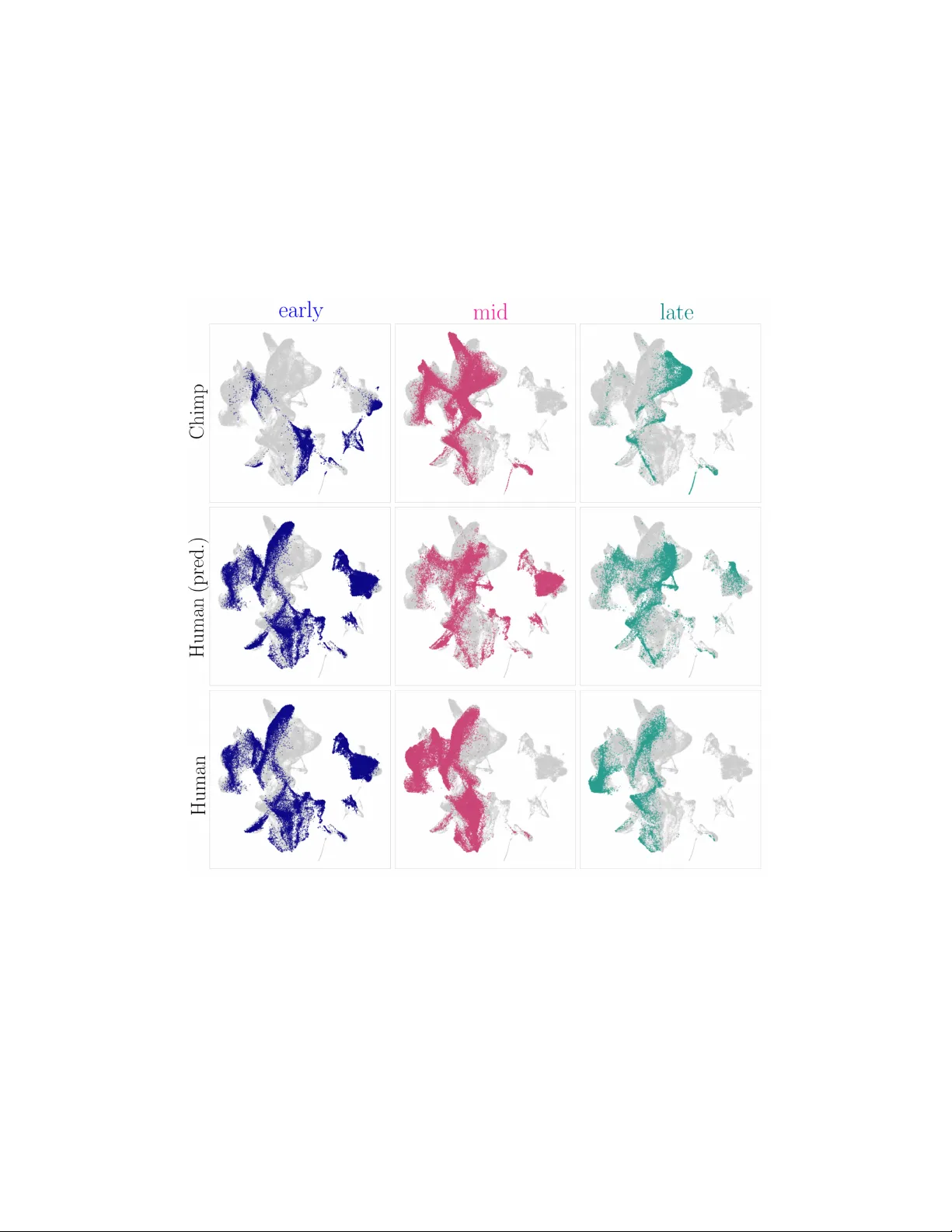
W asserstein P arallel T ransp ort for Predicting the Dynamics of Statistical Systems T ristan Luca Saidi † tsaidi@andrew.cmu.edu Gonzalo Mena † gmena@andrew.cmu.edu Larry W asserman † , ‡ larry@stat.cmu.edu Florian Gunsilius ∗ fgunsil@emory.edu † Departmen t of Statistics and Data Science, Carnegie Mellon Univ ersity ‡ Mac hine Learning Department, Carnegie Mellon Univ ersit y ∗ Departmen t of Economics, Emory Universit y Marc h 26, 2026 Abstract Man y scien tiﬁc systems, suc h as cellular populations or economic cohorts, are naturally describ ed b y probabilit y distributions that ev olve o ver time. Predicting how such a system w ould ha ve ev olv ed under diﬀeren t forces or initial conditions is fundamental to causal inference, domain adaptation, and counterfactual prediction. Ho wev er, the space of distributions often lac ks the v ector space structure on whic h classical metho ds rely . T o address this, w e in tro duce a general notion of parallel dynamics at a distributional lev el. W e base this principle on parallel transp ort of tangent dynamics along optimal transp ort geo desics and call it “W asserstein P arallel T rends”. By replacing the vector subtraction of classic metho ds with geo desic parallel transp ort, w e can pro vide counterfactual comparisons of distributional dynamics in applications such as causal inference, domain adaptation, and batc h-eﬀect correction in experimental settings. The main mathematical contribution is a no vel notion of fanning sc heme on the W asserstein manifold that allo ws us to eﬃciently appro ximate parallel transp ort along geodesics while also providing the ﬁrst theoretical guarantees for parallel transp ort in the W asserstein space. W e also sho w that W asserstein Parallel T rends recov ers the classic parallel trends assumption for a verages as a special case and derive closed-form parallel transport for Gaussian measures. W e deploy the metho d on syn thetic data and tw o single-cell RNA sequencing datasets to impute gene- expression dynamics across biological systems. Con ten ts 1 In tro duction 2 2 Setup and Bac kground 4 2.1 Optimal T ransp ort . . . . . . . . . . . . . . . . . . . . . . . . . . . . . . . . . . . . . 4 2.2 Dynamic F ormulation . . . . . . . . . . . . . . . . . . . . . . . . . . . . . . . . . . . 5 2.3 Riemannian Structure of the W asserstein Space . . . . . . . . . . . . . . . . . . . . . 6 1 3 P arallel T ransp ort 8 3.1 Exact Parallel T ransp ort via the Cov ariant Deriv ativ e. . . . . . . . . . . . . . . . . . 8 3.1.1 Example: W asserstein Parallel T ransp ort with Gaussians . . . . . . . . . . . 9 3.2 Appro ximation via Base P arallel T ransp ort and Jacobi Fields. . . . . . . . . . . . . . 10 3.3 Appro ximate W asserstein Parallel T ransp ort . . . . . . . . . . . . . . . . . . . . . . . 12 3.4 W eighted Helmholtz-Ho dge Decomp osition . . . . . . . . . . . . . . . . . . . . . . . 14 4 Reconstructing Coun terfactual Dynamics 17 4.1 W asserstein Counterfactual Dynamics Prediction . . . . . . . . . . . . . . . . . . . . 17 4.2 Application: Causal Inference via W asserstein Diﬀerence-in-Diﬀerences . . . . . . . . 20 5 Exp erimen ts 22 5.1 Sim ulations . . . . . . . . . . . . . . . . . . . . . . . . . . . . . . . . . . . . . . . . . 22 5.2 Real Data: Genomics . . . . . . . . . . . . . . . . . . . . . . . . . . . . . . . . . . . . 24 6 Conclusion 28 A Stabilit y Theory for W asserstein Parallel T ransp ort 32 A.1 The Stabilit y Theorem . . . . . . . . . . . . . . . . . . . . . . . . . . . . . . . . . . . 35 A.2 Supplementary Results . . . . . . . . . . . . . . . . . . . . . . . . . . . . . . . . . . . 39 B Pro ofs of Results F rom the T ext 52 B.1 Pro of of Theorem 3.3 . . . . . . . . . . . . . . . . . . . . . . . . . . . . . . . . . . . . 52 B.2 Pro of of Theorem 3.11 . . . . . . . . . . . . . . . . . . . . . . . . . . . . . . . . . . . 53 B.3 Pro of of Prop osition 3.13 . . . . . . . . . . . . . . . . . . . . . . . . . . . . . . . . . 54 B.4 Pro of of Lemma 3.8. . . . . . . . . . . . . . . . . . . . . . . . . . . . . . . . . . . . . 55 B.5 Pro of of Theorem 3.9. . . . . . . . . . . . . . . . . . . . . . . . . . . . . . . . . . . . 55 B.6 Pro of of Prop osition 3.7 . . . . . . . . . . . . . . . . . . . . . . . . . . . . . . . . . . 56 B.7 Pro of of Lemma 4.3. . . . . . . . . . . . . . . . . . . . . . . . . . . . . . . . . . . . . 57 B.8 Pro of of Theorem 4.6 . . . . . . . . . . . . . . . . . . . . . . . . . . . . . . . . . . . . 58 B.9 Supplemen tary Results . . . . . . . . . . . . . . . . . . . . . . . . . . . . . . . . . . . 59 C RKHS Deriv ation 61 D Implemen tation Details 63 1 In tro duction Man y scientiﬁc systems are naturally described b y probability distributions that evolv e ov er time, suc h as cellular populations undergoing diﬀeren tiation, income distributions responding to p olicy c hanges, or ecological communities adapting to en vironmen tal shifts. A fundamen tal task is to tak e the dynamics observed for one suc h system and predict how a second system with diﬀerent prop erties w ould hav e evolv ed under similar dynamics. This coun terfactual question sho ws up in sev eral distinct guises; for instance, as causal eﬀect estimation in observ ational studies, as out-of- sample prediction when only one system is observed, and ev en in dynamic randomized treatment estimation as we sho w below. In eac h case, the challenge is the same, namely , to transfer a temporal trend from one distributional baseline to another. Existing approac hes to transferring dynamics rely on taking diﬀerences. In causal inference with observ ational data for instance, Diﬀerence-in-Diﬀerences subtracts the observed c hange in the 2 reference group, relying on the parallel trends assumption ( Abadie , 2005 ; Ashenfelter and Card , 1985 ). Po w erful recent extensions (e.g. Zhou et al. , 2025 ) generalize this to geo desic spaces b y requiring an ab elian group structure, which is needed to deﬁne an analogous notion of “diﬀerence”. W e take a fundamentally diﬀerent approach: rather than computing diﬀerences betw een systems, we dir e ctly tr ansp ort the instantane ous dynamics (the tangent velocity driving the evolution of one system) to the baseline of another via geo desic parallel transp ort on the space of probability mea- sures. This literally constructs a parallel trend. The metho d op erates in con tinuous time and acts on full distributions rather than momen ts. Moreo ver, b ecause the method constructs counterfac- tual tra jectories directly rather than bac king out treatmen t eﬀects from assumed parallelism, it is widely applicable. F or instance, it allo ws for the correction of batc h eﬀects in randomized trials or the imputation of unobserved dynamics when only one system’s dynamics are observed. Our main technical contribution is the in tro duction of a no v el fanning sc heme ( Louis et al. , 2018 ) on the W asserstein manifold that allows us to eﬃcien tly appro ximate parallel transp ort along geo desics while providing the ﬁrst theoretical guarantees for parallel transp ort in the W asserstein space. By lev eraging Jacobi ﬁelds on the base manifold ( Gigli , 2012 ), the sc heme circum ven ts the nonlinear PDE that characterizes exact W asserstein parallel transport ( Am brosio and Gigli , 2008 ). W e further sho w that curves in P 2 ( R d ) that are parallel in the sense of the Levi-Civita connection on the W asserstein manifold necessarily ha ve parallel means, reco vering the classical equibias condition (e.g. Sofer et al. , 2016 ) for av erages as a sp ecial case. W e also derive closed-form expressions for parallel transp ort b et ween Gaussian measures by reducing the problem to a con tin uous Ly apunov equation. Our main application domain is single-cell genomics, where transcriptomic tec hnologies produce snapshots of gene-expression distributions at discrete time p oin ts under v arying biological condi- tions ( Sc hiebinger et al. , 2019 ; Schiebinger , 2021 ; La venan t et al. , 2024 ). Because measuring a cell’s state destro ys it, individual tra jectories are unobserv able, and one m ust reason at the p opulation lev el—a setting where optimal transport has become a standard modeling to ol ( Bunne et al. , 2024 ). A natural use case arises in con trolled p erturbation exp erimen ts, where t w o nominally clonal p op- ulations are cultured in parallel and one receives treatmen t. In man y suc h settings—particularly in vitro systems or carefully designed time-course exp erimen ts—samples from control and treated arms are collected and pro cessed in a co ordinated manner across timepoints, so that technical v ariation is largely shared ov er time. If both p opulations were distributionally identical at base- line, the con trol tra jectory could serve directly as the counterfactual for the treated p opulation. In practice, how ever, even under these controlled conditions, replicates often exhibit systematic baseline diﬀerences, commonly referred to as b atch eﬀe cts , arising from factors such as sample handling or sequencing v ariation ( T ran et al. , 2020 ; Lueck en et al. , 2022 ). In these regimes, it is often reasonable to approximate suc h discrepancies as structured, appro ximately time-in v ariant shifts betw een distributions. Under this assumption, our metho d provides a geometric framew ork for aligning dynamics across baselines: b y parallel transp orting the con trol dynamics along the geo desic connecting the tw o initial distributions, we transfer the observ ed temp oral trend to the treated p opulation while accounting for their initial misalignment. This approach op erates on full distributions rather than lo w-dimensional summaries, capturing diﬀerences b ey ond simple lo cation shifts. Its v alidity , ho wev er, relies on the extent to whic h the baseline discrepancy can b e mean- ingfully represen ted as a stable transformation across time, and is therefore b est suited to settings where time-v arying tec hnical eﬀects or large comp ositional c hanges are limited. Our w ork connects to several strands of literature. The problem of predicting counterfactual dynamics is ubiquitous in causal inference and domain adaptation. In the causal inference litera- ture, Diﬀerence-in-Diﬀerences (DiD) is the most prominen t framew ork for lev eraging parallel trends to estimate treatment eﬀects ( Ashenfelter and Card , 1985 ; Card and Krueger , 1994 ; Abadie , 2005 ; 3 Roth et al. , 2023 ). Distributional extensions hav e been pursued b y Athey and Imbens ( 2006 ), who prop ose univ ariate changes-in-c hanges using monotone transp ort, T orous et al. ( 2024 ), who gener- alize the setting to m ultiv ariate outcomes, and b y Sofer et al. ( 2016 ), who form ulate distributional DiD through quantile transp ort maps. Calla wa y and Li ( 2019 ) introduce parallel trends via a cop- ula stability assumption. Zhou et al. ( 2025 ) extend DiD to geo desic spaces with an ab elian group structure. Other closely related approac hes are distributional extensions of the syn thetic controls metho d ( Abadie et al. , 2010 ; Gunsilius , 2023 ; Gunsilius et al. , 2024 ), whic h also create parallel trends, but via av eraging of p ossible con trol dynamics. Our metho d is applicable to all of these settings but is not limited to causal inference ( Gunsilius , 2025 ): it provides a general-purpose to ol for constructing coun terfactual tra jectories whenev er one wishes to transfer observ ed dynamics to a new distributional baseline. Prior seminal uses of parallel transp ort on the W asserstein manifold are due to Petersen and M ¨ uller ( 2019 ) and Chen et al. ( 2023 ), who emplo y it for F r ´ ec het regression; b oth fo cus on the univ ariate setting and address a fundamentally diﬀeren t problem. Our framew ork can also be view ed as a dynamic coun terpart to optimal transp ort-based domain adaptation ( Courty et al. , 2016 ), which aligns source and target distributions at a single time p oin t; we instead transp ort temp oral dynamics themselv es across distributional baselines. In single-cell genomics, the main application in this paper, Bunne et al. ( 2023 ) use neural optimal transp ort to learn maps from con trol to p erturb ed cell distributions. Their approach is static in that it do es not mo del temp oral dynamics, and learns a direct map b et ween observ ed conditions rather than constructing a counterfactual against which a treatment eﬀect can b e mea- sured. Our framework, by contrast, op erates on evolving distributions ov er time, pro duces explicit coun terfactual tra jectories that enable treatment-con trol comparisons, and provides a testable iden- tifying assumption—W asserstein Parallel T rends—supp orting causal inference from observ ational genomics data alongside pure coun terfactual prediction in exp erimen tal settings. The remainder of the pap er is structured as follows. Section 2 reviews the background on optimal transport and the Riemannian geometry of the W asserstein space. Section 3 dev elops the theory of parallel transp ort on W asserstein space ov er manifolds, introduces the no vel fanning sc heme, and establishes its theoretical guarantees. Section 4 presents the coun terfactual dynamics prediction pro cedure, introduces the W asserstein Parallel T rends assumption, and sho ws that it reco vers the classical equibias condition. Section 5 contains experiments on syn thetic Gaussian systems and tw o single-cell RNA sequencing datasets. All pro ofs are collected in the app endix. 2 Setup and Bac kground In this section we giv e an o verview on the mathematical underpinnings of optimal transp ort and Riemannian geometry as they pertain to our goals. F or a fully detailed treatmen t of the theory of optimal transp ort, we recommend Villani et al. ( 2009 ). F or a comprehensiv e treatmen t of Riemannian and diﬀerential geometry , w e recommend either Lee ( 2018 ) or Petersen ( 2006 ), and Do Carmo ( 2016 ). The Riemannian p ersp ectiv e on optimal transport that w e describe in this section follo ws closely the constructions described by Otto ( 2001 ), Gigli ( 2012 ) and Lott ( 2008 ), and later expanded on b y Clancy ( 2021 ). 2.1 Optimal T ransp ort Deﬁne P 2 ( M ) to b e the set of probabilit y measures with ﬁnite second moment o ver a complete, connected and C ∞ Riemannian manifold M with metric tensor g . F or the sake of generality and applicabilit y to concurrent work, w e will take M to b e a Riemannian manifold satisfying the 4 prop erties described abov e, but all of our algorithmic instantiations and experiments will consider M = R d . The 2-W asserstein distance b et ween t wo probabilit y measures µ, ν ∈ P 2 ( M ) is deﬁned by W 2 ( µ, ν ) = inf γ ∈ Γ µ,ν  Z M × M d M ( x, y ) 2 γ ( dx, dy )  1 / 2 (1) where Γ µ,ν denotes the set of couplings of µ and ν . The 2-W asserstein distance (whic h w e will henceforth refer to as the W asserstein distance) is indeed a metric, whic h renders ( P 2 ( M ) , W 2 ) a metric space. A key result is that of Brenier, who show ed that for M = R d , the optimal coupling tak es the form ( X , ∇ ϕ ( X )) , X ∼ µ for some conv ex ϕ when µ is absolutely contin uous with resp ect to the Leb esgue measure. Theorem 2.1 (Brenier) . L et µ, ν ∈ P 2 ( R d ) b e pr ob ability me asur es such that µ has a density, and let X ∼ µ . If γ ∗ is optimal for Equation (1) with M = R d , then ther e exists a c onvex function ϕ : R d → R such that ( X , ∇ ϕ ( X )) ∼ γ ∗ . This theorem guarantees that if the source measure has a density , then the optimal transp ort coupling can b e written as the source measure µ and ∇ ϕ # µ , the pushforw ard of the source under some con vex function – note that the pushforward of a measure µ under a map T is simply the measure ( T # µ )( B ) = µ ( T − 1 ( B )) for all measurable B . The function ∇ ϕ from Theorem 2.1 is often referred to as the Br enier map . This key theorem of Brenier will b e cen tral to our construction of the Riemannian structure on the space of probabilit y measures. W e note that Brenier’s theorem w as later generalized to Riemannian manifolds, as described b elo w. The result requires generalizing the notion of conv exity and conca vit y to non-Euclidean settings. In particular, giv en a function ψ : M → R ∪ {±∞} its inﬁmal c onvolution ψ c with a cost function c is deﬁned by ψ c ( y ) = inf x ∈ M { c ( x, y ) − ψ ( x ) } . W e say ψ is c -concav e if and only if ψ cc = ( ψ c ) c = ψ . Theorem 2.2 (Brenier-McCann, McCann ( 2001 )) . L et ( M , g ) b e a c omplete R iemannian manifold and let µ, ν ∈ P 2 ( M ) with µ ≪ vol g . Then ther e exists a c -c onc ave function ϕ : M → R with c ( x, y ) = d M ( x, y ) 2 such that the optimal plan (in the sense of Equation (1) ) is induc e d by a µ -a.e. unique map T ( x ) = exp x ( −∇ ϕ ( x )) , γ ∗ = ( id , T ) # µ wher e ∇ is the Riemannian gr adient and exp p ( v ) is the R iemannian exp onential map. 2.2 Dynamic F orm ulation The optimal transp ort problem described abov e – one which lo oks for an optimal coupling of source and target measures – is often referred to as the static formulation of optimal transp ort. An equiv alent p erspective comes from ﬂuid mec hanics, which arrives at the same metric structure through a diﬀerent formulation. In particular, let ( v t ) t ≥ 0 b e a time dep enden t family of v ector ﬁelds ov er M , and consider the ODE ˙ X t = v t ( X t ). Let µ t denote the la w of X t , where X 0 ∼ µ 0 and X t ev olves according to the ODE describ ed previously . Then, the dynamics of µ t ob ey the so-called c ontinuity e quation , ∂ t µ t + div g ( µ t v t ) = 0 (2) in the weak (or distributional) sense, where div g is the Riemannian divergence. 5 Deﬁnition 2.3 (W eak solutions to Equation (2) , Santam brogio ( 2015 )) . We say that a family of p airs ( µ t , v t ) solves the c ontinuity e quation on (0 , T ) in the distributional sense if for any b ounde d and Lipschitz test function ϕ ∈ C 1 c ((0 , T ) × M ) we have Z T 0 Z M ∂ t ϕ dµ t dt + Z T 0 Z M ⟨∇ ϕ, v t ⟩ g dµ t dt = 0 . It turns out, one can iden tify optimal transport maps with v ector ﬁelds satisfying the con tinuit y equation that are optimal in a certain sense. This gives rise to the dynamic form ulation of optimal transp ort. Theorem 2.4 (Benamou-Brenier, Chewi et al. ( 2024 ); Am brosio and Gigli ( 2012 )) . L et µ 0 , µ 1 ∈ P 2 ( M ) b e absolutely c ontinuous with r esp e ct to vol g . Then W 2 2 ( µ 0 , µ 1 ) = inf ( Z 1 0 ∥ v t ∥ 2 L 2 ( µ t ) dt      ( µ t , v t ) t ∈ [0 , 1] satisﬁes Deﬁnition 2.3 ) . Mor e over, if M = R d then the optimal curve ( µ t ) t ≥ 0 is unique and is describ e d by X t ∼ µ t , wher e X t = (1 − t ) X 0 + tX 1 and ( X 0 , X 1 ) ∼ γ ∗ ∈ Γ µ 0 ,µ 1 with γ ∗ b eing an optimal c oupling. 2.3 Riemannian Structure of the W asserstein Space The T angen t Space. The dynamic form ulation of optimal transp ort will b e a key ingredien t in establishing the Riemannian structure of ( P 2 ( M ) , W 2 ). In particular, we will construct the tangent space from the space of solutions to the con tinuit y equation, as they represent the vector space of inﬁnitesimal p erturbations to a measure. But seeing as there are an inﬁnite n umber of solutions to the con tinuit y equation, (as adding a div ergence free ﬁeld do es not change the marginal b eha vior of µ t ) w e need to establish a selection principle. T o do so, we will deﬁne a notion of a “deriv ativ e” in a general metric space. Deﬁnition 2.5 (Metric Deriv ative) . L et ( X , d ) b e a metric sp ac e and ( x t ) t ≥ 0 b e a curve in X . The metric derivative of the curve at time t is given by | ˙ x | ( t ) ≜ lim s → t d ( x s , x t ) | s − t | pr ovide d that the limit exists. No w, for a pair of probability measures µ, ν ∈ P 2 ( M ) where µ admits a density , we will write T µ → ν for the Brenier (or Brenier-McCann) map from µ to ν and we will write | ˙ µ | for the metric deriv ative of a curv e in P 2 ( M ) with respect to the W asserstein metric. Theorem 2.6 ( Am brosio et al. ( 2005 )) . L et ( M , g ) b e a smo oth and c omplete R iemannian manifold without b oundary and let ( µ t ) t ≥ 0 b e an absolutely c ontinuous curve, i.e. µ t admits a Riemannian density and | ˙ µ t | exists for al l t ≥ 0 . Then for every family of ve ctor ﬁelds ( v t ) t ≥ 0 for which Equation (2) holds, it holds that | ˙ µ t | ( t ) ≤ ∥ v t ∥ L 2 ( µ t ) for al l t ≥ 0 . Mor e over, ther e exists a unique family ( v t ) t ≥ 0 such that Equation (2) holds and for which | ˙ µ t | ( t ) = ∥ v t ∥ L 2 ( µ t ) for every t ≥ 0 . This family is such that v t = lim h → 0 +  h − 1 log x ( T µ t → µ t + h ( x ))  in L 2 ( µ t ) and v t = min n ∥ ˜ v t ∥ 2 L 2 ( µ t )    ∂ t µ t + div g ( ˜ v t µ t ) = 0 o wher e log is the Riemannian lo garithmic map. 6 Note that result coupled with Brenier’s theorem indicates that the v elo cit y ﬁeld that coincides (in an L 2 ( µ t ) sense) with the minimal norm solution and the metric deriv ative of the path is a limit of gradients. This key fact giv es rise to the deﬁnition of the tangent space and the metric tensor for ( P 2 ( M ) , W 2 ) at a measure µ . Deﬁnition 2.7 (W asserstein T angent Space, Ambrosio and Gigli ( 2012 )) . L et µ ∈ P 2 ( M ) . We deﬁne the tangent sp ac e to P 2 ( M ) at µ to b e T µ P 2 ( M ) = {∇ ϕ | ϕ ∈ C ∞ c ( M ) } L 2 ( µ ) (3) wher e {·} L 2 ( µ ) denotes the L 2 ( µ ) closur e and C ∞ c denotes the set of c omp actly supp orte d and smo oth maps. We also endow T µ P 2 ( M ) with the metric tensor ⟨∇ ϕ 1 , ∇ ϕ 2 ⟩ µ ≜ Z M ⟨∇ ϕ 1 , ∇ ϕ 2 ⟩ g dµ (4) wher e ⟨· , ·⟩ g is the inner pr o duct deﬁne d by the metric tensor g . The Co v ariant Deriv ative. On an abstract manifold ( M , g ) that isn’t embedded in an am bient space, we hav e no ob vious w ay to compare v ectors in the tangen t space at t wo points p, q ∈ M , p  = q . Therefore, we need a w a y of connecting the separate vector spaces T p M and T q M . One can achiev e this b y deﬁning a rule ∇ for diﬀerentiating v ector ﬁelds against eac h other on M in a w ay that preserv es the structure of the metric g . Note that we will adopt the standard notation that a vector ﬁeld X o ver M is an op erator on functions – in particular, for some f : M → R , the notation X ( f ) denotes the deriv ativ e of f in the direction describ ed by X . Deﬁnition 2.8 (The Cov arian t Deriv ative, P etersen ( 2006 )) . F or a manifold ( M , g ) we deﬁne the c ovariant derivative ∇ to b e a rule that assigns to e ach p air of ve ctor ﬁelds X , Y over M another ve ctor ﬁeld ∇ X Y satisfying 1. Line arity: ∇ aX + bZ Y = a ∇ X Y + b ∇ Z Y . 2. L eibniz/derivation pr op erty: for f ∈ C ∞ ( M ) we have ∇ X ( f Y ) = X ( f ) Y + f ∇ X Y , wher e X ( f ) = g ( X , ∇ f ) is the derivative of f in the dir e ction X . While this giv es us a wa y to connect tangent spaces, the co v ariant deriv ativ e might distort the geometry induced by the metric g – i.e. it migh t not b e “metric compatible”. A fundamen tal result of Riemannian geometry , how ever, is that for an y Riemannian manifold ( M , g ) there exists a unique connection that is torsion free and is “metric compatible”. Theorem 2.9 (The F undamental Theorem of Riemannian Geometry , Petersen ( 2006 )) . If M is a ﬁnite dimensional manifold endowe d with a Riemannian metric g , then ther e exists a unique c onne ction ∇ c al le d the L evi-Civita c onne ction that is 1. T orsion fr e e: ∇ X Y − ∇ Y X = [ X, Y ] , wher e [ X , Y ]( f ) = X ( Y ( f )) − Y ( X ( f )) is the Lie br acket of X and Y . 2. Metric c omp atible: X g ( Y , Z ) = g ( ∇ X Y , Z ) + g ( Y , ∇ X Z ) . In the case of ( P 2 ( M , W 2 ) we can explicitly construct the cov ariant deriv ative, but one needs to man ually verify that it is torsion free and metric compatible, as the space is an inﬁnite-dimensional Riemannian Manifold. 7 Prop osition 2.10 (W asserstein Co v ariant Deriv ative, Clancy ( 2021 ); Gigli ( 2012 )) . L et ( µ t ) t ≥ 0 b e a curve thr ough P 2 ( M ) with tangent ﬁeld ∇ ϕ t solving Equation (2) , and ther efor e driving the dynamics of µ t . Also let v t b e another ve ctor ﬁeld along µ t and let Π µ t b e the ortho gonal pr oje ction onto T µ t P 2 ( M ) in L 2 ( µ t ) . Then the diﬀer ential op er ator ∇ W 2 ( ∇ φ t ) given by ∇ W 2 ( ∇ φ t ) v t = Π µ t  ∂ t v t + ∇ M ( ∇ φ t ) v t  is a valid c ovariant derivative, is torsion fr e e, and is metric c omp atible, wher e ∇ M ( ∇ φ t ) is the L evi- Civita c onne ction on M . Mor e over, when M = R d , we have ∇ W 2 ( ∇ φ t ) v t = Π µ t ( ∂ t v t + ∇ v t · ∇ ϕ t ) . This result establishes a closed form PDE describing a diﬀeren tial operator with the desired c haracteristics of the Levi-Civita connection. W e remark that Π µ t : L 2 ( µ t ; M ) → T µ t P 2 ( M ) is the orthogonal pro jection from the space of L 2 ( µ t ; R d ) vector ﬁelds o ver M to the closure of L 2 ( µ t ; R d ) gr adient ﬁelds ov er M . In practice, this op eration amounts to a (Helmholtz-Ho dge) decomp osition v t = ∇ ϕ t + w t where w t is the (weigh ted) divergence-free comp onen t of the vector ﬁeld v t . W e discuss estimation of this Helmholtz-Ho dge decomp osition in Section 3.4 . The Exp onen tial and Logarithmic Maps. F or P 2 ( M ), the W asserstein exp onen tial map is deﬁned to b e exp µ ( u ) ≜ (exp( u )) # µ where exp( · ) is the exp onen tial map of M and u ∈ L 2 ( µ ; R d ). In the case of M = R d , this op eration is trivial – w e hav e exp µ ( u ) = (id + u ) # µ (5) where id is the identit y map, x 7→ x . In the case of the logarithmic map, things are analogous. W e deﬁne the W asserstein logarithmic map to b e ( log µ ν )( x ) ≜ log x ( T µ → ν ( x )) where T µ → ν is the Brenier map from µ to ν . Again, when M = R d this reduces to ( log µ ν )( x ) = ( T µ → ν − id)( x ) . (6) 3 P arallel T ransp ort Ha ving laid the groundwork of W asserstein geometry , w e will now mo ve on to discussing parallel transp ort in detail. In the ﬁrst part of this section we will describ e the c haracterization of parallel transp ort via the cov ariant deriv ativ e. In the latter parts of this section, we will discuss a fully general appro ximation sc heme for parallel transp ort on P 2 ( M ) along w ell behav ed W asserstein geo desics that uses Jacobi ﬁelds to a void the PDE obtained from the co v ariant deriv ative. 3.1 Exact P arallel T ransp ort via the Co v ariant Deriv ative. In tuitively , a vector ﬁeld along a curve is “unc hanging” if its deriv ativ e is zero. In the con text of abstract manifolds, parallel transp ort is deﬁned based on this principle: a v ector ﬁeld along a curve is the parallel transp ort of a source v ector if its cov ariant deriv ativ e along the curve is zero. Deﬁnition 3.1 ( Lee ( 2018 )) . L et M b e a smo oth Riemannian manifold. A smo oth ve ctor ﬁeld X along a smo oth curve γ is said to b e p ar al lel along γ with r esp e ct to the L evi-Civita c onne ction if ∇ ˙ γ X ≡ 0 . 8 This c haracterization no w allo ws us to deﬁne parallel transp ort on ( P 2 ( M ) , W 2 ) using the co v arian t deriv ative describ ed in Prop osition 2.10 . Consider a smooth curve µ t through P 2 ( M ) indexed by t ∈ (0 , 1) with the tangent ﬁeld ∇ ϕ t driving its dynamics. Then w e hav e the follo wing deﬁnition. Prop osition 3.2 (W asserstein Parallel T ransp ort PDE) . A ve ctor ﬁeld v t along µ t is p ar al lel along µ t with r esp e ct to ∇ W 2 ( ∇ φ t ) if div g  µ t  ∂ t v t + ∇ M ( ∇ φ t ) v t  = 0 for a.e. t ∈ (0 , 1) . Pr o of. Due to Deﬁnition 3.1 and Proposition 2.10 we know that v t is a parallel v ector ﬁeld along the curv e µ t if Π µ t  ∂ t v t + ∇ M ( ∇ φ t ) v t  = 0 for almost every t ∈ (0 , 1) . This is tan tamount to the requiremen t that div g  µ t ( ∂ t v t + ∇ M ( ∇ φ t ) v t )  = 0 since the L 2 ( µ t ) pro jection simply discards the div ergence free p ortion of the vector ﬁeld. This can b e seen b y the fact that the orthogonal complemen t of the tangen t space at a measure µ t is T ⊥ µ t P 2 ( M ) =  w ∈ L 2 ( µ t )   div g ( w µ t ) = 0  as stated in deﬁnition 1.29 of Gigli ( 2012 ). Th us, Π µ t ( w ) = 0 ⇐ ⇒ div g ( µ t w ) = 0. While Prop osition 3.2 describes parallel transp ort along an y curve, solving this PDE in practice ma y b e challenging, esp ecially in high-dimensional settings. T o this end, in the next section we will describ e an alternativ e appro ximate but tractable approach for computing parallel transp ort along ge o desics – our approach leverages the connection b et ween parallel transp ort on the base space M and parallel transp ort on P 2 ( M ) for any Riemannian manifold M (as established b y Gigli ( 2012 )) to enable parallel transp ort on P 2 ( M ). Since computing parallel transport on M is not alw a ys feasible, we also describ e a “fanning” scheme in which one can use Jac obi ﬁelds to approximate the underlying parallel transp ort on M . But b efore doing that, we will derive and analyze W asserstein parallel transp ort on Gaussians to develop some intuition. 3.1.1 Example: W asserstein P arallel T ransport with Gaussians T o build up intuition for the b eha vior of W asserstein parallel transp ort, we will explore the setting where all measures are Gaussian and M = R d . F ortunately , as is often the case, our ob ject of interest is a v ailable in closed form when dealing with Gaussian measures. This closed form expression for parallel transp ort with Gaussian measures is detailed in Theorem 3.3 . W e provide the proof of Theorem 3.3 in Section B.1 . Theorem 3.3 (P arallel T ransp ort along Gaussian Geo desics) . L et µ 0 , µ 1 b e two Gaussian pr ob a- bility me asur es p ar ameterize d by me ans m 0 , m 1 and c ovarianc es Σ 0 , Σ 1 . F urther let v 0 ( x ) = a 0 + A 0 ( x − m 0 ) ∈ T µ 0 P 2 ( R d ) , A 0 ∈ S d b e a tangent ve ctor to µ 0 . Then the p ar al lel tangent ﬁeld v t along µ t with initial c ondition v 0 is given by v t ( x ) = a 0 + A t ( x − m t ) with A t = A 0 + Z t 0 ˙ A s ds wher e m t = (1 − t ) m 0 + tm 1 , and ˙ A t solves the c ontinuous Lyapunov e quation ˙ A t Q t + Q t ˙ A t = S ⊤ t A t Q t + Q t A t S t 9 with Q t = M −⊤ t Σ − 1 0 M − 1 t , M t = (1 − t ) I d + tB , S t = ( I d − B ) M − 1 t and B = Σ − 1 / 2 0  Σ 1 / 2 0 Σ 1 Σ 1 / 2 0  1 / 2 Σ − 1 / 2 0 . F or further in tuition, Figure 1 instan tiates the result presented in Theorem 3.3 . The ﬁgure illustrates how parallel transp orting a tangent v ector v ∈ T ν i P 2 ( R 2 ) along the geodesic betw een ν i and µ ∗ i c hanges its b eha vior when used to push forw ard the measures ν i and µ ∗ i resp ectiv ely . In particular, w e see the tw o w a ys in which Gaussian parallel transp ort preserves the nature of the deformation of the measures – the left hand panel depicts how it preserv es deformation to the co v ariance, while the right hand panel depicts how it preserves changes to the mean. Figure 1: Visualizations of W asserstein Parallel T ransp ort with Gaussian measures in R 2 . The left panel illustrates ho w parallel transp ort captures deformations to the co v ariance, while the right panel illustrates how it captures changes in the mean. 3.2 Appro ximation via Base P arallel T ransp ort and Jacobi Fields. When dealing with non-Gaussian measures, expressions for W asserstein parallel transp ort are not a v ailable in closed form. T o this end, we will describe a fully general procedure that allows one to appro ximate parallel transp ort along geo desics on P 2 ( M ) for any smooth, complete and con- nected Riemannian manifold M . T o do this we will lev erage t w o k ey results: the ﬁrst is the fact that W asserstein parallel transp ort of a tangen t ﬁeld v can b e lo c al ly approximated by the parallel transp ort of the tangen t ﬁeld on the b ase space M along the Lagrangian paths induced by the optimal transport map asso ciated with the geodesic ( Gigli ( 2012 ), Equation 4.18). T o giv e some in tuition for this phenomenon, w e pro vide an illustration in Figure 2 . The second k ey result will b e the fact that parallel transp ort on the b ase space M can also b e locally approximated by a sp eciﬁc Jacobi ﬁeld ( Louis et al. ( 2018 )) – on many Riemannian manifolds, parallel transp ort is not 10 PT exp º ( r ' ) ( v ) º ¹ M P 2 ( M ) v v PT exp( r ' ) ( v ) º exp( r ' ) exp º ( r ' ) ¹ Figure 2: Visualization of appr oximate W asserstein parallel transp ort, where the approximate tangen t vector is giv en by the map p 7→ PT exp p ( ∇ φ ( p )) ( v ( p )) (left), and exact W asserstein parallel transp ort, where the true tangent v ector is given b y the map p 7→ (PT exp ν ( ∇ φ ) ( v ))( p ) (righ t). a v ailable in closed form, but w e may ha ve access to imp ortan t ob jects lik e the Riemann curv ature tensor, the cov ariant deriv ative and the geo desic equations. In settings like this, one can use the Jacobi ﬁeld to approximate parallel transp ort. Although our exp erimen ts in this work consider the case where M = R d , in a concurren t work that dev elops the theory of parallel transport on the space of general p ositive measures o ver R d w e require a non-Euclidean choice of M . Jacobi Fields. Jacobi ﬁelds allow us to measure the eﬀect of curv ature on a one parameter family of geodesics. A Jac obi ﬁeld is a v ector ﬁeld along a geo desic γ capturing the diﬀerence betw een a geo desic and a p erturb ed geo desic along the parameter of the family . Concretely , let γ τ b e a smo oth, one-parameter family of geo desics with γ 0 = γ . Then J ( s ) = ∂ ∂ τ γ τ ( s )     τ =0 ∈ T γ ( s ) M (7) is a Jacobi ﬁeld, and it describ es the inﬁnitesimal b eha vior of the geo desic family ab out τ = 0. Jacobi ﬁelds satisfy the so-called Jacobi equation ∇ ˙ γ ∇ ˙ γ J ( s ) + R ( J ( s ) , ˙ γ ( s )) ˙ γ ( s ) = 0 (8) where ∇ is the cov arian t deriv ative (typically with resp ect to the Levi-Civita connection) ˙ γ ( s ) = dγ ( s ) /ds , and R ( · , · ) is the Riemann curv ature tensor. In diﬀeren tial geometry , the curv ature tensor of a Riemannian manifold M with a connection ∇ measures the noncommutativit y of the cov ariant deriv ative, and is deﬁned as R ( X , Y ) Z = ∇ X ∇ Y Z − ∇ Y ∇ X Z − ∇ [ X,Y ] Z where X, Y , Z ∈ X ( M ) are v ector ﬁelds o ver the manifold. A k ey fact about Jacobi ﬁelds is the follo wing, which arises from the prop erties of the second-order ODE ab o ve. 11 Prop osition 3.4 (Existence and Uniqueness of Jacobi Fields, Prop osition 10.2 of Lee ( 2018 )) . L et γ p ( s ) = exp p ( su ) b e a ge o desic thr ough a Riemannian or pseudo-R iemannian manifold M for some u ∈ T p M . Then for every p air of ve ctors v, w ∈ T p M ther e is a unique Jac obi ﬁeld denote d j p,u ( v , w )( s ) along γ p ( s ) satisfying the initial c onditions j p,u ( v , w )(0) = v and ∇ ˙ γ p j p,u ( v , w )(0) = w . Observ e that this result indicates that one can also deﬁne Jacobi ﬁelds along a geo desic b y solely sp ecifying its zero and ﬁrst order initial conditions. Henceforth, w e will denote with J a Jacobi ﬁeld deﬁned b y a v ariation through geo desics, while w e will denote with j a Jacobi ﬁeld deﬁned through initial conditions. With this in mind, w e will sho w that a particular Jacobi ﬁeld along M can b e used to appro ximate parallel transp ort on M . Prop osition 3.5 (F anning Sc heme, Prop osition B.3 of Louis et al. ( 2018 )) . L et Ω ⊆ M b e a c omp act subset of M with inje ctivity r adius lower b ounde d by η , and let γ p ( s ) = exp p ( su ) b e a ge o desic thr ough ( M , g ) with γ p ([0 , s ]) ⊂ Ω . F urther denote PT M 0 → s ( v ) as the p ar al lel tr ansp ort of v ∈ T p M fr om p = γ p (0) to γ p ( s ) . Then ther e exists an A ≥ 0 such that for al l s < η ∥ u ∥ g we have   s − 1 j p,u (0 , v )( s ) − PT M 0 → s ( v )   g ≤ As 2 ∥ v ∥ g . W e will leverage this result to approximate parallel transp ort on P 2 ( M ) by using parallel trans- p ort on M and a result from Gigli ( 2012 ) that guarantees that parallel transp ort on M and P 2 ( M ) along r e gular curves are in timately linked. 3.3 Appro ximate W asserstein Parallel T ransp ort T o appro ximate P 2 ( M ) parallel transp ort we will use the fanning sc heme described in Prop osi- tion 3.5 and the connection betw een M parallel transp ort and P 2 ( M ) parallel transport along regular curves established by Gigli. Before we describ e our approximation sc heme, we need to rigorously establish when W asserstein parallel transp ort exists. Deﬁnition 3.6 (Regular Curv es, Gigli ( 2012 )) . L et ( µ t ) t ∈ [0 , 1] b e an absolutely c ontinuous curve. We say that ( µ t ) is r e gular if its velo city ve ctor ﬁeld ( v t ) satisﬁes Z 1 0 ∥ v t ∥ 2 L 2 ( µ t ) dt < ∞ and Z 1 0 Lip( v t ) dt < ∞ wher e Lip( v t ) denotes the sp atial Lipschitz c onstant of the ﬁeld v t . Mor e over, we say that ( µ t ) is str ongly r e gular if Z 1 0 ∥ v t ∥ 2 L 2 ( µ t ) dt < ∞ and sup t ∈ [0 , 1] Lip( v t ) < ∞ . Gigli’s notion of regularit y on curv es of measures is a v ery imp ortan t one. In particular, W asser- stein parallel transp ort is only well deﬁned along these regular curves. Along non-r e gular curves of measures, the tangent space do es not v ary smoothly , and therefore parallel transp ort cannot exist. Thus, for the remainder of this pap er, we will consider curves of measures that are regular in the sense describ ed in Deﬁnition 3.6 . F ortunately , when M = R d , standard assumptions on the densities of the source and target measures guarantee this regularity . Prop osition 3.7 (Existence of W asserstein parallel transport, M = R d ) . Assume that for the p air of me asur es ( µ , ν ), their supp orts Ω , Ω ∗ ⊂ R d ar e b ounde d and mutual ly uniformly c onvex domains 12 with r esp e ct to e ach other and have C 4 b oundaries. Also assume that their L eb esgue densities f ∈ C 2 (Ω) and g ∈ C 2 (Ω ∗ ) satisfy λ ≤ f ≤ Λ ∀ x ∈ Ω and λ ≤ g ≤ Λ ∀ x ∈ Ω ∗ for some c onstants 0 < λ ≤ Λ < ∞ . Then, the quadr atic c ost optimal OT map pushing µ to ν , ∇ ϕ , is a glob al ly C 2 diﬀe omorphism and is bi-Lipschitz. F urthermor e, the Wasserstein ge o desic c orr esp onding to ∇ ϕ is r e gular in the sense of Deﬁnition 3.6 , and Wasserstein p ar al lel tr ansp ort ther efor e exists. W e pro vide the pro of of Proposition 3.7 in Section B.6 . This result describ es suﬃcient conditions on the measures that guarantees the needed regularit y for the existence of W asserstein parallel transp ort when M = R d . Note that when M  = R d , w e simply directly assume the needed regularit y of the curv es of measures for parallel transp ort to exist. With this in mind, the follo wing result prop oses an approximation sc heme for parallel transp ort along r e gular ge o desics betw een a source ν and a target µ . Lemma 3.8 (One step appro ximation of P 2 ( M ) P arallel T ransp ort along regular curves) . L et ( M , g ) b e a c omp act R iemannian manifold with inje ctivity r adius b ounde d fr om b elow and supp ose ν ∈ P 2 ( M ) is a me asur e with v ∈ T ν P 2 ( M ) . F urther let µ ∈ P 2 ( M ) b e the tar get me asur e and assume that ther e exists a u such that t 7→ ν t ≜ ( F t ) # ν , t ∈ [0 , 1] (with F t ≜ exp( tu ) ) tr ac es out a str ongly r e gular ge o desic b etwe en ν and µ with velo city ﬁeld ∇ ψ t . Then for s suﬃciently smal l and for w s deﬁne d as w s = Π ν s  s − 1 j ν,u (0 , v ) ( s )  with j ν,u (0 , v ) ( s ) ≜  x 7→ j x,u ( x ) (0 , v ( x )) ( s )  ◦ F − 1 s we have ∥ w s − PT ν → ν s ( v ) ∥ L 2 ( ν s ) ≤ As 2 ∥ v ∥ L 2 ( ν ) +  e R 1 0 Lip( ∇ ψ r ) dr − 1  2 ∥ v ∥ L 2 ( ν )  Z s 0 Lip( ∇ ψ r ) dr  2 . Mor e over, the str ong r e gularity of t 7→ ν t guar ante es that w s appr oximates PT ν → ν s ( v ) , the p ar al lel tr ansp ort of v along the ge o desic exp ν ( tu ) , in the sense that ∥ w s − PT ν → ν s ( v ) ∥ L 2 ( ν s ) ≤ C s 2 for some C > 0 indep endent of s . W e provide the pro of of Lemma 3.8 in Section B.4 . This result allows us to approximate parallel transp ort of a tangent vector v on ( P 2 ( M ) , W 2 ) along str ongly r e gular ge o desics , provided that we are able to solv e for the Jacobi ﬁeld j ν,u on the base space M – in particular, this sc heme appro ximates W asserstein parallel transp ort along an en tire strongly regular geo desic b y dividing it in to a large n umber of small segments, and lo cally parallel transp orting the tangen t ﬁeld along the paths deﬁned b y the optimal transp ort map. Note that if one tak es the base space M = Ω ⊂⊂ R d , the Jacobi ﬁeld appro ximation can be replaced with the exact Euclidean parallel transp ort, which is simply the iden tity map composed with the pullback. In other cases of constan t curv ature, Jacobi ﬁeld solutions are av ailable in closed form. Equipp ed with this general result, we will no w describ e a pro cedure to appro ximate geo desic W asserstein parallel transp ort that ac hieves O ( N − 1 ) accuracy (where N is a user-c hosen appro ximation resolution) detailed in Theorem 3.9 . W e pro vide the pro of in Section B.5 . Theorem 3.9 (Appro ximation of P 2 ( M ) P arallel T ransp ort along strongly regular curves) . Con- sider the setting of L emma 3.8 , wher e ν and µ ar e c onne cte d by a str ongly r e gular ge o desic and 13 deﬁne the appr oximate p ar al lel tr ansp ort map c PT s 1 → s 2 to b e the one describ e d by the pr o c e dur e of L emma 3.8 . Fix some n ∈ N , let s = 1 / N , deﬁne the maps c PT k ≜ c PT ( k − 1) s → k s and PT k ≜ PT ( k − 1) s → k s and let v k = (PT k ◦ · · · ◦ PT 1 )( v ) and ˆ v k = ( c PT k ◦ · · · ◦ c PT 1 )( v ) . Then we have ∥ ˆ v N − v N ∥ L 2 ( µ ) = O ( N − 1 ) . Algorithm 1 Approximate W asserstein Parallel T ransp ort (WPT) Require: Abs. con tinuous ν , µ ∈ P 2 ( M ), tangent v ector v ∈ T ν P 2 ( M ), discretization lev el N . 1: Compute the Brenier map T ν → µ . 2: Set u ( x ) = log x ( T ν → µ ( x )) and s = 1 / N .  u generates the geo desic 3: for i = 0 , . . . , N do 4: F i ( x ) = exp x  isu ( x )  . 5: v 0 = v .  initialize transp orted ﬁeld 6: for i = 1 to N do 7: ν i = ( F i ) # ν , S i = F i ◦ F − 1 i − 1 , u i ( x ) = log x ( S i ( x )).  one-step transp ort 8: w i ( x ) = s − 1 j ( x,u i ( x )) (0 , v i − 1 ( x ))( s ).  Jacobi propagation on M 9: v i = Π ν i ( w i ◦ S − 1 i ).  pro ject to T ν i P 2 ( M ) 10: return v N ∈ T µ P 2 ( M ). 3.4 W eighted Helmholtz-Ho dge Decomp osition The L 2 ( µ ) pro jection of velocity ﬁelds required in Algorithm 1 is a non-trivial computational pro cedure, and it w arrants further discussion. In this section w e will propose a pro cedure for estimating this v ector ﬁeld pro jection using R epr o ducing Kernel Hilb ert Sp ac e (RKHS) regression. In this section w e will assume that the measure µ has a Leb esgue density ρ . The pro jection Π µ : L 2 ( µ ; R d ) → T µ P 2 ( R d ) maps L 2 ( µ ; R d ) v ector ﬁelds to the L 2 ( µ ) closure of gradien t ﬁelds through the following optimization pro cedure,: Π µ ( v ) = arg min u ∈G µ ∥ u − v ∥ 2 L 2 ( µ ) where G µ ≜ {∇ φ : φ ∈ C ∞ c ( R d ) } L 2 ( µ ) . T o estimate this pro jection from samples, we will use Repro ducing Kernel Hilb ert Space (RKHS) regression. A Repro ducing Kernel Hilb ert Space (RKHS) is a Hilb ert space H of functions f : X → R with a so-called r epr o ducing kernel K : X × X → R c haracterized b y the property that K ( x, · ) ∈ H and f ( x ) = ⟨ K ( x, · ) , f ⟩ H ( Aronsza jn , 1950 ). A key reason for the widespread adoption of RKHSs in statistical applications is the represen ter theorem, whic h c haracterizes solutions of regression problems when optimizing ov er the function class H sub ject to a norm p enalt y . Theorem 3.10 (Representer Theorem) . F or a dataset X = { x i } n i =1 , c onsider an RKHS H of functions f : X → R with a kernel K . F or the optimization pr oblem f ∗ ∈ arg min f ∈H n X i =1 | f ( x i ) − y i | 2 + λ ∥ f ∥ 2 H 14 the solution c an b e expr esse d as f ∗ = n X i =1 α i K ( x i , · ) for a set of sc alars α 1 , . . . , α n . One can ﬁnd a proof b y Gho jogh et al. ( 2021 ). The result stems from the fact that the optimization problem is a norm-p enalized L 2 ( P n ) pro jection onto the RKHS, and solutions therefore lie in the span of kernel sections K ( x i , · ). The critical implication is that for a ﬁxed dataset { x 1 , . . . , x n } one only needs to solv e for α = ( α 1 , . . . , α n ) ⊤ ∈ R n via α ∗ ∈ arg min α ∈ R n ∥ Y − K α ∥ 2 2 + λα ⊤ K α whic h has the solution α = ( K + λI n ) − 1 Y where K ij = K ( x i , x j ) when K is in vertible. T o adapt this to our setting, where w e instead w ant to ﬁnd the b est gr adient-ﬁeld solution, w e will mak e the follo wing modiﬁcation. Let H b e a scalar RKHS on R d with a t wice-diﬀerentiable Mer c er kernel (see Zhou ( 2008 )) K ∈ C 2 ( R d × R d ) and consider the function class {∇ f : f ∈ H} . F or a p opulation measure µ and target ﬁeld v : R d → R d deﬁne the p opulation-lev el solution f ∗ λ ∈ arg min f ∈H n ∥∇ f ( x ) − v ( x ) ∥ 2 L 2 ( µ ) + λ ∥ f ∥ 2 H o (9) and the sample analogue ˆ f λ ∈ arg min f ∈H ( 1 n n X i =1 ∥∇ f ( x i ) − v ( x i ) ∥ 2 2 + λ ∥ f ∥ 2 H ) . (10) W e then ha ve the follo wing result, which we call the gr adient representer theorem. W e provide the pro of of Theorem 3.11 in Section B.2 . Theorem 3.11 (Gradien t Represen ter Theorem) . The optimization pr oblem in Equation (10) has a solution of the form ˆ f λ ( · ) = P n i =1 ⟨ c i , ∇ K ( x i , · ) ⟩ for some set of ve ctors c i ∈ R d and the inner pr o duct is the standar d Euclide an inner pr o duct on R d . As with classical RKHS regression, we can obtain a closed-form solution for the empirical optimizers c ∗ 1 , . . . , c ∗ n b y solving a linear system. Let D ∈ R nd × nd b e the blo c k matrix where D ij = ∇ 2 2 K ( x i , x j ) ∈ R d × d , let G ∈ R nd × nd b e a blo c k Gram matrix where G ij = ∇ 1 ∇ 2 K ( x i , x j ) ∈ R d × d and deﬁne the stack ed vectors c ≜ ( c 1 , . . . , c n ) ⊤ ∈ R nd and v ≜ ( v ( x 1 ) , . . . , v ( x n )) ⊤ . It follo ws that the RKHS norm of ˆ f can b e written as ∥ ˆ f ∥ 2 H = c ⊤ Gc , and our empirical ob jective function is J ( c ) = 1 n ∥ D c − v ∥ 2 2 + λc ⊤ Gc. If D ⊤ D + nλG is inv ertible, then the ob jectiv e function admits a unique minimizer c ∗ = ( D ⊤ D + nλG ) − 1 D ⊤ v , and our estimated pro jected ﬁeld is giv en by ∇ ˆ f n,λ =    ∇ ˆ f ( x 1 ) . . . ∇ ˆ f ( x n )    = D c. W e pro vide the full deriv ation of the empirical ob jective function J and the solution ∇ ˆ f n,λ in Section C . W e will no w sho w that this pro cedure is consistent for estimating the Helmholtz-Ho dge pro jection. 15 Theorem 3.12. L et Ω ⊂ R d b e c omp act, let µ b e a pr ob ability me asur e supp orte d on Ω , and let v ∈ L 2 ( µ ; R d ) such that ∥ v ( x ) ∥ 2 ≤ M < ∞ for µ -a.e. x . L et H b e a sc alar RKHS on R d with kernel K , and assume: 1. F or e ach j ∈ { 1 , . . . , d } and x ∈ R d , the derivative r epr esenter ψ j exists, ψ j ( x ) ≜ ∂ j K ( x, · ) ∈ H and κ 2 ≜ sup x ∈ R d d X j =1 ∥ ψ j ( x ) ∥ 2 H < ∞ . 2. The RKHS gr adient class is dense in the gr adient subsp ac e, i.e. {∇ f : f ∈ H} L 2 ( µ ) = G µ . Deﬁne ˆ f n,λ ∈ arg min f ∈H ( 1 n n X i =1 ∥∇ f ( x i ) − v ( x i ) ∥ 2 2 + λ ∥ f ∥ 2 H ) wher e x 1 , . . . , x n ∼ µ . Then if λ = O ( n − ℓ ) for any  ∈ (0 , 1 / 2) , we have ∥∇ ˆ f n,λ − Π µ ( v ) ∥ L 2 ( µ ) p − → 0 . Pr o of. Let f ∗ λ b e deﬁned as in Equation (9) . T o pro v e this result w e will lev erage the results of De Vito et al. ( 2005 ), where the consistency that w e desire is prov en for bounded linear op erators A : H → K where K is another Hilb ert space. Under the hypotheses stated, Prop osition B.3 indicates that the op erator A = ∇ is indeed a b ounded linear operator. Theorem 5 of De Vito et al. ( 2005 ) giv es ∥∇ ˆ f λ − P v ∥ L 2 ( µ ) → 0 where P is the orthogonal pro jection on to Ran( A ), which in our case satisﬁes Ran( A ) = {∇ f : f ∈ H} L 2 ( µ ) . Since the space {∇ f : f ∈ H} is assumed to b e dense in {∇ f : f ∈ C ∞ c ( R d ) } L 2 ( µ ) , w e kno w that P v = Π µ ( v ). Theorem 3.12 guaran tees consistency of the RKHS pro cedure under the assumption that the function class is dense in the space of gradients of functions of in terest. W e will no w show that this prop erty is satisﬁed when one chooses a k ernel inducing an RKHS that is norm-equiv alent to a Sob olev space of ﬁnite smo othness. Recall that a Sob olev space W k,p ( R ) for 1 ≤ p ≤ ∞ is the subset of functions f in L p ( R ) suc h that f and its w eak deriv atives up to order k ha ve ﬁnite L p norm. When p = 2, the function space forms a Hilb ert space and we denote H k = W k, 2 . Prop osition 3.13 (Suﬃcien t conditions for densit y) . L et µ b e a me asur e supp orte d on a c omp act domain Ω ⊂ R d . Supp ose that µ admits a L eb esgue density ρ satisfying ρ ≤ M < ∞ , and let K b e a kernel such that H , the RKHS induc e d by K , is set and norm e quivalent (denote d ∼ = ) to the Sob olev sp ac e H τ ( R d ) for some τ ∈ N . Then {∇ f : f ∈ H} L 2 ( µ ) = {∇ f : f ∈ C ∞ c ( R d ) } L 2 ( µ ) . and thus {∇ f : f ∈ H} is dense in {∇ f : f ∈ C ∞ c ( R d ) } L 2 ( µ ) . W e provide the proof of Prop osition 3.13 in Section B.3 . The result indicates that any c hoice of kernel yielding an RKHS that is equiv alen t (as sets and in norm) to the Sobolev space H τ ( R d ) 16 Figure 3: Estimated pro jection of a non-conserv ative vector ﬁeld onto the space of gradien t ﬁelds using the pro cedure describ ed in Section 3.4 for some τ ≥ 1 yields the densit y condition needed for consistency ( Theorem 3.12 ). An example of suc h a k ernel is the M´ atern kernel ( Mat´ ern , 1960 ), K a,p ( x, y ) = 2 1 − p Γ( p )  ∥ x − y ∥ 2 a  K p  ∥ x − y ∥ 2 a  (11) for some a, p > 0 where K p ( · ) is the mo diﬁe d Bessel function of the se c ond kind ( Emery et al. , 2025 ). When one c ho oses this k ernel with p > 0, the k ernel’s sp ectral densit y b K ( ω ) satisﬁes b K ( ω ) ≍ (1 + ∥ ω ∥ 2 2 ) − p − d/ 2 , which makes it norm equiv alent to H p + d/ 2 ( R d ) ( Emery et al. , 2025 ). 4 Reconstructing Counterfactual Dynamics Equipp ed with an algorithm for appro ximating W asserstein parallel transport, we will no w leverage it to construct a procedure for predicting dynamics on the space of measures under a parallel trends assumption. In this section we will explicitly state the algorithm, and we will prov e an error b ound that quantiﬁes the distance b et ween the predicted counterfactual dynamics and the true dynamics; w e note that this error bound represen ts p opulation lev el appr oximation error, and does not include statistical error. W e defer a rigorous treatmen t of the statistical asp ects of estimating parallel transp ort to future work. After describing the algorithm, we will illustrate the conceptual utilit y of this pro cedure by instan tiating it in the Diﬀerence-in-Diﬀerences framework in Causal Inference, and showing that it reco vers the w ell known p ar al lel tr ends assumption. 4.1 W asserstein Coun terfactual Dynamics Prediction Our pro cedure for predicting counterfactual dynamics will follo w that depicted in Figure 4 . In particular, giv en a control curve { ν i } i ∈{ 1 ,...,T } ⊂ P 2 ( M ) and an initial condition µ ∗ 1 , w e will predict { ˆ µ ∗ i } i ∈ [2 ,...,T ] as follows: at a given iteration i we will ﬁrst estimate the tangent velocity driving the dynamics of ν i at the current time. W e will then approximate the parallel transp ort of this tangent v elo cit y on the geo desic b et ween the current ν i and the most recen t prediction ˆ µ ∗ i – note that when i = 1, ˆ µ ∗ 1 is set to the initial condition µ 1 . Finally , w e will push ˆ µ ∗ i through the W asserstein exp onen tial map with the parallel transported v elo cit y . While our theoretical results in previous sections allo wed for non-Euclidean c hoices of M , in this section our error bounds consider the setting M = T d , where T d is the ﬂat torus deﬁned b y 17 r ' 0 r ' 1 c PT( d r ' 0 ) c PT( d r ' 1 ) º 0 º 0 ¹ ¤ 0 ¹ ¤ 0 P 2 ( M ) P 2 ( M ) º 1 ¡ ! ¡ ! : : : º 1 ¹ ¤ 1 º 2 º 2 b ¹ ¤ 1 b ¹ ¤ 1 b ¹ ¤ 2 Figure 4: Visualization of coun terfactual dynamics prediction pro cedure described in Algorithm 2 . T d = R d / Z d . W e restrict our analysis to this setting in analyzing our counterfactual dynamics prediction algorithm as the analysis requires stabilit y b ounds on W asserstein parallel transp ort that are c hallenging to obtain in non-Euclidean settings, and settings where the domain has a b oundary . W e also note that our inten tion with the theoretical results presented in this section are to rigorously quantify how our approximation sc heme aﬀects predicted dynamics aw ay from the b oundary of the supp ort; this goal mak es M = T d a natural c hoice, as it is a b oundaryless, compact and ﬂat space. Assumption 4.1 (Uniform admissibilit y of the tra jectory class, M = T d ) . Ther e exists a class C ⊂ P 2 ( T d ) such that the me asur es app e aring in the pr o c e dur e satisfy ν i , µ ∗ i , ˆ µ ∗ i ∈ C for al l i ∈ { 1 , . . . , T } . Mor e over, we r e quir e the fol lowing: (A.1) Density r e gularity c onditions: A l l me asur es µ ∈ C , and al l p airwise Wasserstein inter- p olants µ t ther e of, admit L eb esgue densities ρ , ρ t such that: (a) ther e exist c onstants 0 < λ ≤ Λ < ∞ such that λ ≤ ρ ≤ Λ and λ ≤ ρ t ≤ Λ . (b) the interp olating densities ar e uniformly b ounde d in a Sob olev sense, i.e. sup t ∈ [0 , 1] ∥ ρ t ∥ W 1 , ∞ ( T d ) ≤ K. (c) the map t 7→ ρ t is absolutely c ontinuous as a map fr om [0 , 1] into L ∞ ( T d ) and the interp olating densities have a uniformly b ounde d time derivative, i.e. sup t ∈ [0 , 1] ∥ ∂ t ρ t ∥ L ∞ ( T d ) ≤ K ρ (d) the interp olating densities have a uniformly b ounde d sc or e function in an L ∞ sense, i.e. sup t ∈ [0 , 1] ∥∇ log ρ t ∥ L ∞ ( T d ) ≤ K log . 18 (A.2) Wasserstein ge o desic Lipschitz c onditions: Al l triplets ( ν, µ, µ ′ ) ∈ C satisfy the fol- lowing: (a) the densities ρ t , ρ ′ t of the Wasserstein interp olants of ( ν, µ ) and ( ν , µ ′ ) satisfy ∥ ρ t − ρ ′ t ∥ L ∞ ( T d ) ≤ C L · W 2 ( µ, µ ′ ) and ∥ ρ t − ρ ′ t ∥ W 1 , ∞ ( T d ) ≤ C W W 2 ( µ, µ ′ ) for some C L , C W > 0 . (b) the tangent velo cities ∇ φ t , ∇ φ ′ t of the Wasserstein interp olants of ( ν, µ ) and ( ν , µ ′ ) satisfy ∥∇ φ t − ∇ φ ′ t ∥ L ∞ ( T d ) ≤ C vel · W 2 ( µ, µ ′ ) . (A.3) Wasserstein ge o desic r e gularity c onditions: A l l p airs ( ν , µ ) ∈ C admit ge o desic inter- p olants µ t with velo city ﬁelds ∇ φ t that ar e uniformly b ounde d in a Sob olev sense sup t ∈ [0 , 1] ∥∇ φ t ∥ W 1 , ∞ ( T d ) ≤ M for some M > 0 . In this section, we will operate under the conditions detailed in Assumption 4.1 . These assump- tions guarantee the existence of strongly regular geodesics (in the sense of Deﬁnition 3.6 ) b et ween all pairs of measures of interest. Moreo ver, the assumptions guaran tee the stability of W asserstein parallel transport needed to obtain error bounds for our dynamics prediction algorithm, Algo- rithm 2 . Theorem 4.2 ( Theorem A.3 , Stability of W asserstein Parallel T ransp ort) . Supp ose al l statements in Assumption 4.1 hold. Then ther e exists a c onstant C WPT > 0 , dep ending only on the c onstants ab ove, such that for every v ∈ T ν P 2 ( T d ) ∩ H 1 ( ν ; R d ) , ∥ PT ν → µ ( v ) − PT ν → µ ′ ( v ) ∥ L 2 ( ν ) ≤ C WPT ∥ v ∥ H 1 ( ν ) W 2 ( µ, µ ′ ) . W e pro vide the pro of of Theorem 4.2 in Section A.1 . This stability result allows us to con trol the error of the iterative dynamics prediction algorithm describ ed in Algorithm 2 by ensuring that small approximation errors in the counterfactual do not cause unbounded growth in the terminal error of the parallel transported tangen t at the approximate counterfactual. Concretely , we use this stability to establish the following one-step error b ound described in Lemma 4.3 . Algorithm 2 Counterfactual dynamics prediction via WPT Require: Suﬃcien tly regular con trol tra jectory ( ν i ) T i =1 , treated initial condition µ 1 ∈ P 2 ( M ), discretization level N . 1: Initialize ˆ µ ∗ 1 ← µ 1 .  starting counterfactual state 2: for i = 1 to T − 1 do 3: Compute T ν i → ν i +1 . 4: Set v ( i ) ( x ) ≜ log x ( T ν i → ν i +1 ( x )).  control velocity 5: ˆ w ( i ) = WPT( ν i , ˆ µ ∗ i , v ( i ) , N ).  Algorithm 1 6: ˆ µ ∗ i +1 = exp ˆ µ ∗ i ( ˆ w ( i ) ).  adv ance coun terfactual state 7: return ( ˆ µ ∗ i ) T i =1 . 19 Lemma 4.3 (One step error of Algorithm 2 , M = T d ) . L et ν i , ν i +1 , µ ∗ i , ˆ µ ∗ i ∈ C , wher e C is the admissible class fr om Assumption 4.1 . Supp ose ther e exists a tangent ve ctor ∇ ϕ i ∈ T ν i P 2 ( T d ) such that exp ν i ( ∇ ϕ i ) = ν i +1 . L et ∇ ϕ ∗ i denote the p ar al lel tr ansp ort of ∇ ϕ i along the str ongly r e gular Wasserstein ge o desic c on- ne cting ν i and µ ∗ i , and deﬁne µ ∗ i +1 ≜ exp µ ∗ i ( ∇ ϕ ∗ i ) . L et ˆ v b e the output of Algorithm 2 use d to pr e dict the next c ounterfactual iter ate ˆ µ ∗ i +1 ≜ exp ˆ µ ∗ i ( ˆ v ) . Then W 2 ( ˆ µ ∗ i +1 , µ ∗ i +1 ) ≤  1 + Lip( ∇ ϕ ∗ i ) + ∥∇ ϕ i ∥ H 1 ( T d ) C WPT  W 2 ( ˆ µ ∗ i , µ ∗ i ) + O ( N − 1 ) . W e provide the pro of of Lemma 4.3 in Section B.7 . The result establishes that each iteration of the pro cedure incurs an O ( N − 1 ) error of the coun terfactual prediction in a W asserstein sense. F ortunately , since N corresp onds to the user chosen appro ximation resolution, the one step error can be made arbitrarily small. W e also ha ve the follo wing corollary , whic h quan tiﬁes the cum ulativ e error ov er the en tire pro cedure. Theorem 4.4. In the r e gime describ e d in Assumption 4.1 we have the fol lowing ac cumulate d err or b ound on the c ounterfactual tr aje ctory, T X i =1 W 2 ( ˆ µ i , µ ∗ i ) = O  T N · (1 + L + S C WPT ) T − 1 L + S C WPT  under the assumption that ∥∇ ϕ i ∥ H 1 ( T d ) ≤ S and Lip( ∇ ϕ ∗ i ) ≤ L for al l i ∈ { 1 , . . . , T − 1 } . In the setting wher e T = Θ(1) and N → ∞ , the ac cumulate d err or is o (1) . Pr o of. The result of Lemma 4.3 implies a recurrence relation of the form a t +1 = ca t + r and a 0 = 0, the solution to which has the form a t = ( r · c t − 1 c − 1 when c  = 1 tr when c = 1 . Plugging in c = 1 + L + S C WPT and r = O ( N − 1 ) yields the time-indexed error. Summing o ver i yields the result. No w we are equipp ed with a consistent metho d for imputing the dynamics of a reference curv e { ν i } i ∈{ 1 ,...,T } on to a new initial condition via W asserstein parallel transp ort. In the follo wing sec- tions, we will discuss and explore applications of this algorithm to v arious settings and datasets. 4.2 Application: Causal Inference via W asserstein Diﬀerence-in-Diﬀerences In this section w e describ e an instantiation of our algorithm in Causal Inference – in particular, we illustrate ho w it can b e used to extend the Diﬀerence-in-Diﬀerences (DiD) framework from scalar to distribution-v alued outcomes. The traditional DiD framew ork is as follows: we observe sub jects at time 0 and time 1 where a treatmen t has b een administered somewhere in b et w een, with the observ ations denoted ( Y 0 , Y 1 ). W e denote Y 0 (0) and Y 1 (0) as the counterfactual outcome, had this sub ject not been treated. While Y i (1) need not b e equal to Y i in general, we will assume that this 20 Time Outcome Pre P ost t 0 Z 1 Y 1 Y 1 (0) P 2 ( M ) ν t µ t µ ∗ t t 0 Figure 5: Diﬀerence-in-diﬀerences diagram illustrating the parallel trends assumption in the Eu- clidean case (left) and the W asserstein case (right). The goal is to reconstruct the counterfactual (denoted Y t (0) on the left and µ ∗ t on the right). is the case – this is commonly referred to as the c onsistency assumption. W e also observ e a control group at the tw o times whose observ ations are denoted ( Z 0 , Z 1 ) . Since the control group is un treated, an y diﬀerence b et w een Z 0 and Z 1 stems from unobserved confounding. A standard assumption in the Diﬀerence-in-Diﬀerences framew ork is the e quibias or the p ar al lel tr ends assumption, which stipulates that E [ Y 1 (0) − Y 0 (0)] = E [ Y 1 − Y 0 ] − E [ Z 1 − Z 0 ] ensuring that the trends in untreated individuals are “parallel” ( Abadie , 2005 ) and allowing us to recov er the treatment eﬀect. Note that this pro cedure t ypically op erates on the lev el of ﬁrst-order moments, and it does not deal with the full counterfactual distribution. In man y cases, w e care about the laws µ t ≜ Law( Y t ) and ν t ≜ Law( Z t ) as opp osed to statis- tics lik e their exp ected v alue, but w e cannot take diﬀerences on P 2 ( M ) to subtract oﬀ diﬀerences in initial conditions. T o remedy this, we will apply W asserstein parallel transp ort. In partic- ular, we consider the setting where the population-level treated, un treated and con trol ob jects can b e represented b y piecewise-geo desic tra jectories through P 2 ( M ). F or a set of observ ation times { t i } i ∈{ 1 ,...,T } ⊂ [0 , 1], we denote ( µ t i ) i ∈{ 1 ,...,T } the path corresp onding to the treated popula- tion, ( ν t i ) i ∈{ 1 ,...,T } the path corresp onding to the untreated p opulation, and ( µ ∗ t i ) i ∈{ 1 ,...,T } the path corresp onding to the coun terfactual treated population. Our goal is to emulate the Diﬀerence-in- Diﬀerences pro cedure and reconstruct the p opulation counterfactual tra jectory ( µ ∗ t i ) i ∈{ 1 ,...,T } giv en the control tra jectories and the initial condition of the treated p opulation µ ∗ t 0 (b efore treatmen t). Assumption 4.5 (W asserstein P arallel T rends) . We assume that the tr aje ctories ( ν t i ) i ∈{ 1 ,...,T } and ( µ ∗ t i ) i ∈{ 1 ,...,T } ar e p ar al lel in the fol lowing sense: for al l i ∈ { 1 , . . . , T − 1 } , the tangent velo city at ν t i given by ∇ ϕ t i ≜ log ν t i ( ν t i +1 ) and the tangent velo city at µ ∗ i given by ∇ ϕ ∗ t i = log µ ∗ t i ( µ ∗ t i +1 ) ar e p ar al lel with r esp e ct to the c onne ction ∇ W 2 in the sense that ∇ ϕ ∗ t i = PT ν t i → µ ∗ t i ( ∇ ϕ t i ) wher e PT ν t i → µ ∗ t i is the p ar al lel tr ansp ort of ∇ ϕ t i along the Wasserstein ge o desic b etwe en ν t i and µ ∗ t i . In order for the coun terfactual tra jectory to be reco verable, w e need an assumption analogous to the parallel trends assumption in Euclidean Diﬀerences-in-Diﬀerences. Since w e are not considering ob jects living in a vector space, w e hav e no notion of taking diﬀerences. Instead w e will use 21 W asserstein parallel transp ort to formulate an analogous assumption. This assumption, which w e call Wasserstein Par al lel T r ends , is described in Assumption 4.5 , and we provide a visualization in Figure 5 . F urthermore, we ha ve the following key result, whic h establishes that when M = R d , parallel curves in W asserstein space hav e p ar al lel me ans to o . Theorem 4.6 (W asserstein Parallel T rends recov ers Parallel T rends in R d ) . Supp ose ( ν t ) t ∈ [0 , 1] and ( µ ∗ t ) t ∈ [0 , 1] ar e curves of absolutely c ontinuous me asur es in P 2 ( R d ) , and supp ose that the curves have tangent velo city ﬁelds ∇ ϕ t , ∇ ϕ ∗ t that ar e p ar al lel with r esp e ct to ∇ W 2 for al l t , in the sense that ∇ ϕ ∗ t = PT ν t → µ ∗ t ( ∇ ϕ t ) ∀ t ∈ [0 , 1] . Then it holds that for a.e. t d dt Z R d x dν t ( x ) = d dt Z R d x dµ ∗ t ( x ) . W e provide the pro of of Theorem 4.6 in Section B.8 . This result ensures that our assumptions reco ver the classical e quibias assumption, while also capturing changes in the global “shap e” of the distribution. W e b eliev e that this result motiv ates the application of W asserstein parallel transp ort and our proposed coun terfactual dynamics pro cedure in Causal inference settings; in particular, augmen ting DiD with W asserstein parallel transport would enable estimation of treatmen t eﬀects that manifest through changes in the shap e of the distribution in addition to changes in the means. 5 Exp erimen ts W e now pivot to demonstrating the utility of our conceptual framework and prop osed algorithms through simulations. W e b egin b y showing simulation results of our appro ximation scheme on syn thetic data, do cumen ted in Section 5.1 . Then, we apply our counterfactual dynamics prediction metho d to t wo single-cell RNA sequencing (scRNAseq) datasets, where we impute the gene-level dynamics of one biological system on to another. W e pro vide these genomics exp erimen ts in Sec- tion 5.2 . F or a detailed treatment of our exact computational implemen tation of appro ximate W asserstein parallel transport ( Algorithm 1 ) and the counterfactual dynamics prediction metho d ( Algorithm 2 ), please see Section D . 5.1 Sim ulations W e b egin by ev aluating our proposed algorithms on synthetic data. In particular, we ev aluate Algorithm 2 on a sto c hastic system of time-evolving Gaussian measures, as in this regime we ha ve access to closed form parallel transp ort expressions (whic h we deriv ed in Section 3.1.1 ). W e explore ho w the dimension d aﬀects the qualit y of the predicted tra jectories as measured b y W asserstein distance, and we compare across metho ds. As mentioned, Figure 6 illustrates an application of Algorithm 2 to a system of Gaussian measures ev olving in parallel. The top ro w consists of a sequence of measures where the mean ev olves in time, while the b ottom row illustrates a sequence where both the mean and the co v ariance ev olves in time. W e displa y the reconstructed parallel curves in warm colors for our metho d ( Algorithm 2 ) and for tw o baselines: the ﬁrst baseline applies the same change in mean as observed in the control tra jectory to the coun terfactual initial condition. The second baseline uses the tra jectory induced by the Brenier map b et ween successiv e time p oin ts on the control curve without using parallel transport. In this setup w e use the ground truth Brenier map b et w een the underlying 22 con trol Gaussian measures as extending the empirical Brenier map out of sample is nontrivial – while this is not a tractable baseline in practice, w e b elieve it to b e illustrativ e. Figure 6 indicates that the cumulativ e error for the system of Gaussians with evolving means and stationary co v ariances grows at a comparable rate for our metho d and the baselines as expected. Since the co v ariances of the sequence of measures is unc hanging, one w ould exp ect that the mean- sensitiv e baseline is successful. Moreo v er, the stationary nature of the co v ariances guarantees that the Brenier map is just a shift; this explains the goo d performance. F or the system with a non- stationary co v ariance, ho wev er, we see a signiﬁcan tly faster growth in the cumulativ e error in the baseline metho ds. The mean-shifted baseline metho d eviden tly do esn’t incorp orate information ab out the change in the shap e of the distribution ov er time, while the Brenier map baseline clearly do esn’t lead to imputed dynamics that are parallel in any desirable sense. (a) Parallel sequences of Gaussian measures with changing means. (b) Parallel sequences of Gaussian measures with changing means and changing cov ariances. Figure 6: Illustration of the parallel transp orted dynamics for t wo systems of time-evolving Gaussian measures using our metho d and tw o baselines. T o get a sense of ho w the p erformance of our metho d dep ends on dimension, we also ev aluate on Gaussian measures for d ∈ { 2 , 4 , 8 , 12 , 16 } . In particular, w e compute the W asserstein distance b et ween the true and predicted pushforward of a parallel transp orted tangent b et w een tw o random Gaussian measures. W e rep ort the results of our metho d, the mean-shift baseline and the (non parallel transp orted) Brenier map baseline as a function of dimension in T able 1 . In this table w e add an “estimated” Gaussian baseline (labeled “Gauss PT”), which estimates the parameters of a Gaussian and then applies closed form Gaussian parallel transp ort ( Theorem 3.3 ). W e wish to highligh t tw o key tak eaw a ys from this exp erimen t – ﬁrstly , w e see that our metho d without the Helmholtz pro jection consisten tly outp erforms all other metho ds (except the estimated Gaussian baseline) for small d ( d < 10). The sup erior p erformance of the estimated Gaussian baseline can b e attributed to the fact that WPT − is more general, and the estimated Gaussian baseline is applicable 23 only for Gaussian measures. When d > 10, how ever, our metho d is comparable in p erformance to the simple mean-shift baseline; this is unsurprising, as the empirical mean estimates the true mean at a √ n -rate, while plugin estimators for optimal transport maps are kno wn to suﬀer from error rates that hav e an exp onen tial dependence on the dimension d ( Deb et al. , 2021 ; Manole et al. , 2024 ). W e therefore suggest that for high dimensional problems, one should opt to employ the Gaussian estimation or the simple mean-shift baseline. Step d = 2 d = 4 WPT WPT − Brenier Shift Gauss PT WPT WPT − Brenier Shift Gauss PT 1 0.606 0.142 2.242 0.277 0.118 3.300 0.400 4.669 0.512 0.401 2 1.609 0.121 3.740 0.418 0.101 7.490 0.432 7.765 0.728 0.429 3 2.988 0.124 4.926 0.582 0.097 12.700 0.455 10.283 0.935 0.462 4 4.816 0.145 5.965 0.729 0.139 18.462 0.475 12.477 1.122 0.463 5 7.163 0.114 6.884 0.838 0.090 24.186 0.486 14.463 1.264 0.466 Step d = 8 d = 12 WPT WPT − Brenier Shift Gauss PT WPT WPT − Brenier Shift Gauss PT 1 5.285 1.277 7.091 1.333 1.284 5.534 1.943 6.483 1.920 1.897 2 11.644 1.446 12.026 1.697 1.423 12.555 2.199 10.869 2.311 2.067 3 18.130 1.559 15.935 1.992 1.517 20.659 2.415 14.640 2.707 2.236 4 25.011 1.673 19.322 2.269 1.625 29.407 2.560 17.918 3.074 2.322 5 31.928 1.740 22.533 2.516 1.686 38.225 2.681 20.841 3.391 2.405 Step d = 16 WPT WPT − Brenier Shift Gauss PT 1 6.660 2.651 8.642 2.489 2.544 2 14.538 3.048 13.875 2.922 2.842 3 23.431 3.341 18.104 3.329 3.067 4 32.890 3.577 21.703 3.747 3.216 5 42.623 3.737 24.906 4.089 3.400 T able 1: W 2 b et ween predicted and true Gaussian CF (under W asserstein P arallel T rends) across dimensions using 5000 samples. WPT denotes W asserstein parallel transport with pro jection ( Algo- rithm 2 ), WPT − omits the pro jection step, Brenier applies the control OT map without transp ort, Shift applies the mean-shift baseline, and Gauss PT ﬁts Gaussian parameters from samples and applies closed-form parallel transport. Low er is b etter; b old marks the b est metho d at each step and underlining marks the second-b est. The second tak eaw ay that we wish to con vey is the apparen t p o or p erformance of our metho d when the Helmholtz pro jection is included. W e attribute this to the nonparametric rate of con ver- gence asso ciated with RKHS metho ds, whic h indicates that the risk of our estimator likely depends exp onen tially on d . This rate is slow enough to explain the p o or performance of WPT with the Helmholtz pro jection ev en when d is fairly small. 5.2 Real Data: Genomics W e no w ev aluate our metho d on t w o publicly av ailable genomics datasets. Sp eciﬁcally , w e apply our metho d to the dataset of human and c himp cerebral organoid cells undergoing developmen tal 24 c hanges ( Kan ton et al. , 2019 ), and a dataset of microglial cells from mice ev olving o v er time in resp onse to spared nerve injury (SNI) ( T ansley et al. , 2022 ). In b oth datasets, w e ha v e access to p er-cell gene coun ts via single-cell transcriptomics – as a result, w e regard each cell x as a p oin t in R d , with d b eing the total n umber of genes, where each co ordinate quan tiﬁes the exten t to which the cell expresses that gene. W e regard a p opulation of cells { x 1 , . . . , x n } at a single time point as an empirical measure ov er R d , assigning a mass of 1 /n to each datap oin t. These time-v arying empirical measures will b e the ob ject of study in our subsequent experiments. n pcs mid ( ∼ day 65) late ( ∼ day 110) WPT − Mean-shift WPT − Mean-shift 2 1.262 1.230 0.817 1.367 3 1.262 1.298 0.833 1.433 5 1.294 1.376 0.896 1.621 7 1.389 1.474 1.121 1.707 10 1.537 1.578 1.428 1.851 15 1.712 1.776 1.683 2.047 20 1.822 1.981 1.897 2.211 T able 2: W 2 b et ween predicted and observed h uman organoid gene expressions p er non-initial time p oin t for WPT − and mean-shift baseline as a function of the n umber of principal comp onen ts used. Before pro ceeding, we remark on a k ey subtlety that we ask the reader to keep in mind: in the follo wing exp eriments, our goal is to verify whether or not these cellular systems develop in parallel in the W asserstein sense when sub jected to similar biological dynamics. W e are not making an y causal claims – instead, w e wan t these experiments to provide evidence that W asserstein parallel trends is a reasonable assumption to adopt in genomics. W e hop e that this w ould provide supp ort for applying our metho d to biological systems to make meaningful causal claims ab out counterfactual dynamics downstr e am . n pcs da y 14 5 months WPT − Mean-shift WPT − Mean-shift 2 0.489 0.601 0.600 0.575 3 0.799 0.719 0.574 0.613 5 0.893 0.854 0.971 1.120 7 1.090 1.053 1.146 1.228 10 1.346 1.354 1.434 1.507 15 1.630 1.616 1.728 1.742 20 1.916 1.883 1.980 1.984 (a) Sham n pcs da y 14 5 months WPT − Mean-shift WPT − Mean-shift 2 0.711 0.714 0.879 0.838 3 0.928 0.998 0.875 0.893 5 1.113 1.176 1.126 1.355 7 1.277 1.271 1.283 1.441 10 1.458 1.429 1.488 1.589 15 1.703 1.683 1.785 1.821 20 1.930 1.905 2.021 2.026 (b) SNI T able 3: W 2 b et ween predicted and observ ed male microglial gene expressions p er non-initial timep oin t for WPT − and mean-shift baseline as a function of the n umber of principal components used. Ha ving established the motiv ation for this section, we can no w apply Algorithm 2 to the dataset of cerebral organoids from Kan ton et al. ( 2019 ). In particular, w e use WPT to impute the dynamics of the c himp organoids o ver time on to the human organoid initial conditions – w e then compute the W asserstein distance b et ween the imputed p oin t clouds and the observ ed human organoid point 25 Figure 7: UMAP ( McInnes et al. , 2018 ) visualizations of c himp (top ro w), predicted h uman (middle ro w) and observ ed human (b ottom row) organoid dynamics ov er time using n pcs = 15. 26 Figure 8: UMAP ( McInnes et al. , 2018 ) visualizations of female (top row), predicted male (middle ro w) and observed male (b ottom row) microglial dynamics ov er time using n pcs = 15. The panel on the left uses only cells from the untreated (sham) group, while the panel on the right uses only cells from the treated (SNI) group. clouds and compare the distances with those obtained when using the mean-shift baseline. Since there is no “treatmen t” in this setup, this experiment is not causal and w e are not predicting a counterfactual. How ever, if the observ ed dynamics were a precursor to a treatment perio d, this exp erimen t describ ed w ould b e a reasonable justiﬁcation for the W asserstein parallel trends assumption. W e provide the W asserstein distances b et ween predicted and true p oin t clouds in T able 2 , while w e pro vide UMAP visualizations of the predicted dynamics pro duced b y our metho d in Figure 7 ( McInnes et al. , 2018 ). As is standard in genomics, w e pro ject the datasets onto their top n pcs principal comp onen ts, as the raw dataset con tains on the order of 20000 genes, most of whic h are not expressed. T o get a sense of the dependence of the p erformance of our metho d on the dimension, we v ary n pcs from 2 to 20 and include the errors for eac h in T able 2 . W e ﬁnd that our metho d pro duces dynamics that are closer in W asserstein distance to the truth than the dynamics pro duced b y the mean-shift baseline in all but one scenario. Since Theorem 4.6 indicates that W asserstein parallel transp ort gives rise to parallel trends of the means, we consider this strong evidence to suggest that the change in the shap e of p oin t clouds captured by W asserstein parallel trends is indeed biologically meaningful. T o provide further supp ort for this notion, we apply the same exp erimen t to a dataset of gene expression of microglial cells o ver time from T ansley et al. ( 2022 ). In this exp erimen t, we predict the ev olution of microglial cells through gene expression space in males from the evolution in females. Since the study from whic h this data w as obtained addresses a causal question – ho w microglial gene expression changes in the presence of spared nerve injury (SNI) – we run the exp erimen t separately for the con trol (called “sham”) and the SNI group. W e provide the W asserstein distances b et ween predicted point clouds and observ ed p oin t clouds for our method and the mean shift baseline in T able 3 , and w e pro vide a visualization of the predictions pro duced b y our metho d in Figure 8 . In 27 this dataset we ﬁnd that the mean-shift metho d closer in p erformance to our metho d than we saw in the dataset of cerebral organoids. With that said, this seems to hold only for the ﬁrst predicted time step – for the second predicted time step w e see that our metho d consisten tly outp erforms the mean shift baseline. 6 Conclusion In this work we prop osed a conceptual framew ork for formalizing the notion of distribution-lev el parallel dynamics through the mec hanism of parallel transp ort on the space of probabilit y measures endo wed with optimal transp ort geometry . In particular, we proposed a tractable procedure for appro ximating parallel transp ort on the space of probability measures ov er a Riemannian manifold M . W e also instantiated the method for M = R d in an algorithm to predict the dynamics of one system of time-ev olving measures from another under the assumption of W asserstein parallel trends, and w e separately deriv ed closed form expressions of W asserstein parallel transp ort for Gaussian measures. Finally , we ev aluated our parallel transp ort approximation sc heme in sim ulation using the ground truth Gaussian parallel transp ort, and w e deplo yed our dynamics prediction pro cedure on real genomics datasets of time-ev olving cellular systems. While our work prop oses and deploys a new pro cedure for imputing the dynamics of one sta- tistical system on to another, there are man y op en questions that w e ha ve left unaddressed. In particular, we b eliev e that a fruitful direction of future study would b e an exploration of the statis- tical prop erties of W asserstein parallel transport and, in turn, dynamics prediction with W asserstein parallel transp ort. Understanding the rates of conv ergence, optimalit y prop erties and limiting laws w ould enable rigorous statistical inferences to b e made when this framework is applied in practice. W e believe this w ould b e esp ecially useful for Diﬀerence-in-Diﬀerences, as it w ould allow one to p er- form hypothesis testing on observed data from pretreatmen t p eriods to assess whether W asserstein parallel trends is a reasonable assumption to adopt. In concurren t w ork, w e ha ve also b een developing the theory of parallel transport on the space of non-negativ e Radon measures using Hel linger-Kantor ovich geometry – such a theory would allow for a rigorous notion of parallel trends on the space of measures with total mass that is allo wed to v ary . This concurren t w ork has relied hea vily on the results deriv ed in this pap er, as one can construct an equiv alence (in a delicate sense) betw een Hellinger-Kan torovic h geometry on R d and W asserstein geometry on a metric c one of R d ( Liero et al. , 2016 , 2018 ). W e b eliev e that the completion of this theory of un balanced parallel transp ort would b e esp ecially applicable to genomics, as cellular systems exp erience mass growth and shrink age ov er time. As with W asserstein parallel transp ort, w e b elieve that an abundance of interesting statistical questions would follow. 28 References A. Abadie. Semiparametric diﬀerence-in-diﬀerences estimators. The r eview of e c onomic studies , 72 (1):1–19, 2005. A. Abadie, A. Diamond, and J. Hainm ueller. Synthetic con trol metho ds for comparative case studies: Estimating the eﬀect of california’s tobacco control program. Journal of the A meric an statistic al Asso ciation , 105(490):493–505, 2010. L. Ambrosio and N. Gigli. Construction of the parallel transp ort in the wasserstein space. 2008. L. Ambrosio and N. Gigli. A user’s guide to optimal transp ort. In Mo del ling and Optimisation of Flows on Networks: Cetr ar o, Italy 2009, Editors: Bene detto Pic c oli, Michel R ascle , pages 1–155. Springer, 2012. L. Ambrosio, N. Gigli, and G. Sa v ar´ e. Gr adient ﬂows: in metric sp ac es and in the sp ac e of pr ob ability me asur es . Springer, 2005. N. Aronsza jn. Theory of repro ducing kernels. T r ansactions of the A meric an mathematic al so ciety , 68(3):337–404, 1950. O. Ashenfelter and D. Card. Using the longitudinal structure of earnings to estimate the eﬀect of training programs. The R eview of Ec onomics and Statistics , 67(4):648–660, 1985. S. Athey and G. W. Im b ens. Identiﬁcation and inference in nonlinear diﬀerence-in-diﬀerences mo dels. Ec onometric a , 74(2):431–497, 2006. C. Bunne, S. G. Stark, G. Gut, J. S. Del Castillo, M. Lev esque, K.-V. Lehmann, L. Pelkmans, A. Krause, and G. R¨ atsc h. Learning single-cell p erturbation responses using neural optimal transp ort. Natur e metho ds , 20(11):1759–1768, 2023. C. Bunne, G. Schiebinger, A. Krause, A. Regev, and M. Cuturi. Optimal transp ort for single-cell and spatial omics. Natur e R eviews Metho ds Primers , 4(1):58, 2024. B. Calla wa y and T. Li. Quan tile treatmen t eﬀects in diﬀerence in diﬀerences mo dels with panel data. Quantitative Ec onomics , 10(4):1579–1618, 2019. D. Card and A. B. Krueger. Minim um w ages and emplo yment: A case study of the fast-fo o d lndustry in new jersey and p ennsylv ania. The Americ an Ec onomic R eview , 84(4):772–793, 1994. B. Casselman. F ourier series and elliptic regularit y . Essay in analysis, Universit y of British Colum bia, 2016. URL https://personal.math.ubc.ca/ ~ cass/research/pdf/FS.pdf . Last revised March 10, 2016. Y. Chen, Z. Lin, and H.-G. M¨ uller. W asserstein regression. Journal of the A meric an Statistic al Asso ciation , 118(542):869–882, 2023. S. Chewi, J. Niles-W eed, and P . Rigollet. Statistical optimal transp ort, 2024. URL https:// arxiv.org/abs/2407.18163 . D. Cioranescu and P . Donato. An intr o duction to homo genization . Oxford univ ersity press, 1999. J. Clancy . Interp olating Spline Curves of Me asur es . PhD thesis, Massach usetts Institute of T ech- nology , 2021. 29 N. Court y , R. Flamary , D. T uia, and A. Rak otomamonjy . Optimal transport for domain adaptation. IEEE tr ansactions on p attern analysis and machine intel ligenc e , 39(9):1853–1865, 2016. E. De Vito, L. Rosasco, A. Cap onnetto, U. De Giov annini, F. Odone, and P . Bartlett. Learning from examples as an in verse problem. Journal of Machine L e arning R ese ar ch , 6(5), 2005. N. Deb, P . Ghosal, and B. Sen. Rates of estimation of optimal transp ort maps using plug-in estimators via barycentric pro jections. A dvanc es in Neur al Information Pr o c essing Systems , 34: 29736–29753, 2021. M. P . Do Carmo. Diﬀer ential ge ometry of curves and surfac es: r evise d and up date d se c ond e dition . Courier Dov er Publications, 2016. S. Dyatlo v. Lecture notes for 18.155: Distributions, elliptic regularity , and applications, Dec. 2022. URL https://math.mit.edu/ ~ dyatlov/18.155/155- notes.pdf . MIT lecture notes. X. Emery , E. Porcu, and M. Bevilacqua. T o wards uniﬁed native spaces in k ernel metho ds. Journal of Machine L e arning R ese ar ch , 26(267):1–35, 2025. L. C. Ev ans. Partial diﬀer ential e quations , volume 19. American mathematical so ciet y , 2022. B. Gho jogh, A. Gho dsi, F. Karra y , and M. Crowley . Repro ducing k ernel hilb ert space, mercer’s theorem, eigenfunctions, nystr \ ” om metho d, and use of k ernels in mac hine learning: T utorial and survey . arXiv pr eprint arXiv:2106.08443 , 2021. N. Gigli. Se c ond Or der Analysis on P 2 ( M ). American Mathematical So c., 2012. F. Gunsilius, M. H. Hsieh, and M. J. Lee. T angen tial wasserstein pro jections. Journal of Machine L e arning R ese ar ch , 25(69):1–41, 2024. F. F. Gunsilius. Distributional syn thetic controls. Ec onometric a , 91(3):1105–1117, 2023. F. F. Gunsilius. A primer on optimal transp ort for causal inference with observ ational data. arXiv pr eprint arXiv:2503.07811 , 2025. S. Kanton, M. J. Bo yle, Z. He, M. San tel, A. W eigert, F. Sanch ´ ıs-Calleja, P . Guijarro, L. Sido w, J. S. Fleck, D. Han, et al. Organoid single-cell genomic atlas uncov ers human-speciﬁc features of brain developmen t. Natur e , 574(7778):418–422, 2019. H. Lav enan t, S. Zhang, Y.-H. Kim, G. Schiebinger, et al. T ow ard a mathematical theory of tra jec- tory inference. The Annals of Applie d Pr ob ability , 34(1A):428–500, 2024. J. M. Lee. Intr o duction to R iemannian manifolds , volume 2. Springer, 2018. M. Liero, A. Mielk e, and G. Sa v ar´ e. Optimal transport in comp etition with reaction: The hellinger– k antoro vich distance and geo desic curves. SIAM Journal on Mathematic al A nalysis , 48(4):2869– 2911, 2016. M. Liero, A. Mielk e, and G. Sa v ar´ e. Optimal entrop y-transp ort problems and a new hellinger– k antoro vich distance betw een p ositiv e measures. Inventiones mathematic ae , 211(3):969–1117, 2018. J. Lott. Some geometric calculations on wasserstein space. Communic ations in Mathematic al Physics , 277:423–437, 2008. 30 M. Louis, B. Charlier, P . Jusselin, S. Pal, and S. Durrleman. A fanning scheme for the parallel transp ort along geo desics on riemannian manifolds. SIAM Journal on Numeric al Analysis , 56 (4):2563–2584, 2018. M. D. Luec ken, M. B ¨ uttner, K. Chaic ho ompu, A. Danese, M. In terlandi, M. F. Mueller, D. C. Strobl, L. Zappia, M. Dugas, M. Colom´ e-T atc h´ e, and F. J. Theis. Benc hmarking atlas-lev el data in tegration in single-cell genomics. Natur e Metho ds , 19(1):41–50, 2022. T. Manole, S. Balakrishnan, J. Niles-W eed, and L. W asserman. Cen tral limit theorems for smo oth optimal transp ort maps. arXiv pr eprint arXiv:2312.12407 , 2023. T. Manole, S. Balakrishnan, J. Niles-W eed, and L. W asserman. Plugin estimation of smo oth optimal transp ort maps. The A nnals of Statistics , 52(3):966–998, 2024. B. Mat´ ern. Spatial v ariation. stochastic mo dels and their application to some problems in forest surv eys and other sampling inv estigations. 1960. R. J. McCann. Polar factorization of maps on riemannian manifolds. Ge ometric & F unctional A nalysis GAF A , 11(3):589–608, 2001. L. McInnes, J. Healy , and J. Melville. Umap: Uniform manifold appro ximation and pro jection for dimension reduction. arXiv pr eprint arXiv:1802.03426 , 2018. F. Otto. The geometry of dissipativ e evolution equations: the p orous medium equation. 2001. A. Petersen and H.-G. M ¨ uller. W asserstein cov ariance for m ultiple random densities. Biometrika , 106(2):339–351, 2019. P . Petersen. R iemannian ge ometry . Springer, 2006. J. Roth, P . H. San t’Anna, A. Bilinski, and J. P o e. What’s trending in diﬀerence-in-diﬀerences? a syn thesis of the recent econometrics literature. Journal of e c onometrics , 235(2):2218–2244, 2023. W. Rudin. F unctional Analysis . In ternational series in pure and applied mathematics. McGraw-Hill, 1991. ISBN 9780070542365. URL https://books.google.com/books?id=Sh_vAAAAMAAJ . F. Santam brogio. Optimal transp ort for applied mathematicians. 2015. G. Schiebinger. Reconstructing developmen tal landscap es and tra jectories from single-cell data. Curr ent Opinion in Systems Biolo gy , 27:100351, 2021. G. Sc hiebinger, J. Sh u, M. T abak a, B. Cleary , V. Subramanian, A. Solomon, J. Gould, S. Liu, S. Lin, P . Berub e, et al. Optimal-transport analysis of single-cell gene expression identiﬁes dev elopmental tra jectories in reprogramming. Cel l , 176(4):928–943, 2019. S. Shkoller. Notes on L p and sob olev spaces, Mar. 2009. URL https://www.math.ucdavis.edu/ ~ hunter/m218a_09/Lp_and_Sobolev_notes.pdf . Lecture notes, dated Marc h 19, 2009. T. Sofer, D. B. Ric hardson, E. Colicino, J. Sch wartz, and E. J. T. Tchetgen. On negative outcome con trol of unobserved confounding as a generalization of diﬀerence-in-diﬀerences. Statistic al Scienc e , 31(3):348–361, 2016. ISSN 08834237, 21688745. URL http://www.jstor.org/stable/ 24780857 . 31 A. T ak atsu. W as serstein geometry of Gaussian measures. Osaka Journal of Mathematics , 48(4): 1005 – 1026, 2011. S. T ansley , S. Uttam, A. Ure ˜ na Guzm´ an, M. Y aqubi, A. Pacis, M. Parisien, H. Deamond, C. W ong, O. Rabau, N. Brown, et al. Single-cell rna sequencing reveals time-and sex-sp eciﬁc resp onses of mouse spinal cord microglia to p eripheral nerve injury and links ap oe to c hronic pain. Natur e c ommunic ations , 13(1):843, 2022. W. T orous, F. Gunsilius, and P . Rigollet. An optimal transp ort approac h to estimating causal eﬀects via nonlinear diﬀerence-in-diﬀerences. Journal of Causal Infer enc e , 12(1):20230004, 2024. H. T. N. T ran, K. S. Ang, M. Chevrier, X. Zhang, N. Y. S. Lee, M. Goh, and J. Chen. A benchmark of batch-eﬀect correction metho ds for single-cell RNA sequencing data. Genome Biolo gy , 21(1): 12, 2020. N. S. T rudinger. A note on global regularity in optimal transp ortion. Bul letin of Mathematic al Scienc es , 3(3):551–557, 2013. C. Villani et al. Optimal tr ansp ort: old and new , v olume 338. Springer, 2009. D.-X. Zhou. Deriv ative repro ducing prop erties for k ernel methods in learning theory . Journal of c omputational and Applie d Mathematics , 220(1-2):456–463, 2008. Y. Zhou, D. Kurisu, T. Otsu, and H.-G. M ¨ uller. Geodesic diﬀerence-in-diﬀerences. arXiv pr eprint arXiv:2501.17436 , 2025. A Stabilit y Theory for W asserstein P arallel T ransp ort F or the stability theory in this work, we c ho ose to take M = T d , where T d = R d / Z d is the ﬂat torus. This choice isn’t uncommon in optimal transp ort theory , as it av oids extensiv e b oundary issues that arise in the PDE machinery underpinning optimal transp ort (see Manole et al. ( 2023 ), for instance). Thus, throughout this section of the app endix, w e adopt the following deﬁnitions. F or each absolutely con tinuous measure µ = ρ dx ∈ P 2 ( T d ), we deﬁne T µ P 2 ( T d ) = {∇ ϕ : ϕ ∈ C ∞ ( T d ) } L 2 ( µ ) , Π µ : L 2 ( µ ; R d ) → T µ P 2 ( T d ) where C ∞ ( T d ) is the space of smooth p erio dic functions ov er T d . W e also identify Π µ z with its unique representativ e ∇ ψ on T d , where ψ ∈ H 1 ( T d ) solves Z T d ρ ⟨∇ ψ , ∇ ξ ⟩ dx = Z T d ρ ⟨ z , ∇ ξ ⟩ dx ∀ ξ ∈ H 1 ( T d ) . W e show this iden tiﬁcation rigorously b elo w. W e note that this identiﬁcation allo ws us to represent pro jected ﬁelds as gradien ts of Sob olev functions; in the original tangen t space deﬁnition, the L 2 ( µ ) closure preven ts one from doing so. Lemma A.1 (T angent space realization) . L et µ b e a pr ob ability me asur e on T d that admits a L eb esgue density ρ such that 0 < λ ≤ ρ ( x ) ≤ Λ < ∞ for a.e. x ∈ T d , and deﬁne T µ P 2 ( T d ) = {∇ ϕ : ϕ ∈ C ∞ ( T d ) } L 2 ( µ ) . 32 Then T µ P 2 ( T d ) = {∇ ψ : ψ ∈ H 1 ( T d ) } . In p articular, every u ∈ T µ P 2 ( T d ) admits a r epr esentative of the form u = ∇ ψ on T d for some ψ ∈ H 1 ( T d ) , wher e ψ is unique up to an additive c onstant. Pr o of. Because 0 < λ ≤ ρ ≤ Λ a.e. on T d , the norms ∥ · ∥ L 2 ( µ ) and ∥ · ∥ L 2 ( T d ) are equiv alen t. Thus, it suﬃces to prov e that {∇ ϕ : ϕ ∈ C ∞ ( T d ) } L 2 ( T d ) = {∇ ψ : ψ ∈ H 1 ( T d ) } . T o do so, we’ll start b y showing the inclusion ⊆ . Let ϕ n b e a sequence of functions in C ∞ ( T d ) suc h that ∇ ϕ n → u in L 2 ( T d ; R d ) for some u ∈ L 2 ( T d ; R d ). W e will sho w that u is necessarily a gradien t of a Sob olev function. T o do so, set ˜ ϕ n ≜ ϕ n − Z T d ϕ n ( x ) dx as a de-meaned instance of ϕ n . Observe that R T d ˜ ϕ n dx = 0 , and ∇ ˜ ϕ n = ∇ ϕ n . By the Poincar ´ e- Wirtinger inequality ( Cioranescu and Donato , 1999 ), ∥ ˜ ϕ n − ˜ ϕ m ∥ L 2 ( T d ) ≤ C p ∥∇ ˜ ϕ n − ∇ ˜ ϕ m ∥ L 2 ( T d ) . Th us, ∥ ˜ ϕ n − ˜ ϕ m ∥ H 1 ( T d ) ≤ (1 + C p ) ∥∇ ϕ n − ∇ ϕ m ∥ L 2 ( T d ) . Since ∇ ϕ n is con vergen t in L 2 ( T d ; R d ) it is Cauc hy . By the inequalit y ab o ve, w e kno w that ˜ ϕ n m ust then b e Cauc hy in H 1 ( T d ). Since H 1 ( T d ) is a Banach space, w e know there exists a ψ ∈ H 1 ( T d ) suc h that ˜ ϕ n → ψ in H 1 ( T d ) . This conv ergence in a Sob olev sense implies that ∇ ˜ ϕ n = ∇ ϕ n → ∇ ψ in L 2 ( T d ) . Since ∇ ϕ n → u we conclude that u = ∇ ψ . Now w e will show the rev erse inclusion ⊇ . Let ψ ∈ H 1 ( T d ). Since C ∞ ( T d ) is dense in H 1 ( T d ), w e kno w there exists a sequence ϕ n ∈ C ∞ ( T d ) suc h that ϕ n → ψ in H 1 ( T d ) . This implies that ∇ ϕ n → ∇ ψ in L 2 ( T d ; R d ). Th us, ∇ ψ is in the L 2 ( T d ) closure of {∇ ϕ : ϕ ∈ C ∞ ( T d ) } . T o establish the uniqueness up to an additive constan t of ψ , observe the follo wing: if ∇ ψ 1 = ∇ ψ 2 ∈ L 2 ( µ ), then ψ 1 − ψ 2 is constant a.e. on T d . Thus the p oten tial ψ is unique up to an additive constan t. Theorem A.2 (Pro jection realization) . L et µ b e a pr ob ability me asur e on T d that admits a L eb esgue density ρ such that 0 < λ ≤ ρ ( x ) ≤ Λ < ∞ for a.e. x ∈ T d , and let Π µ : L 2 ( µ ; R d ) − → {∇ ϕ : ϕ ∈ C ∞ ( T d ) } L 2 ( µ ) denote the ortho gonal pr oje ction o nto the Wasserstein tangent sp ac e on T d . Then for every element z ∈ L 2 ( µ ; R d ) ther e exists a unique ψ ∈ H 1 ( T d ) such that R T d ψ dx = 0 , Π µ z = ∇ ψ ∈ L 2 ( µ ; R d ) , and Z T d ρ ⟨∇ ψ , ∇ ξ ⟩ dx = Z T d ρ ⟨ z , ∇ ξ ⟩ dx for al l ξ ∈ H 1 ( T d ) . 33 Pr o of. Deﬁne H 1 ⋄ ( T d ) ≜  ξ ∈ H 1 ( T d ) : Z T d ξ dx = 0  . Since H 1 ⋄ ( T d ) is a subspace of H 1 ( T d ), it inherits the same norm. In this pro of, our goal will b e to apply the Lax-Milgram theorem ( Theorem A.10 ) with the Hilbert space H 1 ⋄ ( T d ) to establish the uniqueness of ψ ∈ H 1 ⋄ ( T d ) . T o do so, deﬁne the functionals B ( ψ , ξ ) ≜ Z T d ρ ⟨∇ ψ , ∇ ξ ⟩ dx, and f ( ξ ) ≜ Z T d ρ ⟨ z , ∇ ξ ⟩ dx. T o apply the Lax-Milgram theorem, we need to sho w that (1) the functional B is upp er b ounded b y a quan tity prop ortional to the product of the norms of its arguments, (2) lo wer b ounded b y a quan tity prop ortional to the squared norm of its ﬁrst argument, and (3) f is a b ounded linear functional on H 1 ( T d ) . W e will start b y showing (1). Using the density bounds and Cauch y-Sch w artz, | B ( ψ , ξ ) | ≤ Λ ∥∇ ψ ∥ L 2 ( T d ) ∥∇ ξ ∥ L 2 ( T d ) ≤ Λ ∥ ψ ∥ H 1 ( T d ) ∥ ξ ∥ H 1 ( T d ) . This prov es (1). Applying the densit y low er b ound and the P oincar´ e-Wirtinger inequality ( Cio- ranescu and Donato , 1999 ) yields, | B ( ψ , ψ ) | ≥ λ ∥∇ ψ ∥ 2 L 2 ( T d ) ≥ C − 2 p λ ∥ ψ ∥ 2 L 2 ( T d ) . Note that this step used the fact that ψ necessarily has mean zero. This b ound implies, ∥ ψ ∥ 2 H 1 ( T d ) = ∥ ψ ∥ 2 L 2 ( T d ) + ∥∇ ψ ∥ 2 L 2 ( T d ) ≤  1 + C 2 p  ∥∇ ψ ∥ 2 L 2 ( T d ) whic h further implies | B ( ψ , ψ ) | ≥ λ (1 + C 2 p ) ∥ ψ ∥ 2 H 1 ( T d ) pro ving (2). F or (3), observ e that f ( · ) = ⟨ z , ∇ ( · ) ⟩ T d is a linear functional. Applying the densit y b ound ρ ≤ Λ again yields | f ( ξ ) | ≤ Λ ∥ z ∥ L 2 ( T d ) ∥∇ ξ ∥ L 2 ( T d ) ≤ Λ ∥ z ∥ L 2 ( T d ) ∥ ξ ∥ H 1 ( T d ) . Th us, f is a b ounded linear functional. No w we can apply the Lax-Milgram theorem ( Theo- rem A.10 ) to obtain the unique ψ ∈ H 1 ⋄ ( T d ) such that Z T d ρ ⟨∇ ψ , ∇ ξ ⟩ dx = Z T d ρ ⟨ z , ∇ ξ ⟩ dx for all ξ ∈ H 1 ⋄ ( T d ) . Note that ∇ ξ is unchanged when ξ is changed b y an additive constan t, so this statemen t can b e upgraded to all ξ ∈ H 1 ( T d ) . By Lemma A.1 , we kno w that ∇ ψ ∈ T µ P 2 ( T d ) . T o ﬁnish the pro of, we no w need to show that ∇ ψ is indeed the orthogonal pro jection of z ∈ L 2 ( µ ; R d ) on to T µ P 2 ( T d ) . Let ϕ ∈ C ∞ ( T d ). Since ϕ is also in H 1 ( T d ), we can apply the v ariational iden tity ab o ve to say Z T d ρ ⟨ z − ∇ ψ , ∇ ϕ ⟩ dx = 0 . This is equiv alent to sa ying ⟨ z − ∇ ψ , ∇ ϕ ⟩ L 2 ( µ ) = 0 for all ϕ ∈ C ∞ ( T d ), which clearly implies that z − ∇ ψ is orthogonal to gradients C ∞ ( T d ). This also renders z − ∇ ψ orthogonal to the L 2 ( µ ) closure of the gradients, T µ P 2 ( T d ) . Thus, Π µ z = ∇ ψ , whic h prov es the claim. 34 A.1 The Stabilit y Theorem In this section w e state and prov e our stabilit y theorem ( Theorem A.3 ), whic h we leverage to obtain error b ounds for Algorithm 2 . W e collect all supplemen tary results for this stabilit y theorem in Section A.2 . Theorem A.3 (Stability of W asserstein parallel transp ort) . L et ( ν, µ, µ ′ ) b e a triple in the admis- sible class C , and let v ∈ T ν P 2 ( T d ) . Supp ose that the Wasserstein ge o desics ( µ t ) t ∈ [0 , 1] , ( µ ′ t ) t ∈ [0 , 1] fr om ν to µ and fr om ν to µ ′ admit L eb esgue densities ρ t , ρ ′ t and have tangent velo city ﬁelds φ t , φ ′ t , such that: 1. Uniform density b ounds. Ther e exist c onstants 0 < λ ≤ Λ < ∞ such that for al l t ∈ [0 , 1] , λ ≤ ρ t ( x ) , ρ ′ t ( x ) ≤ Λ for a.e. x ∈ T d . 2. H 1 -pr op agation of p ar al lel ﬁelds. Ther e exists C par > 0 such that for al l t ∈ [0 , 1] , ∥ w t ∥ H 1 ( ν ) + ∥ w ′ t ∥ H 1 ( ν ) ≤ C par ∥ v ∥ H 1 ( ν ) wher e w t = PT ν → µ t ( v ) and w ′ t = PT ν → µ ′ t ( v ) . 3. Lipschitz stability of ge o desic velo cities. Ther e exists C vel > 0 such that for al l t ∈ [0 , 1] , ∥∇ φ t − ∇ φ ′ t ∥ L ∞ ( T d ) ≤ C vel W 2 ( µ, µ ′ ) . 4. Lipschitz stability of densities. Ther e exist c onstants C L > 0 , C W > 0 such that for al l t ∈ [0 , 1] , ∥ ρ t − ρ ′ t ∥ L ∞ ( T d ) ≤ C L W 2 ( µ, µ ′ ) , and ∥ ρ t − ρ ′ t ∥ W 1 , ∞ ( T d ) ≤ C W W 2 ( µ, µ ′ ) . 5. Lipschitz stability of the weighte d Helmholtz pr oje ction. Ther e exist c onstants C Π , 0 , C Π , 1 > 0 such that for al l t ∈ [0 , 1] and every z ∈ L 2 ( ν ; R d ) , ∥ Π µ t ( z ) − Π µ ′ t ( z ) ∥ L 2 ( ν ) ≤ C Π , 0 ∥ ρ t − ρ ′ t ∥ L ∞ ( T d ) ∥ z ∥ L 2 ( ν ) . Mor e over, for al l w ∈ H 1 ( ν ; R d ) ∥ Π µ t ( w ) − Π µ ′ t ( w ) ∥ H 1 ( ν ) ≤ C Π , 1 ∥ ρ t − ρ ′ t ∥ W 1 , ∞ ( T d ) ∥ w ∥ H 1 ( ν ) . 6. Uniform W 1 , ∞ c ontr ol of ge o desic velo cities. Ther e exists M < ∞ such that sup t ∈ [0 , 1]  ∥∇ φ t ∥ W 1 , ∞ ( T d ) + ∥∇ φ ′ t ∥ W 1 , ∞ ( T d )  ≤ M . 7. Time r e gularity of the weighte d Helmholtz pr oje ction. F or every absolutely c ontinuous curve z ∈ AC ([0 , 1]; L 2 ( T d ; R d )) , the curve t 7→ Π µ t z t also b elongs to A C ([0 , 1]; L 2 ( ν ; R d ) . Mor e over, for a.e. t ∈ (0 , 1) we deﬁne ( ∂ t Π µ t )( z t ) ≜ ∂ t (Π µ t z t ) − Π µ t ( ∂ t z t ) and this quantity satisﬁes the b ound   ( ∂ t Π µ t )( z t )   L 2 ( ν ) ≤ C ˙ Π ∥ z t ∥ L 2 ( ν ) . 35 Then ther e exists a c onstant C WPT > 0 , dep ending only on the c onstants ab ove, such that for every v ∈ T ν P 2 ( T d ) ∩ H 1 ( ν ; R d ) , ∥ PT ν → µ ( v ) − PT ν → µ ′ ( v ) ∥ L 2 ( ν ) ≤ C WPT ∥ v ∥ H 1 ( ν ) W 2 ( µ, µ ′ ) . By norm c omp atibility, the same b ound holds in L 2 ( µ ) up to a multiplic ative c onstant dep ending only on λ, Λ . Pr o of. Note that the uniform densit y b ounds ensure that the normed spaces induced b y eac h measure and any W asserstein interpolants thereof are uniformly norm-equiv alent. W e will leverage this prop ert y extensively in this proof. Deﬁne the diﬀerence ﬁeld e t = w t − w ′ t , which is w ell deﬁned p oin twise on T d despite the fact that w t and w ′ t liv e in diﬀeren t W asserstein tangen t spaces. By Prop osition 3.2 , Π µ t ( ∂ t e t ) = Π µ t ( ∂ t w t ) − Π µ t ( ∂ t w ′ t ) = − Π µ t ( ∇ w t ∇ φ t ) − Π µ t ( ∂ t w ′ t ) = − Π µ t ( ∇ w t ∇ φ t ) + Π µ ′ t ( ∇ w ′ t ∇ φ ′ t ) + (Π µ ′ t − Π µ t )( ∂ t w ′ t ) . No w adding and subtracting Π µ t ( ∇ w ′ t ∇ φ t ) gives Π µ t ( ∂ t e t ) = − Π µ t ( ∇ e t ∇ φ t ) − Π µ t ( ∇ w ′ t ∇ ( φ t − φ ′ t )) − (Π µ t − Π µ ′ t )( ∂ t w ′ t + ∇ w ′ t ∇ φ ′ t ) . (12) W e will return to this expression shortly . First, deﬁne η t = Π µ t e t = w t − Π µ t ( w ′ t ) and r t = ( I − Π µ t )( e t ), and observe that e t = η t + r t . W e will ﬁrst con trol r t , r t = ( I − Π µ t )( w t − w ′ t ) = ( w t − w ′ t ) − Π µ t ( w t − w ′ t ) = Π µ t w t − Π µ ′ t w ′ t − Π µ t w t + Π µ t w ′ t = (Π µ t − Π µ ′ t )( w ′ t ) since w t = Π µ t w t and w ′ t = Π µ ′ t w ′ t . By uniform norm equiv alence of all measures of interest and assumptions 2, 4 and 5, ∥ r t ∥ L 2 ( µ t ) ≲ C Π , 0 ∥ ρ t − ρ ′ t ∥ L ∞ ( T d ) ∥ w ′ t ∥ L 2 ( ν ) ≤ C Π , 0 C L C par ∥ v ∥ H 1 ( ν ) W 2 ( µ, µ ′ ) . Moreo ver, the second part of assumption 5 implies ∥ r t ∥ H 1 ( µ t ) ≲ C Π , 1 C W C par ∥ v ∥ H 1 ( ν ) W 2 ( µ, µ ′ ) . (13) Since η t = Π µ t e t , assumption 7 gives ∂ t η t = ( ∂ t Π µ t )( e t ) + Π µ t ( ∂ t e t ) . Pro jecting onto the tangent space at µ t again yields Π µ t ( ∂ t η t ) = Π µ t (( ∂ t Π µ t )( e t )) + Π µ t ( ∂ t e t ) . Plugging in Equation (12) and using the fact that e t = η t + r t yields Π µ t ( ∂ t η t ) = − Π µ t ( ∇ η t ∇ φ t ) + g t (14) 36 where g t = − Π µ t ( ∇ r t ∇ φ t ) − Π µ t ( ∇ w ′ t ∇ ( φ t − φ ′ t )) − (Π µ t − Π µ ′ t )( ∂ t w ′ t + ∇ w ′ t ∇ φ ′ t ) + Π µ t (( ∂ t Π µ t )( e t )) . (15) No w we will show that 1 2 d dt ∥ η t ∥ 2 L 2 ( µ t ) = ⟨ η t , g t ⟩ L 2 ( µ t ) . W e hav e ∥ η t ∥ 2 L 2 ( µ t ) = Z T d ∥ η t ( x ) ∥ 2 2 dρ t ( x ) . T aking the time deriv ative yields 1 2 d dt ∥ η t ∥ 2 L 2 ( µ t ) = Z T d ⟨ η t ( x ) , d dt η t ( x ) ⟩ dρ t ( x ) + 1 2 Z T d ∥ η t ∥ 2 2 ( ∂ t ρ t ( x )) dx By the contin uit y equation along the geo desic ( µ t ), we know that ∂ t ρ t = −∇ · ( ρ t ∇ φ t ) and thus 1 2 d dt ∥ η t ∥ 2 L 2 ( µ t ) = Z T d ⟨ η t ( x ) , d dt η t ( x ) ⟩ dρ t ( x ) − 1 2 Z T d ∥ η t ∥ 2 2 ∇ · ( ρ t ( x ) ∇ φ t ( x )) dx. Applying integration by parts to the second term indicates that 1 2 Z T d ∥ η t ∥ 2 2 ∇ · ( ρ t ( x ) ∇ φ t ( x )) dx = Z T d ⟨ η t , ∇ η t ∇ φ t ( x ) ⟩ dρ t ( x ) . Note that no b oundary term app ears in the integration b y parts formula as T d is b oundaryless. Plugging back in, w e see that 1 2 d dt ∥ η t ∥ 2 L 2 ( µ t ) = ⟨ η t , ∂ t η t ⟩ L 2 ( µ t ) + ⟨ η t , ∇ η t ∇ φ t ⟩ L 2 ( µ t ) = ⟨ η t , ∂ t η t + ∇ η t ∇ φ t ⟩ L 2 ( µ t ) . No w let a t = ∂ t η t + ∇ η t ∇ φ t , and recall from Equation (14) that Π µ t ( a t ) = g t . Since η t ∈ T µ t P 2 ( T d ), w e know that for any b ∈ L 2 ( µ t ; R d ), ⟨ η t , b t ⟩ L 2 ( µ t ) = ⟨ η t , Π µ t b t ⟩ L 2 ( µ t ) . Thus, we indeed see that 1 2 d dt ∥ η t ∥ 2 L 2 ( µ t ) = ⟨ η t , g t ⟩ L 2 ( µ t ) No w we will b ound the four con tributions to g t . F or the ﬁrst term of g t , using norm equiv alence, assumption 6 and the Sob olev norm b ound on r t obtained earlier yields ∥ Π µ t ( ∇ r t ∇ φ t ) ∥ L 2 ( µ t ) ≲ ∥∇ r t ∇ φ t ∥ L 2 ( ν ) ≤ ∥∇ φ t ∥ W 1 , ∞ ( T d ) ∥ r t ∥ H 1 ( ν ) ≤ M C Π , 1 C W C par ∥ v ∥ H 1 ( ν ) W 2 ( µ, µ ′ ) . F or the second term, due to assumptions 2 and 3, we ha ve ∥ Π µ t ( ∇ w ′ t ∇ ( φ t − φ ′ t )) ∥ L 2 ( µ t ) ≲ ∥∇ w ′ t ∥ L 2 ( ν ) ∥∇ φ t − ∇ φ ′ t ∥ L ∞ ( T d ) ≤ C par C vel ∥ v ∥ H 1 ( ν ) W 2 ( µ, µ ′ ) . F or the third term, applying assumption 5 giv es    (Π µ t − Π µ ′ t )( ∂ t w ′ t + ∇ w ′ t ∇ φ ′ t )    L 2 ( µ t ) ≲ C Π , 0 ∥ ρ t − ρ ′ t ∥ L ∞ ( T d ) ∥ ∂ t w ′ t + ∇ w ′ t ∇ φ ′ t ∥ L 2 ( ν ) . 37 No w let h ′ t ≜ ∂ t w ′ t + ∇ w ′ t ∇ φ ′ t . Since w ′ t = Π µ ′ t w ′ t , applying assumption 7 and Corollary A.9 yields ∂ t w ′ t = Π µ ′ t ( ∂ t w ′ t ) + ( ∂ t Π µ ′ t )( w ′ t ) . Since w ′ t is assumed to b e parallel along µ ′ t , Π µ ′ t ( ∂ t w ′ t ) = − Π µ ′ t ( ∇ w ′ t ∇ φ ′ t ). Thus, h ′ t = ( ∂ t Π µ ′ t )( w ′ t ) + (id − Π µ ′ t )( ∇ w ′ t ∇ φ ′ t ) . Since Π µ ′ t is an orthogonal pro jection ∥ h ′ t ∥ L 2 ( ν ) ≤ ∥ ( ∂ t Π µ ′ t )( w ′ t ) ∥ L 2 ( ν ) + ∥ (id − Π µ ′ t )( ∇ w ′ t ∇ φ ′ t ) ∥ L 2 ( ν ) ≤ C ˙ Π ∥ w ′ t ∥ L 2 ( ν ) + ∥∇ w ′ t ∥ L 2 ( ν ) ∥∇ φ ′ t ∥ W 1 , ∞ ( T d ) ≤ C ˙ Π ∥ w ′ t ∥ H 1 ( ν ) + M ∥ w ′ t ∥ H 1 ( ν ) ≲ ∥ v ∥ H 1 ( ν ) . Com bining this with assumption 4 yields    (Π µ t − Π µ ′ t )( ∂ t w ′ t + ∇ w ′ t ∇ φ ′ t )    L 2 ( µ t ) ≲ ∥ v ∥ H 1 ( ν ) W 2 ( µ, µ ′ ) . F or the ﬁnal term, assumption 7, Corollary A.9 and the b ound on the L 2 ( ν ) norm of r t implies ∥ Π µ t (( ∂ t Π µ t ) e t ) ∥ L 2 ( µ t ) ≲ C ˙ Π ∥ η t + r t ∥ L 2 ( ν ) ≲ C ˙ Π ( ∥ η t ∥ L 2 ( µ t ) + C Π , 0 C L C par ∥ v ∥ H 1 ( ν ) W 2 ( µ, µ ′ )) . Com bining the b ounds for all terms and applying Cauc hy-S ch w artz yields 1 2 d dt ∥ η t ∥ 2 L 2 ( µ t ) ≤ C 1 ∥ η t ∥ 2 L 2 ( µ t ) + C 2 ∥ v ∥ H 1 ( ν ) ∥ η t ∥ L 2 ( µ t ) W 2 ( µ, µ ′ ) for some C 1 and C 2 dep ending only on theorem constan ts. F or all t suc h that η t  = 0 we can cancel ∥ η t ∥ L 2 ( µ t ) and say d dt ∥ η t ∥ L 2 ( µ t ) ≤ C 1 ∥ η t ∥ L 2 ( µ t ) + C 2 ∥ v ∥ H 1 ( ν ) W 2 ( µ, µ ′ ) . Since η 0 ≡ 0 we can apply Gr¨ onw all’s inequality to say ∥ η t ∥ L 2 ( µ t ) ≤ C 3 ∥ v ∥ H 1 ( ν ) W 2 ( µ, µ ′ ) for some C 3 dep enden t only on theorem constants. Finally , we ha ve ∥ e t ∥ L 2 ( µ t ) ≤ ∥ η t ∥ L 2 ( µ t ) + ∥ r t ∥ L 2 ( µ t ) ≤ C WPT ∥ v ∥ H 1 ( ν ) W 2 ( µ, µ ′ ) . Since e t = w t − w ′ t = PT ν → µ t ( v ) − PT ν → µ ′ t ( v ), and since the spaces under µ t , µ, ν are all norm- equiv alent, the pro of is complete. Lemma A.4. Under Assumption 4.1 , the hyp otheses of The or em A.3 ar e satisﬁe d. Pr o of. W e will go through eac h assumption and sho w that it follo ws from an assumption in As- sumption 4.1 . Assumption 1 is stated exactly in (A.1) . Assumption 2 follo ws from Prop osition A.8 coupled with (A.1) and (A.3) . Assumptions 3 and 4 are stated directly in (A.2) . Assumption 5 is guaran teed by Lemma A.5 and Lemma A.6 . Assumption 6 is stated directly in (A.3) , and assumption 7 is guaranteed b y (A.1) and Lemma A.7 . 38 A.2 Supplemen tary Results Lemma A.5 (Lipschitz stability of weigh ted Helmholtz pro jection in L 2 ) . L et ρ, ρ ′ satisfy 0 < λ ≤ ρ ( x ) , ρ ′ ( x ) ≤ Λ < ∞ a.e. on T d . L et Π ρ , Π ρ ′ denote the weighte d Helmholtz pr oje ctions onto the L 2 ( ρ ) - and L 2 ( ρ ′ ) -closur es of gr adient ﬁelds, r esp e ctively. Then ther e exists a c onstant C Π , 0 = C ( λ, Λ) such that for every z ∈ L 2 ( T d ; R d ) , ∥ Π ρ z − Π ρ ′ z ∥ L 2 ( T d ) ≤ C Π , 0 ∥ ρ − ρ ′ ∥ L ∞ ( T d ) ∥ z ∥ L 2 ( T d ) . If, in addition, the r efer enc e me asur e ν = ρ ν dx satisﬁes 0 < λ ν ≤ ρ ν ≤ Λ ν < ∞ , then e quivalently ∥ Π ρ z − Π ρ ′ z ∥ L 2 ( ν ) ≤ C Π , 0 ∥ ρ − ρ ′ ∥ L ∞ ( T d ) ∥ z ∥ L 2 ( ν ) . Pr o of. Let u ≜ Π ρ z and let u ′ ≜ Π ρ ′ z and write u = ∇ ψ , u ′ = ∇ ψ ′ , and w = u − u ′ (whic h can b e done due to Theorem A.2 ). Recall that the norm equiv alence of the L 2 ( ρ ) and L 2 ( ρ ′ ) spaces ensure that the image spaces of the pro jections necessarily coincide. The ﬁrst order conditions of the t wo Helmholtz pro jections are Z T d ⟨ u, ∇ ξ ⟩ dρ = Z T d ⟨ z , ∇ ξ ⟩ dρ Z T d ⟨ u ′ , ∇ ξ ⟩ dρ ′ = Z T d ⟨ z , ∇ ξ ⟩ dρ ′ for all ξ ∈ H 1 ( T d ) . Subtracting the ﬁrst order conditions implies that for all ξ ∈ H 1 ( T d ), Z T d ⟨ u, ∇ ξ ⟩ dρ = Z T d ⟨ u ′ , ∇ ξ ⟩ dρ ′ + Z T d ⟨ z , ∇ ξ ⟩ dρ − Z T d ⟨ z , ∇ ξ ⟩ dρ ′ . Subtracting ⟨ u ′ , ∇ ξ ⟩ L 2 ( ρ ) from b oth sides yields Z T d ⟨ w , ∇ ξ ⟩ dρ = Z T d ⟨ u ′ , ∇ ξ ⟩ dρ ′ + Z T d ⟨ z , ∇ ξ ⟩ dρ − Z T d ⟨ z , ∇ ξ ⟩ dρ ′ − Z T d ⟨ u ′ , ∇ ξ ⟩ dρ = Z T d ( z − u ′ )( ρ − ρ ′ ) · ∇ ξ . No w we’ll test with ξ = ψ − ψ ′ ≜ δ . Since ∇ δ = u − u ′ = w , Z T d ∥ w ∥ 2 2 dρ = Z T d ( ρ − ρ ′ )( z − u ′ ) · w dx. Under the assumption that ρ ( x ) ≥ λ , through application of H¨ older’s inequality w e obtain λ ∥ w ∥ 2 L 2 ( T d ) ≤ Z T d ( ρ − ρ ′ )( z − u ′ ) · w dx ≤ ∥ ρ − ρ ′ ∥ L ∞ ( T d ) ∥ z − u ′ ∥ L 2 ( T d ) ∥ w ∥ L 2 ( T d ) whic h implies the b ound ∥ w ∥ L 2 ( T d ) ≤ 1 λ ∥ ρ − ρ ′ ∥ L ∞ ( T d ) ∥ z − u ′ ∥ L 2 ( T d ) . Since u ′ = Π ρ ′ z is an orthogonal pro jection in L 2 ( ρ ′ ), ∥ u ′ ∥ L 2 ( ρ ′ ) ≤ ∥ z ∥ L 2 ( ρ ′ ) . Thus ∥ u ′ ∥ L 2 ( T d ) ≤ λ − 1 / 2 ∥ u ′ ∥ L 2 ( ρ ′ ) ≤ λ − 1 / 2 ∥ z ∥ L 2 ( ρ ′ ) =  Λ λ  1 / 2 ∥ z ∥ L 2 ( T d ) . 39 Th us, we reco ver the stabilit y b ound ∥ Π ρ z − Π ρ ′ z ∥ L 2 ( T d ) ≤ 1 + p Λ /λ λ ∥ ρ − ρ ′ ∥ L ∞ ( T d ) ∥ z ∥ L 2 ( T d ) . Lemma A.6 (Lipschitz stability of weigh ted Helmholtz pro jection in H 1 ) . Assume that ρ, ρ ′ ∈ W 1 , ∞ ( T d ) , 0 < λ ≤ ρ, ρ ′ ≤ Λ . Assume also that the densities ar e uniformly b ounde d in a Sob olev sense, ∥ ρ ∥ W 1 , ∞ ( T d ) + ∥ ρ ′ ∥ W 1 , ∞ ( T d ) ≤ K. Then ther e exists C Π , 1 > 0 dep ending only on the r e gularity c onstants such that for every z ∈ H 1 ( T d ; R d ) , ∥ Π ρ z − Π ρ ′ z ∥ H 1 ( T d ) ≤ C Π , 1 ∥ ρ − ρ ′ ∥ W 1 , ∞ ( T d ) ∥ z ∥ H 1 ( T d ) . Pr o of. As deriv ed in Lemma A.5 , the ﬁrst order optimalit y conditions of the pro jections giv e rise to the equation ∇ · ( ρw ) = ∇ · (( ρ − ρ ′ )( z − u ′ )) (16) where w = u − u ′ , u = Π ρ z and u ′ = Π ρ ′ z . If w e identify u = ∇ ψ and u ′ = ∇ ψ ′ (as guaranteed b y Theorem A.2 ), then we can deﬁne δ ≜ ψ − ψ ′ . By the arguments in Lemma A.5 , one can show ∥ w ∥ L 2 ( T d ) ≤ C ∥ ρ − ρ ′ ∥ L ∞ ( T d ) ∥ z − u ′ ∥ L 2 ( T d ) and ultimately one can b ound the right hand side b y C ∥ ρ − ρ ′ ∥ L ∞ ( T d ) ∥ z ∥ L 2 ( T d ) . T o obtain the desired Sob olev stabilit y b ound, w e can diﬀeren tiate w spatially and bound the op erator norm of its gradient. W e can do this b y diﬀerentiating the ﬁrst order conditions in Equation (16) – diﬀeren tiating the left-hand side with resp ect to the k -th co ordinate yields ∂ k ( ∇ · ( ρ ∇ δ )) = ∇ · ( ∂ k ( ρ ∇ δ )) since w = ∇ δ . Applying the pro duct rule yields ∇ · ( ∂ k ( ρ ∇ δ )) = ∇ · ( ∂ k ρ ∇ δ + ρ ∇ ( ∂ k δ )) . Diﬀeren tiating the righ t-hand side of Equation (16) using G = ( ρ − ρ ′ )( z − u ′ ) yields ∂ k ( ∇ · (( ρ − ρ ′ )( z − u ′ )) = ∇ · ( ∂ k G ) . Com bining, and rearranging sligh tly results in, −∇ · ( ρ ∇ ( ∂ k δ )) = ∇ · ( ∂ k ρ ∇ δ ) − ∇ · ( ∂ k G ) and when we test with a test function ξ ∈ H 1 ( T d ), we in tegrate the ab o ve against ξ . Ultimately , w e wan t to apply the test function ξ = ∂ k δ , but to do so w e ﬁrst need to sho w ∂ k δ ∈ H 1 ( T d ) or, equiv alently , ψ , ψ ′ ∈ H 2 ( T d ). T o see that ψ , ψ ′ are in H 2 ( T d ), w e can apply the product rule for div ergences to rewrite the ﬁrst order conditions for ψ as − ρ ∆ ψ − ⟨∇ ψ , ∇ ρ ⟩ = − ρ ∇ · z − ⟨ z , ∇ ρ ⟩ 40 whic h, after rearranging, yields ∆ ψ = ∇ · z + ρ − 1 ⟨∇ ρ, z − ∇ ψ ⟩ . Note that ∇· z ∈ L 2 ( T d ) b ecause z ∈ H 1 ( T d ), and ρ − 1 ⟨∇ ρ, z − ∇ ψ ⟩ ∈ L 2 ( T d ) b ecause ρ ∈ W 1 , ∞ ( T d ), ρ ≥ λ > 0 and b oth z , ∇ ψ ∈ L 2 ( T d ). Thus, w e can conclude that ∆ ψ ∈ L 2 ( T d ) as well. By Theorem 15.1 of Dy atlov ( 2022 ), ∆ ψ ∈ L 2 ( T d ) implies that ψ ∈ H 2 ( T d ). One can apply the same argument to conclude that ψ ′ ∈ H 2 ( T d ) as w ell. Ha ving established this, w e can no w tak e ξ = ∂ k δ ∈ L 2 ( T d ) as our test function, yielding Z T d ∥∇ ( ∂ k δ ) ∥ 2 2 dρ = Z T d ⟨∇ ( ∂ k δ ) , ∇ δ ⟩ ∂ k ρ dx − Z T d ⟨∇ ( ∂ k δ ) , ∂ k G ⟩ dx. Applying H¨ older’s inequality and using the fact that ρ ≥ λ yields the b ound λ ∥∇ ( ∂ k δ ) ∥ 2 L 2 ( T d ) ≤ ∥ ( ∂ k ρ ) ∇ δ ∥ L 2 ( T d ) ∥∇ ( ∂ k δ ) ∥ L 2 ( T d ) + ∥∇ ( ∂ k δ ) ∥ L 2 ( T d ) ∥ ∂ k G ∥ L 2 ( T d ) . Th us, ∥∇ ( ∂ k δ ) ∥ L 2 ( T d ) ≤ 1 λ  ∥ ( ∂ k ρ ) ∇ δ ∥ L 2 ( T d ) + ∥ ∂ k G ∥ L 2 ( T d )  and if we sum o ver k and b ound further we obtain ∥ D 2 δ ∥ L 2 ( T d ) ≲ ∥∇ ρ ∥ L ∞ ( T d ) ∥∇ δ ∥ L 2 ( T d ) + ∥ G ∥ H 1 ( T d ) where the left-hand side is the in tegrated F rob enius norm of the Hessian of x 7→ δ ( x ). Since w = ∇ δ , ∥ w ∥ H 1 ( T d ) ≲ ∥∇ δ ∥ L 2 ( T d ) + ∥ D 2 δ ∥ L 2 ( T d ) , which implies ∥ w ∥ H 1 ( T d ) ≤ C  (1 + ∥∇ ρ ∥ L ∞ ( T d ) ) ∥∇ δ ∥ L 2 ( T d ) + ∥ G ∥ H 1 ( T d )  . (17) F rom Lemma A.5 , w e kno w that ∥∇ δ ∥ L 2 ( T d ) = ∥ w ∥ L 2 ( T d ) ≲ ∥ ρ − ρ ′ ∥ L ∞ ( T d ) ∥ z − u ′ ∥ L 2 ( T d ) , and ∥ G ∥ H 1 ( T d ) ≤ C ∥ ρ − ρ ′ ∥ W 1 , ∞ ( T d ) ∥ z − u ′ ∥ H 1 ( T d ) ≤ C ∥ ρ − ρ ′ ∥ W 1 , ∞ ( T d ) ( ∥ z ∥ H 1 ( T d ) + ∥ u ′ ∥ H 1 ( T d ) ) . Thus, w e require a b ound of the form ∥ u ′ ∥ H 1 ( T d ) ≲ ∥ z ∥ H 1 ( T d ) . W e can obtain this bound by diﬀeren tiating the ﬁrst order conditions of the pro jection of z , ∇ · ( ρ ′ ∇ ψ ′ ) = ∇ · ( ρ ′ z ) yielding ∇ · ( ∂ k ρ ′ ∇ ψ ′ + ρ ′ ∂ k ∇ ψ ′ ) = ∇ · ( ∂ k ρ ′ z + ρ ′ ∂ k z ) . Applying the test function ∂ k ψ ′ and moving around terms yields Z T d ∥∇ ( ∂ k ψ ′ ) ∥ 2 2 dρ ′ = − Z T d ∂ k ρ ′ ⟨∇ ( ∂ k ψ ′ ) , ∇ ψ ′ ⟩ dx + Z T d ( ∂ k ρ ′ ) ⟨∇ ( ∂ k ψ ′ ) , z ⟩ dx + Z d T ⟨∇ ( ∂ k ψ ′ ) , ∂ k z ⟩ dρ ′ ≤ ∥ ∂ k ρ ′ ∥ L ∞ ( T d ) ∥∇ ( ∂ k ψ ′ ) ∥ L 2 ( T d ) ∥∇ ψ ′ ∥ L 2 ( T d ) + ∥ ∂ k ρ ′ ∥ L ∞ ( T d ) ∥∇ ( ∂ k ψ ′ ) ∥ L 2 ( T d ) ∥ z ∥ L 2 ( T d ) + Λ ∥∇ ( ∂ k ψ ′ ) ∥ L 2 ( T d ) ∥ ∂ k z ∥ L 2 ( T d ) . 41 where the second line used H¨ older’s inequality and the bound ρ ≤ Λ. Note that the left hand side can b e b ounded from b elo w b y λ ∥∇ ( ∂ k ψ ′ ) ∥ 2 L 2 ( T d ) . Thus, after cancellation w e obtain ∥∇ ( ∂ k ψ ′ ) ∥ L 2 ( T d ) ≤ 1 λ  ∥ ∂ k ρ ′ ∥ L ∞ ( T d ) ∥∇ ψ ′ ∥ L 2 ( T d ) + ∥ ∂ k ρ ′ ∥ L ∞ ( T d ) ∥ z ∥ L 2 ( T d ) + Λ ∥ ∂ k z ∥ L 2 ( T d )  . Summing ov er k , w e get ∥∇ u ′ ∥ L 2 ( T d ) ≲ ∥ u ′ ∥ L 2 ( T d ) + ∥ z ∥ H 1 ( T d ) . No w, using the fact that Π ρ ′ is an orthogonal pro jection implies that ∥ u ′ ∥ L 2 ( T d ) ≲ ∥ z ∥ L 2 ( T d ) ≤ ∥ z ∥ H 1 ( T d ) yielding ∥∇ u ′ ∥ L 2 ( T d ) ≲ ∥ z ∥ H 1 ( T d ) . Com bining this with the L 2 b ound on u ′ yields ∥ u ′ ∥ H 1 ( T d ) ≲ ∥ z ∥ H 1 ( T d ) . Plugging this b ound back into Equation (17) yields ∥ w ∥ H 1 ( T d ) ≤ C  (1 + ∥∇ ρ ∥ L ∞ ( T d ) ) ∥ w ∥ L 2 ( T d ) + C ∥ ρ − ρ ′ ∥ W 1 , ∞ ( T d ) ∥ z ∥ H 1 ( T d )  and using ∥ w ∥ L 2 ( T d ) ≲ ∥ ρ − ρ ′ ∥ W 1 , ∞ ( T d ) ∥ z ∥ H 1 ( T d ) ( Lemma A.5 ) gives the ﬁnal b ound ∥ Π ρ z − Π ρ ′ z ∥ H 1 ( T d ) ≤ C Π , 1 ∥ ρ − ρ ′ ∥ W 1 , ∞ ( T d ) ∥ z ∥ H 1 ( T d ) . for some C Π , 1 > 0 dep endent only on regularit y constants. Lemma A.7 (Time regularit y of the weigh ted Helmholtz pro jection) . L et µ t admit a L eb esgue density ρ t for t ∈ [0 , 1] such that: 1. ther e exist c onstants 0 < λ ≤ Λ < ∞ such that for al l t ∈ [0 , 1] , λ ≤ ρ t ( x ) ≤ Λ for a.e. x ∈ T d . 2. the map t 7→ ρ t is absolutely c ontinuous as a map fr om [0 , 1] into L ∞ ( T d ) and ther e exists K ρ < ∞ such that, sup t ∈ [0 , 1] ∥ ∂ t ρ t ∥ L ∞ ( T d ) ≤ K ρ . Then ther e exists a c onstant C ˙ Π > 0 , dep ending only on λ, Λ , and K ρ , such that the fol lowing hold. 1. F or every z ∈ L 2 ( T d ; R d ) and al l s, t ∈ [0 , 1] , ∥ Π µ t z − Π µ s z ∥ L 2 ( T d ) ≤ C ˙ Π | t − s | ∥ z ∥ L 2 ( T d ) . In p articular, ∥ Π µ t − Π µ s ∥ L ( L 2 ( T d ; R d )) ≤ C ˙ Π | t − s | wher e the norm is the op er ator norm on b ounde d line ar maps L 2 ( T d ; R d ) → L 2 ( T d ; R d ) . 2. F or every absolutely c ontinuous curve z · ∈ AC ([0 , 1]; L 2 ( T d ; R d )) , the curve t 7→ Π µ t z t b elongs to AC ([0 , 1]; L 2 ( T d ; R d )) . Mor e over, for a.e. t ∈ [0 , 1] , deﬁne ( ∂ t Π t ) z t ≜ ∂ t (Π µ t z t ) − Π µ t ( ∂ t z t ) . Then ∥ ( ∂ t Π t ) z t ∥ L 2 ( T d ) ≤ C ˙ Π ∥ z t ∥ L 2 ( T d ) for a.e. t ∈ [0 , 1] . 42 By norm e quivalenc e under the density b ounds, the same c onclusions hold in L 2 ( ν ) up to multi- plic ative c onstants dep ending only on λ, Λ . Pr o of. W e will start with the Lipschitz bound on the map t 7→ Π µ t z . Fix z ∈ L 2 ( T d ; R d ) and deﬁne u t ≜ Π µ t z . By ﬁrst order optimalit y conditions, u t = ∇ ψ t and ψ t satisfy ∇ · ( ρ t u t ) = ∇ · ( ρ t z ) . Equiv alently , for ev ery ϕ ∈ H 1 ( T d ), Z T d ρ t ⟨ u t , ∇ ϕ ⟩ dx = Z T d ρ t ⟨ z , ∇ ϕ ⟩ dx. W e ﬁrst demonstrate the standard L 2 b ound on the pro jection. Since u t is the L 2 ( µ t )-orthogonal pro jection of z onto the closed subspace T µ t P 2 ( T d ), we hav e ∥ u t ∥ L 2 ( µ t ) ≤ ∥ z ∥ L 2 ( µ t ) . Using the density bounds, λ ∥ u t ∥ 2 L 2 ( T d ) ≤ ∥ u t ∥ 2 L 2 ( µ t ) ≤ ∥ z ∥ 2 L 2 ( µ t ) ≤ Λ ∥ z ∥ 2 L 2 ( T d ) , hence ∥ u t ∥ L 2 ( T d ) ≤ r Λ λ ∥ z ∥ L 2 ( T d ) . W e now prov e that the map t 7→ Π µ t z is Lipsc hitz in L 2 ( T d ; R d ) . Let h > 0 b e such that [ t, t + h ] ⊆ [0 , 1]. Applying the ﬁrst order conditions at times t and t + h and subtracting giv es, Z T d ρ t + h ⟨ u t + h − u t , ∇ ϕ ⟩ dx = Z T d ( ρ t + h − ρ t ) ⟨ z − u t , ∇ ϕ ⟩ dx for all ϕ ∈ H 1 ( T d ) . Since u s = ∇ ψ s for each s , deﬁne η h := ψ t + h − ψ t h ∈ H 1 ( T d ) , ∇ η h = u t + h − u t h . T aking ϕ = η h in the preceding identit y and dividing b y h yields Z T d ρ t + h     u t + h − u t h     2 2 dx = Z T d ρ t + h − ρ t h  z − u t , u t + h − u t h  dx. Using the low er density b ound and applying H¨ older’s inequalit y , λ     u t + h − u t h     2 L 2 ( T d ) ≤     ρ t + h − ρ t h     L ∞ ( T d ) ∥ z − u t ∥ L 2 ( T d )     u t + h − u t h     L 2 ( T d ) . Therefore,     u t + h − u t h     L 2 ( T d ) ≤ 1 λ     ρ t + h − ρ t h     L ∞ ( T d ) ∥ z − u t ∥ L 2 ( T d ) . Since sup t ∈ [0 , 1] ∥ ∂ t ρ t ∥ L ∞ ( T d ) ≤ K ρ and t 7→ ρ t is absolutely con tinuous as an L ∞ ( T d ) v alued map, w e hav e ∥ ρ t + h − ρ t ∥ L ∞ ( T d ) ≤ K ρ h 43 and thus,     u t + h − u t h     L 2 ( T d ) ≤ K ρ λ ∥ z − u t ∥ L 2 ( T d ) . Applying Minko wski’s inequalit y and the bound on ∥ u t ∥ L 2 ( T d ) yields ∥ z − u t ∥ L 2 ( T d ) ≤ ∥ z ∥ L 2 ( T d ) + ∥ u t ∥ L 2 ( T d ) ≤ 1 + r Λ λ ! ∥ z ∥ L 2 ( T d ) . Com bining and m ultiplying through by h therefore results in ∥ u t + h − u t ∥ L 2 ( T d ) ≤ K ρ λ 1 + r Λ λ ! | h | ∥ z ∥ L 2 ( T d ) . Th us, statement (1) holds with C ˙ Π = K ρ λ 1 + r Λ λ ! . Therefore the map t 7→ Π µ t z is Lipschitz as a map from [0 , 1] to L 2 ( T d ; R d ). T aking the supremum o ver all z such that ∥ z ∥ L 2 ( T d ) = 1 yields the op erator norm b ound ∥ Π µ t − Π µ s ∥ L ( L 2 ( T d )) ≤ C ˙ Π | t − s | . No w let z ( · ) ∈ AC([0 , 1]; L 2 ( T d ; R d )) and deﬁne y t ≜ Π µ t ( z t ) . Since z ( · ) is absolutely contin uous, z t − z s = R t s ∂ r z r dr . Note that y t − y s = (Π µ t − Π µ s )( z s ) + Π µ t ( z t − z s ) implies the b ound ∥ y t − y s ∥ L 2 ( T d ) ≤ C ˙ Π | t − s | ∥ z s ∥ L 2 ( T d ) + ∥ Π µ t ∥ L ( L 2 ( T d )) Z t s ∥ ∂ r z r ∥ L 2 ( T d ) dr . Since ∥ Π µ t ∥ L ( L 2 ( T d ; R d )) ≤ r Λ λ and z ( · ) is con tin uous on [0 , 1], the right-hand side is con trolled b y an L 1 function of r . Therefore y ( · ) ∈ AC ([0 , 1]; L 2 ( T d ; R d )). Next deﬁne w t ≜ y t − Z t 0 Π µ r ( ∂ r z r ) dr . Since b oth y ( · ) and the in tegral term are absolutely con tin uous, w ( · ) is absolutely con tinuous as w ell. Moreov er, for 0 ≤ s < t ≤ 1, w t − w s = Π µ t z t − Π µ s z s − Z t s Π µ r ( ∂ r z r ) dr = (Π µ t − Π µ s ) z s + Π µ t  Z t s ∂ r z r dr  − Z t s Π µ r ( ∂ r z r ) dr = (Π µ t − Π µ s ) z s + Z t s (Π µ t − Π µ r )( ∂ r z r ) dr . 44 Therefore, ∥ w t − w s ∥ L 2 ( T d ) ≤ C ˙ Π | t − s | ∥ z s ∥ L 2 ( T d ) + C ˙ Π Z t s | t − r | ∥ ∂ r z r ∥ L 2 ( T d ) dr . Since w ( · ) is absolutely contin uous, it is diﬀerentiable for a.e. t . F or such t , deﬁne ( ∂ t Π t ) z t ≜ ∂ t w t = ∂ t (Π µ t z t ) − Π µ t ( ∂ t z t ) . It remains to pro ve the b ound on this defect term. Let t b e a p oin t at which w ( · ) is diﬀerentiable. F or h such that [ t, t + h ] ⊂ [0 , 1], the identit y abov e gives w t + h − w t = (Π µ t + h − Π µ t ) z t + Z t + h t (Π µ t + h − Π µ r )( ∂ r z r ) dr . Dividing by h and taking norms,     w t + h − w t h     L 2 ( T d ) ≤ C ˙ Π ∥ z t ∥ L 2 ( T d ) + C ˙ Π 1 | h | Z t + h t | t + h − r | ∥ ∂ r z r ∥ L 2 ( T d ) dr . Since | t + h − r | ≤ | h | on the in terv al of integration, 1 | h | Z t + h t | t + h − r | ∥ ∂ r z r ∥ L 2 ( T d ) dr ≤ Z t + h t ∥ ∂ r z r ∥ L 2 ( T d ) dr → 0 as h → 0. Hence ∥ ∂ t w t ∥ L 2 ( T d ) ≤ C ˙ Π ∥ z t ∥ L 2 ( T d ) for a.e. t , i.e. ∥ ( ∂ t Π t ) z t ∥ L 2 ( T d ) ≤ C ˙ Π ∥ z t ∥ L 2 ( T d ) . This pro ves item (2). The ﬁnal statement in L 2 ( ν ) follo ws from the uniform equiv alence b et ween L 2 ( T d ) and L 2 ( ν ) under the density b ounds. Prop osition A.8 ( H 1 propagation of parallel ﬁelds) . L et ( µ t ) t ∈ [0 , 1] b e a r e gular ge o desic in P 2 ( T d ) with tangent velo city ﬁeld ∇ φ t , and supp ose that e ach µ t admits a L eb esgue density ρ t . L et w t = PT ν → µ t ( v ) b e the p ar al lel tr ansp ort of v ∈ T ν P 2 ( T d ) ∩ H 1 ( T d ; R d ) along the ge o desic. Supp ose that ther e exist c onstants 0 < λ ≤ Λ < ∞ such that λ ≤ ρ t ( x ) ≤ Λ for a.e. x ∈ T d and al l t ∈ [0 , 1] , it holds that sup t ∈ [0 , 1] ∥∇ φ t ∥ W 1 , ∞ ( T d ) ≤ M , and it holds that sup t ∈ [0 , 1] ∥∇ log ρ t ∥ L ∞ ( T d ) ≤ K log . Then ther e exists C par > 0 dep ending only on λ, Λ , M , K log such that ∥ w t ∥ H 1 ( T d ) ≤ C par ∥ v ∥ H 1 ( T d ) ∀ t ∈ [0 , 1] . Mor e over, w ∈ L ∞ (0 , 1; H 1 ( T d ; R d )) ∩ W 1 , ∞ (0 , 1; L 2 ( T d ; R d )) , with ∥ w ∥ L ∞ (0 , 1; H 1 ( T d )) + ∥ ∂ t w ∥ L ∞ (0 , 1; L 2 ( T d )) ≤ C ∥ v ∥ H 1 ( T d ) . 45 Pr o of. Our pro of technique will b e as follo ws: w e will construct a Galerkin appr oximation ( Ev ans ( 2022 , § 7.1.2)) to the parallel ﬁeld w t , which approximates the w t b y an orthogonal pro jection onto a ﬁnite-dimensional subspace. In particular, let { e k } k ≥ 1 denote a smo oth m ean-zero orthonormal basis of the eigenfunctions of the Laplacian on T d , − ∆ e k = λ k e k , Z T d e k dx = 0 . Deﬁne the ﬁnite dimensional subspaces V m ≜ span {∇ e 1 , . . . , ∇ e m } ⊂ C ∞ ( T d ; R d ) . By Theorem A.2 , we kno w that v ∈ T ν P 2 ( T d ) ∩ H 1 ( T d ; R d ) is necessarily a gradien t ﬁeld of a p oten tial ψ ∈ H 1 ( T d ). The fact that v ∈ H 1 ( T d ; R d ) implies that ∇ · v = ∆ ψ ∈ L 2 ( T d ) . By Theorem 15.1 of Dy atlov ( 2022 ), ∆ ψ ∈ L 2 ( T d ) implies that ψ ∈ H 2 ( T d ). Now deﬁne the appr oximate p oten tial and gradient ﬁeld ψ m ≜ m X k =1 ⟨ ψ , e k ⟩ L 2 ( T d ) · e k , v m ≜ ∇ ψ m . Then v m ∈ V m , and ψ − ψ m = X k>m ⟨ ψ , e k ⟩ L 2 ( T d ) · e k = ⇒ ∥ ψ − ψ m ∥ 2 H 2 ( T d ) ≍ X k>m (1 + λ k ) 2 |⟨ ψ , e k ⟩| 2 m →∞ − → 0 b y the F ourier characterization of Sob olev spaces on T d ( Shk oller ( 2009 ), Deﬁnition 5.6). Thus, ∥ v − v m ∥ H 1 ( T d ) = ∥∇ ψ − ∇ ψ m ∥ H 1 ( T d ) ≤ ∥ ψ − ψ m ∥ H 2 ( T d ) → 0 . F or each m , w e construct w m : [0 , 1] → V m b y requiring Z T d ρ t ( x )  ∂ t w m ( t, x ) + ∇ w m ( t, x ) ∇ φ t ( x ) , ξ ( x )  dx = 0 ∀ ξ ∈ V m (18) for a.e. t ∈ [0 , 1], together with the requirement w m (0) = v m . Now c ho ose a basis { ξ 1 , . . . , ξ N m } of V m and write w m ( t ) = N m X ℓ =1 a ( m ) ℓ ( t ) ξ ℓ . Then Equation (18) is equiv alent to the linear ODE system M m ( t ) a ′ m ( t ) + B m ( t ) a m ( t ) = 0 , where ( M m ( t )) ij = Z T d ρ t ⟨ ξ j , ξ i ⟩ dx, ( B m ( t )) ij = Z T d ρ t ⟨∇ ξ j ∇ φ t , ξ i ⟩ dx. Because λ ≤ ρ t ≤ Λ, the matrix M m ( t ) is uniformly p ositive deﬁnite, a ⊤ M m ( t ) a = Z T d ρ t    N m X j =1 a j ξ j    2 2 dx ≥ λ    N m X j =1 a j ξ j    2 L 2 ( T d ) . 46 Moreo ver, M m and B m are b ounded measurable in t . Hence, by Carath ´ eodory’s existence theorem, there exists a unique a m ∈ AC ([0 , 1]; R N m ) , and therefore w m ∈ AC ([0 , 1]; V m ) ⊂ AC ([0 , 1]; L 2 ( T d ; R d )) . Since w m ( t ) ∈ V m , we may c ho ose ξ = w m ( t ) in Equation (18) . This giv es Z T d ρ t ⟨ ∂ t w m , w m ⟩ dx + Z T d ρ t ⟨∇ w m ∇ φ t , w m ⟩ dx = 0 . Because ( ρ t , ∇ φ t ) solves the con tinuit y equation on T d , ∂ t ρ t + ∇ · ( ρ t ∇ φ t ) = 0 in the distributional sense, and b ecause T d has no b oundary , we obtain 1 2 d dt Z T d ρ t ∥ w m ∥ 2 2 dx = Z T d ρ t ⟨ ∂ t w m , w m ⟩ dx + 1 2 Z T d ( ∂ t ρ t ) ∥ w m ∥ 2 2 dx = − Z T d ρ t ⟨∇ w m ∇ φ t , w m ⟩ dx + 1 2 Z T d ( ∂ t ρ t ) ∥ w m ∥ 2 2 dx = − 1 2 Z T d ρ t ∇ φ t · ∇ ( ∥ w m ∥ 2 2 ) dx + 1 2 Z T d ( ∂ t ρ t ) ∥ w m ∥ 2 2 dx = 1 2 Z T d ∇ · ( ρ t ∇ φ t ) ∥ w m ∥ 2 2 dx + 1 2 Z T d ( ∂ t ρ t ) ∥ w m ∥ 2 2 dx = 0 . Th us, ∥ w m ( t ) ∥ L 2 ( µ t ) = ∥ v m ∥ L 2 ( ν ) for all t ∈ [0 , 1] . Now let P m,t : L 2 ( µ t ; R d ) → V m denote the L 2 ( µ t ) orthogonal pro jection on to V m . Since Equation (18) stipulates precisely that ∂ t w m + P m,t  ∇ w m ∇ φ t  = 0 in V m , w e hav e ∂ t w m = − P m,t  ∇ w m ∇ φ t  . By contractivit y of orthogonal pro jection in L 2 ( µ t ), ∥ ∂ t w m ∥ L 2 ( µ t ) ≤ ∥∇ w m ∇ φ t ∥ L 2 ( µ t ) ≤ ∥∇ φ t ∥ L ∞ ∥∇ w m ∥ L 2 ( µ t ) ≤ M ∥∇ w m ∥ L 2 ( µ t ) . Th us ∥ ∂ t w m ∥ L 2 ( T d ) ≤ M r Λ λ ∥∇ w m ∥ L 2 ( T d ) . (19) Deﬁne the weigh ted gradient energy E m ( t ) ≜ Z T d ρ t ( x ) ∥∇ w m ( t, x ) ∥ 2 F dx. The density b ounds imply λ ∥∇ w m ( t ) ∥ 2 L 2 ( T d ; F ) ≤ E m ( t ) ≤ Λ ∥∇ w m ( t ) ∥ 2 L 2 ( T d ; F ) . (20) Since w m = ∇ ψ m ∈ V m , we hav e − ∆ w m = ∇ ( − ∆ ψ m ) ∈ V m . Thus we ma y choose ξ = − ∆ w m ( t ) in Equation (18) . W riting 0 = I 1 ( t ) + I 2 ( t ), where I 1 ( t ) ≜ Z T d ρ t ⟨ ∂ t w m , − ∆ w m ⟩ dx, and I 2 ( t ) ≜ Z T d ρ t ⟨∇ w m ∇ φ t , − ∆ w m ⟩ dx, 47 w e b ound the tw o terms separately . F or I 1 , we can in tegrate by parts on T d , yielding I 1 ( t ) = d X j =1 Z T d ρ t ⟨ ∂ j ∂ t w m , ∂ j w m ⟩ dx + d X j =1 Z T d ( ∂ j ρ t ) ⟨ ∂ t w m , ∂ j w m ⟩ dx = 1 2 d dt E m ( t ) − 1 2 Z T d ( ∂ t ρ t ) ∥∇ w m ∥ 2 F dx + R 1 ,m ( t ) , where R 1 ,m ( t ) ≜ d X j =1 Z T d ( ∂ j ρ t ) ⟨ ∂ t w m , ∂ j w m ⟩ dx. Using ∇ ρ t = ρ t ∇ log ρ t , the b ound on ∇ log ρ t , and Equation (19) , w e obtain | R 1 ,m ( t ) | ≤ ∥∇ log ρ t ∥ L ∞ ∥ ∂ t w m ∥ L 2 ( µ t ) ∥∇ w m ∥ L 2 ( µ t ) ≤ K log M E m ( t ) . F or I 2 , integrate by parts again: I 2 ( t ) = d X j =1 Z T d ρ t  ∂ j ( ∇ w m ∇ φ t ) , ∂ j w m  dx + d X j =1 Z T d ( ∂ j ρ t )  ∇ w m ∇ φ t , ∂ j w m  dx ≜ I 21 ( t ) + I 22 ( t ) . The second term satisﬁes | I 22 ( t ) | ≤ ∥∇ log ρ t ∥ L ∞ ∥∇ φ t ∥ L ∞ E m ( t ) ≤ K log M E m ( t ) . Expanding yields ∂ j ( ∇ w m ∇ φ t ) = ( ∂ j ∇ w m ) ∇ φ t + ∇ w m ( ∂ j ∇ φ t ) . Hence I 21 ( t ) = I 211 ( t ) + I 212 ( t ) where I 211 ( t ) ≜ d X j =1 Z T d ρ t  ( ∂ j ∇ w m ) ∇ φ t , ∂ j w m  dx, I 212 ( t ) ≜ d X j =1 Z T d ρ t  ∇ w m ( ∂ j ∇ φ t ) , ∂ j w m  dx. T o b ound I 212 ( t ) w e simply use ∥∇ 2 φ t ∥ L ∞ ≤ M , yielding | I 212 ( t ) | ≤ M E m ( t ) . F or I 211 , observe that d X j =1  ( ∂ j ∇ w m ) ∇ φ t , ∂ j w m  = 1 2 ∇ φ t · ∇  ∥∇ w m ∥ 2 F  . Therefore I 211 ( t ) = 1 2 Z T d ρ t ∇ φ t · ∇  ∥∇ w m ∥ 2 F  dx = − 1 2 Z T d ∇ · ( ρ t ∇ φ t ) ∥∇ w m ∥ 2 F dx = 1 2 Z T d ( ∂ t ρ t ) ∥∇ w m ∥ 2 F dx, 48 again by the con tinuit y equation. Com bining the preceding b ounds giv es I 2 ( t ) = 1 2 Z T d ( ∂ t ρ t ) ∥∇ w m ∥ 2 F dx + R 2 ,m ( t ) , where | R 2 ,m ( t ) | ≤ M (1 + K log ) E m ( t ) . Since I 1 ( t ) + I 2 ( t ) = 0, the ∂ t ρ t terms cancel, and we conclude that 1 2 d dt E m ( t ) ≤  M + 2 M K log  E m ( t ) for a.e. t ∈ [0 , 1] . Applying Gr¨ onw all’s inequalit y ( Lemma B.2 ) yields, E m ( t ) ≤ e 2( M +2 M K log ) t · E m (0) ∀ t ∈ [0 , 1] . Using Equation (20) at t = 0 and the con vergence v m → v in H 1 , E m (0) = Z T d ρ 0 ∥∇ v m | 2 F dx ≤ Λ ∥ v m ∥ 2 H 1 ( T d ) ≤ C ∥ v ∥ 2 H 1 ( T d ) for all suﬃciently large m . Hence sup m ≥ 1 sup t ∈ [0 , 1] ∥ w m ( t ) ∥ H 1 ( T d ) ≤ C ∥ v ∥ H 1 ( T d ) for a constant C dep ending only on λ, Λ , M , K log . Combining this with Equation (19) yields sup m ≥ 1 ∥ ∂ t w m ∥ L ∞ (0 , 1; L 2 ( T d )) ≤ C ∥ v ∥ H 1 ( T d ) . The uniform b ounds obtained ab o ve imply sup m ∥ w m ∥ L ∞ (0 , 1; H 1 ( T d )) + sup m ∥ ∂ t w m ∥ L ∞ (0 , 1; L 2 ( T d )) < ∞ . F or each ﬁxed t ∈ [0 , 1], the sequence { w m ( t ) } m is b ounded in H 1 ( T d ; R d ) by the uniform bound on w m . Since the embedding H 1 ( T d ; R d )  → L 2 ( T d ; R d ) is compact b y the Rellic h–Kondracho v theorem ( Ev ans ( 2022 , § 5.7)), it follows that for each ﬁxed t ∈ [0 , 1], the set { w m ( t ) } m is relatively compact in L 2 ( T d ; R d ). Moreov er, for all s, t ∈ [0 , 1], ∥ w m ( t ) − w m ( s ) ∥ L 2 ( T d ) ≤ Z t s ∥ ∂ r w m ( r ) ∥ L 2 ( T d ) dr ≤ C | t − s | , where C is indep enden t of m . Thus { w m } m is equicon tinuous as a family of maps from [0 , 1] into L 2 ( T d ; R d ), and for each ﬁxed t its image is relatively compact in L 2 ( T d ; R d ). By the Arzel` a–Ascoli theorem, after passing to a subsequence we obtain w m → w strongly in C ([0 , 1]; L 2 ( T d ; R d )) . In particular, since w m (0) = v m and v m → v in L 2 ( T d ; R d ), w e obtain w (0) = v . On the other hand, the uniform L ∞ (0 , 1; H 1 ( T d )) b ound on w m allo ws us to apply the Banac h-Alaoglu theorem ( Rudin , 1991 , Theorem 3.15) to extract a further subsequence along whic h w m ∗  w in L ∞ (0 , 1; H 1 ( T d ; R d )) 49 where ∗  denotes conv ergence in the weak-* top ology . It therefore follows that ∇ w m ∗  ∇ w in L ∞ (0 , 1; L 2 ( T d ; R d )) along the same subsequence. By the uniform b ound sup m ∥ ∂ t w m ∥ L ∞ (0 , 1; L 2 ( T d )) < ∞ , the Banach–Alaoglu theorem ( Rudin , 1991 , Theorem 3.15) yields, after passing to a further subse- quence (not relab eled), the existence of g ∈ L ∞ (0 , 1; L 2 ( T d ; R d )) suc h that ∂ t w m ∗  g in L ∞ (0 , 1; L 2 ( T d ; R d )) . F or every ψ ∈ L 2 ( T d ; R d ) and every ζ ∈ C ∞ c (0 , 1), since w m ∈ W 1 , ∞ (0 , 1; L 2 ( T d ; R d )), we hav e Z 1 0 ⟨ ∂ t w m ( t ) , ψ ⟩ L 2 ζ ( t ) dt = − Z 1 0 ⟨ w m ( t ) , ψ ⟩ L 2 ζ ′ ( t ) dt. P assing to the limit as m → ∞ , using the w eak-* con vergence of ∂ t w m and the strong conv ergence w m → w in C ([0 , 1]; L 2 ( T d ; R d )), yields Z 1 0 ⟨ g ( t ) , ψ ⟩ L 2 ζ ( t ) dt = − Z 1 0 ⟨ w ( t ) , ψ ⟩ L 2 ζ ′ ( t ) dt. Th us g is the w eak time deriv ative of w , i.e. ∂ t w = g . In particular, w ∈ W 1 , ∞ (0 , 1; L 2 ( T d ; R d )) . Moreo ver, since g is a w eak-* limit of a sequence b ounded b y C ∥ v ∥ H 1 ( T d ) in L ∞ t L 2 x , we hav e ∥ ∂ t w ∥ L ∞ (0 , 1; L 2 ( T d )) ≤ C ∥ v ∥ H 1 ( T d ) . Let η b e an y mean-zero trigonometric p olynomial and set ξ = ∇ η , and let ζ ∈ C ∞ c (0 , 1). F or all m large enough, ξ ∈ V m , so Equation (18) giv es Z 1 0 Z T d ρ t  ∂ t w m + ∇ w m ∇ φ t , ξ  ζ ( t ) dx dt = 0 ∀ ζ ∈ C ∞ c (0 , 1) . In tegrating the ﬁrst term by parts in time yields 0 = − Z 1 0 Z T d ρ t ⟨ w m , ξ ⟩ ζ ′ ( t ) dx dt − Z 1 0 Z T d ( ∂ t ρ t ) ⟨ w m , ξ ⟩ ζ ( t ) dx dt + Z 1 0 Z T d ρ t ⟨∇ w m ∇ φ t , ξ ⟩ ζ ( t ) dx dt. P assing to the limit, using the strong con vergence of w m in C ([0 , 1]; L 2 ) for the ﬁrst t wo terms and the weak- ∗ conv ergence of ∇ w m in L ∞ t L 2 x for the last term, w e obtain 0 = − Z 1 0 Z T d ρ t ⟨ w , ξ ⟩ ζ ′ ( t ) dx dt − Z 1 0 Z T d ( ∂ t ρ t ) ⟨ w , ξ ⟩ ζ ( t ) dx dt + Z 1 0 Z T d ρ t ⟨∇ w ∇ φ t , ξ ⟩ ζ ( t ) dx dt. 50 Since w ∈ W 1 , ∞ (0 , 1; L 2 ( T d ; R d )), we may apply the Banach-v alued in tegration-by-parts formula with the test function Ψ( t ) ≜ ρ t · ξ · ζ ( t ) ∈ W 1 , 1 (0 , 1; L 2 ( T d ; R d )) . This gives Z 1 0 Z T d ρ t ⟨ ∂ t w , ξ ⟩ ζ ( t ) dx dt = − Z 1 0 Z T d ρ t ⟨ w , ξ ⟩ ζ ′ ( t ) dx dt − Z 1 0 Z T d ( ∂ t ρ t ) ⟨ w , ξ ⟩ ζ ( t ) dx dt. Therefore the preceding identit y is equiv alent to Z 1 0 Z T d ρ t  ∂ t w + ∇ w ∇ φ t , ξ  ζ ( t ) dx dt = 0 ∀ ζ ∈ C ∞ c (0 , 1) . F or η ∈ C ∞ ( T d ), let S N η b e its F ourier partial sums. Then S N η is a trigonometric polynomial for eac h N , and S N η → η in C 1 ( T d ), since the F ourier series of η and of eac h ∂ j η conv erge uniformly ( Casselman , 2016 , Prop osition 1.6). Hence ∇ S N η → ∇ η uniformly on T d , so trigonometric gradien ts are dense in the space of smo oth p erio dic gradient ﬁelds. It then follows that Π µ t  ∂ t w t + ∇ w t ∇ φ t  = 0 in the distributional sense on (0 , 1). Moreov er, b ecause each w m ( t ) ∈ V m ⊂ T µ t P 2 ( T d ) and T µ t P 2 ( T d ) is closed in L 2 ( µ t ), the strong L 2 con vergence implies w t ∈ T µ t P 2 ( T d ) ∀ t ∈ [0 , 1] . Th us w is a parallel ﬁeld along ( µ t ) with initial v alue v . By uniqueness of parallel transport along regular geo desics ( Am brosio and Gigli , 2012 , page 104), w e must ha ve w t = PT ν → µ t ( v ) ∀ t ∈ [0 , 1] . Finally , the uniform H 1 b ound passes to the limit by weak low er semicontin uity . In particular, for a.e. t ∈ [0 , 1], ∥ w t ∥ H 1 ( T d ) ≤ lim inf m →∞ ∥ w m ( t ) ∥ H 1 ( T d ) ≤ C ∥ v ∥ H 1 ( T d ) . Since w ∈ C ([0 , 1]; L 2 ), this b ound extends from a full-measure subset of times to all t ∈ [0 , 1] by taking sequences t n → t from that full-measure set and using w eak compactness in H 1 together with strong conv ergence in L 2 . Therefore ∥ w t ∥ H 1 ( T d ) ≤ C par ∥ v ∥ H 1 ( T d ) ∀ t ∈ [0 , 1] , as claimed. Corollary A.9. Under the hyp otheses of Pr op osition A.8 , the p ar al lel tr ansp ort ﬁeld w t = PT ν → µ t ( v ) b elongs to W 1 , ∞ (0 , 1; L 2 ( T d ; R d )) ⊂ AC ([0 , 1]; L 2 ( T d ; R d )) . Under the uniform density b ounds, the same c onclusion holds with L 2 ( ν ; R d ) in plac e of L 2 ( T d ; R d ) . The same statement holds for any se c ond r e gular ge o desic ( µ ′ t ) satisfying the same hyp otheses. 51 Pr o of. The pro of of Prop osition A.8 sho ws, in addition to the p oin twise H 1 b ound, that the limit parallel transp ort ﬁeld satisﬁes w ∈ W 1 , ∞ (0 , 1; L 2 ( T d ; R d )) . Th us, w ∈ AC ([0 , 1]; L 2 ( T d ; R d )) . Un- der the uniform density b ounds, the norms of L 2 ( T d ; R d ) and L 2 ( ν ; R d ) are uniformly equiv alen t, so the same conclusion holds with L 2 ( ν ; R d ) in place of L 2 ( T d ; R d ). The same argument applies v erbatim to an y second regular geo desic ( µ ′ t ) satisfying the same h yp otheses. Theorem A.10 (Lax-Milgram Theorem, Ev ans ( 2022 , § 6.2.1)) . L et H b e a r e al Hilb ert sp ac e with inner pr o duct ⟨· , ·⟩ H and norm ∥ · ∥ H . Assume that B : H × H → R is a biline ar mapping for which ther e exist c onstants α, β > 0 such that | B ( u, v ) | ≤ α ∥ u ∥ H ∥ v ∥ H ∀ u, v ∈ H and β ∥ u ∥ 2 H ≤ B ( u, u ) ∀ u ∈ H . Final ly, let f : H → R b e a b ounde d line ar functional on H . Then ther e exists a unique element u ∈ H such that B ( u, v ) = ⟨ f , v ⟩ H for al l v ∈ H. B Pro ofs of Results F rom the T ext B.1 Pro of of Theorem 3.3 In this deriv ation we will abuse notation and denote µ t as b oth the density and the probability measure asso ciated with the Gaussian of in terest – since Gaussians admit a densit y , there should b e no confusion. Given tw o Gaussian probability measures µ 0 = N ( m 0 , Σ 0 ) , µ 1 = N ( m 1 , Σ 1 ) with Σ 0 , Σ 1 ∈ S d + , the optimal transp ort map and tangen t vector are T ( x ) = m 1 − B m 0 + B x, v ( x ) = m 1 − B m 0 + ( B − I d ) x and B is the Br enier matrix giv en by B = Σ − 1 / 2 0  Σ 1 / 2 0 Σ 1 Σ 1 / 2 0  1 / 2 Σ − 1 / 2 0 as deriv ed in T ak atsu ( 2011 ). W e can obtain the in terp olating geodesic by pushing µ 0 forw ard through the map F t ( x ) = m t + M t ( x − m 0 ) where m t = (1 − t ) m 0 + tm 1 and M t = (1 − t ) I d + tB , which implies that the in terp olating measures are given by µ t = ( F t ) # µ 0 = N ( m t , M t Σ 0 M ⊤ t ) . No w we w ant to obtain the Eulerian velocity ∇ ϕ t of the geo desic. Since M = R d w e hav e ∇ ϕ t ( y ) = (( T − I d ) ◦ F − 1 t )( y ) = m 1 − B m 0 + ( B − I d )( F − 1 t ( y )) = ( m 1 − m 0 ) + ( B − I d ) M − 1 t ( y − m t ) . 52 No w consider an aﬃne tangen t v ector of the form v t ( x ) = a t + A t ( x − m t ) ∈ T µ t P 2 ( R d ) , A t ∈ S d along the geodesic µ t . Note that we restrict our searc h for a parallel ﬁeld to aﬃne maps as they preserv e Gaussianit y – furthermore, we require A t to be symmetric to ensure that v t is truly a gradien t ﬁeld. F or v t to be the parallel transport along the geo desic ( F t ) # µ 0 , it needs to b e the a.e. solution to the PDE ∇ · ( µ t ( ∂ t v t + ∇ v t · ∇ ϕ t )) = 0 . W e hav e ∂ t v t = ˙ a t + ˙ A t ( x − m t ) − A t ( m 1 − m 0 ) and ∇ v t = A t , whic h tak en together yield the condition ∇ · ( µ t w t ) = 0 , w t ≜ ˙ a t +  ˙ A t + A t ( B − I d ) M − 1 t  ( x − m t ) . Applying the pro duct rule for divergence, ∇ · ( µ t w t ) = µ t ( ∇ · w t ) + ⟨ w t , ∇ µ t ⟩ = µ t ( ∇ · w t + ⟨ w t , ∇ log µ t ⟩ ) . F or the ﬁrst term, ∇ · w t = tr( ∇ w t ) = tr  ˙ A t + A t ( B − I d ) M − 1 t  ≜ tr ( C t ) . F or the second term, w e ha v e ∇ log µ t = − M −⊤ t Σ − 1 0 M − 1 t ( x − m t ) ≜ − Q t ( x − m t ) . Putting it together, since µ t > 0 we kno w that v t is a parallel ﬁeld along µ t if tr( C t ) − ˙ a ⊤ t Q t ( x − m t ) − ( x − m t ) C ⊤ t Q t ( x − m t ) = 0 ∀ x ∈ R d . Th us, w e require that all co eﬃcien ts of the second-order p olynomial ab o ve be zero. Since Q t is in vertible, ˙ a t ≡ 0. A suﬃcien t set of conditions on ˙ A t and A t is describ ed b y tr ( C t ) = 0 and C ⊤ t Q t is skew-symmetric . W e will start with the second condition. Expanding, w e hav e  ˙ A t + A t ( B − I d ) M − 1 t  ⊤ Q t + Q ⊤ t  ˙ A t + A t ( B − I d ) M − 1 t  = 0 = ⇒ ˙ A t Q t + Q t ˙ A t = S ⊤ t A t Q t + Q t A t S t with S t ≜ ( I d − B ) M − 1 t . ( ∗ ) Note that ˙ A t can be recov ered with w ell established tools, as ( ∗ ) is simply an instan tiation of the con tinuous Ly apunov equation. The trace condition tr( C t ) = 0 follows from skew symmetry , as sk ew symmetry of C ⊤ t Q t and the fact that Q t is p ositiv e semi-deﬁnite guarantees that C t has zero trace. Therefore, v t ( x ) = a 0 + A t ( x − m t ) with A t = A 0 + Z t 0 ˙ A s ds is the parallel transp ort of v 0 ( x ) along the curve µ t . B.2 Pro of of Theorem 3.11 Firstly , Theorem 1 of Zhou ( 2008 ) prov es the deriv ative-reproducing prop ert y ∂ j f ( x ) = ⟨ ∂ j K ( x, · ) , f ⟩ H where the partial deriv ative is taken with resp ect to the j -th coordinate of the second argumen t. No w consider the function class span { ∂ j K ( x i , · ) : i ∈ { 1 , . . . , n } , j ∈ { 1 , . . . , d }} . Any function 53 f ∈ H can therefore b e decomp osed as f = f ∥ + f ⊥ where f ∥ is in the class and f ⊥ is in the orthogonal complement – this implies that ∥ f ∥ 2 H = ∥ f ∥ ∥ 2 H + ∥ f ⊥ ∥ 2 H ≥ ∥ f ∥ ∥ 2 H , and ∂ j f ( x ) = ⟨ ∂ j K ( x, · ) , f ⟩ H (repro ducing property) = ⟨ ∂ j K ( x, · ) , f ∥ ⟩ H + ⟨ ∂ j K ( x, · ) , f ⊥ ⟩ H = ⟨ ∂ j K ( x, · ) , f ∥ ⟩ H = ∂ j f ∥ ( x ) (repro ducing property) for an y x ∈ { x 1 , . . . , x n } b y deﬁnition of f ⊥ . T ogether, these imply that the optimization problem in Equation (10) is minimized b y c ho osing ˆ f λ ∈ span { ∂ j K ( x i , · ) : i ∈ { 1 , . . . , n } , j ∈ { 1 , . . . , d }} . This means it can b e written as ˆ f λ ( · ) = n X i =1 ⟨ c i , ∇ 2 K ( x i , · ) ⟩ and ∇ ˆ f λ ( x j ) = n X i =1 ∇ 2 2 K ( x i , x j ) c i where the inner product is the standard Euclidean inner pro duct on R d and ∇ i denotes the gradien t with resp ect to the i -th argument. B.3 Pro of of Prop osition 3.13 Let F µ ≜ {∇ f : f ∈ H} and A µ ≜ {∇ f : f ∈ C ∞ c ( R d ) } W e will ﬁrst sho w that for an y ∇ f ∈ F µ there exists a sequence ∇ f m ∈ A µ suc h that ∇ f m → ∇ f in the L 2 ( µ ) top ology . This will imply the inclusion F µ ⊆ A µ L 2 ( µ ) . By assumption, w e kno w that H = H τ ( R d ) as sets and they are norm equiv alen t. Since H τ ( R d ) = C ∞ c ( R d ) H τ b y deﬁnition, we kno w that C ∞ c ( R d ) is dense in H with resp ect to the Sob olev norm H τ . This means that for every f ∈ H there exists a sequence f m ∈ C ∞ c suc h that ∥ f m − f ∥ H τ ( R d ) → 0 . No w w e will show that this implies density with respect to the L 2 ( µ ) norm. The assumption that τ ≥ 1 implies that ∥ f ∥ 2 H τ ( R d ) = P | α |≤ k ∥ D α f ∥ 2 L 2 ( R d ) ≥ ∥∇ f ∥ 2 L 2 ( R d ) , implying that the op erator ∇ : H τ ( R d ) → L 2 ( R d ) is Lipschitz with constan t 1. Th us, if f m → f in H τ ( R d ) then ∥∇ f m − ∇ f ∥ L 2 ( R d ) → 0 . Since the Leb esgue density ρ of µ is b ounded, conv ergence in L 2 ( R d ) implies conv ergence in L 2 ( µ ). In particular, ∥∇ f m − ∇ f ∥ L 2 ( µ ) → 0. Thus, for any ∇ f ∈ F µ there exists a sequence in A µ con verging to it. This implies the inclusion F µ ⊆ A µ L 2 ( µ ) = ⇒ F µ L 2 ( µ ) ⊆ A µ L 2 ( µ ) . No w w e will see that the reverse conclusion is trivial. By assumption H ∼ = H τ ( R d ) and H τ ( R d ) = C ∞ c ( R d ) H τ , which implies that C ∞ c ( R d ) ⊆ H . T aking the L 2 ( µ ) closure ﬁnishes the pro of. 54 B.4 Pro of of Lemma 3.8 . Let v ∈ L 2 ( ν ) b e a v ector ﬁeld on M and deﬁne the follo wing function, L 2 ( ν s ) ∋ τ s 0 ( v )( x ) ≜ ( the parallel transp ort of v ( F − 1 s ( x )) on M along the curv e r 7→ F r ( F − 1 s ( x )) from r = 0 to r = s . By the triangle inequality , we hav e ∥ w s − τ s 0 ( v ) ∥ L 2 ( ν s ) ≤ ∥ w s − Π ν s ( τ s 0 ( v )) ∥ L 2 ( ν s ) + ∥ Π ν s ( τ s 0 ( v )) − PT ν → ν s ( v ) ∥ L 2 ( ν s ) . By equations 4.18 and 4.10 of Gigli ( 2012 ), w e hav e that the second term satisﬁes ∥ Π ν s ( τ s 0 ( v )) − PT ν → ν s ( v ) ∥ L 2 ( ν s ) ≤  e R 1 0 Lip( ∇ ψ r ) dr − 1  2 ∥ v ∥ L 2 ( ν )  Z s 0 Lip( ∇ ψ r ) dr  2 where Lip( ∇ ψ r ) is the largest Lipschitz constant of the v elo cit y ﬁeld generating the geo desic exp ν ( su ) . Now we will handle the ﬁrst term in the triangle inequality . Note that Π ν s : L 2 ( ν s ) → T ν s P 2 ( M ) is a pro jection onto a closed and linear subset, and it is therefore non-expansiv e. This allo ws us to sa y ∥ w s − Π ν s ( τ s 0 ( v )) ∥ L 2 ( ν s ) ≤   s − 1 j ν,u (0 , v ) ( s ) − τ s 0 ( v )   L 2 ( ν s ) =  Z ∥ s − 1 j F − 1 s ( x ) ,u ( F − 1 s ( x ))  0 , v ( F − 1 s ( x ))  ( s ) − PT M F − 1 s ( x ) → x ( v ( F − 1 s ( x ))) ∥ 2 g dν s ( x )  1 / 2 =  Z ∥ s − 1 j y ,u ( y ) (0 , v ( y )) ( s ) − PT M y → F s ( y ) ( v ( y )) ∥ 2 g dν ( y )  1 / 2 . No w we’ll apply Prop osition 3.5 to say ∥ s − 1 j y ,u ( y ) (0 , v ( y )) ( s ) − PT M y → F s ( y ) ( v ( y )) ∥ g ≤ As 2 ∥ v ( y ) ∥ g for s suﬃciently small, whic h implies ∥ w s − Π ν s ( τ s 0 ( v )) ∥ L 2 ( ν s ) ≤  Z A 2 s 4 ∥ v ∥ 2 g dν  1 / 2 = As 2 ∥ v ∥ L 2 ( ν ) . The second part of the result follows from the fact that t 7→ ν t is assumed to be strongly regular and thus admits a velocity ﬁeld with a spatial Lipsc hitz constant that in tegrates to O ( s ) in the b ound of the second term. B.5 Pro of of Theorem 3.9 . By Lemma 3.8 we kno w that for eac h k ∈ { 1 . . . , N } we ha ve ∥ c PT k ( w ) − PT k ( w ) ∥ L 2 ( ν ks ) ≤ C s 2 for some C > 0 indep enden t of k . No w let e k ≜ ˆ v k − v k . By the triangle inequalit y ∥ ˆ v k − v k ∥ L 2 ( ν sk ) = ∥ c PT k ( ˆ v k − 1 ) − PT k ( v k − 1 ) ∥ L 2 ( ν sk ) ≤ ∥ c PT k ( ˆ v k − 1 ) − PT k ( ˆ v k − 1 ) ∥ L 2 ( ν sk ) + ∥ PT k ( ˆ v k − 1 ) − PT k ( v k − 1 ) ∥ L 2 ( ν sk ) . 55 Note that the ﬁrst term is b ounded b y C s 2 ∥ ˆ v k − 1 ∥ L 2 ( ν ( k − 1) s ) due to Lemma 3.8 . Since parallel transp ort is an isometry , we ha ve that the second term can b e rewritten to ∥ PT k ( ˆ v k − 1 ) − PT k ( v k − 1 ) ∥ L 2 ( ν sk ) = ∥ ˆ v k − 1 − v k − 1 ∥ L 2 ( ν s ( k − 1) ) = ∥ e k − 1 ∥ L 2 ( ν s ( k − 1) ) . Putting it together, we ha ve the recurrence relation ∥ e k ∥ L 2 ( ν sk ) ≤ C s 2 ∥ ˆ v k − 1 ∥ L 2 ( ν ( k − 1) s ) + ∥ e k − 1 ∥ L 2 ( ν s ( k − 1) ) . By triangle inequality and the isometry of parallel transp ort, we ha ve ∥ ˆ v k − 1 ∥ L 2 ( ν ( k − 1) s ) ≤ ∥ ˆ v k − 1 − v k − 1 ∥ L 2 ( ν ( k − 1) s ) + ∥ v k − 1 ∥ L 2 ( ν ( k − 1) s ) = ∥ e k − 1 ∥ L 2 ( ν ( k − 1) s ) + ∥ v ∥ L 2 ( ν ) . This implies ∥ e k ∥ L 2 ( ν sk ) ≤ C s 2 ∥ v ∥ L 2 ( ν ) + ∥ e k − 1 ∥ L 2 ( ν s ( k − 1) )  1 + C s 2  . One can verify that the recurrence relation implies ∥ e k ∥ L 2 ( ν sk ) ≤ C s 2 ∥ v ∥ L 2 ( ν ) k X i =0 (1 + C s 2 ) i = C s 2 ∥ v ∥ L 2 ( ν ) (1 + C s 2 ) k − 1 C s 2 = ∥ v ∥ L 2 ( ν )  (1 + C s 2 ) k − 1  . (21) Since k ≤ N = 1 /s it holds that (1 + C s 2 ) k ≤ (1 + C s 2 ) 1 /s = 1 + C s + O ( s 2 ), where the last equality is shown in Lemma B.4 . It follows that ∥ e k ∥ L 2 ( ν sk ) = O ( s ) for all k ≤ N . B.6 Pro of of Prop osition 3.7 Under the assumptions of the result statement, the optimal transp ort coupling b et ween µ and ν is supp orted on a map of the form ∇ ϕ ( Theorem 2.1 ). F or quadratic OT (as we hav e), the p oten tial ϕ solves the Monge-Ampere equation det( ∇ 2 ϕ ( x )) = f ( x ) /g ( ∇ ϕ ( x )) s.t. ∇ ϕ (Ω) = Ω ∗ . By Theorem 1.1 of T rudinger ( 2013 ), ∇ ϕ is a C 2 diﬀeomorphism from Ω to Ω ∗ . It follo ws that ∇ ϕ is bi-Lipschitz on Ω since Ω is compact. No w we will compute the Eulerian tangent ﬁeld generating the geo desic and sho w that it is spatially Lipsc hitz. Deﬁne the interpolation map F t ( x ) ≜ (1 − t ) x + t ∇ ϕ ( x ), and observe that its gradien t is given by ∇ F t = (1 − t )id + t ∇ 2 ϕ . Since ∇ ϕ is a diﬀeomorphism betw een compact domains, ∇ 2 ϕ m ust hav e eigenv alues b ounded a wa y from zero inf x ∈ Ω λ min ( ∇ 2 ϕ ) ≥ m > 0 implying that λ min ( ∇ F t ) ≥ 1 − t + t · λ min ( ∇ 2 ϕ ) ≥ min { 1 , m } > 0 (22) implying that F t is in v ertible. Moreo ver, since ∇ ϕ is C 2 on a compact domain, ∥∇ 2 ϕ ∥ op m ust b e b ounded on Ω, sup x ∈ Ω ∥∇ 2 ϕ ( x ) ∥ op ≤ M < ∞ . The Eulerian velocity ﬁeld generating the geodesic is giv en b y v t ( y ) = (( ∇ ϕ − id) ◦ F − 1 t )( y ), which implies ∇ v t ( y ) = ∇ 2 ϕ ( x ) · ( ∇ F t ( x )) − 1 − ( ∇ F t ( x )) − 1 = ( ∇ 2 ϕ ( x ) − I d ) · ( ∇ F t ( x )) − 1 x = F − 1 t ( y ) . 56 Deﬁne Ω t = F t (Ω) and observe that sup y ∈ Ω t ∥∇ v t ( y ) ∥ 2 ≤ sup x ∈ Ω ∥∇ 2 ϕ ( x ) − I d ∥ op ∥ ( ∇ F t ( x )) − 1 ∥ op ≤ M + 1 min { 1 , m } < ∞ . Since the b ound holds for all t , w e kno w that Lip( v t ) ≤ ( M + 1) / min { 1 , m } for all t . Thus, Z 1 0 Lip( v t ) dt < ∞ . No w it remains to show that R 1 0 ∥ v t ∥ 2 L 2 ( µ t ) dt < ∞ . W e can b ound this directly as follo ws, Z 1 0 ∥ v t ∥ 2 L 2 ( µ t ) dt = Z 1 0 Z Ω ∥∇ ϕ ( x ) − x ∥ 2 2 dµ dt ( µ t = ( F t ) # µ ) ≤ Z 1 0 sup x ∈ Ω ∥∇ ϕ ( x ) − x ∥ 2 2 dt < ∞ b y compactness and con tinuit y of ∇ ϕ . It follows that the geo desic induced b y ∇ ϕ is indeed regular. B.7 Pro of of Lemma 4.3 . In this pro of let exp denote the exp onen tial map on T d . By the triangle inequalit y W 2 ( ˆ µ ∗ i +1 , µ ∗ i +1 ) = W 2 (exp( ˆ v ) # ˆ µ ∗ i , exp( ∇ ϕ ∗ i ) # µ ∗ i ) ≤ W 2 (exp( ˆ v ) # ˆ µ ∗ i , exp( ∇ ϕ ∗ i ) # ˆ µ ∗ i ) + W 2 (exp( ∇ ϕ ∗ i ) # ˆ µ ∗ i , exp( ∇ ϕ ∗ i ) # µ ∗ i ) . F or the second term, recall that for any measurable map F that is L -Lipsc hitz we hav e W 2 ( F # µ, F # ν ) ≤ L · W 2 ( µ, ν ) . T o see this, let γ ∗ b e the optimal coupling of µ and ν and observe that W 2 2 ( F # µ, F # ν ) ≤ Z M × M d 2 ( F ( x ) , F ( y )) dγ ∗ ( x, y ) ≤ L 2 Z M × M d 2 ( x, y ) dγ ∗ ( x, y ) = L 2 · W 2 2 ( µ, ν ) . Th us, we need to determine the Lipsc hitz constan t of the map exp( ∇ ϕ ∗ i ). By assumption, ∇ ϕ ∗ i is spatially Lipschitz and the exp onen tial map on T d is globally Lipschitz with a constant 1. Th us, W 2 (exp( ∇ ϕ ∗ i ) # ˆ µ i , exp( ∇ ϕ ∗ i ) # µ ∗ i ) ≤ (1 + Lip( ∇ ϕ ∗ i )) · W 2 ( ˆ µ ∗ i , µ ∗ i ) . F or the ﬁrst term in the original inequalit y , we can choose the sub optimal coupling (exp X ( ˆ v ( X )) , exp X ( ∇ ϕ ∗ i ( X ))) where X ∼ ˆ µ ∗ i . Thus, W 2 2 (exp( ˆ v ) # ˆ µ ∗ i , exp( ∇ ϕ ∗ i ) # ˆ µ ∗ i ) ≤ Z M d 2 M  exp x ( ˆ v ( x )) , exp x ( ∇ ϕ ∗ i ( x ))  d ˆ µ ∗ i ( x ) ≤ Z M ∥ ˆ v ( x ) − ∇ ϕ ∗ i ( x ) ∥ 2 2 d ˆ µ ∗ i ( x ) ≤ ∥ ˆ v − ∇ ϕ ∗ i ∥ 2 L 2 ( ˆ µ ∗ i ) . 57 Recall that ˆ v = c PT ν i → ˆ µ ∗ i ( ∇ ϕ i ), while ∇ ϕ ∗ i = PT ν i → µ ∗ i ( ∇ ϕ i ). Thus, w e will split up the discrepancy b et ween the tw o with Mink owski’s inequalit y ∥ ˆ v − ∇ ϕ ∗ i ∥ L 2 ( ˆ µ ∗ i ) ≤ ∥ ˆ v − PT ν i → ˆ µ ∗ i ( ∇ ϕ i ) ∥ L 2 ( ˆ µ ∗ i ) + ∥ PT ν i → ˆ µ ∗ i ( ∇ ϕ i ) − PT ν i → µ ∗ i ( ∇ ϕ i ) ∥ L 2 ( ˆ µ ∗ i ) . Theorem 3.9 and the norm equiv alence of L 2 ( µ ∗ i ; R d ) and L 2 ( ˆ µ ∗ i ; R d ) imply that the ﬁrst term is O ( N − 1 ). The second term represents the stability W asserstein parallel transp ort to p erturbations of its destination measure. By the norm-equiv alence of all measures in the admissible class and Theorem A.3 , we know that the second term is bounded by C WPT ∥∇ ϕ i ∥ H 1 ( T d ) W 2 ( ˆ µ ∗ i , µ ∗ i ) . Putting it together, we obtain W 2 ( ˆ µ ∗ i +1 , µ ∗ i +1 ) ≤  (1 + Lip( ∇ ϕ ∗ i )) + ∥∇ ϕ i ∥ H 1 ( T d ) C WPT  W 2 ( ˆ µ ∗ i , µ ∗ i ) + O ( N − 1 ) . B.8 Pro of of Theorem 4.6 Let R > 0, let a ∈ R d and deﬁne the test function ψ R ( x ) ≜ ⟨ x, a ⟩ · χ R ( x ) ∈ C 1 c ( R d ) where χ R ( x ) ∈ C 1 ( R d ) and χ R ≡ 1 on B (0 , R ) and χ R ≡ 0 outside B (0 , 2 R ) and ∥∇ χ R ( x ) ∥ ≲ R − 1 for all x . This means that ∇ ψ R ( x ) = a · χ R ( x ) + ⟨ x, a ⟩∇ χ R ( x ) Since ∥ x ∥ 2 /R ≤ 2 on the supp ort of ∇ χ R , we can sa y |∇ ψ R ( x ) | ≤ C ∥ a ∥ 2 for some C indep enden t of R , and ∇ ψ R ( x ) → a as R → ∞ . Since ∇ ϕ t ∈ L 2 ( ν t ; R d ) for all t , w e kno w that Z 1 0 Z R d ∥∇ ϕ t ∥ 2 dν t dt < ∞ . Applying the dominated conv ergence theorem yields, Z R d ⟨∇ ψ R , ∇ ϕ t ⟩ dν t → Z R d ⟨ a, ∇ ϕ t ⟩ dν t . F urther note that ∥ ψ R ( x ) ∥ 2 ≤ ∥ a ∥ 2 ∥ x ∥ 2 , and for all t ∈ [0 , 1] Z R d ∥ x ∥ 2 ∥ a ∥ 2 dν t ≤ ∥ a ∥ 2 M for some M indep enden t of t . Applying the dominated con vergence theorem again implies that Z R d ψ R ( x ) dν t → Z R d ⟨ x, a ⟩ dν t . F urther let η ( t ) ∈ C 1 c ((0 , 1)) and deﬁne φ R ( x, t ) ≜ η ( t ) ψ R ( x ). Since ∇ ϕ t is the tangen t velocity at ν t , we hav e Z 1 0 Z R d ∂ t φ R dν t dt + Z 1 0 Z R d ⟨∇ φ R , ∇ ϕ t ⟩ dν t dt = 0 58 whic h implies Z 1 0 η ′ ( t ) Z R d ψ R dν t | {z } ≜ F R ( t ) dt = − Z 1 0 η ( t ) Z R d ⟨∇ ψ R ( x ) , ∇ ϕ t ( x ) ⟩ dν t | {z } ≜ G R ( t ) dt. Th us, G R ( t ) is the we ak deriv ativ e of F R ( t ) – in particular, this means that for a.e. t , d dt Z R d χ R ( x ) ⟨ a, x ⟩ dν t ( x ) = Z R d ⟨∇ ψ R ( x ) , ∇ ϕ t ( x ) ⟩ dν t . P assing to the limit yields d dt Z R d ⟨ a, x ⟩ dν t ( x ) = Z R d ⟨ a, ∇ ϕ t ( x ) ⟩ dν t | {z } T t . By the same logic, w e arrive at the analogous conclusion for µ ∗ t . In particular, d dt Z R d ⟨ a, x ⟩ dµ ∗ t ( x ) = Z R d ⟨ a, ∇ ϕ ∗ t ⟩ dµ ∗ t | {z } T ∗ t . Th us if w e can sho w T t = T ∗ t , then d dt Z R d ⟨ a, x ⟩ dν t ( x ) = d dt Z R d ⟨ a, x ⟩ dµ ∗ t ( x ) ∀ a ∈ R d whic h implies the theorem statement. By the isometry of parallel transport, T ∗ t = ⟨ a, ∇ ϕ ∗ t ⟩ L 2 ( µ ∗ t ) = ⟨ PT µ ∗ t → ν t ( a ) , ∇ ϕ t ⟩ L 2 ( ν t ) . By Proposition B.1 , we know that PT µ ∗ t → ν t ( a ) = a , implying that T ∗ t = T t almost ev erywhere. Prop osition B.1 (W asserstein Parallel T ransp ort preserves constan t ﬁelds.) . L et ( λ t ) t ∈ [0 , 1] b e a r e gular curve of me asur es in P 2 ( R d ) with a tangent velo city ﬁeld ∇ ϕ t , and let a ∈ R d . Then for any t 0 , t 1 ∈ [0 , 1] we have PT λ t 0 → λ t 1 ( a ) = a. Pr o of. T o pro ve the statemen t, we need to show that ∇ · ( λ t ( ∂ t a + ∇ a · ∇ ϕ t )) = 0 for a.e. t . Since a is unchanging in t or spatially , both terms in the paren theses are zero and the equation is trivially satisﬁed. B.9 Supplemen tary Results Lemma B.2 (Gr¨ on wall’s Inequalit y) . Supp ose d dt f ( t ) ≤ u ( t ) f ( t ) + c for t ≥ 0 wher e c is a c onstant. Then f ( t ) ≤ f (0) exp  Z t 0 u ( s ) ds  + c Z t 0 exp  Z t s u ( r ) dr  ds. 59 Pr o of. Let µ ( t ) = exp( − R t 0 u ( s ) ds ) and observe that d dt µ ( t ) = − µ ( t ) u ( t ) . Now m ultiply b oth sides of the inequality in the hypothesis by µ ( t ), µ ( t ) d dt f ( t ) ≤ µ ( t ) u ( t ) f ( t ) + cµ ( t ) and observe that d dt ( µ ( t ) f ( t )) = − µ ( t ) u ( t ) f ( t ) + µ ( t ) d dt f ( t ) . Thus, d dt ( µ ( t ) f ( t )) ≤ cµ ( t ) . In tegrating from s = 0 to s = t giv es µ ( t ) f ( t ) ≤ f (0) + c Z t 0 µ ( s ) ds and multiplying through b y µ ( t ) − 1 giv es f ( t ) ≤ f (0) exp  Z t 0 u ( s ) ds  + Z t 0 exp  Z t s u ( r ) dr  ds. Prop osition B.3 (Bounded Linear Op erator) . Deﬁne the line ar op er ator A : H → L 2 ( µ ; R d ) to b e Af = ∇ f . Under the hyp otheses of The or em 3.12 , A is a b ounde d line ar op er ator. Pr o of. By the deriv ative reproducing property sho wn in Theorem 3.11 , w e kno w that ∂ j f ( x ) = ⟨ ψ j ( x ) , f ⟩ H . Thus for all x ∈ R d ∥∇ f ( x ) ∥ 2 2 = d X i =1 |⟨ ψ i ( x ) , f ⟩ H | 2 ≤ ∥ f ∥ 2 H d X i =1 ∥ ψ i ( x ) ∥ 2 H ≤ ∥ f ∥ 2 H κ 2 . It follo ws that ∥∇ f ∥ 2 L 2 ( µ ) ≤ κ 2 ∥ f ∥ 2 H implying that ∥ A ∥ op ≤ κ and A is indeed a bounded linear op erator. Lemma B.4. F or s → 0 and a ﬁxe d c onstant C > 0 , (1 + C s 2 ) 1 /s = 1 + C s + O ( s 2 ) . Pr o of. W e will start by obtaining an asymptotic expression for the log of the quantit y of interest, log  (1 + C s 2 ) 1 /s  = 1 s log(1 + C s 2 ) = 1 s  C s 2 − C 2 s 4 2 + C 3 s 6 3 + O ( s 8 )  since log(1 + u ) = u − u 2 2 + u 3 3 + O ( u 4 ) for u → 0. Multiplying out and exp onen tiating yields (1 + C s 2 ) 1 /s = exp  C s − C 2 s 3 2 + C 3 s 5 3 + O ( s 7 )  = 1 + C s + O ( s 2 ) since e u = 1 + u + O ( u 2 ) for u → 0. 60 Lemma B.5. L et (Ω , ∥ · ∥ Ω ) b e a norme d me asur able sp ac e, let λ 0 , λ 1 ∈ P 2 (Ω) , and let v : Ω → Ω b e me asur able and sp atial ly Lipschitz. If v ∈ L 2 ( λ 0 ; Ω) , then also v ∈ L 2 ( λ 1 ; Ω) . Mor e over, ∥ v ∥ 2 L 2 ( λ 1 ) ≤ 2 ∥ v ∥ 2 L 2 ( λ 0 ) + 2Lip( v ) 2 W 2 2 ( λ 0 , λ 1 ) . Pr o of. Let γ b e an optimal coupling of λ 0 and λ 1 , and let ( X , Y ) ∼ γ . Then ∥ v ( Y ) ∥ 2 Ω ≤ 2 ∥ v ( X ) ∥ 2 Ω + 2 ∥ v ( Y ) − v ( X ) ∥ 2 Ω ≤ 2 ∥ v ( X ) ∥ 2 Ω + 2Lip( v ) 2 ∥ Y − X ∥ 2 Ω . T aking exp ectations yields Z ∥ v ∥ 2 Ω dλ 1 = E ∥ v ( Y ) ∥ 2 Ω ≤ 2 E ∥ v ( X ) ∥ 2 Ω + 2Lip( v ) 2 E ∥ X − Y ∥ 2 Ω = 2 Z ∥ v ∥ 2 Ω dλ 0 + 2Lip( v ) 2 W 2 2 ( λ 0 , λ 1 ) < ∞ . Th us v ∈ L 2 ( λ 1 ; Ω). C RKHS Deriv ation RKHS Empirical Ob jectiv e. W e no w derive the empirical ob jective and the asso ciated linear system for the RKHS-based Helmholtz pro jection estimator in tro duced in Section 3.4 . Let H b e a scalar RKHS on R d with a twice-diﬀeren tiable k ernel K ∈ C 2 ( R d × R d ). By Theorem 3.11 , any minimizer of ˆ f λ ∈ arg min f ∈H 1 n n X i =1 ∥∇ f ( x i ) − v ( x i ) ∥ 2 2 + λ ∥ f ∥ 2 H ! admits a representation of the form ˆ f λ ( · ) = n X i =1 ⟨ c i , ∇ 2 K ( x i , · ) ⟩ , where ∇ 2 denotes the gradient with respect to the second argumen t of K and c i ∈ R d . Equiv alen tly , writing c i = ( c i 1 , . . . , c id ) ⊤ , ˆ f λ ( · ) = n X i =1 d X a =1 c ia ∂ 2 ,a K ( x i , · ) . Deﬁne the stack ed co eﬃcien t vector and the stack ed target v ector c ≜ ( c ⊤ 1 , . . . , c ⊤ n ) ⊤ ∈ R nd , v ≜  v ( x 1 ) ⊤ , . . . , v ( x n ) ⊤  ⊤ ∈ R nd . Gradien ts of the represen ter expansion. Diﬀeren tiating ˆ f λ with resp ect to its argumen t giv es, for eac h j ∈ { 1 , . . . , n } , ∇ ˆ f λ ( x j ) = n X i =1 ∇ 2 2 K ( x i , x j ) c i , where ∇ 2 2 K ( x i , x j ) ∈ R d × d is the Hessian with respect to the second argument. Thus, if we deﬁne the blo c k matrix D ∈ R nd × nd b y D j i ≜ ∇ 2 2 K ( x i , x j ) ∈ R d × d , 61 for i, j ∈ { 1 , . . . , n } , then the stack ed ﬁtted gradients satisfy    ∇ ˆ f λ ( x 1 ) . . . ∇ ˆ f λ ( x n )    = D c. RKHS norm of the representer expansion. No w we will compute ∥ ˆ f λ ∥ 2 H . By bilinearity of the RKHS inner pro duct, ∥ ˆ f λ ∥ 2 H = * n X i =1 d X a =1 c ia ∂ 2 ,a K ( x i , · ) , n X j =1 d X b =1 c j b ∂ 2 ,b K ( x j , · ) + H = n X i,j =1 d X a,b =1 c ia c j b ⟨ ∂ 2 ,a K ( x i , · ) , ∂ 2 ,b K ( x j , · ) ⟩ H . By the deriv ativ e repro ducing prop ert y , ⟨ ∂ 2 ,a K ( x i , · ) , ∂ 2 ,b K ( x j , · ) ⟩ H = ∂ 1 ,a ∂ 2 ,b K ( x i , x j ) . Therefore, if we deﬁne the blo c k Gram matrix G ∈ R nd × nd b y G ij ≜ ∇ 1 ∇ 2 K ( x i , x j ) ∈ R d × d , for i, j ∈ { 1 , . . . , n } then ∥ ˆ f λ ∥ 2 H = c ⊤ Gc. The empirical ob jective in co eﬃcien t form. Substituting the expressions abov e into the empirical ob jective yields J ( c ) = 1 n ∥ D c − v ∥ 2 2 + λ c ⊤ Gc. Expanding J ( c ), J ( c ) = 1 n ( D c − v ) ⊤ ( D c − v ) + λc ⊤ Gc. Diﬀeren tiating with resp ect to c giv es ∇ c J ( c ) = 2 n D ⊤ ( D c − v ) + 2 λGc. Hence any minimizer c ⋆ satisﬁes the normal equations D ⊤ D c ⋆ + nλG c ⋆ = D ⊤ v , or equiv alently ,  D ⊤ D + nλG  c ⋆ = D ⊤ v . Whenev er D ⊤ D + nλG is inv ertible, the minimizer is unique and given b y c ⋆ =  D ⊤ D + nλG  − 1 D ⊤ v . Note that the simpliﬁed one-matrix form ula J ( c ) = 1 n ∥ H c − v ∥ 2 2 + λc ⊤ H c, c ⋆ = ( H + nλI nd ) − 1 v , is recov ered under the additional identiﬁcation D = G = H (with H symmetric). 62 D Implemen tation Details Our implemen tation of the algorithms describ ed in Section 3.2 , Section 3.4 and Section 4 is av ailable at https://github.com/TristanSaidi/WassersteinPT . The co debase contains the main routines for approximate W asserstein parallel transp ort and coun- terfactual dynamics prediction, together with supp orting geometry and experiment co de. In par- ticular, the public rep ository includes source ﬁles pt.py , cf recon.py , and geom.py . Empirical optimal transp ort and tangen t estimation. In the theoretical developmen t, Al- gorithm 1 is written in terms of the Brenier map and the W asserstein logarithmic map. In the empirical setting, how ev er, we w ork with empirical measures ˆ ν = n X i =1 a i δ x i , ˆ µ = m X j =1 b j δ y j , and we compute an optimal coupling Γ ⋆ ∈ R n × m + for the quadratic transp ort cost. Concretely , Γ ⋆ is obtained by solving the discrete optimal transp ort problem min Γ ∈ Π( a,b ) n X i =1 m X j =1 Γ ij ∥ x i − y j ∥ 2 2 , where Π( a, b ) denotes the set of nonnegative matrices with row sums a and column sums b . Giv en the optimal coupling, we con vert it into a tangent vector by barycentric pro jection. That is, for eac h source supp ort p oint x i , we deﬁne the empirical transp ort target ¯ y i ≜ P m j =1 Γ ⋆ ij y j P m j =1 Γ ⋆ ij , and then set the empirical tangen t v ector to b e ˆ v ( x i ) ≜ ¯ y i − x i = 1 a i m X j =1 Γ ⋆ ij ( y j − x i ) . Th us, in practice, the logarithmic map is approximated b y the displacement induced b y the barycen- tric pro jection of the empirical OT plan. When the discrete coupling is supp orted on a map, this reduces to the usual p oin twise displacement T ( x i ) − x i ; when mass from x i splits across multi- ple targets, the barycentric pro jection pro vides the canonical single-v ector summary used b y the implemen tation. W eigh ted aggregation when the barycen tric pro jection is not injectiv e. A practical complication arises in the iterativ e parallel transport procedure when the empirical barycentric pro jection is not injectiv e. In that case, multiple source supp ort p oin ts ma y b e mapped to the same destination supp ort p oint after one transp ort step. A naive point wise pullback or pushforward of tangen t v ectors is then ill-p osed, b ecause there is no unique source vector at the destination lo cation. T o handle this, the implementation performs a w eighted aggregation of the transp orted v ectors. Supp ose the curren t tangen t ﬁeld is represen ted b y vectors z 1 , . . . , z n on source locations x 1 , . . . , x n , 63 and supp ose the one-step empirical transp ort from the current supp ort to the next supp ort is represen ted by a coupling matrix Γ. F or each destination p oint y j , w e deﬁne the transp orted tangen t by the conditional barycenter ˜ z j ≜ P n i =1 Γ ij z i P n i =1 Γ ij . Equiv alently , the new v ector at a destination supp ort point is the mass-weigh ted a verage of all incoming vectors under the one-step coupling. This aggregation rule has tw o desirable prop erties. First, it is consisten t with the deterministic case: if the step is induced by an injective map, then each destination p oin t has exactly one preimage and the formula ab o v e simply recov ers the transp orted v ector asso ciated with that preimage. Second, when several source points merge, it preserv es the correct mass w eighting induced b y the empirical transport plan rather than arbitrarily selecting one source v ector. In this sense, the discrete implementation uses the coupling itself to deﬁne the natural empirical analogue of transp orting a tangent ﬁeld through a non-in vertible step. W e also note that under standard regularit y assumptions the barycen tric pro jection of the empirical optimal coupling con verges to the population Brenier map in the large-sample limit ( Deb et al. , 2021 , Theorem 2.2 and Corollary 2.3). RKHS pro jection via random F ourier features. Section 3.4 describ es the Helmholtz-Ho dge pro jection step through a k ernel gradient regression problem in an RKHS. The exact form ulation leads to a linear system in v olving a blo c k kernel matrix whose size scales with both the sample size and the am bient dimension. In practice, this b ecomes a computational b ottleneck in the high- dimensional settings considered in our experiments. T o reduce b oth run time and memory usage, the implemen tation replaces the exact k ernel expansion with a random F ourier feature approximation. Sp eciﬁcally , for a shift-inv ariant k ernel K , w e use a feature map φ : R d → R D suc h that K ( x, y ) ≈ φ ( x ) ⊤ φ ( y ) , where D is the n umber of random features. W e then parameterize the scalar p oten tial as f θ ( x ) = θ ⊤ φ ( x ) , θ ∈ R D , so that the pro jected vector ﬁeld is represented by ∇ f θ ( x ) = J ϕ ( x ) ⊤ θ , with J ϕ ( x ) denoting the Jacobian of the feature map. Under this approximation, the empirical pro jection problem becomes a ﬁnite-dimensional ridge regression problem in the feature parameters θ : min θ ∈ R D 1 n n X i =1   J ϕ ( x i ) ⊤ θ − v ( x i )   2 2 + λ ∥ θ ∥ 2 2 . This a voids forming the full nd × nd kernel matrix from the exact represen ter expansion, and instead w orks with feature matrices whose width is the c hosen num b er of random features. Consequen tly , the memory complexit y is reduced from kernel-matrix storage to feature-matrix storage, and the resulting linear algebra is substan tially faster in the regimes relev an t to our exp erimen ts. 64

Wasserstein Parallel Transport for Predicting the Dynamics of Statistical Systems

Original Paper

Comments & Academic Discussion

Leave a Comment

Original Paper

Related Papers

Comments & Academic Discussion

Leave a Comment