End-to-End Optical Propagation Modeling for Water-to-Air Channels under Sea Surface and UAV Effects

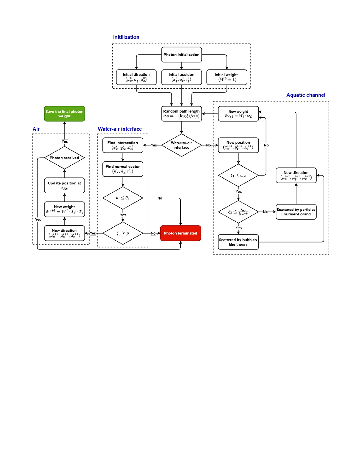
UNDER REVIEW , 2025 1 End-to-End Optical Propagation Modeling for W ater -to-Air Channels under Sea Surface and U A V Ef fects M. Nennouche, M.A. Khalighi, A.A. Do whuszko, and D. Merad Abstract —Underwater observatories ha ve recently emerged as an efﬁcient mean of marine biodiversity monitoring. In order to conduct data muling from the underwater sensors in an efﬁcient and cost-effective way , we consider the use of optical wireless communications to transmit the data from the underwater sensors to an aerial node close to the water surface, such as an unmanned aerial vehicle (U A V). More speciﬁcally , we utilize a direct water-to-air (W2A) optical communication link between the sensor node equipped with an LED emitter and the U A V equipped with an ultra-sensitive receiv er , i.e., a silicon photo-multiplier (SiPM). T o characterize this particularly complex communication channel, we introduce a ray-tracing algorithm based on the Monte Carlo method, incorporating the impact of bubbles modeled through the Mie scattering theory and a realistic sea surface repr esentation derived from the JON- SW AP spectrum. Additionally , we incorporate into this model the channel losses resulting from U A V instability under windy weather conditions. Furthermor e, we conduct a compr ehensive analysis of the wireless channel, examining the inﬂuence of key parameters such as wind speed, transmitter conﬁgurations, and receiv er characteristics. Finally , we evaluate the end-to-end performance of the system by analyzing the a verage bit-error rate at varying depths and data rates, pro viding valuable insights into the feasibility and efﬁciency of the proposed approach. Index T erms —Channel characterization, Marine biodiversity monitoring, Monte Carlo simulations, Silicon photo-multipliers, Underwater sensor networks, Underwater wireless optical com- munications, W ater -to-air transmission. I . I N T RO D U C T I O N T HERE has been a growing interest in the underwater world ov er the past decades, driv en by applications such as en vironmental monitoring, infrastructure inspection, and resource e xploration and exploitation. This interest has given rise to the concept of the internet of underwater things (IoUT) [1], which focuses on gathering data from underwater sensor nodes and transmitting it to remote locations for follo w-up processing and storage. Achieving high-speed, low-latency , and reliable communication in such challenging en vironments has recently become a focal point of intensi ve research [2]–[4]. This work was partly supported by the French P ACA (Provence, Alpes, C ˆ ote d’Azur) Regional Council and the ´ Ecole Centrale M ´ editerran ´ ee, Mar- seille, France. It was also based upon work from COST Action CA19111 (European Network on Future Generation Optical Wireless Communication T echnologies, NEWFOCUS), supported by COST (European Cooperation in Science and T echnology). M. Nennouche is with Aix-Marseille University , CNRS, Centrale Med, LIS, Marseille, France (e-mail: mohamed.nennouche@centrale-med.fr). M.A. Khalighi is with Aix-Marseille University , CNRS, Centrale Med, Fresnel Institute, Marseille, France (e-mail: ali.khalighi@fresnel.fr) A.A. Dowhuszk o is with Department of Information and Communication Engineering, Aalto Univ ersity , Espoo, Finland (e-mail: alexis.do whuszko@aalto.ﬁ) D. Merad is with Aix-Marseille University , CNRS, LIS, Marseille, France (e-mail: djamal.merad@lis-lab .fr) Corresponding author : M.A Khalighi Giv en the fundamental dif ferences in signal propagation through air and water media, dif ferent wireless technologies can be used, e.g., radio-frequency (RF) communications in air and acoustic/optical wireless communications in water . T o bridge these two propagation media, i.e., the underwater and the air channels, most of the previously reported approaches in the literature have considered the use of a relay node posi- tioned on the water surface, such as a buo y or an autonomous surface vehicle (ASV) [5]. This way , data from underwater sensors is transmitted to the surface node, either directly , or via an underwater drone or autonomous underwater vehicle (A UV) when the sensors are located at relativ ely large depths [6]. The surface node then relays the data through an RF link to an unmanned aerial vehicle (U A V) or a low-earth orbit (LEO) satellite, for instance [7]. Recently , a new approach has been considered in the lit- erature, which consists of direct communication through the sea surface, known as water -to-air (W2A) communication [8], [9]. This method represents a viable alternative to relay-based approaches in numerous relev ant application scenarios. For instance, in the context of coral reef monitoring, this approach is particularly well-suited since coral reefs are typically located in shallo w waters (at depths smaller than 50 m ) 1 , due to their dependence on microscopic algae (Zooxanthellae) with which they liv e in symbiosis not far from the coast, at typically less than 30 km distance [10], [11]. By utilizing W2A communication, data collection can be achieved without the need for expensiv e underwater drones or ASVs, or the deployment of surface buo ys, which often require anchoring that could disrupt and damage the delicate ecosystem under study . A. Underwater W ireless Optical Communications Underwater communications hav e traditionally been domi- nated by acoustic links, primarily due to the low attenuation of acoustic signals in water, enabling communication ov er lar ge ranges of up to sev eral kilometers [12], [13]. Howe ver , the limited communication bandwidth and slow propagation speed of acoustic signals result in very lo w data rates and signiﬁcant latency . In addition, several studies ha ve demonstrated the harmful effect of acoustic wav es on underwater ecosystems [14]. As a result, there has been increasing interest in under- water wireless optical communication (UWOC), which of fer substantially higher data rates and lo wer latenc y [3], [15], as well as a lower en vironmental impact [16], thus making them more suitable for various IoUT applications, particularly in 1 Some e xamples include the New Caledonian barrier reef, the Loyalty Islands lagoons, the Mayotte coral reefs, the R ´ eunion lagoons, etc. UNDER REVIEW , 2025 2 Fig. 1. Illustration of the considered W2A wireless optical link en vironmental monitoring. These advantages, ho wever , come at the cost of reduced link range, typically limited to a fe w tens of meters in clear waters [4]. This range limitation is attributed to several impairments, including absorption, scattering, point- ing errors, background noise, and oceanic turbulence [5], [17], [18]. Here, to further reduce the potential impact on the marine ecosystem, it is crucial to limit the intensity of emitted optical signals, which can be based on using light-emitting diodes (LEDs) or laser diodes (LDs). Indeed, excessi vely high transmit optical power could negati vely impact the surrounding ﬂora and fauna [9]. Then, to maintain reliable communication ov er the typical link ranges from tens to hundred meters, it is imperati ve to use highly sensitive photodetectors (PDs) at the receiv er (Rx) side. In this study , we explore the use of silicon photomultipliers (SiPMs), also known as multi- pixel photon counters (MPPCs), which are arrays of single photon avalanche diodes (SP ADs), that offer key advantages including very high internal gain, ease of implementation, and mechanical robustness [19]–[21]. B. Communication Acr oss the Sea Surface The direct W2A optical wireless communication approach introduces additional complexities to achieving reliable link establishment, primarily due to the dynamic and random nature of the sea surface. These time-dependent variations of the sea surface are inﬂuenced by numerous uncontrollable en viron- mental factors, such as surface wind speed and underwater topography . These factors affect the optical link by causing intensity losses as well as reﬂection and refraction of the optical beam as it traverses the W2A interface. Furthermore, near the surface, wave motion generates a population of bub- bles of v arying sizes. These b ubbles contribute to additional refraction and reﬂection effects and induce oceanic turb ulence, which may eventually compromise the reliability of the optical wireless link. A critical aspect in this context is the accurate modeling of the W2A wireless channel, which is essential for designing and e valuating the performance of the communication link between the underwater sensor node and the ﬂying UA V. While there is a rich literature on channel modeling for UWOC and free-space optical communication [18], [22]–[24], realistic modeling of the effect of the sea surface variations and the impact of air bubbles, surface wav es, and U A V instability on the intensity of the received signal requires particular attention. Note, realistic sea surface modeling has been extensi vely studied by the oceanography community with a variety of models proposed so far . C. Use of UA Vs in Open Ocean En vir onments In recent years, U A Vs have emerged as versatile and cost- effecti ve platforms for advancing maritime wireless com- munication systems [25]. Their rapid deployment capability and mobility make them particularly suitable for open-ocean en vironments, where traditional infrastructures are either un- av ailable or prohibitiv ely expensiv e. U A Vs can establish links with ASVs, ﬂoating relay buoys [25], [26], or directly with underwater objects, thereby supporting critical applications such as deep-sea e xploration, environmental monitoring, and disaster-response operations. Nev ertheless, the inte gration of U A Vs into maritime com- munication networks introduces signiﬁcant challenges. Their performance is highly sensitive to meteorological conditions, especially wind, which induces vibrations, link misalignment, and ﬂuctuations in the angle of signal reception [26], [27]. Although these effects have been in vestigated in the litera- ture for both RF and optical wireless systems [26]–[29], a rigorous characterization of U A V dynamics under different lev els of wind disturbances, as well as their impact on optical W2A links remains largely unexplored. T o the best of our knowledge, this study is the ﬁrst to propose a comprehensi ve modeling framework capturing UA V vibration behavior as a function of wind speed in the context of optical W2A communication. D. P aper Contributions This work focuses on the conte xt of coral reef monitoring, where environmental sensing data collected by an underwater sensor are transmitted via an W2A optical link to a ﬂying U A V. 2 This application scenario is depicted in Fig. 1. T o simplify the design of the underwater node, the transmitter (Tx) at depth d water employs an LED optical source, while the U A V, positioned at height d air abov e the sea surface, is equipped with an SiPM-based optical Rx. As a very sensitiv e photo-detector is used, data mulling from the sensor to the U A V is assumed to be performed at night to minimize the effect of background noise [30]. W e conduct a comprehensiv e analysis of the W2A channel through accurate modeling and characterization, accounting for the effects of absorption and scattering caused by under - water particles and air bubbles, as well as the inﬂuence of surface wa ve and UA V instability under varying wind speeds. T o account for the effect of surface waves, we adopt the joint 2 When a wireless sensor network is deployed, one node typically serves as the coordinator, collecting data from all sensor nodes and transmitting them to the aerial node. The W2A link under consideration will then correspond to that between the coordinator node and the U A V. UNDER REVIEW , 2025 3 north sea wav e project (JONSW AP) model [31], which is widely accepted within the oceanography research community [32]–[34]. In particular , this model incorporates a key param- eter , i.e., the distance between the area of study (with wind activity at the sea surface) and the seashore. This parameter is particularly relev ant for coral reef studies, as these natural en vironments are typically located a fe w kilometers from the coasts [10]. On the other hand, in order to account for the effect of air b ubbles, we propose to use the Hall-No varini (HN) model [35], [36], which describes the distrib ution of the b ubble population as a function of depth. Additionally , we apply the Mie theory [37] to quantify the scattering effects introduced by these air bubbles. Finally , as an important consideration, we incorporate a study of the ef fect of U A V instability induced by turbulent wind conditions, represented through the Dryden model [38], [39]. These considerations allow a comprehensiv e and realistic characterization of the W2A channel, which is critical for link design and performance ev aluation. T o characterize the W2A channel, we employ Monte Carlo simulations [23] to model photon propagation across the wire- less link, encompassing both underwater and aerial segments. Subsequently , we incorporate the channel loss induced by U A V instability , for which we deriv e a closed-form expression. T o the best of our knowledge, this study is the ﬁrst to provide a closed-form formulation of U A V tilt angle variations and the corresponding loss in the context of optical wireless communications. W e examine the impact of v arious system parameters, including the LED beam diver gence and the ﬁeld-of-view (FoV) of the Rx, and the end-to-end (E2E) link performance. This performance is ev aluated in terms of the bit-error-rate (BER), providing insights into the practical feasibility of the proposed approach. The key contributions of this w ork can be summarized as follows: • A realistic coral reef monitoring system using W2A optical communication is inv estigated; • A comprehensive framew ork for accurately modeling the W2A channel is proposed, incorporating different factors such as underwater absorption/scattering, air bubbles, and surface wa ve motion; This is in particular based on the most appropriate models, i.e., the JONSW AP model to account for the sea surface motion in near-shore application scenarios, and the HN distribution and the Mie theory to account for the effect of air b ubbles; • A closed-form expression for channel loss due to U A V deﬂection angle is deriv ed as a function of wind speed under turbulent wind conditions, modeled by the Dryden spectrum; • A detailed E2E link performance analysis is presented, in particular , ev aluating the effect on the BER performance of Rx depth for dif ferent data rates, and demonstrating the feasibility of optical W2A communication in en vironmental monitoring applications. The remainder of this paper is or ganized as follows: Sec- tion II presents a brief state-of-the-art on W2A optical channel modeling and link design, whereas, Section III describes in detail the proposed channel modeling to account for several factors such as underwater beam absorption and scattering, random sea surface, air bubbles, and UA V instability . Af- terwards, Section IV presents our new approach to modeling losses resulting from drone instability . Subsequently , Section V details the Monte Carlo algorithm that has been developed to model photon propagation, while Section VI presents the numerical results, focusing on channel modeling and perfor - mance e valuation of the wireless link. Finally , Section VII draws the main conclusions of this work. I I . S TA T E - O F - T H E - A RT O N W 2 A O P T I C A L C O M M U N I C A T I O N S In recent years, there has been growing interest in W2A wireless optical communication, focusing on both channel modeling and link performance ev aluation. Sev eral recent studies ha ve also conducted experiments to assess W2A link performance, utilizing indoor test-beds such as water tanks or pools, as well as outdoor setups in harbor environments. For instance, in [40], Sun et al. e xperimentally demonstrated a high-speed W2A link using an ultraviolet LED and different modulation schemes, and analyzed the link performance in terms of transmission rate under the conditions of both perfect beam alignment and slight misalignment (on the order of a few centimeters) in the presence of wav es of up to 15 mm in height. More recently , Lin et al. proposed in [41] a prototype based on multiple-input multiple-outputs (MIMO) technique, using 4 blue LEDs and 4 av alanche photodiodes (APDs), as well as spatial optical ﬁltering to reduce the impact of background radiations. Through a series of experiments conducted in a water tank and in a swimming pool, they demonstrated the per - formance impro vement achie ved using the MIMO technique and error correction coding. Nev ertheless, in the en vironmental monitoring application under consideration, conducting experiments that accurately reﬂect the real-world conditions of the open sea, with wav es reaching se veral meters in height, is highly challenging. There- fore, simulation-based approaches, such as those based on Monte Carlo algorithms, represent the most suitable way for channel characterization and modeling. A critical aspect of these simulations is the realistic modeling of the air-w ater interface. One established model is the Pierson–Moskowitz (PM) model [42], which, for instance, was used in [43] to study the spatial distribution of the W2A channel loss and its temporal ev olution under varying wind speeds. Using this model, system performance with multiple Txs and/or Rxs was analyzed and e xperimentally validated in [44]. Another notable approach for the air-water interface modeling is the three- dimensional ECKV 3 model [45], which was used in [46] to in vestigate the W2A channel. The authors of [46] also studied the impact of air bubbles in the underwater channel and solar background noise considering a laser-based Tx and an APD- based Rx. Both PM and ECKV models offer realistic sea-surface modeling but are primarily applicable to systems deployed in 3 Standing for the initials of the authors’ names: Elfouhaily , Chapron, Katsaros, and V andemark. UNDER REVIEW , 2025 4 the open sea, i.e., at typically sev eral hundred kilometers from the sea shore. T o the best of our knowledge, to date, no prior studies have in vestigated the optical W2A channel in near- shore en vironments, where the JONSW AP model becomes particularly relev ant for capturing the unique dynamics of such scenarios. I I I . W 2 A C H A N N E L M O D E L I N G In this section, we de velop appropriate mathematical models for the four key components that need to be considered for modelling the W2A channel, i.e., the underwater medium, the W2A interface, the effect of air bubbles near the sea surface, and the instability of the U A V due to the wind speed. Accordingly , we present the mathematical foundations underlying the calculation of the associated losses. The W2A channel loss h can be modeled as: h = h α h MC , (1) where, h α and h MC denote the orientation-induced loss re- sulting from U A V tilting under wind effects, and the channel loss accounting for the ensemble of attenuation in water , air bubbles effect, and sea surface ﬂuctuations, respectively . In Section IV, we derive the analytical expression of h α , and subsequently , in Section V, we introduce our Monte-Carlo simulator used for estimating h MC . A. Modeling Optical Propa gation in W ater Before reaching the sea surface, the emitted photons from the Tx pass through the underwater medium, introducing absorption and scattering [37]. As we consider the sensor node for coral reefs monitoring to be at a relatively small depth (typically lower than 50 m), we logically assume that the distrib ution of underwater particles is almost uniform [47]. Additionally , when working at relativ ely shallo w waters, we reasonably consider the effects of oceanic turb ulence caused by marine currents or temperature and salinity gradients to be negligible (a detailed justiﬁcation of this assumption is provided in Appendix VII-A). As will be detailed in Section V, we use Monte Carlo sim- ulations to model photon transport in the underwater channel. Photon scattering modeling will rely on the scattering phase function (SPF) e β ( θ ) , which provides the scattering angle θ s of a photon after interaction with a particle. T o obtain samples of θ s , a random variable ξ β , uniformly distrib uted between 0 and 1 , denoted here by U (0 , 1) , will be generated to solve the following equation: ξ β = 2 π Z θ s 0 e β ( θ ) sin θ dθ . (2) The most commonly used SPF is the Henyey-Greenstein (HG) function [23], [44], [48], [49] described by: e β HG ( θ s , g HG ) = 1 − g 2 HG 4 π (1 + g 2 HG − 2 g HG cos θ s ) 3 / 2 , (3) where g HG is the mean cosine angle in all directions. The interest of the HG function is mainly due to the simplicity of its formulation and the ease of ﬁnding the scattering angle θ s using the in verse transform sampling method. That is, using a random variable ξ µ , of distribution U (0 , 1) , we obtain [23], µ HG = 1 2 g HG " 1 + g 2 HG −  1 − g 2 HG 1 − g HG + 2 g HG ξ µ  2 # . (4) Then, the samples of the scattering angle θ s are obtained as θ s = arccos µ HG . (5) Howe ver , the HG function lacks precision for small ( ≲ 20 ◦ ) and large scattering angles ( ≳ 120 ◦ ), when compared to the experimental data [23], [50], [51]. Se veral alternative SPF models hav e been proposed in the literature, where one of the most commonly used is the Fournier -Forand (FF) function [52]–[54], giv en by (6), that we will consider in this paper . e β FF ( θ s , µ FF , n s ) = 1 4 π (1 − δ ) 2 δ v  v (1 − δ ) − (1 − δ v ) +  δ (1 − δ v ) − v (1 − δ )  sin − 2 ( θ s 2 )  + 1 − δ v π 16 π ( δ π − 1) δ v π (3 cos 2 θ s − 1) . (6) Here, n s and µ FF represent the refractiv e index of the particle and the in verse power of Junge distribution 4 , respectiv ely [52], and v = 3 − µ FF 2 , δ θ = 4 3( n s − 1) 2 sin 2  θ 2  . (7) Obviously , e β FF is a more complex function than e β HG . Furthermore, since the angle θ s cannot be directly expressed as a function of ( µ FF , n s ) , we have to calculate the integral in (2) numerically . Here, to reduce the computational complexity , we use an approximation of this integral as follows [52]. ξ FF = 2 π Z θ s 0 e β FF ( θ ) sin θdθ ≈ 1 (1 − δ ) δ v  (1 − δ v +1 ) − (1 − δ v ) sin 2  θ s 2  + 1 16 π 1 − δ v π ( δ π − 1) δ v π cos θ s sin 2 θ s , (8) where ξ FF is a random v ariable of distribution U (0 , 1) . The scattering angle θ s is then obtained from ξ FF through numer- ical approximation. B. Modeling the W2A Interface Mathematical modeling of sea wav e shapes remains a challenging open problem due to the complexity and interplay of numerous contrib uting factors, such as underwater currents, atmospheric pressure, proximity to shore, surface winds, etc. Among these, surface wind speed has a particularly signiﬁcant effect, as it plays a crucial role in determining sea surface elev ation. So far , the model developed by Cox and Munk in [56] has been widely used in the literature (e.g. in [48], [49]), 4 The Junge distrib ution is a special case of a po wer law describing the size distribution of underwater particles [55]. UNDER REVIEW , 2025 5 primarily due to the simplicity of its formulation. This model proposes the sea surf ace slope in the form of a probabilistic distribution whose variance is dependent on the wind speed. Unfortunately , this purely random approach does not take into account the spatial and temporal correlation that exists in prac- tice between adjacent points of the sea surface. Consequently , other models based on the frequency and angular spectrum of wa ves have been proposed [57] such as the PM [42] and the JONSW AP models [31], previously introduced in Section II. The JONSW AP model is widely accepted in oceanography for typical wind speeds (excluding extreme cases such as hurricanes) and is considered as an ev olution of the PM model. It incorporates a so-called fetch parameter F , which represents the distance ov er which the wind interacts with the water surface and can be interpreted as the distance from the seashore. In fact, this parameter adjusts wav e heights by modifying the amplitudes of the frequency spectrum. The incorporation of this parameter is particularly relev ant in the context of this work, which aims to provide an effecti ve solution for monitoring coral reef ecosystems. Based on the JONSW AP model, we represent the sea surface elev ation z ( x, y , t ) as a sum of sinusoids, as given by (9), where ( x, y ) and t denote the spatial coordinates and time, respectiv ely [58]. z ( x, y , t ) = M X i =1 N X j =1 a ij cos( ω i t − k i x cos θ j − k i y sin θ j + ϵ ij ) (9) Here, M and N represent the numbers of frequencies and directional angles considered in the wa ve spectrum, respec- tiv ely . Also, a ij , ω i , k i , and θ j stand for the amplitude of the wa ve components, wav e angular frequency , wa ve number , and directional angle, respecti vely . Finally , ϵ ij denotes the initial phase of each wa ve component, which follows the distrib ution U (0 , 2 π ) . In ocean wa ve studies, the values of ω i are calculated as a function of the wa ve number k i as [55]: ω 2 i = g k i tanh( d 0 k i ) , (10) where d 0 represents the sea depth. For d 0 → ∞ , we use the approximation tanh( d 0 k i ) → 1 , which is commonly accepted when the sea depth signiﬁcantly exceeds the wav elength of the sea wav es under study , as is the case in this work. As a result, ω 2 i ≈ g k i . (11) On the other hand, the amplitude of each component of the wa ve a ij and the JONSW AP wav e spectrum S ( ω ) are related through the following equation, a ij = p 2 S ( ω ) D ( θ ) ∆ ω ∆ θ , (12) where D ( θ ) represents the directional spreading function, which gov erns the direction of wind evolution [58], and ∆ ω and ∆ θ denote the sampling steps in the frequenc y and angular domains, respectiv ely . Sev eral models hav e been proposed for D ( θ ) in the literature [59]. In this work, we consider the widely-used model proposed by the International T owing T ank Conference (ITTC) association [58], [60], [61], which is described by: D ( θ ) = 2 π cos 2 θ , | θ | ≤ π 2 . (13) Furthermore, the wave spectrum in (12) is calculated as [31]: S ( ω ) = α g 2 ω 5 exp  − 5 4 ( ω 0 ω ) 4  γ r , (14) where, γ = 3 . 3 , α = 0 . 075 X − 0 . 22 , (15) and X = g F /U 2 10 , with F being the fetch parameter which is set in this work to 30 km, and U 10 the average wind speed at 10 m above the sea surface. Also, r = exp  − ( ω − ω 0 ) 2 2 σ 2 ω 2 0  , (16) where σ = ( 0 . 07 , ω ≤ ω 0 , 0 . 09 , ω > ω 0 , (17) and ω 0 represents the peak angular speed of the spectrum, calculated as follows. ω 0 = 22 g U 10 X − 0 . 33 (18) C. Modeling the Effect of Air Bubbles As mentioned earlier , the mov ement of the sea surface with wa ves generates a population of bubbles near the surface [35], [46] that should be taken into account in channel modeling as their impact can be signiﬁcant. As explained, in this work, we use the widely accepted HN model [35] to account for the effect of air bubbles on optical wa ve propagation [46], [48]. For the sake of simplicity , we only take into account the scattering effect of bubbles on the optical beam, as the propagation loss within the air bubble is rather negligible. In other words, the effect of air bubbles is ev aluated considering the bubble scattering coef ﬁcient by: b bub ( z ) = N b ( z ) Q sca Ψ , (19) where N b ( z ) , Q sca , and Ψ denote the density of bubbles as a function of depth z , the mean scattering efﬁcienc y (here equal to 2 . 0 , considering particles of radius larger than 1 µ m [62]), and the mean geometric cross-sectional areas of the bubble populations, respectiv ely . T o calculate N b ( z ) , we integrate the bubble size distribution n ( r, z ) over r , which denotes the radius of the bubbles. For the HN model, this latter is gi ven by: n ( r , z ) = 1 . 6 × 10 10 G ( r , z )  U 10 13  3 exp  − z L ( U 10 )  . (20) Here, L ( U 10 ) is the so-called e-folding distance in units of meter , gi ven by: L ( U 10 ) = ( 0 . 4 , U 10 ≤ 7 . 5 m / s , 0 . 4 + 0 . 115 ( U 10 − 7 . 5) , U 10 > 7 . 5 m / s . (21) UNDER REVIEW , 2025 6 Also, G ( r, z ) in (20) is the factor that gov erns the dependence of the spectrum on radius r at a giv en depth z and is gi ven by [35]: G ( r , z ) = ( [ r ref ( z ) /r ] 4 , r min ≤ r ≤ r ref ( z ) , [ r ref ( z ) /r ] κ , r ref ( z ) < r ≤ r max , (22) where r ref refers to the reference radius of the b ubble pop- ulation in the ocean, calculated using (23), and κ = 4 . 37 + ( z / 2 . 55) 2 . r ref = 54 . 4 µ m + 1 . 984 × 10 − 6 z (23) Also, r min and r max in (22) denote the minimum and maxi- mum bubble radii, set here to 10 µ m and 1 mm, respectively , which correspond to the limits considered in the HN model [36]. Lastly , N b ( z ) and Ψ in (19) are calculated as follows [63]: N b ( z ) = Z r max r min n ( r , z ) dr ≈ (1 . 6 × 10 10 ) r 4 ref 3 r 3 min  U 10 13  3 exp  − z L ( U 10 )  , (24) Ψ = Z r max r min n ( r , z ) N b ( z ) π r 2 dr = Z r max r min 3 r 3 min r 4 ref G ( r , z ) π r 2 dr ≈ 3 π r 2 min . (25) Now , to account for the scattering ef fect of air bubbles, it is important to note that their size differs signiﬁcantly from that of typical particles in water , leading to fundamentally different scattering beha viors. In this paper , we employ Mie theory as the appropriate model to calculate the scattering angle θ s of a photon following its interaction with an air bubble [48], [63]. Based on this, we ev aluate the SPF of b ubbles e β bub as follo ws [63]: e β bub ( z , θ ) = 1 b bub Z r max r min Q b ( r , θ ) π r 2 n ( r , z ) dr , (26) where Q b ( r , θ ) ( sr − 1 ) is the scattering efﬁciency per unit solid angle in the direction θ for a single bubble with radius r . D. Effect of W ind on UA V Orientation In maritime en vironments, the frequent occurrence of wind gusts and turbulent air ﬂows can induce signiﬁcant de viations in UA V orientation [64]. Such angular instabilities directly affect the optical beam alignment and, consequently , the reliability of the W2A communication link. For most UA Vs employed in such missions, “ﬂight controllers” are used to activ ely compensate for wind disturbances through roll ( ϕ r ) , pitch ( θ p ) , and yaw ( ψ y ) adjustments, as illustrated in Fig. 2. T o model wind speed ﬂuctuations, we adopt the Dryden wind turb ulence model [39], which characterizes the amplitude of turbulence in each spatial direction, represented by e U = ( ˜ u x , ˜ u y , ˜ u z ) . Denoting the av erage and instantaneous wind speeds by vectors U = ( u x , u y , u z ) and V = ( V x , V y , V z ) , we hav e V = U + e U . Fig. 2. Axes and rotation angles of a typical quadcopter UA V that can be used for data muling in the considered coral reef monitoring scenario. T o estimate the U A V deﬂection angle α UA V under wind disturbances, we adopt the approach proposed in [65] and validated in [66], leading to the following direct relationship between α UA V and V [65]: tan( α UA V ) = 1 2 m UA V g C D ρ air A UA V V 2 , (27) where ρ air = 1 . 293 kg/m 3 denotes air density , and m UA V , C D , and A UA V correspond to the mass, drag coef ﬁcient, and equiv alent ﬂat area of the U A V. Lastly , α UA V is related to θ p and ϕ r through the following equation [65]: α UA V = arccos(cos θ p cos ϕ r ) . (28) Further details on the Dryden model are provided in Appendix VII-B. I V . S TA T I S T I C A L M O D E L I N G O F U A V I N S TAB I L I T Y Here, we introduce our methodology for modeling the impact of turbulent wind on the U A V stability based on the Dryden turbulence model [39]. W e ﬁrst deri ve a closed- form expression for the probability density function (PDF) of the U A V deﬂection angle, and subsequently formulate the corresponding channel loss. A. UA V Deﬂection Angle Modeling Let N ( µ n , σ 2 n ) denote a Gaussian distribution with mean µ n and variance σ 2 n . Based on the Dryden model, we consider V x ∼ N ( u x , σ 2 x /π ) , V y ∼ N ( u y , σ 2 y /π ) , and V z ∼ N ( u z , σ 2 z /π ) , where σ 2 x , σ 2 y , and σ 2 z denote the v ariances of wind turbulence along the three axes x , y , and z (note, a de- tailed proof of this statement is provided in Appendix VII-C). T o obtain the PDF of α UA V , we deﬁne: Z j = V j − u j σ j / √ π ∼ N (0 , 1) , j ∈ { x, y , z } , (29) which leads to V 2 = X j ∈{ x,y,z } σ 2 j π ( Z j + λ j ) 2 = X j ∈{ x,y,z } σ 2 j π χ ′ 2 1 ( λ 2 j ) , (30) where λ j = u j √ π /σ j , and χ ′ 2 1 ( λ 2 j ) denotes a non-central Chi- squared distribution with non-centrality parameter λ 2 j . Note, UNDER REVIEW , 2025 7 V 2 does not follo w a standard distribution, i.e., no simple closed-form expression is av ailable to characterize its PDF. Consequently , we propose to approximate the PDF of V 2 by a Gamma distribution, using the moment matching method with the aim of ﬁtting the ﬁrst and second order moments, i.e., E [ V 2 ] and V ar[ V 2 ] , where E [ . ] and V ar[ . ] denote the e xpected value and variance, respectively . This way , the parameters α Γ and β Γ of the corresponding Gamma distribution Γ( α Γ , θ Γ ) are calculated as follows: α Γ = [ E [ V 2 ]] 2 V ar[ V 2 ] , β Γ = V ar[ V 2 ] E [ V 2 ] , (31) where E [ V 2 ] = X j ∈{ x,y,z } σ 2 j π  1 + λ 2 j  , V ar[ V 2 ] = X j ∈{ x,y,z } σ 4 j π 2  2 + 4 λ 2 j  . (32) Consequently , the approximate PDF of V 2 , denoted here by f V 2 ( v ) , is gi ven by: f V 2 ( v ) = v α Γ − 1 exp( − v /β Γ ) Γ( α Γ ) β α Γ Γ . (33) Finally , by applying the variable change of V 2 = tan( α UA V ) /K , with K = C D ρ air A UA V 2 m UA V g , the PDF of α UA V is deriv ed as follows: f α UA V ( α UA V ) = f V 2  tan α UA V K  ·     d dα tan α UA V K     =  tan α UA V K  α Γ − 1 exp  − tan α UA V K β Γ  Γ( α Γ ) β α Γ Γ · sec 2 α UA V K . (34) B. Induced Channel Loss The ef fect of changes in the Rx’ s orientation can be modeled as a reduction in its effecti ve surface area. In other words, the corresponding induced channel loss h α can be expressed as the ratio between the actual and the effecti ve PD surface areas [67]: h α = cos α UA V Y  α UA V φ Rx  , (35) where φ Rx denotes the Rx FoV, and Q ( u ) = 1 if u ≤ 1 , and zero otherwise. Based on (34) and follo wing the same change-of-variable approach as in the previous subsection, we obtain the PDF of the orientation-induced losses f h α ( h ) as: f h α ( h α ) = f α UA V (arccos( h α ))     dα UA V dh α     = f α UA V (arccos( h α )) · 1 p 1 − h 2 α , (36) where | . | denotes the absolute value. After some mathematical manipulations, the PDF of h α is obtained as follows: f h α ( h ) = 1 K Γ( α Γ ) β α Γ Γ h − ( α Γ +1) × (1 − h 2 ) α Γ − 2 2 exp " − √ 1 − h 2 h K β Γ # . (37) V . M O N T E - C A R L O S I M U L A T I O N S F O R P H O TO N P RO PAG A T I O N There hav e been numerous research works dedicated to UWOC channel modeling based on experimental measure- ments [68], [69], analytical approaches based on the radiativ e transfer equation (R TE), e.g., [70], [71], or otherwise Monte Carlo simulations. This latter approach offers the advantage of simplicity , as it estimates the channel gain or impulse response by simulating the propagation of a large number of photons [23], [52], [72]. In this study , we employ the Monte Carlo method to analyze the channel ef fects in the W2A transmission. For this purpose, an algorithm that effecti vely incorporates the inﬂuence of the underwater channel, surface waves, and air bubbles has been dev eloped. Giv en the unique characteristics of the application scenario under consideration and the complexity and cost asso- ciated with the required extensiv e experimental measurements, this is indeed an appropriate approach for e v aluating channel effects and understanding the impact of the various phenomena on the link performance. As depicted in Fig. 1, we consider an LED at the Tx side positioned at a depth d water below the sea surface, and an SiPM PD at the Rx located at a height d air abov e the sea surface. A. Photon Pr opagation in W ater For each photon, we initialize its position, direction, and weight. The initial position of the photons ( x 0 p , y 0 p , z 0 p ) corre- sponds to the position of the Tx ( x Tx , y Tx , z Tx ) . T o initialize the photon’ s direction, considering the Lambertian radiation pattern for the LED, we need to initialize the zenith angle θ ini and the azimuthal angle ϕ ini as follows: ( θ ini = arccos[(1 − ζ θ ) 1 1+ m ] , ϕ ini = 2 π ζ ϕ . (38) Here, ζ θ and ζ ϕ are independent random v ariables with distribution U (0 , 1) , whereas m represents the LED Lam- bertian order , gi ven by m = − log 2 / log cos θ 1 / 2 , with θ 1 / 2 representing the LED half-angle [73]. In Cartesian coordinates, the photon’ s initial direction vector ( µ 0 x , µ 0 y , µ 0 z ) is then giv en by: ( µ 0 x , µ 0 y , µ 0 z ) = (cos ϕ ini sin θ ini , sin ϕ ini sin θ ini , cos θ ini ) . (39) W e set the initial weight of the photon W 0 to 1 . Then, we calculate a random step ∆ s representing the distance the pho- ton travels until interaction with a water molecule, a particle in water , or a bubble (see Subsection III-C). For this, we generate a random variable ξ , with distribution U (0 , 1) , and obtain the step as ∆ s = − log ξ /c ( z ) , where c ( z ) represents the attenuation coef ﬁcient gi ven by c ( z ) = a + b + b bub ( z ) , where a denotes the absorption coef ﬁcient, and b and b bub ( z ) represent the water and bubble scattering coef ﬁcients, respecti vely (all in units of m − 1 ) [48]. At this position, we check whether the photon has reached the sea surface. If the photon is still in UNDER REVIEW , 2025 8 water , (at step i ) we then calculate its new position (at step i + 1 ) as follows: x i +1 p = x i p + ∆ s µ i x , y i +1 p = y i p + ∆ s µ i y , z i +1 p = z i p + ∆ s µ i z . (40) T o check whether or not the photon has been de viated from its initial direction due to scattering, we generate a random variable ξ 1 with distribution U (0 , 1) , and compare it with the single scattering albedo ω al = ( b + b bub ) /c ( z ) [48]. Then, if ξ 1 ≤ ω al , we deduce that the photon has been scattered. Now , to check whether the scattering ef fect has been produced by a water molecule, a particle in water , or a bubble, we generate another random variable ξ 2 with distribution U (0 , 1) , and compare it to b bub / ( b + b bub ) [48]. Then, (i) if ξ 2 ≤ b bub / ( b + b bub ) the photon is considered to be scattered by an air bubble, in which case we calculate the new zenith angle θ s using the Mie scattering theory; (ii) otherwise, the photon is considered to be scattered by a water molecule or a particle in water , in which case we calculate θ s using the FF function. Note, in both cases, scattering is symmetrical with respect to the azimuth, and therefore, the ne w azimuthal angle ϕ s is generated considering the distribution U (0 , 2 π ) . The elements of the new direction vector are then as follows. µ i +1 x = sin θ s  µ i x µ i z cos ϕ s − µ i y sin ϕ s  q 1 − ( µ i z ) 2 + µ i x cos θ s , µ i +1 y = sin θ s  µ i y µ i z cos ϕ s + µ i x sin ϕ s  q 1 − ( µ i z ) 2 + µ i y cos θ s , µ i +1 z = − sin θ s cos ϕ s q 1 − ( µ i z ) 2 + µ i z cos θ s . (41) The photon weight is then updated as W i +1 = W i ω al . This operation is repeated as long as the photon remains in water . B. Photon Pr opagation at the W ater-Air Interface As soon as the photon reaches the sea surface, we ﬁrst determine the point of intersection with the sea surface ( x i w , y i w , z i w ) , and the vector normal to this point  n = ( ˆ n x , ˆ n y , ˆ n z ) . W e then calculate the incident angle θ i formed between the photon direction vector  µ i = ( µ i x , µ i y , µ i z ) and the normal vector as follows [44], see Fig. 3: θ i = arccos   µ i .  n ||  µ i || . ||  n ||  , (42) where ( . ) and || . || denote scalar vector product and Frobenius norm, respectiv ely . As illustrated in Fig. 3, the Snell’ s law is used to obtain the refracted angle θ r after the sea surface, before checking that θ i is not greater than the critical angle θ c = arcsin( n 2 /n 1 ) ≈ 48 . 75 o , derived from Snell’ s law , with n 1 = 1 . 33 , and n 2 = 1 the refractiv e indices of water and air , respectiv ely . If θ i > θ c , the photon will be reﬂected (i.e., remain in water) and will therefore be considered as lost. T o simulate photon propagation more realistically , we also account for the ef fect Fig. 3. Illustration of Snell’ s law at photon arri val at the water-air interface. of partial reﬂection governed by Fresnel equations [49]. As a result, a fraction of photons with an incidence angle smaller than θ c will be randomly reﬂected as well. T o consider these latter , we generate a random variable ξ 3 with distribution U (0 , 1) , and compare it with the Fresnel reﬂection coefﬁcient ρ , giv en by [49]: ρ =      1 2  h sin( θ i − θ r ) sin( θ i + θ r ) i 2 + h tan( θ i − θ r ) tan( θ i + θ r ) i 2  , if θ i  = 0 ,  n 1 − n 2 n 1 + n 2  2 , otherwise , (43) where θ r is calculated according to Snell’ s la w as follo ws: θ r = arcsin  n 2 n 1 sin θ i  . (44) Then, if ξ 3 < ρ is veriﬁed, the photon will be reﬂected and will therefore be considered as lost [49]. For photons that have not been reﬂected, we obtain their new direction using the following equation [44]:  µ i +1 = cos( θ r )  n + sin   θ r  µ i −  n (  µ i . n ||  n || )      µ i −  n (  µ i . n ||  n || )       . (45) W e also calculate the new weight W i +1 of the photon, which we consider to be unpolarized, using the Fresnel transmission coefﬁcient T f = ( T s + T p ) / 2 with T s and T p the transmis- sion coefﬁcients for the S (longitudinal) and P (transverse) components, respectiv ely: T s = sin(2 θ i ) sin(2 θ r ) sin 2 ( θ i + θ r ) , T p = sin(2 θ i ) sin(2 θ r ) sin 2 ( θ i + θ r ) cos 2 ( θ i − θ r ) . (46) In addition, giv en that the sea surface is not smooth, we consider a transmission coef ﬁcient T u , which depends on the wind speed U 10 , as follows [49]: T u =      1 − 1 . 2 × 10 − 5 U 3 . 3 10 , U 10 ≤ 9 m / s , 1 − 1 . 2 × 10 − 5 U 3 . 3 10 × (0 . 255 U 10 − 0 . 99) , U 10 > 9 m / s . (47) Then, the new photon weight is obtained as W i +1 = W i T f T u . (48) UNDER REVIEW , 2025 9 Overall, from (40), (45), (47), and (48), we can calculate the intersection position, the direction, and the weight of the photons. C. Photon Pr opagation in the Air If a photon reaches the air , it is assumed to propagate in a straight line from that point onward, as interactions between the photon and air particles are considered to be negligible. Consequently , we update the position of the photon at height z Rx . Then, two conditions should be simultaneously veriﬁed to determine whether the photon falls within the Rx’ s FoV φ Rx and activ e area of radius r Rx , namely: ( x p − x Rx ) 2 + ( y p − y Rx ) 2 <  r Rx + ( z Rx − z p ) tan φ Rx 2  2 , (49) and,  x p + µ x ( z Rx − z p ) µ z − x Rx  2 +  y p + µ y ( z Rx − z p ) µ z − y Rx  2 < r 2 Rx . (50) It is important to note that (49) and (50) assume perfect beam alignment, i.e., no inclination with respect to the optical axis. In fact, the effect of beam misalignment (corresponding to the inclination angle α UA V of the UA V caused by turbu- lent winds) is already accounted for in h α , as described in Subsection IV.IV -B. D. Monte-Carlo Channel Loss Finally , the channel loss h MC is obtained by calculating the ratio of the sum of the weights of the recei ved photons to the total number of emitted photons in the simulation. Figure 4 shows the ﬂow chart summarizing the entire algorithm. V I . N U M E R I C A L R E S U LT S This section presents the numerical results concerning the W2A channel characterization and link performance ev alua- tion. First, we illustrate the effects of sea surface wav es and air bubbles on the channel gain for different Tx/Rx parameters including the consideration of link misalignment. Then, we ev aluate the E2E link performance in terms of the average BER as a function of the LED depth for dif ferent data rates. A. System/Simulation P arameters and Main Assumptions Unless otherwise speciﬁed, we use the parameters shown in T able I for the W2A link. The considered values for the absorption and scattering coefﬁcients a and b correspond to the case of clear ocean waters [37]. Indeed, tthe validity of this assumption can be veriﬁed, for example, in [74], which reports the values of absorption and scattering coefﬁcients observed in Australian reef waters. Additionally , for the photon scattering FF SPF model (see Subsection III-A) we set the refractiv e index n s and slope parameter µ FF in (6) to 1 . 1 and 3 . 5835 , respectiv ely . These correspond to a back-scattering ratio of T ABLE I D E F AU LT W 2 A L I NK PA RA M E T ER S C O NS I D E RE D I N T HE N U M ER I C A L R E SU LT S . Parameters Symbols V alues Absorption coefﬁcient a 0 . 114 m − 1 Scattering coefﬁcient b 0 . 037 m − 1 W ater refractiv e index n 1 1 . 33 Air refractiv e index n 2 1 LED wa velength λ 470 nm LED semi-angle at half-po wer θ 1 / 2 10 o Tx position ( x Tx , y Tx , z Tx ) (0 , 0 , − 10) m Rx position ( x Rx , y Rx , z Rx ) (0 , 0 , 5) m Rx FoV φ Rx 60 o Rx activ e area radius r Rx 5 cm T ABLE II A N GU L A R F R E Q UE N C Y R A N G E ( I N RA D / S ) A N D DI R E C TI O NA L A NG L E S ( I N R A D ) U S E D F O R S E A S U R FAC E S I M U LAT IO N F O R TH E T H RE E C O NS I D E RE D W I ND S P E ED S U 10 ( I N M / S ) . U 10 [ ω l , ω h ] ∆ ω M ∆ θ N 5 [1 . 2 , 4 . 0] 0.2 15 π/ 5 6 13 [0 . 9 , 3 . 0] 0.1 22 π/ 20 21 b p = 0 . 0183 m − 1 , typical of a clear ocean [50]. Also, the fetch parameter F is set to 30 km . The Tx and the Rx are assumed to be perfectly aligned, and data transfer is carried out at night in order not to be affected by background radiations, giv en the highly sensitive SiPM that we use at the Rx. Given the relati vely small activ e area of the SiPM (see T able III), a non-imaging lens is considered in front of the PD to expand the acti ve area of the Rx without compromising its FoV. Here, the considered radius for the Rx activ e area is 5 cm. T o study the sea surface ef fect, we consider two different wind speeds 5 of U 10 = 5 , and 13 m/s. The case of U 10 = 0 , representing a ﬂat sea surface with no air bubble effects will serve as the benchmark for comparison. In the considered JONSW AP model, the values of ω i are taken within the interval [ ω l , ω h ] with a step size of ∆ ω , and the values θ j are taken within the interval [ − π/ 2 , π / 2] with a step size of ∆ θ , see (9) in Subsection III-B. These parameters are listed in T able II, where the considered parameters in the four rightmost columns are taken from [58]. Finally , we consider in this study the DJI Matrice 300 R TK U A V platform [75]. This platform was selected because it is widely employed in both industrial missions and academic research, owing to its long endurance, robustness, and ov erall reliability . Furthermore, it is designed to withstand wind speeds of up to 15 m/s, making it particularly suitable for maritime and coastal operations where gusts and turbulence are common. According to the technical speciﬁcations pro- vided in [75], the U A V has a total mass of m UA V = 8 . 37 kg (including batteries) and physical dimensions of 81 × 67 × 43 cm 3 ( L × W × H ). Since the values of A UA V and C D (see equation (27)) are not publicly av ailable, we estimated them using ANSYS software, obtaining 0 . 250 m 2 and 0 . 8 , respectiv ely . 5 The JONSW AP model is valid for U 10 between 0 and 20 m/s. UNDER REVIEW , 2025 10 Fig. 4. Flow chart of Monte Carlo photon propagation algorithm for the W2A link. B. Effect of UA V Deﬂection Angle T o inv estigate the effect of U A V instability , we ﬁrst analyze the distribution of α UA V , in order to validate the accuracy of the proposed approximate analytical PDF, f α UA V ( α ) . Fig- ures 6a and 6b contrast the simulation-based histograms of α UA V obtained from (27), with f α UA V ( α ) giv en by the closed- form expression in (34), for the two cases of U 10 = 5 and 13 m/s, respectively . First, we observe that the proposed closed-form expres- sion for the PDF pro vides an accurate approximation of the simulation-based distribution of α UA V . Second, we note the inﬂuence of increasing U 10 on the U A V’ s inclination angle: as U 10 increases, larger tilt angles with a higher variance are induced. Speciﬁcally , the standard de viation of α UA V increases from σ α = 0 . 479 ◦ at U 10 = 5 m/s to σ α = 3 . 04 ◦ at U 10 = 13 m/s, indicating reduced stability and greater v ariability under stronger wind turbulence. Nev ertheless, giv en the selected U A V (a relati vely heavy platform designed to operate under strong wind conditions) the inclination angles remain bounded. This observation is further conﬁrmed in the analysis of h α , described below . Figures 6a and 6b illustrate the distributions of h α for U 10 = 5 and 13 m/s, respectively , which are directly gov erned by the previously discussed distributions of α UA V . These results demonstrate that, owing to the selected U A V platform, the losses induced by instability remain largely negligible. It is important to emphasize that this outcome is primarily due to the use of an LED at the Tx. Indeed, the wider beam proﬁle of the LED mitigates the impact of U A V instability , conﬁrming the rationale behind this choice in the proposed system design. Employing a LD, characterized by a much narrower beam and higher sensitivity to angular deviations, would require more appropriate modeling approaches [5]. In such cases, the observ ed inclination angles could result in signiﬁcant performance degradation. A detailed in vestigation of this effect, considering a LD-based Tx and quantifying the associated losses, is planned for future work. C. Assessment of the Effect of W ave Surface and Air Bubbles First, based on the JONSW AP model, we have presented the sea surface proﬁles on a 100 × 100 m 2 grid 6 for the two considered U 10 wind speeds of 5 , and 13 m/s, in Figs. 7a, and 6 As it can be seen on the ﬁgure, the range of considered x and y grids is ( − 50 , 50) m. UNDER REVIEW , 2025 11 (a) (b) Fig. 5. Simulation-based distribution of α UA V using (27) and its analytical distribution using (34) for wind speeds: (a) U 10 = 5 m/s, and (b) U 10 = 13 m/s . 7b, respectiv ely . W e can observe the random nature of wa ve motion, along with the effect of increasing wind speed on both wa ve wav elength and peak-to-peak height. For instance, this latter increases from about 50 cm for U 10 = 5 m/s to about 1 . 5 m for U 10 = 13 m/s. As concerns air bubbles effect, using the HN model, we hav e presented in Fig. 8 the ev olution of N b ( z ) as a function of depth z for the tw o considered wind speeds U 10 . Based on this, we hav e presented in Fig. 9 the ev olution of b bub as a function of z , which clearly demonstrates the signiﬁcant v ariation in b bub near the surface. This highlights the importance of accounting for the ef fect of air bubbles on photon propagation near the water surface. Also, reasonably , higher wind speeds result in a greater concentration of air bubbles near the sea surface. D. Impact of Sea Surface W ind Speed T o study the effect of wind speed on the optical link performance, Fig. 10a shows an example of the channel gain variations over a 10 s time interv al for the two wind speeds under consideration. W e have further shown the distribution (a) (b) Fig. 6. Distribution of h α using (37) for wind speeds: (a) U 10 = 5 m/s, and (b) U 10 = 13 m/s . of the channel gain for 10000 channel realizations in Fig. 10b. These results take into account the dynamics of wav e motion, the presence of b ubbles generated by wa ve breaking, as well as the UA V deﬂection angle due to turbulent wind speed (which can be considered negligible in this study as indicated in Subsection VI.VI-B). The y clearly highlight the time-varying fading effect introduced to the channel. As a matter of fact, increased wind speed has three notable effects. First, it alters the height and wavelength of surface wav es, as illustrated in Fig. 7, leading to a higher photon loss during propagation from the Tx to the Rx due to the random effects of refraction and reﬂection at the water -air interface. Second, higher wind speeds increase the bubble population near the sea surface, resulting in a more pronounced scattering effect, as depicted in Fig. 9. Finally , the effect of wind on the UA V, as described in Subsection VI.VI-B, increases the variation of the angle α UA V with increased wind intensity , thereby inducing higher losses. For instance, from Fig. 10b we can see the destructi ve effect of increasing wind speed on the a verage W2A channel gain, which is about 1 . 58 × 10 − 5 , and 1 . 32 × 10 − 5 , for U = 5 , and 13 m/s, respectively . Interestingly , more signiﬁcant channel gain variations are UNDER REVIEW , 2025 12 (a) (b) Fig. 7. Simulated sea surfaces using the JONSW AP wav e spectrum model for the wind speeds: (a) U 10 = 5 m/s , and (b) U 10 = 13 m/s . Fig. 8. Evolution of the density number of bubbles N b ( z ) with depth z based on the HN bubble population model for different wind speeds U 10 . Fig. 9. V ariations of the scattering coefﬁcient of b ubbles b bub with depth z based on the HN bubble population model for different wind speeds U 10 . observed at lo wer wind speeds. This can be explained by the shorter wa ve periods at the surface for low U 10 values, as can be seen from Fig. 7. This increased v ariability is consistent with the ﬁndings reported in [43, Fig. 6], where a greater temporal ﬂuctuation of the channel gain was observed for U 10 = 5 m/s compared to U 10 = 10 m/s. Similar results were also presented in [44, Fig. 13], highlighting enhanced variability associated with small-scale surface wav es. E. Effect of Tx P arameters T o inv estigate the ef fect of the LED beam di vergence, we hav e shown in Fig. 11 the ev olution of the average channel gain as a function of the LED semi-angle at half-power , θ 1 / 2 . Note that, in practice, θ 1 / 2 can be adjusted using appropriate optics [76]. As expected, these results highlight the signiﬁcant impact of the LED beam diver gence on the av erage channel gain. For instance, for U 10 = 5 m/s, increasing θ 1 / 2 from 5 ◦ to 60 ◦ leads to a decrease in average channel gain from 6 . 8 × 10 − 5 to 2 . 6 × 10 − 6 , corresponding to a loss of more than 14 dB. A similar trend is observed for U 10 = 13 m/s. T o better understand these results, we hav e sho wn in Fig. 12 the spatial distribution of the channel gain at the Rx plane (i.e., at z = z Rx ). More precisely , Figs. 12a, 12b, and 12c show the distributions for U 10 = 5 m/s and θ 1 / 2 = 10 ◦ , 20 ◦ , and 30 ◦ , respectiv ely . Similarly , Figs. 12d, 12e, and 12f show the distributions for U 10 = 13 m/s. The green circle in the ﬁgures represents the equivalent activ e area of the Rx according to the assumptions in T able I. Based on the results illustrated in these ﬁgures, it can be observed that a higher beam div ergence increases photon scattering outside the Rx’ s activ e area. This, in turn, leads to greater beam refraction at the water -air interface, resulting in a higher channel loss. Note, although using a more directional beam is more adv antageous, it also increases the link sensitivity to beam misalignment (see Subsection VI.VI-G). T o study the impact of the Tx depth, we hav e shown in Fig. 13 the average channel gain as a function of d water varying from 10 to 40 m. A larger d water leads to increased photon UNDER REVIEW , 2025 13 (a) (b) Fig. 10. W2A channel gain for dif ferent wind speeds U 10 ; (a) e volution ov er a time interval of 10 s; (b) distrib ution over 10 4 channel realizations. Fig. 11. A verage channel gain as a function of the LED beam div ergence θ 1 / 2 for different wind speeds U . absorption and scattering during propagation in water , and furthermore, results in a larger beam size at the water-air interface, increasing the proportion of photons not captured on the Rx’ s equiv alent acti ve area. T o support these results, Fig. 14 shows the spatial distri- bution of the channel gain at z = z Rx for d water = 15 , 30 , and 40 m, and wind speeds U 10 = 5 , 13 m / s, while θ 1 / 2 is set to its default value of 10 ◦ . Compared to the results of Fig. 12 presented earlier, the speciﬁcity of these results is that they show an extinction phenomenon due to the absorption and scattering effect of the underwater channel with increased d water . F . Effect of Rx P arameters First, let’ s study the ef fect of the Rx height relativ e to the sea surface, denoted by d air in Fig.1. W e ha ve shown in Fig. 15 the average channel gain as a function of d air , varying between 2 and 10 m. As expected, increasing d air induces more channel loss. As pre viously established, the effects of scattering and absorption in air are ne glected in this study . Thus, the observed losses result from the cumulativ e ef fect of photon refraction at the surface, the effect of U A V instability , combined with the increasing propagation distance in air, which drastically reduces the probability of photon reception on the PD’ s active area. The signiﬁcantly higher average channel gain for the case of ﬂat sea surface (i.e., U 10 = 0 ) further conﬁrms this observation. W e have further shown in Fig. 16 the av erage channel gain as a function of the radius of the Rx equi valent activ e area. As expected, enlarging the Rx activ e area directly contributes to collecting a lar ger number of photons, and hence, to a larger channel gain. Note, in practice, the Rx active area can be dynamically adjusted alongside the Rx height using a mechanical iris mounted abov e the PD, as proposed for example in [77]. G. Effect of Beam Misalignment In practice, the communication link is affected by Tx-Rx misalignment due mainly to the limited positioning accuracy of the underwater node or the U A V. In this paper , this effect is modeled by an offset horizontal displacement δ m between the Tx and the Rx as illustrated in Fig. 17. The ef fect of this spatial offset on the average channel gain is shown in Fig. 18. W e notice a certain robustness to Tx- Rx displacements thanks to the relati vely large LED beam div ergence angle ( θ 1 / 2 = 10 ◦ ). For instance, for δ m = 0 . 5 m, the corresponding loss with respect to δ m = 0 is about 1 . 35 dB and 2 . 05 dB for U 10 = 5 and 13 m/s, respecti vely , which is consistent with the results of Figs. 12a and 12d. H. E2E Link P erformance Study Finally , this section presents the numerical results to ev al- uate the E2E link performance in terms of the av erage BER UNDER REVIEW , 2025 14 (a) (b) (c) (d) (e) (f) Fig. 12. Spatial distribution of the av erage channel gains with different LED beam div ergence angles θ 1 / 2 and wind speeds U 10 ; (a) U 10 = 5 m / s , θ 1 / 2 = 10 ◦ ; (b) U 10 = 5 m / s , θ 1 / 2 = 20 ◦ ; (c) U 10 = 5 m / s , θ 1 / 2 = 30 ◦ , (d) U 10 = 13 m / s , θ 1 / 2 = 10 ◦ , (e) U 10 = 13 m / s , θ 1 / 2 = 20 ◦ ; (f) U 10 = 13 m / s , θ 1 / 2 = 30 ◦ . The green circle in the center of all subplots represents the PD active area. Fig. 13. A verage channel gain as a function of the Tx depth d water , θ 1 / 2 = 10 ◦ and different wind speeds U 10 . for a giv en data rate R b measured in megabits per second (Mbps). The considered SiPM is the ONSE-30020 SiPM [78] component with parameters summarized in T able III (see [19] for additional description of the SiPM parameters). The considered trans-impedance ampliﬁer (TIA) load resistance is 1 k Ω . As for the Tx, we use the NICHIA NSPB510AS LED [79] with central wav elength λ = 470 nm and set the transmit power to P Tx = 100 mW; this wa velength corresponds to the maximum sensitivity of the selected SiPM. W e consider T ABLE III O N SE M I M IC R O F J - 3 00 2 0 S I P M PA RA M E T ER S [ 7 8] Parameter Symbol V alue Gain G 10 6 Number of SP ADs N SP AD 14410 Activ e area A SiPM 9 . 43 mm 2 Fill factor F F 62 % Photon detection ef ﬁciency Υ PDE 30 % Dark count rate f DCR 471 kHz Cross-talk probability P CT 2 . 5 % After-pulsing probability P AP 0 . 75 % the simple uncoded non-return to zero (NRZ) on-of f keying (OOK) modulation with extinction ratio ξ OOK = 0 . 1 . NRZ- OOK has the advantage of implementation simplicity assum- ing the need to relativ ely low to moderate data rates. Signal demodulation is performed based on optimal threshold calcu- lation, see [67] for details. Additionally , we take into account the modulation bandwidth limitation of the SiPM and the LED, which are experimentally e valuated as f c,LED = 10 MHz and f c,SiPM = 2 MHz, and model their frequency responses as ﬁrst-order low-pass ﬁlters, see [19], [20]. Figure 19 shows BER plots as a function of the Tx depth d water for the wind speeds of U 10 = 5 and 13 m/s, and different data rates R b , assuming d air = 5 m. As benchmark, we hav e also shown the BER plots for U 10 = 0 . First, we notice the performance degradation with increase in R b , which is due to the limited bandwidth of the SiPM and the LED, resulting in reduced link range [19]. For instance, for a target BER of 10 − 3 and U 10 = 0 m/s, the maximum Tx depth d water for R b = 5 and 10 Mbps is about 43 and 36 m, UNDER REVIEW , 2025 15 (a) (b) (c) (d) (e) (f) Fig. 14. Spatial distribution of the av erage channel gain at the Rx plane for different wind speeds and Tx depths: (a) U 10 = 5 m / s , d water = 15 m ; (b) U 10 = 5 m / s , d water = 30 m ; (c) U 10 = 5 m / s , d water = 40 m ; (d) U 10 = 13 m / s , d water = 15 m ; (e) U 10 = 13 m / s , d water = 30 m ; (f) U 10 = 13 m / s , d water = 40 m . θ 1 / 2 = 10 ◦ , the green circle in the center of all subplots represents the equiv alent Rx active area. Fig. 15. A verage channel gain as a function of the Rx height d air abov e the sea surface for different wind speeds U 10 . respectiv ely . Note that, frequency-domain equalization can be employed to improve the ef fectiv e link range, as considered in [20]. Second, we notice the substantial performance degrada- tion with the surface wind ef fect. F or instance, for U 10 = 5 m/s and the same target BER of 10 − 3 , the link range is reduced by 4 and 5 m for R b = 5 and 10 Mbps, respectively , with respect to the ﬂat surface case (i.e., U 10 = 0 ). W e can also observe the performance degradation with increase in U 10 : for a tar get BER of 10 − 3 , the link range is reduced by ≈ 2 . 5 m Fig. 16. A verage channel gain as a function of the Rx radius for different wind speeds U 10 . by increasing U 10 from 5 to 13 m/s. Lastly , considering a typical data rate of R b = 1 Mbps in the IoUT context for transmitting underwater sensor data, and giv en the forward error correction (FEC) limit of 2 × 10 − 3 for the BER, it is quite feasible to establish UWOC links with Tx depths up to ∼ 47 m with surface wav e speeds reaching up to 13 m/s. This range of depth is in fact sufﬁcient for the intended application of coral reef monitoring. It is worth noting that the obtained performance is mainly due to the use UNDER REVIEW , 2025 16 Fig. 17. Illustration of the Tx-Rx horizontal displacement error (spatial offset) δ m . Fig. 18. A verage channel gain as a function of the Tx-Rx displacement δ m for different wind speeds U 10 . Fig. 19. A verage BER as a function of Tx depth for bit rates R b = 1 , 5 , 10 Mbps and wind speeds U 10 = 0 , 5 , 13 m / s. of a highly sensitive SiPM as the PD, and to the fact that the transmission is assumed to take place at night, i.e., in the absence of background solar noise [17], [30]. T o further validate the feasibility of reliable link deploy- ment, we ev aluate the noise equiv alent power (NEP) of the SiPM using the following expression [80]: NEP( λ ) = E ph F e p f c,SiPM Υ PDE 1 + s 1 + 2 f DCR f c,SiPM ! , (51) where E ph = h p c p /λ denotes the photon ener gy correspond- ing to the wav elength λ , with h p and c p being Planck’ s constant and the light celerity , respectively . Also, Υ PDE and f DCR represent the SiPM’ s photon detection efﬁcienc y and dark count rate, respectively , and F e is its excess noise factor , giv en by [80]: F e = 1 1 + ln(1 − P CT − P AP ) . (52) Here, P CT and P AP denote the probabilities of optical cross- talk and after-pulsing, respecti vely . The SiPM’ s NEP, in fact, represents the incident optical power required to yield a unit signal-to-noise ratio (SNR) at the detector output. Accordingly , the equiv alent optical noise power can be expressed as P n = NEP( λ ) √ B , where B denotes the ef fective noise bandwidth [81]. For the selected SiPM with parameters listed in T able III, we obtain a NEP of 3 . 42 × 10 − 15 W / √ Hz at the considered wa ve- length λ = 470 nm. Assuming the approximate equiv alent noise bandwidth as B ≈ R b / 2 for the considered NRZ-OOK signaling, the corresponding equiv alent noise power equals P n = 2 . 42 × 10 − 12 , 5 . 41 × 10 − 12 , and 7 . 65 × 10 − 12 W for R b = 1 , 5 , and 10 Mbps, respectively [81]. This ensures a sufﬁciently high SNR for reliable communication over the considered ranges. For instance, for U 10 = 13 m/s and R b = 1 Mbps, the system achieves an av erage electrical SNR of approximately 15 . 63 dB for d water = 47 m at the SiPM output, resulting in a BER below the FEC limit (as mentioned in the last paragraph of the previous page). Neglecting the ef fects of surface wav es, air bubbles, and U A V instability , using [67, Eq. 3], the corresponding SNR is about 28 . 64 dB. This means we need a link margin of about 13 dB to compensate the channel random effects in this example. V I I . C O N C L U S I O N S In this work, we presented a comprehensi ve channel char- acterization and modeling for W2A optical wireless commu- nications for the purpose of marine ecosystem monitoring. The proposed approach uses a Monte Carlo-based ray-tracing algorithm that incorporates key parameters of the underwater channel on photon propagation, and accounts for the ef fects of sea surface through the JONSW AP spectrum model, as well as air b ubbles near the sea surface through Mie theory and the HN model. In addition, we proposed a new model to characterize the impact of UA V instability under turbulent wind conditions on the W2A link. This way , critical en vironmental factors such as wind speed and distance to the seashore, which are particularly relev ant for coral reef studies, are taken into account. UNDER REVIEW , 2025 17 Fig. 20. Geographical location of the three A ODN temperature and salinity measurement stations studied in this work based on data from [82]. Based on the thoughtful choice of JONSW AP and HN models and considering realistic parameters for a typical IoUT system for coral reef monitoring, we in vestigated the impact of the instability of the U A V, the wind speed and air bubbles, Tx and Rx parameters, including as well the impact of link misalignment. Finally , the E2E link performance analysis demonstrated the viability of the proposed system for coral reef monitoring, achieving a data rate of R b = 1 Mbps at depths of up to 47 meters and with wind speeds of up to 13 m/s. In summary , this work provides essential insights and guidelines for designing IoUT systems with W2A optical links tailored to marine biodiv ersity monitoring. The proposed photon propagation algorithm serves as a valuable tool for further exploration of the W2A communication channel, in view of dev eloping robust systems capable of mitigating the effects of bubbles and sea surface dynamics. A P P E N D I X A. T emperatur e and Salinity Pr oﬁles in Coral Reef W aters Oceanic turbulence has been extensi vely inv estigated in the ﬁeld of UWOC, primarily in the context of v ertical links [5], [18]. This is because the phenomenon is typically caused by temperature and salinity gradients across different ocean layers, which can lead to deviations of the optical beam [55]. In fact, these gradients are not uniform across all oceans, as illustrated in [18, Fig. 1]. As brieﬂy discussed in Section III, in this work, we assume that the temperature and salinity gradients are negligible, which allows us to neglect the effects of oceanic turbulence in our W2A channel modeling. T o support this assumption, we present in this Appendix the temperature and salinity gradients observed in reef waters near the Great Barrier Reef of Ne w Caledonia. Our analysis relies on measurement data provided by the australian open data network (A ODN) [82]. As (a) (b) Fig. 21. Oceanic proﬁles of (a) temperature (b) salinity in three localizations near the New Caledonia Barrier reef indicated in Fig. 20. psu denotes practical salinity unit. Results are based on the data provided in [82]. shown in Fig. 20, we consider three measurement sta- tions located near the reefs of Ne w Caledonia, at coor- dinates (165 . 91 ◦ E , 21 . 17 ◦ S ) , (167 . 33 ◦ E , 22 . 11 ◦ S ) , and (165 . 45 ◦ E , 20 . 51 ◦ S ) , respectiv ely . W e have sho wn in Figs. 21a and 21b the vertical proﬁles of temperature and salinity , respectiv ely , as functions of ocean depth. It can be clearly observed that within the ﬁrst 50 meters of depth (the region of interest in this study), both temperature and salinity gradients are extremely weak. These results, corroborated by MacKellar et al. [83], indicate that oceanic turbulence ef fects can be considered negligible in the context of our analysis. B. T urbulent W ind Modeling According to Dryden Model W e consider in this work turbulent winds (i.e., with time- varying wind speed), which are commonly encountered in analyses of airﬂo w over the ocean. T o model the effect of these phenomena, here we employ the Dryden model [39], which is UNDER REVIEW , 2025 18 one of the most widely adopted approaches in the literature [38], [64]. This model is deriv ed from extensi ve measurements and experimental data, providing an empirical characterization of the power spectral density (PSD) of wind turbulence. Follo wing the methodology described in [38], the wind is modeled as the combination of a av erage wind compo- nent U = ( u x , u y , u z ) ⊤ and a turb ulent component e U = ( ˜ u x , ˜ u y , ˜ u z ) ⊤ . The Dryden model generates the turbulence velocities by ﬁltering three independent, unit variance, band- limited white Gaussian noise processes, one for each spatial direction, through transfer functions deﬁned as follows [38]: H x ( s ) = σ x s 2 L x π | U | 1  1 + L x | U | s  , H y ( s ) = σ y s L y π | U |  1 + √ 3 L y | U | s   1 + L y | U | s  2 , H z ( s ) = σ z s L z π | U |  1 + √ 3 L z | U | s   1 + L z | U | s  2 , (53) where σ x , σ y , and σ z denote the wind turbulence standard deviations, and L u , L v , and L w represent the turb ulence length scales in directions x , y , and z , respectiv ely . In this study , we follow the military standard MIL-F-8785C [84], which provides the expressions for turbulence length scales as follows: L z = d air , L x = L y = d air (0 . 177 + 0 . 000823 d air ) 1 . 2 . (54) At low altitudes (below < 1000 feet), the standard deviations take the following values [84]: σ z = 0 . 1 W 20 , σ x σ z = σ y σ z = 1 (0 . 177 + 0 . 000823 d air ) 0 . 4 , (55) where W 20 denotes the wind speed at 20 feet ( ≈ 6 m) in knots. It is typically set to 15 knots for lo w turb ulence, 30 knots for moderate turbulence, and 45 knots for high turbulence conditions. Figures 22a and 22b illustrate an example of variations of the simulated wind for u x = u y = 5 m/s along the x and y axes, respectively , under moderate turb ulence conditions. C. Distributions of T urbulent W ind Components In this appendix, we deriv e the statistical distributions of the wind velocity components, i.e., V = ( V x , V y , V z ) , using the Dryden model. T o this end, we recall the linear ﬁlters H x , H y , and H z introduced in (53). The inputs to these ﬁlters are zero- mean Gaussian white noise processes with unit v ariance, i.e., N (0 , 1) . Consequently , the outputs of the ﬁlters can be also be modeled as Gaussian random processes where, for instance, the variance corresponding to H x output giv en by: σ 2 out , x = Z + ∞ −∞ | h x ( t ) | 2 dt, (56) (a) (b) Fig. 22. V ariations of wind speed for average wind speed of u x = u y = 5 m/s (under moderate turbulence conditions) along the (a) x -axis and (b) y -axis. where h x ( t ) denotes the ﬁlter impulse response. For the variance of V x , we recall the transfer function of H x as a function of the Laplace operator s : H x ( s ) = σ x r 2 L x π U 1 1 + L x U s = K 1 + τ s , (57) where K = σ x q 2 L x π U and τ = L x /U , with U denoting the av erage wind speed and L x the turbulence length scale of H x , respecti vely . The corresponding impulse response h x ( t ) is obtained using the in verse Laplace transform: h x ( t ) = K · 1 τ e − t/τ u H ( t ) , (58) where u H ( t ) is the Heaviside unit step function. Then, the output variance is obtained by ev aluating the energy of the ﬁlter: σ 2 V x = E h x = K 2 τ 2 Z ∞ 0 e − 2 t/τ dt = K 2 2 τ = σ 2 x π . (59) A similar procedure applies to V y and V z , since H y and H z exhibit similar structures. For the sake of clarity , we provide UNDER REVIEW , 2025 19 details on the deriv ation for H y in the following: H y ( s ) = K 1 + √ 3 τ s (1 + τ s ) 2 , (60) with K = σ y p (2 L y ) / ( π U ) and τ = L y /U . By applying the in verse Laplace transform, we obtain: h y ( t ) = K √ 3 τ + 1 − √ 3 τ 2 t ! e − t/τ u H ( t ) . (61) Exploiting the following general formula, Z ∞ 0 t n e − 2 t/τ dt = n ! (2 /τ ) n +1 , (62) the total energy of the ﬁlter simpliﬁes to: E h y = Z ∞ 0 h y ( t ) 2 dt = K 2 Z ∞ 0 √ 3 τ + 1 − √ 3 τ 2 t ! 2 e − 2 t/τ dt = K 2 τ = σ 2 y π . (63) By analogy , the same result holds for V z . Thus, we establish that: σ 2 V j = σ 2 j π , j ∈ { x, y , z } . (64) Finally , by combining the turbulent components with the constant mean wind U , the resulting velocity components follow a Gaussian distrib ution as follows: V j ∼ N ( u j , σ 2 j /π ) , j ∈ { x, y , z } . (65) D I S C L O S U R E S The authors declare no conﬂicts of interest. A C K N O W L E D G M E N T The authors would like to thank Mr . Yves Chardard from SubSeaT ech Co., Marseille, France, and Mr . Djamel Eddine T ahraoui from Segula T echnologies Co., for their v aluable guidance and insightful advice regarding the modeling aspects of the U A V. They would also like to acknowledge the support receiv ed from the French South-Region Council and the Ecole Centrale Med, Marseille, France. R E F E R E N C E S [1] M. Jahanbakht, W . Xiang, L. Hanzo, and M. R. Azghadi, “Internet of underwater things and big marine data analytics - a comprehensiv e survey , ” IEEE Commun. Surve ys T uts. , v ol. 23, no. 2, pp. 904–956, Jan. 2021. [2] M. Khalighi, C. Gabriel, T . Hamza, S. Bourennane, P . L ´ eon, and V . Rigaud, “Underwater wireless optical communication; recent ad- vances and remaining challenges, ” in 16th International Conference on T ransparent Optical Networks (ICTON) , July 2014, pp. 1–4. [3] H. Kaushal and G. Kaddoum, “Underwater optical wireless communi- cation, ” IEEE Access , vol. 4, pp. 1518–1547, Apr . 2016. [4] X. Sun, C. H. Kang, M. Kong, O. Alkhazragi, Y . Guo, M. Ouhssain, Y . W eng, B. H. Jones, T . K. Ng, and B. S. Ooi, “ A review on practical considerations and solutions in underwater wireless optical communication, ” J. Lightw . T echnol. , vol. 38, no. 2, pp. 421–431, Jan. 2020. [5] I. C. Ijeh, M. A. Khalighi, M. Elamassie, S. Hranilovic, and M. Uysal, “Outage probability analysis of a vertical underwater wireless optical link subject to oceanic turbulence and pointing errors, ” IEEE/OSA J . Opt. Commun. Netw . , vol. 14, no. 6, pp. 439–453, May 2022. [6] K. A. Mahmoodi and M. Uysal, “Energy aware trajectory optimization of solar po wered A UVs for optical underwater sensor networks, ” IEEE T rans. Commun. , vol. 70, no. 12, pp. 8258–8269, Oct. 2022. [7] A. Gupta, N. Sharma, P . Garg, D. N. K. Jayakody , C. Y . Aleksandrovich, and J. Li, “ Asymmetric satellite-underwater visible light communication system for oceanic monitoring, ” IEEE Access , vol. 7, pp. 133 342– 133 350, Aug. 2019. [8] H. Luo, J. W ang, F . Bu, R. Ruby , K. W u, and Z. Guo, “Recent progress of air/water cross-boundary communications for underwater sensor networks: A re view , ” IEEE Sensors J. , vol. 22, no. 9, pp. 8360– 8382, Mar . 2022. [9] L.-K. Chen, Y . Shao, and Y . Di, “Underwater and water -air optical wireless communication, ” J. Lightw . T echnol. , v ol. 40, no. 5, pp. 1440– 1452, Nov . 2022. [10] P . Bouchet, P . Lozouet, P . Maestrati, and V . Heros, “ Assessing the mag- nitude of species richness in tropical marine en vironments: exceptionally high numbers of molluscs at a new caledonia site, ” Biol. J. Linn. Soc. , vol. 75, no. 4, pp. 421–436, Apr . 2002. [11] K. M. Morgan, C. T . Perry , S. G. Smithers, J. A. Johnson, and J. J. Daniell, “Evidence of e xtensiv e reef dev elopment and high coral co ver in nearshore en vironments: implications for understanding coral adaptation in turbid settings, ” Sci. Rep. , v ol. 6, no. 1, p. 29616, July 2016. [12] M. F . Ali, D. N. K. Jayakody , Y . A. Chursin, S. Affes, and S. Dmitry , “Recent advances and future directions on underwater wireless commu- nications, ” Ar ch. Comput. Methods Eng. , vol. 27, pp. 1379–1412, Aug. 2020. [13] W . Jiang and R. Diamant, “Long-range underwater acoustic channel estimation, ” IEEE T rans. W ir eless Commun. , vol. 22, no. 9, pp. 6267– 6282, Feb . 2023. [14] A. N. Popper and A. D. Hawkins, “ An ov erview of ﬁsh bioacoustics and the impacts of anthropogenic sounds on ﬁshes, ” J. Fish Biol. , vol. 94, no. 5, pp. 692–713, Mar. 2019. [15] M. A. Khalighi, C. J. Gabriel, L. M. Pessoa, and B. Silva, V isible Light Communications: Theory and Applications . CRC-Press, 2017, ch. Underwater V isible Light Communications, Channel Modeling and System Design, pp. 337–372. [16] A. Bassi, O. P . Love, S. J. Cooke, T . R. W arriner, C. M. Harris, and C. L. Madliger , “Effects of artiﬁcial light at night on ﬁshes: A synthesis with future research priorities, ” F ish F ish. , vol. 23, no. 3, pp. 631–647, Dec. 2021. [17] T . Hamza, M. A. Khalighi, S. Bourennane, P . L ´ eon, and J. Opderbecke, “In vestigation of solar noise impact on the performance of underwater wireless optical communication links, ” Opt. Expr ess , v ol. 24, no. 22, pp. 25 832–25 845, Oct. 2016. [18] M. Elamassie and M. Uysal, “V ertical underwater visible light com- munication links: Channel modeling and performance analysis, ” IEEE T rans. Commun. , vol. 19, no. 10, pp. 6948–6959, July 2020. [19] M. A. Khalighi, T . Hamza, S. Bourennane, P . L ´ eon, and J. Opderbecke, “Underwater wireless optical communications using silicon photo- multipliers, ” IEEE Photonics J. , vol. 9, no. 4, July 2017. [20] M. A. Khalighi, H. Akhouayri, and S. Hranilo vic, “Silicon- photomultiplier-based underw ater wireless optical communication using pulse-amplitude modulation, ” IEEE J. Ocean. Eng. , vol. 45, no. 4, pp. 1611–1621, July 2019. [21] SensL, Intr oduction to SiPM, T echnical Note . ON Semiconductor ® - SensL, 2011 (Rev . 6.0, Feb. 2017), a vailable at https://www .sensl.com/ downloads/ds/TN \ %20- \ %20Intro \ %20to \ %20SPM \ %20T ech.pdf. [22] B. Cochenour, L. Mullen, and J. Muth, “T emporal response of the underwater optical channel for high-bandwidth wireless laser communi- cations, ” IEEE J. Ocean. Eng. , vol. 38, no. 4, pp. 730–742, Oct. 2013. [23] C. Gabriel, M.-A. Khalighi, S. Bourennane, P . L ´ eon, and V . Rigaud, “Monte-carlo-based channel characterization for underwater optical communication systems, ” IEEE/OSA J. Opt. Commun. Netw . , v ol. 5, no. 1, pp. 1–12, Dec. 2012. [24] M. A. Khalighi and M. Uysal, “Survey on Free Space Optical Communi- cation: A Communication Theory Perspecti ve, ” IEEE Commun. Surveys T uts. , vol. 16, no. 4, pp. 2231–2258, Nov . 2014. [25] N. Nomikos, P . K. Gkonis, P . S. Bithas, and P . T rakadas, “ A surve y on UA V-aided maritime communications: Deployment considerations, applications, and future challenges, ” IEEE Open J . Commun. Soc. , vol. 4, pp. 56–78, Nov . 2022. [26] S. N. Pottoo, P . G. Ellingsen, and T . D. Ho, “Evaluations of U A V-enabled FSO communications in the arctic, ” in 2022 IEEE/SICE Int. Symp. on Sys. Inte gration (SII) . IEEE, Jan. 2022, pp. 297–302. UNDER REVIEW , 2025 20 [27] Z. Liu, E. Zhou, J. Cui, Z. Dong, and P . Fan, “ A double-beam soft handover scheme and its performance analysis for mmW ave UA V communications in windy scenarios, ” IEEE T rans. V eh. T echnol. , vol. 72, no. 1, pp. 893–906, Sept. 2022. [28] P . Agheli, H. Beyran vand, and M. J. Emadi, “U A V-assisted underwater sensor networks using RF and optical wireless links, ” J. Lightw . T echnol. , vol. 39, no. 22, pp. 7070–7082, Sept. 2021. [29] S. Nie et al. , “mmW ave on a farm: Channel modeling for wireless agricultural networks at broadband millimeter-w ave frequency , ” in An- nual IEEE Int. Conf. on Sensing, Commun., and Networking (SECON) . IEEE, Sept. 2022, pp. 388–396. [30] T . Hamza and M. A. Khalighi, “On limitations of using silicon photo- multipliers for underwater wireless optical communications, ” in 2019 2nd W est Asian Colloq. on Opt. W ir eless Commun. (W ACO WC) . IEEE, Apr . 2019, pp. 74–79. [31] K. Hasselmann, T . P . Barnett, E. Bouws, H. Carlson, D. E. Cartwright, K. Enke, J. Ewing, A. Gienapp, D. Hasselmann, P . Kruseman et al. , “Measurements of wind-wave growth and swell decay during the joint north sea wav e project (jonswap). ” Er gaenzungsheft zur Deutschen Hydr ographisc hen Zeitschrift, Reihe A , 1973. [32] M. Ryabkov a, V . Karaev , J. Guo, and Y . T itchenko, “ A revie w of wa ve spectrum models as applied to the problem of radar probing of the sea surface, ” J. Geophys. Res. Oceans , v ol. 124, no. 10, pp. 7104–7134, Oct. 2019. [33] U.-J. Lee, W .-M. Jeong, and H.-Y . Cho, “Estimation and analysis of JONSW AP spectrum parameter using observed data around Korean coast, ” J. Mar . Sci. Eng. , vol. 10, no. 5, p. 578, Apr . 2022. [34] J. G. Rueda-Bayona, A. Guzm ´ an, and J. J. Cabello Eras, “Selection of JONSW AP spectra parameters during water-depth and sea-state transitions, ” J . W aterw . P ort Coast. Ocean Eng. , vol. 146, no. 6, p. 04020038, July 2020. [35] R. S. K eiffer , J. C. Novarini, and G. V . Norton, “The impact of the background bubble layer on reverberation-deri ved scattering strengths in the low to moderate frequency range, ” J. Acoust. Soc. Am. , vol. 97, no. 1, pp. 227–234, Jan. 1995. [36] M. A. Ainslie, “Effect of wind-generated b ubbles on ﬁxed range acoustic attenuation in shallow water at 1–4khz, ” J. Acoust. Soc. Am. , vol. 118, no. 6, pp. 3513–3523, Dec. 2005. [37] C. D. Mobley , Light and water: radiative transfer in natural waters . CRC-Press, 1994. [38] A. Kachroo et al. , “Emulating U A V motion by utilizing robotic arm for mmW ave wireless channel characterization, ” IEEE Tr ans. Antennas Pr opag. , vol. 69, no. 10, pp. 6691–6701, Apr . 2021. [39] M. Standard, “Flying qualities of piloted aircraft, ” US Dept. of Defense MIL-STD-1797A , 1990. [40] X. Sun, M. K ong, C. Shen, C. H. Kang, T . K. Ng, and B. S. Ooi, “On the realization of across wavy water-air-interf ace diffuse-line-of-sight communication based on an ultraviolet emitter , ” Opt. Express , vol. 27, no. 14, pp. 19 635–19 649, June 2019. [41] T . Lin, T . W ei, Q. Hu, C. Fu, N. Huang, X. Liu, L. T ang, L. Su, J. Luo, and C. Gong, “Real-time water-to-air communication system under dynamic water surface and strong background radiation, ” IEEE Photonics J. , May 2024. [42] W . J. Pierson Jr and L. Moskowitz, “ A proposed spectral form for fully dev eloped wind seas based on the similarity theory of SA Kitaigorod- skii, ” J. Geophys. Res. , vol. 69, no. 24, pp. 5181–5190, Dec. 1964. [43] T . Lin, C. Gong, J. Luo, and Z. Xu, “Dynamic optical wireless communication channel characterization through air-water interface, ” in IEEE/CIC Int. Conf. on Commun. in China (ICCC W orkshops) . IEEE, Sept. 2020, pp. 173–178. [44] T . Lin, C. Fu, T . W ei, N. Huang, X. Liu, L. T ang, L. Su, J. Luo, and C. Gong, “W aving effect characterization for water-to-air optical wireless communication, ” J. Lightw . T echnol. , vol. 41, no. 1, pp. 120– 136, Oct. 2022. [45] T . Elfouhaily , B. Chapron, K. Katsaros, and D. V andemark, “ A uniﬁed directional spectrum for long and short wind-driven wav es, ” J. Geophys. Res. Oceans , vol. 102, no. C7, pp. 15 781–15 796, July 1997. [46] B. R. Angara, P . Shanmugam, H. Ramachandran, and C. G. Sandhani, “Performance assessment of underwater-to-air optical wireless commu- nication system with the ef fect of solar noise and sea surface conditions, ” IEEE Access , June 2024. [47] M. Lesser and C. Mobley , “Bathymetry , water optical properties, and benthic classiﬁcation of coral reefs using hyperspectral remote sensing imagery , ” Coral Reefs , vol. 26, pp. 819–829, July 2007. [48] R. Sahoo and P . Shanmugam, “Effect of the complex air-sea interface on a hybrid atmosphere-underwater optical wireless communications system, ” Opt. Commun. , vol. 510, p. 127941, May 2022. [49] J. Qin, M. Fu, and B. Zheng, “ Analysis of wa vy surface effects on the characteristics of wireless optical communication downlinks, ” Opt. Commun. , vol. 507, p. 127623, Mar . 2022. [50] C. D. Mobley , L. K. Sundman, and E. Boss, “Phase function effects on oceanic light ﬁelds, ” Appl. Opt. , v ol. 41, no. 6, pp. 1035–1050, Feb. 2002. [51] C. F . Bohren and D. R. Huffman, Absorption and Scattering of Light by Small P articles . W iley , 1988. [52] T . Liu, H. Zhang, and J. Song, “Monte-carlo simulation-based charac- teristics of underwater scattering channel, ” Opt. Eng. , vol. 56, no. 7, pp. 070 501–070 501, July 2017. [53] G. R. Fournier and M. Jonasz, “Computer -based underwater imaging analysis, ” in Airborne and In-W ater Underwater Imaging , vol. 3761. SPIE, Oct. 1999, pp. 62–70. [54] V . I. Haltrin, “ An analytic Fournier-Forand scattering phase function as an alternative to the Henyey-Greenstein phase function in hydrologic optics, ” in IGARSS , vol. 2. IEEE, July 1998, pp. 910–912. [55] M. Curtis, “Ocean optics web book, ” Mar . 2021. [Online]. A vailable: \ url { https://www .oceanopticsbook.info } [56] C. Cox and W . Munk, “Measurement of the roughness of the sea surface from photographs of the sun’ s glitter, ” J. Opt. Soc. Am. , vol. 44, no. 11, pp. 838–850, Nov . 1954. [57] L. Cavaleri, J.-H. Alves, F . Ardhuin, A. Babanin, M. Banner, K. Be- libassakis, M. Benoit, M. Donelan, J. Groenewe g, T . Herbers et al. , “W av e modelling–the state of the art, ” Pr og. Oceanogr . , vol. 75, no. 4, pp. 603–674, Dec. 2007. [58] L. Dong, N. Li, X. Xie, C. Bao, X. Li, and D. Li, “ A fast analysis method for blue-green laser transmission through the sea surface, ” Sensors , vol. 20, no. 6, p. 1758, Mar . 2020. [59] P . Lin, Numerical Modeling of W ater W aves . CRC-Press, 2008. [60] J. Song, Y . Zhuang, and D. W an, “New wav e spectrums models dev eloped based on HOS method, ” in ISOPE Int. Ocean and P olar Eng. Conf. ISOPE, June 2018. [61] H. S. Lee and S. D. Kim, “ A comparison of sev eral wave spectra for the random wa ve diffraction by a semi-inﬁnite breakwater , ” Ocean Eng. , vol. 33, no. 14-15, pp. 1954–1971, Oct. 2006. [62] X. Zhang, M. Lewis, and B. Johnson, “Inﬂuence of bubbles on scattering of light in the ocean, ” Appl. Opt. , vol. 37, no. 27, pp. 6525–6536, Sept. 1998. [63] L. Ma, F . W ang, C. W ang, C. W ang, and J. T an, “Monte carlo simulation of spectral reﬂectance and BRDF of the b ubble layer in the upper ocean, ” Opt. Expr ess , vol. 23, no. 19, pp. 24 274–24 289, Sept. 2015. [64] B. H. W ang, D. B. W ang, Z. A. Ali, B. Ting T ing, and H. W ang, “ An overvie w of various kinds of wind effects on unmanned aerial v ehicle, ” Meas. Contr ol. , vol. 52, no. 7-8, pp. 731–739, May 2019. [65] R. T . Palomaki, N. T . Rose, M. van den Bossche, T . J. Sherman, and S. F . De W ekker , “Wind estimation in the lo wer atmosphere using multirotor aircraft, ” J. Atmos. Ocean. T echnol. , v ol. 34, no. 5, pp. 1183–1191, May 2017. [66] T . W etz, N. W ildmann, and F . Beyrich, “Distributed wind measurements with multiple quadrotor unmanned aerial vehicles in the atmospheric boundary layer , ” Atmos. Meas. T ech. , vol. 14, no. 5, pp. 3795–3814, May 2021. [67] I. C. Ijeh, M. A. Khalighi, and S. Hranilovic, “Parameter optimization for an underwater optical wireless vertical link subject to link misalign- ments, ” IEEE J . Ocean. Eng. , vol. 46, no. 4, pp. 1424–1437, May 2021. [68] H. M. Oubei, E. Zedini, R. T . ElAfandy , A. Kammoun, M. Abdallah, T . K. Ng, M. Hamdi, M.-S. Alouini, and B. S. Ooi, “Simple statistical channel model for weak temperature-induced turbulence in underwater wireless optical communication systems, ” Opt. Lett. , vol. 42, no. 13, pp. 2455–2458, June 2017. [69] E. Zedini, H. M. Oubei, A. Kammoun, M. Hamdi, B. S. Ooi, and M.- S. Alouini, “Uniﬁed statistical channel model for turbulence-induced fading in underwater wireless optical communication systems, ” IEEE T rans. Commun. , vol. 67, no. 4, pp. 2893–2907, Jan. 2019. [70] C. Li, K.-H. Park, and M.-S. Alouini, “On the use of a direct radiati ve transfer equation solver for path loss calculation in underwater optical wireless channels, ” IEEE Wir eless Commun. Lett. , v ol. 4, no. 5, pp. 561–564, July 2015. [71] S. Jaruwatanadilok, “Underwater wireless optical communication chan- nel modeling and performance e valuation using v ector radiative transfer theory , ” IEEE J. Sel. Areas Commun. , vol. 26, no. 9, pp. 1620–1627, Nov . 2008. [72] N. Enghiyad and A. Ghorban Sabbagh, “Impulse response of underwater optical wireless channel in the presence of turbulence, absorption, and scattering employing Monte Carlo simulation, ” J. Opt. Soc. Am. A , vol. 39, no. 1, pp. 115–126, Dec. 2021. UNDER REVIEW , 2025 21 [73] Z. Ghassemlooy , L. N. Alves, S. Zv ` anovec, and M. A. Khalighi, Eds., V isible Light Communications: Theory and Applications . CRC-Press, 2017. [74] D. Blondeau-Patissier , V . E. Brando, K. Oubelkheir, A. G. Dekker , L. A. Clementson, and P . Daniel, “Bio-optical variability of the absorption and scattering properties of the queensland inshore and reef waters, australia, ” J. Geophys. Res. Oceans , vol. 114, no. C5, May 2009. [75] DJI, “Matrice 300 rtk user manual v1.0, ” May 2020, [Online; accessed 2025-08-30]. [Online]. A vailable: \ url { https://dl.djicdn.com/downloads/matrice- 300/20200529/ M300 \ R TK \ User \ Manual \ EN \ 0604.pdf } [76] M. M. Zayed, M. Shokair, S. Elagooz, and H. Elshenawy , “Link budget analysis of LED-based UWOCs utilizing the optimum lambertian order (OLO), ” Opt. Quantum Electr on. , vol. 56, no. 9, p. 1396, Aug. 2024. [77] M. W . Eltokhey , M. A. Khalighi, and Z. Ghassemlooy , “Optimization of receivers’ ﬁeld of views in multi-user VLC networks: A bio-inspired approach, ” IEEE W ireless Commun. Mag. , v ol. 29, no. 2, pp. 132–139, Apr . 2022. [78] ONSEMI, “Silicon Photomultipliers (SiPM), High PDE and Timing Resolution Sensors in a TSV Package, J-Series SiPM Sensors, ” last accessed Oct. 2025. [Online]. A vailable: https://www .onsemi.com/ download/data- sheet/pdf/microj- series- d.pdf [79] NICHIA Corporation, “Speciﬁcations for blue LED: NSPB510AS, ” https://docs.rs- online.com/729a/0900766b81385522.pdf, last accessed Oct. 2025. [80] ONSEMI, “Noise equivalent power NEP measurements and calculation of SiPM device, ” https://www .onsemi.jp/download/application- notes/ pdf/and90240- d.pdf, 2023, last accessed Oct. 2025. [81] V . Mackowiak, J. Peupelmann, Y . Ma, and A. Gorges, “Nep-noise equiv alent power , ” Thorlabs, Inc , vol. 56, 2015. [82] Australian Open Data Network (A ODN), “A ODN portal, ” https://portal. aodn.org.au/, 2025, last accessed Oct. 2025. [83] M. C. MacKellar , H. A. McGowan, and S. R. Phinn, “ An observational heat budget analysis of a coral reef, heron reef, great barrier reef, australia, ” J. Geophys. Res. Atmospher es , vol. 118, no. 6, pp. 2547– 2559, Feb . 2013. [84] D. J. Moorhouse and R. J. W oodcock, “Background information and user guide for MIL-F-8785C, military speciﬁcation-ﬂying qualities of piloted airplanes, ” Flight Dynamics Laboratory , T ech. Rep., 1982.

End-to-End Optical Propagation Modeling for Water-to-Air Channels under Sea Surface and UAV Effects

Original Paper

Comments & Academic Discussion

Leave a Comment

Original Paper

Related Papers

Comments & Academic Discussion

Leave a Comment