The Long Shadow of Pandemic: Understanding the lingering effects of cause-specific mortality shocks

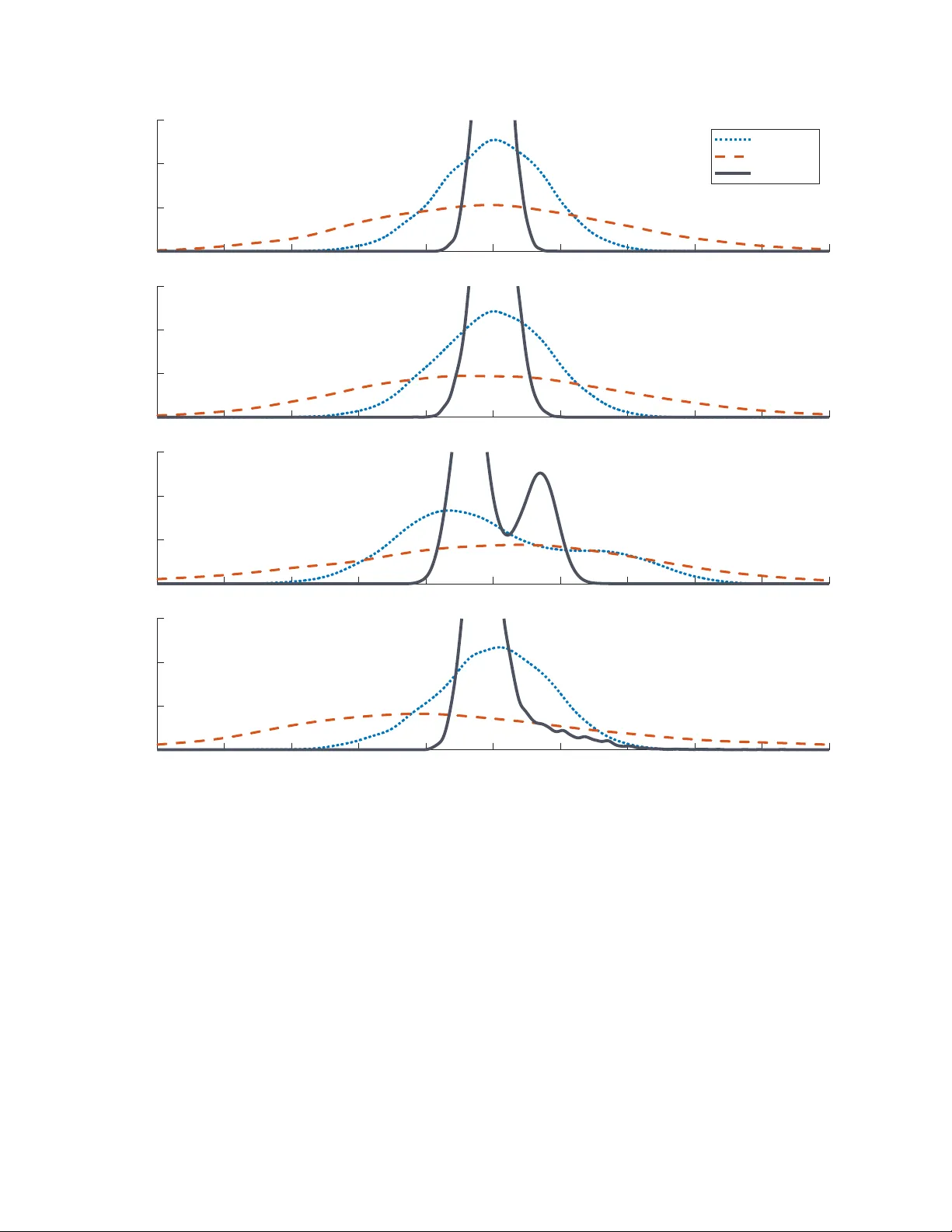
The Long Shado w of P andemic: Understanding the lingering eﬀects of cause-sp eciﬁc mortalit y sho c ks Y anxin Liu 1 and Kenneth Q. Zhou 2 ∗ 1 Departmen t of Finance, Universit y of Nebrask a-Lincoln, USA 2 Departmen t of Statistics and Actuarial Science, Universit y of W aterloo, Canada Marc h 24, 2026 Abstract: In the aftermath of the CO VID-19 pandemic, empirical data hav e revealed that large-scale health crises not only cause immediate disruptions in mortalit y dynamics but also hav e persistent eﬀects that ma y last for several y ears. Existing mortality models largely assume that mortalit y sho c ks are transitory and o verlook ho w their eﬀects can be long-lasting and heterogeneous across age groups and causes of death. In resp onse to this limitation, w e prop ose a nov el sto c hastic mortality mo del that captures age- and cause- sp eciﬁc long-lasting eﬀects of mortality jumps through a gamma-density-lik e decay function, estimated via a customized conditional maximum likelihoo d algorithm. Applying the mo del to recent U.S. mortality data, w e reveal divergen t persistence patterns across demographic groups and pro vide k ey insigh ts into the tail risk proﬁles of life insurance and ann uit y pro ducts. Our scenario-based analyses further show that neglecting p ersisten t shock eﬀects can lead to suboptimal hedging, while the proposed mo del enables what-if testing to analyze such eﬀects under p oten tial future health crises. Keywor ds: Mortality sho cks, L ong-lasting p andemic eﬀe cts, Sto chastic mortality mo deling, Cause-sp e ciﬁc mortality, Natur al he dging 1 In tro duction The COVID-19 pandemic has placed unpreceden ted ﬁnancial strain on the insurance industry , with higher- than-exp ected claims due to increased mortalit y , particularly during pandemic p eaks (Swiss Re, 2024). Life insurers face additional uncertain t y from v olatile p ost-pandemic mortalit y patterns, long CO VID’s eﬀects on future morbidity , and persistent behavioral and lifestyle changes, all of which complicate the assessment of long-term ﬁnancial obligations (Ng, 2021). These challenges ha ve forced insurers to reassess mortalit y assumptions and risk management strategies for handling future mortalit y shocks. Adv anced mortality mo dels that capture age-sp eciﬁc and cause-sp eciﬁc jump eﬀects in mortality trends are therefore essential for improv ed risk assessment and p ortfolio managemen t. Mo deling cause-sp eciﬁc mortalit y dynamics has drawn considerable in terest in industry , especially in the w ake of COVID-19. Recen t technical rep orts, such as Paglino et al. (2024) and Stryker (2025), sho w that the pandemic’s impact on mortalit y is highly heterogeneous across causes of death and age groups. F or older populations, CO VID-19 deaths accoun t for the ma jority of excess mortalit y , with non-CO VID causes playing a comparativ ely smaller role. By con trast, y ounger individuals’ non-CO VID excess deaths, ∗ Corresp onding author. E-mail: kenneth.zhou@uwaterlo o.c a 1 suc h as drug ov erdoses and vehicle accidents, constitute a substan tial share of total excess mortality . These disparities highligh t the imp ortance of incorp orating age-sp eciﬁc and cause-sp eciﬁc mortalit y dynamics in mo dels in tended to capture pandemic-related mortalit y sho c ks. The COVID-19 pandemic further reveals the complex interpla y of age-sp eciﬁc disparities, cause-sp eciﬁc patterns, and long-lasting/lingering eﬀects of mortalit y sho c ks. F or instance, respiratory diseases generally exhibited low er-than-exp ected mortality , cardiov ascular diseases sho wed p ersistent excess mortality , and ex- ternal causes suc h as acciden ts and substance use remained elev ated throughout the pandemic p erio d (Paglino et al., 2024; International Actuarial Association, 2021). Moreo v er, recen t data indicate that pandemic-related mortalit y eﬀects extend b ey ond the acute crisis phase, driven by factors such as long COVID complications, dela yed or foregone medical care, and lasting behavioral and so cioeconomic c hanges (P aglino et al., 2024; Swiss Re, 2024). These eﬀects collectiv ely generate intricate mortalit y dynamics that con v entional models struggle to capture. Sev eral studies hav e explored age- and cause-speciﬁc eﬀects to better understand mortalit y dynamics, with early contributions including Arnold and Sherris (2013); Alai et al. (2015); Arnold and Sherris (2015); Boumezoued et al. (2018); Alai et al. (2018). Building on this foundation, Li and Lu (2019) employ hi- erarc hical Arc himedean copulas to model cause-sp eciﬁc mortalit y . Li et al. (2019) introduce a forecast reconciliation approach for capturing cause-sp eciﬁc mortality eﬀects across diﬀerent age groups and p opula- tions, while Arnold and Glushk o (2022) use cointegration analysis within a vector error-correction mo del to analyze cause-sp eciﬁc mortalit y trends. More recen tly , a range of additional features, including elimination eﬀects and so cio economic factors, hav e been studied by Huynh and Ludk o vski (2024); Yiu et al. (2023, 2024); Dong et al. (2025); V arga (2025); T anak a and Matsuyama (2025); Villegas et al. (2025); Graziani and Nigri (2025). This gro wing b o dy of research underscores the imp ortance of isolating the causes of death and age eﬀects for improv ed mortality forecasting and risk assessmen t. Prior to the COVID-19 pandemic, a n um b er of sto chastic mortality mo dels with jump eﬀects were dev elop ed to understand extreme mortality risk. In a con tinuous-time setting, Biﬃs (2005) and Hainaut and Dev older (2008) emplo y jump-diﬀusion and L´ evy-pro cess sp eciﬁcations to c haracterize mortality jump eﬀects. In a discrete-time setting, some researchers consider permanent jumps in whic h extreme ev en ts aﬀect mortalit y dynamics indeﬁnitely (Cox et al., 2006, 2010; Arık et al., 2023), while others emphasize short-term transitory eﬀects (Chen and Cox, 2009; Lin et al., 2013; Liu and Li, 2015; ¨ Ozen and S ¸ ahin, 2020). Regarding the distribution of jump o ccurrence, Chen and Co x (2009) assume independent Bernoulli distributions, whereas Cox et al. (2006) consider Poisson jump counts. F or the severit y of jump eﬀects, several researchers use a normal distribution (Chen and Co x, 2009; Liu and Li, 2015), while double-exp onen tial jumps are used b y Deng et al. (2012) and Chen (2014), and extreme v alue theory is applied by Chen and Cummins (2010). Since the COVID-19 pandemic, extensiv e research has b een conducted on mortality modeling with pandemic-related eﬀects. Zhou and Li (2022) prop ose a three-parameter-lev el Lee-Carter extension to sim- ulate future mortalit y scenarios with COVID-lik e eﬀects. Chen et al. (2022) in tro duce a threshold jump framew ork, while Carannante et al. (2022) analyze the eﬀect of accelerated mortality sho c ks on life insur- ance contracts. Robben et al. (2022) and Sc hn ¨ urc h et al. (2022) study how pandemic data alter the calibration and pro jection of stochastic mortalit y mo dels, and Robben and Antonio (2024) extend this line of work to a multi-population setting. v an Berkum et al. (2025) extend the Li-Lee model with a third pandemic lay er calibrated to w eekly mortality data, while Go es et al. (2025) extend the Lee-Carter mo del b y introducing Ba yesian mortalit y mo dels with “v anishing” jump eﬀects, where pandemic sho cks are represen ted by serially dep enden t jump comp onents. 2 Motiv ated by the empirical evidence and recen t ﬁndings, this pap er develops a no vel stochastic mortalit y mo del that sim ultaneously captures age-sp eciﬁc sev erity , cause-speciﬁc patterns, and long-lasting p ersistence in mortality sho cks. Unlike most existing mo dels that treat jumps as either purely transitory or p ermanen t, our approac h introduces a ﬂexible deca y structure that allo ws sho c k eﬀects to ev olve diﬀeren tly across causes of death. The mo del is designed to serv e practical applications in life insurance risk managemen t, including liabilit y v aluation, de-risking strategies, and scenario-based stress testing. By providing a ﬂexible mo deling framew ork with empirically grounded features, this researc h equips actuaries and risk managers with tools for robust mortality risk assessment and long-term liability management. The metho dological con tribution of this paper is a three-wa y parallel factors mo del with cause-speciﬁc lingering jump eﬀects. The mo del decomposes log mortalit y rates into common trends, cause-sp eciﬁc devi- ations, and a no vel jump comp onen t that captures b oth age-speciﬁc severit y and cause-sp eciﬁc p ersistence through a gamma-densit y-lik e deca y function. Applied to U.S. male mortality data spanning 1968–2023, the mo del reveals divergen t pandemic impacts, such as causes with high initial severit y but rapid decay and causes with low er sev erity but prolonged p ersistence. W e also develop a conditional maxim um likelihoo d estimation approac h that eﬃcien tly handles the model’s complexity while preserving estimation accuracy . Robustness chec ks conﬁrm that the jump comp onen t successfully isolates pandemic eﬀects without distort- ing long-term mortalit y trends, and model comparisons demonstrate the necessity of incorporating b oth age-sp eciﬁc and cause-sp eciﬁc heterogeneity . Bey ond its metho dological contribution, the mo del oﬀers practical insigh ts for life insurance risk man- agemen t. W e examine natural hedging of longevity risk b y balancing life insurance and ann uity pro ducts in p ortfolio construction. The analysis rev eals that optimal hedging requires accurate mo deling of both age-sp eciﬁc and cause-sp eciﬁc mortality dynamics. Models that aggregate across causes or ages produce missp eciﬁed hedge ratios, substan tially increasing p ortfolio risk relativ e to the optimal hedge. Scenario analyses demonstrate the mo del’s ﬂexibilit y in ev aluating div erse mortalit y futures, including permanent mortalit y improv ements from medical breakthroughs, endemic regimes with frequent mild shocks, and catas- trophic even ts concen trated in speciﬁc age ranges. These capabilities provide insurers with to ols for robust long-term risk planning under mortality uncertaint y . The remainder of this paper is organized as follows. Section 2 describ es the cause-s peciﬁc mortality data and presen ts empirical evidence of heterogeneous and long-lasting pandemic eﬀects across age groups and causes of death. Section 3 introduces the 3WPF-CLJ model with its cause-sp eciﬁc lingering jump structure. Section 4 presents the estimation results and analyzes parameter estimates, robustness, and mo del comparisons. Section 5 examines applications to natural hedging and what-if scenario analysis for life insurance risk management. Lastly , Section 6 concludes. 2 Data and Motiv ation In this section, w e pro vide empirical evidence motiv ating the dev elopment of age- and cause-sp eciﬁc mortality mo dels capable of capturing long-lasting pandemic eﬀects. W e begin by describing the mortality data used throughout this study . W e then in vestigate the pandemic’s impact on aggregate mortality trends and the heterogeneit y across age groups and causes of death. Lastly , we analyze the p ersistence of pandemic mortality sho c ks ov er the p ost-pandemic years. 3 2.1 Data Description This pap er utilizes mortality data from the U.S. Centers for Disease Control and Preven tion (CDC) W ON- DER system. † The dataset includes male and female mortality rates disaggregated by age group, year, and cause of death (CoD), obtained from tw o primary sources. The Compr esse d Mortality Dataset pro vides death counts and population estimates from 1968 to 2016, spanning three revisions of the International Classiﬁcation of Diseases (ICD) co ding system: ICD-8 (1968–1978), ICD-9 (1979–1998), and ICD-10 (1999– 2016). The Underlying Cause of De ath Dataset extends cov erage from 1999 to 2023 using ICD-10 co des, with bridged-race categories for 1999–2020 and single-race categories for 2018–2023. W e combine these sources b y using the Compressed Mortality Dataset for 1968–1998 and the Underlying Cause of Death Dataset for 1999–2023, yielding a uniﬁed sample of 56 y ears (1968–2023) across 13 age groups (0–1, 1–4, 5–9, 10–14, 15–19, 20–24, 25–34, 35–44, 45–54, 55–64, 65–74, 75–84, and 85+). F ollowing Arnold and Glushk o (2022), w e classify deaths in to six CoD groups, with the ﬁrst ﬁv e corresponding to ma jor disease categories and the sixth capturing all remaining causes including COVID-19, as summarized in T able 1. W e let D x,t,c denote the num b er of deaths for age group x in y ear t due to cause c . This quantit y is structured as a three-dimensional array with dimensions 13 × 56 × 6. W e let E x,t denote the population exp osures for age group x in year t . Note that E x,t remains constant across CoD groups for a given age-year combination, and therefore is structured as a tw o-dimensional arra y with dimensions 13 × 56. The mortality rate for a sp eciﬁc CoD group c is then deﬁned as m x,t,c = D x,t,c /E x,t , which serves as the primary quantit y of interest in the remainder of this paper. Co ding system ICD-10 Co ding ICD-9 Co ding ICD-8 Co ding P erio d 1999–2023 1979–1998 1968–1978 CoD 1: Infectious Diseases A00-B99 001-139 001-136 CoD 2: Cancer C00-D48 140-239 140-239 CoD 3: Circulatory Diseases I00-I99 390-437 390-458 CoD 4: Respiratory Diseases J00-J98 460-519 460-519 CoD 5: External Causes V00-Y89 E800-E999 E810-E999 CoD 6: Other Causes + CO VID All other causes (including CO VID-19) T able 1: Summary of cause of death groupings across ICD co ding systems. 2.2 Mortalit y T rends Figure 1 presents the p erio d life exp ectancy at age 35 from 1995 to 2023 for U.S. males and females, along with y ear-o ver-y ear changes in life exp ectancy sho wn on the righ t y-axis. T o calculate these life expectancies, w e apply spline interpolation to the log mortality rates ln( m x,t,c ) along the age dimension for each cause and y ear, whic h preserves the age-sp eciﬁc patterns inheren t to eac h cause and y ear. The p erio d life exp ectancy for each year is then obtained b y com bining mortality across all causes of death. Leading up to the CO VID-19 pandemic, life exp ectancy exhibited a steady up ward trend before 2010, fol- lo wed by a perio d of stalled impro vemen t up to 2019. Life exp ectancy at age 35 increased from appro ximately † The CDC WONDER system: https://wonder.cdc.gov 4 Y ear 1995 2000 2005 2010 2015 2020 Life Expectancy at Age 35 40 41 42 43 44 45 46 47 48 Change in Life Expectancy (Y ears) -2.5 -2 -1.5 -1 -0.5 0 0.5 1 1.5 2 2.5 Male Y ear 1995 2000 2005 2010 2015 2020 Life Expectancy at Age 35 40 41 42 43 44 45 46 47 48 Change in Life Expectancy (Y ears) -2.5 -2 -1.5 -1 -0.5 0 0.5 1 1.5 2 2.5 Female Figure 1: P erio d life exp ectancy at age 35 (dotted line) and y ear-ov er-year changes (v ertical bars) for U.S. males and females, 1995–2023, with highlighted mark ers indicating the CO VID-19 pandemic p eriod. 40 y ears in 1995 to around 43.5 years by 2010 for males, and then remained largely ﬂat until 2019. F emales sho wed a similar pattern, with life expectancy rising from ab out 45.5 y ears in 1995 to appro ximately 47 y ears b y 2010, and then plateauing through 2019. In 2020, a sharp decline disrupted this tra jectory , marking the immediate and profound impact of the COVID-19 pandemic. The situation deteriorated further in 2021 as the pandemic contin ued. The year-o ver-y ear changes reveal that life exp ectancy decreased by approximately 2–2.5 years during the peak pandemic years for b oth males and females. In 2022 and 2023, mild reco v eries in life e xpectancy were observed. Nevertheless, life exp ectancy at age 35 remained w ell b elo w pre-pandemic lev els, highlighting the pandemic’s enduring eﬀects on aggregated mortalit y trends. 2.3 Heterogeneit y b y Age and Cause W e no w in vestigate how the pandemic’s impact v aried across age groups and causes of death. Figure 2 presen ts the p ercen tage c hange in mortalit y rates b et w een 2019 and 2020 across 13 age groups and 6 causes of death for b oth males and females. The color intensit y indicates the magnitude and direction of c hange, with red represen ting increases in mortality and blue representing decreases. Numerical v alues display ed in eac h cell pro vide precise p ercen tage changes for detailed comparison across age groups and causes. The heatmap reveals substantial heterogeneit y in the initial pandemic impact across age groups and causes. CoD 6 (Other + COVID) exhibited the most dramatic increases across nearly all age groups, with p ercen tage changes ranging from approximately 40% to 70% for individuals aged 25 and older. This pattern is consistent across b oth genders and reﬂects the direct mortality burden of COVID-19. In con trast, CoD 1 (Infectious) sho wed clear decreases among younger age groups, with reductions reaching 20% to 40% for ages under 15, and young females e xperiencing stronger decreases than young males. CoD 5 (External) display ed notable increases concentrated in teenage and working-age groups (10–64 years), with changes ranging from 10% to 25%, and the impact w as more pronounced for males than females. F or the remaining causes of death, the pandemic’s initial impact was relatively mo dest. CoD 2 (Cancer) 5 Infectious Cancer Circulatory Respiratory External Other + COVID Cause of Death 85+ 75-84 65-74 55-64 45-54 35-44 25-34 20-24 15-19 10-14 5-9 1-4 <1 Age Group Male -0.9 2.2 7.7 5.5 7.0 14.3 5.0 -0.6 4.7 -18.7 -24.6 -28.8 -16.8 -1.2 -2.0 -0.8 -1.5 -2.4 2.5 -2.7 -5.4 -8.2 -1.5 7.1 -1.3 -4.8 1.4 3.4 6.4 10.7 1 1.5 15.1 13.2 3.8 1 1.9 19.4 -22.1 -10.1 -14.2 -5.5 -1.6 2.0 7.0 13.0 23.1 18.9 9.8 -0.4 3.0 -15.6 -24.0 -28.1 1.8 -1.9 3.0 9.0 15.4 20.3 23.3 22.9 26.2 18.7 -1.0 1 1.5 -7.3 50.3 66.5 77.0 67.4 67.5 66.6 53.6 39.7 13.1 6.6 -4.4 -1.8 -4.4 -60 -40 -20 0 20 40 60 Infectious Cancer Circulatory Respiratory External Other + COVID Cause of Death 85+ 75-84 65-74 55-64 45-54 35-44 25-34 20-24 15-19 10-14 5-9 1-4 <1 Age Group Female -0.6 1.7 6.9 8.8 12.6 13.9 -4.2 14.6 3.7 -48.3 -39.7 -43.1 -30.3 -2.9 -0.9 -0.6 -0.8 -0.9 -2.8 2.8 -4.6 -2.4 1.2 -3.7 9.9 -1.0 1.7 2.3 6.9 8.2 1 1.7 12.3 1 1.9 1.0 7.9 7.1 -31.9 -4.4 9.6 -8.1 -4.3 -2.7 3.6 5.1 14.7 6.1 7.8 21.9 -6.0 -1 1.8 -18.6 -25.2 1.5 -1.4 0.2 8.2 9.8 20.9 21.3 19.9 16.9 12.7 -1.0 -4.4 -3.4 41.4 50.2 62.6 57.1 54.9 47.3 38.4 23.2 21.6 -9.4 -6.6 -6.1 -3.7 -60 -40 -20 0 20 40 60 Figure 2: Percen tage c hange in mortality rates from 2019 to 2020 b y age group and cause of death for U.S. males (left) and females (righ t). sho wed minimal changes across most age groups, with percentage changes t ypically within ± 5%. CoD 3 (Circulatory) and CoD 4 (Respiratory) exhibited mixed patterns, with sligh t decreases among y ounger ages and mo dest increases among older ages. These heterogeneous patterns rev eal that the pandemic represen ts more than just an additional cause of death but rather a systematic and diﬀerential sho ck to pre-existing mortalit y dynamics. This complexity underscores the need for developing age- and cause-speciﬁc mo deling framew orks capable of capturing suc h heterogeneous mortality sho c ks. 2.4 Evidence of Long-Lasting Eﬀects Bey ond the heterogeneous initial impact across age groups and causes, w e also inv estigate whether the recen t pandemic mortality sho cks hav e long-lasting eﬀects ov er m ultiple years, particularly fo cusing on the diﬀerences among causes of death. T o quantify the long-lasting eﬀects, we examine excess log mortalit y rates in the p ost-pandemic years, deﬁned as E M x,t,c = ln( m x,t,c ) − ln( m x,t ∗ ,c ) , where t ∗ is ﬁxed at 2019 as the baseline y ear immediately prior to the pandemic, and t ranges from 2020 to 2023. Figure 3 presents the distribution of E M x,t,c for each cause during years 2020–2023. Each panel displa ys b ox plots of E M x,t,c across age groups, while the blac k dots indicate the age-standardized mean. A cubic spline curve is used to illustrate the tra jectory of the age-standardized rates ov er time. Figure 3 reveals that p ersistence patterns diﬀer substantially across the 6 causes of death. CoD 6 (Other + COVID) demonstrates the largest initial surge in 2020, p eaking in 2021 and sharply declining afterw ard. CoD 3 (Circulatory) and CoD 5 (External) show more p ersisten t eﬀects, reac hing their p eak in 2021–2022 and exp eriencing slow er decay afterward. CoD 1 (Infectious), CoD 2 (Cancer), and CoD 4 (Respiratory) displa y 6 Y ear 2020 2021 2022 2023 Excess Log Mortality Rate -0.4 -0.2 0 0.2 0.4 CoD 1: Infectious Y ear 2020 2021 2022 2023 Excess Log Mortality Rate -0.15 -0.1 -0.05 0 0.05 0.1 CoD 2: Cancer Y ear 2020 2021 2022 2023 Excess Log Mortality Rate -0.1 0 0.1 0.2 CoD 3: Circulatory Y ear 2020 2021 2022 2023 Excess Log Mortality Rate -0.4 -0.2 0 0.2 CoD 4: Respiratory Y ear 2020 2021 2022 2023 Excess Log Mortality Rate -0.1 0 0.1 0.2 0.3 CoD 5: External Y ear 2020 2021 2022 2023 Excess Log Mortality Rate 0 0.2 0.4 0.6 0.8 CoD 6: Other + COVID Figure 3: Excess log mortality rates in y ears 2020–2023 by cause of death for U.S. males; box plots sho w age distributions, dots sho w age-standardized means, and splines sho w temp oral tra jectories. 7 minimal ﬂuctuations near zero throughout the perio d. These div ergent patterns indicate that pandemic mortalit y sho cks v ary substantially in their p ersistence across causes of death. 3 The Prop osed Mo del This section introduces our three-w ay parallel factors model with cause-speciﬁc long-lasting/lingering mor- talit y jump eﬀects (3WPF-CLJ model). Motiv ated by the empirical ﬁndings from Section 2, we dev elop a sto c hastic mortality mo del that captures age- and cause-sp eciﬁc jump eﬀects with heterogeneous p ersistence patterns. W e ﬁrst presen t the model structure and distributional assumptions, and then deriv e an estimation approac h tailored to the model along with the likelihoo d function based on mortalit y improv ement rates. 3.1 Mo del Structure The prop osed 3WPF-CLJ mo del decomp oses the log mortality rate as follows: ln( m x,t,c ) = a x,c + B x K t + φ c b x k t + N t J ( τ ) x,c + e x,t,c . (1) In this decomposition, the ﬁrst component a x,c represen ts the lev el of mortalit y rate at age x for cause of death (CoD) c . The second comp onent is the pro duct of B x and K t , which represen ts the common factor shared by all causes of death. In particular, K t captures the v ariation of log mortality rates ov er time, and B x measures the sensitivity of log mortalit y rates to changes in K t . The third comp onent is the product of φ c , b x , and k t , which reﬂects the long-term cause-speciﬁc deviation from the general trend in the cause of death, age, and time dimensions, resp ectiv ely . The fourth comp onen t N t J ( τ ) x,c captures the jump eﬀects, whic h we discuss in detail below. Finally , the ﬁfth comp onent e x,t,c is the error term. The ma jor nov elt y of the prop osed mo del is the fourth comp onen t N t J ( τ ) x,c , which captures the hetero- geneous jump eﬀects. W e let N t = 1 { t ≥ T J } b e an indicator v ariable, where T J is the year of pandemic o ccurrence, with N t = 1 meaning that a jump has o ccurred on or b efore year t , and N t = 0, otherwise. W e let J ( τ ) x,c b e the lingering jump v ariable at age x attributed to cause of death c . The sup erscript τ denotes the time elapsed since the jump o ccurrence, computed as τ = t − T J . W e then deﬁne the cause-sp eciﬁc lingering jump eﬀect by J ( τ ) x,c =      0 , τ < 0 or equiv alently , t < T J J x,c , τ = 0 or equiv alently , t = T J J x,c × π c ( τ ) , τ > 0 or equiv alently , t > T J (2) where J x,c represen ts the size of the initial jump for age x attributed to cause of death c , and π c ( τ ) represen ts the long-lasting eﬀect for cause of death c . W e remark that J ( τ ) x,c can capture the follo wing three scenarios: 1. Prior to jump o ccurrence ( t < T J ), there is no jump eﬀect to capture. 2. When the jump o ccurs ( t = T J ), the initial impact is captured b y J x,c . 3. After jump occurrence ( t > T J ), the long-lasting eﬀect is captured by π c ( τ ), a parametric function of time elapsed τ . T o incorp orate the cause-speciﬁc long-lasting eﬀects illustrated in Figure 3, we deﬁne π c ( τ ) = γ c × β α c c × τ α c − 1 × e − β c τ , (3) 8 for τ > 0, with magnitude parameter γ c , shape parameter α c , and rate parameter β c that are all cause- sp eciﬁc. The magnitude parameter γ c supplemen ts J x,c to adjust the size of the lingering jump eﬀect. The shap e parameter α c con trols the timing of the p eak eﬀect, allowing diﬀerent causes of death to hav e v arying resp onse patterns to the same extreme mortality even t. The rate parameter β c determines how rapidly the jump eﬀect decays. It is w orth noting that the speciﬁcation of π c ( τ ) is identical to a gamma density with parameters α c and β c , scaled by the magnitude parameter γ c . Equation (2) can b e compactly expressed as J ( τ ) x,c = J x,c × π c ( τ ) , (4) where π c ( τ ) = 0 when τ < 0, and π c ( τ ) = 1 when τ = 0. W e conclude this subsection b y highligh ting sev eral key features of the prop osed 3WPF-CLJ mo del. First, follo wing the spirit of the Li-Lee mo del dev elop ed b y Li and Lee (2005), the 3WPF-CLJ model incorp orates b oth a common factor and a cause-sp eciﬁc factor. This design allo ws us to capture the general mortalit y trend while preserving the distinct features associated with diﬀerent causes of death. Second, inspired by the three-wa y Lee-Carter mo del developed b y Russolillo et al. (2011) and the four-w ay structure considered in Cardillo et al. (2023), our mo del uses a single compact comp onent φ c b x k t to capture the cause- sp eciﬁc deviation from the general trend. Finally , the 3WPF-CLJ mo del extends the transitory jump models in tro duced in Liu and Li (2015) b y replacing J x,t with J ( τ ) x,c . This extension allows the mo del to account not only for age-sp eciﬁc mortality jumps but also for long-lasting cause-speciﬁc eﬀects. 3.2 Mo del Assumptions W e now pro vide the distributional assumptions underlying the prop osed mo del. • The p erio d eﬀect for the general trend K t follo ws a random walk with drift D : K t = D + K t − 1 + η t where η t ∼ N  0 , σ 2 η  . This assumption is widely adopted in sto c hastic mortality mo deling, including the original Lee-Carter model (Lee and Carter, 1992) and the Li-Lee mo del (Li and Lee, 2005). • The p erio d eﬀect for the cause-sp eciﬁc trend k t also follows a random walk with drift d : k t = d + k t − 1 + ξ t where ξ t ∼ N  0 , σ 2 ξ  . F or simplicity , w e assume η t and ξ t are uncorrelated. • The o ccurrence of a jump in eac h y ear follo ws an independent Bernoulli distribution; that is, N t ∼ Bern( p ), where p denotes the probability of a jump o ccurring in a given year. W e assume at most one jump o ccurs within the sample p erio d. ‡ Under this assumption, the jump occurrence time T J follo ws a geometric distribution with probability mass function P ( T J = t J ) = P ( N 1 = · · · = N t J − 1 = 0 , N t J = · · · = N T = 1) = (1 − p ) t J − 1 × p. When no jump occurs, we hav e P ( T J  = 1 , . . . , T ) = P ( N 1 = · · · = N T = 0) = (1 − p ) T . ‡ This assumption is appropriate for our dataset, whic h spans 1968–2023 and con tains only one ma jor extreme mortalit y even t (COVID-19). It allows us to fo cus on characterizing the long-lasting eﬀects of this pandemic. 9 • The severit y of the initial jump eﬀect J x,c follo ws a normal distribution with mean v arying across ages and causes of death. Due to the limited num b er of realized jumps in our dataset, w e assume constant v ariance across all age-cause com binations. W e denote the mean and v ariance b y µ x,c := E ( J x,c ) and σ 2 J := V ar ( J x,c ) . Under this sp eciﬁcation, the expectation and v ariance of the lingering jump eﬀect J ( τ ) x,c are given by E  J ( τ ) x,c  = µ x,c × π c ( τ ) (5) and V ar  J ( τ ) x,c  = σ 2 J × ( π c ( τ )) 2 , (6) resp ectiv ely . • The error term e x,t,c follo ws a normal distribution with ze ro mean and constan t v ariance; that is, e x,t,c ∼ N (0 , σ 2 e ). 3.3 Mo del Estimation W e conduct parameter estimation using the Route I I estimation metho d, which has b een shown to p erform w ell for Lee-Carter t yp e mo dels (Hab erman and Renshaw, 2012) and has b een implemented in mortalit y mo dels with transitory jump eﬀects (Liu and Li, 2015). Under the assumptions outlined in Section 3.2, the Route I I approach can eﬀectiv ely reduce the num b er of parameters needed for estimation. 3.3.1 Deﬁning Mortality Impro vemen t Rates T o implement the Route I I estimation method, we ﬁrst introduce the notation Z x,t,c := ln( m x,t,c ) − ln( m x,t − 1 ,c ) to represen t the log mortality impro v ement rate at age x in y ear t for cause of death c . T aking the ﬁrst diﬀerence of equation (1), we obtain Z x,t,c = B x ( K t − K t − 1 ) + φ c b x ( k t − k t − 1 ) + N t J ( τ ) x,c − N t − 1 J ( τ − 1) x,c + e x,t,c − e x,t − 1 ,c , whic h, under the random w alk assumptions on K t and k t , simpliﬁes to Z x,t,c = B x ( D + η t ) + φ c b x ( d + ξ t ) + N t J ( τ ) x,c − N t − 1 J ( τ − 1) x,c + e x,t,c − e x,t − 1 ,c . (7) Conditional on N t − 1 and N t , Z x,t,c follo ws a normal distribution with mean equal to E( Z x,t,c | N t − 1 , N t ) = B x D + φ c b x d + ( N t π c ( τ ) − N t − 1 π c ( τ − 1)) µ x,c =      B x D + φ c b x d , N t − 1 = N t = 0 B x D + φ c b x d + µ x,c , N t − 1 = 0 , N t = 1 B x D + φ c b x d + ( π c ( τ ) − π c ( τ − 1)) × µ x,c , N t − 1 = N t = 1 (8) and v ariance equal to V ar( Z x,t,c | N t − 1 , N t ) = B 2 x σ 2 η + φ 2 c b 2 x σ 2 ξ + ( N t π c ( τ ) − N t − 1 π c ( τ − 1)) 2 σ 2 J + 2 σ 2 e =      B 2 x σ 2 η + φ 2 c b 2 x σ 2 ξ + 2 σ 2 e , N t − 1 = N t = 0 B 2 x σ 2 η + φ 2 c b 2 x σ 2 ξ + σ 2 J + 2 σ 2 e , N t − 1 = 0 , N t = 1 B 2 x σ 2 η + φ 2 c b 2 x σ 2 ξ + ( π c ( τ ) − π c ( τ − 1)) 2 σ 2 J + 2 σ 2 e , N t − 1 = N t = 1 . (9) 10 Dep ending on the v alues of N t − 1 and N t , the conditional distribution of Z x,t,c corresp onds to one of three scenarios. The ﬁrst scenario is N t − 1 = N t = 0, whic h indicates that no jump has o ccurred and thus the jump eﬀect can be excluded from the mean and v ariance. In the second scenario, we ha v e N t − 1 = 0 and N t = 1, whic h indicate that a jump o ccurs in y ear t and the jump eﬀect enters the mo del but with no p ersistence yet. In the last scenario, N t − 1 = N t = 1 indicates that a jump o ccurred prior to year t and the long-lasting eﬀect of the jump needs to b e incorp orated into the mean and v ariance. 3.3.2 Designing a Matrix Represen tation The expressions in equations (7), (8), and (9) can be expressed compactly using a matrix representation. Because of the three-dimensional structure of our dataset, the log mortality impro vemen t rates are indexed b y age, time, and cause. W e suppress these three dimensions in to a matrix represen tation as follo ws. Suppressing the Age Dimension W e ﬁrst suppress the age dimension by using the notation  Z t,c =       Z 1 ,t,c Z 2 ,t,c . . . Z X,t,c       ,  J c =       J 1 ,c J 2 ,c . . . J X,c       ,  µ c =       µ 1 ,c µ 2 ,c . . . µ X,c       ,  e t,c =       e 1 ,t,c e 2 ,t,c . . . e X,t,c       to represent vectors of log mortality impro v ement rates, jump eﬀects, exp ected jump eﬀects, and errors in y ear t for the cause of death c , and  B = ( B 1 , B 2 , . . . , B X ) ⊤ ,  b = ( b 1 , b 2 , . . . , b X ) ⊤ ,  1 X = (1 , 1 , . . . , 1) ⊤ to represent v ectors of B x , b x , and ones with X elements, resp ectiv ely . The v ector of lingering jump eﬀects in year t for cause of death c is then given b y  J ( τ ) c =  J c × π c ( τ ). It follows that equation (7) can b e expressed as  Z t,c =  B ( D + η t ) + φ c  b ( d + ξ t ) + N t  J ( τ ) c − N t − 1  J ( τ − 1) c +  e t,c −  e t − 1 ,c . Suppressing the Cause Dimension Pro ceeding similarly , we suppress the cause dimension by using  Z t =        Z t, 1  Z t, 2 . . .  Z t,C       ,  J =        J 1  J 2 . . .  J C       ,  µ =        µ 1  µ 2 . . .  µ C       ,  e t =        e t, 1  e t, 2 . . .  e t,C       to represent vectors of Z x,t,c , J x,c , E( J x,c ), and e x,t,c in year t , and  φ = ( φ 1 , φ 2 , . . . , φ C ) ⊤ ,  π ( τ ) = ( π 1 ( τ ) , π 2 ( τ ) , . . . , π C ( τ )) ⊤ ,  1 C = (1 , 1 , . . . , 1) ⊤ to represent vectors of φ c , π c ( τ ), and ones with C elements, resp ectiv ely . The lingering jump eﬀect in y ear t can b e expressed as  J ( τ ) =   π ( τ ) ⊗  1 X  ◦  J , 11 where ◦ denotes element-wise multiplication. The vector of log mortalit y impro vemen t rates in year t then follo ws  Z t =  1 C ⊗  B × ( D + η t ) +  φ ⊗  b × ( d + ξ t ) + N t  J ( τ ) − N t − 1  J ( τ − 1) +  e t −  e t − 1 =  1 C ⊗  B × ( D + η t ) +  φ ⊗  b × ( d + ξ t ) +  ( N t  π ( τ ) − N t − 1  π ( τ − 1)) ⊗  1 X  ◦  J +  e t −  e t − 1 , whic h provides a compact matrix representation of equation (7). Conditional on N t − 1 and N t ,  Z t follo ws a m ultiv ariate normal distribution with mean E   Z t | N t − 1 , N t  =  1 C ⊗  B × D +  φ ⊗  b × d +  ( N t  π ( τ ) − N t − 1  π ( τ − 1)) ⊗  1 X  ◦  µ and v ariance-cov ariance matrix V ar   Z t | N t − 1 , N t  =   1 C ⊗  B    1 C ⊗  B  ⊤ × σ 2 η +   φ ⊗  b    φ ⊗  b  ⊤ × σ 2 ξ + L t Σ J L ⊤ t + 2 × I X C × σ 2 e , where Σ J = I X C × σ 2 J b y deﬁnition, and L t is an ( X C )-by-( X C ) diagonal matrix with diagonal elements ( N t  π ( τ ) − N t − 1  π ( τ − 1)) ⊗  1 X and zeros elsewhere. Suppressing the Time Dimension Finally , we sp ecify the full vector of log mortality improv ement rates,  Z , by suppressing the time dimension. W e deﬁne  Z =        Z 2  Z 3 . . .  Z T       ,  η =       η 2 η 3 . . . η T       ,  ξ =       ξ 2 ξ 3 . . . ξ T       ,  N =       N 1 N 2 . . . N T       ,  π =        π (1 − t J )  π (2 − t J ) . . .  π ( T − t J )       ,  e =        e 1  e 2 . . .  e T       . The full vector of log mortality impro vemen t rates can be expressed as  Z = ( D ×  1 T − 1 +  η ) ⊗  1 C ⊗  B + ( d ×  1 T − 1 +  ξ ) ⊗  φ ⊗  b +  I ∗ C  (  N ⊗  1 C ) ◦  π  ⊗  1 X  ◦   1 T − 1 ⊗  J  + I ∗ X C  e, where I ∗ C =       − I C I C 0 · · · 0 0 0 − I C I C · · · 0 0 . . . . . . . . . . . . . . . . . . 0 0 · · · · · · − I C I C       is a sparse blo c k matrix with ( T − 1) rows and T columns of blocks, where each block I C is a C -by- C identit y matrix. Similarly , I ∗ X C is a sparse blo ck matrix with blo c ks I X C , where I X C is an X C -b y- X C identit y matrix. Conditional on  N , one can show that the exp ectation and v ariance of  Z are given by E(  Z |  N ) = ( D ×  1 T − 1 ) ⊗  1 C ⊗  B + ( d ×  1 T − 1 ) ⊗  φ ⊗  b +  I ∗ C  (  N ⊗  1 C ) ◦  π  ⊗  1 X  ◦   1 T − 1 ⊗  µ  (10) and V ar(  Z |  N ) = Σ η ⊗  1 C  1 ⊤ C ⊗  B  B ⊤ + Σ ξ ⊗  φ  φ ⊤ ⊗  b  b ⊤ + L  (  1 T − 1  1 ⊤ T − 1 ) ⊗ Σ J  L ⊤ + I ∗ X C Σ e ( I ∗ X C ) ⊤ , (11) resp ectiv ely , where Σ η = I T − 1 × σ 2 η , Σ ξ = I T − 1 × σ 2 ξ , Σ e = I T × σ 2 e , and L is a diagonal matrix with diagonal elemen ts I ∗ C  (  N ⊗  1 C ) ◦  π  and zeros elsewhere. 12 3.3.3 Deriving the Log-Lik eliho o d F unction F or notational conv enience, we use  θ to represen t the vector of all parameters in the proposed mo del, comprising parameters associated with the general mortality dynamic (  B , D, σ η ), cause-speciﬁc mortalit y dynamic (  b, d, σ ξ ), lingering jump eﬀects (  µ, σ J ,  α,  β ,  γ , p ), and the random noise ( σ e ). The log-likelihoo d function under the Route II approac h is given b y l (  θ ) = ln  f   z ;  θ  . (12) By the law of total probabilit y , the density function f   z ;  θ  can b e expressed as a sum o ver all jump o ccurrence patterns: f   z ;  θ  = P  N f   z |  N ;  θ  × P (  N ) = f   z | N 1 = · · · = N T = 0 ;  θ  × P ( N 1 = · · · = N T = 0) + f   z | N 1 = · · · = N T − 1 = 0 , N T = 1 ;  θ  × P ( N 1 = · · · = N T − 1 = 0 , N T = 1) + · · · + f   z | N 1 = · · · = N T = 1 ;  θ  × P ( N 1 = · · · = N T = 1) . (13) Substituting the assumption on jump occurrence from Section 3.2, we get f   z ;  θ  = f   z | N 1 = · · · = N T = 0 ;  θ  × (1 − p ) T No Jump + f   z | N 1 = · · · = N T − 1 = 0 , N T = 1 ;  θ  × (1 − p ) T − 1 × p Jump in Y ear T + · · · . . . + f   z | N 1 = · · · = N T = 1 ;  θ  × p, Jump in Y ear 1 (14) Therefore, f   z ;  θ  can b e in terpreted as a Gaussian mixture mo del comprising diﬀeren t jump o ccurrence scenarios. The mean and v ariance of eac h conditional distribution are given by equations (10) and (11), resp ectiv ely . 4 Mo del Analysis This section presen ts comprehensiv e analyses of the prop osed 3WPF-CLJ model. W e ﬁrst present the esti- mation results obtained using the Bro yden-Fletcher-Goldfarb-Shanno (BFGS) algorithm, with implementa- tion details provided in App endix B. W e then examine the mo del’s robustness across diﬀeren t calibration windo ws, with particular fo cus on the inﬂuence of the data in COVID y ears. Finally , we conduct model comparisons to demonstrate the imp ortance of incorp orating long-lasting/lingering jump eﬀects and the necessit y of allo wing cause-speciﬁc heterogeneit y in jump eﬀects. 4.1 Estimation Results W e ﬁt the proposed 3WPF-CLJ mo del to U.S. male mortalit y data from 1968 to 2023, as describ ed in Section 2. Recall that our dataset comprises 13 age groups, 6 causes (with CO VID-19 deaths categorized in CoD 13 Age Group <1 1-4 5-9 10-14 15-19 20-24 25-34 35-44 45-54 55-64 65-74 75-84 85+ B x -0.05 0 0.05 0.1 0.15 0.2 Estimated V alue 95% Conﬁdence Interval Age Group <1 1-4 5-9 10-14 15-19 20-24 25-34 35-44 45-54 55-64 65-74 75-84 85+ b x -0.05 0 0.05 0.1 0.15 0.2 0.25 Figure 4: Estimated v alues of B x and b x with 95% conﬁdence interv als from the 3WPF-CLJ mo del ﬁtted to U.S. male mortalit y data from 1968 to 2023. 6), and 56 y ears of observ ations. The maximized log-likelihoo d function is 4 . 5422 × 10 3 , with 135 model parameters, yielding an AIC of − 8 . 8143 × 10 3 and a BIC of − 7 . 9552 × 10 3 . Figure 4 presents the estimated v alues and 95% conﬁdence interv als for the common age pattern B x and the cause-speciﬁc age deviations b x . The down ward-sloping pattern of B x in the left panel of Figure 4 reveals a negative correlation b etw een mortality impro vemen t and age, indicating that older individuals experience smaller mortalit y impro vemen ts than younger individuals. In con trast, the righ t panel of Figure 4 shows a mark edly diﬀeren t pattern for b x , resembling a mixture of tw o normal densities with p eaks at ages 10–14 and 25–34. Notably , the magnitude of φ 1 for CoD 1 (Infectious) is signiﬁcantly greater than that for the other CoDs (see T able 2). Consequen tly , the pattern of b x primarily captures deviations from CoD 1, which in our dataset is not related to the COVID-19 pandemic. Figure 5 presents the estimated jump sev erit y levels µ x,c and their 95% conﬁdence in terv als for the 6 causes of death. The div ergent patterns across panels reﬂect the asymmetric impact of CO VID-19 on diﬀeren t causes of death. Among the six CoDs, CoD 6 (Other + COVID) exhibits the highest sev erity level, with its age pattern of µ x, 6 consisten t with ﬁndings in Dong et al. (2020) showing that older individuals face higher CO VID-19 risk. In contrast, CoD 2 (Cancer) shows only mild pandemic eﬀects, with insigniﬁcant jump eﬀects across all age groups except infants. The remaining four CoDs exhibit v arying eﬀects across age groups. F or CoD 1 (Infectious) and CoD 4 (Respiratory), negative v alues app ear in y oung age groups, suggesting that mask regulations during COVID- 19 had a protectiv e impact on infectious and respiratory diseases for children. Notably , CoD 5 (External) sho ws p eak v alues concentrated at ages 15–44, indicating that CO VID-19 negatively aﬀected young and middle-aged adults through external causes of death. This outcome aligns with ﬁndings in Czeisler et al. (2020), where the pandemic and its asso ciated risk mitigation activities (such as so cial distancing and home- w orking environmen ts) p osed increasing challenges to mental health. Figure 6 presen ts the ﬁtted lingering jump eﬀects µ x,c × π c ( τ ) for the 6 causes of death across p ost- 14 <1 1-4 5-9 10-14 15-19 20-24 25-34 35-44 45-54 55-64 65-74 75-84 85+ 7 x;c -0.5 -0.3 -0.1 0.1 0.3 0.5 0.7 CoD 1: Infectious 95% Conﬁdence Interval Estimated V alue <1 1-4 5-9 10-14 15-19 20-24 25-34 35-44 45-54 55-64 65-74 75-84 85+ 7 x;c -0.5 -0.3 -0.1 0.1 0.3 0.5 0.7 CoD 2: Cancer <1 1-4 5-9 10-14 15-19 20-24 25-34 35-44 45-54 55-64 65-74 75-84 85+ 7 x;c -0.5 -0.3 -0.1 0.1 0.3 0.5 0.7 CoD 3: Circulatory Age Group <1 1-4 5-9 10-14 15-19 20-24 25-34 35-44 45-54 55-64 65-74 75-84 85+ 7 x;c -0.5 -0.3 -0.1 0.1 0.3 0.5 0.7 CoD 4: Respiratory Age Group <1 1-4 5-9 10-14 15-19 20-24 25-34 35-44 45-54 55-64 65-74 75-84 85+ 7 x;c -0.5 -0.3 -0.1 0.1 0.3 0.5 0.7 CoD 5: External Age Group <1 1-4 5-9 10-14 15-19 20-24 25-34 35-44 45-54 55-64 65-74 75-84 85+ 7 x;c -0.5 -0.3 -0.1 0.1 0.3 0.5 0.7 CoD 6: Other + COVID Figure 5: Estimated v alues of µ x,c with 95% conﬁdence interv als from the 3WPF-CLJ mo del ﬁtted to U.S. male mortalit y data from 1968 to 2023. pandemic y ears 2020–2023. The ﬁtted patterns align closely with the empirical observ ations from Figure 3. CoD 6 (Other + CO VID) exhibits the highest initial jump sev erity , with eﬀects deca ying rapidly ov er subsequen t y ears. In contrast, CoD 5 (External) displays smaller initial sev erity but more p ersisten t eﬀects. CoD 1 (Infectious) and CoD 4 (Respiratory) show negative jump eﬀects during the pandemic, though these b eneﬁts disapp ear within one y ear. Finally , CoD 2 (Cancer) and CoD 3 (Circulatory) exhibit only mo dest pandemic impacts with minimal lasting eﬀects. T able 2 summarizes the estimated v alues and standard errors for the remaining parameters in the 3WPF- CLJ model. W e note that extra caution should b e tak en when interpreting ln( σ J ) and logit( p ), since the cause-sp eciﬁc mortality data w e used do not cov er catastrophic mortalit y even ts other than the COVID-19 pandemic (e.g., the 1918 inﬂuenza pandemic, W orld W ar I, and W orld W ar I I). The jump severit y volatilit y σ J has a large standard error due to the limited num b er of statistically meaningful jumps. The jump probabilit y p is estimated at approximately 0 . 0188, suggesting that the mo del has detected only one jump from 56 years of observ ations. 15 Ti me La g ( = ) 1 2 3 4 5 6 Fitted Long-Lasting Jump Effect -0.2 -0.1 0 0.1 0.2 0.3 0.4 CoD 1 CoD 2 CoD 3 CoD 4 CoD 5 CoD 6 CoD 1: Infectious CoD 2: Cancer CoD 3: Circulatory CoD 4: Respiratory CoD 5: External CoD 6: Other + COVID Figure 6: Fitted jump eﬀects µ x,c × π c ( τ ) across causes of death from the 3WPF-CLJ mo del ﬁtted to U.S. male mortalit y data from 1968 to 2023. 4.2 Robustness This subsection examines the robustness of the parameter estimates under t wo scenarios: (1) v arying the calibration window, and (2) removing the data from CO VID years. 4.2.1 Robustness to Calibration Windo ws W e ﬁrst study the robustness of the prop osed 3WPF-CLJ mo del across diﬀeren t sample p eriods b y ﬁxing the ending year at 2023 and v arying the starting year among 1968, 1973, and 1978. The mo del is ﬁtted to these three calibration windo ws without an y adjustment. Because the CO VID-19 pandemic is included in all three calibration windows, the mo del’s estimated jump eﬀect remains nearly iden tical. Figure 7 shows the estimated v alues of B x and b x across the three windo ws. The pattern of b x remains stable while the do wnw ard slope of B x is largely preserved across all calibration windo ws, with only minor v ariations across age groups. 4.2.2 Robustness to P andemic Data W e next examine the robustness of non-jump-related parameters; speciﬁcally , B x and D for the general mortalit y trend, and φ c , b x and d for the cause-speciﬁc mortality dynamics. W e compare t w o calibration windo ws with the same starting year but diﬀeren t ending years: 1968–2019 and 1968–2023. F or the ﬁrst calibration window (1968–2019), CO VID-19 had not yet o ccurred. Therefore, when calibrating the mo del, w e disable the jump eﬀects b y imp osing N 1968 = N 1969 = · · · = N 2019 = 0 in equation (7), which yields Z x,t,c = B x ( D + η t ) + φ c b x ( d + ξ t ) + e x,t,c − e x,t − 1 ,c . (15) 16 T able 2: P arameter estimates with standard errors (S.E.) from the 3WPF-CLJ mo del (U.S. male mortalit y , 1968–2023). General P arameters P arameter Estimate S.E. Parameter Estimate S.E. Parameter Estimate S.E. φ 1 1 . 0243 0 . 0984 D − 0 . 1704 0 . 0331 log ( σ η ) − 1 . 4190 0 . 1167 φ 2 − 0 . 0026 0 . 0223 d 0 . 0611 0 . 1425 log( σ ξ ) 0 . 0538 0 . 0982 φ 3 0 . 0016 0 . 0223 logit( p ) − 3 . 9532 1 . 0086 log( σ J ) − 7 . 8906 6 . 5094 φ 4 0 . 0529 0 . 0236 log( σ e ) − 2 . 7185 0 . 0109 φ 5 0 . 0036 0 . 0225 φ 6 0 . 0089 0 . 0227 Long-Lasting Eﬀect P arameters log( α c ) Estimate S.E. log( β c ) Estimate S.E. γ c Estimate S.E. c = 1 1 . 6831 0 . 0137 c = 1 1 . 4383 0 . 0545 c = 1 0 . 0811 0 . 0132 c = 2 1 . 6406 0 . 0281 c = 2 0 . 3709 0 . 0724 c = 2 − 0 . 6528 0 . 1293 c = 3 1 . 5503 0 . 0161 c = 3 1 . 0916 0 . 1032 c = 3 0 . 3198 0 . 0440 c = 4 1 . 6901 0 . 0069 c = 4 1 . 3908 0 . 0302 c = 4 0 . 2856 0 . 0227 c = 5 0 . 9615 0 . 0786 c = 5 − 0 . 2919 0 . 0949 c = 5 3 . 5081 0 . 4481 c = 6 1 . 5581 0 . 0053 c = 6 0 . 7908 0 . 0368 c = 6 0 . 1904 0 . 0073 Age Group <1 1-4 5-9 10-14 15-19 20-24 25-34 35-44 45-54 55-64 65-74 75-84 85+ B x 0 0.03 0.06 0.09 0.12 0.15 0.18 1978 to 2023 1973 to 2023 1968 to 2023 Age Group <1 1-4 5-9 10-14 15-19 20-24 25-34 35-44 45-54 55-64 65-74 75-84 85+ b x 0 0.04 0.08 0.12 0.16 0.2 0.24 Figure 7: Estimated v alues of B x and b x from the 3WPF-CLJ mo del ﬁtted to U.S. male mortalit y data across three calibration windo ws: 1968–2023, 1973–2023, and 1978–2023. 17 F or the second calibration window (1968–2023), the proposed model described in equation (7) is used without mo diﬁcation. Age Group <1 1-4 5-9 10-14 15-19 20-24 25-34 35-44 45-54 55-64 65-74 75-84 85+ B x 0 0.03 0.06 0.09 0.12 0.15 1968 to 2019 1968 to 2023 Age Group <1 1-4 5-9 10-14 15-19 20-24 25-34 35-44 45-54 55-64 65-74 75-84 85+ b x 0 0.04 0.08 0.12 0.16 0.2 0.24 Figure 8: Estimated v alues of B x and b x from the 3WPF-CLJ mo del ﬁtted to U.S. male mortalit y data across t wo calibration windows: 1968–2019 and 1968–2023. Figure 8 compares the estimated v alues of B x and b x across the tw o calibration windo ws. The results rev eal that all non-jump-related parameters are remark ably similar across b oth calibration windows. This outcome implies that the jump comp onen t in the 3WPF-CLJ mo del successfully absorbs pandemic eﬀects, thereb y isolating the non-jump-related parameters from the COVID-19 pandemic. 4.3 Jump Eﬀects This subsection demonstrates the necessity of (1) incorp orating jump eﬀects into the mo del and (2) allowing these eﬀects to v ary b y cause of death. 4.3.1 Imp ortance of the Jump Comp onen t W e ﬁrst examine the imp ortance of having a jump comp onen t in the mo del b y comparing the 3WPF- CLJ mo del with its no-jump counterpart ﬁtted to the complete dataset (1968–2023). The no-jump model corresp onds to equation (15) with N t = 0 for all t . As discussed in Section 2.3, the COVID-19 pandemic aﬀects diﬀerent causes of death asymmetrically . When the jump comp onen t is omitted, these asymmetric eﬀects will b e absorb ed by other mo del parameters. Figure 9 presents the estimated v alues of B x and b x from the tw o mo dels. The ﬂatter shap e of B x under the no-jump model compared to the 3WPF-CLJ mo del reﬂects the aggregation of the asymmetric eﬀects across causes. Without the jump comp onent, this distorted pattern of B x w ould b e incorrectly treated as a long-term structural c hange, leading mo delers to generate biased forecasts of general mortality trends. In con trast, the estimated b x remains largely unchanged b et w een the t wo mo dels. 18 Age Group <1 1-4 5-9 10-14 15-19 20-24 25-34 35-44 45-54 55-64 65-74 75-84 85+ B x 0 0.03 0.06 0.09 0.12 0.15 No Jump Model Proposed Model Age Group <1 1-4 5-9 10-14 15-19 20-24 25-34 35-44 45-54 55-64 65-74 75-84 85+ b x 0 0.04 0.08 0.12 0.16 0.2 0.24 Figure 9: Estimated v alues of B x and b x from the 3WPF-CLJ mo del and the 3WPF (no-jump) mo del ﬁtted to U.S. male mortalit y data from 1968 to 2023. 4.3.2 Imp ortance of Cause-Sp eciﬁc Jumps Lastly , w e in vestigate the importance of allowing cause-sp eciﬁc jumps b y comparing the prop osed 3WPF- CLJ mo del with the J1 mo del from Liu and Li (2015) § , which permits age-sp eciﬁc but not cause-sp eciﬁc mortalit y jumps. Figure 10 compares the estimated mean of the jump eﬀects: µ x,c for the 3WPF-CLJ mo del and µ x for the J1 model. In the J1 mo del, the absence of cause-sp eciﬁc heterogeneity forces the estimated jump pattern to reﬂect the pandemic’s o verall impact on mortalit y . Consequently , the jump severit y from the J1 mo del resembles a w eighted av e rage of the cause-sp eciﬁc jump eﬀects from the proposed mo del. This a veraging leads to systematic biases: ov erestimation of jump eﬀects for young age groups in CoD 1 (Infectious) and CoD 4 (Respiratory), and underestimation of jump eﬀects for old age groups in CoD 6 (Other + COVID). These ﬁndings underscore the imp ortance of incorp orating cause-sp eciﬁc heterogeneit y when mo deling pandemic mortalit y sho cks. 5 Risk Managemen t Applications This section demonstrates the application of the 3WPF-CLJ model in life insurance v aluation and risk managemen t. W e ﬁrst presen t the v aluation framework for st ylized life insurance pro ducts and their dis- tributional characteristics under the 3WPF-CLJ model. W e then compare our mo del to existing mo dels under a natural hedging strategy . Finally , w e conduct scenario analysis to assess how alternative dynamics of mortality jumps aﬀect risk proﬁles and hedging eﬀectiveness. § A brief review of the J1 mo del is pro vided in App endix A. 19 Age Group <1 1-4 5-9 10-14 15-19 20-24 25-34 35-44 45-54 55-64 65-74 75-84 85+ 7 x;c -0.4 -0.3 -0.2 -0.1 0 0.1 0.2 0.3 0.4 0.5 0.6 J1 Model Proposed Model: CoD 1 Proposed Model: CoD 2 Proposed Model: CoD 3 Proposed Model: CoD 4 Proposed Model: CoD 5 Proposed Model: CoD 6 Figure 10: Estimated jump eﬀects from the 3WPF-CLJ mo del (age- and cause-sp eciﬁc) and the J1 mo del (age-speciﬁc only) ﬁtted to U.S. male mortality data from 1968 to 2023. 5.1 St ylized Pro ducts W e consider t wo stylized pro ducts to demonstrate the impact of age- and cause-sp eciﬁc lingering jump eﬀects on liability distributions. Let t 0 b e the v aluation date, assumed to b e the end of the sample p eriod (i.e., the end of y ear 2023). The surviv al probability for an individual aged x at time t 0 to reac h time t 0 + T is given b y S x,t 0 ( T ) = exp − T X s =1 6 X c =1 m x + s − 1 ,t 0 + s,c ! . Our proposed mo del generates stochastic pro jections of mortalit y rates m x,t 0 ,c to obtain the empirical dis- tribution of S x,t 0 ( T ). The ﬁrst pro duct is a T -y ear term life annuit y issued to an individual aged x at time t 0 , with a paymen t of $ 1 at the end of eac h year conditional on surviv al. The actuarial present v alue of this ann uit y is A = T X t =1 (1 + r ) − t S x,t 0 ( t ) , where r is the constant interest rate for discounting future cash ﬂo ws. The s econd pro duct is a T -year term life insurance issued to an individual aged x at time t 0 , with a death b eneﬁt of $ 1 pay able at the end of the y ear of death. The actuarial present v alue of this insurance is I = T − 1 X t =0 (1 + r ) − ( t +1) S x,t 0 ( t )(1 − S x + t,t 0 + t (1)) . Under the 3WPF-CLJ mo del, jumps aﬀect mortality heterogeneously across ages and causes, leading to asymmetric distributions of I and A . F or life insurance, a future pandemic will increase death probabilities, 20 shifting the distribution of I to the righ t, while the opposite is true for life ann uities, shifting the distribution of A to the left. T able 3 presen ts distributional c haracteristics of mean-adjusted present v alues (i.e., A − E[ A ] and I − E[ I ]) for a 30-year deferred ann uity issued at age 35 with 30-year paymen t term and a 30-y ear term life insurance issued at age 35, with face v alues determined by setting E[ A ] = E[ I ] = 100. T able 3: Distributional c haracteristics of mean-adjusted actuarial present v alues for the ann uit y , life insurance, and hedged p ortfolio under the estimated 3WPF-CLJ mo del. Pro duct CTE 5% V aR 5% V aR 95% CTE 95% S.D. Sk ewness Ann uity − 3 . 75 − 2 . 93 2 . 75 3 . 39 1 . 73 − 0 . 19 Insurance − 8 . 43 − 6 . 78 8 . 00 10 . 36 4 . 53 0 . 40 P ortfolio − 1 . 44 − 1 . 09 1 . 06 1 . 41 0 . 67 − 0 . 07 T able 3 quan tiﬁes the asymmetric impact of age- and cause-sp eciﬁc mortality jumps. The ann uity exhibits negativ e skewness of − 0 . 19, with left-tail risk exceeding right-tail risk in absolute v alue, reﬂecting that mortality spikes reduce liability v alues. Conv ersely , the insurance pro duct displays p ositive skewness of 0 . 40, with right-tail measures dominating left-tail measures in absolute v alue due to increased death b eneﬁt liabilities from pandemics. The insurance pro duct also exhibits substantially higher standard deviation (4 . 53 v ersus 1 . 73), suggesting greater sensitivit y to mortality sho c ks. 5.2 Natural Hedging The opp osing tail risks and volatilit y diﬀerences shown in T able 3 motiv ate a natural hedging strategy that com bines insurance and annuit y liabilities to oﬀset their asymmetric mortality exp osures. Natural hedging exploits the negativ e correlation b et ween mortality and longevity risks to construct div ersiﬁed p ortfolios (Co x and Lin, 2007). V arious approac hes hav e been prop osed to calibrate the optimal hedging ratio (see, e.g., W ang et al., 2010; Lin and Tsai, 2014; Luciano et al., 2017; Cupido et al., 2024). W e adopt the v ariance minimization approach of Cairns et al. (2014) to determine the optimal portfolio mix. The present v alue of a com bined portfolio is P = ω A + (1 − ω ) I , where ω ∈ [0 , 1] represents the proportion of annuit y liabilities in the p ortfolio. The optimal w eight ω ∗ is determined by minimizing the v ariance of P , whic h yields ω ∗ = V ar( I ) − Cov( A , I ) V ar( A ) + V ar( I ) − 2Cov( A , I ) . This approac h balances the pro ducts’ relative v olatility and correlation structure to achiev e maxim um risk reduction. Based on the tw o pro ducts sp eciﬁed in Section 5.1, the optimal p ortfolio allo cation is ω ∗ = 0 . 74, placing 74% w eight on annuit y liabilities and 26% on insurance liabilities. As shown in T able 3 and Figure 11, the hedged p ortfolio ac hiev es substantial risk reduction. Standard deviation declines to 0 . 67 compared to 1 . 73 for the annuit y and 4 . 53 for the insurance pro duct, while skewness of − 0 . 07 indicates that opp osing tail risks eﬀectiv ely neutralize each other. The narrow er symmetric distribution of the p ortfolio in Figure 11 visually conﬁrms the eﬀectiv eness of natural hedging even when age- and cause-sp eciﬁc mortalit y jumps are present. 21 Mean-Adjusted Actuarial Present V alue -10 -5 0 5 10 Density 0 0.1 0.2 0.3 0.4 0.5 0.6 0.7 Annuity Insurance Portfolio Figure 11: Probability density functions of mean-adjusted actuarial present v alues for the ann uity , life insurance, and hedged p ortfolio under the estimated 3WPF-CLJ mo del. W e no w compare the prop osed mo del with alternative sp eciﬁcations to examine how jump dynamics aﬀect optimal hedge ratios. The analysis focuses on models with v arying levels of jump eﬀect speciﬁcity: • Prop osed 3WPF-CLJ Mo del: Age- and cause-sp eciﬁc jump eﬀects. • J1 Model (Liu and Li, 2015): Age-sp eciﬁc jump eﬀects only . • CC Model (Chen and Co x, 2009): Aggregate jump on the common p erio d eﬀect. The CC and J1 models follow equation (18) and (19) respectively , and are review ed in more detail in App endix A. T able 4 reports optimal weigh ts and p ortfolio characteristics under each mo del sp eciﬁcation. T o isolate the impact of missp eciﬁed hedge ratios, all portfolio statistics are computed using mortalit y pro jections from the proposed 3WPF-CLJ model, while hedge ratios ω ∗ are calibrated under each alternativ e mo del’s sp eciﬁcation. T able 4: Optimal weigh ts and distributional characteristics under the prop osed 3WPF-CLJ mo del, the J1 mo del, and the CC mo del. Mo del ω ∗ CTE 5% V aR 5% V aR 95% CTE 95% S.D. Sk ewness Prop osed 0 . 74 − 1 . 44 − 1 . 09 1 . 06 1 . 41 0 . 67 − 0 . 07 J1 0 . 65 − 1 . 60 − 1 . 28 1 . 49 2 . 05 0 . 86 0 . 52 CC 0 . 67 − 1 . 49 − 1 . 17 1 . 33 1 . 82 0 . 77 0 . 42 The J1 and CC models produce mo derately low er hedge ratios at 0 . 65 and 0 . 67, resp ectively , compared to 0 . 74 for the prop osed mo del. These seemingly mo dest diﬀerences translate into meaningful increases in p ortfolio risk. P ortfolio standard deviation increases from 0 . 67 to 0 . 86 under the J1 mo del and to 0 . 77 under the CC mo del. Both alternativ es also exhibit substan tially higher p ositive skewness (0 . 52 for the J1 model and 0 . 42 for the CC mo del versus − 0 . 07 for the prop osed mo del). These results demonstrate that age- and 22 cause-sp eciﬁc jump mo deling impro ves hedging eﬀectiveness by more accurately capturing heterogeneous pandemic impacts across age groups and causes of death. 5.3 What-If Analysis This subsection demonstrates the ﬂexibility of the 3WPF-CLJ mo del in ev aluating alternative mortalit y dynamics through what-if analysis. By mo difying the jump-related parameters, w e simulate four distinct future mortalit y scenarios and assess their implications under the natural hedging framework established in Section 5.2. The four scenarios are constructed as follows: • Scenario I (No future pandemics): No new jumps occur in the future ( p = 0). • Scenario II (Endemic regime): Jump frequency is quadrupled ( p = 4 ˆ p ) and jump severit y is halved ( µ ( J ) x,c = 0 . 50 ˆ µ ( J ) x,c ), from the baseline in Section 4.1. • Scenario I I I (Medical breakthrough): A single permanent 50% reduction in cancer mortalit y (CoD 2) across all ages with ann ual probability p = 1%. • Scenario IV (Catastrophic ev en t): Recurring transitory sho cks that increase external cause mor- talit y (CoD 5) tenfold among w orking-ages (35–64) with ann ual probability p = 1%. These scenarios represen t plausible mortalit y futures, from the complete absence of future shocks to p ersistent endemic even ts, sudden longevity impro vemen ts, and concen trated catastrophic mortality shocks. In all scenarios, the long-lasting eﬀects of COVID-19 are retained in the forecasts, and the baseline natural hedge ratio ω ∗ = 0 . 74 is held ﬁxed. T able 5 reports the standard deviation and sk ewness of the annuit y , insurance, and hedged portfo- lio under each scenario, and Figure 12 illustrates the corresp onding probability densit y functions of their mean-adjusted actuarial presen t v alues. In Scenario I, where future jumps are entirely eliminated, standard deviation falls across all three products and sk ewness is greatly reduced. Most notably , the hedged p ortfolio’s standard deviation declines from 0 . 67 to 0 . 44, and the insurance pro duct’s skewness drops from 0 . 40 to 0 . 15. Scenario II, which assumes an endemic regime of higher-frequency but lo wer-sev erity sho cks, produces an in termediate risk proﬁle. Standard deviation rises only mo destly relative to Scenario I, and skewness stays similarly sub dued. This suggests that a regime of frequen t mild sho c ks generates materially less tail risk than the single sev ere CO VID-19 even t em b edded in the baseline. T able 5: Standard deviation and skewness of mean-adjusted actuarial present v alues for the annuit y , life insurance, and hedged p ortfolio under what-if mortalit y scenarios. Standard Deviation Sk ewness Scenario Ann uity Insurance Portfolio Ann uity Insurance Portfolio Baseline 1 . 73 4 . 53 0 . 67 − 0 . 19 0 . 40 − 0 . 07 Scenario I 1 . 57 3 . 76 0 . 44 − 0 . 13 0 . 15 − 0 . 06 Scenario I I 1 . 63 4 . 09 0 . 54 − 0 . 13 0 . 21 − 0 . 03 Scenario I II 2 . 62 4 . 52 1 . 08 0 . 39 − 0 . 14 0 . 52 Scenario IV 1 . 72 6 . 33 0 . 96 − 0 . 25 1 . 38 2 . 16 23 -10 -8 -6 -4 -2 0 2 4 6 8 10 Density 0 0.1 0.2 0.3 Scenario I: No Future Pandemics Annuity Insurance Portfolio -10 -8 -6 -4 -2 0 2 4 6 8 10 Density 0 0.1 0.2 0.3 Scenario II: Endemic Regime -10 -8 -6 -4 -2 0 2 4 6 8 10 Density 0 0.1 0.2 0.3 Scenario III: Medical Breakthrough Mean-Adjusted Actuarial Present V alue -10 -8 -6 -4 -2 0 2 4 6 8 10 Density 0 0.1 0.2 0.3 Scenario IV : Catastrophic Event Figure 12: Probability density functions of mean-adjusted actuarial present v alues for the ann uity , life insurance, and hedged p ortfolio under what-if mortalit y scenarios. Scenario I I I illustrates that a p ermanen t 50% reduction in cancer mortality across all ages substantially increases the pro ducts’ standard deviation and rev erses their usual sk ewness signs. The hedged portfolio partially absorbs this impact, but its standard deviation and sk ewness still rise to 1 . 08 and 0 . 52, respectively . Scenario IV’s transitory but severe sho cks concentrated on working-ages cause insurance standard deviation and sk ewness to signiﬁcantly increase, while leaving the ann uity only mildly aﬀected. This im balance weak ens the underlying mec hanism of natural hedging, and in turn causes p ortfolio standard deviation and skewness to increase substantially . T aken together, the four what-if scenarios demonstrate that the 3WPF-CLJ mo del accommo dates a wide range of mortality dynamics, including p ositiv e and negative jumps, permanent, transitory and long-lasting eﬀects, and age- and cause-sp eciﬁc heterogeneit y , enabling comprehensive scenario analysis for insurance risk management. 24 6 Conclusion This pap er presents a comprehensiv e framework for modeling age-sp eciﬁc mortality with cause-speciﬁc jump eﬀects and long-lasting pandemic impacts. Our empirical analysis of U.S. mortality data rev eals three critical features of the COVID-19 pandemic: substan tial aggregate mortality sho cks, heterogeneous impacts across age-cause combinations, and divergen t persistence patterns across causes of death. These ﬁndings motiv ate the developmen t of the 3WPF-CLJ mo del, which extends existing sto c hastic mortality framew orks by sim ul- taneously capturing age -speciﬁc jump severit y and cause-sp eciﬁc long-lasting eﬀects through a ﬂexible decay function. The proposed mo del makes several metho dological con tributions. First, the three-w a y parallel factors structure incorp orates both common mortality trends and cause-speciﬁc deviations, allowing the mo del to preserv e distinct features across causes while capturing general mortality improv ements. Second, the cause-sp eciﬁc lingering jump comp onent uses a gamma-density-lik e deca y function to explain the empirical heterogeneous p ersistence patterns. Third, the Route I I estimation metho d eﬃciently handles the model’s complexit y by working with mortalit y impro vemen t rates. Mo del comparisons suggest that b oth the jump comp onen t and cause-sp eciﬁc term are essential. Omitting jumps distorts estimates of long-term mortal- it y trends, while omitting cause-sp eciﬁc heterogeneity leads to unrealistic av eraging and hides imp ortan t demographic patterns. Our analysis further demonstrates the model’s practicalit y in life insurance v aluation and risk manage- men t. The natural hedging application sho ws that optimal p ortfolio construction requires accurate modeling of both age-sp eciﬁc and cause-sp eciﬁc mortalit y dynamics. Mo dels that aggregate across causes or ages pro duce sub optimal hedge ratios, leading to substan tially higher risk compared to the optimal hedge. The what-if scenarios demonstrate that the 3WPF-CLJ mo del can accommo date diverse mortality forecasts, including p ermanent mortality improv ements from medical breakthroughs, endemic regimes with frequent mild sho cks, and catastrophic even ts concentrated in sp eciﬁc age ranges. This ﬂexibility enables life insurers to ev aluate long-term liabilities and formulate risk management strategies under a wide range of plausible mortalit y scenarios. Sev eral limitations w arrant ac knowledgmen t. First, our dataset con tains only one ma jor pandemic ev ent, whic h limits the precision of jump probability and sev erity v ariance estimates. F uture researc h w ould b eneﬁt from incorp orating longer sample p erio ds co vering m ultiple pandemics and w ars to strengthen parameter inference and v alidate decay patterns across diﬀerent types of mortality sho cks. Second, our mo del analysis fo cused mainly on U.S. mortalit y data with limited age groups and causes of death. Extending the framework to individual ages, gran ular causes of death, other coun tries, and m ulti-p opulation settings remains an imp ortan t direction for future work. Third, our risk managemen t analysis examined only simpliﬁed insurance and ann uit y pro ducts under a basic natural hedging framework. F uture inv estigations could apply the framew ork to index-based longevity hedging strategies or pricing of standardized mortality securities. The CO VID-19 pandemic has fundamentally challenged traditional assumptions ab out mortalit y risk in life insurance and annuit y pro ducts. As the industry na vigates p ost-pandemic uncertaint y , stochastic mortalit y models that capture heterogeneous, long-lasting eﬀects across ages and causes of death will b e essen tial for robust risk as sessmen t, p ortfolio construction, and reserve planning in the anticipation of future health crises. 25 F unding Ac kno wledgment Kenneth Q. Zhou ac kno wledges the supp ort of the Natural Sciences and Engineering Research Council of Canada (RGPIN-2025-04157 and DGECR-2025-00488). Declaration of Generativ e AI Use During the preparation of this work the author(s) used ChatGPT and Claude in order to impro v e the language and readability of the paper. After using this tool/service, the author(s) review ed and edited the con tent as needed and tak e(s) full resp onsibility for the conten t of the publication. Declaration of Comp eting In terest The authors declare that they ha ve no kno wn comp eting ﬁnancial interests or p ersonal relationships that could hav e appeared to inﬂuence the work rep orted in this pap er. Data Av ailabilit y Data used in this study are publicly av ailable from the CDC W ONDER system ( https://wonder.cdc.gov ). CRediT Authorship Y anxin Liu: Conceptualization, Data curation, F ormal analysis, Inv estigation, Metho dology , V alidation, Visualization, W riting – original draft, W riting – review & editing. Kenneth Q. Zhou: Conceptualization, Data curation, F ormal analysis, In vestigation, Methodology , V alidation, Visualization, W riting – original draft, W riting – review & editing. References Alai, D. H., Arnold, S., Ba jek al, M., and Villegas, A. M. (2018). Mind the gap: a study of cause-sp eciﬁc mortalit y by so cioeconomic circumstances. North Americ an A ctuarial Journal , 22(2):161–181. Alai, D. H., Arnold, S., and Sherris, M. (2015). Mo delling cause-of-death mortalit y and the impact of cause-elimination. A nnals of A ctuarial Scienc e , 9(1):167–186. Arık, A., U˘ gur, ¨ O., and Kleinow, T. (2023). The impact of sim ultaneous shocks to ﬁnancial mark ets and mortalit y on pension buy-out prices. ASTIN Bul letin: The Journal of the IAA , 53(2):392–417. Arnold, S. and Glushko, V. (2022). Short-and long-term dynamics of cause-speciﬁc mortality rates using coin tegration analysis. North Americ an A ctuarial Journal , 26(2):161–183. Arnold, S. and Sherris, M. (2013). F orecasting mortality trends allowing for cause-of-death mortality dep en- dence. North A meric an A ctuarial Journal , 17(4):273–282. 26 Arnold, S. and Sherris, M. (2015). Causes-of-death mortality: What do w e kno w on their dependence? North A meric an A ctuarial Journal , 19(2):116–128. Biﬃs, E. (2005). Aﬃne pro cesses for dynamic mortality and actuarial v aluations. Insur anc e: Mathematics and Ec onomics , 37(3):443–468. Boumezoued, A., Hardy , H. L., El Karoui, N., and Arnold, S. (2018). Cause-of-death mortality: What can b e learned from p opulation dynamics? Insur anc e: Mathematics and Ec onomics , 78:301–315. Brouhns, N., Den uit, M., and V erm un t, J. K. (2002). A poisson log-bilinear regression approach to the construction of pro jected lifetables. Insur anc e: Mathematics and Ec onomics , 31(3):373–393. Bro yden, C. G. (1970). The Con vergence of a Class of Double-rank Minimization Algorithms. Journal of the Institute of Mathematics and Its Applic ations , 6(1):76–90. Cairns, A. J., Do wd, K., Blake, D., and Coughlan, G. D. (2014). Longevity hedge eﬀectiveness: A decom- p osition. Quantitative Financ e , 14(2):217–235. Carannan te, M., D’Amato, V., and Haberman, S. (2022). Covid-19 accelerated mortality shocks and the impact on life insurance: the italian situation. A nnals of A ctuarial Scienc e , 16(3):478–497. Cardillo, G., Giordani, P ., Lev antesi, S., Nigri, A., and Sp elta, A. (2023). Mortality forecasting using the four-w ay candecomp/parafac decomposition. Sc andinavian A ctuarial Journal , 2023(9):916–932. Chen, F.-Y., Y ang, S. S., and Huang, H.-C. (2022). Mo deling pandemic mortality risk and its application to mortality-link ed securit y pricing. Insur anc e: Mathematics and Ec onomics , 106:341–363. Chen, H. (2014). A family of mortalit y jump models applied to us data. Asia-Paciﬁc journal of risk and insur anc e , 8(1):105–121. Chen, H. and Cox, S. H. (2009). Mo deling Mortalit y with Jumps: Applications to Mortality Securitization. The Journal of Risk and Insur anc e , 76(3):727–751. Chen, H. and Cummins, J. D. (2010). Longevity b ond premiums: The extreme v alue approac h and risk cubic pricing. Insur anc e: Mathematics and Ec onomics , 46(1):150–161. Gerb er–Shiu F unctions / Longevity risk and capital markets. Co x, S. H. and Lin, Y. (2007). Natural hedging of life and annuit y mortality risks. North Americ an A ctuarial Journal , 11(3):1–15. Co x, S. H., Lin, Y., and Pedersen, H. (2010). Mortality risk mo deling: Applications to insurance securitiza- tion. Insur anc e: Mathematics and Ec onomics , 46(1):242–253. Co x, S. H., Lin, Y., and W ang, S. (2006). Multiv ariate Exp onen tial Tilting and Pricing Implications for Mortalit y Securitization. The Journal of R isk and Insur anc e , 73(4):719–736. Cupido, K., Jevti´ c, P ., Regis, L., and Zhou, K. Q. (2024). Spatial natural hedging: a general framework with application to the mortality of us states. Sc andinavian A ctuarial Journal , pages 1–29. 27 Czeisler, M. ´ E., Lane, R. I., P etrosky , E., Wiley , J. F., Christensen, A., Njai, R., W eav er, M. D., Robbins, R., F acer-Childs, E. R., Barger, L. K., et al. (2020). Men tal health, substance use, and suicidal ideation during the co vid-19 pandemic—united states, june 24–30, 2020. Morbidity and Mortality We ekly R ep ort , 69(32):1049. Deng, Y., Bro c k ett, P . L., and MacMinn, R. D. (2012). Longevity/mortalit y risk mo deling and securities pricing. The Journal of risk and insur anc e , 79(3):697–721. Dong, Y., Mo, X., Hu, Y., Qi, X., Jiang, F., Jiang, Z., and T ong, S. (2020). Epidemiology of CO VID-19 Among Children in China. Pe diatrics , 145(6):e20200702. Dong, Z. M., Shang, H. L., Hui, F., and Bruhn, A. (2025). A compositional approac h to mo deling cause- sp eciﬁc mortalit y with zero counts. A nnals of A ctuarial Scienc e , 19(3):416–441. Fletc her, R. (1970). A New Approac h to V ariable Metric Algorithms. Computer Journal , 13(3):317–322. Go es, J., Barigou, K., and Leuch t, A. (2025). Bay esian mortalit y modelling with pandemics: a v anishing jump approach. Journal of the R oyal Statistic al So ciety Series C: Applie d Statistics , page qlaf018. Goldfarb, D. (1970). A F amily of V ariable Metric Up dates Deriv ed b y V ariational Means. Mathematics of Computation , 24(109):23–26. Graziani, R. and Nigri, A. (2025). An age–p eriod–cohort mo del in a dirichlet framework: A coherent causes of death estimation. Insur anc e: Mathematics and Ec onomics , page 103194. Hab erman, S. and Renshaw, A. (2012). Parametric mortalit y improv ement rate modelling and pro jecting. Insur anc e Mathematics and Ec onomics , 50(3):309–333. Hainaut, D. and Devolder, P . (2008). Mortalit y mo delling with l´ evy pro cesses. Insur anc e: Mathematics and Ec onomics , 42(1):409–418. Huynh, N. and Ludko vski, M. (2024). Join t mo dels for cause-of-death mortality in m ultiple p opulations. A nnals of A ctuarial Scienc e , 18(1):51–77. In ternational Actuarial Asso ciation (2021). Mortality by causes of death. T echnical report, In ternational Actuarial Asso ciation Mortality F orum. Lee, R. D. and Carter, L. R. (1992). Mo deling and forecasting us mortalit y . Journal of the A meric an statistic al asso ciation , 87(419):659–671. Li, H., Li, H., Lu, Y., and Panagiotelis, A. (2019). A forecast reconciliation approac h to cause-of-death mortalit y mo deling. Insur anc e: Mathematics and Ec onomics , 86:122–133. Li, H. and Lu, Y. (2019). Mo deling cause-of-death mortalit y using hierarc hical archimedean copula. Sc an- dinavian A ctuarial Journal , 2019(3):247–272. Li, N. and Lee, R. (2005). Coherent mortalit y forecasts for a group of p opulations: An extension of the lee-carter metho d. Demo gr aphy , 42(3):575–594. 28 Lin, T. and Tsai, C. C.-L. (2014). Applications of mortality durations and con vexities in natural hedges. North A meric an A ctuarial Journal , 18(3):417–442. Lin, Y., Liu, S., and Y u, J. (2013). Pricing mortalit y securities with correlated mortality indexes. The Journal of risk and insur anc e , 80(4):921–948. Liu, Y. and Li, J. S.-H. (2015). The age pattern of transitory mortality jumps and its impact on the pricing of catastrophic mortality b onds. Insur anc e: Mathematics and Ec onomics , 64:135–150. Luciano, E., Regis, L., and Vigna, E. (2017). Single-and cross-generation natural hedging of longevit y and ﬁnancial risk. Journal of R isk and Insur anc e , 84(3):961–986. Ng, J. (2021). Mortality and morbidit y mo deling considerations under CO VID-19. T echnical rep ort, RGA. ¨ Ozen, S. and S ¸ ahin, S ¸ . (2020). T ransitory mortality jump modeling with renewal pro cess and its impact on pricing of catastrophic bonds. Journal of Computational and Applie d Mathematics , 376:112829. P aglino, E., Raquib, R. V., W rigley-Field, E., and Stok es, A. C. (2024). Cause-sp eciﬁc excess mortality during the COVID-19 pandemic. T ec hnical rep ort, So ciety of Actuaries Research Institute. Robb en, J. and An tonio, K. (2024). Catastrophe risk in a sto c hastic m ulti-p opulation mortalit y mo del. Journal of R isk and Insur anc e . Robb en, J., Antonio, K., and Devriendt, S. (2022). Assessing the impact of the co vid-19 shock on a sto chastic m ulti-p opulation mortality mo del. Risks , 10(2):26. Russolillo, M., Giordano, G., and Hab erman, S. (2011). Extending the lee–carter model: a three-w ay decomp osition. Sc andinavian A ctuarial Journal , 2011(2):96–117. Sc hn ¨ urc h, S., Kleinow, T., Korn, R., and W agner, A. (2022). The impact of mortality sho cks on mo delling and insurance v aluation as exempliﬁed b y co vid-19. A nnals of A ctuarial Scienc e , 16(3):498–526. Shanno, D. F. (1970). Conditioning of Quasi-Newton Methods for F unction Minimization. Mathematics of Computation , 24(111):647–656. Stryk er, R. (2025). Impact of COVID-19 and other causes of death on future U.S. mortality . T echnical rep ort, So ciet y of Actuaries Researc h Institute. Swiss Re (2024). The future of excess mortality after CO VID-19. T echnical rep ort, Swiss Re Institute. T anak a, S. and Matsuyama, N. (2025). An in terpretable neural netw ork approac h to cause-of-death mortalit y forecasting. A nnals of A ctuarial Scienc e , 19(3):442–461. v an Berkum, F., Melenberg, B., and V ellekoop, M. (2025). Estimating the impact of co vid-19 on mortality using granular data. Insur anc e: Mathematics and Ec onomics , 121:144–156. V arga, L. (2025). F orecasting cause-of-death mortality with single-and multi-population mo dels in hungary . Sc andinavian A ctuarial Journal , 2025(9):906–937. 29 Villegas, A. M., Ba jek al, M., and Hab erman, S. (2025). Modelling mortalit y by cause of death and so cio- economic stratiﬁcation: an analysis of mortalit y diﬀeren tials in england. De cisions in Ec onomics and Financ e , pages 1–39. W ang, J. L., Huang, H., Y ang, S. S., and Tsai, J. T. (2010). An optimal pro duct mix for hedging longevity risk in life insurance companies: The immunization theory approach. Journal of Risk and Insur anc e , 77(2):473–497. Yiu, A. M., Kleinow, T., and Streftaris, G. (2023). Cause-of-death contributions to declining mortalit y impro vemen ts and life exp ectancies using cause-sp eciﬁc scenarios. North Americ an A ctuarial Journal , pages 1–38. Yiu, A. M., Kleinow, T., and Streftaris, G. (2024). Cause-of-death contributions to declining mortalit y impro vemen ts and life exp ectancies using cause-sp eciﬁc scenarios. North Americ an A ctuarial Journal , 28(3):513–550. Zhou, R. and Li, J. S.-H. (2022). A multi-parameter-lev el model for simulating future mortality scenarios with covid-alik e eﬀects. Annals of A ctuarial Scienc e , 16(3):453–477. A Review of Existing Sto c hastic Mo dels with Mortalit y Jumps and Their Insuﬃciency In the literature, extreme mortality risk is typically mo deled by sto c hastic mortality mo dels with mortality jump eﬀects. Many of the prop osed mortality jump mo dels are based on the Lee-Carter mo del (Lee and Carter, 1992) structure, whic h assumes ln( m x,t ) = a x + b x k t + e x,t , (16) where a x represen ts the static level of mortality rate at age x , k t captures the v ariation of log mortality rates o ver time, and b x measures the sensitivity of log mortality rates to changes in k t . Some researchers model catastrophic mortalit y even ts as permanent mortalit y jumps, upon whic h sys- tematic shifts are added to the long-term mortalit y dynamic. F or example, Co x et al. (2006) prop osed a p ermanen t jump mo del where the jump eﬀects are imp osed into the ev olution of mortality dynamics k t o ver time, that is k t = ( d + k t − 1 − p × E( J t ) + η t , if N t +1 = 0 d + k t − 1 − p × E( J t ) + η t + J t , if N t +1 = 1 (17) where d represents the drift of the stochastic pro cess, p is the probability of jump o ccurring in a year, m is the expectation of the jump severit y , J t is the jump v ariable and η t is the inno v ation term. This is a p ermanen t jump mo del as a jump occurring in y ear s w ould aﬀect all future k t for t ≥ s . T o address the short-term severe eﬀects of catastrophic mortality even ts (such as the 1918 Spanish Flu, and WWI/WWI I), several researchers, including Cox et al. (2010) and Chen and Cox (2009), hav e considered transitory jumps whose eﬀects v anish shortly after occurrence. F or example, Chen and Co x (2009) adapted equation (17) to create a transitory jump v ariant by separating the jump pro cess from the general dynamic. 30 More sp eciﬁcally , under the CC model w e ha v e ( ˜ k t = d + ˜ k t − 1 + η t k t = ˜ k t + N t J t (18) where ˜ k t captures the general evolution of mortality that is not aﬀected by the jump eﬀect. The jump N t J t only carries a transitory eﬀect since it is added separately to k t . Both η t and J t in the CC mo del are assumed to follo w a Gaussian distribution, respectively . One limitation of this mo del is that it inheren tly assumes the jump eﬀect and general mortalit y dynamic share the same age pattern. Such constraint is then relaxed b y the J1/J2 mo del prop osed by Liu and Li (2015), whic h assumes ln( m x,t ) = a x + b x k t + N t J x,t + e x,t (19) In the ab o v e formulation, the jump v ariable J x,t is allo wed to ha ve v arying age patterns that may or ma y not b e the same as the general mortality trend. T o b e more sp eciﬁc, the jump eﬀect vector  J t = ( J 1 ,t , . . . , J X,t ) ⊤ in the J1 mo del follo ws a multiv ariate Gaussian distribution, with mean and v ariance-cov arince matrix satisfy E(  J t ) =  β ( J ) µ J , and V ar(  J t ) =  β ( J ) (  β ( J ) ) ⊤ σ 2 J , while model J2 further extend mo del J1 by capturing the correlations of jump eﬀects across diﬀerent age groups via an additional parameter ρ . More recen tly , as a result of the outbreak of the COVID pandemic, several new mortality mo dels hav e emerged to capture the most recent catastrophic mortalit y even t and its impacts on human mortality . Chen et al. (2022) prop osed a multi-population threshold jump mortality mo del, which con tains a pandemic sho c k and a p opulation-sp eciﬁc sho c k. According to their mo del, the pandemic jump o ccurs in a p opulation if the pandemic ev ent causes more deaths than the a v erage new deaths of the w orld. v an Berkum et al. (2025) extend the multi-population mo del developed by Li and Lee (2005) to a three-lay er Li-Lee mo del. In their prop osed mo del, the ﬁrst tw o la y ers are iden tical to the original Li and Lee mo del which captures the p opulations’ co-mov emen t and the p opulation-sp eciﬁc mov emen t during the pre-Covid era. The last lay er is sp eciﬁcally designed to capture the excess mortalit y from the pandemic after year 2019. F o cusing on the on-going eﬀects of the pandemic, Zhou and Li (2022) designed a multi-parameter-lev el mortalit y mo del which can be used for generating future catastrophic mortalit y scenarios. Their prop osed mo del is based on includes the Lee-Carter structure, with the inclusion of a jump comp onent. It is deﬁned b y ln( m x,t ) = a x + b x k t + c x,t π t 1 { T ≤ t ≤ T + n } where c x,t and π t represen t the age pattern and the size of the pandemic in y ear t , resp ectiv ely . The indicator function 1 { T ≤ t ≤ T + n } imp oses the expert opinion that the pandemic occurs in year T and will last for n years. According to Zhou and Li (2022), the prop osed mo del uses three parameter lev els whic h reﬂects (1) long-term mortalit y pattern, (2) Covid-related excess mortalit y eﬀect, and (3) exp ert opinions regarding the likelihoo d of future pandemic occurrence. T o address the long-lasting (or so-called “v anishing”) eﬀects of the Co vid pandemic, Go es et al. (2025) prop osed a model that assumes an AR or MA structure in the jump process. Their prop osed model is deﬁned b y ln( m x,t ) = a x + b x k t + b ( J ) x J t + e x,t 31 where J t is the jump process that tak es the form of ( J t = ϕ 1 J t − 1 + N t Y t , if AR(1) is assumed, or J t = N t Y t + θ 1 N t − 1 Y t − 1 , if MA(1) is assumed, and b ( J ) x captures the age pattern of the jump eﬀects. In the jump pro cess, N t is the indicator v ariable of jump o ccurrence, and Y t is the magnitude of the transitory jump eﬀect. One k ey feature of the model dev elop ed by Go es et al. (2025) is the use of AR/MA structure in the jump pro cess, which allows the mo del to capture jump eﬀects that last ov er one year. How ever, for jumps that p eak at later years, the mo del could o ver-estimate the occurrence probabilit y of catastrophic mortality ev ent if the eﬀects of the pandemic does not v anish shortly after occurrence. B Estimation Pro cedure B.1 Bro yden-Fletc her-Goldfarb-Shanno (BF GS) Algorithm In this pap er, the estimation procedure is carried out b y a quasi-newton metho d called the Broyden-Fletc her- Goldfarb-Shanno (BFGS) algorithm (Broyden, 1970; Fletcher, 1970; Goldfarb, 1970; Shanno, 1970) ¶ . Com- pared to the traditional Newton method, the quasi-newton metho d uses the approximated He ssian matrix and is therefore useful when the exact Hessian is computationally expensive. W e summarize the key steps of the BFGS algorithm in the iterativ e procedures described in Algorithm 1. ¶ Alternativ ely , parameter estimation can be carried out b y the Expectation-Maximization (EM) algorithm, which is a commonly used metho d for the Gaussian mixture mo del. 32 Algorithm 1: BF GS Optimization Pro cedure Input: Initial parameter vector  θ 0 ; initial (approximate) Hessian matrix H 0 P arameter:  θ includes  B , D , σ η ,  φ,  b, d, σ ξ ,  µ, σ J ,  α ,  β ,  γ , p, σ e Output: Estimated parameter vector  θ Note: Gradien ts are approximated numerically using forward diﬀerences with a 1% p erturbation p er parameter dimension. 1: pro cedure BFGS Optimiza tion 2: Ev aluate initial log-lik eliho od: l (  θ 0 ) using equation (12) 3: Set iteration counter j ← 0 4: Initialize conv ergence criterion: R ← 10 5: while R > 10 − 8 do 6: Compute gradient (numerically) at current iterate: ∇ l (  θ j ) = ∂ l ∂  θ      θ =  θ j 7: Solv e for searc h direction: H j  s j = −∇ l (  θ j ) 8: Up date parameters:  θ j +1 ←  θ j +  s j 9: Ev aluate up dated log-likelihoo d: l (  θ j +1 ) 10: Compute relative change: R = l (  θ j +1 ) − l (  θ j ) l (  θ j ) 11: Compute gradient diﬀerence:  y j ← ∇ l (  θ j +1 ) − ∇ l (  θ j ) 12: Up date in verse Hessian appro ximation: ∆ H j =  y j  y ⊤ j  y ⊤ j  s j − H j  s j  s ⊤ j H j  s ⊤ j H j  s j H j +1 ← H j + ∆ H j 13: Incremen t iteration: j ← j + 1 14: end while 15: return  θ j − 1 16: end pro cedure B.2 Initial V alues T o implemen t the BF GS method, we are required to sp ecify the initial v alue of the parameter vector  θ , whic h is crucial to ensure fast con v ergence of the es timation procedure. In this paper, we determine the initial v alues for eac h of the parameters in  θ using the following pro cedure. • F or parameters related to the general mortality trend  B , D , and σ η : 33 W e ﬁt the aggregate mortalit y rate to the traditional Lee-Carter mo del, ln( m x,t ) = a x + B x K t using maximum likelihoo d estimation where the aggregate death count is assumed to follow a Poisson distribution, D x,t ∼ P oisson ( E x,t m x,t ) (Brouhns et al., 2002). T o exclude the Covid eﬀect, only data prior to 2020 is used. The initial v alue of  B is set to b e the estimates of  B . The initial v alues of D and σ η are set to be the mean and estimated standard deviation of the ﬁrst diﬀerence of K t . • F or parameters related to the cause-speciﬁc mortalit y trend  φ ,  b , d , and σ ξ : W e consider the cause-sp eciﬁc mortality rates ln( m x,t,c ) and compute their av erages ov er time, a x,c = P T t =1 ln( m x,t,c ) /T . Then we back out the cause-sp eciﬁc residuals by e x,t,c = ln( m x,t,c ) − a x,c − B x K t , where B x and K t are the Lee-Carter estimates using the aggregate mortality rates. Finally , w e ﬁt the cause-sp eciﬁc residuals e x,t,c to a 3-w ay P ARAF A C mo del to retrieve the initial v alues of  φ ,  b , and  k . The initial v alues for the drift and the standard deviation of k t are set to b e the mean and estimated standard deviation of the ﬁrst diﬀerence of k t . Similarly , only data prior to 2020 is used to exclude the Covid eﬀect. • F or parameter related to the noise σ e : W e remo ve b oth general and cause-sp eciﬁc mortalit y trend from the cause-sp eciﬁc mortalit y rate e ∗ x,t,c = ln( m x,t,c ) − a x,c − B x K t − φ c b x k t . The initial v alue of σ e is set to be the estimated standard deviation of e ∗ x,t,c . • F or parameters related to the jump size  µ and σ J : W e consider the (log) mortality improv ement rates in year 2020, Z x, 2020 ,c = ln( m x, 2020 ,c ) − ln( m x, 2019 ,c ). The size of the jump eﬀect is initialized b y µ x,c = Z x, 2020 ,c − B x × D − φ c × b x × d , whic h remo v es the one-year regular improv ement. F or σ J , we set the initial v alue to a small v alue e − 10 since we only ha ve one jump observ ation in the data. • F or parameters related to the long-lasting eﬀects  α ,  β , and  γ : Let us consider the cause-sp eciﬁc (log) mortalit y improv ement rates after year 2020. W e deﬁne Z ∗ x,t,c = Z x,t,c − B x × ( t − 2019) D − φ c × b x × ( t − 2019) d for year 2020 to 2023, whic h excludes the eﬀects from general and cause-sp eciﬁc mortality improv ement. W e then initialize the long-lasting eﬀect parameters via the minimization of sum of squares residuals p ost Co vid p erio d, that is, 2023 X t =2021  Z ∗ x,t,c − µ x,c × π c ( t − 2020)  2 where π c ( t − 2020) follo ws equation (3). • F or parameter related to the jump frequency p : The initial v alue of the jump o ccurrence is set to b e 1/ T where T = 56 according to the data set used in this pap er. B.3 P oten tial Issues: Data with High Dimension The prop osed 3WPF-CLJ mo del can b e applied to data set with individual ages or more sub divided causes of death. How ever, when considering high-dimensional data, the estimation of the prop osed model may b e 34 computationally exp ensive. T o address this potential issue, we ma y consider a sp ecial case of the prop osed 3WPF-CLJ mo del, under which all underlying gradients can b e solved analytically , making the BF GS algorithm easier to conv erge. The estimated v alues of this sp ecial mo del can b e treated as the initial v alues for the prop osed 3WPF-CLJ model. T o b e more sp eciﬁc, w e consider the sp ecial case of the prop osed 3WPF-CLJ mo del with the following t wo simplifying assumptions: (1) the jump sev erit y is non-random; and (2) there is no long-lasting eﬀect of mortalit y jump. By letting σ J = 0 and π c ( τ ) = ( 1 when τ = 0 0 when τ  = 0 , (20) w e can rewrite f   z |  N ;  θ  in to a product of conditional probabilities, f   z |  N ;  θ  = f   z T |  z 2 , . . . ,  z T − 1 ,  N ;  θ  × f   z T − 1 |  z 2 , . . . ,  z T − 2 ,  N ;  θ  × · · · × f   z 3 |  z 2 ,  N ;  θ  × f   z 2 |  N ;  θ  = f   z T |  z T − 1 ,  N ;  θ  × f   z T − 1 |  z T − 2 ,  N ;  θ  × · · · × f   z 3 |  z 2 ,  N ;  θ  × f   z 2 |  N ;  θ  = Q T − 1 t =2  f   z t ,  z t +1 |  N ;  θ  Q T − 1 t =3  f   z t |  N ;  θ  (21) using the fact that  Z t is uncorrelated with  Z s for s < t − 1 when the jump sev erit y is non-random and the time lag is greater than 1. Under simplifying assumptions, f (  z |  N ;  θ ) comprises marginal density f (  z t ;  θ ) with ( X × C ) dimensions and joint densit y f (  z t ,  z t +1 ;  θ ) with 2( X × C ) dimensions. The dimension required to ev aluate the conditional probability f (  z |  N ;  θ ) has reduced signiﬁcantly . The log-lik eliho o d function of this special case can b e ev aluated using equations (12) to (14) with conditional densit y f (  z |  N ;  θ ) replaced b y equation (21). Conditional Marginal Densit y Let us use the following simpliﬁed notation to denote the conditional marginal densit y: f n t − 1 ,n t t := f (  z t | N t − 1 = n t − 1 , N t = n t ;  θ ) Conditional on N t − 1 and N t ,  Z t follo ws a m ultiv ariate normal distribution,  Z t | N t − 1 = n t − 1 , N t = n t ∼ MVN(  ζ n t − 1 ,n t , Σ n t − 1 ,n t ) where both the mean vector  ζ n t − 1 ,n t and the v ariance-co v ariance matrix Σ n t − 1 ,n t are functions of the real- ization of N t − 1 = n t − 1 and N t = n t ,  ζ n t − 1 ,n t =  1 C ⊗  B × D +  φ ⊗  b × d + ( n t − n t − 1 ) ×  µ ( J ) and Σ n t − 1 ,n t =   1 C ⊗  B    1 C ⊗  B  ⊤ × σ 2 η +   φ ⊗  b    φ ⊗  b  ⊤ × σ 2 ξ + 2 × I X C × σ 2 e , The density of  Z t | N t − 1 , N t can then b e written do wn explicitly as f n t − 1 ,n t t = det(2 π Σ n t − 1 ,n t )exp  − 1 2   z t −  ζ n t − 1 ,n t  ⊤  Σ n t − 1 ,n t  − 1   z t −  ζ n t − 1 ,n t   Conditional Joint Densit y Similarly , let us use the follo wing notation to denote the conditional joint density: f n t − 1 ,n t ,n t +1 t,t +1 := f (  z t ,  z t +1 | N t − 1 = n t − 1 , N t = n t , N t +1 = n t +1 ;  θ ) 35 Conditional on N t − 1 , N t and N t +1 , the vector of  Z ∗ t,t +1 = (  Z t ,  Z t +1 ) also follows a multiv ariate normal distribution,  Z ∗ t,t +1    N t − 1 = n t − 1 , N t = n t , N t +1 = n t +1 ∼ MVN(  ζ ∗ n t − 1 ,n t ,n t +1 , Σ ∗ n t − 1 ,n t ,n t +1 ) where  ζ ∗ n t − 1 ,n t ,n t +1 =  ζ n t − 1 ,n t  ζ n t ,n t +1 ! and Σ ∗ n t − 1 ,n t ,n t +1 = Σ n t − 1 ,n t O O Σ n t ,n t +1 ! , with O = − I X C × σ 2 e represen ting the oﬀ-diagonal term. The density of  Z ∗ t,t +1 conditional on N t − 1 = n t − 1 , N t = n t , N t +1 = n t +1 can then b e written do wn explicitly as f n t − 1 ,n t ,n t +1 t,t +1 = det(2 π Σ ∗ n t − 1 ,n t ,n t +1 )exp  − 1 2   z ∗ t,t +1 −  ζ ∗ n t − 1 ,n t ,n t +1  ⊤  Σ ∗ n t − 1 ,n t ,n t +1  − 1   z ∗ t,t +1 −  ζ ∗ n t − 1 ,n t ,n t +1   Deriv ativ e Computation Recall that w e use  θ to represent the v ector of all the parameters in the mo del, and θ 0 to represent a particular parameter in  θ . Since that the log-lik eliho o d function is given b y l (  θ ) = ln  f   z ;  θ  where f   z ;  θ  = f   z | N 1 = · · · = N T = 0 ;  θ  × (1 − p ) T No Jump + f   z | N 1 = · · · = N T − 1 = 0 , N T = 1 ;  θ  × (1 − p ) T − 1 × p Jump in Y ear T + · · · . . . + f   z | N 1 = · · · = N T = 1 ;  θ  × p, Jump in Y ear 1 The partial deriv ativ e of l (  θ ) with resp ect to θ 0 can b e computed by ∂ l (  θ ) ∂ θ 0 = ∂ f (  z ;  θ ) ∂ θ 0 , f (  z ;  θ ) where ∂ f (  z ;  θ ) ∂ θ 0 follo ws one of the follo wing tw o cases. Case 1: when θ 0 = p . ∂ f (  z ;  θ ) ∂ θ 0 = − f   z | N 1 = · · · = N T = 0 ;  θ  × T × (1 − p ) T − 1 + T P i =1  (1 − p ) T − i − ( T − i )(1 − p ) T − i − 1 p  f   z | N 1 = · · · = N T − i = 0 , N T − i +1 = · · · = N T = 1;  θ  Case 2: when θ 0  = p . 36 ∂ f (  z ;  θ ) ∂ θ 0 = ∂ ∂ θ 0 f   z | N 1 = · · · = N T = 0 ;  θ  × (1 − p ) T + ∂ ∂ θ 0 f   z | N 1 = · · · = N T − 1 = 0 , N T = 1 ;  θ  × (1 − p ) T − 1 × p + · · · + ∂ ∂ θ 0 f   z | N 1 = · · · = N T = 1 ;  θ  × p In the ab ov e form ula, the partial deriv atives of the conditional densit y can b e computed b y ∂ ∂ θ 0 f   z |  N ;  θ  = Q T − 1 t =2  f   z t ,  z t +1 |  N ;  θ  Q T − 1 t =3  f   z t |  N ;  θ  × (Ψ j oint − Ψ marg inal ) (22) where Ψ marg inal = T − 1 X t =3 " − 1 2 T r  ( Σ n t − 1 , n t ) − 1 ∂ Σ n t − 1 , n t ∂ θ 0  + ( ∂  ζ n t − 1 ,n t ∂ θ 0 ) ⊤ ( Σ n t − 1 , n t ) − 1 (  z t −  ζ n t − 1 ,n t ) + 1 2 (  z t −  ζ n t − 1 ,n t ) ⊤ ( Σ n t − 1 , n t ) − 1 ∂ Σ n t − 1 , n t ∂ θ 0 ( Σ n t − 1 , n t ) − 1 (  z t −  ζ n t − 1 ,n t )  and Ψ j oint = T − 1 X t =2 " − 1 2 T r  ( Σ ∗ n t − 1 , n t , n t + 1 ) − 1 ∂ Σ ∗ n t − 1 , n t , n t + 1 ∂ θ 0  + ( ∂  ζ ∗ n t − 1 ,n t ,n t +1 ∂ θ 0 ) ⊤ ( Σ ∗ n t − 1 , n t , n t + 1 ) − 1 (  z t,t +1 −  ζ ∗ n t − 1 ,n t ,n t +1 ) + 1 2 (  z t,t +1 −  ζ ∗ n t − 1 ,n t ,n t +1 ) ⊤ ( Σ ∗ n t − 1 , n t , n t + 1 ) − 1 ∂ Σ ∗ n t − 1 , n t , n t + 1 ∂ θ 0 ( Σ ∗ n t − 1 , n t , n t + 1 ) − 1 (  z t,t +1 −  ζ ∗ n t − 1 ,n t ,n t +1 )  with ∂  ζ ∗ n t − 1 ,n t ,n t +1 ∂ θ 0 =     ∂  ζ n t − 1 ,n t ∂ θ 0 ∂  ζ n t ,n t +1 ∂ θ 0     and ∂ Σ ∗ n t − 1 , n t , n t + 1 ∂ θ 0 =    ∂ Σ n t − 1 , n t ∂ θ 0 ∂ O ∂ θ 0 ∂ O ∂ θ 0 ∂ Σ n t , n t + 1 ∂ θ 0    The formulas of the generic ∂  ζ i,j ∂ θ 0 and ∂ Σ i , j ∂ θ 0 are summarized in T able 6 and 7. F or ∂ O n t ∂ θ 0 , we hav e ∂ O ∂ θ 0 = ( − 2 × I X C × σ e if θ 0 = σ e 0 otherwise 37 T able 6: F orm ulas for the partial deriv ative of  ζ i,j with resp ect to θ 0 when θ 0  = p . P arameter ( θ 0 ) P artial Deriv ativ e F orm ula - Related to general trend B x  1 C ⊗  1 ∗ x × D D  1 C ⊗  B σ η 0 - Related to cause-speciﬁc trend φ c  1 ∗ c ⊗  b × d b x  φ ⊗  1 ∗ x × d d  φ ⊗  b σ ξ 0 - Related to jump eﬀects µ x,c ( j − i ) ×  1 ∗ x +( c − 1) C - Related to errors σ e 0 Note:  1 ∗ x = (0 , . . . , 0 , 1 , 0 , . . . , 0) ⊤ is a vector of 0’s with 1 in the x -th row. Similar deﬁnition applies to  1 ∗ c . T able 7: F orm ulas for the partial deriv ative of Σ i , j with resp ect to θ 0 when θ 0  = p . P arameter ( θ 0 ) P artial Deriv ativ e F orm ula - Related to general trend B x (  1 C  1 ⊤ C ) ⊗ (  1 ∗ x  B ⊤ +  B (  1 ∗ x ) ⊤ ) × σ 2 η D 0 σ η   1 C ⊗  B    1 C ⊗  B  ⊤ × 2 σ η - Related to cause-speciﬁc trend φ c (  1 ∗ c  φ ⊤ +  φ (  1 ∗ c ) ⊤ ) ⊗ (  b  b ⊤ ) × σ 2 ξ b x (  φ  φ ⊤ ) ⊗ (  1 ∗ x  b ⊤ +  b (  1 ∗ x ) ⊤ ) × σ 2 ξ d 0 σ ξ   φ ⊗  b    φ ⊗  b  ⊤ × 2 σ ξ - Related to jump eﬀects µ x,c 0 - Related to errors σ e 4 × I X C × σ e Note:  1 ∗ x = (0 , . . . , 0 , 1 , 0 , . . . , 0) ⊤ is a vector of 0’s with 1 in the x -th row. Similar deﬁnition applies to  1 ∗ c . 38

The Long Shadow of Pandemic: Understanding the lingering effects of cause-specific mortality shocks

Original Paper

Comments & Academic Discussion

Leave a Comment

Original Paper

Related Papers

Comments & Academic Discussion

Leave a Comment