Quantum Graph Theory by Example

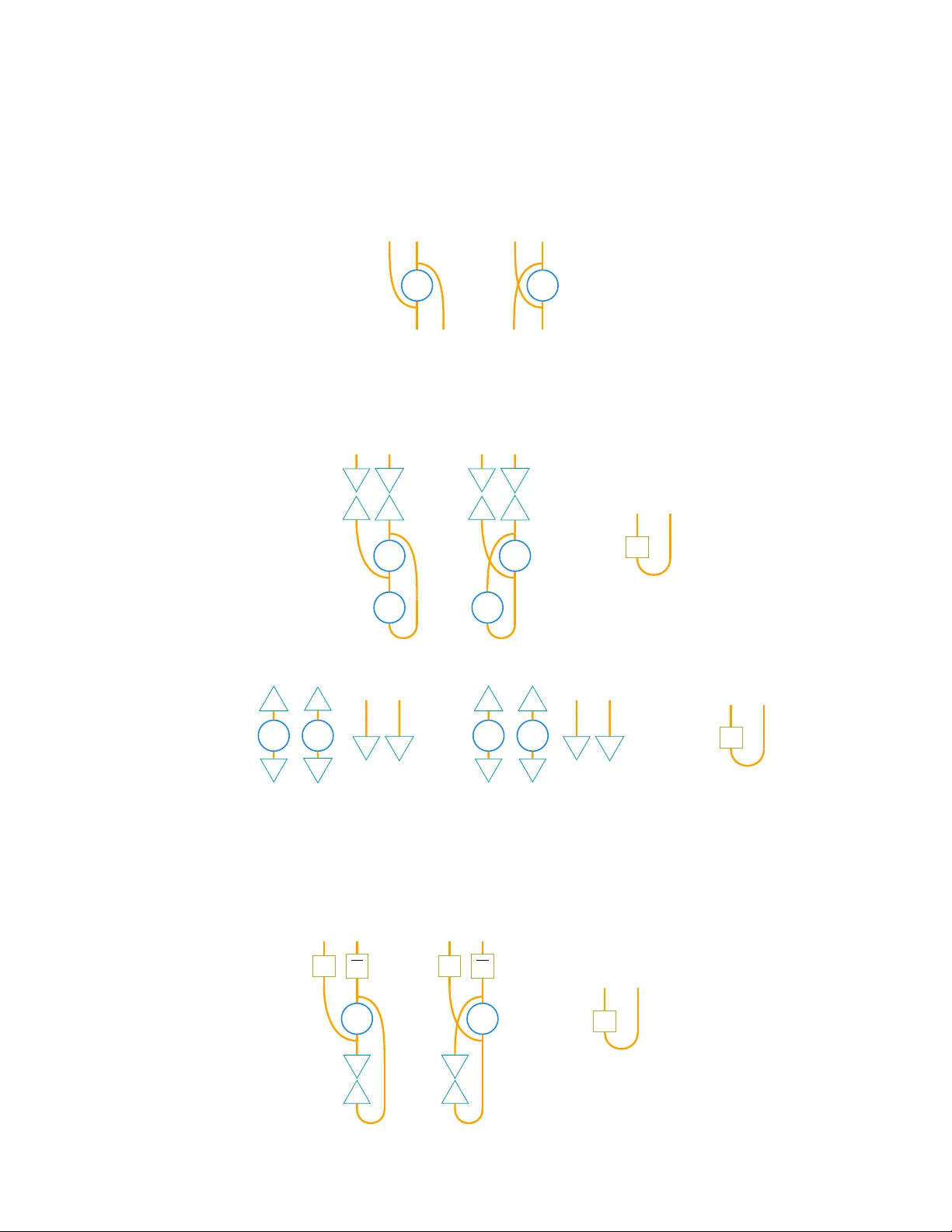
Quan tum Graph Theory b y Example Gian Luca Spitzer ∗ 1,2 and Ion Nec hita † 2 1 L aBRI, Université de Bor de aux, CNRS, Bor de aux INP, UMR-5800, F r anc e 2 L ab or atoir e de Physique Thé orique, Université de T oulouse, CNRS, UPS, F r anc e Abstract Quan tum graphs ha ve b een introduced by Duan, Severini, and Winter to describ e the zero-error b eha viour of quan tum c hannels. Since then, quan tum graph theory has become a ﬁeld of study in its o wn righ t. A substan tial source of diﬃculty in w orking with quan tum graphs compared to classical graphs stems from the fact that they are no longer discrete objects. This makes it generally diﬃcult to construct insigh tful, non-trivial examples. W e presen t a collection of non-trivial quantum graphs that can b e thought of in discrete terms, and that can be expressed in the diagrammatic formalism introduced by Musto, Reutter, and V erdon. The examples arise as the quantum graphs acted on b y increasingly smaller classical matrix groups, and are parametrised b y triples of matrices ( A, B , C ) . The parametrisation rev eals a clean decomp osition of quantum graph structure in to classical and genuinely quantum comp onents: A and C are describ ed b y a classical w eighted graph called the strange graph, while B pro vides a purely quan tum con tribution with no classical analogue. Based on this mo del, we give exact formulas or establish b ounds for quantum graph parameters, such as the num b er of connected components, the c hromatic n umber, the indep endence num b er, and the clique n umber. Our results pro vide the ﬁrst large, parametric families of quan tum graphs for whic h standard graph parameters can b e computed analytically . Con ten ts 1 In tro duction 2 2 Preliminaries 4 2.1 Quan tum Sets and String Diagrams . . . . . . . . . . . . . . . . . . . . . . . . . . . . . . . . 4 2.2 Quan tum Graphs . . . . . . . . . . . . . . . . . . . . . . . . . . . . . . . . . . . . . . . . . . . 7 2.3 Prop erties of Quantum Graphs . . . . . . . . . . . . . . . . . . . . . . . . . . . . . . . . . . . 10 3 Classical Matrix Groups A cting on Quan tum Graphs 13 3.1 The Unitary and the Orthogonal Group . . . . . . . . . . . . . . . . . . . . . . . . . . . . . . 13 3.2 The Diagonal Unitary and the Diagonal Orthogonal Group . . . . . . . . . . . . . . . . . . . 16 3.3 The Hyp ero ctahedral Group . . . . . . . . . . . . . . . . . . . . . . . . . . . . . . . . . . . . . 20 3.4 Classical Mo dels of Quantum Graphs . . . . . . . . . . . . . . . . . . . . . . . . . . . . . . . . 22 4 Graph Theoretic Prop erties 24 4.1 Connected Comp onen ts . . . . . . . . . . . . . . . . . . . . . . . . . . . . . . . . . . . . . . . 24 4.2 Colouring . . . . . . . . . . . . . . . . . . . . . . . . . . . . . . . . . . . . . . . . . . . . . . . 34 4.3 Indep enden t Sets . . . . . . . . . . . . . . . . . . . . . . . . . . . . . . . . . . . . . . . . . . . 40 4.4 Cliques . . . . . . . . . . . . . . . . . . . . . . . . . . . . . . . . . . . . . . . . . . . . . . . . 46 5 Conclusion 56 ∗ gian-luca.spitzer@u-bordeaux.fr † nechita@irsamc.ups-tlse.fr 1 1 In tro duction Graph theory is one of the most v ersatile branches of discrete mathematics, with applications ranging from computer science and combinatorial optimisation to statistical physics and netw ork science. Many of its cen tral notions such as colouring, connectivity , indep endence, cliques, etc. ha ve been studied for ov er t wo cen turies [ Die25 ]. A natural question, motiv ated by the adven t of quan tum information theory , is whether these notions admit meaningful generalisations to a non-comm utative setting, where the vertex set of a graph is replaced b y a quantum set and the adjacency relation b y a suitable op erator-algebraic structure. The origins of quantum gr aph the ory can b e traced to the work of W eav er [ W ea10 ] who introduced quan tum graphs as sp ecial cases of quantum r elations , and the work of Duan, Sev erini, and Winter [ DSW13 ], who in tro duced the c onfusability gr aph of a quantum channel as a non-comm utative generalisation of Shannon’s classical confusabilit y graph [ Sha56 ]. The former approach in tro duces a notion of relations on v on Neumann algebras, deﬁning a quantum graph as a reﬂexive, symmetric quantum relation. The latter approach considers op erator spaces of the form span { K ∗ i K j | i, j ∈ [ m ] } , where K 1 , . . . , K m are the Kraus op erators of a quantum c hannel. Suc h an op erator space encodes the c hannel’s confusability structure and pla ys the role of the edge set of a graph. This p ersp ective opened the do or to extending classical zero-error information theory to the quan tum setting [ Sta15 ], and led to the discov ery of striking phenomena suc h as superactiv ation of zero-error capacit y [ Dua09 , CCH11 ]. A systematic mathematical framework for quan tum graphs w as subsequently dev elop ed from tw o comple- men tary p ersp ectives. On the op erator-algebraic side, W ea ver [ W ea21 ] expanded on the theory of quantum relations on v on Neumann algebras. This approac h, ro oted in op erator space theory , naturally extends classical notions of indep endent sets and cliques [ W ea17 ] and has led to quan tum analogues of Ramsey’s theorem. On the categorical side, Musto, Reutter, and V erdon [ MR V18 ] prop osed a comp ositional approach in whic h a quan tum graph is deﬁned as an adjac ency op er ator on a quan tum set, the latter b eing formalised as a sp ecial symmetric † -F robenius monoid in the category of ﬁnite-dimensional Hilb ert spaces. This form ulation comes equipp ed with a pow erful string diagr ammatic c alculus [ HV19 , Vic11 ] that makes man y pro ofs visual and in tuitive. In the ﬁnite-dimensional case, which is the setting of this pap er, b oth approac hes are equiv alent. These foundational w orks hav e initiated a rapidly gro wing b o dy of research; w e refer the reader to the surv ey by Da ws [ Daw24 ] for a comprehensive account of the diﬀerent persp ectives on quan tum graphs and their interrelations. Graph-theoretic prop erties hav e b een generalised to the quantum setting: colouring and c hromatic num b ers via non-lo cal games [ BGH22 , Gan23 ], capacit y b ounds and Lov ász-type parameters via sandwic h theorems [ BTW21 ], connectedness and algebraic connectivity via sp ectral and op erator-algebraic metho ds [ CGW25 , Mat24 ], and graph homomorphisms and isomorphisms via categorical and game-theoretic framew orks [ Ats+19 , Bra+20 , Gol26 ]. Classical graph constructions hav e also b een p orted to the quantum setting, including the Mycielski transformation [ BK25 ]. At the same time, the question of classifying quan tum graphs and constructing explicit examples has receiv ed increasing attention. Gromada [ Gro22 ] classiﬁed all quan tum graphs on M 2 , ﬁnding exactly four non-isomorphic simple quantum graphs, and further constructed examples from Hadamard matrices [ Gro24 ]; see also the related w ork of Matsuda [ Mat22 ]. Despite this progress, the theory has un til no w lac ked a supply of concrete, parametric families of quantum graphs for whic h graph-theoretic parameters can b e computed analytically . Classical graph theory b eneﬁts enormously from explicit families (circulant graphs, Kneser graphs, P aley graphs, etc.) that serve as examples, coun terexamples, and testing grounds for conjectures. Recent work of W asilewski [ W as24 ] on quantum Cayley graphs is a step in this direction. The present paper aims to ﬁll this gap more broadly for quantum graphs. The contributions of this work are tw ofold: W e introduce and then thoroughly study new families of quan tum graphs on M n that are in v ariant under the action of some classical matrix groups. On the conceptual side, we introduce and study families of quantum graphs on M n that are inv ariant under the action of classical matrix groups, suc h as the unitary group, the orthogonal group, and their resp ectiv e diagonal subgroups. The guiding principle is the same as in classical graph theory: Just as considering smaller subgroups of the symmetric group S n yields larger and richer families of classical graphs, considering smaller subgroups of the unitary group U ( n ) yields larger families of quantum graphs. Apart from the unitary group itself, we lo ok 2 at the orthogonal group O ( n ) and the h yp ero ctahedral group Hyp ( n ) , as w ell as the diagonal fragmen ts of U ( n ) and O ( n ) : the diagonal unitary gr oup D U ( n ) and the diagonal ortho gonal gr oup D O ( n ) . These satisfy the follo wing inclusions. U ( n ) ⊇ O ( n ) ⊇ Hyp( n ) ⊇ D O ( n ) ⊆ D U ( n ) . Requiring in v ariance under the full unitary group U ( n ) yields only the complete quantum graph K n and the edgeless quan tum graph K c n , while the orthogonal group O ( n ) additionally permits the symmetric and antisymmetric quantum gr aphs G sym and G asym (Prop osition 3.13 ). These are already genuinely quantum ob jects with no classical counterpart. The diagonal unitary group D U ( n ) and the diagonal orthogonal group D O ( n ) are considerably smaller, and their inv ariant quan tum graphs form the main ob ject of study of this pap er. Building on the characterisation of D U ( n ) - and D O ( n ) -in v ariant linear maps [ SN21 , NS21 ], we show that these quantum graphs are parametrised b y three n × n matrices A , B , C with matc hing diagonals, giving rise to quan tum graphs denoted X A,B ,C (Prop osition 3.10 ). The conditions for X A,B ,C to b e a quantum graph decomp ose cleanly: B m ust b e a pro jector, and for all i  = j the 2 × 2 blo cks  A ij C ij C j i A j i  m ust b e pro jectors. Each of the three matrices pla ys a very distinct role: • The matrix A enco des a classic al gr aph on n v ertices. When B and C are trivial, the quan tum graph X A, diag A is precisely the em b edding of a classical graph in to M n (Corollary 3.12 ). • The matrix C in tro duces a new type of edges, whic h w e call str ange e dges , annotated with a phase θ ∈ [0 , 2 π ) . T ogether, A and C determine a classical mo del called the str ange gr aph G ( A, C ) , which can b e though t of as a classical graph whose edges are either classical or strange (see Section 3.4 ). • The matrix B is a pur ely quantum c ontribution : a pro jector on C n with no classical analogue, which can b e thought of as attaching a subspace to the quan tum graph. This decomp osition captures an increasing level of “quan tumness” as one mov es from purely classical graphs X A, diag A through AB graphs X A,B (whic h are D U ( n ) -in v ariant) to full ABC graphs X A,B ,C ha ving D O ( n ) symmetry . Our second main con tribution is the computation of graph-theoretic parameters for these newly in tro duced quan tum graphs. On the concrete side, we compute graph-theoretic parameters for the newly in tro duced families of quan tum graphs, such as connectedness, colouring, independent sets, and cliques. A k ey structural observ ation underlying our results is a recurring splitting principle : F or each of the graph parameters w e consider, the deﬁning conditions decomp ose in to indep endent conditions on the ( A, C ) part and the B part (Prop osition 4.5 and analogues for colouring, indep endent sets, and cliques). This eﬀectively reduces problems about quantum graphs to a com bination of a classical graph problem determined by the strange graph G ( A, C ) , and a linear-algebraic problem inv olving the pro jector B . W e highlight ﬁv e of our most imp ortan t results: 1. Connectedness. F or n ≥ 3 , a quantum graph X A,B ,C is connected if and only if its strange graph G ( A, C ) is connected (Prop osition 4.15 ). This equiv alence can fail for n = 2 : Isolated strange edges with phase π giv e rise to quan tum graphs with strictly more connected components than their strange graph (Prop osition 4.13 ). 2. Indep endence n umber. The indep endence num b er of quantum graphs of the form X A, diag A,C is completely determined b y the strange graph: α ( X A, diag A,C ) = α ( G ( A, C )) (Prop osition 4.27 ). F or the purely quantum part, the independence num ber of X diag B,B can b e b ounded in b oth directions in terms of the rank of B . It is also lo wer bounded b y EqRo ws ( B ) , the maximum num b er of equal ro ws of B in the standard basis. 3 3. Non-colourabilit y . There exist quan tum graphs that are not classically colourable at all (Prop osi- tion 4.18 ); this includes the complete quantum graph K n and the symmetric quantum graph G sym for n ≥ 3 . In contrast, quantum graphs of the form X diag B,B are alw ays n -colourable (Proposition 4.19 ), sho wing that the obstruction to colourability arises from the in teraction b etw een A , C , and B . 4. Clique n umber. The quantum clique num b er of the quantum graph induced b y a classical graph ω ( X A, diag A ) can diﬀer dramatically from the classical clique num b er ω ( A ) , in both directions. While ω ( X A, diag A ) ≥ ω ( A ) − 1 alw ays holds, the classical complete bipartite graph on n v ertices satisﬁes ω ( A ) = 2 but ω ( X A, diag A ) ≥ n/ 2 (Prop osition 4.43 ). On the other hand, the classical complete graph satisﬁes ω ( X A, diag A ) = n − 1 < n = ω ( A ) (Proposition 4.44 ). The symmetric and antisymmetric quan tum graphs b oth ha ve clique n umber ⌈ n/ 2 ⌉ . 5. The role of B . The matrix B con tributes a form of quan tum density that in teracts non-trivially with the classical structure enco ded b y A and C . F or example, ω ( X diag B,B ) ≤ √ rk B + 1 (Prop osition 4.39 ), while X diag B,B alw ays has n connected components and is n -colourable. Most of the results presented in this pap er are summarized in T able 1 , whic h classiﬁes quan tum graphs according to their underlying classical symmetry and gathers all the exact formulas and b ounds for their graph prop erties. The paper is organized as follows. Section 2 introduces the necessary bac kground on quan tum sets, quan tum graphs, and their diagrammatic calculus, as w ell as the classical matrix groups and graph-theoretic prop erties studied throughout the paper. Section 3 develops the theory of quantum graphs inv ariant under classical matrix groups, culminating in the parametrisation of D U ( n ) - and D O ( n ) -in v ariant quan tum graphs b y triples of matrices ( A, B , C ) . Section 4 computes graph-theoretic parameters for the families of quan tum graphs in tro duced in the previous section: connected comp onents, c hromatic num b er, indep endence num b er, and clique n umber. Finally , Section 5 summarises our ﬁndings and discusses open problems. 2 Preliminaries First, let us ﬁx some general conv en tions. W e assume all pro jectors to b e orthogonal projectors: A linear map P on a Hilbert space is a pro jector if P 2 = P † = P . W e use I to denote diﬀeren t identities. It ma y refer to the identit y linear map on some arbitrary v ector space, or explicitly to the identit y matrix in M n . It will alw ays b e clear from the context whic h is mean t. When talking ab out classical graphs, w e assume the vertex set to b e [ n ] := { 1 , . . . , n } . W e write i ∼ j if the vertices i and j are adjacent. 2.1 Quan tum Sets and String Diagrams W e will view quantum graphs as adjacency operators on a quantum set of v ertices. As can b e motiv ated through Gelfand dualit y of sets (viewed as ﬁnite spaces with the discrete topology), a quantum set is a ﬁnite-dimensional C ∗ -algebra. It is known [ Vic11 , Theorem 4.7] that the category of C ∗ -algebras is equal to the category of sp e cial symmetric † -F r ob enius monoids in fdHilb . Deﬁnition 2.1. A monoid X in fdHilb is a ﬁnite-dimensional Hilb ert space equipp ed with a linear map m : X ⊗ X → X , called multiplic ation , and a linear map u : C → X , called unit , satisfying 1. m ◦ (id ⊗ m ) = m ◦ ( m ⊗ id) (asso ciativit y), 2. m ◦ (id ⊗ u ) = m ◦ ( u ⊗ id) = id (unitality). No w the category fdHilb is canonically equipped with a contra v ariant endofunctor † that is the iden tity on ob jects, and maps a linear map f : X → Y b et ween Hilb ert spaces X, Y to its adjoint f † : Y → X . In particular, a monoid in fdHilb is automatically equipp ed with a c omultiplic ation m † : X → X ⊗ X and a c ounit u † : X → C . They satisfy the adjoints of conditions (1) and (2), called coasso ciativit y and counitalit y . Deﬁnition 2.2. A † -F r ob enius monoid X is a monoid satisfying the F r ob enius pr op erty , 4 1. (id ⊗ m ) ◦ ( m † ⊗ id) = m † ◦ m = ( m ⊗ id) ◦ (id ⊗ m † ) . It is called 2. sp e cial if m ◦ m † = id , 3. symmetric if σ ◦ m † ◦ u = m † ◦ u , where σ is the swap map. The adv an tage of working in a monoidal category like fdHilb is that we get access to a p ow erful graphical calculus that allo ws us to reason formally b y manipulating string diagr ams . This approach of working with quan tum sets and quantum graph w as ﬁrst in tro duced by Musto, Reutter, and V erdon in [ MR V18 ], where w e also refer the reader for a more detailed introduction. F urther exp osition of the theory of string diagrams and their applications can be found in [ HV19 , Vic11 ]. The primitiv es of the calculus are strings (or wir es ) and b oxes . f Strings represen t ob jects, while b oxes represent morphisms. In our case the strings represen t (elements of ) Hilb ert spaces, while b oxes are linear maps. Comp osition g ◦ f of functions is represented by serial comp osition of diagrams, while tensor pro ducts f ⊗ h are represen ted by parallel comp osition. Diagrams are read from b ottom to top. f g f h The monoidal unit, C in the case of fdHilb , is represen ted by the empty diagram. Linear maps C → X are th us represented b y a b ox that only has an outgoing wire. F or reasons that will become apparent later, we generally represen t such maps b y a triangle with a corner cut oﬀ. x (1) The m ultiplication and unit maps of monoids are represented as fusion of wires and dots resp ectiv ely . T aking adjoin ts in the diagrammatic calculus corresp onds to mirroring the diagram across a horizon tal axis. As suc h, the comultiplication and counit are represen ted as follows. The F robenius prop ert y , for instance, can thus be expressed graphically as = = . A ﬁnal imp ortant class of maps are the cups and caps. : = : = 5 These are the duality morphisms for X , and their deﬁnition in terms of (co)m ultiplication and (co)unit sho ws that † -F robenius monoids are self-dual. 1 F or our purp oses, it suﬃces to know that they allow us to deﬁne the transp ose of a linear map. Deﬁnition 2.3. Let f : X → Y b e a linear map b etw een tw o † -F robenius monoids. Its tr ansp ose is the map f T : Y → X deﬁned as f T = f . (2) The pow er of string diagrams is that they can b e used in lieu of symbolic equations to pro ve equalities. Concretely , ev ery equation that can b e derived in the diagrammatic calculus b y moving and b ending strings, sliding b o xes along wires, and rotating boxes also holds in fdHilb . This can b e stated formally . Theorem 2.4 (Theorem 3.28 in [ HV19 ]) . In a pivotal c ate gory, a wel l-forme d e quation b etwe en morphisms fol lows fr om the axioms if and only if it holds in the gr aphic al c alculus up to planar oriente d isotopy. A pivotal category is a category with duals in whic h ev ery object is naturally isomorphic to its double dual. Clearly , fdHilb is a pivotal category , so the theorem applies. Theorems of this form are often called c oher enc e the or ems , and they also exist for other t yp es of categories, cf. [ Sel11 ]. One suc h planar oriented isotopy w ould b e to consider the righ t-hand side of Equation ( 2 ) and pulling the bent wires taut. This will result in a 180 degree rotation of the f b o x. W e conclude that taking the transp ose of a linear map corresponds to rotating the corresp onding diagram b y 180 degrees. By using non-symmetric boxes for maps, w e may thus get rid of sup erscripts to represent transp oses and adjoints. W e let f f = , f f T = , f f † = , f f = . The last equation corresp onds to the conjugate of a linear map, deﬁned as f = ( f † ) T = ( f T ) † . The corresp onding op eration in the diagrammatic calculus m ust thus b e mirroring across a horizontal axis, follow ed b y a 180 degree rotation (or vice versa). This corresp onds to mirroring across a v ertical axis. Despite being useful, this asymmetric notation has the tendency to introduce visual clutter. Since we will rarely need adjoints or transp oses of maps X → X , we reserve this asymmetric notation for maps C → X , see Equation ( 1 ). Example 2.5 (Classical Sets) . By Gelfand duality , the classical set with n elemen ts corresp onds to the quan tum set C n . This b ecomes a sp ecial symmetric † -F rob enius monoid as follows. W e c ho ose an orthonormal basis | 1 ⟩ , . . . , | n ⟩ , the standar d b asis , and deﬁne m as the linear extension of C n ⊗ C n → C n , | i ⟩ ⊗ | j ⟩ 7→ δ ij | i ⟩ . In other words, the m ultiplication on C n is comp onent wise. The unit with resp ect to this m ultiplication m ust then b e given by C → C n , c 7→ c 1 , where 1 : = n X k =1 | k ⟩ . F rom this, the comultiplication can be determined to b e the linear extension of C n → C n ⊗ C n , | i ⟩ 7→ | i ⟩ ⊗ | i ⟩ , while the counit is the sum-of-en tries map C n → C . Note that the comultiplication only copies elemen ts of the standard basis; this is the no-cloning the or em . Equiv alently , we could ha ve started with the com ultiplication 1 Otherwise, we would hav e to annotate our strings with arrows, as is done in [ Vic11 ]. 6 and deﬁned the standard basis as precisely the elements that are copied by the comultiplication, cf. [ CPV13 , Theorem 5.1]. It is not hard to verify using the ab ov e deﬁnitions that standard basis elemen ts must b e self-conjugate, | i ⟩ = ( | i ⟩ † ) T = | i ⟩ . Recalling that taking the conjugate of a linear map corresp onds to mirroring the diagram across a vertical axis, w e w ant the b oxes represen ting self-conjugate maps to hav e this symmetry . W e thus represen t standard basis elements as full triangles, as opposed to the cut triangles of Equation ( 1 ). i Finally , given some linear map f : C n → C n , one ma y verify that the transpose as deﬁned in Deﬁnition 2.3 is precisely giv en by the transpose of the matrix representation of f in the standard basis. ⌟ In this pap er, we will mainly b e interested in one particular family of quantum sets, the ful l matrix algebr as M n ( C ) for n ≥ 2 . These are obviously ob jects of fdHilb and they form a † -F rob enius monoid by setting u ( c ) = cI , m ( X ⊗ Y ) = X Y . They also admit a reﬁnemen t of the string diagrammatic formalism. Namely , there is an isomorphism M n ∼ = C n ⊗ C n . This means that instead of representing M n as a single wire, we ma y represent it as t wo parallel C n wires. The isomorphism is then given graphically as M n → C n ⊗ C n , x 7→ x . This is sometimes called the “vectorisation map” and corresp onds to stacking the columns of x on top of eac h other. The multiplication and unit maps are then giv en by = , = . Concretely , this is the endomorphism monoid of C n , cf. [ Vic11 , Deﬁnition 3.16]. Endomorphism monoids alw ays satisfy the F rob enius prop erty , and it is a go o d exercise to verify that M n is symmetric since C n is. Ho wev er, deﬁned this wa y M n is not sp ecial. W e hav e = = n = n  = . This is closely related to so called δ -forms, cf. e.g. [ Gro22 , Section 1]. W e can make M n sp ecial by normalising u, u † , m, m † . In fact, there are m ultiple wa ys to accomplish this. The normalisation most common in the con text of string diagrams is ˜ m = 1 √ n m, ˜ u = √ nu, ˜ m † = 1 √ n m † , ˜ u † = √ nu † . This normalisation preserv es the prop erty that taking the adjoint corresp onds to simply mirroring the diagram. In what follows, w e will generally suppress these normalisation factors. This is b ecause the normalisation will lead to factors in unexp ected places, at the cost of readability . Since we will mostly b e w orking in the diagrammatic calculus, this will hav e almost no impact on our arguments. W e only need to remember the normalisation when w e wan t to compute scalars. 2.2 Quan tum Graphs There are man y diﬀerent equiv alent w ays of deﬁning quan tum graphs. W e will b e interested in t wo of them. Firstly , a quantum graph is an adjacency operator on a quantum set of v ertices. 7 Deﬁnition 2.6 (cf. Deﬁnition V.1 in [ MR V18 ]) . A quantum gr aph is a tuple ( X, G ) , where X is a quantum set and G : X → X is a linear map satisfying G G = G and G = G † The tw o prop erties abstract the deﬁning prop erties of adjacency matrices. In the classical case, where wires are C n , the ﬁrst condition says that G is idemp otent under the en trywise (Sch ur) pro duct. The second condition says that G is self-conjugate, or in the classical case that its matrix representation in the standard basis has real en tries. 2 When the quan tum set X is clear from the con text, we will also identify a quantum graph G with its adjacency op erator. Deﬁnition 2.7. A quantum graph ( X , G ) 1. is undir e cte d if = G G 2. has no lo ops if G = 0 3. has lo ops at every vertex if G = . Remark 2.8. Recall that we will generally suppress the normalisation of multiplication and comultiplication that mak es the † -F rob enius monoid M n sp ecial. This will hav e an impact on what constitutes an adjacency op erator of a quan tum graph. How ever, it is straightforw ard to reco ver the adjacency op erators for sp ecial † -F rob enius monoids: W e simply multiply the adjacency op erator b y n . Indeed, let A b e a v alid adjacency op erator in the non-normalised setting, that is m ◦ ( A ⊗ A ) ◦ m † = A. Let A ′ = nA . The realness condition is inv arian t under multiplication by real scalars. Moreo ver, p er deﬁnition w e get ˜ m ◦ ( A ′ ⊗ A ′ ) ◦ ˜ m † = 1 n m ◦ ( nA ⊗ nA ) ◦ m † = nA = A ′ , so A ′ is an adjacency operator in the normalised setting. The same reasoning applies to the undirectedness and lo op conditions. 2 Note that in the classical case, the second prop erty is redundan t, since b eing idempotent under the Hadamard pro duct already requires the matrix entries in the standard basis to b e in the set { 0 , 1 } . How ever, adding the realness condition leads to a more coherent theory . 8 The second imp ortant characterisation of quan tum graphs will b e in terms of op erator spaces. F rom now on w e will only consider quan tum graphs on M n . The isomorphism M n ∼ = C n ⊗ C n allo ws us to deﬁne the r e alignment map, ( − ) R : End( M n ) → End( M n ) , F 7→ F , whic h sw aps the bottom-right and top-left tensor legs of a linear map M n → M n . In the quantum information literature, the realignment map is used for en tanglement detection [ R ud00 , Rud03 ], and the resulting map is called the Choi matrix [ Cho75 ]; see also [ BZ06 , Section 10.2]. It is easy to see that the realignment is an in volution, that is, ( F R ) R = F . W e can thus give an equiv alent deﬁnition of quantum graphs b y taking the realignmen t of the conditions in Deﬁnition 2.6 . Prop osition 2.9. A line ar map G is the adjac ency op er ator of a quantum gr aph if and only if G R is a pr oje ctor. Pr o of. T aking the realignment of the Sch ur idemp otency condition and writing it in terms of G R yields G R = G R G R = G R G R , where the second equalit y follows from isomorphism of diagrams. The realness condition b ecomes ( G R ) † G † G = G † = = G R = . These are precisely the conditions ( G R ) 2 = G R and ( G R ) † = G R . ■ Ev ery pro jector on M n uniquely deﬁnes a subspace S ⊆ M n , so quantum graphs can equiv alently b e viewed as op er ator sp ac es [ Pau02 ]. This is a p ersp ective that is often taken in the op erator algebra- and the quantum information literature. The latter is b ecause one can naturally asso ciate to a quantum c hannel Φ with Kraus op erators K 1 , . . . , K m the op erator space span { K † i K j | i, j ∈ [ m ] } , called the quantum c onfusability gr aph of Φ . This generalises classical confusability graphs [ Sha56 ], extending the theory of Shannon capacities to the quan tum case [ DSW13 ]. Analogous to the pro of of Proposition 2.9 one may translate the conditions for undirectedness and having (no) lo ops into the op erator space picture. This yields the follo wing characterisation, see also [ W ea21 ]. Prop osition 2.10. L et G b e a quantum gr aph and S = img G R the op er ator sp ac e asso ciate d to it. Then 1. G is undir e cte d if and only if X ∈ S ⇒ X † ∈ S , 2. G has lo ops at every vertex if and only if I ∈ S . 9 3. G has no lo ops if and only if X ∈ S ⇒ T r( X ) = 0 . As is usual in classical graph theory , we will restrict our attention to simple quan tum graphs, that is undirected quantum graphs without loops. Note that in the literature, many authors instead w ork in a setting where quantum graphs hav e lo ops at every vertex. This setting is more natural in the context of confusabilit y graphs, cf. [ DSW13 ]. How ever, just as for classical graphs, there is a natural corresp ondence b et ween lo opless quantum graphs and quan tum graphs with lo ops at every v ertex, which is a direct corollary of Prop osition 2.10 . Prop osition 2.11. L et S b e the op er ator sp ac e of a lo opless quantum gr aph. Then S ⊕ C I is the op er ator sp ac e of a quantum gr aph with lo ops at every vertex. Conversely, for every op er ator sp ac e S ′ of a quantum gr aph with lo ops at every vertex, S ′ ⊖ C I is the op er ator sp ac e of a lo opless quantum gr aph. This is equiv alent to the following statement ab out adjacency operators, which directly generalises the classical case. Prop osition 2.12. L et G b e a lo opless quantum gr aph. Then G + I is a quantum gr aph with lo ops at every vertex. Conversely, for a quantum gr aph H with lo ops at every vertex, H − I is a lo opless quantum gr aph. Pr o of. By Proposition 2.10 , G R pro jects on to a subspace orthogonal to C I . This means that G R + ΩΩ † is a projector, where ΩΩ † is the rank- 1 pro jector on to the identit y matrix I ∈ M n . Letting S = img G R , this pro jects precisely onto S ⊕ C I . A t the same time, the realignment of the iden tity on M n is giv en by = , whic h is precisely ΩΩ † . It follo ws that ( G + I ) R = G R + ΩΩ † as desired. Similarly , H R pro jects onto a subspace S ′ with I ∈ S ′ . This implies that ( H − I ) R = H R − ΩΩ † is a pro jector with image S ′ ⊖ C I . ■ 2.3 Prop erties of Quantum Graphs Most fundamen tal deﬁnitions of classical graph theory hav e been generalised to the quan tum case. In this pap er, w e fo cus on four concepts: connected comp onents, colouring, independent sets, and cliques. Connected Comp onen ts. Let G b e a quantum graph. Courtney , Ganesan, and W asilewski [ CGW25 ] deﬁne G to b e c onne cte d if L p G = GL p = ⇒ p ∈ { 0 , I } for all projectors p ∈ M n , where L p denotes left m ultiplication by p . Note that this is equiv alent to saying that G is disc onne cte d if there exists a non-trivial pro jector p such that L p GL p ⊥ = 0 , where p ⊥ is the pro jector onto ker p . Left multiplication can be expressed graphically in a simple wa y: x x x = = W e can thus restate the deﬁnition of connectedness nicely in graphical terms. 10 Deﬁnition 2.13. A quantum graph G is disc onne cte d if there exists a non-trivial pro jector P : C n → C n suc h that G P = 0 P ⊥ . (3) Otherwise G is called c onne cte d . As men tioned in [ CGW25 ], L p should be thought of as the pro jector onto a connected comp onent of G . This immediately suggests the follo wing deﬁnition for connected comp onen ts. Deﬁnition 2.14. A quantum graph G has (at least) k c onne cte d c omp onents if there exist projectors P 1 , . . . , P k on C n with P s P s = I such that G P s = 0 P t for all s  = t . Observ e that for k = 1 the condition is satisﬁed v acuously , so a connected graph still has at least 1 connected component. Con versely , if G is disconnected then there exists a projector P satisfying Equation ( 3 ). In this case the c hoice P 1 = P , P 2 = P ⊥ witnesses that G has at least t wo connected components. Colouring. A deﬁnition of graph colouring for quan tum graphs w as in tro duced b y Brannan, Ganesan, and Harris [ BGH22 ] in the con text of non-lo cal games. As common in the non-lo cal games literature, they actually in tro duce m ultiple v ersions of colouring that diﬀer in strength based on how correlated the answ ers of play ers in a certain non-local game are allo wed to b e. W e will only consider classic al colourings, whic h corresp ond to classical winning strategies in the colouring game. T ranslated into our language, the deﬁnition reads as follo ws. Deﬁnition 2.15 (cf. Deﬁnition 2.15 in [ Gan23 ]) . Let G b e a quantum graph and S = img G R its asso ciated op erator space. Then G has a k -c olouring if there exist pro jections P 1 , . . . , P k with P s P s = I such that P s X P s = 0 for all X ∈ S and s ∈ [ k ] . W e can express this condition graphically as G R x P s P s = 0 , 11 whic h has to hold for all x ∈ M n and s ∈ [ k ] . W e can get rid of the x and write the condition in terms of the adjacency op erator, which yields = 0 G P s P s ⇐ ⇒ = 0 G P s P s . Finally , we can take the conjugate of b oth sides, which reco vers an equiv alent condition analogous to the one for connected comp onents. Deﬁnition 2.15’. A quantum graph G has a k -c olouring if there exist pro jectors P 1 , . . . , P k on C n with P s P s = I such that G P s = 0 P s for all s ∈ [ k ] . The chr omatic numb er χ ( G ) of a quantum graph G is deﬁned as the smallest k suc h that G has a k -colouring. Indep enden t Sets. There are multiple p ossible generalisations of indep endent sets to quantum graphs—cf. [ DSW13 , Proposition 2]—that are more or less natural dep ending on whether one approac hes the problem from the p ersp ective of classical graph theory , or op erationally from the p ersp ective of quantum channels and their confusabilit y graphs. In this paper, we will deﬁne an independent set as follo ws. Deﬁnition 2.16 (cf. Deﬁnition 1.1 in [ W ea17 ]) . Let S ⊆ M n b e the op erator space corresp onding to a quan tum graph G . A k -indep endent set of G is a pro jector P ∈ M n of rank k suc h that P S P ⊆ C P . The indep endenc e numb er α ( G ) is the largest k such that G has a k -indep endent set. Note that our deﬁnition slightly diﬀers from that given by W eav er in [ W ea17 ] and Duan, Severini, and Win ter in [ DSW13 ]. There they require that P S P = C P , whic h is precisely the Knill-Laﬂamme error correction condition [ KL97 ]. This means that if S represen ts the confusability graph of a quan tum channel, then an indep endent set is precisely a co de that allo ws for zero-error communication. The reason wh y we mo dify this deﬁnition is that for confusability graphs, S is an op erator system , that is it is closed under adjoin ts and, crucially , contains the iden tity . This means that P S P alw ays con tains at least P I P = P , and th us C P ⊆ P S P . W e work in a more general framework, where quantum graphs are arbitrary op erator spaces. Since w e w ant to w ork with lo opless quantum graphs, our deﬁnition needs to account for the possibility that there is no X ∈ S suc h that P X P = P . This yields the condition P S P ⊆ C P . Graphically , we can express Deﬁnition 2.16 as follo ws, where G R is the pro jector on to the operator space and c x ∈ C is a (p otentially zero) scalar. G R x P P = c x · P ⇐ ⇒ G R x P P = c x · P The condition has to hold for all x ∈ M n . 12 Cliques. T o deﬁne cliques, w e again stic k to the deﬁnition giv en in [ W ea17 ]. While other natural deﬁnitions exist, this one has been studied in-depth and for example permits a generalisation of Ramsey’s theorem to quan tum graphs, as prov ed in the ab ov e-men tioned pap er. Just as for indep endent sets, w e adapt W eav er’s deﬁnition to accoun t for quantum graphs without loops. Deﬁnition 2.17 (cf. Deﬁnition 1.1 in [ W ea17 ]) . Let S ⊆ M n b e the op erator space corresp onding to a quan tum graph G . A k -clique of G is a projector P ∈ M n of rank k , suc h that P ( S ⊕ C I ) P = P M n P . The clique numb er ω ( G ) is the largest k such that G has a k -clique. 3 Classical Matrix Groups A cting on Quan tum Graphs T o construct our examples of quantum graphs, w e turn our attention to group actions. Classically , subgroups of the symmetric group S n act on a classical graph by p ermuting its v ertices. Concretely , given such a subgroup X ⊆ S n , realised as n × n p erm utation matrices, and a classical graph G with adjacency matrix A ∈ { 0 , 1 } n × n , we say that X acts on G if P A = AP for all P ∈ X . No w it is easy to see that if X = S n , the only loopless graphs that X acts on are the complete graph A = J − I and the empt y graph A = 0 . As one considers smaller and smaller X ⊆ S n , one obtains larger and larger classes of graphs. The cyclic group Z n ⊆ S n , for instance, yields precisely the circulan t graphs. W e apply this reasoning to quan tum graphs on M n , where the unitary group U ( n ) tak es the role of S n . Natural choices of subgroups X ⊆ U ( n ) will yield diﬀeren t classes of quantum graphs, whic h hav e in common that they can b e though t of in discrete terms and are amenable to study in the diagrammatic calculus. W e b egin by establishing what it means for a classical matrix group to act on a quantum graph. Recall that just as in the classical case, a quan tum graph is a (quan tum) set of v ertices together with some extra structure. In particular, a group acting on a quantum graph should ﬁrst and foremost act on the set of vertices. Note that w e hav e M n ∼ = End ( C n ) . This means that there is already a v ery natural action of subgroups of GL ( C n ) ⊆ End ( C n ) —conjugation. How ever, since we view M n as a C ∗ -algebra, w e require the group action to preserve the C ∗ -in volution. In the case of M n this is the Hermitian adjoint, so we must restrict to the unitary group. Observ ation 3.1. A sub gr oup of U ( n ) acts on M n by c onjugation, that is, α : U ( n ) × M n → M n deﬁnes a gr oup action with α ( g , x ) = g xg † . This group action tak es a particularly nice graphical form. x x x = = x † x † x No w just as in the classical case, w e say that a group acts on a quantum graph if the adjacency matrix comm utes with the group action on the underlying set. Deﬁnition 3.2. Let G b e a quantum graph. A group X ⊆ U ( n ) acts on G if ( x ⊗ x ) ◦ G = G ◦ ( x ⊗ x ) for all x ∈ X . 3.1 The Unitary and the Orthogonal Group Let us no w inv estigate which graphs are acted on b y diﬀerent subgroups of U ( n ) , starting with U ( n ) itself. Lemma 3.3. The line ar maps invariant under the gr oup action of U ( n ) ar e pr e cisely those of the form α + β . 13 Pr o of. The statemen t follows from an application of Sc hur-W eyl duality [ GW09 , Chapter 9]. A linear map F : C n ⊗ C n → C n ⊗ C n satisﬁes the group action condition for the unitary group if and only if F u u u † u T F = for all u ∈ U ( n ) . T aking the partial transp ose of b oth sides and sliding b oxes along wires yields F u † u u u † = F . Sc hur-W eyl duality no w tells us that this is satisﬁed if and only if F Γ is a linear combination of the identit y and the sw ap map, α + β F = . The iden tity is in v ariant under the partial transp ose, and the partial transp ose of the ﬂip map is the rank- 1 pro jection onto the iden tity matrix. Consequently , taking the partial transp ose of b oth sides yields the desired result. ■ This result is a sligh t generalisation of the well-kno wn fact that the unitary cov arian t quantum c hannels are precisely the dep olarizing channels , see [ W er89 , KW99 ], or [ NP25 , Prop osition 3.1] for a mo dern treatmen t. No w we hav e determined the linear maps that are in v ariant under the group action, but not every linear map F : M n → M n is the adjacency op erator of a quantum graph. F or that, the linear map has to b e Sch ur idemp oten t and real. In order to classify the quantum graphs that U ( n ) acts on, w e need to determine the range of parameters α , β that lead to F satisfying these properties. How ever, instead of treating F as an adjacency operator, it will b e more conv enien t to view it as the pro jector on to an op erator space. In this case, w e ha ve to determine when F is idemp otent and self-adjoin t, whic h is m uch easier to verify . As the follo wing lemma sho ws, we can start from the same conditions. Lemma 3.4. L et X ⊆ U ( n ) b e a gr oup and let α x : M n → M n b e the action of a gr oup element x ∈ X on M n . Then for any F : M n → M n , α x F α † x = F if and only if α x F R α † x = F R . Pr o of. W e kno w that α x is of the form x ⊗ x ∈ M n ⊗ M n . The statemen t th us follows b y sliding b oxes along wires. F x x x † x T F x x x † x T = ■ 14 The conditions that mak e a linear map the adjacency operator of a lo opless quantum graph restrict the p ossible v alues of the complex parameters α and β from Lemma 3.3 to only t wo possible v alues: α = β = 0 , leading to the zero map, and α = − 1 /n , β = 1 , leading to the map whose realignment is the pro jector onto the space of traceless matrices. The former is the empty graph K c n , while the latter is known as the (irreﬂexive) quan tum complete graph on M n , whic h we denote b y K n . Prop osition 3.5. The quantum gr aphs on M n acte d on by U ( n ) ar e pr e cisely the e dgeless gr aph K c n and the c omplete gr aph K n . Pr o of. W e will determine which pro jectors corresp ond to quantum graphs acted on by U ( n ) , the adjacency op erators are then obtained b y realigning. By Lemmas 3.3 and 3.4 , w e may assume that the pro jectors are of the form α + β . Recall that the realignmen t of the iden tity is the rank- 1 pro jector onto the identit y matrix and vice v ersa, whic h simply swaps the roles of α and β in this case. Comp osing a linear map of this form with itself yields 2 β α + α 2 n + β 2 , so for the map to b e an idemp otent, it needs to hold that β = β 2 α = 2 αβ + α 2 n. The ﬁrst condition requires that β ∈ { 0 , 1 } . If β = 0 , then α = 0 or α = 1 /n . If β = 1 , then α = 0 or α = − 1 /n . All these v alues are real, so they all make the map self-adjoin t. It follo ws that they all corresp ond to quan tum graphs. How ever, b y plugging in these v alues and realigning, one ﬁnds that only the choices α = β = 0 and α = − 1 /n, β = 1 yield an adjacency operator that satisﬁes the lo oplessness condition. These c hoices corresp ond precisely to K c n and K n . ■ W e reco ver in this wa y the simplest p ossible quan tum graphs on M n . T o obtain more in teresting examples, one can consider the action of other subgroups of U ( n ) ; the ﬁrst such candidate is the orthogonal group O ( n ) . Lemma 3.6. The line ar maps invariant under the gr oup action of O ( n ) ar e pr e cisely those of the form α + β + γ . Pr o of. The statement also follows from Sch ur-W eyl duality [ GW09 , Chapter 10]. In the orthogonal case, the role of the symmetric group is replaced by the Brauer algebra. A graphical basis of the Brauer algebra B 2 consists of all p erfect matchings of the classical complete graph on 4 vertices, which are precisely the comp onen ts of the linear com bination ab ov e. ■ This result is again closely related to an existing result in the quantum information literature. Namely that the space spanned by O ( n ) cov ariant quan tum channels is spanned by three maps: the iden tity c hannel, the completely depolarizing channel, and the transpose map, see [ W er89 , EW01 ] or [ NP25 , Prop osition 3.1]. Completely analogous to Prop osition 3.5 one can determine the v alues of α, β , γ that mak e the linear map the adjacency op erator of a lo opless quantum graph. Cho osing γ = 0 recov ers the U ( n ) -in v ariant quantum graphs, and w e obtain tw o additional quantum graphs for γ = ± 1 / 2 . W e omit the (straightforw ard, but tedious) pro of. Prop osition 3.7. The quantum gr aphs on M n acte d on by O ( n ) ar e pr e cisely K c n , K n , and the fol lowing two gr aphs: 15 • the an tisymmetric quantum graph G asym , having as r e alignment the pr oje ctor onto the antisymmetric subsp ac e of C n ⊗ C n • the symmetric quantum graph G sym , having as r e alignment the pr oje ctor onto the ortho gonal c omplement of the identity inside the symmetric subsp ac e of C n ⊗ C n . Diagr ammatic al ly, these quantum gr aphs ar e given by: G asym = − 1 2     & G sym = + 1 2     − 1 n . It was shown in [ Gro22 ] that there exist precisely four non-isomorphic simple quantum graphs on M 2 , whic h are uniquely determined by their n umber of edges. It turns out that these are exactly the graphs acted on b y the orthogonal group O (2) . Prop osition 3.8. Ther e ar e four non-isomorphic quantum gr aphs on M 2 . They ar e the e dgeless gr aph K c 2 , G asym , G sym , and the c omplete gr aph K 2 . Pr o of. The n umber of edges of a quan tum graph G is giv en by u † Gu . W e sho w that K c 2 , G asym , G sym , and K 2 ha ve 0 , 4 , 8 , and 12 edges resp ectively . Clearly K c 2 has 0 edges. The rest can be seen b y a diagrammatic calculation. Note that we ha ve to include the normalisation constants that w e suppressed. √ 2 √ 2 − √ 2 √ 2 = 2 3 − 2 2 = 4 , + √ 2 √ 2 √ 2 √ 2 − √ 2 √ 2 = 2 3 + 2 2 − 2 2 = 8 , √ 2 √ 2 − √ 2 √ 2 2 = 2 4 − 2 2 = 12 . This implies that they are pairwise non-isomorphic and th us must be the four graphs in question. ■ 3.2 The Diagonal Unitary and the Diagonal Orthogonal Group One wa y to mak e the matrix groups even smaller and hence obtain more quantum graphs, is to look at their diagonal fragmen ts. This giv es rise to the diagonal unitary gr oup D U ( n ) and the diagonal ortho gonal gr oup D O ( n ) , whic h consist of diagonal unitary and orthogonal matrices resp ectiv ely . The matrices in D O ( n ) in particular are exactly the diagonal matrices that hav e ± 1 on the main diagonal. In particular the group is ﬁnite! The linear maps on M n that satisfy the corresponding relation hav e b een characterised in [ NS21 , Prop ositions 6.4 and 7.2], where they are called CLDUI ( c onjugate l o cal d iagonal u nitary i n v ariant) and LDOI ( l o cal d iagonal o rthogonal i nv ariant) respectively . The CLDUI maps are given b y ˚ A + B X A,B = , 16 while the LDOI maps are giv en by ˚ A + B X A,B ,C = + ˚ C . The A, B , C are matrices in M n suc h that diag A = diag B = diag C , and we write for arbitrary matrices X ˚ X := X − diag X . Again, we hav e to restrict to the cases where the linear map corresp onds to a quantum graph, and again this will b e easiest if we view these maps as as pro jectors instead of adjacency op erators. T o relate the conditions to adjacency , we mak e use of the following lemma. Lemma 3.9 (Prop osition 4.3 in [ SN21 ]) . F or al l A, B , C ∈ M n we have ( X A,B ,C ) R = X B ,A,C . The conditions that mak e X A,B ,C a quan tum graph can now be stated nicely in terms of A, B , C . Prop osition 3.10. A line ar map of the form X A,B ,C is the adjac ency op er ator of a quantum gr aph if and only if 1. B is a pr oje ctor, 2.  A ij C ij C j i A j i  is a pr oje ctor for al l i  = j ∈ [ n ] . It is undir e cte d if and only if 3. ˚ A is self-adjoint, 4. B = B T , It has no lo ops if and only if 5. 1 ∈ ker B . Pr o of. Recall that the pro jector corresp onding to an adjacency matrix is obtained b y realigning. In order to sho w that X A,B ,C is the adjacency op erator of a quan tum graph, we th us hav e to show that ( X A,B ,C ) R = X B ,A,C is a pro jector. Now it can be shown, cf. [ NS21 , Equation 41], that X B ,A,C = B ⊕ M ii n j for all i ∈ [ k ] . The pro jectors witnessing the connected components of the disjoin t union are then given b y R ( i ) s = 0 n ↓ i ⊕ P ( i ) s ⊕ 0 n ↑ i . P er assumption, P ( i ) 1 , . . . , P ( i ) m i sum to I n i , so R (1) 1 , . . . , R ( k ) m k sum to I n . No w recall that the connected comp onen t condition is equiv alent to ˚ A i P s P t i j + = 0 j ˚ C j P s P t i j i , for all i, j ∈ [ n ] and s  = t . This is alwa ys satisﬁed if i ∼ j in the strange graph of F i X A i , · ,C i . Supp ose then that i ∼ j . Then i and j m ust b oth b e in the part of the strange graph b elonging to some X A a , · ,C a . This implies that if any P ∈ { P s , P t } is equal to R ( b ) s for b  = a , then P | i ⟩ = P | j ⟩ = 0 and the condition is 3 In the literature, the vertex set of the disjoin t union is usally deﬁned as M k ⊕ M ℓ , but since we work with quantum graphs on M n we view the direct sum as a suitable subspace of M k + ℓ . 30 satisﬁed. In the remaining case, where P s and P t are equal to R ( a ) s and R ( a ) t resp ectiv ely , we reco ver one of the connected comp onent conditions of X A a , · ,C a (up to padding), whic h is satisﬁed by assumption. ■ W e can use this lemma to prov e the following prop osition, showing that the equiv alence b etw een the n umber of connected comp onen ts of X A,B ,C and of the strange graph G ( A, C ) fails for every n . The case for o dd n follows by taking the disjoin t union with an isolated vertex. Prop osition 4.13. F or every even n ∈ N ther e exists a quantum gr aph on M n of the form X A, · ,C such that X A, · ,C has twic e as many c onne cte d c omp onents as G ( A, C ) . Pr o of. Consider the strange graph obtained b y taking the disjoint union of n/ 2 strange edges with phase π . The strange graph has n/ 2 connected comp onents, while by Lemma 4.12 , the corresp onding quantum graph has n connected comp onents. ■ Ho wev er, if n ≥ 3 then we can still reco ver the equiv alence for the question of connectedness. T o show this, w e ﬁrst prov e the following lemma, whic h might b e in teresting in its own righ t. Lemma 4.14. If G ( A, C ) c ontains at le ast one classic al e dge, then X A,B ,C is c onne cte d if and only if G ( A, C ) is. Pr o of. The forward direction follows con trap ositively from Prop osition 4.10 : If G ( A, C ) is disconnected it has at least 2 connected comp onents, so X A,B ,C also has at least 2 connected comp onents and is th us also disconnected. Con versely , supp ose that X A,B ,C is disconnected. Then in particular X A, · ,C is disconnected. There thus exists a pro jector P that satisﬁes ˚ A i P P ⊥ i j + = 0 j ˚ C j P P ⊥ i j i , cf. Equation ( 8 ). W e sho w that there exists a decomposition of G ( A, C ) in to 2 connected comp onents. Consider the follo wing sets of vertices C : = { i ∈ [ n ] | P | i ⟩ = | i ⟩} , C ⊥ : = { i ∈ [ n ] | P | i ⟩ = 0 } , C ∼ : = [ n ] \ ( C ∪ C ⊥ ) . Clearly , C, C ⊥ , C ∼ partition [ n ] . W e sho w that edges of G ( A, C ) can only exist inside these sets. Let i ∼ j . W e hav e to exclude the following cases. • i ∈ C , j ∈ C ⊥ : In this case we ha ve P | i ⟩ = | i ⟩  = 0 and P ⊥ | j ⟩ = | j ⟩ , so the A -term is non-zero. This already excludes classical edges. W e moreov er hav e P | j ⟩ = 0 , so the C -term is zero and thus cannot cancel out the A con tribution. This excludes strange edges as w ell. • i ∈ C , j ∈ C ∼ : In this case w e hav e P | i ⟩ = | i ⟩  = 0 and P ⊥ | j ⟩  = 0 , whic h excludes classical edges. W e also ha ve P ⊥ | i ⟩ = 0 , so the C -term is zero. This excludes strange edges. • i ∈ C ⊥ , j ∈ C ∼ : F ollows from the previous case b y considering the condition with P ↔ P ⊥ exc hanged. 31 The cases with i and j exc hanged are follo w b y undirectedness. Finally , we show that there cannot be an y classical edges inside C ∼ . Indeed, i, j ∈ C ∼ implies P | i ⟩ ∈ { 0 , | i ⟩} and P | j ⟩ ∈ { 0 , | j ⟩} , and th us also P ⊥ | j ⟩ ∈ { 0 , | j ⟩} . It follows that the A -term is non-zero and th us the condition unsatisﬁable for classical edges. No w by assumption, G ( A, C ) has at least one classical edge. This implies that either C or C ⊥ m ust b e non-empt y . Without loss of generality assume C is non-empt y . Then C and C ⊥ ∪ C ∼ partition [ n ] and by our previous observ ations there is no edge b etw een the t wo sets. It follo ws that G ( A, C ) is disconnected, whic h completes the pro of. ■ Note that there is no hop e to extend Lemma 4.14 to the num b er of connected comp onents: The disjoin t union of a classical ( n − 2) -clique and a strange edge of phase π has 2 connected comp onents, but the corresp onding quantum graph has at least 3 by Lemma 4.12 . W e now prov e that connectedness is preserved in general for n ≥ 3 . Prop osition 4.15. F or n ≥ 3 , a quantum gr aph of the form X A,B ,C on M n is c onne cte d if and only if G ( A, C ) is. Pr o of. The forw ard direction again follo ws contrapositively . F or the bac kward direction w e may moreo ver assume by the previous prop osition that G ( A, C ) do es not hav e any classical edges. Assume for con tradiction that G ( A, C ) is connected but X A,B ,C has at least 2 connected comp onents. By the splitting principle, X A, · ,C also has at least 2 connected comp onents. There th us exists a pro jector P such that ˚ A i P P ⊥ i j + = 0 j ˚ C j P P ⊥ i j i (10) for all i, j ∈ [ n ] . W e claim that every such pro jector m ust ha ve full-co ordinate supp ort. Otherwise there exists an i ∈ [ n ] such that P | i ⟩ = 0 . Since the strange graph is connected and P is non-zero, there also exists a j ∈ [ n ] with i ∼ j suc h that P | j ⟩  = 0 . But then Equation ( 10 ) cannot b e sastisﬁed. Indeed, the A -term is 0 since P | i ⟩ = 0 , but the C -term is not: P er assumption, G ( A, C ) con tains no classical edges, so ˚ C ij  = 0 . A t the same time P | j ⟩  = 0 and P ⊥ | i ⟩ = | i ⟩  = 0 . Since per assumption G ( A, C ) con tains no classical edges, ˚ C ij is alw ays non-zero, so we can rewrite Equation ( 10 ) as i P P ⊥ j = e ( π − γ ij ) i j P P ⊥ i , where we substituted ˚ A j i and ˚ C ij b y their v alues 1 / 2 and 1 / 2 times a phase, multiplied b oth sides by 2 , rotated the input wire to the output, and mo ved the C -term to the right-hand side. This requires that P | i ⟩ = αP | j ⟩ (11) P ⊥ | j ⟩ = β P ⊥ | i ⟩ (12) with αβ = e ( π − γ ij ) i = : c ij . Cho ose an orthonormal basis ψ 1 , . . . , ψ k of img P and complete it to an orthonormal basis of C n b y v ectors ψ k +1 , . . . , ψ n . W e deﬁne a unitary matrix H b y H is = ⟨ ψ s | i ⟩ . The fact that P has full co ordinate supp ort implies that every row of H has at least one non-zero entry in the ﬁrst k columns. Equation ( 11 ) now implies k X s =1 ⟨ ψ s | i ⟩ | ψ s ⟩ = P | i ⟩ = αP | j ⟩ = α k X s =1 ⟨ ψ s | j ⟩ | ψ s ⟩ . 32 Since the ψ s are orthogonal, this is only the case if H is = ⟨ ψ s | i ⟩ = α ⟨ ψ s | j ⟩ = αH j s . for all s ≤ k . Similarly , by Equation ( 12 ) w e hav e n X t = k +1 ⟨ ψ t | j ⟩ | ψ t ⟩ = P ⊥ | j ⟩ = β P ⊥ | i ⟩ = β n X t = k +1 ⟨ ψ t | i ⟩ | ψ t ⟩ , whic h implies H j t = ⟨ ψ t | j ⟩ = β ⟨ ψ t | i ⟩ = β H it . for all k < t ≤ n . W e thus conclude that H is H j s = H it H j t c ij and H j t H it = H j s H is c ij for all s ≤ k , k < t ≤ n whenev er i ∼ j . This means that if i ∼ j , the ro ws H i ∗ and H j ∗ split in to tw o parts: the ﬁrst k columns and the last n − k columns, whic h are resp ectively scalar multiples of each other. Call this prop ert y (M). Since G ( A, C ) is connected and n ≥ 3 , there are at least three v ertices connected b y a path. It follo ws that the corresp onding rows m ust satisfy prop ert y (M). W e sho w that no unitary matrix satisﬁes this constrain t. Claim 1. L et x, x ′ b e a p air of r ows of a unitary matrix that satisfy pr op erty (M). Supp ose x splits into x 1 and x 2 . Then x 2  = 0 . Pr o of. Supp ose otherwise. Since H is unitary , x and x ′ are orthogonal. W e thus ha ve x ′ 1 x † 1 = x ′ 1 x † 1 + x ′ 2 x † 2 = x ′ x † = 0 , but x 1 is a scalar m ultiple of x ′ 1 b y prop erty (M), so their inner pro duct cannot b e 0 . □ Claim 2. L et k < n and H b e a unitary matrix such that every r ow has at le ast one non-zer o entry in the ﬁrst k c olumns. Then H do es not c ontain thr e e r ows that p airwise satisfy pr op erty (M). Pr o of. Assume for con tradiction that there are ro ws u, v , w pairwise satisfying property (M). This means that v 1 = αu 1 and v 2 = β u 2 w 1 = γ u 1 and w 2 = δ u 2 Since H is unitary , they must be mutually orthogonal. It follows that α ∥ u 1 ∥ 2 + β ∥ u 2 ∥ 2 = u 1 ( αu 1 ) † + u 2 ( β u 2 ) † = uv † = 0 γ ∥ u 1 ∥ 2 + δ ∥ u 2 ∥ 2 = u 1 ( γ u 1 ) † + u 2 ( δ u 2 ) † = uw † = 0 Set ξ = ∥ u 1 ∥ 2 / ∥ u 2 ∥ 2 . Note that this is well-deﬁned since u 2  = 0 by Claim 1 . It is moreov er p ositiv e, since b y assumption u 1 con tains at least one non-zero entry . Substituting ξ in to the orthogonality equations yields β = − ξ α and δ = − ξ γ . (13) No w consider the remaining orthogonality constrain t, which yields αγ ∥ u 1 ∥ 2 + β δ ∥ u 2 ∥ 2 = αu 1 · ( γ u 1 ) † + β u 2 · ( δ u 2 ) † = v w † = 0 . By Equation ( 13 ) this is equiv alen t to αγ ∥ u 1 ∥ 2 + ( − ξ α )( − ξ γ ) ∥ u 2 ∥ 2 = αγ ∥ u 1 ∥ 2 + ξ 2 αγ ∥ u 2 ∥ 2 = 0 Dividing b oth sides by αγ ∥ u 2 ∥ 2 lea ves us with ξ + ξ 2 = 0 , but this is unsatisﬁable for p ositive ξ , contradiction. □ W e hav e seen that Equation ( 10 ) is only satisﬁed for all i, j ∈ [ n ] if the unitary matrix H = ( ⟨ ψ s | i ⟩ ) is con tains at least three rows that pairwise satisfy prop erty (M). But H satisﬁes the constrain ts of Claim 2 and th us cannot contain suc h a collection of rows. This is a contradiction, so X A,B ,C m ust b e connected. ■ 33 4.2 Colouring W e no w mo ve on to colouring. Recall that a quantum graph is k -colourable if there exist k non-zero pro jectors P 1 , . . . , P k on C n that sum to the iden tity , such that G P s = 0 P s for all s ∈ [ k ] . There is a trivial low er b ound: Every quantum graph can b e at most 1 colourable, which is satisﬁed if and only if G is the zero map. Ho wev er, contrary to the case of connected comp onen ts, there is no trivial upper b ound on the num b er of colours that are needed. W e will see that there are quan tum graphs that are not colourable at all. 4.2.1 ABC Graphs Since the colouring condition is very similar to that for connected comp onen ts, it is unsurprising that we can also pro ve a splitting principle for colouring. In fact, it is pro ved the exact same w ay w e did for connected comp onen ts in Section 4.1.2 , so we refrain from rep eating the pro of here. Merely the conclusion for the c hromatic num b er is diﬀeren t. The splitting principle for colouring states that a collection of projectors is a colouring for X A,B ,C if and only if it is a colouring for b oth X A, · ,C and X · ,B . While for the num b er of connected comp onents we w ere interested in the maximum p ossible num b er of pro jectors, the c hromatic n umber is equal to the minimum n umber of pro jectors needed. W e thus obtain the following result. Prop osition 4.16. W e have χ ( X A,B ,C ) ≥ max { χ ( X A, · ,C ) , χ ( X · ,B ) } . Similarly , an analogous argumen t as for connected comp onen ts shows that ev ery k -colouring of the strange graph G ( A, C ) induces a k -colouring of X A, · ,C . Prop osition 4.17. F or al l k ∈ N it holds that if G ( A, C ) is k -c olour able then so is X A, · ,C . In p articular, we have χ ( X A, · ,C ) ≤ χ ( G ( A, C )) . Pr o of. Let C 1 , . . . , C k b e the colour classes of a k -colouring of G ( A, C ) . W e set P s = X i ∈ C i | i ⟩⟨ i | . Then the P s are orthogonal pro jectors summing to the identit y and the condition ˚ A + ˚ C P s P s P s P s = 0 34 b ecomes ˚ A i ′ i + ˚ C i ′ i i ′ i i ′ i = ˚ A i ′ i + i ′ i i ′ i i ′ i ˚ C i ′ i = 0 i ′ i . Since C s is a colour class, we ha ve ii ′ ∈ E ( G ( A, C )) for all i  = i ′ ∈ C s and thus A ii ′ = C i ′ i = 0 as desired. F or i = i ′ , w e hav e ˚ A ii ′ = ˚ C ii ′ = 0 b y deﬁnition. This completes the proof. ■ Note that unlik e the corresp onding result for connected comp onen ts, this result only holds for ABC graphs with trivial B . This is related to the splitting principle: In the case of connected comp onen ts we w ere lucky that our translation of the connected components of G ( A, C ) also happ ened to b e a decomposition in to connected components of X · ,B . W e ha ve no such luck for colouring. While it w ould generally b e p ossible that there exists a diﬀeren t translation that do es w ork, the next section will show that this is not the case. 4.2.2 AB Graphs The ﬁrst observ ation we mak e is that AB graphs can b e arbitrarily diﬃcult to colour. Prop osition 4.18. Ther e exist quantum gr aphs of the form X A,B that ar e not c olour able. Pr o of. Recall that the complete graph K n satisﬁes K n = X nJ − I n , nI − J n and is th us of the form X A,B . How ever, it is not colourable: The colouring condition reads P s P s = 1 n P s , but the left-hand side has rank 1 , while the right-hand side has rank n · rk P s . This is unsatisﬁable for n ≥ 2 . ■ Since every strange graph is at least n -colourable, this shows that Proposition 4.17 cannot b e generalised to non-trivial B . This is a symptom of the colourings for X A, · ,C and X · ,B generally b eing incompatible; it is not exclusiv ely caused by B . Indeed, X · ,B is alw ays at least n -colourable. Prop osition 4.19. Every quantum gr aph of the form X · ,B is n -c olour able. Pr o of. F or X · ,B the colouring condition b ecomes B = 0 P s P s , 35 whic h is equiv alent to B = 0 P s P s . (14) No w let v 1 , . . . , v n b e the orthonormal DFT basis of C n , that is the k th entry of v j is exp ( j k · 2i π /n ) / √ n . Let P s = | v s ⟩⟨ v s | . Plugging in v i in to the b ottom left- and v j in to the b ottom right of Equation ( 14 ) yields 0 if i  = s or j  = s , and B ◦ m ( v s ⊗ v s ) otherwise. Since m is entrywise multiplication on C n and the entries of v s ha ve norm 1 , we ha ve m ( v s ⊗ v s ) = 1 . Since w e assume B to b e lo opless, we hav e B 1 = 0 , and th us B ◦ m ( v s ⊗ v s ) = 0 . Since b oth the v i and the v i form a basis, w e conclude that Equation ( 14 ) holds. ■ In this case, the colourabilit y is limited by the dimension of the k ernel of B . Prop osition 4.20. It holds that χ ( X · ,B ) ≥ n/ dim ker B . Pr o of. Recall that the colouring condition for X · ,B is equiv alent to B = 0 P s P s . Let T s = img P s . The condition requires that the subspaces T 2 s = span { m ( v ⊗ w ) | v , w ∈ T s } m ust be con tained in the k ernel of B . Now suppose there existed a k -colouring P 1 , . . . , P k of X · ,B . Since the P s sum to the identit y , there needs to exist an s suc h that rk P s ≥ n/k . W e claim that dim T 2 s ≥ dim T s , and thus dim ker B ≥ n/k . Without loss of generality assume that for all j ∈ [ n ] there exists a v ∈ T s suc h that v j  = 0 . Otherwise w e consider T s as a subspace of C m for some suitable m < n . Claim 1. Ther e exists a w ∈ T s such that w j  = 0 for al l j ∈ [ n ] . Pr o of. Cho ose some arbitrary w (0) ∈ T s . Let i b e minimal with w (0) i = 0 . By assumption, there exists a u ∈ T s suc h that u i  = 0 . Let α : = max i | w (0) i | β : = min {| u i | | u i  = 0 } γ : = inf { r ∈ R + | r β > α } , and set w (1) = w (0) + r u . Then w (1) ∈ T s , w (1) i  = 0 and for all j ∈ [ n ] , w (0) j  = 0 implies w (1) j  = 0 . Iterating this pro cedure for at most n steps yields the desired w . □ Let w b e as in the claim and observe that T 2 s ⊇ { m ( v ⊗ w ) | v ∈ T s } . Recall that m is comp onent wise m ultiplication, and thus m ( v ⊗ w ) = v • w . This in turn is equal to W v for W = diag w . Now dim T s = dim T s and W is in vertible. It follows that dim T 2 s ≥ dim { m ( v ⊗ w ) | v ∈ T s } = dim { W v | v ∈ T s } = dim T s = dim T s as desired. As shown abov e, this implies that dim ker B ≥ dim T 2 s ≥ dim T s ≥ n/k for any k -colouring. In particular, for an optimal χ ( X · ,B ) -colouring, w e get χ ( X · ,B ) ≥ n dim ker B as desired. ■ F or A alone, we reco ver precisely the c hromatic num b er. 36 Prop osition 4.21. F or al l k ∈ N , it holds that X A, · is k -c olour able if and only if A is. Pr o of. Prop osition 4.17 and Prop osition 3.19 establish that X A, · is k -colourable if A is. Conv ersely , supp ose that P 1 , . . . , P k are a k -colouring of X A, · . Then p er deﬁnition, we ha ve ˚ A P s P s = 0 for all s ∈ [ k ] . This is equiv alent to ˚ A P s P s i j = 0 for all i, j ∈ [ n ] . W e can simplify the (co)multiplications, whic h yields ˚ A j i P s P s i j = 0 . This in turn is only satisﬁed if A ij  = 0 implies P | i ⟩ = 0 or P | j ⟩ = 0 . Let C 1 , . . . , C k ⊆ [ n ] b e deﬁned as C s = { i ∈ [ n ] | P s | i ⟩ = 0 } c The C s are v alid colour classes: Assume for con tradiction that there w ere i, j ∈ C s with i ∼ j . Then A ij  = 0 and thus P s | i ⟩ = 0 or P s | j ⟩ = 0 . This implies that i ∈ C s or j ∈ C s , contradicting our assumption. They also co ver [ n ] . Supp ose there w as some x ∈ [ n ] suc h that x ∈ C s for all s . Then w e hav e P s | x ⟩ = 0 for all s and th us | x ⟩ = I | x ⟩ = X s P s | x ⟩ = 0  = | x ⟩ . W e hav e prov ed that there exist colour classes C 1 , . . . , C k that jointly cov er [ n ] . T o obtain a graph colouring, w e let ˜ C s = C s \ [ t>s C t Then the ˜ C s form a partition of [ n ] and w e hav e ˜ C s ⊆ C s , so the colouring condition is still satisﬁed. Consequen tly , ˜ C 1 , . . . , ˜ C k is a k -colouring of A . ■ 37 4.2.3 The Symmetric and Antisymmetric Cases W e no w turn our attention to the Symmetric and An tisymmetric quantum graphs. The An tisymmetric quan tum graph turns out to b e n -colourable, whic h we sho w by another rank-based argumen t. Prop osition 4.22. It holds that χ ( G asym ) = n . Pr o of. In Prop osition 3.13 we ha ve seen that G asym is of the form X A, · ,C , and b y Prop osition 3.18 its corresp onding strange graph is the complete graph of strange edges with phase π . Prop osition 4.17 thus implies that χ ( G asym ) ≤ n . On the other hand, the colouring condition for G asym is equiv alent to = P s P s P s P s . The left-hand side has rank 1 , while the righ t-hand side has rank ( rk P s ) 2 . The only wa y to satisfy the equation is th us when rk P s = 1 for all s , whic h implies that χ ( G asym ) ≥ n . ■ F or the Symmetric quan tum graph we ﬁnd a similar situation as for the connected comp onents of G asym , where n = 2 is a sp ecial case. W e also ﬁnd that for n ≥ 3 , G sym is not colourable at all. Prop osition 4.23. F or n = 2 , G sym is 2 -c olour able. F or n ≥ 3 , G sym is not c olour able. Pr o of. The colouring condition for G sym is equiv alent to +     1 2     P s = 1 n P s P s P s P s . Note that the right-hand side has rank n · rk P s , while the left-hand side has rank at most 1 + ( rk P s ) 2 . An elementary computation shows that this is only compatible if n = 2 or rk P s = n . Supp ose n  = 2 and rk P s = n . The only pro jector of rank n is the identit y , in whic h case the righ t-hand side becomes a m ultiple of the iden tity on C n ⊗ C n , while the left-hand side b ecomes the pro jector onto the symmetric subspace of C n ⊗ C n . These are obviously diﬀerent maps, so the equality cannot b e satisﬁed for n  = 2 . It follows that G sym is not colourable for n ≥ 3 . On the other hand, supp ose n = 2 . W e kno w that P s ∈ { 0 , I } , so we must ha ve rk P s = 1 . This means that w e can rewrite the condition equiv alently as +         1 2         P s = 1 2 ψ s ψ s ψ s ψ s ψ s ψ s ψ s ψ s . 38 Mo ving wires and simplifying yields +       1 2       P s = 1 2 ψ s ψ s ψ s ψ s P s P s . W e can factor the P s term, in whic h case the condition simpliﬁes to 1 2 ( | ψ s ⟩⟨ ψ s | + | ψ s ⟩⟨ ψ s | ) = 1 2 I , whic h is satisﬁed for ψ s = ( | 1 ⟩ + i | 2 ⟩ ) / √ 2 . ■ 4.2.4 The Complete and Empty Graphs The cases of the complete and empty graphs are no w straightforw ard. Since the adjacency operator of K c n is the zero map, the identit y satisﬁes the colouring condition, whic h implies that χ ( K c n ) = 1 . On the other hand, w e hav e shown in Prop osition 4.18 that the complete graph K n is not colourable at all. This concludes our in vestigation of the c hromatic num b er. Prop osition 4.24. W e have χ ( K c n ) = 1 , while K n is not c olour able. 4.2.5 Notes on (Non-)Colourability of Quan tum Graphs W e hav e seen that there exist quan tum graphs that are not classically colourable. On ﬁrst glance, this migh t seem like a ﬂaw in the deﬁnition of k -colourabilit y . W e argue that this is not the case: the obstruction is in trinsic to the non-commutativit y of the quan tum edge space. A classical k -colouring requires orthogonal pro jections P 1 , . . . , P k summing to the identit y and satisfying P s X P s = 0 for ev ery X ∈ S . F or quantum graphs whose adjacency op erator has large rank (see Prop osition 4.18 , where the colouring condition leads to an irreconcilable rank mismatch) no non-zero pro jection can satisfy this simultaneously for all edges. This is natural: In the classical setting, adjacency matrices hav e en tries in { 0 , 1 } and one can alwa ys assign one colour p er vertex. F or quantum graphs, how ever, the edge space S can b e non-commutativ ely too dense for an y classical partition of the identit y to separate. In [ BGH22 ], see also [ Gan23 ], the authors also prop ose a deﬁnition of quantum colouring. While the colouring notion we used so far corresp onds to the existence of a classic al winning strategy in a suitably c hosen non-lo cal game play ed on the quantum graph, quantum colourings correspond to quantum strategies. More precisely , the classical chromatic n umber χ restricts to an ancilla algebra N = C , whereas the quantum c hromatic num b er χ q allo ws any ﬁnite-dimensional v on Neumann algebra N . The entanglemen t enco ded in N pro vides the play ers with shared quantum resources, enabling correlations that are imp ossible classically and making ev ery quantum graph on M n ﬁnitely colourable. Prop osition 4.25 (Theorem 6.6. in [ BGH22 ]) . F or every quantum gr aph G on M n , we have χ q ( G ) ≤ n 2 . The bound n 2 is tigh t: It holds that χ q ( K n ) = n 2 = dim M n [ BGH22 , Gan23 ]. By constrast, w e hav e seen in Prop osition 4.18 that K n is not classically colourable. In particular, K n exhibits a strict separation χ ( K n ) = ∞ > n 2 = χ q ( K n ) , demonstrating that quan tum entanglemen t yields a decisiv e adv antage in the colouring game for quan tum graphs. The n 2 pro jections achieving the quantum colouring are giv en by a “shift and m ultiply” unitary error basis for M n , see [ BGH22 , Theorem 6.6] for details. 39 4.3 Indep endent Sets Recall that the notion of indep endent sets for quantum graphs was introduced in Deﬁnition 2.16 via the op erator space p oint of view: A k -indep endent set of a quantum graph G is a pro jector P ∈ M n of rank k suc h that P S P ⊆ C P , where S is the op erator space asso ciated to G . Clearly , any rank one pro jector P = | v ⟩⟨ v | has this prop erty , hence every quantum graph G has α ( G ) ≥ 1 . Before mo ving on to the study of the indep endent sets of quantum graphs with symmetry , let us commen t on the fact that the indep endent set condition from Deﬁnition 2.16 is very close to the notion of isotr opic subsp ac e in tro duced in [ Bei+21 ]: A subspace U ⊆ C n is an isotropic subspace of an alternating matrix space A ⊆ { X ∈ M n : X ⊤ = − X } if, for any A ∈ A and any u, u ′ ∈ U , we hav e u T Au ′ = 0 . Comparing this deﬁnition with the indep endent set deﬁnition in our w ork, we spot tw o imp ortant diﬀerences: • On the one hand, we only require that P S P is a multiple of P , not necessarily P S P = 0 as in the deﬁnition of the isotropic subspace from [ Bei+21 ]. • On the other hand, w e w ork exclusively in the complex case scenario, so the forms w e are considering are sesquilinear, not bilinear: W e would w ork with conditions of the form u † Au ′ = 0 instead of u T Au ′ = 0 . Although not strictly equiv alent, these conditions are closely related: In [ Bei+21 , Theorem 1.3], the authors sho w that the independence n umber of a graph G is equal to the maxim um dimension of an isotropic subspace of the alternating matrix space A ( G ) = {| i ⟩⟨ j | − | j ⟩⟨ i | | i ∼ j } , a result similar to our Proposition 4.28 . Note that A ( G ) is precisely the operator space asso ciated to X G/ 2 , · , − G/ 2 . A similar comment applies to the case of the coloring graph parameters. 4.3.1 ABC Graphs Just as for colourings and connected comp onents, it turns out that the indep enden t set condition for X A,B ,C splits into indep endent conditions for the AC part and the B part. Indeed, a pro jector P witnesses an indep enden t set of X A,B ,C if B + ˚ A + ˚ C = c x · P x x x P P P P P P . for all x ∈ M n . Plugging in the standard basis for x and simplifying, we get ˚ A i + = c ij · P j i j P P ˚ C i j j i + B i δ ij P P P P . F or i  = j , the B -term is zero and w e recov er the indep endent set condition for X A, · ,C . F or i = j , w e hav e ˚ A j i = ˚ C ij = 0 , and we recov er the indep endent set condition for X · ,B . It th us follows that an indep endent set for X A,B ,C m ust sim ultaneously b e an indep endent set of X A, · ,C and X · ,B . W e thus get the following result. Prop osition 4.26. W e have α ( X A,B ,C ) ≤ min { α ( X A, · C ) , α ( X · ,B )) } . 40 F or the indep endence num b er, this result is particularly useful, since we can determine α ( X A, · ,C ) exactly . Prop osition 4.27. F or quantum gr aphs of the form X A, · ,C we have α ( X A, · ,C ) = α ( G ( A, C )) . Pr o of. W e ﬁrst sho w that α ( X A, · ,C ) ≥ α ( G ( A, C )) . W e show the stronger results that every independent set of G ( A, C ) induces an independent set of X A, · C of the same size. By realigning, w e ﬁnd that the pro jector on to the op erator space corresponding to X A, · ,C is giv en by ˚ A + ˚ C . No w let C be an indep enden t set of G ( A, C ) of size k and let P = X c ∈ C | c ⟩⟨ c | . Then P is a rank- k pro jector and the indep endent set condition b ecomes ˚ A c c ′ + ˚ C c c ′ = c x · P x x c c ′ c c ′ X c, c ′ ∈ C , whic h is equiv alent to ˚ A c c ′ + = c x · P x c c ′ c c ′ X c, c ′ ∈ C ˚ C c ′ c ′ x c c c c ′ . (15) No w supp ose c  = c ′ . Since c, c ′ are part of an indep endent set, w e hav e c ∼ c ′ and thus ˚ A c ′ c = ˚ C c ′ c = 0 . The same holds for c = c ′ , since ˚ A and ˚ C ha ve no diagonal. It follows that Equation ( 15 ) is satisﬁed for c x = 0 , and th us P witnesses an indep endent set of X A, · ,C . No w suppose P is a rank- k pro jector witnessing an indep endent set of X A, · ,C . Without loss of generality , w e assume that k > 1 . W e sho w that there exists a corresponding indep endent set of G ( A, C ) . T o see this, w e rewrite the indep endent set condition by plugging in a basis of M n for x , concretely the outer pro ducts formed b y the standard basis of C n . ˚ A i + ˚ C = c ij · P P P P P i j j 41 Simplifying the (co)m ultiplications and moving tensor legs yields ˚ A i j + ˚ C = c ij · P P P P P j i i i j j . (16) W e no w c ho ose our indep endent set as X = { i ∈ [ n ] | P | i ⟩ = 0 } c . Then we ha ve | X | ≥ n − dim ker P = rk P = k . Supp ose then that i ∼ j in G ( A, C ) . If Equation ( 16 ) is satsﬁed for c ij = 0 then it is straigh tforward to see that either P | i ⟩ = 0 or P | j ⟩ = 0 and thus i ∈ X or j ∈ X . Suppose then that the equation is satisﬁed for c ij  = 0 . Dividing by c ij yields αP | i ⟩⟨ j | P + β P | j ⟩⟨ i | P = P. Since P is a pro jector, w e must ha ve ( αP | i ⟩⟨ j | P + β P | j ⟩⟨ i | P ) 2 = α 2 P j i P | i ⟩⟨ j | P + αβ P j j P | i ⟩⟨ i | P + β αP ii P | j ⟩⟨ j | P + β 2 P ij P | j ⟩⟨ i | P = αP | i ⟩  αP j i ⟨ j | P + β P j j ⟨ i | P  + β P | j ⟩  β P ij ⟨ i | P + αP ii ⟨ j | P  ! = αP | i ⟩⟨ j | P + β P | j ⟩⟨ i | P Since i ∼ j , we know that α = ˚ A j i /c ij  = 0 . The equation is thus only satisﬁed if β = 0 , P j j = 0 , or ⟨ i | P = 0 . If ⟨ i | P = 0 w e hav e P | i ⟩ = 0 and th us i ∈ X . If P j j = 0 , then ∥ P | j ⟩∥ 2 = ⟨ j | P P | j ⟩ = ⟨ j | P | j ⟩ = 0 and th us P | j ⟩ = 0 and j ∈ X . Suppose then that β = 0 . Then we ha ve P = αP | i ⟩⟨ j | P , whic h implies that rk P = 1 , con tradicting our assumption. It follows that X is indeed an independent set, whic h completes the pro of. ■ 4.3.2 AB Graphs An immediate corollary of Prop osition 4.27 is that the indep endence n umber of X A, · coincides with that of A . Prop osition 4.28. It holds that α ( X A, · ) = α ( A ) . Pr o of. By Prop osition 3.19 we hav e A ∼ = G ( A, · ) and by Proposition 4.27 we hav e α ( X A, · ) = α ( G ( A, · )) . ■ While w e cannot determine the indep endence num b er of X · ,B precisely , we can giv e strong b ounds. W e will see that the bounds are not only tigh t, but the upper and low er b ounds coincide for certain X · ,B . Concretely , it turns out that the indep endence n umber is closely related to b oth the rank of B and the matrix represen tation of B in the standard basis. Deﬁnition 4.29. Let X be an n × n matrix. W e denote by EqRo ws( X ) : = max { k ∈ [ n ] | ∃ j 1 < · · · < j k ∈ [ n ] , X j 1 ∗ = X j 2 ∗ = · · · = X j k ∗ } the maxim um num b er of equal rows of X . T ow ards proving our b ounds, we b egin b y rephrasing the indep endent set condition for X · ,B . By realigning the adjacency op erator, we ﬁnd that the pro jector onto the corresponding op erator space is given b y B . 42 The indep enden t set condition th us b ecomes B P P x = P c x · . Lik e we did for X A, · ,C , w e can plug in the standard basis for x , whic h yields B P P i = P c ij · j . F or i  = j , this is satisﬁed for c ij = 0 . Otherwise, b y b ending the right wire down wards, we ﬁnd that the condition is equiv alent to B P P i = P β i . (17) Let D i : C n → C n b e left-m ultiplication by B | i ⟩ . Then in the standard basis, w e hav e D i = diag ( B | i ⟩ ) , and equation Equation ( 17 ) b ecomes P D i P = β i P . (18) This phrasing of the indep endence condition suggests to construct P explicitly as follows. Prop osition 4.30. L et B b e a pr oje ctor. Every set of e qual r ows of B induc es an indep endent set of X · ,B . Pr o of. Supp ose B con tained k equal ro ws, indexed by j 1 , . . . , j k . This means that B j s i = B j t i for all i ∈ [ n ] and s, t ∈ [ k ] . The rank- k pro jector P = X s ∈ [ k ] | j s ⟩⟨ j s | then satisﬁes P D i P = X s,t ∈ [ k ] | j s ⟩ ⟨ j s | D i | j t ⟩ ⟨ j t | = X s ∈ [ k ] B j s i | j s ⟩⟨ j s | = β i P as desired. ■ W e hence get the following corollary regarding the independence num b er of X · ,B . Corollary 4.31. W e have α ( X · ,B ) ≥ EqRows( B ) . 43 W e can also lo wer bound α ( X · ,B ) in terms of rk B . The pro of is a nice application of T verb er g’s the or em [ T ve66 ], whic h states that any set of at least 1 + ( k − 1)( r + 1) v ectors in R r can b e partitioned into k groups whose con vex h ulls share a common p oin t. F or what follows, it will be conv enient to rephrase Equation ( 18 ) in terms of isometries instead of pro jectors. Concretely , X · ,B has a k -indep enden t set if and only if there exists an isometry V : C k → C n suc h that V † D i V = β i I k (19) Equation ( 18 ) follows from Equation ( 19 ) b y m ultiplying b oth sides from the left with V and from the right with V † . Conv ersely , any isometry V with img V = img P satisﬁes P = V V † , so m ultiplying Equation ( 18 ) from the left with V † and from the righ t with V recov ers Equation ( 19 ). Prop osition 4.32. It holds that α ( X · ,B ) ≥ 1 +  n − 1 rk B + 1  . Pr o of. First, note that since we assume X · ,B to b e undirected, it holds by Prop osition 3.10 that B = B . Let r : = rk B and let k b e the righ t hand side of the ineqality in the statemen t. Our goal is to construct an isometry V : C k → C n suc h that V † diag( B ∗ i ) V = β i I k ∀ i ∈ [ r ] , (20) for some β i ∈ R ; actually w e are going to construct b elow a r e al isometry V . The condition ab ov e implies, for all s ∈ [ k ] , n X j =1 B j i | V j s | 2 = β i ∀ i ∈ [ r ] . Since for a ﬁxed s , the vector ( | V j s | 2 ) j ∈ [ n ] is a probabilit y vector, w e can interpret the equation ab ov e as β ∈ R r lying in the con vex h ull of the vectors B j ∗ ∈ R r for j ∈ [ n ] . T o construct the (real) orthonormal v ectors v s and the v ector β ∈ R r , w e are going to apply T verberg’s theorem. F rom the assumption in the statement we ha ve n ≥ 1 + ( k − 1)( r + 1) , hence w e can partition the set [ n ] into k parts [ n ] = J 1 ⊔ J 2 ⊔ · · · ⊔ J k suc h that k \ s =1 con v { B j ∗ | j ∈ J s }  = ∅ . Let β ∈ R r b e an arbitrary element of the intersection abov e. F or all s ∈ [ k ] , w e can write β i = X j ∈ J s p ( s ) j B j i ∀ i ∈ [ r ] for some probabilit y vector p ( s ) . Now w e deﬁne the isometry V as follows: for all s ∈ [ k ] and j ∈ [ n ] , V j s : = ( q p ( s ) j if j ∈ J s 0 if j / ∈ J s . First, note that the k column vectors V ∗ s ∈ R n ha ve unit norm by construction. Moreo ver, for s  = t , it holds that V ∗ s ⊥ V ∗ t b ecause they hav e disjoin t supp orts. F or any s ∈ [ k ] we ha ve [ V † diag( B ∗ i ) V ] ss = n X j =1 B j i | V j s | 2 = X j ∈ J s B j i p ( s ) j = β i ∀ i ∈ [ r ] . Using one more time the disjoin t supp ort prop erty , w e hav e for s  = t ∈ [ k ] : [ V † diag( B ∗ i ) V ] st = n X j =1 B j i V j s V j t = 0 . W e hav e constructed thus an isometry as in ( 20 ), ﬁnishing the pro of. ■ 44 W e remark that the pro of is conceptually very similar to that of Lemma 2.9 in [ W ea19 ]. In fact, w e could ha ve applied their result directly to obtain the b ound: As required by their lemma, the op erator systems corresp onding to quantum graphs of the form X · ,B consist only of diagonal matrices. The only diﬀerence is that we need to account for the fact that our graphs do not hav e lo ops, whic h results in the +1 in the denominator. W e no w pro ceed to pro ve a simple upper b ound for the indep endence num b er that also dep ends on the rank of the matrix B . Prop osition 4.33. It holds that α ( X · ,B ) ≤ n − rk B . Pr o of. Let V : C k → C n b e an isometry witnessing the indep endence num b er of the quantum graph X · ,B with k = α ( X · ,B ) . Let b 1 , . . . , b r ∈ R n b e v ectors that span the image of the pro jection B . The isometry V satisﬁes ∀ i ∈ [ r ] ∃ β i ∈ R V ∗ diag( b i ) V = β i I k . (21) W riting c i := b i − β i 1 , the relation ab ov e can b e re-written as V ∗ diag ( c i ) V = 0 for i ∈ [ r ] . Setting V := img V , w e can rephrase the condition as diag( c i ) V ⊆ V ⊥ . Pic k a vector v ∈ V ha ving non-zero co ordinates; if such a vector v do es not exist, then V is eﬀectiv ely an isometry V : C k → C m with m < n and the b ound in the statement can b e improv ed to α ( X · ,B ) ≤ m − r . W e hav e d i := diag( c i ) v = diag ( v ) c i . Since 1 / ∈ img B , the vectors c 1 , . . . c r are linearly indep endent, hence so are the v ectors d 1 , . . . , d r ∈ C ⊥ , pro ving that r ≤ n − k . ■ Note that this upp er bound nicely complements the low er b ound in Corollary 4.31 : A natural inequality is that rk B ≤ n − EqRo ws ( B ) + 1 . F or lo opless X · ,B , w e ha ve 1 ∈ ker B , whic h implies that the column-sums of B m ust b e 0 . The inequality th us b ecomes rk B ≤ n − EqRows ( B ) , or equiv alently EqRo ws ( B ) ≤ n − rk B . Crucially , there exist pro jectors B that saturate this inequality . T ake, for instance, the rank- 1 pro jection onto a vector v with v 1 = · · · = v n − 1 = c and v n = − ( n − 1) c . It follo ws that there exist quantum graphs X · ,B for whic h our upp er and lo wer bounds coincide. Finally , note that a naiv e dimension count for the existence of a complex isometry V : C k → C n witnessing the indep endence n umber of X · ,B indicates that the real dimension of the complex Stiefel manifold of isometries C k → C n needs to b e larger than the total num b er of constrain ts in Equation ( 21 ): 2 nk − k 2 ≥ r ( k 2 − 1) = ⇒ k ≤ n r + 1 + s n 2 + r 2 + r ( r + 1) 2 . W e plot b elo w the diﬀerence b etw een the low er b ound in Prop osition 4.32 and, resp ectively , the upp er b ound in Prop osition 4.33 (left panel) and the parameter cound in the equation ab ov e (right panel). 45 4.3.3 The Symmetric and Antisymmetric Cases Giv en our knowledge of α ( X A, · ,C ) and α ( X · ,B ) , the treatment of the Symmetric and Antisymmetric quan tum graphs is straightforw ard. The indep endence num b er of G sym can b e determined using Prop osition 4.27 and the splitting principle, but it also follo ws from the more elemental proof below. Prop osition 4.34. It holds that α ( G sym ) = 1 . Pr o of. Ev ery non-empty quan tum graph has an indep endent set of size 1 , so it suﬃces to sho w that there exists no indep endent set of size ≥ 2 . Supp ose that P is a pro jector witnessing an indep endent set. Then P  = 0 , so there exists an i ∈ [ n ] suc h that P | i ⟩  = 0 . Now the operator space corresp onding to G sym plus C I is spanned b y {| i ⟩⟨ j | + | j ⟩⟨ i | | i, j ∈ [ n ] } , so P in particular satisﬁes P | i ⟩⟨ i | P = c i P . Since P | i ⟩  = 0 , the left-hand side has rank 1 , whic h implies that c i  = 0 and rk P = 1 . ■ The case for the An tisymmetric quantum graph is again an immediate corollary of Prop osition 4.27 . Prop osition 4.35. It holds that α ( G asym ) = 1 . Pr o of. G asym is of the form X A, · ,C so Proposition 4.27 applies. By Proposition 3.18 the strange graph corresp onding to G asym is a complete graph, whic h has indep endence n umber 1 . ■ 4.3.4 The Complete and Empty Graphs W e conclude with the indep endence n umbers of the complete and the empty quan tum graphs. Prop osition 4.36. W e have α ( K c n ) = n and α ( K n ) = 1 . Pr o of. The op erator space corresp onding to K c n is the trivial space, so any projector P satisﬁes P S P ⊆ P , in particular this holds for P = I . The complete graph satisﬁes K n = X nJ − I n , nI − J n , so its corresp onding strange graph is the complete graph with only classical edges. Prop osition 4.26 th us implies that α ( K n ) ≤ 1 . The trivial lo wer bound α ( K n ) ≥ 1 then establishes the equality . ■ 4.4 Cliques Finally , we w ant to turn our atten tion to cliques. W e will ﬁnd it more conv enien t to phrase the deﬁnition of cliques in terms of isometries instead of projectors. As suc h, a k -clique of a lo opless quantum graph with op erator space S is given by an isometry V : C k → C n suc h that V † ( S ⊕ C I ) V = M k . This rephrasing suggests the follo wing strategy to prov e the (non-)existence of k -cliques. Let P S : M n → M n b e the pro jector onto S . Then an isometry V : C k → C n giv es a k -clique if and only if the map L V : M n ⊕ C → M k , ( x, α ) 7→ V † ( P S ( x ) + αI ) V has full image. Since ( img L V ) ⊥ = k er L † V , this is happ ens if and only if L † V has trivial k ernel. No w we ha ve ⟨ ( x, α ) , L † V ( y ) ⟩ = ⟨ L V ( x, α ) , y ⟩ = ⟨ V † P S ( x ) V , y ⟩ + α ⟨ I , y ⟩ = ⟨ x, P S ( V y V † ) ⟩ + α T r y for all x ∈ M n , α ∈ C . This implies that an arbitrary y ∈ M k is in the k ernel of L † V if and only if P S ( V y V † ) = 0 and T r y = 0 . T o ﬁnd a k -clique it is thus necessary and suﬃcient to ﬁnd an isometry V : C k → C n suc h that there are no traceless y ∈ M k in the k ernel of x 7→ P S ( V xV † ) . Prop osition 4.37. Given a quantum gr aph with op er ator sp ac e S , the clique numb er ω is given by ω = max { k | ∃ V : C k → C n isometry such that  T r y = 0 and P S ( V y V † ) = 0  ⇒ y = 0 } . 46 4.4.1 ABC Graphs W e will not b e able to pro ve bounds for X A,B ,C in terms of A, B , C , but w e are able to extend the splitting principle pro ved in the case of independent sets (see Proposition 4.26 ) to cliques. Prop osition 4.38. L et X A,B ,C b e a quantum gr aph. Then we have ω ( X A,B ,C ) ≥ max { ω ( X A, · ,C ) , ω ( X · ,B ) } . Pr o of. Denote the op erator spaces of X A,B ,C , X A, · ,C , and X · ,B b y S AB C , S AC , and S B resp ectiv ely . Recall from the pro of of Prop osition 3.10 that the pro jector onto S AB C decomp oses as ( X A,B ,C ) R = X B ,A,C = B ⊕ M i n 2 − n + 1 = dim S ⊕ C I . ■ There are also lo opless graphs for which ω ( X A, · ) > ω ( A ) . In fact, the former can be arbitrarily larger. Prop osition 4.43. L et A b e the adjac ency matrix of the classic al c omplete bip artite gr aph. Then ω ( A ) = 2 and ω ( X A, · ) ≥ n/ 2 . Pr o of. It is straigh tforward to see that the complete bipartite graph has clique n umber 2 , since any larger clique m ust contain an o dd cycle. The operator space S corresp onding to ω ( X A, · ) is spanned b y the non-zero co ordinates of the matrix A =  0 J J 0  . Cho osing the isometry V : C n/ 2 → C n as V = 1 √ 2  I I  , w e get V † S V = M k and th us in particular V † ( S ⊕ C I ) V = M k . ■ 49 In general, we can sligh tly low er the trivial upp er b ound on ω ( X A, · ) from n to n − 1 , but not any further. Prop osition 4.44. F or al l A , we have ω ( X A, · ) ≤ n − 1 . If A is the adjac ency matrix of the c omplete classic al gr aph, then ω ( X A, · ) = n − 1 . Pr o of. Since the op erator space S asso ciated to X A, · is a co ordinate subspace of M n , and A has zero diagonal, w e ha ve dim ( S ⊕ C I ) ≤ n 2 − n + 1 . It follows that for any isometry V , dim V † ( S ⊕ C I ) V ≤ n 2 − n + 1 < n 2 , so X A, · cannot ha ve an n -clique. W e now claim that if S is maximal sub ject to these constrain ts, that is S = span {| i ⟩⟨ j | | i, j ∈ [ n ] , i  = j } , then there exists an isometry V : C n − 1 → C n suc h that for all y ∈ M n − 1 with T r y = 0 w e hav e P S ( V y V † ) = 0 = ⇒ y = 0 . (22) Prop osition 4.37 then implies that if A is the complete classical graph then X A, · has a clique of size n − 1 . Let y ∈ M n − 1 b e arbitrary and let Q : = V y V † . Then y = V † QV and thus Q = V V † QV V † = RQR , where R is the pro jector onto img V . No w R has rank n − 1 , so it is of the form R = I − uu † for some unit-norm u ∈ C n . Cho ose u = 1 / √ n 1 . Supp ose then that P S ( V y V † ) = P S ( Q ) = 0 . Then Q ∈ S ⊥ = D n . Then diag Q = Q 1 = RQR 1 = 0 . Since Q is diagonal, this implies that Q = 0 and thus y = V † QV = 0 as required. ■ Despite Prop osition 4.42 , there is some hop e for lo wer bounds on ω ( X A, · ) in terms of ω ( A ) . It turns out that the lo wer bound just barely fails. Concretely , we can pro ve the following. Prop osition 4.45. It holds that ω ( X A, · ) ≥ ω ( A ) − 1 . Pr o of. Let k = ω ( A ) . Then the classical graph A has a clique of size k . Concretely , there exists a set C ⊆ [ n ] , suc h that A ij = 1 for all i  = j ∈ C . F or the op erator space S of X A, · , this implies that span {| i ⟩⟨ j | | i, j ∈ C, i  = j } ⊆ span S. En umerate the elements of C as c 1 , . . . , c k , and deﬁne an isometry W b y W = k X i =1 | c i ⟩⟨ i | . Then W † S W = span {| i ⟩⟨ j | | i  = j ∈ [ k ] } ⊆ M k . But this is the op erator space of X K k , · ! By Prop osition 4.44 , w e kno w that there exists an isometry V : C k − 1 → C k suc h that V † ( W † S W ⊕ C I k ) V = M k − 1 . W e also hav e W † I n W = I k , so W † ( S ⊕ C I n ) W = W † S W ⊕ C I k . It follo ws that V † W † ( S ⊕ C I n ) W V = V † ( W † S W ⊕ C I k ) V = M k − 1 , so W V : C k − 1 → C n witnesses a clique of size k − 1 . ■ One ma y wonder wh y ω ( A ) fails to b e a low er b ound by such a close margin. W e can shed some light on this b y considering the role of lo ops, and the diﬀerent operator spaces that may be asso ciated to a classical graph. Recall that W eav er’s original deﬁnition of a k -clique requires the existence of a rank- k pro jector such that P S P = P M n P , where S is the op erator space asso ciated to the quantum graph. As W eav er mentions in [ W ea21 ], the op erator space S should b e seen as the edge relation of the quan tum graph (in analogy to the edge relation E ( G ) ⊆ V ( G ) × V ( G ) of a classical graph G ), while the “sandwic hing” op eration P S P should b e seen as a restriction of a relation to some subset of the underlying set. In terms of classical graphs, the 50 condition P S P = P M n P ma y th us be in terpreted as the existence of an induced subgraph that is isomorphic to an induced subgraph of the complete graph with lo ops at all vertices (the largest p ossible relation). This seems to suggest that in tuitively , we need our quantum graph to hav e lo ops in order to ﬁnd cliques. 4 Ho wev er, the quantum graphs that we are considering do not hav e lo ops. T o address this issue, we ha ve mo diﬁed the deﬁnition of cliques to require the existence of a pro jection P with P ( S ⊕ C I ) P = P M n P . A dding the identit y to the operator space of a lo opless quan tum graph yields a quan tum graph with lo ops at ev ery vertex, which then allows us to use W ea ver’s deﬁnition. This w ay of adding lo ops is v ery natural, b ecause the resulting op erator space is the smallest sup erspace of S that has lo ops at every v ertex. The problem arises when considering quan tum graphs of the form X A, · . W e hav e seen in Corollary 3.12 that X A, · is lo opless if and only if A is lo opless, and adding the iden tity to the corresp onding op erator space turns it into a quantum graph with lo ops at every vertex as desired. How ever, there is a second natural w ay to add these loops. Namely , we can add the lo ops to the classical graph A , letting A ◦ = A + I , and then consider X A ◦ , · . This do es not result in the same op erator space. The former approac h yields S ′ = S ⊕ C I = span( {| i ⟩⟨ j | | A ij  = 0 } ∪ { I } ) while the latter approac h yields S ◦ = span {| i ⟩⟨ j | | A ij  = 0 or i = j } . Concretely , S ◦ con tains the diagonal elements | i ⟩⟨ i | for i ∈ [ n ] , while S ′ do es not. Otherwise S ′ and S ◦ are the same. W e thus exp ect S ◦ to ha ve larger cliques. This suggests that S ◦ instead of S ′ migh t b e the more natural c hoice to upp er b ound ω ( A ) . Con venien tly , our framework allo ws us to recov er S ◦ exactly . Let us consider some arbitrary lo opless classical graph A and consider X A +diag(1 − 1 /n ) ,B for B = I − J/n . 5 Then the projector X R A +diag(1 − 1 /n ) ,B on to the op erator space is given by ˚ A + − 1 n . A dding the identit y as in our clique deﬁnition gets rid of the last term, ˚ A + . It is not hard to see that this pro jector precisely has image S ◦ : The ﬁrst term provides S , while the second term pro vides the diagonal elements. And indeed, we ﬁnd that its clique num b er is low er b ounded by ω ( A ) . Prop osition 4.46. If A is the adjac ency matrix of a gr aph G , then ω ( X A +diag(1 − 1 /n ) ,I − J /n ) ≥ ω ( G ) . Pr o of. Let k = ω ( G ) and let C = { c 1 , . . . , c k } ⊆ [ n ] b e a k -clique of G , so that A c s c t = 1 for all s  = t . Deﬁne the isometry V : C k → C n b y V | s ⟩ = | c s ⟩ . Recall from the discussion ab ov e that S ⊕ C I = S ◦ = span {| i ⟩⟨ j | | A ij  = 0 or i = j } . F or all s, t ∈ [ k ] , the matrix unit | c s ⟩⟨ c t | lies in S ◦ : If s  = t , this follows from A c s c t = 1 , and if s = t from the diagonal condition. Since V † | c s ⟩⟨ c t | V = | s ⟩⟨ t | , it follo ws that V † S ◦ V = M k , so V witnesses a k -clique of X A +diag(1 − 1 /n ) ,I − J /n . ■ 4.4.3 The Symmetric and Antisymmetric Cases F or the symmetric and antisymmetric quan tum graphs, we can determine ω exactly . 4 This is not actually true, as the pro of of Prop osition 4.43 shows. This is b ecause the mental model of viewing P S P as the restriction of a relation to some set is already not rigorous. Nevertheless, it will suﬃce for the p oint we are making. 5 This choice of B has non-zero diagonal, so we need to add the diagonal to A as well. This is merely a notational quirk, since the diagonal is removed again in the resulting linear map. 51 Prop osition 4.47. The clique numb er of the Symmetric and the A ntisymmetric quantum gr aphs on n vertic es is ω ( G sym ) = ω ( G asym ) = l n 2 m . Pr o of. Let P a S and P s S b e the projection on to the operator spaces of G asym and G sym resp ectiv ely . By Prop osition 4.37 , w e wan t to determine the maximum k suc h that there exists an isometry V : C k → C n with P a S ( V y V † )  = 0 respectively P s S ( V y V † )  = 0 for all traceless non-zero matrices y ∈ M k . Concretely , the conditions b ecome P a S ( V y V † ) = V V y V V y −  = 0 and P s S ( V y V † ) = V V y V V y +  = 0. − 2 n y V V y V V y + = W e thus w ant to understand under whic h conditions the map P X V V L V = has traceless matrices in its kernel, where X ∈ { Sym , Asym } . First note that V ⊗ V maps y 7→ V y V † and th us preserves the trace. W e need to ﬁnd a traceless x ∈ img( V ⊗ V ) ∩ X ⊥ . First consider X = Sym . W e hav e x ∈ img ( V ⊗ V ) if and only if x = V y V T . This in turn is equiv alent to img x ⊆ img V and img x T ⊆ img V . Now if x is required to b e an tisymmetric then img x T = − img x = img x . W e thus need to determine when there exists an antisymmetric x ∈ M n with img x ⊆ img V ∩ img V . Let S V : = img V ∩ img V . If dim S V ≥ 2 , such an x exists. Indeed, c ho ose orthogonal ψ 1 , ψ 2 ∈ S V and let x = ψ 1 ψ T 2 − ψ 2 ψ T 1 . Then x is antisymmetric (and th us automatically traceless) and img x ⊆ img S V as desired. On the other hand, if dim S V < 2 then no such non-zero map exists because there are no rank 1 asymmetric matrices. The story is analogous for X = Asym . W e are looking for a traceless symmetric x ∈ img ( V ⊗ V ) . Since img x T = img x , w e again require img x ⊆ img V ∩ img V = S V . F or dim S V ≥ 2 , we may c ho ose x = ψ 1 ψ † 2 + ψ 2 ψ T 1 , 52 whic h is symmetric and satisﬁes the image condition since S V is closed under conjugation. Moreo ver, x is traceless: W e hav e T r ψ 1 ψ † 2 + ψ 2 ψ T 1 = T r ψ 1 ψ † 2 + T r ψ 2 ψ T 1 = ⟨ ψ 2 , ψ 1 ⟩ + ⟨ ψ 1 , ψ 2 ⟩ = 2 ⟨ ψ 2 , ψ 1 ⟩ = 0 . Con versely , if dim S V < 2 no such non-zero x exists. If S V = C ψ , the only choice is x = ψ ψ T whic h has trace ⟨ ψ , ψ ⟩  = 0 . W e hav e shown that V : C k → C n witnesses a k -clique if and only if dim S V < 2 . W e ﬁrst show that this is unsatisﬁable for k > ⌈ n/ 2 ⌉ . It holds that dim S V = dim(img V ∩ img V ) = dim img V + dim img V − dim (img V + img V ) . Since V is an isometry , we hav e rk V = rk V = k . W e thus ha ve dim S V < 2 if and only if 2 k − dim ( img V ⊕ img V ) < 2 , or equiv alen tly 2 k − 2 < dim(img V ⊕ img V ) ≤ n. (23) This is only satisﬁable if k ≤ n + 1 2 . F or n o dd, we ha ve n + 1 2 = l n 2 m while for n ev en and k ∈ N we hav e k ≤ n + 1 2 ⇐ ⇒ k ≤ n 2 = l n 2 m , whic h yields the desired b ound. Con versely , let k = ⌈ n/ 2 ⌉ and choose a random isometry V : C k → C n . Then dim(img V + img V ) = n − dim(img V ∩ img V ) = n by the lemma below. This completes the pro of. ■ Lemma 4.48. L et 1 ≤ k ≤ n/ 2 . If E is a Haar-distribute d r andom k -dimensional c omplex subsp ac e of C n , then E ∩ E = { 0 } almost sur ely. Pr o of. W e generate a random k -dimensional subspace E ⊆ C n as the range of a complex Ginibre matrix. Let A ∈ M n × k ( C ) b e a matrix whose entries are indep enden t complex Gaussian random v ariables. With probabilit y one, A has rank k , and its column space E = im ( A ) is a random element of the complex Grassmannian with the unitarily in v ariant distribution. Supp ose that E ∩ E  = { 0 } . Then there exists v  = 0 such that v ∈ E ∩ E and thus there exist v ectors x, y ∈ C k , not b oth zero, such that v = Ax = Ay . Equiv alently , Ax − Ay = 0 . Deﬁne the matrix M ( A ) =  A − A  ∈ M n × 2 k ( C ) . Then the ab ov e condition b ecomes M ( A )  x y  = 0 . Th us E ∩ E  = { 0 } if and only if k er M ( A )  = { 0 } , or equiv alently rank M ( A ) < 2 k . Since k ≤ n/ 2 , w e hav e 2 k ≤ n , so M ( A ) can hav e full column rank 2 k . The condition rank M ( A ) < 2 k is equiv alent to the v anishing of all 2 k × 2 k minors of M ( A ) , which are p olynomial functions of the real and imaginary parts of the en tries of A . Since the entries of A are indep endent contin uous random v ariables, to show that the probabilit y that these p olynomial v anish is zero w e need to prov e that the p olynomials are not identically zero. 53 T o this end, we shall exhibit a matrix A with rank M ( A ) = 2 k . Consider the deterministic matrix A =   I k iI k 0   ∈ M n × k ( C ) , where the last blo ck has size ( n − 2 k ) × k . Then M ( A ) =   I k − I k iI k iI k 0 0   . If M ( A )  x y  = 0 , then x − y = 0 and ix + iy = 0 whic h gives x = y = 0 . Therefore k er M ( A ) = { 0 } and rank M ( A ) = 2 k for our c hoice of A , ﬁnishing the pro of. ■ 4.4.4 The Complete and Empty Graphs W e conclude b y considering the empty and the complete graph. W e ha ve seen that the op erator space corresp onding to the empty graph is S K c = 0 , while the op erator space S K corresp onding to the complete graph is the set of all traceless matrices. In the former case, w e ha ve S K c ⊕ C I = C I . It follows that any isometry V : C → C n satisﬁes V † ( S K c ⊕ C I ) V = M 1 and we cannot do an y better b y dimensionality . On the other hand, we ha ve S K ⊕ C I = M n , so the identit y is an isometry C n → C n witnessing a clique of size n . W e can thus state the ﬁnal result of our graph theoretic in vestigation. Prop osition 4.49. W e have ω ( K n ) = n and ω ( K c n ) = 1 . W e summarise our ﬁndings in the table b elow. Note that while w e only list graph prop erties, we hav e in certain cases prov ed ev en stronger results, suc h as corresp ondences b etw een the quantum graph structure and structure of matrices or classical graphs. W e ha ve also prov ed stronger b ounds in certain sp ecial cases that w e do not list for the sak e of legibility . 54 Group A ction Quan tum Graph Connected Comp onen ts χ α ω U ( n ) K c n n 1 n 1 K n 1 not colourable 1 n O ( n ) G sym 1 2 for n = 2 not colourable for n ≥ 3 1 ⌈ n/ 2 ⌉ G asym 2 for n = 2 1 for n ≥ 3 n 1 ⌈ n/ 2 ⌉ D U ( n ) X A, · same as A χ ( A ) α ( A ) ≥ ω ( A ) − 1 ≤ n − 1 X · ,B n ≤ n ≥ n/ dim ker B ≤ n − rk B ≥ max { EqRo ws( B ) , 1 + j n − 1 rk B +1 k } ≤ √ rk B + 1 X A,B same as A not colourable in general ≥ max { χ ( A ) , χ ( X · ,B ) } ≤ min { α ( A ) , α ( X · ,B ) } ≥ max { ω ( X A, · ) , ω ( X · ,B ) } D O ( n ) X A, · ,C ≥ G ( A, C ) ≤ χ ( G ( A, C )) α ( G ( A, C )) X A,B ,C ≥ G ( A, C ) ≥ max { χ ( X A, · ,C ) , χ ( X · ,B ) } ≤ min { α ( G ( A, C )) , α ( X · ,B ) } ≥ max { ω ( X A, · ,C ) , ω ( X · ,B )) } T able 1: Summary of quan tum graph prop erties. 55 5 Conclusion In this work, we ha ve in tro duced and systematically studied families of quantum graphs on M n that are in v ariant under the action of classical matrix groups. By considering the c hain of subgroups U ( n ) ⊇ O ( n ) ⊇ Hyp ( n ) ⊇ D O ( n ) ⊆ D U ( n ) , we hav e sho wn that progressively smaller symmetry groups give rise to progressiv ely richer classes of quantum graphs, mirroring the classical situation. Our main conceptual con tribution is the parametrisation of D U ( n ) - and D O ( n ) -in v ariant quantum graphs b y triples of matrices ( A, B , C ) , building on previous work in quan tum information theory [ SN21 , NS21 ]. This parametrisation rev eals a clean separation of roles of the three matrices: A enco des a classical graph (Corollary 3.12 ), C in tro duces str ange e dges carrying a phase (Prop osition 3.18 ), and B pro vides a purely quan tum contribution with no classical analogue. W e call the resulting classical mo del the strange graph G ( A, C ) . Imp ortantly , we pro ve a splitting principle that decomp oses graph-theoretic conditions into independent conditions on the ( A, C ) and B parts. T o the best of our kno wledge, this is the ﬁrst time that large, parametric families of non-trivial quan tum graphs hav e b een exhibited for which standard graph parameters suc h as the num b er of connected comp onents, the independence num b er, the clique num b er, and the chromatic num b er, can all b e computed or tigh tly b ounded analytically . Our work pro vides a ric h source of examples, counterexamples, and a guiding framew ork for future study of quan tum graph theory . Sev eral questions remain op en. The clique n umber of general ABC graphs X A,B ,C remains undetermined (see Prop ositions 4.39 and 4.44 for the partial results obtained in this w ork), as do tigh t b ounds on the c hromatic num b er of X A,B in terms of A and B . The diﬃculty of this problem lies in the very complex in teraction b etw een the strange graph parts describ ed by the matrices A and C , and the purely quantum parts describ ed by the pro jector B . Another direction concerns the connectedness equiv alence established in Prop osition 4.15 : while connect- edness of X A,B ,C and of the strange graph G ( A, C ) agree for n ≥ 3 , the corresp ondence breaks do wn at the lev el of connected comp onents, as shown b y Prop osition 4.13 . It w ould b e in teresting to determine the exact n umber of connected components of X A, · ,C in terms of G ( A, C ) , and in particular to understand the role pla yed b y isolated strange edges with phase π . More broadly , the quan tum clique n umber ω ( X A, · ) can diﬀer from the classical clique num b er ω ( A ) in b oth directions, and the precise relationship b et ween these tw o quan tities remains unclear b eyond the b ound ω ( X A, · ) ≥ ω ( A ) − 1 . A natural next step is to consider quantum symmetries instead. It is known that the quan tum symmetries of M n are given by the pro jective free unitary quan tum group P U + n [ Ban99 , Corollary 4.1]. It w ould thus be in teresting to consider which classes of quantum graphs are acted on b y quantum subgroups of P U + n , and whether they can also b e describ ed in discrete terms. A ckno wledgemen ts. The authors w ere supp orted by the ANR pro jects ESQuisses grant n umber ANR-20- CE47-0014-01 and T AGAD A grant n umber ANR-25-CE40-5672. The ﬁrst author moreov er ackno wledges supp ort from the CNRS 80Prime grant “QuantGraphe” . References [A ts+19] Alb ert Atserias, Laura Mančinska, Da vid E. Rob erson, Rob ert Šámal, Simone Sev erini, and An to- nios V arvitsiotis. “Quantum and non-signalling graph isomorphisms”. In: Journal of Combinatorial The ory, Series B 136 (May 2019), pp. 289–328. doi : 10.1016/j.jctb.2018.11.002 (cit. on p. 2 ). [Ban99] T eo dor Banica. “Symmetries of a generic coaction”. en. In: Mathematische A nnalen 314.4 (Aug. 1999), pp. 763–780. doi : 10.1007/s002080050315 (cit. on p. 56 ). [Bei+21] Xiaoh ui Bei, Shiteng Chen, Ji Guan, Y ouming Qiao, and Xiaoming Sun. “F rom indep endent sets and v ertex colorings to isotropic spaces and isotropic decomp ositions: Another bridge b etw een graphs and alternating matrix spaces”. In: SIAM Journal on Computing 50.3 (2021), pp. 924–971. doi : 10.1137/19M1299128 (cit. on p. 40 ). [BGH22] Mic hael Brannan, Priyanga Ganesan, and Sam uel J. Harris. “The quantum-to-classical graph homomorphism game”. In: Journal of Mathematic al Physics 63.11 (No v. 2022), p. 112204. doi : 10.1063/5.0072288 (cit. on pp. 2 , 11 , 39 ). 56 [BK25] Arkadiusz Bo chniak and Pa weł Kasprzak. “Quan tum Mycielski graphs”. In: Journal of Nonc om- mutative Ge ometry 2025 (2025). doi : 10.4171/jncg/629 (cit. on p. 2 ). [Bra+20] Mic hael Brannan, Alexandru Chirv asitu, Kari Eiﬂer, Samuel Harris, V ern P aulsen, Xiaoyu Su, and Mateusz W asilewski. “Bigalois Extensions and the Graph Isomorphism Game”. In: Communic ations in Mathematic al Physics 375.3 (2020), pp. 1777–1809. doi : 10.1007/s00220- 019- 03563- 9 (cit. on p. 2 ). [BTW21] Gareth Boreland, Iv an G T o dorov, and Andreas Win ter. “Sandwich theorems and capacit y b ounds for non-commutativ e graphs”. In: Journal of Combinatorial The ory, Series A 177 (2021), p. 105302. doi : 10.1016/j.jcta.2020.105302 (cit. on p. 2 ). [BZ06] Ingemar Bengtsson and Karol Zyczko wski. Ge ometry of quantum states: an intr o duction to quantum entanglement . Cambridge Universit y Press, 2006. doi : 10.1017/CBO9780511535048 (cit. on p. 9 ). [CCH11] T oby S. Cubitt, Jianxin Chen, and Aram W. Harrow. “Sup eractiv ation of the Asymptotic Zero- Error Classical Capacity of a Quan tum Channel”. In: IEEE T r ansactions on Information The ory 57.12 (Dec. 2011), pp. 8114–8126. doi : 10.1109/TIT.2011.2169109 (cit. on p. 2 ). [CGW25] Kristin Courtney, Priyanga Ganesan, and Mateusz W asilewski. Conne ctivity for quantum gr aphs via quantum adjac ency op er ators . 2025. doi : 10.48550/arXiv.2505.22519 . arXiv: 2505.22519 [math.OA] (cit. on pp. 2 , 10 , 11 ). [Cho75] Man-Duen Choi. “Completely p ositive linear maps on complex matrices”. In: Line ar algebr a and its applic ations 10.3 (1975), pp. 285–290. doi : 10.1016/0024- 3795(75)90075- 0 (cit. on p. 9 ). [CPV13] Bob Co eck e, Dusko Pa vlo vic, and Jamie Vicary. “A new description of orthogonal bases”. In: Mathematic al Structur es in Computer Scienc e 23.3 (June 2013), pp. 555–567. doi : 10 . 1017 / S0960129512000047 (cit. on p. 7 ). [Da w24] Matthew Da ws. “Quantum graphs: diﬀeren t p ersp ectives, homomorphisms and quan tum automor- phisms”. In: Communic ations of the A meric an Mathematic al So ciety 4.05 (2024), pp. 117–181. doi : 10.1090/cams/30 (cit. on p. 2 ). [Die25] Reinhard Diestel. Gr aph the ory: Springer GTM . V ol. 173. Reinhard Diestel, 2025. doi : 10.1007/ 978- 3- 662- 70107- 2 (cit. on p. 2 ). [DSW13] R uny ao Duan, Simone Severini, and Andreas Win ter. “Zero-Error Comm unication via Quantum Channels, Noncommutativ e Graphs, and a Quantum Lo v ász Num b er”. In: IEEE T r ansactions on Information The ory 59.2 (F eb. 2013). Conference Name: IEEE T ransactions on Information Theory, pp. 1164–1174. doi : 10.1109/TIT.2012.2221677 (cit. on pp. 2 , 9 , 10 , 12 ). [Dua09] R uny ao Duan. Sup er-A ctivation of Zer o-Err or Cap acity of Noisy Quantum Channels . June 15, 2009. doi : 10.48550/arXiv.0906.2527 . arXiv: 0906.2527[quant- ph] (cit. on p. 2 ). [EW01] Tilo Eggeling and Reinhard F W erner. “Separabilit y properties of tripartite states with U ⊗ U ⊗ U symmetry”. In: Physic al R eview A 63.4 (2001), p. 042111. doi : 10.1103/PhysRevA.63.042111 (cit. on p. 15 ). [Gan23] Priy anga Ganesan. “Sp ectral b ounds for the quan tum chromatic n umber of quan tum graphs”. In: Line ar Algebr a and its Applic ations 674 (Oct. 1, 2023), pp. 351–376. doi : 10.1016/j.laa.2023. 06.007 (cit. on pp. 2 , 11 , 39 ). [GNS25] Aabhas Gulati, Ion Nec hita, and Satvik Singh. “Entanglemen t in cyclic sign in v ariant quantum states”. In: Journal of Mathematic al Physics 66.12 (2025). doi : 10 . 1063 / 5 . 0285294 (cit. on p. 20 ). [Gol26] A dina Goldb erg. “Quantum games and sync hronicity”. In: Quantum 10 (Jan. 2026), p. 1964. issn : 2521-327X. doi : 10.22331/q- 2026- 01- 14- 1964 (cit. on p. 2 ). [Gro22] Daniel Gromada. “Some examples of quan tum graphs”. In: L etters in Mathematic al Physics 112.6 (Dec. 2022), p. 122. doi : 10.1007/s11005- 022- 01603- 5 (cit. on pp. 2 , 7 , 16 ). [Gro24] Daniel Gromada. “Quantum symmetries of Hadamard matrices”. In: T r ansactions of the A meric an Mathematic al So ciety 377.09 (2024), pp. 6341–6377. doi : 10.1090/tran/9153 (cit. on p. 2 ). 57 [GW09] Ro e Goo dman and Nolan R W allach. Symmetry, r epr esentations, and invariants . V ol. 255. Springer, 2009. doi : 10.1007/978- 0- 387- 79852- 3 (cit. on pp. 14 , 15 ). [HV19] Chris Heunen and Jamie Vicary. Cate gories for Quantum The ory: A n Intr o duction . 1st ed. Oxford Univ ersity PressOxford, Nov. 19, 2019. doi : 10 . 1093 / oso / 9780198739623 . 001 . 0001 (cit. on pp. 2 , 5 , 6 ). [HZ11] T eiko Heinosaari and Mário Ziman. The mathematic al language of quantum the ory: fr om unc ertainty to entanglement . Cambridge Univ ersity Press, 2011. doi : 10 . 1017 / CBO9781139031103 (cit. on p. 48 ). [KL97] Eman uel Knill and Raymond Laﬂamme. “Theory of quantum error-correcting co des”. In: Physic al R eview A 55.2 (1997), p. 900. doi : 10.1103/PhysRevA.55.900 (cit. on p. 12 ). [KW99] Mic hael Keyl and Reinhard F W erner. “Optimal cloning of pure states, testing single clones”. In: Journal of Mathematic al Physics 40.7 (1999), pp. 3283–3299. doi : 10 . 1063 / 1 . 532887 (cit. on p. 14 ). [Mat22] Junic hiro Matsuda. “Classiﬁcation of quantum graphs on M2 and their quantum automorphism groups”. In: Journal of Mathematic al Physics 63.9 (2022). doi : 10.1063/5.0081059 (cit. on p. 2 ). [Mat24] Junic hiro Matsuda. “Algebraic connectedness and bipartiteness of quan tum graphs”. In: Commu- nic ations in Mathematic al Physics 405.8 (Aug. 2024), p. 185. doi : 10.1007/s00220- 024- 05046- y (cit. on p. 2 ). [MR V18] Benjamin Musto, Da vid Reutter, and Dominic V erdon. “A compositional approach to quan tum functions”. In: Journal of Mathematic al Physics 59.8 (Aug. 31, 2018), p. 081706. doi : 10.1063/1. 5020566 (cit. on pp. 2 , 5 , 8 ). [NP25] Ion Nechita and Sang-Jun Park. “Random cov ariant quan tum c hannels”. In: A nnales Henri Poinc ar é (2025), pp. 1–61. doi : 10.1007/s00023- 025- 01558- y (cit. on pp. 14 , 15 ). [NS21] Ion Nechita and Satvik Singh. “A graphical calculus for integration o ver random diagonal unitary matrices”. In: Line ar A lgebr a and its A pplic ations 613 (2021), pp. 46–86. doi : 10.1016 /j. laa. 2020.12.014 (cit. on pp. 3 , 16 , 17 , 56 ). [P ar+24] Sang-Jun Park, Y eong-Gwang Jung, Jeongeun P ark, and Sang-Gyun Y oun. “A universal framew ork for entanglemen t detection under group symmetry”. In: Journal of Physics A: Mathematic al and The or etic al 57.32 (2024), p. 325304. doi : 10.1088/1751- 8121/ad6413 (cit. on p. 21 ). [P au02] V ern Paulsen. Completely b ounde d maps and op er ator algebr as . V ol. 78. Cambridge Universit y Press, 2002. doi : 10.1017/CBO9780511546631 (cit. on p. 9 ). [R ud00] Oliv er Rudolph. “A separabilit y criterion for densit y op erators”. In: Journal of Physics A: Math- ematic al and Gener al 33.21 (2000), p. 3951. doi : 10 . 1088 / 0305 - 4470 / 33 / 21 / 308 (cit. on p. 9 ). [R ud03] Oliv er Rudolph. “On the cross norm criterion for separability”. In: Journal of Physics A: Math- ematic al and Gener al 36.21 (2003), p. 5825. doi : 10 . 1088 / 0305 - 4470 / 36 / 21 / 311 (cit. on p. 9 ). [Sel11] P . Selinger. “A Surv ey of Graphical Languages for Monoidal Categories”. In: New Structur es for Physics . Ed. b y Bob Co eck e. Berlin, Heidelberg: Springer Berlin Heidelberg, 2011, pp. 289–355. doi : 10.1007/978- 3- 642- 12821- 9_4 (cit. on p. 6 ). [Sha56] C. Shannon. “The zero error capacit y of a noisy channel”. In: IRE T r ansactions on Information The ory 2.3 (1956), pp. 8–19. doi : 10.1109/TIT.1956.1056798 (cit. on pp. 2 , 9 ). [SN21] Satvik Singh and Ion Nechita. “Diagonal unitary and orthogonal symmetries in quan tum theory”. In: Quantum 5 (2021), p. 519. doi : 10.22331/q- 2021- 08- 09- 519 (cit. on pp. 3 , 17 , 20 , 56 ). [Sta15] Dan Stahlk e. “Quantum zero-error source-channel co ding and non-commutativ e graph theory”. In: IEEE T r ansactions on Information The ory 62.1 (2015), pp. 554–577. doi : 10. 1109 / TIT. 2015 . 2496377 (cit. on p. 2 ). [T ve66] Helge T verberg. “A generalization of Radon’s theorem”. In: J. L ondon Math. So c 41.1 (1966), pp. 123–128. doi : 10.1112/jlms/s1- 41.1.123 (cit. on p. 44 ). 58 [Vic11] Jamie Vicary . “Categorical F ormulation of Finite-Dimensional Quan tum Algebras”. In: Communi- c ations in Mathematic al Physics 304.3 (June 1, 2011), pp. 765–796. doi : 10.1007/s00220- 010- 1138- 0 (cit. on pp. 2 , 4 – 7 ). [W as24] Mateusz W asilewski. “On quantum Ca yley graphs”. In: Do cumenta Mathematic a 29.6 (2024), pp. 1281–1317. doi : 10.4171/DM/987 (cit. on p. 2 ). [W ea10] Nik W eav er. Quantum r elations . 2010. doi : 10 . 48550 / arXiv . 1005 . 0354 . arXiv: 1005 . 0354 [math.OA] (cit. on p. 2 ). [W ea17] Nik W eav er. “A “quantum” Ramsey theorem for op erator systems”. In: Pr o c e e dings of the A meric an Mathematic al So ciety 145.11 (2017), pp. 4595–4605. doi : 10.1090/proc/13606 (cit. on pp. 2 , 12 , 13 , 49 ). [W ea19] Nik W ea ver. “The "quantum" turan problem for op erator systems”. In: Paciﬁc Journal of Mathe- matics 301.1 (2019), pp. 335–349. doi : 10.2140/pjm.2019.301.335 (cit. on p. 45 ). [W ea21] Nik W eav er. “Quantum graphs as quantum relations”. In: The Journal of Ge ometric A nalysis 31.9 (2021), pp. 9090–9112. doi : 10.1007/s12220- 020- 00578- w (cit. on pp. 2 , 9 , 50 ). [W er89] Reinhard F W erner. “Quantum states with Einstein-Podolsky-Rosen correlations admitting a hidden-v ariable mo del”. In: Physic al R eview A 40.8 (1989), p. 4277. doi : 10.1103/PhysRevA.40. 4277 (cit. on pp. 14 , 15 ). 59

Quantum Graph Theory by Example

Original Paper

Comments & Academic Discussion

Leave a Comment

Original Paper

Related Papers

Comments & Academic Discussion

Leave a Comment