Kinetic Langevin Splitting Schemes for Constrained Sampling

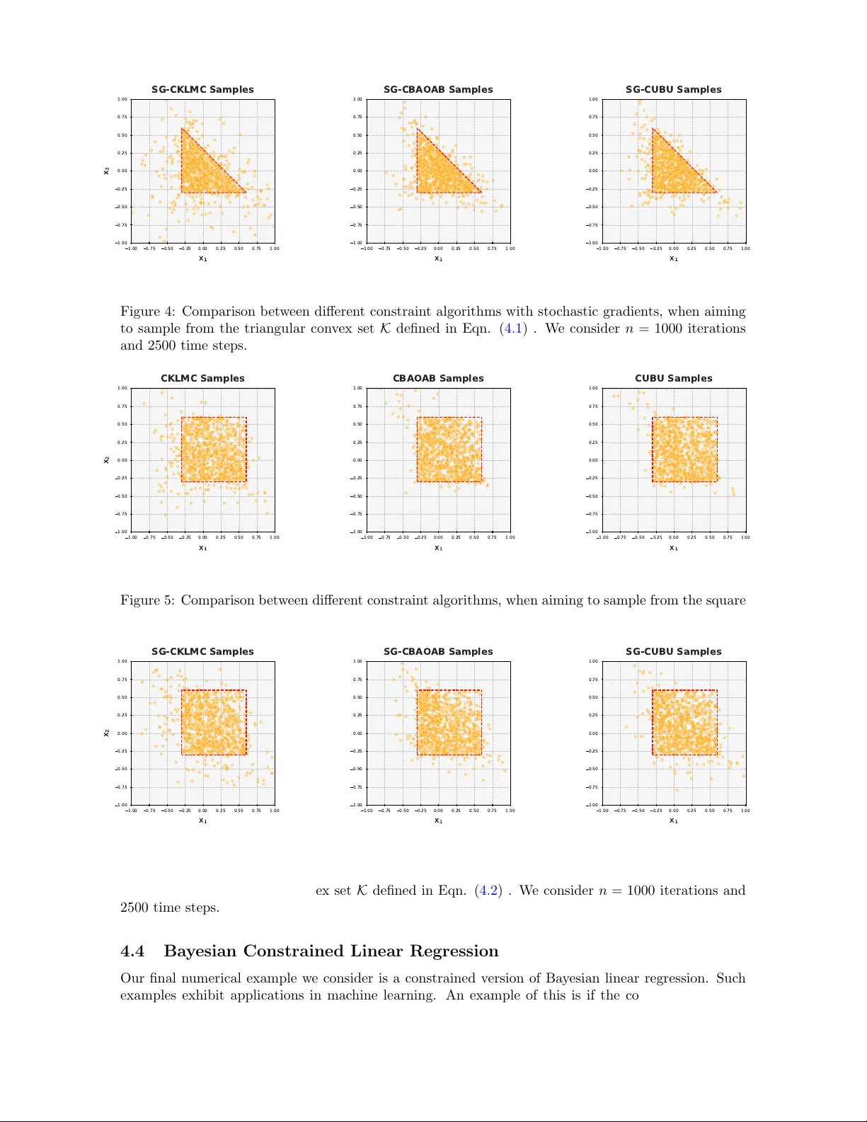
Kinetic Langevin Splitting Sc hemes for Constrained Sampling Neil K. Chada ∗ Lu Y u † Marc h 25, 2026 Abstract Constrained sampling is an imp ortan t and challenging task in computational statistics, con- cerned with generating samples from a distribution under certain constrain ts. There are numerous t yp es of algorithm aimed at this task, ranging from general Mark ov c hain Monte Carlo, to unad- justed Langevin metho ds. In this article we prop ose a series of new sampling algorithms based on the latter of these, speciﬁcally the kinetic Langevin dynamics. Our series of algorithms are mo- tiv ated on adv anced numerical metho ds whic h are splitting order schemes, which include the BU and BAO families of splitting sc hemes.Their adv antage lies in the fact that they ha ve fav orable strong order (bias) rates and computationally eﬃciency . In particular we pro vide a num b er of theoretical insights which include a W asserstein contraction and conv ergence results. W e are able to demonstrate fav orable results, suc h as improv ed complexity b ounds ov er existing non-splitting metho dologies. Our results are veriﬁed through numerical exp eriments on a range of mo dels with constrain ts, which include a toy example and Bay esian linear regression. Keyw ords : Constrained sampling, Splitting schemes, Unadjusted Langevin algorithms, W asserstein complexity Con ten ts 1 In tro duction 2 1.1 F amily of Splitting Schemes . . . . . . . . . . . . . . . . . . . . . . . . . . . . . . . . . . 3 1.2 Other Related W orks . . . . . . . . . . . . . . . . . . . . . . . . . . . . . . . . . . . . . . 5 1.3 Con tributions . . . . . . . . . . . . . . . . . . . . . . . . . . . . . . . . . . . . . . . . . . 5 1.4 Outline . . . . . . . . . . . . . . . . . . . . . . . . . . . . . . . . . . . . . . . . . . . . . 6 1.5 Notation . . . . . . . . . . . . . . . . . . . . . . . . . . . . . . . . . . . . . . . . . . . . . 6 2 Bac kground Material & Algorithms 6 2.1 Constrained Splitting Schemes . . . . . . . . . . . . . . . . . . . . . . . . . . . . . . . . 8 2.2 Extension to Sto chastic Gradients . . . . . . . . . . . . . . . . . . . . . . . . . . . . . . 9 2.3 Con vergence in W asserstein Distance . . . . . . . . . . . . . . . . . . . . . . . . . . . . . 10 3 Main Results 11 3.1 Con vergence Analysis of CUBU . . . . . . . . . . . . . . . . . . . . . . . . . . . . . . . . 11 3.1.1 Extension to SG-CUBU . . . . . . . . . . . . . . . . . . . . . . . . . . . . . . . . 12 3.2 Con vergence Analysis of CBAO AB . . . . . . . . . . . . . . . . . . . . . . . . . . . . . . 13 3.2.1 Extension to SG-CBAO AB . . . . . . . . . . . . . . . . . . . . . . . . . . . . . . 13 3.3 Results for SG-CKLMC . . . . . . . . . . . . . . . . . . . . . . . . . . . . . . . . . . . . 14 ∗ Department of Mathematics, Cit y Universit y of Hong Kong, Hong Kong SAR, neilchada123@gmail.com † Department of Data Science, Cit y Universit y of Hong Kong, Hong Kong SAR, lu.yu@cityu.edu.hk 1 4 Numerical Experiments 16 4.1 Circular Constraint . . . . . . . . . . . . . . . . . . . . . . . . . . . . . . . . . . . . . . . 16 4.2 T riangular Constrain t . . . . . . . . . . . . . . . . . . . . . . . . . . . . . . . . . . . . . 16 4.3 Square Constraint . . . . . . . . . . . . . . . . . . . . . . . . . . . . . . . . . . . . . . . 17 4.4 Ba yesian Constrained Linear Regression . . . . . . . . . . . . . . . . . . . . . . . . . . . 18 5 Conclusion 20 A Pro ofs of Theorems 24 A.1 Proofs of con vergence for CUBU . . . . . . . . . . . . . . . . . . . . . . . . . . . . . . . 24 A.2 Proofs of con vergence for SG-CUBU . . . . . . . . . . . . . . . . . . . . . . . . . . . . . 24 A.3 Proofs of con vergence for CBA OAB . . . . . . . . . . . . . . . . . . . . . . . . . . . . . 25 A.4 Proofs of con vergence for SG-CBA OAB . . . . . . . . . . . . . . . . . . . . . . . . . . . 26 A.5 Proofs of con vergence for SG-CKLMC . . . . . . . . . . . . . . . . . . . . . . . . . . . . 33 B Algorithms 35 1 In tro duction Sampling from probabilit y distributions pla ys a critical role in v arious ﬁelds of science and engineering. Examples of such ﬁelds include n umerical w eather prediction, geophysical sciences, and more recen tly mac hine learning, such as generativ e mo delling or Bay esian neural netw orks [ SSDK21 , HNPSD21 , SD WMG15 ]. Most of these applications exploit Mon te Carlo metho dologies for sampling, with limited, or rarely any signiﬁcan t, restrictions. How ev er, in man y situations it is of interest to consider sampling with dealing with conv ex or compact sets, in other words, restricting the sampling to a particular region within the sample space. W e will refer to this task as c onstr aine d sampling , which will b e the fo cus of this w ork. Many scenarios in v olve sampling on constrained, or conﬁned, spaces, for example sto c hastic optimal con trol and molecular dynamics [ CEAMR12 , LM15 ]. In this con text, the problem in volv es sampling from a probability measure (which we often refer to as the target) ν on suc h sets, whic h are c haracterized b y a densit y function of the form ν ( θ ) = e − U ( θ ) R R p e − U ( θ ) d θ , (1.1) where from the equation, U ( θ ) takes the form U ( θ ) = f ( θ ) + ℓ K ( θ ), where f ( θ ) represen ts a p oten tial function and ℓ K ( θ ) is an indicator function ensuring the parameters θ lies within a conv ex and compact set K ⊂ R p , for p ≥ 1, ℓ K ( θ ) := ( + ∞ if θ / ∈ K 0 if θ ∈ K . (1.2) The absence of smo othness in the target distribution ν presents signiﬁcan t challenges because sam- pling algorithms often depend, quite heavily , on the smo othness prop erties of the target distribution. This is to ensure that one can eﬀectively explore the state space and pro duce representativ e samples of the target ν . Motiv ated by this, we consider the appro ximation for ℓ K of the form ℓ λ K ( θ ) := 1 2 λ 2 d K ( θ ) , where λ > 0 is the tuning parameter and d K : R p → R + is a distance function that quantiﬁes the distance b etw een θ and the constraint set K . W e will later introduce sp eciﬁc c hoices for d K . Now we deﬁne U λ ( θ ) := f ( θ ) + ℓ λ K ( θ ) , (1.3) and the corresp onding surrogate target density ν λ giv en as ν λ ( θ ) := e − U λ ( θ ) R R p e − U λ ( θ ′ ) d θ ′ . (1.4) 2 Therefore, our task at hand is no w to generate samples from the mo diﬁed target, denoted as ν λ ∝ exp( − U λ ), which is designed with constrains through the constrained set K and our p oten tial function ( 1.3 ). Therefore, we consider sampling from the target densit y ν λ ∝ exp( − U λ ). A p opular approac h for this task are kinetic Langevin metho ds. These metho ds are based on the kinetic Langevin dynam- ics (KLD) (also referred to as underdamp ed Langevin dynamics [ CCBJ18 , DRD20 ]), is a well-kno wn approac h to model the dynamics of molecular systems. It has been heavily utilized in diﬀerent math- ematical areas, which include molecular dynamics, Bay esian statistics, and more recen tly mac hine learning. It is deﬁned through tw o coupled pro cesses { L t } t ≥ 0 and { V t } t ≥ 0 whic h are the p osition and the velocity , deﬁned as the follo wing d L t = V t dt, d V t = −∇ U ( L t ) dt − γ V t dt + p 2 γ d W t , (1.5) where U : R p → R is a p otential energy function, { W t } t ≥ 0 is a standard p − dimensional Brownian motion, and γ > 0 is a friction co eﬃcient. Under fairly weak assumptions, the unique in v ariant measure of the pro cess { L t , V t } t ≥ 0 is of the form ν ( d ϑ d v ) ∝ exp  − U ( ϑ ) − ∥ v ∥ 2 2  d ϑ d v . (1.6) An alternative to KLD is to use the ov erdamp ed Langevin dynamics (OLD), which instead just con- siders the pro cess { L t } t ≥ 0 giv en as d L t = −∇ U ( L t ) dt + p 2 β − 1 d W t , (1.7) where β − 1 > 0 is the in verse temp erature parameter. W e notice we ha ve no friction term within ( 1.7 ). The inv ariant measure associated with ( 1.7 ) is deﬁned as ν ( d ϑ ) ∝ exp ( − U ( ϑ )) d ϑ . The beneﬁt of using the KLD ov er the OLD, is that is kno wn to con verge faster to its resp ective in v ariant measure. In the context of Ba yesian sampling, b oth ( 1.5 ) and ( 1.7 ) can b e used to generate samples from a distribution ν . This is ac hieved b y simply setting the p oten tial as the log-p osterior, i.e. U = log ν . Recen t work has lo oked at at connecting these processes, to well-kno wn optimization proce- dures. In order to implement such dynamics, doing so with the full-contin uous pro cess is c hallenging, and often impossible. Therefore one must resort to discretization schemes. The most obvious dis- cretization method is the Euler-Maruyama (EM) scheme, how ev er existing results suggest alternative metho ds, based on the bias, complexity and stabilit y . One such metho d is the randomized midp oin t metho d (RMM) [ SL19 ]. The RMM has also pro vided adv antages in error tolerance and condition n umber dep endence, demonstrated through applications in machine learning [ LJ24 , YY25a , KD24 ]. In the context of constrained sampling, this w as used in the work of Y u et al. [ YY25b ], where they demonstrate sharp er approximation analysis, and improv ed error bounds in terms of W asserstein dis- tance. Despite the success of the RMM applied to constrained sampling, there still remains limitations, suc h as that it uses tw o gradient ev aluations p er time-step. Secondly , for a ﬁxed κ > 0 it is notes that the RMM has a complexity of order O ( ε − 2 / 3 p 1 / 3 ), for dimension p > 0 and ε > 0, which can b e impro ved on. Therefore this promotes the use of p otentially b etter schemes ac hieving improv ements in those asp ects. F or this, w e in tro duce and motiv ate the use of an alternative series of sc hemes referred to splitting order sc hemes. 1.1 F amily of Splitting Sc hemes A p opular choice for solving ODEs are splitting schemes, motiv ated by Gilb ert Strang [ Str63 ], where one splits the dynamics in to diﬀerent components and solv e them individually . This is p ossible due to the fact they can b e in tegrated exactly . This also translates to SDEs whic h include the KLD. W e will introduce tw o family of splitting sc hemes, (i) the BU splitting family , and (ii) the BA O splitting 3 family . F or the former, this w as introduced in [ Zap21 ]. The metho d is based on splitting the SDE ( 1.5 ) as follows  d ϑ d v  =  0 −∇ U ( ϑ ) dt  | {z } B +  v dt − γ v dt + √ 2 γ d W t  | {z } U , whic h can be integrated exactly o v er a step of size h > 0. Given γ > 0, let η = exp ( − γ h/ 2), and for ease of notation, w e deﬁne the following op erators B ( ϑ , v , h ) = ( ϑ , v − h ∇ U ( ϑ )) , (1.8) and U ( ϑ , v , h/ 2 , ξ (1) , ξ (2) ) =  ϑ + 1 − η γ v + r 2 γ  Z (1)  h/ 2 , ξ (1)  − Z (2)  h/ 2 , ξ (1) , ξ (2)  , η v + p 2 γ Z (2)  h/ 2 , ξ (1) , ξ (2)   , (1.9) where Z (1)  h/ 2 , ξ (1)  = r h 2 ξ (1) , Z (2)  h/ 2 , ξ (1) , ξ (2)  = s 1 − η 2 2 γ r 1 − η 1 + η · 4 γ h ξ (1) + r 1 − 1 − η 1 + η · 4 γ h ξ (2) ! . (1.10) The B op erator indicated here is as given previously , whereas U as deﬁned ab ov e is the exact solution in the weak sense of the remainder of the dynamics when ξ (1) , ξ (2) ∼ N (0 , I p ) are indep endent random v ectors. Diﬀeren t palindromic orders of comp osition of B and U can b e taken to deﬁne diﬀeren t n umerical integrators of kinetic Langevin dynamics, tw o such methods are BUB, a half step ( h/ 2) in B , follo wed b y a full step in U and a further half step ( h/ 2) in B and UBU, a half step ( h/ 2) in U follo wed by a full ( h ) B step, follow ed by a half ( h/ 2) U step. The Marko v kernel for an UBU step with stepsize h will b e denoted by P h , whic h can b e describ ed b y ( 1.11 ) as follo ws.  ξ ( i ) k +1  4 i =1 , ξ ( i ) k +1 ∼ N (0 p , I p ) for all i = 1 , ..., 4 . ( ϑ k +1 , v k +1 ) = U B U  ϑ k , v k , h, ξ (1) k +1 , ξ (2) k +1 , ξ (3) k +1 , ξ (4) k +1  = U  B  U  ϑ k , v k , h/ 2 , ξ (1) k +1 , ξ (2) k +1  , h  , h/ 2 , ξ (3) k +1 , ξ (4) k +1  . (1.11) The UBU scheme w as analyzed in [ SSZ21 ], where its adv antages lie in that it only requires one gradien t ev aluation p er iteration but has strong error order of tw o. F urthermore, its stepsize stability analysis, as presented in [ CLPW26 ], is indep endent of dimension p . Other symmetric splitting metho ds are p ossible and hav e b een extensiv ely studied in recen t years. In particular one of them are BAO splitting schemes. The solution maps corresp onding to these parts ma y b e denoted by B , A , and O , which are deﬁned as B = ( ϑ , v − h ∇ U ( ϑ )) , A = ( ϑ + h v , v ) , O = ( ϑ , η 2 v + p 1 − η 4 ξ ) , (1.12) where as b efore η = exp( − γ h/ 2). Examples of such schemes in the BAO family include BAO AB, ABOBA and OBABO schemes [ LM13 , LM15 ], which ha ve the adv antage that they are second order in the weak (sampling bias). The tw o families can b e related through the relationship, breaking the U = A + O . As mentioned, these metho ds are known to attain a weak order of O ( h 2 ). How ever, unlike UBU, they do not attain the same rate for the strong error. A contraction and con vergence analysis w as presen ted, 4 for such schemes, in the following [ LPW24b , LPW24a ], which also includes the extension to sto c hastic gradien ts. Th us far, there has b een no connection in understanding splitting sc hemes for KLD in the context of constrained sampling, which acts as our motiv ation, in the p enalized setting. Before w e discuss our con tributions of this pap er, we provide a brief ov erview of related w ork on constrained sampling using v arious Langevin-based algorithms. 1.2 Other Related W orks The notion of constrained sampling can hav e many diﬀerent in terpretations, depending on the setup and assumptions placed. Our setup, deﬁned brieﬂy thus far through ( 1.4 ), is based on a p enalized constrained setting ﬁrst in tro duced in the w ork of [ GHZ24 ]. Their motiv ation arises from penalty metho ds from con tinuous optimization, which includes a penalty term for constrain t violations. How- ev er, this is not the only setup one could consider for constrained settings. A natural, but diﬃcult setting could be to consider manifolds directly , which require sophisticated mathematical metho ds to eﬀectiv ely sample from the target. Recent w ork that has considered this, in the context of Langevin dynamics, includes [ KL V22 , NDBD24 ]. Some of these w orks require tec hnical couplings, to ensure one can obtain b oth W asserstein con vergence and con traction. F urthermore, m uch of these w orks are based on accept-reject MCMC algorithms like HMC. Despite the elegance of such prop osed work, w e consider a more simpliﬁed setting which is easier to b egin with, b efore moving to a p otential manifold setting in future work. Other such works include [ LST24 ], where the authors dev elop a conﬁned BA O in tegrators for Langevin dynamics. It is the ﬁrst paper aimed at exploiting suc h splitting schemes in the context of a conﬁned space. Ho wev er, it diﬀers in that the dynamics are designed to reﬂect of b oundaries, and the information is enco ded in to each step of the integrator. More recent literature includes that of [ DFT + 25 , CKK24 ], where these pap ers consider a diﬀeren t setup, motiv ated through a primal-dual setting, and whic h do not include a KLD setting, i.e. only one underlying process { L t } t ≥ 0 . 1.3 Contributions W e highligh t our con tributions of this work through the following p oints b elow: • W e introduce new algorithms for the task of constrained sampling based on the task of sampling from ( 1.1 ). Sp eciﬁcally w e introduce ULA-type algorithms, based on splitting order discretization sc hemes, namely UBU and BAO AB. As a result our new algorithms we propose for this work include the CUBU and CBAO AB algorithms. • W e develop a step-size stabilit y analysis for each of the new algorithms discussed abov e. Such an analysis utilizes assumptions on the underlying p otential, such as conv exity and smo othness assumptions, which we will pro vide later in within the document. • W e pro vide a complexity analysis in terms of W asserstein conv ergence, whic h translates to the n umber of steps to achiev e an order of accuracy ε > 0. A summary of our complexity b ounds are pro vided in T able 1 , which highlight the gains and impro vemen t by using splitting schemes, o ver traditional discretization sc hemes. Our results will consider diﬀeren t pro jection methods, whic h include the Bregman and Gauge pro jection. • T o complement the newly developed constrained sampling algorithms, we also pro vide extensions to the case of sto chastic gradients. This will include both SG-CUBU and SG-BAO AB, as w ell as a non-splitting sc heme for comparison, whic h was not previously derived. These are also presen ted in T able 1 , which also demonstrate fa vorable complexit y ov er SG-CKLMC, which w e also consider and pro vide pro ofs, for this work. • Numerical exp eriments are pro vided on a range of problems to demonstrate the performance gains of the constrained splitting sc hemes. This will include a to y problem, with constrain ts deﬁned through b oth a triangle and circle, and a more adv anced numerical example of Ba yesian logistic regression. F or each example we compare our newly developed algorithms to existing ones. 5 Algorithm Complexit y Reference Metric Pro jection CLMC (PULMC) O ( ε − 7 ) [ GHZ24 ] W 2 Euclidean CKLMC O ( ε − 4 ) [ YY25b ] W 2 Euclidean CUBU O ( ε − 3 ) This w ork, Theorem 3.1 W 1 Bregman, Gauge CUBU O ( ε − 3 ) This w ork, Theorem 3.1 W 2 Bregman, Gauge CBA OAB O ( ε − 3 ) This w ork, Theorem 3.3 W 1 Bregman, Gauge CBA OAB O ( ε − 3 ) This w ork, Theorem 3.3 W 2 Bregman, Gauge SG-CUBU O ( ε − 6 ) This w ork, Theorem 3.2 W 1 Bregman, Gauge SG-CUBU O ( ε − 21 / 2 ) This work, Theorem 3.2 W 2 Bregman, Gauge SG-CBA OAB O ( ε − 7 ) This w ork, Theorem 3.4 W 1 Bregman, Gauge SG-CBA OAB O ( ε − 25 / 2 ) This work, Theorem 3.4 W 2 Bregman, Gauge SG-CKLMC O ( ε − 18 ) This work, Theorem 3.6 W 2 Bregman, Gauge T able 1: T able of comparison b etw een diﬀerent discretization schemes for constrained KLD, in terms of their complexity . Our improv ed rates are highligh ted in red. 1.4 Outline The outline of this paper is as follows, we will b egin with Section 2 , which will pro vide an o verview of the material needed for the latter sections. This will include a discussion on assumptions w e will use based on the potential and densit y function, and the in tro duction of our constrained splitting order sc hemes. This will lead onto Section 3 where we presen t our main theoretical ﬁndings which include b oth a step-size stability analysis and W asserstein complexity b ounds. W e will defer the proofs to App endix A . T o verify our theoretical results, we will introduce our numerical sim ulations in Section 4 demonstrating improv ements under our new metho ds, where w e conclude our ﬁndings in Section 5 . W e also present our new methods in algorithmic form in App endix B . 1.5 Notation Denote the p -dimensional Euclidean space by R p . W e use θ for deterministic vectors and ϑ for random vectors. F or symmetric matrices A and B , w e write A ≼ B (or B ≽ A ) if B − A is p ositive semi-deﬁnite. F or a measurable function f : R p → R and a set K ⊂ R p , deﬁne the oscillation osc K ( f ) := sup x ∈K f ( x ) − inf x ∈K f ( x ) . F or a twice diﬀerentiable function f , we denote its gradient and Hessian b y ∇ f and ∇ 2 f , resp ectiv ely . δ x denotes the Dirac measure concentrated at the p oin t x . 2 Bac kground Material & Algorithms In this section we provide a primer on the necessary background material b efore discussing our main results. This includes v arious assumptions required on the p otential function, and on the compact set K . After-whic h, we will introduce our new constrained algorithms which w e refer to as CUBU and CBA OAB. This will b e then b e considered for sto chastic gradients. All algorithms ar expressed in algorithmic form in the app endices. W e b egin this section b y assuming the conv ex and compact set K satisﬁes the follo wing assumptions. Assumption 2.1. Given c onstants 0 < r < R < ∞ , it holds that B 2 ( r ) ⊂ K ⊂ B 2 ( R ) , wher e B 2 ( r ) denotes the Euclide an b al l of r adius r c enter e d at the origin. Moreo ver, we imp ose the following assumption on the functions f and d K . Assumption 2.2. The function f : R p → R attains its glob al minimum at the origin. Assumption 2.3. Ther e exists some c onstants 0 < c 1 ⩽ c 2 such that c 1 ∥ θ − P K ( θ ) ∥ 2 2 ⩽ d K ( x ) ⩽ c 2 ∥ θ − P K ( θ ) ∥ 2 2 , 6 wher e P K : R p → R p is a pr oje ction op er ator onto set K . Mor e over, d K ( θ ) ⩾ 0 for al l θ ∈ R p , and d K ( θ ) = 0 whenever θ ∈ K . Let us brieﬂy discuss each of the abov e assumptions. Assumption 2.1 is important and has been made in the v arious w orks in the area of constrained sampling [ BDMP17 , GHZ24 ]. Assumption 2.2 is made to ensure a conv ergence analysis can b e pro vided, with con vexit y . Finally Assumption 2.3 is an assumption on the distance function, which ensures the potential U λ inherits smo othness and strong con vexit y from f . Related to Assumption 2.3 , w e no w in tro duce t wo choices of ℓ K , based on commonly used pro jection classes, whic h are the Bregman and the Gauge pro jection. These pro jections ha ve b een widely used in v arious machine learning applications, whic h include clustering and detection of outliers [ XNZ08 , Gho19 ]. W e state this b elo w. Example 2.1 (Bregman pro jection) . Consider the Br e gman pr oje ction P B K : R p → K , deﬁne d as P B K ( θ ) := argmin θ ′ ∈K ( θ − θ ′ ) ⊤ Q ( θ − θ ′ ) , such that Q ∈ R p × p is a p ositive semi-deﬁnite symmetric matrix. Example 2.2 (Scaling-based pro jection) . Consider the Gauge pr oje ction P G K : R p → K , deﬁne d as P G K := θ g K ( θ ) , such that g K is a variant of the Gauge function, which is asso ciate d with the set K , given as g K ( θ ) := inf { t ≥ 1 : θ ∈ t K} . W e remark that the Bregman distance is equiv alent to the squared Mahalanobis distance, deﬁned as F ( θ ) = 1 2 θ ⊤ Q θ . Therefore, we can consider a distance function of the form d K ( θ ) = ∥ θ − P B K ( θ ) ∥ 2 2 . As as a result The Bregman pro jection, can b e written as ℓ B , θ K ( θ ) = 1 2 λ 2 ∥ θ − P B K ( θ ) ∥ 2 2 = inf θ ∈ R p  ℓ K ( θ ′ ) + 1 2 λ 2 ( θ − θ ′ ) ⊤ Q ( θ − θ ′ )  . Let us now place a num b er of common, and imp ortant, assumptions on f as well the p otential U λ , which can b e found b elow. These assumptions are crucial for our error analysis, and step-size stabilit y analysis. They are mostly generic assumptions used within the literature of sampling as an optimization pro cedure [ Che25 ]. Assumption 2.4. The function f : R p → R is twic e c ontinuously diﬀer entiable, and m -str ongly c onvex, that is, f ( θ ′ ) ⩾ f ( θ ) + ⟨∇ f ( θ ) , θ ′ − θ ⟩ + m 2 ∥ θ − θ ′ ∥ 2 . Mor e over, f is L -smo oth, which satisﬁes the fol lowing ∥∇ f ( θ ) − ∇ f ( θ ′ ) ∥ ⩽ L ∥ θ − θ ′ ∥ , ∀ , θ , θ ′ ∈ R p , wher e m > 0 and L > 0 ar e the str ong c onvex, and Lipschitz, c onstants. As sho wn in Lemmas 12 and 13 from [ YY25b ], the surrogate p otential U λ inherits the smo othness and strong con vexit y of f , provided that the distance function d K satisﬁes Assumption 2.3 . More sp eciﬁcally , U λ is m -stronlgy conv ex and M λ -smo oth with M λ = L + 1 λ 2 C pro j , where the constan ts C pro j > 0 dep ends on the sp eciﬁc choice of the pro jection operator. In this work, w e fo cus on the Bregman pro jection and the Gauge pro jection in tro duced in [ YY25b ], for which C pro j can b e taken as a universal p ositive constant. F urthermore, we require that U λ satisﬁes the following assumption. 7 Assumption 2.5 (Lipschitz Hessian) . Assume b oth the function f : R p → R and the surr o gate p otential U λ : R p → R p ar e thr e e times diﬀer entiable. Supp ose ther e exist c onstants L 1 , M λ 1 > 0 such that, for any θ ∈ R p and arbitr ary w 1 , w 2 ∈ R p , ∥ H ′ f ( θ )[ w 1 , w 2 ] ∥ ⩽ L 1 ∥ w 1 ∥∥ w 2 ∥ , ∥ H ′ λ ( θ )[ w 1 , w 2 ] ∥ ⩽ M λ 1 ∥ w 1 ∥∥ w 2 ∥ , wher e H f : R p → R p × p and H λ : R p → R p × p denotes the Hessian of f and U λ , r esp e ctively. W e note that the constan t M λ 1 dep ends on the geometry of the constraint set K , and and the parameter λ en ters the b ound through M λ 1 . Consider Example 2.1 with Q = I , whic h corresp onds to the Euclidean pro jection. In this case, the distance function simpliﬁes to d K ( θ ) = ∥ θ − P B K ( θ ) ∥ 2 2 . Example 2.3 (Ellipsoid) . Consider the el lipsoidal c onstr aint K = { θ ∈ R p : θ ⊤ A θ ⩽ 1 } , A = A ⊤ ≻ 0 , wher e the matrix A has minimum and maximum eigenvalues denote d by λ min and λ max , r esp e ctively. Then we have the fol lowing c onstant M λ 1 = L 1 + 4 λ 2  λ max λ min  3 . Example 2.4 ( ℓ q -ball with q > 2) . Consider the c onstr aint K = { θ ∈ R p : ∥ θ ∥ q ⩽ 1 } Then we have the fol lowing c onstant M λ 1 = L 1 + 8 λ 2 p 3 / 2 ( q − 1) 2 . 2.1 Constrained Splitting Sc hemes Let us introduce our ﬁrst constrained algorithm which we refer to as c onstr aine d-UBU , or abbreviated to CUBU. The form of the splitting is in the same spirit as UBU [ SSZ21 ], with the key diﬀerence of the B -operator, which is deﬁned as B c ( ϑ , v , h ) = ( ϑ , v − h ∇ U λ ( ϑ )) , (2.1) for h > 0, whic h includes the p otential U λ ( ϑ ) giv en as ( 1.9 ), and where the U op erator remains the same as b efore, i.e. U ( ϑ , v , h/ 2 , ξ (1) , ξ (2) ) =  ϑ + 1 − η γ v + r 2 γ  Z (1)  h/ 2 , ξ (1)  − Z (2)  h/ 2 , ξ (1) , ξ (2)  , η v + p 2 γ Z (2)  h/ 2 , ξ (1) , ξ (2)   , with similar deﬁnitions of Z (1) and Z (2) pro vided through Eqn. ( 1.10 ). The acceleration of UBU requires the surrogate function U λ to b e smo oth and strongly conv ex. This requiremen t is satisﬁed under Assumption 2.3 , pro vided that f is strongly con vex and smo oth. The b ounded third deriv ative condition, as stated in Assumption 3 of [ SSZ21 ], requires an additional assumption on the b oundary of the constraint set K . Algorithm 1 in the app endix provides an algorithmic form of the CUBU. T o establish the conv ergence of UBU under constraints, we need the following results by Theorems 23 and 25 from [ SSZ21 ]. W e no w extend the existing W asserstein conv ergence result of UBU to CUBU, pro vided b elow. 8 Theorem 2.1. Under Assumptions 2.4 - 2.5 ,(Assumption 1-3 in [ SSZ21 ]), and setting γ = 2 , it holds for a smal l h > 0 that W 2 ( ν λ , ν UBU n ) ⩽  1 − mh 3 M λ  n W 2 ( ν λ , ν UBU 0 ) +  1 √ M λ + C 1 M λ 1 ( M λ ) 2  κ √ ph 2 . wher e C 1 is a universal c onstant. The exact notion of Wasserstein c onver genc e, and the W 2 metric wil l b e pr ovide d in Se ction 2.3 . Our ﬁnal constrained splitting scheme w e in tro duce is the c onstr aine d-BAO AB , abbreviated to CBA OAB. In this setup, we now mo dify our original mappings as now B = ( ϑ , v − h ∇ U λ ( ϑ )) , A = ( ϑ + h v , v ) , O = ( ϑ , η 2 v + p 1 − η 4 ξ ) , (2.2) for λ > 0, arising from Eqn. ( 1.3 ). Algorithm 2 in the app endix provides an algorithmic form of the CBA OAB. Remark 2.2. We r emark ther e ar e other existing splitting schemes, b ase d on the BA O family for the KLD. These include OBABO and ABOBA. Our r e ason for c onsidering only BAO AB, is r elate d to its impr ovement in terms of the we ak err or (also asymptotic bias), which is of or der 2, and that it has no bias when aiming to sample fr om Gaussian tar gets. Extending this, pr ovides no additional diﬃculties but would pr olong the p ap er with very similar te dious c alculations. Ther efor e we c onsider this for p otential futur e work. 2.2 Extension to Stochastic Gradients F or man y practical scenarios, the exact computation of the p otential can b e diﬃcult, or time-consuming, esp ecially for high-dimensions. As a result, we consider the use of sto chastic gradien ts (SG), which instead do not require the full ev aluation of ∇ U λ ( θ ). The form of our SG-based metho ds we consider, are based on the notion of mini-batching. In order to consider SG v ariants, we require a deﬁnition of our inexact gradient, which is given b elow. Deﬁnition 2.1. A sto chastic gr adient appr oximation of a p otential f is deﬁne d by a function G : R p × Ω → R p and a pr ob ability distribution ρ on a Polish sp ac e Ω , such that for every θ ∈ R p , G ( θ , · ) is me asur able on (Ω , F ) , and for ω ∼ ρ , E ( G ( θ , ω )) = ∇ f ( θ ) . The function G and the distribution ρ to gether deﬁne the sto chastic gr adient, which we denote as ( G , ρ ) . As w e are considering a sto chastic gradient, one p ossibilit y is to directly add noise to the gradien t, whic h is written as ( G , ρ ) = ∇ f ( θ ) + ξ , where ξ ∼ N (0 , 1) is a random normal p erturbation. Then, we can place the follo wing assumptions on the sto chastic gradien t. Assumption 2.6. L et us assume we have a sto chastic (or noisy) gr adient deﬁne d thr ough Deﬁnition 2.1 , then we have the fol lowing assumptions. (i) ( G , ρ ) is an unbiase d estimate of ∇ f ( θ ) (unbiase d gr adient). (ii) E h    ( G , ρ ) − ∇ f ( θ )    2    θ i ⩽ σ 2 1 L 2 ( ∥ θ ∥ 2 ) (b ound on the sto chastic gr adient). (iii) E h    ∇ θ ( G , ρ ) − ∇ 2 f ( θ )    2    θ i ⩽ σ 2 2 (b ound on the se c ond derivative). In practice, the p oten tial function f often takes the form f ( θ ) = n X i =1 f i ( θ ) . 9 Accordingly , the sto c hastic gradien t of f is typically computed as ˜ ∇ f ( θ ) = 1 b X j ∈ Ω f j ( θ ) , where Ω ⊂ { 1 , . . . , n } is a mini-batc h of size b . In this setting, we hav e σ 2 1 = O (1 /b ) and σ 2 2 = O (1 /b ). Sto c hastic gradient v ersions of BAO AB and UBU ha ve b een analyzed, and discussed in a series of w orks, i.e. [ CLPW26 , LPW24a ], whic h discuss contraction rates and non-asymptotic conv ergence in the W asserstein metric. Later we will use some of these results, to establish similar results in the constrained setting. In our setup, we provide t wo additional algorithms, the SG-CUBU and SG- BA OAB, which are also pro vided in Algorithms 1 and 2 . W e do not state the full algorithms for for the full-gradient versions, to a void rep etition, but follo w v ery similarly . W e brieﬂy remark that Assumption 2.6 contains sub-assumptions that will b e sp eciﬁc to diﬀerent SG algorithms. 2.3 Conv ergence in W asserstein Distance In order to v erify our error b ounds, we require a suﬃcien t metric. W e will consider the W asserstein distance, whic h is a p opular metric to sho w conv ergence of sampling algorithms. In particular, w e will focus on W asserstein contraction [ EGZ19 , Dal17 ]. The key underlying idea is that if one sho ws con traction b etw een tw o measures, then this implies a unique inv arian t measure and conv ergence to wards it. The general setup of these results follow from W q ( ν 0 P n h , ν ) ≤ W q ( ν 0 P n h , ν λ ) | {z } sampling error + W q ( ν λ , ν ) | {z } approxiam tion error , where ν 0 is some initial measure, P n h is a Mark ov transition k ernel based on some algorithm with step-size h > 0 after n -steps, and ν is the target measure. Pro viding b ounds of the form, translates to ho w many n -steps are required to achiev e an accuracy of ε , for ε > 0. Belo w we provide the deﬁnition of the W asserstein distance, whic h is required, b efore stating our ﬁrst result whic h is a prop osition. Deﬁnition 2.2 ( q -W asserstein distance) . L et us deﬁne P q ( R 2 p ) to b e the set of pr ob ability me asur es which have q -th moment for q ∈ [1 , ∞ ) (i.e. E ( ∥ Z ∥ q ) < ∞ ). Then the q -Wasserstein distanc e, b etwe en two me asur es ν, ν ′ ∈ P q ( R 2 p ) , is deﬁne d as W q ( ν, ν ′ ) =  inf ξ ∈ Γ( ν ,ν ′ ) Z R p × R p ∥ z 1 − z 2 ∥ q 2 dξ ( z 1 , z 2 )  1 /q , (2.3) wher e ∥ · ∥ 2 is the norm we c onsider, and Γ( ν, ν ′ ) is the set of me asur es with r esp e ctive mar ginals of ν and ν ′ , wher e the inﬁmum is over al l c ouplings ξ . W e now state our ﬁrst result, whic h is an upp er W asserstein b ound b etw een our target measure ν and its corresp onding approximation ν λ , based on the splitting schemes we ha ve discussed. Such a result demonstrates that W q ( ν, ν λ ) → 0 as λ → 0. Prop osition 2.1. Under Assumptions 2.1 - 2.3 , for any q ⩾ 1 and any λ satisfying 0 < λ <  √ c 1 r p + q ^ √ c 1 r e osc K ( f ) 3 √ π V ol( K ) p  , it holds that W q ( ν, ν λ ) ⩽ C ( p, q ) ·      λ, 1 /p + 1 /q > 1 , λ log 1 /q ( 1 λ ) , 1 /p + 1 /q = 1 , λ 1 /p +1 /q , 1 /p + 1 /q < 1 10 wher e C ( p, q ) = C 0 " p · e 4 osc K ( f ) c 1 / 2 1 ·  max( R, 1) min( r , 1)  (2 p +1) # 1 /p +1 /q , and C 0 > 0 is a universal c onstant, and r e c al ling osc K ( f ) is deﬁne d in Subse ction 1.5 . If we analyze Prop osition 2.1 ab ov e, w e hav e a phase transition of the W asserstein b ound, that dep ends on b oth the dimension p and and the order q . The ab ov e result is very similar to that of [ YY25a ], with the modiﬁcation being from the altered constant C ( p, q ), and the tuning parameter λ > 0. W e will use this proposition for our conv ergence analysis in Section 3 . Remark 2.3. Befor e we discuss our main r esults, we would like to r efer to T able 1 , which pr ovides a c omplexity analysis of our diﬀer ent algorithms. By CLMC (PULMC) we r efer to the OLD, which is discr etize d by the Euler-Maruyama scheme, and similarly for CKLMC using the KLD. Complexity r esults of b oth have b e en pr oven, and we state them in the table as a p oint of c omp arison with our pr op ose d splitting schemes. 3 Main Results In this section w e provide our main results of the in tro duced constrained algorithms, from the previous section. In particular w e will provide a series of con vergence results based on the W asserstein com- plexit y deﬁned in Subsection 2.3 . This will be done for CUBU, CBAO AB, their SG versions and also the SG-CKLMC, which utilizes the Euler-Maruy ama discretization of the KLD. Finally , w e pro vide a complexit y analysis, in terms of the num b er of iterations to acquire a certain level of accuracy for each algorithm. W e b egin by ﬁrst discussing CUBU. All pro ofs will b e deferred to the App endix. 3.1 Conv ergence Analysis of CUBU Theorem 3.1 (Con vergence of CUBU) . Under Assumptions 2.1 - 2.5 , set γ = 2 . Supp ose that λ is suﬃciently smal l and satisﬁes 0 < λ <  √ c 1 r p + 2 ^ √ c 1 r e osc K ( f ) 3 √ π V ol( K ) p  . Then, for an y suﬃciently smal l step size h > 0 and any p > 2 , it holds that W 2 ( ν, ν UBU n ) ⩽ e − mhn 3 M λ W 2 ( ν, ν UBU 0 ) +  1 √ M λ + C 1 M λ 1 ( M λ ) 2  κ √ ph 2 + C ( p, 2) λ 1 2 + 1 p . Mor e over, when the initial p oint θ UBU 0 = 0 and v UBU 0 ∼ N p (0 , I p ) , it holds that W 1 ( ν, ν UBU n ) ⩽ e − mhn 3 M λ r p m +  1 √ M λ + C 1 M λ 1 ( M λ ) 2  κ √ ph 2 + C ( p, 1) λ . Her e, κ = M λ /m, C 1 > 0 is a universal c onstant sp e ciﬁe d in The or em 2.1 , and C ( p, q ) is deﬁne d in Pr op osition 2.1 . F or b oth Gauge pro jection and Euclidean pro jection, we adopt M λ = O (1 /λ 2 ) , M λ 1 = O (1 /λ 2 ) corresp onding to Example 2.3 and Example 2.4 . The preceding theorem implies the follo wing corollary . Corollary 3.1. L et err or level ε ∈ (0 , 1) b e smal l. (a) We set λ = Θ( h 4 p 3 p +2 ) , and cho ose h > 0 , with n ∈ N + , such t hat h = O  ε 3 p +2 2 p +4  , n = ˜ Ω  ε − 11 p +2 4+2 p  , then we have that W 2 ( ν CUBU n , ν ) = ˜ O ( ε ) . 11 (b) We set λ = Θ( h ) , and cho ose h > 0 , with n ∈ N + , such t hat h = O ( ε ) , n = ˜ Ω  ε − 3  , then we have that W 1 ( ν CUBU n , ν ) = ˜ O ( ε ) . The num b er of iterations required by the CUBU algorithm to achiev e W 2 ( ν, ν CUBU n ) ⩽ ε is of order O ( ε − 11 p +2 4+2 p ), When p > 2, w e note that 11 p +2 2 p +4 ⩾ 5 . 5 − 10 2 p . Moreov er, the num b er of iterations required to ac hieve W 1 ( ν, ν CUBU n ) ⩽ ε is of order O ( ε − 3 ). By direct comparison with other methods based on Euler–Maruy ama discretization (see T able 1 ), we observe an impro vemen t in iteration complexit y . 3.1.1 Extension to SG-CUBU No w we focus on the CUBU algorithm with gradients, referred to as SG-CUBU. In the following theorem, we quantify the W asserstein-1 and W asserstein-2 distances b et ween the distribution of the output of the SG-CUBU algorithm and the target density ν . Theorem 3.2. Under Assumptions 2.1 - 2.4 and Assumption 2.6 , supp ose that λ satisﬁes 0 < λ < √ c 1 r p + 2 ^ √ c 1 r e osc K ( f ) 3 √ π V ol( K ) p ! . Then, for an y p > 2 , γ ⩾ √ 8 M λ and the step size 0 < h <  mM λ 4 γ σ 2 2 ^ 1 2 γ  , it holds that W 2 ( ν SG − CUBU n , ν λ ) ⩽  1 − mh 8 γ  n/ 2 W 2 ( ν SG − CUBU 0 , ν ) + 2 γ √ h m s σ 2 1 L 2 √ M λ  h 2 ( M λ ) 2 d m 2 + d m  + √ d ( √ M λ + γ ) h 2 + 2 C ( p, 2) λ 1 /p +1 / 2 . Mor e over, when initialize the algorithm with ϑ SG − CUBU 0 = 0 , and v SG − CUBU 0 ∼ N p (0 , I p ) , it fol lows that W 1 ( ν SG − CUBU n , ν ) ⩽  1 − mh 8 γ  n/ 2 r p m + 2 γ √ h m s σ 2 1 L 2 √ M λ  h 2 ( M λ ) 2 d m 2 + d m  + √ d ( √ M λ + γ ) h 2 + C ( p, 1) λ . M λ = O (1 /λ 2 ) in the previously stated theorem, w e obtain the following corollary . Corollary 3.2. L et the err or level ε ∈ (0 , 1) b e smal l, and set γ = √ 8 M λ . (a) Cho ose λ = Θ( h ) , and set h > 0 , the b atch size and the numb er of iter ations b, n ∈ N + such that h = O  ε 2 p p +2  , b = Ω  ε − 6 p +4 p +2  , n = ˜ Ω  ε − 4 p p +2  , then we have that W 2 ( ν SG − CUBU n , ν ) = ˜ O ( ε ) . (b) Set λ = Θ( h ) , and cho ose h > 0 , with the b atch size and the numb er of iter ations b, n ∈ N + , such that h = O ( ε ) , b = Ω  ε − 4  , n = ˜ Ω  ε − 2  , then we have that W 1 ( ν SG − CUBU n , ν ) = ˜ O ( ε ) . The num b er of gradient ev aluations required by the SG-CUBU algorithm to achiev e W 2 ( ν, ν SG − CUBU n ) ⩽ ε is of order O ( ε − 10 p +4 p +2 ), When p > 2, w e note that 10 p +4 p +2 ⩾ 10 p +20 p +2 − 16 p +2 . Moreov er, the n umber of gradien t ev aluations required to achiev e W 1 ( ν, ν SG − CUBU n ) ⩽ ε is of order O ( ε − 6 ). 12 3.2 Conv ergence Analysis of CBAO AB Let us now extend our results and setup to the methodology of constrained BAO AB, i.e. CBAO AB. The following theorem presents the conv ergence results of the BA OAB scheme under constrain ts. Theorem 3.3. Under Assumptions 2.1 - 2.5 , assume that λ satisﬁes 0 < λ < √ c 1 r p + 2 ^ √ c 1 r e osc K ( f ) 3 √ π V ol( K ) p ! . Then, for an y p > 2 , γ ⩾ 2 √ M λ and the step size h is chosen as 0 < h <  1 − e − γ h 4 √ M λ ^ 4 γ m  , it holds that W 2 ( ν CBAO AB n , ν ) ⩽ 21 e − mh ( n − 1) 4 γ W 2 ( ν CBAO AB 0 , ν ) + 66000 √ M λ m  4 p M λ p + 3 M λ 1 p M λ  γ h 2 + C ( p, 2) λ 1 / 2+1 /p . Mor e over, when the initial p oint ϑ CBAO AB 0 = 0 and v CBAO AB 0 ∼ N p (0 , I p ) , it holds that W 1 ( ν CBAO AB n , ν ) ⩽ 21 e − mh ( n − 1) 4 γ r p m + 66000 √ M λ m  4 p M λ p + 3 M λ 1 p M λ  γ h 2 + C ( p, 1) λ . wher e C ( p, 1) and C ( p, 2) ar e given in Pr op osition 2.1 . Setting M λ 1 = O (1 /λ 2 ) , M λ = O (1 /λ 2 ) in the previously stated theorem, we obtain the following corollary . Corollary 3.3. L et the err or level ε ∈ (0 , 1) b e smal l. (a) Set λ = Θ( h 4 p/ (7 p +2) ) , and cho ose h > 0 and the numb er of iter ations n ∈ N + so that h = O  ε 7 p +2 2 p +4  , n = e Ω  ε − 11 p − 2 2 p +4  , then we have W 2 ( ν CBAO AB n , ν ) = e O ( ε ) . (b) Set λ = Θ( h 1 / 2 ) , and cho ose h > 0 and the numb er of iter ations n ∈ N + so that h = O  ε 2  , n = e Ω  ε − 3  , then we have W 1 ( ν CBAO AB n , ν ) = e O ( ε ) . A comparison b et ween the iteration complexities of the CBA OAB metho d in this corollary and the CUBU metho d in Corollary 3.1 sho ws that they are of the same order, diﬀering only b y constant factors. 3.2.1 Extension to SG-CBA O AB As done before, we consider the additional extension of CBAO AB to that of sto chastic gradien ts, which results in a new algorithm entitled SG-CBA OAB. Belo w we presen t a main conv ergence result and a corollary that details the computational complexity . Theorem 3.4. Under Assumptions 2.1 - 2.6 , supp ose that λ satisﬁes 0 < λ < √ c 1 r p + 2 ^ √ c 1 r e osc K ( f ) 3 √ π V ol( K ) p ! . 13 Then, for an y p > 2 , γ ⩾ √ 8 M λ and the step size 0 < h <  1 − e − γ h 2 √ M λ ^ 4 γ m ^ 1 ^ 1 4 γ  , it holds that W 2 ( ν SG − CBAO AB n , ν λ ) ⩽ 4(1 − e − γ h ) m K noise ( h ) + (1 − ρ ( h )) n  W 2 ( ν SG − CBAO AB 0 , ν λ ) + C bias h (1 − e − γ h )  + C bias h (1 − e − γ h ) + 2 C ( p, 2) λ 1 /p +1 / 2 . Mor e over, when initialize the algorithm with ϑ SG − CBAO AB 0 = 0 , and v SG − CBAO AB 0 ∼ N p (0 , I p ) , it fol lows that W 1 ( ν SG − CBAO AB n , ν λ ) ⩽ 4(1 − e − γ h ) m K noise ( h ) + (1 − ρ ( h )) n  r p m + C bias h (1 − e − γ h )  + C bias h (1 − e − γ h ) + C ( p, 1) λ . Her e, ρ ( h ) = mh 2 4(1 − e − γ h ) , C bias and K noise ar e explicit c onstants that ar e pr ovide d in Pr op osition A.1 . Corollary 3.4. L et the err or level ε ∈ (0 , 1) b e suﬃciently smal l. (a) Set λ = Θ  h 4 p 7 p +2  , and cho ose the step size h > 0 , b atch size b ∈ N + , and numb er of iter ations n ∈ N + so that h = O  ε 7 p +2 2 p +4  , b = Ω  ε − 7 p +2 p +2  , n = e Ω  ε − 11 p +2 2 p +4  . Then we have W 2 ( ν SG − CBAO AB n , ν ) = O ( ε ) . (b) Set λ = Θ  h 1 / 2  , and cho ose the step size h > 0 , b atch size b ∈ N + , and numb er of iter ations n ∈ N + so that h = O  ε 2  , b = Ω  ε − 4  , n = e Ω  ε − 3  . Then we have W 1 ( ν SG − CBAO AB n , ν ) = O ( ε ) . The conclusion from the following corollary , is that the num b er of gradient ev aluations required to ac hieve W 2 ( ν, ν SG − CBAO AB n ) ⩽ ε is of order O ( ε − 25 p +6 2 p +4 ). Similarily , the num b er of gradien t ev aluations required to achiev e W 1 ( ν, ν SG − CBAO AB n ) ⩽ ε is of order O ( ε − 7 ). Remark 3.5. We r emark that unlike the ful l-gr adient c ase, the c omplexity r esults of SG-CBAO AB ar e worse than SG-CUBU. The slower c onver genc e r ate is mainly due to the additional B-step, which brings in extr a sto chastic-gr adient err or. This additional err or term le ads to a less favor able over al l err or b ound, me aning that BAO AB with sto chastic gr adients ne e ds mor e gr adient evaluations than sto chastic-gr adient UBU to attain the same level of ac cur acy. 3.3 Results for SG-CKLMC Thanks to our reﬁned analysis of the distance betw een the smooth surrogate and the target distribution, w e are able to derive a tigh ter upp er b ound on the conv ergence rate of CKLMC with sto chastic gradien ts (referred to as SG-CKLMC), as stated in the following theorem. Theorem 3.6. Under Assumptions 2.1 – 2.4 and Assumption 2.6 (i)–(ii), assume that λ satisﬁes 0 < λ <  √ c 1 r p + 2 ^ √ c 1 r e osc K ( f ) 3 √ π V ol( K ) p  . 14 Then, for an y γ ⩾ √ m + M λ , and any step size h such that 0 < h < min  γ τ 2 K 1 , 2 γ τ , 1 10 γ , m 4 γ M λ  . It holds that W 2 ( ν SG − CKLMC n , ν ) ⩽  1 − 0 . 75 mh γ  n W 2 ( ν SG − CKLMC 0 , ν ) + √ 2 M λ h √ p m + 2 C ( p, 2) λ 1 / 2+1 /p + 8 √ 2 σ 1 L mγ r C V 1 − 2 τ . Her e, the c onstants τ and K 1 ar e deﬁne d by τ = 1 2 min  1 4 , m M λ + γ 2 / 2  , K 1 = max ( 16  ( M λ ) 2 + 2 γ ( M λ ) 2 + σ 2 1 L 2  (1 − 2 τ ) γ 2 , 4 M λ + 2 γ 2 (1 − τ ) + 8 γ 1 − 2 τ ) . The c onstant C V is given by C V = Z R 2 p V ( ϑ , v ) µ 0 ( d ϑ , d v ) + 4 τ  p + mf (0) 2 M λ + γ 2  , wher e the Lyapunov function V is deﬁne d as V ( ϑ , v ) = U λ ( ϑ ) + γ 2 4 ( ∥ ϑ + γ − 1 v ∥ 2 + ∥ γ − 1 v ∥ 2 − τ ∥ ϑ ∥ 2 ) . Mor e over, when the initial p oint θ SG − CKLMC 0 = 0 and v SG − CKLMC 0 ∼ N p (0 , I p ) , it h olds that W 1 ( ν SG − CKLMC n , ν ) ⩽  1 − 0 . 75 mh γ  n r p m + √ 2 M λ h √ p m + 8 √ 2 σ 1 L mγ r C V 1 − 2 τ + C ( p, 1) λ . Adopting M λ = O (1 /λ 2 ) in the previously stated theorem, w e obtain the following corollary . Corollary 3.5. L et the err or level ε ∈ (0 , 1) b e smal l. (a) Set λ = Θ( h 1 / 4 ) , and cho ose h > 0 , the b atch size and the numb er of iter ations b, n ∈ N + so that h = O  ε 8 p p +2  , b = Ω( ε − 8 p p +2 ) , n = e Ω  ε − 10 p p +2  , then we have W 2 ( ν SG − CKLMC n , ν ) = e O ( ε ) after nb sto chastic gr adient evaluations. (b) Set λ = Θ( h 1 / 4 ) , and cho ose h > 0 , the b atch size and the numb er of iter ations b, n ∈ N + so that h = O  ε 4  , b = Ω( ε − 4 ) , n = e Ω  ε − 5  , then we have W 1 ( ν SG − CKLMC n , ν ) = e O ( ε ) after nb sto chastic gr adient evaluations. By direction comparison, with the results from Corollary 3.2 , we notice the SG-CKLMC has worse complexit y rate, esp ecially related to b , where for SG-CUBU it is of order O (1). Therefore in b oth cases of full and sto chastic gradients, the constrained splitting schemes oﬀer fa vorable results. Remark 3.7. We would like to r emark that despite the favor able c omplexity of our c onstr aine d split- ting schemes, the c onstr aine d algorithm of the r andomize d midp oint metho d (RMM) p erforms b etter [ YY25b ]. This is b e c ause the RMM, in gener al, c an b e viewe d to b e optimal in the kinetic L angevin r e gime [ CL W20 , CL W23 ], which also extends to the c onstr aine d setting. This is exp e cte d due to its favor able c omplexity. However, our motivation fr om using the splitting metho ds, in p articular UBU, over RMM is that (i) it attains a str ong or der of 2, which has pr oven useful in the c ontext of unbiase d estimation, (ii) it r e quir es only one gr adient evaluation p er step, and ﬁnal ly (iii) has b etter dimension dep endenc e, i.e. O ( p 1 / 4 ) , c omp ar e d to for RMM which has O ( p 1 / 3 ) , for dimension p > 0 . Ther efor e these r e asons act as our motivation for our intende d work and analysis. 15 4 Numerical Exp erimen ts In this section w e provide n umerical exp eriments comparing the algorithms discussed in T able 1 , for constrained sampling problems. W e consider three problems, where the ﬁrst tw o will be on a simple sampling problem sub ject to simplex constrain ts, where our ﬁnal exp eriment will include a Ba yesian linear regression problem. Due to the diﬃculty of computing high-dimensional W asserstein distances, w e focus on a t wo-dimensional setting in this section to facilitate clearer presentation and easier visualization. As a result, we will consider a 2-dimensional normal distribution, and consider the particular choices of K whic h we will imp ose on the target distribution ν . After-which, we will a ﬁnal example on Ba yesian linear regression. 4.1 Circular Constrain t F or our ﬁrst numerical exp eriment, w e consider uses a Euclidean ball centered at the origin, whic h w e write as K = B 2 (0 , R ), with radius denoted by R . Here we sp ecify our radius as R = 0 . 5, and w e employ a Gauge pro jection, b ecause of the structure of K , as it is symmetric. W e will run each algorithm for n = 1000 iterations and presen t the how well eac h algorithm samples under K . W e will choose the stepsize suﬃciently small, but not o verly small whic h will b e a c hoice of h = 0 . 1. W e will also use 64 minibatches for eac h sto chastic gradient algorithm introduced. This general setup will b e considered for all future exp eriments. Our ﬁrst set of sim ulations are provided in Figure 1 , whic h present a comparison b et ween the the algorithms with full gradients. F uthermore, Figure 2 is a comparison of the sto c hastic gradient metho ds. 1.00 0.75 0.50 0.25 0.00 0.25 0.50 0.75 1.00 x 1.00 0.75 0.50 0.25 0.00 0.25 0.50 0.75 1.00 x CKLMC Samples 1.00 0.75 0.50 0.25 0.00 0.25 0.50 0.75 1.00 x 1.00 0.75 0.50 0.25 0.00 0.25 0.50 0.75 1.00 CBAO AB Samples 1.00 0.75 0.50 0.25 0.00 0.25 0.50 0.75 1.00 x 1.00 0.75 0.50 0.25 0.00 0.25 0.50 0.75 1.00 CUBU Samples Figure 1: Comparison b etw een diﬀeren t constrain t algorithms, when aiming to sample from the circular con vex set K deﬁned b y K = B 2 (0 , R ). W e consider n = 1000 iterations and 2500 time steps. Figure 1 and 2 demonstrates the sampling capabilities under the circular constraints. As w e can see ﬁrstly from Figure 1 , the sampling capability of CKLMC, which uses the Euler-Maruyama scheme, p erforms the worst, with many samples outside the con v ex set K . How ever as we mov e tow ards the splitting sc hemes of CUBU, and CBAO AB we get a similar performance, in terms of the num b er of samples within the set. This is veriﬁes the theoretical rates from T able 1 . The extension to sto chastic gradien ts is also considered in Figure 2 , where w e notice similar results as the full-gradient case. 4.2 T riangular Constrain t F or our second numerical exp eriment, w e now consider a mo diﬁed constrained set which is a 3-simplex shifted aw ay from the origin, of the form K = n ( x 1 , x 2 ) ∈ R 2 : x 1 , x 2 ≥ − 0 , 3 , x 1 + x 2 ≤ 0 . 6 o =: △ , (4.1) where again we apply the Gauge pro jection to enforce the constraint. As b efore w e run each algorithm for n = 1000 iterations and compare them under K . Figure 3 b elow present such a comparison betw een 16 1.00 0.75 0.50 0.25 0.00 0.25 0.50 0.75 1.00 x 1.00 0.75 0.50 0.25 0.00 0.25 0.50 0.75 1.00 x SG-CKLMC Samples 1.00 0.75 0.50 0.25 0.00 0.25 0.50 0.75 1.00 x 1.00 0.75 0.50 0.25 0.00 0.25 0.50 0.75 1.00 SG-CBAO AB Samples 1.00 0.75 0.50 0.25 0.00 0.25 0.50 0.75 1.00 x 1.00 0.75 0.50 0.25 0.00 0.25 0.50 0.75 1.00 SG-CUBU Samples Figure 2: Comparison b etw een diﬀeren t constrain t algorithms with sto chastic gradients, when aiming to sample from the circular con vex set K deﬁned by K = B 2 (0 , R ). W e consider n = 1000 iterations and 2500 time steps. the the algorithms with full gradients, and Figure 4 is a comparison of the stochastic gradien t metho ds. By comparing the results, with the circular constrain t, we see almost iden tical results which highlight the impro ved performance through the use of splitting sc hemes with full gradien ts, for the kinetic Langevin dynamics. Again, the same eﬀect with stochastic gradients, where the splitting sc hemes p erform b etter. 1.00 0.75 0.50 0.25 0.00 0.25 0.50 0.75 1.00 x 1.00 0.75 0.50 0.25 0.00 0.25 0.50 0.75 1.00 x CKLMC Samples 1.00 0.75 0.50 0.25 0.00 0.25 0.50 0.75 1.00 x 1.00 0.75 0.50 0.25 0.00 0.25 0.50 0.75 1.00 CBAO AB Samples 1.00 0.75 0.50 0.25 0.00 0.25 0.50 0.75 1.00 x 1.00 0.75 0.50 0.25 0.00 0.25 0.50 0.75 1.00 CUBU Samples Figure 3: Comparison b etw een diﬀeren t constraint algorithms, when aiming to sample from the trian- gular conv ex set K deﬁned in Eqn. ( 4.1 ). W e consider n = 1000 iterations and 2500 time steps. 4.3 Square Constrain t W e now consider a ﬁnal constrained on this problem, which is a square constraint. It will follo w similarly to the triangular constraint, where now w e deﬁne our set as K = n ( x 1 , x 2 ) ∈ R 2 : − 0 . 3 ≤ x 1 , x 2 ≤ 0 . 6 o =: □ , (4.2) where our results are presen ted in Figures 5 and 6 . As expected, the constrained splitting schemes p erforming b etter compared to CKLMC and SG-CKLMC. T o summarize our ﬁrst experiment, w e provide a comparison of run time, in seconds, b etw een all the algorithms for the diﬀerent ch oices of K . This is presented through T able 2 . As we expect the CKLMC is cheaper, ho wev er performs worse as demonstrated previously . 17 1.00 0.75 0.50 0.25 0.00 0.25 0.50 0.75 1.00 x 1.00 0.75 0.50 0.25 0.00 0.25 0.50 0.75 1.00 x SG-CKLMC Samples 1.00 0.75 0.50 0.25 0.00 0.25 0.50 0.75 1.00 x 1.00 0.75 0.50 0.25 0.00 0.25 0.50 0.75 1.00 SG-CBAO AB Samples 1.00 0.75 0.50 0.25 0.00 0.25 0.50 0.75 1.00 x 1.00 0.75 0.50 0.25 0.00 0.25 0.50 0.75 1.00 SG-CUBU Samples Figure 4: Comparison b etw een diﬀeren t constrain t algorithms with sto chastic gradients, when aiming to sample from the triangular con vex set K deﬁned in Eqn. ( 4.1 ) . W e consider n = 1000 iterations and 2500 time steps. 1.00 0.75 0.50 0.25 0.00 0.25 0.50 0.75 1.00 x 1.00 0.75 0.50 0.25 0.00 0.25 0.50 0.75 1.00 x CKLMC Samples 1.00 0.75 0.50 0.25 0.00 0.25 0.50 0.75 1.00 x 1.00 0.75 0.50 0.25 0.00 0.25 0.50 0.75 1.00 CBAO AB Samples 1.00 0.75 0.50 0.25 0.00 0.25 0.50 0.75 1.00 x 1.00 0.75 0.50 0.25 0.00 0.25 0.50 0.75 1.00 CUBU Samples Figure 5: Comparison b etw een diﬀerent constrain t algorithms, when aiming to sample from the square con vex set K deﬁned in Eqn. ( 4.2 ) . W e consider n = 1000 iterations and 2500 time steps. 1.00 0.75 0.50 0.25 0.00 0.25 0.50 0.75 1.00 x 1.00 0.75 0.50 0.25 0.00 0.25 0.50 0.75 1.00 x SG-CKLMC Samples 1.00 0.75 0.50 0.25 0.00 0.25 0.50 0.75 1.00 x 1.00 0.75 0.50 0.25 0.00 0.25 0.50 0.75 1.00 SG-CBAO AB Samples 1.00 0.75 0.50 0.25 0.00 0.25 0.50 0.75 1.00 x 1.00 0.75 0.50 0.25 0.00 0.25 0.50 0.75 1.00 SG-CUBU Samples Figure 6: Comparison b etw een diﬀeren t constrain t algorithms with sto chastic gradients, when aiming to sample from the square conv ex set K deﬁned in Eqn. ( 4.2 ) . W e consider n = 1000 iterations and 2500 time steps. 4.4 Bay esian Constrained Linear Regression Our ﬁnal n umerical example w e consider is a constrained v ersion of Ba y esian linear regression. Suc h examples exhibit applications in machine learning. An example of this is if the constraint set is an 18 Algorithm Runtime ( K = B 2 (0 , R )) Run time ( K = △ ) Run time ( K = □ ) CKLMC 162.45 sec. 161.96 sec. 162.39 sec. CUBU 180.34 sec. 180.28 sec. 181.63 sec. CBA OAB 181.22 sec. 180.59 sec. 180.97 sec. SG-CKLMC 146.82 sec. 147.15 sec. 147.03 sec. SG-CUBU 163.72 sec. 164.05 sec. 163.97 sec. SG-CBA OAB 163.85 sec. 164.19 sec. 164.13 sec. T able 2: Comparison of the computational costs for constrained sampling problems, based on the diﬀeren t constrained set K . ℓ p -ball around the origin, for p = 1, w e obtain the Bay esian Lasso regression, and for p = 2, w e get the Ba y esian ridge regression. W e will consider this for syn thetic data. W e will sp eciﬁcally consider the case when p = 1, whic h corresp onds to the Ba y esian Lasso regression, where w e hav e a syn thetic 2-dimensional problem. F or our data we will generate n =10,000 data p oints ( a j , y j ) based on the follo wing regression model y j = θ ⋆ ⊤ a j + η j , η j ∼ N (0 , 0 . 25) , (4.3) where θ ⋆ = [1 , 1] ⊤ and a j ∼ N (0 , I ). W e take the constrain t set to b e C = { θ : ∥ θ ∥ 1 ≤ 1 } . Our prior distribution is c hosen as the uniform distribution, where the constraints are satisﬁed. Finally , through Bay es’ Theorem, the p osterior distribution we hav e is π ( θ ) = e P 10 , 000 j =1 − 1 2 ( y j − x ⊤ a j ) 2 · 1 C R R 2 e P 10 , 000 j =1 − 1 2 ( y j − x ⊤ a j ) 2 · 1 C d θ ∝ e P 10 , 000 j =1 − 1 2 ( y j − x ⊤ a j ) 2 · 1 C , suc h that 1 C is the indicator function for the constraint set C . F or this set of exp erimen ts, w e take the batc h size b = 50 and run our algorithms with η = 0 . 001, the learning rate δ = 10 − 5 where we reduce δ b y 15% ev ery 2000 iterations. The total n umber of iterations is set to 8,000. Our results of the sim ulations are presented in Figure 7 and Figure 8 . In Figure 7 we present our results for constrained algorithms without sto c hastic gradients. As w e can observ e the w orst p erforming algorithm is CKLMC, where most of the “mass” of the distribution is close to the y ello w b o x, which is denoted by θ ⋆ = [1 , 1] ⊤ . Ho wev er the distribution cov ers the full constrained set. This diﬀers to the splitting schemes which p erform b etter as muc h of the mass is based on the right b oundary of the square, while the distribution not co vering the full square. Figure 8 extends this to stochastic gradien ts where a similar phenomenon is observed as the previously conducted experiments. 1 0 1 1.5 1.0 0.5 0.0 0.5 1.0 1.5 1 0 1 1.5 1.0 0.5 0.0 0.5 1.0 1.5 1 0 1 1.5 1.0 0.5 0.0 0.5 1.0 1.5 Figure 7: Exp eriments of the constrained Bay esian linear regression problem. Left ﬁgure: simulation using the CKLMC. Middle ﬁgure: CBA OAB. Right ﬁgure: CUBU. The constrain t is yello w b ox. 19 1 0 1 1.5 1.0 0.5 0.0 0.5 1.0 1.5 1 0 1 1.5 1.0 0.5 0.0 0.5 1.0 1.5 1 0 1 1.5 1.0 0.5 0.0 0.5 1.0 1.5 Figure 8: Exp eriments of the constrained Bay esian linear regression problem with sto chastic gradien ts. Left ﬁgure: sim ulation using the SG-CKLMC. Middle ﬁgure: SG-CBA OAB. Right ﬁgure: SG-CUBU. The constraint is yello w b ox. 5 Conclusion The purp ose of this work was to pro vide new statistical algorithms for constrained sampling, based on the kinetic Langevin dynamics (KLD). In particular, we considered the use of splitting order schemes, that split the KLD in to diﬀeren t components. This naturally promotes diﬀerent splitting families, whic h include ABO and BU. W e considered t w o suc h metho ds based on them, whic h are BA OAB and UBU, and its stochastic gradien t (SG) v ersions. T o consider a constrained setting, we provided a modiﬁed v ersion of the p oten tial function, and provided a con vergence analysis in the W asserstein metric. F urthermore, w e were able to provide a complexity analysis in terms of the num b er of steps to ac hieve a certain level of accuracy . All our schemes demonstrate complexit y gains ov er the KLD with the EM schemes, as sho wn in T able 1 . Numerical evidence was provided that veriﬁed our theoretical ﬁndings. This includes a Bay esian linear regression problem. There are a n umber of directions one can tak e with this work, related to constrained sampling. • The ﬁrst is the use of additional SG-splitting sc hemes, which hav e sho wn promise, such as the SMS-UBU metho d [ PWCL25 ]. It is the ﬁrst stochastic metho d able to attain a strong order of O ( h 2 ), where it is based on applying minibatching without replacement, giv en through ( U B ω 1 U ) | {z } minibatch 1 ... ( U B ω N m U ) | {z } minibatch N m ( U B ω N m U ) | {z } minibatch N m ... ( U B ω 1 U ) | {z } minibatch 1 , B ω l ( x, v , h ) = x, v − hN m X i ∈ ω l ∇ f i ( x ) ! , and we hav e N m := N D / N b minibatc hes. • A second direction would b e the consider alternative strategies for constrained sampling, for example conﬁned sampling. In this setup one could consider reﬂected diﬀusion processes, such as the work of Leimkuhler et al. [ LM , LST24 ]. Their setup is very diﬀeren t to ours, but allo ws a natural wa y to apply diﬀeren t splitting sc hemes, enabling new conv ergence and bias rates to b e derived as well. The adv an tage of this approach, is that it do es not hav e restrictions on the step-size. Ho wev er the challenge is designing the constraints within the integrator’s exp onents. • Finally , one could also apply such techniques in this pap er to the application of unbiased es- timation. Recent work has analyzed this for the KLD with splitting families which include a metho dology en titled UBUBU [ CLPW26 , R CJ23 ]. Suc h a methodology is able to mitigate bi- ases that arise, while being prev alent in high dimensions. T o the best of our kno wledge, the only work that has done unbiased constrained sampling is the w ork of Noble et al. [ NDBD24 ], ho wev er this requires the use of new sophisticated couplings. Ideas could also be utilized from [ CLL W24 ]. 20 Ac kno wledgmen ts NK C is supported b y an EPSRC-UKRI AI for Net Zero Grant: “Enabling CO2 Capture And Storage Pro jects Using AI”, (grant EP/Y006143/1). NKC is also supp orted by a Cit y Univ ersity of Hong Kong Start-up Grant, pro ject num b er 7200809. L Y is supp orted by the City Universit y of Hong Kong Startup Grant and Hong Kong R GC Grant 21306325. NKC is also thankful to Peter Whalley for helpful comments. References [BDMP17] Nicolas Brosse, Alain Durmus, Eric Moulines, and Marcelo Pereyra. Sampling from a log-conca ve distribution with compact supp ort with pro ximal langevin monte carlo. In Confer enc e on L e arning The ory , pages 319–342. PMLR, 2017. [CCBJ18] Xiang Cheng, Niladri S Chatterji, P eter L Bartlett, and Mic hael I Jordan. Underdamp ed Langevin MCMC: A non-asymptotic analysis. In Confer enc e on le arning the ory , pages 300–323. PMLR, 2018. [CEAMR12] Gilles Celeux, Mohammed El Anbari, Jean-Mic hel Marin, and Christian P . Rob ert. Reg- ularization in regression: comparing bay esian and frequentist metho ds in a p o orly infor- mativ e situation. Bayesian A nalysis , 7(2):477–502, 2012. [Che25] Sinho Chewi. Log-conca ve sampling: Lecture notes. 2025. [CKK24] Luiz Chamon, Mohammad Reza Karimi, and Anna Korba. Constrained sampling with primal-dual langevin monte carlo. A dvanc es in Neur al Information Pr o c essing Systems , 2024. [CLL W24] Neil K Chada, Quanjun Lang, F ei Lu, and Xiong W ang. A data adaptive rkhs prior for bay esian learning of kernels in operators. Journal of Machine L e arning R ese ar ch , 25:1–37, 2024. [CLPW26] Neil K Chada, Benedict Leimkuhler, Daniel P aulin, and P eter A Whalley . Unbiased kinetic Langevin Mon te Carlo with inexact gradients. Annals of Statistics (to app e ar) , 2026. [CL W20] Y u Cao, Jianfeng Lu, and Lihan W ang. Complexity of randomized algorithms for un- derdamp ed langevin dynamics. arXiv pr eprint arXiv:2003.09906 , 2020. [CL W23] Y u Cao, Jianfeng Lu, and Lihan W ang. On explicit L 2 -con vergence rate estimate for underdamp ed Langevin dynamics. Ar ch. R ation. Me ch. Anal. , 247(5):Paper No. 90, 34, 2023. [Dal17] Arnak S. Dalaly an. Theoretical guarantees for approximate sampling from smo oth and log-conca ve densities. J. R. Stat. So c. Ser. B. Stat. Metho dol. , 79(3):651–676, 2017. [DFT + 25] Hengrong Du, Qi F eng, Changwei T u, Xiaoyu W ang, and Ling jiong Zhu. Non-reversible langevin algorithms for constrained sampling. arXiv pr eprint arXiv:2501.11743 , 2025. [DRD20] Arnak S. Dalalyan and Lionel Riou-Durand. On sampling from a log-concav e density using kinetic Langevin diﬀusions. Bernoul li , 26(3):1956–1988, 2020. [EGZ19] Andreas Eb erle, Arnaud Guillin, and Raphael Zimmer. Couplings and quantitativ e con traction rates for Langevin dynamics. Annals of Applie d Pr ob ability , 47(4):1982– 2010, 2019. 21 [GGZ22] Xuefeng Gao, Mert G¨ urb ¨ uzbalaban, and Lingjiong Zh u. Global con vergence of sto chastic gradien t hamiltonian mon te carlo for noncon vex sto chastic optimization: Nonasymp- totic p erformance b ounds and momentum-based acceleration. Op er ations R ese ar ch , 70(5):2931–2947, 2022. [Gho19] Hamid Ghorbani. Mahalanobis distance and its application for detecting multiv ariate outliers. F acta Universitatis, Series: Mathematics and Informatics , pages 583—-595, 2019. [GHZ24] Mert Gurbuzbalaban, Y uanhan Hu, and Ling jiong Zh u. P enalized ov erdamp ed and underdamp ed langevin monte carlo algorithms for constrained sampling. The Journal of Machine L e arning R ese ar ch , 25(263):1–67, 2024. [HNPSD21] Jiri Hron, Roman Nov ak, Jeﬀrey Pennington, and Jascha Sohl-Dickstein. Wide bay esian neural net works hav e a simple weigh t p osterior: theory and accelerated sampling. In International Confer enc e on Machine L e arning , 162:8926—-8945, 2021. [KD24] S. Kandasamy and N. Dheera j. The p oisson midp oint metho d for langevin dynamics: pro v ably eﬃcient discretization for diﬀusion models. A dvanc es in Neur al Information Pr o c essing Systems , 2024. [KL V22] Y unbum Kook, Yin T at Lee, and Santosh S. V empala. Sampling with riemannian hamil- tonian monte carlo in a constrained space. A dvanc es in Neur al Information Pr o c essing Systems , 2022. [LJ24] Gen Li and Y uchen Jiao. Improv ed conv ergence rate for diﬀusion probabilistic mo dels. arXiv pr eprint arXiv:2410.13738 , 2024. [LM] Benedict Leimkuhler and Charles Matthews. Eﬃcien t molecular dynamics using geodesic in tegration and solv ent–solute splitting. Pr o c. A , 472(2189). [LM13] Benedict Leimkuhler and Charles Matthews. Robust and eﬃcient conﬁgurational molec- ular sampling via Langevin dynamics. Journal of Chemic al Physics , 138:174102, 2013. [LM15] Benedict Leimkuhler and Charles Matthews. Molecular dynamics. Inter disciplinary applie d mathematics , 39:443, 2015. [LPW24a] Benedict Leimkuhler, Daniel Paulin, and Peter A Whalley . Contraction Rate Estimates of Stochastic Gradient Kinetic Langevin Integrators. ESAIM: Mathematic al Mo del ling and Numeric al Analysis , 58(6):2255–2286, 2024. [LPW24b] Benedict J. Leimkuhler, Daniel Paulin, and Peter A. Whalley . Contraction and Con ver- gence Rates for Discretized Kinetic Langevin Dynamics. SIAM Journal on Numeric al A nalysis , 62(3):1226–1258, 2024. [LST24] Benedict Leimkuhler, Ak ash Sharma, and Mic hel T rety ako v. Numerical integrators for conﬁned langevin dynamics. arXiv pr eprint arXiv:2404.16584 , 2024. [NDBD24] M. Noble, V. De Bortoli, and A. O. Durmus. Unbiased constrained sampling with self- concordan t barrier hamiltonian monte carlo. A dvanc es in Neur al Information P r o c essing Systems , 2024. [PW CL25] Daniel Paulin, P eter A Whalley , Neil K Chada, and Benedict Leimkuhler. Sampling from ba yesian neural net work p osteriors with symmetric minibatc h splitting langevin dynamics. AIST A TS , 2025. [R CJ23] Hamza Ruzayqat, Neil K. Chada, and Ajay Jasra. Unbiased estimation using under- damp ed Langevin dynamics. SIAM J. Sci. Comput. , 45(6):A3047–A3070, 2023. 22 [SD WMG15] Jascha Sohl-Dickstein, Eric W eiss, Niru Maheswaranathan, and Sury a Ganguli. Deep unsup ervised learning using nonequilibrium thermodynamics. In Pr o c e e dings of the 32nd International Confer enc e on Machine L e arning , pages 2256–2265. PMLR, 2015. [SL19] Ruo qi Shen and Yin T at Lee. The randomized midpoint metho d for log-conca ve sam- pling. A dvanc es in Neur al Information Pr o c essing Systems , 32, 2019. [SSDK21] Y ang Song, Jascha Sohl-Dic kstein, and Diederik P . et al. Kingma. Score-based generativ e mo deling through sto chastic diﬀerential equations. ICLR , 2021. [SSZ21] Jesus Mar ´ ıa Sanz-Serna and Konstantinos C. Zygalakis. W asserstein distance estimates for the distributions of n umerical approximations to ergo dic sto chastic diﬀeren tial equa- tions. J. Mach. L e arn. R es. , 22:P ap er No. 242, 37, 2021. [Str63] Gilbert Strang. Accurate partial diﬀerence metho ds i: linear cauch y problems. Ar chive for R ational Me chanics and A nalysis , 12(1):392–402, 1963. [XNZ08] Shiming Xiang, F eiping Nie, and Changshui Zhang. Learning a mahalanobis distance metric for data clustering and classiﬁcation. In International Confer enc e on Machine L e arning , 12:3600—-3612, 2008. [YY25a] Yifeng Y u and Lu Y u. Adv ancing wasserstein conv ergence analysis of score-based mo dels: Insights from discretization and second-order acceleration. arXiv pr eprint arXiv:2502.04849 , 2025. [YY25b] Yifeng Y u and Lu Y u. Randomized midp oint method for log-concav e sampling under constrain ts. A rxiv pr eprint , 2025. [Zap21] Alfonso Alamo Zapatero. Wor d Series for the Numeric al Inte gr ation of Sto chastic Dif- fer ential Equations . PhD thesis, Universidad de V alladolid, 2021. 23 A Pro ofs of Theorems The pro ofs of all our results, in the main text, are pro vided in this app endix. Speciﬁcally we will hav e our app endix divided in to ﬁve sections, related to the eac h of the algorithms mentioned which are; (i) CUBU, (ii) SG-CUBU, (iii) CBAO AB, (iv) SG-CBA OAB and (v) SG-CKLMC. W e discuss each in turn b elow. A.1 Pro ofs of con vergence for CUBU Pr o of of The or em 3.1 . By the triangle inequality , w e hav e W 2 ( ν CUBU n , ν ) ⩽ W 2 ( ν CUBU n , ν λ ) + W 2 ( ν λ , λ ) . The desired results follo ws readily from Prop osition 2.1 and Theorem 2.1 . Inv oking the triangle inequalit y and the monotonicity of the W asserstein distance, it holds that W 1 ( ν CUBU n , ν ) ⩽ W 1 ( ν CUBU n , ν λ ) + W 1 ( ν λ , ν ) ⩽ W 2 ( ν CUBU n , ν λ ) + W 1 ( ν λ , ν ) . Emplo ying the results from Prop osition 2.1 again gives the desired result. A.2 Pro ofs of con vergence for SG-CUBU Pr o of of The or em 3.2 . Based on Theorem 15 from [ PW CL25 ], when γ h < 1 / 2 , γ ⩾ √ 8 M λ , we hav e W 2 ( ν SG − CUBU n , ν λ ) ⩽  1 − mh 4 γ + 5 h 2 C G M λ  n/ 2 W 2 ( ν SG − CUBU 0 , ν λ ) + γ √ M λ m − hγ C G / M λ √ h √ M λ s C 2 S G L 2 √ M λ  h 2 ( M λ ) 2 d m 2 + d m  + √ d ( √ M λ + γ ) h 2 . If h < mM λ 40 γ C G , it holds that h 2 C G M λ < mh 40 γ , whic h implies that m − hC G γ / M λ > m/ 2 , that is 1 m − γ hC G / M λ < 2 m . Com bining this with the previous displa y giv es W 2 ( ν SG − CUBU n , ν λ ) ⩽  1 − mh 8 γ  n/ 2 W 2 ( ν SG − CUBU 0 , ν λ ) + 2 γ √ h m s C 2 S G L 2 √ M λ  h 2 ( M λ ) 2 d m 2 + d m  + √ d ( √ M λ + γ ) h 2 . F urther simpliﬁcation gives W 2 ( ν SG − CUBU n , ν λ ) ⩽  1 − mh 8 γ  n/ 2 W 2 ( ν SG − CUBU 0 , ν λ ) + 2 C S G Lγ √ h m s 1 √ M λ  h 2 ( M λ ) 2 d m 2 + d m  + √ d ( √ M λ + γ ) h 2 . 24 Com bining this with the result from Prop osition 2.1 and using the triangle inequality gives the desired result. The b ound for the W asserstein-1 distance follows a strategy similar to the pro of of Theorem 3.1 , relying on the monotonicit y of the W asserstein distance, the triangle inequality , and the results estab- lished in Prop osition 2.1 . A.3 Pro ofs of con vergence for CBA O AB Pr o of of The or em 3.3 . By Theorem 5.1 and Theorem 8.5 in [ LPW24b ], when h < 1 − e − γ h 2 √ M λ , it follo ws from the triangle inequalit y that W 2 ( ν λ , ν CBAO AB n ) ⩽ W 2 ( ν λ , ν λ h ) + W 2 ( ν λ h , ν CBAO AB n ) ⩽ 21  1 − h 2 m 4(1 − e − γ h )  n − 1 W 2 ( ν CBAO AB 0 , ν λ ) + 22 W 2 ( ν λ , ν λ h ) ⩽ 21  1 − h 2 m 4(1 − e − γ h )  n − 1 W 2 ( ν CBAO AB 0 , ν λ ) + 66000 √ M λ m  4 p M λ p + 3 M λ 1 p M λ  h (1 − e − γ h ) . Note that 1 − e − γ h ⩽ γ h. When h < 4 γ m , it holds that h 2 m 4(1 − e − γ h ) ⩾ h 2 m 4 γ h = hm 4 γ . It then follows that 1 − h 2 m 4(1 − e − γ h ) ⩽ 1 − hm 4 γ . Com bining this with the previous displa y and Prop osition 2.1 giv es W 2 ( ν CBAO AB n , ν ) ⩽ W 2 ( ν CBAO AB n , ν λ ) + W 2 ( ν λ , ν ) ⩽ 21  1 − hm 4 γ  n − 1 W 2 ( ν CBAO AB 0 , ν ) + 66000 √ M λ m  4 p L λ p + 3 M λ 1 p M λ  h (1 − e − γ h ) + C 1 λ 1 / 2+1 /p p ⩽ 21 e − mh ( n − 1) 4 γ W 2 ( ν CBAO AB 0 , ν ) + 66000 √ M λ m  4 p M λ p + 3 M λ 1 p M λ  γ h 2 + C 1 λ 1 / 2+1 /p p , where C 1 is a univ ersal constant. By the triangle inequality and the monotonicity of the W asserstein distance, it holds that W 1 ( ν CBAO AB n , ν ) ⩽ W 2 ( ν CBAO AB n , ν λ ) + W 1 ( ν λ , ν ) ⩽ W 2 ( ν CBAO AB n , ν λ h ) + W 2 ( ν λ h , ν λ ) + W 1 ( ν λ , ν ) . When the initial p oint θ CBAO AB 0 is set to b e the minimizer of the function f and v CBAO AB 0 ∼ N p (0 , I p ), it holds that W 2 ( ν CBAO AB n , ν λ h ) ⩽ 21 e − mh ( n − 1) 4 γ  r p m + W 2 ( ν λ , ν λ h )  . Com bining this with the previous displa y giv es W 1 ( ν CBAO AB n , ν ) ⩽ 21 e − mh ( n − 1) 4 γ r p m + 66000 √ M λ m  4 p M λ p + 3 M λ 1 p M λ  γ h 2 + C 2 λp 1+1 /p . 25 A.4 Pro ofs of con vergence for SG-CBA O AB W e ﬁrst in tro duce the coupling used to compare one sto chastic-gradien t CBAO AB step with its full-gradien t counterpart. F or notational simplicit y , throughout this section w e omit the superscript SG - BA OAB whenever no ambiguit y arises. W e also use sg to denote the sto chastic gradient scheme, and fg to denote the full gradient scheme. Fix k ⩾ 0. Let Z sg k = ( ϑ sg k , v sg k ) denote the current state of the sto chastic-gradien t CBAO AB c hain, and deﬁne the ﬁeld F k := σ ( ϑ sg k , v sg k ) . Starting from the same initial state Z sg k , w e couple one CBA OAB step using the full gradien t with one CBAO AB step using the sto chastic gradient, with the same Gaussian noise used in the O-step. Denote b y P h and Q h the CBA OAB kernel with step size h using the full gradien t and the sto chastic gradient, resp ectively . Let Y k +1 ∼ P h ( Z sg k , · ) , b e the next state pro duced by one full-gradien t CBA OAB step, and let Z sg k +1 ∼ Q h ( Z sg k , · ) , b e the next state pro duced b y one sto chastic-gradien t BA OAB step. W e then deﬁne the one-step discrepancy by ∆ Z k +1 := Z sg k +1 − Y k +1 = (∆ ϑ k +1 , ∆ v k +1 ) . Lemma A.1. L et ∆ Z k = Z sg k − Z fg k , F k := σ ( ϑ sg k , v sg k ) . When h < 1 , √ M λ h < 1 / 2 , it holds that E [ ∥ ∆ Z k +1 ∥ 2 |F k ] ⩽ σ 2 1 ( M λ ) 2 h 2  C 1 ( ∥ ϑ sg k ∥ 2 + ∥ v sg k ∥ 2 ) + C 2 p  , wher e C 1 = 2 + 1 4 ( M λ ) 2 (1 + σ 2 1 ) and C 2 = 1 16 . Pr o of. Let π h denote the inv ariant measure of P h . Deﬁne the h yp othetical full gradien t c hain ν fg n = ν Q 0 h P n h and the true stochastic gradien t chain ν sg n = ν Q n h . By the triangle inequalit y , we obtain the follo wing decomp osition. W 2 ( ν sg n , ν λ ) ⩽ W 2 ( ν sg n , ν fg n ) + W 2 ( ν fg n , π h ) + W 2 ( π h , ν λ ) . By Theorem 5.1 and Theorem 8.5 from [ LPW24b ], we hav e W 2 ( µ fg n , π h ) ≲  1 − mh 2 4(1 − e − γ h )  n W 2 ( µ fg 0 , π h ) and W 2 ( π h , ν λ ) ≲ √ M λ m ( p M λ p + M λ 1 M λ p ) h (1 − e − γ h ) Our next goal is to establish the upp er b ound for W 2 ( ν sg n , ν fg n ) . Note that W 2 ( ν sg n , ν fg n ) = W 2 ( ν Q n h , ν P n h ) ⩽ W 2 ( ν Q n − 1 h Q h , ν Q n − 1 h P h ) + W 2 ( ν Q n − 1 h P h , ν P n − 1 h P h ) ⩽ W 2 ( ν Q n − 1 h Q h , ν Q n − 1 h P h ) +  1 − mh 2 4(1 − e − γ h )  W 2 ( ν Q n − 1 h , ν P n − 1 h ) =  1 − mh 2 4(1 − e − γ h )  W 2 ( ν sg n − 1 , ν fg n − 1 ) + W 2 ( ν Q n − 1 h Q h , ν Q n − 1 h P h ) . (A.1) T o this end, we aim to derive the one-step kernel perturbation b ound for W 2 ( ν Q n − 1 h Q h , ν Q n − 1 h P h ). Giv en the k -th iterate of SG-CBA OAB algorithm ( v k , ϑ k ), we consider performing one CBA OAB up date from this state using full gradien ts ∇ U λ and also the sto c hastic gradients ˜ ∇ U λ . 26 (B) v ( 1 ) , fg k = v k − h 2 ∇ U λ ( ϑ k ) and v ( 1 ) , sg k = v k − h 2 ˜ ∇ U λ ( ϑ k ) (A) ϑ ( 1 ) , fg k = ϑ k + h 2 v ( 1 ) , fg k and ϑ ( 1 ) , sg k = ϑ k + h 2 v ( 1 ) , sg k Sample ξ k ∼ N (0 p , I p ) (O) v ( 2 ) , fg k = η v ( 1 ) , fg k + p 1 − η 2 ξ k and v ( 2 ) , sg k = η v ( 1 ) , sg k + p 1 − η 2 ξ k (A) ϑ ( 2 ) , fg k = ϑ ( 1 ) , fg k + h 2 v ( 2 ) , fg k and ϑ ( 2 ) , sg k = ϑ ( 1 ) , sg k + h 2 v ( 2 ) , sg k (B) v fg k +1 = v ( 2 ) , fg k − h 2 ∇ U λ ( ϑ ( 2 ) , fg k ) and v sg k +1 = v ( 2 ) , sg k − h 2 ˜ ∇ U λ ( ϑ ( 2 ) , sg k ) ϑ fg k +1 = ϑ ( 2 ) , fg k and ϑ sg k +1 = ϑ ( 2 ) , sg k Assumption of the noisy gradient is given as E [ ˜ ∇ U λ ( ϑ k ) | ϑ k ] = ∇ U λ ( ϑ k ) , and E [ ∥ ˜ ∇ U λ ( ϑ k ) − ∇ U λ ( ϑ k ) ∥ 2 | ϑ k ] ⩽ σ 2 1 ( M λ ) 2 ∥ ϑ k ∥ 2 . Deﬁne ∆ ϑ k +1 = ϑ sg k +1 − ϑ fg k +1 , ∆ v k +1 = v sg k +1 − v fg k +1 . Please note that the cum ulative diﬀerence con tributed by eac h stage is given by the follo wing expression. (B) ∆ v B = v ( 1 ) , fg k − v ( 1 ) , sg k = h 2 ( ∇ U ( ϑ k ) − ˜ ∇ U ( ϑ k )) (A) ∆ ϑ A = ϑ ( 1 ) , fg k − ϑ ( 1 ) , sg k = h 2 ∆ v B = h 2 4 ( ∇ U ( ϑ k ) − ˜ ∇ U ( ϑ k )) (O) ∆ v O = v ( 2 ) , fg k − v ( 2 ) , sg k = e − γ h ∆ v B = he − γ h 2 ( ∇ U ( ϑ k ) − ˜ ∇ U ( ϑ k )) (A) ∆ ϑ A ′ = ϑ ( 2 ) , fg k − ϑ ( 2 ) , sg k = ∆ ϑ A + h 2 ∆ v O = h 2 4 (1 + e − γ h )( ∇ U ( ϑ k ) − ˜ ∇ U ( ϑ k )) Th us, ∆ ϑ k +1 = h 2 4 (1 + e − γ h )( ∇ U ( ϑ k ) − ˜ ∇ U ( ϑ k )) and ∆ v k +1 = ∆ v O − h 2 ( ∇ U λ ( ϑ ( 2 ) , fg k ) − ˜ ∇ U λ ( ϑ ( 2 ) , sg k )) = ∆ v O − h 2 ( ∇ U λ ( ϑ ( 2 ) , fg k ) − ∇ U λ ( ϑ ( 2 ) , sg k )) − h 2 ( ∇ U λ ( ϑ ( 2 ) , sg k ) − ˜ ∇ U λ ( ϑ ( 2 ) , sg k )) WLOG, assume the minimizer of U λ is at the origin. Let F k := σ 1 ( ϑ k , v k ) . W e then hav e E [ ∥ ∆ ϑ k +1 ∥ 2 |F k ] ⩽ h 4 16 (1 + η ) 2 σ 2 1 ( M λ ) 2 ∥ ϑ k ∥ 2 and E [ ∥ ∆ v k +1 ∥ 2 |F k ] ⩽ η 2 h 2 4 σ 2 1 ( M λ ) 2 ∥ ϑ k ∥ 2 + ( M λ ) 2 h 6 64 (1 + η ) 2 σ 2 1 ( M λ ) 2 ∥ ϑ k ∥ 2 + h 2 4 ( M λ ) 2 σ 2 1 E [ ∥ ϑ ( 2 ) , sg k ∥ 2 |F k ] . (A.2) 27 Note that ϑ ( 2 ) , sg k = ϑ k + h 2 (1 + η ) v k − h 2 4 (1 + η ) ∇ U ( ϑ k ) − h 2 4 (1 + η )( ˜ ∇ U λ ( ϑ k ) − ∇ U ( ϑ k )) + h 2 p 1 − η 2 ξ k , whic h implies E [ ∥ ϑ ( 2 ) , sg k ∥ 2 |F k ] ⩽ 3 ∥ ϑ k ∥ 2 + 3 h 2 4 (1 + η ) 2 ∥ v k ∥ 2 + 3 h 4 16 (1 + η ) 2 ( M λ ) 2 ∥ ϑ k ∥ 2 + h 4 16 (1 + η ) 2 ( M λ ) 2 σ 2 1 ∥ ϑ k ∥ 2 + h 2 4 (1 − η 2 ) p =  3 + h 4 16 (1 + η ) 2 ( M λ ) 2 (3 + σ 2 1 )  ∥ ϑ k ∥ 2 + 3 h 4 4 (1 + η ) 2 ∥ v k ∥ 2 + h 2 4 (1 − η 2 ) p Com bining this with display ( A.2 ) gives E [ ∥ ∆ v k +1 ∥ 2 |F k ] ⩽ η 2 h 2 4 σ 2 1 ( M λ ) 2 ∥ ϑ k ∥ 2 + ( M λ ) 2 h 6 64 (1 + η ) 2 σ 2 1 ( M λ ) 2 ∥ ϑ k ∥ 2 + h 2 4 ( M λ ) 2 σ 2 1 × "  3 + h 4 16 (1 + η ) 2 ( M λ ) 2 (3 + σ 2 1 )  ∥ ϑ k ∥ 2 + 3 h 4 4 (1 + η ) 2 ∥ v k ∥ 2 + h 2 4 (1 − η 2 ) p # =  η 2 h 2 4 + ( M λ ) 2 h 6 64 (1 + η ) 2 + h 2 4  3 + h 4 16 (1 + η ) 2 ( M λ ) 2 (3 + σ 2 1 )  σ 2 1 ( M λ ) 2 ∥ ϑ k ∥ 2 + 3 h 6 16 (1 + η ) 2 ( M λ ) 2 σ 2 1 ∥ ϑ k ∥ 2 + h 4 16 (1 − η 2 ) σ 2 1 ( M λ ) 2 p . Let ∆ Z k = Z sg k − Z fg k , F k := σ 1 ( ϑ sg k , v sg k ). When h < 1 , √ M λ h < 1 / 2, it holds that E [ ∥ ∆ Z k +1 ∥ 2 |F k ] ⩽ σ 2 1 ( M λ ) 2 h 2  C 1 ( ∥ ϑ sg k ∥ 2 + ∥ v sg k ∥ 2 ) + C 2 p  , where C 1 = 2 + 1 4 ( M λ ) 2 (1 + σ 2 1 ) and C 2 = 1 16 . W e pro ceed to establish the bound for W 2 ( ν sg n , ν λ ). Set Z = ( ϑ , v ) and Lyapuno v function V ( Z ) := ∥ Z ∥ 2 = ∥ ϑ ∥ 2 + ∥ v ∥ 2 . Assume the step size h > 0 satisﬁes h ⩽ 1 , √ M λ h ⩽ 1 4 , γ h ≤ 1 . Let P h denote the CBA OAB Marko v k ernel with full gradient ∇ U λ and friction γ , and let π h b e its in v ariant la w. 1. W asserstein con traction. F or all probability measures µ, ν on R 2 p , W 2 ( µP h , ν P h ) ⩽ (1 − ρ ( h )) W 2 ( µ, ν ) , ρ ( h ) := mh 2 4(1 − e − γ h ) . (A.3) 2. Bias to the target. Let ν λ denote the in v ariant law of the underdamp ed Langevin SDE with p oten tial U λ . Then W 2 ( π h , ν λ ) ⩽ C bias h (1 − e − γ h ) , (A.4) where C bias := √ M λ m  p M λ p + M λ 1 M λ p  . (A.5) 28 3. Kernel-lev el Lyapuno v drift in V . There exist explicit constan ts λ fg := 1 16 min { m, γ } , C fg :=  10 + 8 M λ m + 4( M λ 1 ) 2 m 2 + 8 γ  p, (A.6) suc h that for every deterministic z ∈ R 2 p , if Y + ∼ P h ( z , · ) then E  V ( Y + ) | Y 0 = z  ⩽  1 − λ fg h  V ( z ) + C fg h. (A.7) ( A.3 ) and ( A.4 ) follow from W asserstein con traction and w eak error b ounds for CBAO AB, and ( A.7 ) follo ws from a Ly apunov analysis of the underdamp ed Langevin SDE and the local error of the splitting sc heme. Prop osition A.1. L et Assumptions 2.4 - 2.5 , and 2.6 hold. Deﬁne the c onstants ρ ( h ) := mh 2 4(1 − e − γ h ) , (A.8) C bias := √ M λ m  p M λ p + M λ 1 M λ p  , (A.9) C V := 3  2 + 1 4 ( M λ ) 2 (1 + σ 2 1 )  , D V := 1 16 (1 − e − γ h ) , (A.10) and λ fg := 1 16 min { m, γ } , C fg :=  10 + 8 M λ m + 4( M λ 1 ) 2 m 2 + 8 γ  p. (A.11) Assume that the noise level σ 2 1 satisﬁes the smal lness c ondition σ 2 1 ⩽ λ 2 fg 20( M λ ) 2 C V . (A.12) Deﬁne λ sg := 1 2 λ fg = 1 32 min { m, γ } , (A.13) and the SG drift c onstant C sg ( h ) := 2 C fg + 5 σ 2 1 ( M λ ) 2 D V p λ fg h . (A.14) Then the SG–CBA O AB chain satisﬁes the Lyapunov b ound sup k ≥ 0 E  ∥ Z sg k ∥ 2  ⩽ C mom , C mom := E  ∥ Z sg 0 ∥ 2  + C sg ( h ) λ sg . (A.15) Deﬁne K 2 noise ( h ) := σ 2 1 ( M λ ) 2  C V C mom + D V p  . (A.16) Then, for every n ⩾ 0 , W 2 ( ν sg n , ν λ ) ⩽ 4(1 − e − γ h ) m K noise ( h ) + (1 − ρ ( h )) n  W 2 ( ν sg 0 , ν λ ) + C bias h (1 − e − γ h )  + C bias h (1 − e − γ h ) . (A.17) 29 Pr o of of Pr op osition A.1 . W e pro ceed in several steps. In voking Lemma A.1 , we hav e E  ∥ ∆ ϑ k +1 ∥ 2 | F k  ⩽ h 4 16 (1 + e − γ h ) 2 σ 2 1 ( M λ ) 2 ∥ ϑ k ∥ 2 , and E  ∥ ∆ v k +1 ∥ 2 | F k  ⩽ σ 2 1 ( M λ ) 2 h 2  C 1 ( ∥ ϑ k ∥ 2 + ∥ v k ∥ 2 ) + C 2 p  , where C 1 := 2 + 1 4 ( M λ ) 2 (1 + σ 2 1 ) , C 2 := 1 16 (1 − e − γ h ) . Since (1 + e − γ h ) 2 ⩽ 4 and h ⩽ 1, we obtain E  ∥ ∆ ϑ k +1 ∥ 2 | F k  ⩽ σ 2 1 ( M λ ) 2 h 2 ∥ ϑ k ∥ 2 . Th us for V ( z ) = ∥ z ∥ 2 , E  V (∆ Z k +1 ) | F k  = E  ∥ ∆ ϑ k +1 ∥ 2 + ∥ ∆ v k +1 ∥ 2 | F k  ⩽ σ 2 1 ( M λ ) 2 h 2  ( C 1 + 1) ∥ ϑ k ∥ 2 + C 1 ∥ v k ∥ 2 + C 2 p  ⩽ σ 2 1 ( M λ ) 2 h 2  C V ( ∥ ϑ k ∥ 2 + ∥ v k ∥ 2 ) + D V p  , with C V := 3 C 1 = 3  2 + 1 4 ( M λ ) 2 (1 + σ 2 1 )  , D V := C 2 = 1 16 (1 − e − γ h ) . In other words, E  V (∆ Z k +1 ) | F k  ⩽ σ 2 1 ( M λ ) 2 h 2  C V V ( Z sg k ) + D V p  . (A.18) Step 2: SG Ly apunov drift via k ernel drift of P h . W e hav e the decomp osition Z sg k +1 = Y k +1 + ∆ Z k +1 . By Y oung’s inequalit y in R 2 p , for any ε > 0, ∥ Y k +1 + ∆ Z k +1 ∥ 2 ≤ (1 + ε ) ∥ Y k +1 ∥ 2 +  1 + 1 ε  ∥ ∆ Z k +1 ∥ 2 . T aking conditional exp ectation given F k and using ( A.7 ) with z = Z sg k and ( A.18 ), we get E  V ( Z sg k +1 ) | F k  ⩽ (1 + ε ) h (1 − λ fg h ) V ( Z sg k ) + C fg h i +  1 + 1 ε  σ 2 1 ( M λ ) 2 h 2  C V V ( Z sg k ) + D V p  . Hence E  V ( Z sg k +1 ) | F k  ⩽ A ( ε, h ) V ( Z sg k ) + B ( ε, h ) , (A.19) where A ( ε, h ) := (1 + ε )(1 − λ fg h ) +  1 + 1 ε  σ 2 1 ( M λ ) 2 h 2 C V , B ( ε, h ) := (1 + ε ) C fg h +  1 + 1 ε  σ 2 1 ( M λ ) 2 h 2 D V p. W e no w choose ε := λ fg h 4 . F or h small enough, ε ⩽ 1 and th us (1 + ε ) ≤ 2. Moreo ver, (1 + ε )(1 − λ fg h ) ⩽ 1 − 3 4 λ fg h. 30 W e also hav e 1 + 1 ε = 1 + 4 λ fg h ⩽ 5 λ fg h , pro vided λ fg h ≤ 1. Hence, A ( ε, h ) ⩽ 1 − 3 4 λ fg h + 5 σ 2 1 ( M λ ) 2 h 2 C V λ fg h . Imp ose the small noise condition ( A.12 ): 5 σ 2 1 ( M λ ) 2 h 2 C V λ fg h ⩽ 1 4 λ fg h, whic h yields A ( ε, h ) ⩽ 1 − 1 2 λ fg h. Deﬁne λ sg := 1 2 λ fg = 1 32 min { m, γ } . Then, E  V ( Z sg k +1 ) | F k  ⩽ (1 − λ sg h ) V ( Z sg k ) + C sg ( h ) h, (A.20) where C sg ( h ) := B ( ε, h ) h ⩽ 2 C fg + 5 σ 2 1 ( M λ ) 2 D V p λ fg h . This gives displays ( A.13 )–( A.14 ). Step 3: Uniform SG momen t b ound. T aking exp ectations in ( A.20 ), E  V ( Z sg k +1 )  ⩽ (1 − λ sg h ) E  V ( Z sg k )  + C sg ( h ) h. Solving this linear recursion gives, for all k ≥ 0, E  V ( Z sg k )  ⩽ (1 − λ sg h ) k E  V ( Z sg 0 )  + C sg ( h ) λ sg . Therefore, sup k ⩾ 0 E  V ( Z sg k )  ⩽ C mom := E  V ( Z sg 0 )  + C sg ( h ) λ sg . Step 4: One-step k ernel p erturbation in W 2 . Let µ b e any probability measure on R 2 p and Z 0 ∼ µ . F rom Step 1 we can couple Y 1 ∼ P h ( Z 0 , · ) , Z sg 1 ∼ Q h ( Z 0 , · ) using the same Gaussian noise so that ∆ Z 1 := Z sg 1 − Y 1 satisﬁes ( A.18 ) with Z sg k replaced by Z 0 . Then W 2 2 ( µQ h , µP h ) ⩽ E  ∥ Z sg 1 − Y 1 ∥ 2  = E  V (∆ Z 1 )  . If we take µ to b e the la w of Z sg k , then by ( A.18 ) and the uniform moment b ound, E  V (∆ Z 1 )  ⩽ σ 2 1 ( M λ ) 2 h 2  C V sup j ⩾ 0 E  V ( Z sg j )  + D V p  ⩽ σ 2 1 ( M λ ) 2 h 2  C V C mom + D V p  . Deﬁne K 2 noise ( h ) := σ 2 1 ( M λ ) 2  C V C mom + D V p  . Then W 2 ( µQ h , µP h ) ⩽ K noise ( h ) h. (A.21) 31 Step 5: SG–FG chain distance. Let ν fg n := ν P n h , ν sg n := ν Q n h , and deﬁne E n := W 2 ( ν sg n , ν fg n ). Then E n = W 2 ( ν Q n h , ν P n h ) ≤ W 2 ( ν Q n − 1 h Q h , ν Q n − 1 h P h ) + W 2 ( ν Q n − 1 h P h , ν P n − 1 h P h ) ⩽ W 2 ( ν Q n − 1 h Q h , ν Q n − 1 h P h ) + (1 − ρ ( h )) E n − 1 , where we used the contraction ( A.3 ) for the second term. Applying ( A.21 ) with µ = ν Q n − 1 h , we obtain E n ⩽ K noise ( h ) h + (1 − ρ ( h )) E n − 1 , E 0 = 0 . Solving this recursion yields E n ⩽ K noise ( h ) h n − 1 X j =0 (1 − ρ ( h )) j ≤ K noise ( h ) h ρ ( h ) . With ρ ( h ) as in ( A.8 ), this giv es W 2 ( ν sg n , ν fg n ) ⩽ 4(1 − e − γ h ) m K noise ( h ) . Step 6: Final b ound to ν λ . Finally , decomp ose W 2 ( ν sg n , ν λ ) ⩽ W 2 ( ν sg n , ν fg n ) + W 2 ( ν fg n , π h ) + W 2 ( π h , ν λ ) . W e ha ve just sho wn W 2 ( ν sg n , ν fg n ) ⩽ 4(1 − e − γ h ) m K noise ( h ) . F rom ( A.3 ) and the fact that π h is inv ariant for P h , W 2 ( ν fg n , π h ) ⩽ (1 − ρ ( h )) n W 2 ( ν, π h ) . By the triangle inequalit y and ( A.4 ), W 2 ( ν, π h ) ⩽ W 2 ( ν, ν λ ) + W 2 ( ν λ , π h ) ⩽ W 2 ( ν, ν λ ) + C bias h (1 − e − γ h ) . Finally , W 2 ( π h , ν λ ) ⩽ C bias h (1 − e − γ h ) again by ( A.4 ). Com bining these b ounds yields ( A.17 ), which completes the pro of. Pr o of of The or em 3.4 . The Pro of of Theorem 3.4 follows directly from Prop osition A.1 , and using the triangle inequality which obtains the same constants from Proposition 2.1 . 32 A.5 Pro ofs of con vergence for SG-CKLMC This app endix section is devoted to the proof of Theorem 3.6 . The proof technique is similar to that in [ GHZ24 ], but here we provide an explicit expression for the W asserstein distance and com bine it with our reﬁned analysis of the distance b et ween the surrogate distribution and the target distribution. T o prov e Theorem 3.6 , w e ﬁrst establish the following lemma, which provides an upp er b ound on the second moment of the n -th iterate ϑ n generated by the SG-CKLMC algorithm. F or notational simplicit y , throughout this section we omit the sup erscript SG - CKLMC whenev er no ambiguit y arises. Lemma A.2. Assume that the step size h satisﬁes h ⩽ min  γ τ 2 K 1 , 2 γ τ , 1 10 γ  , wher e τ = 1 2 min  1 4 , m M λ + γ 2 / 2  , K 1 = max ( 16  ( M λ ) 2 + 2 γ ( M λ ) 2 + σ 2 1 L 2  (1 − 2 τ ) γ 2 , 4 M λ + 2 γ 2 (1 − τ ) + 8 γ 1 − 2 τ ) . Then the SG–CKLMC iter ates { ϑ n } n ⩾ 0 satisfy the uniform se c ond moment b ound ∥ ϑ n ∥ 2 L 2 ⩽ 8 (1 − 2 τ ) γ 2 C V , n ⩾ 0 , wher e C V = Z R 2 p V ( ϑ , v ) µ 0 ( d ϑ , d v ) + 4 τ  p + mf (0) 2 M λ + γ 2  , and the Lyapunov function V is deﬁne d by V ( ϑ , v ) = U λ ( ϑ ) + γ 2 4 ( ∥ ϑ + γ − 1 v ∥ 2 + ∥ γ − 1 v ∥ 2 − τ ∥ ϑ ∥ 2 ) . Pr o of. The pro of follows the same steps as Proposition 2.22 in [ GHZ24 ], relying on Lemma EC.5 in [ GGZ22 ]. W e are now ready to pro ve Theorem 3.6 . Pr o of of The or em 3.6 . Let ϑ n , v n b e the iterates of the CKLMC algorithm with a sto c hastic gradient. Let ( L t , V t ) be the kinetic Langevin diﬀusion, coupled with ( ϑ n , v n ) through the same Brownian motion ( W t ; t ⩾ 0) and starting from a random p oint ( L 0 , V 0 ) ∝ exp( − f ( y ) + 1 2 ∥ w ∥ 2 2 ) such that V 0 = v 0 . This means that v n +1 = e − γ h v n − 1 − e − γ h γ ∇ ˜ U λ ( ϑ n ) + p 2 γ ξ n +1 ϑ n +1 = ϑ n + 1 − e − γ h γ v n − e − γ h − 1 + γ h γ 2 ∇ ˜ U λ ( ϑ n ) + p 2 γ ξ ′ n +1 . T o pro ceed with the pro of, w e in tro duce an auxiliary pro cess. ˜ v n +1 = e − γ h v n − 1 − e − γ h γ ∇ U λ ( ϑ n ) + p 2 γ ξ n +1 ˜ ϑ n +1 = ϑ n + 1 − e − γ h γ v n − e − γ h − 1 + γ h γ 2 ∇ U λ ( ϑ n ) + p 2 γ ξ ′ n +1 . W e set ˜ v 0 = v 0 and ˜ ϑ 0 = ϑ 0 . Our goal will b e to b ound the term x n deﬁned by x n =     C − 1  v n − V nh ϑ n − L nh      L 2 with C = 1 γ  0 p × p − γ I p I p I p  . (A.22) 33 where the L 2 -norm of a random vector X is deﬁned as E [ ∥ X ∥ 2 2 ]. Applying the triangle inequality , w e ha ve x n +1 ⩽     C − 1  v n +1 − ˜ v n +1 ϑ n +1 − ˜ ϑ n +1      L 2 +     C − 1  ˜ v n +1 − V ( n +1) h ˜ ϑ n +1 − L ( n +1) h      L 2 (A.23) By Lemma A.2 and γ h < 0 . 1, w e ha ve     C − 1  v n +1 − ˜ v n +1 ϑ n +1 − ˜ ϑ n +1      L 2 ⩽ 2 ∥ v n +1 − ˜ v n +1 ∥ L 2 + γ ∥ ϑ n +1 − ˜ ϑ n +1 ∥ L 2 ⩽ 2 . 1 hσ 1 L ∥ ϑ n ∥ L 2 ⩽ 2 . 1 hσ 1 L s 8 (1 − 2 τ ) γ 2 C V . By Theorem 2 in [ DRD20 ], we obtain     C − 1  ˜ v n +1 − V ( n +1) h ϑ n +1 − L ( n +1) h      L 2 ⩽  1 − 0 . 75 mh γ      C − 1  v n − V nh ϑ n − L nh      L 2 + 0 . 75 M λ h 2 √ p , pro vided that h ⩽ m 4 γ M λ and γ ⩾ √ M λ + m. Combining these tw o displays with inequality ( A.23 ) giv es x n +1 ⩽  1 − 0 . 75 mh γ  x n + 0 . 75 M λ h 2 √ p + 2 . 1 hσ 1 L s 8 C V (1 − 2 τ ) γ 2 . It then follows by induction that x n ⩽  1 − 0 . 75 mh γ  n x 0 + γ M λ h √ p m + 8 σ 1 L m r C V 1 − 2 τ . Note that x 0 = γ W 2 ( ν 0 , ν λ ) and W 2 ( ν n , ν λ ) ⩽ ∥ ϑ n − L nh ∥ L 2 ⩽ γ − 1 √ 2 x n . W e then hav e W 2 ( ν n , ν λ ) ⩽  1 − 0 . 75 mh γ  n W 2 ( ν 0 , ν λ ) + √ 2 M λ h √ p m + 8 √ 2 σ 1 L mγ r C V 1 − 2 τ . When p > 2, applying the triangle inequalit y and Proposition 2.1 , w e obtain W 2 ( ν n , ν ) ⩽ W 2 ( ν n , ν λ ) + W 2 ( ν, ν λ ) ⩽  1 − 0 . 75 mh γ  n W 2 ( ν 0 , ν λ ) + √ 2 M λ h √ p m + 8 √ 2 σ 1 L mγ r C V 1 − 2 τ + C ( p, 2) λ 1 / 2+1 /p ⩽  1 − 0 . 75 mh γ  n W 2 ( ν 0 , ν ) + + √ 2 M λ h √ p m + 8 √ 2 σ 1 L mγ r C V 1 − 2 τ + 2 C ( p, 2) λ 1 / 2+1 /p as desired. The b ound for the W asserstein-1 distance follows a strategy similar to the pro of of Theorem 3.1 , relying on the monotonicit y of the W asserstein distance, the triangle inequality , and the results estab- lished in Prop osition 2.1 . 34 B Algorithms Algorithm 1 Sto chastic Gradient Constrained UBU (SG-CUBU) Initialize ( ϑ 0 , v 0 ) ∈ R 2 p , stepsize h > 0, sample size K > 0 and friction parameter γ > 0. for k = 1 , 2 , ..., K do Sample Z ϑ k , Z v k , ˜ Z ϑ k , ˜ Z v k according to Z ϑ := s 2 γ  Z (1)  h/ 2 , ξ (1)  − Z (2)  h/ 2 , ξ (1) , ξ (2)  , Z v := p 2 γ Z (2)  h/ 2 , ξ (1) , ξ (2)  , (B.1) (U) ( ϑ , v ) → ( ϑ k − 1 + 1 − η 1 / 2 γ v k − 1 + Z ϑ k , η 1 / 2 v k − 1 + Z v k ) Sample ω k ∼ ρ (B) v → v − h G ( x, ω k ) (U) ( ϑ k , v k ) → ( x + 1 − η 1 / 2 γ v + ˜ Z ϑ k , η 1 / 2 v + ˜ Z v k ) end for Output: Samples ( ϑ k ) K k =0 . Algorithm 2 Sto chastic Gradient Constrained BAO AB (SG-CBA OAB) • Initialize ( ϑ 0 , v 0 ) ∈ R 2 p , stepsize h > 0 and friction parameter γ > 0. • Sample ω 1 ∼ ρ • G 0 → G ( ϑ 0 , ω 1 ) • for k = 1 , 2 , ..., K do (B) v → v k − 1 − h 2 G k − 1 (A) ϑ → ϑ k − 1 + h 2 v Sample ξ k ∼ N (0 p , I p ) (O) v → η v + p 1 − η 2 ξ k (A) ϑ k → ϑ + h 2 v Sample ω k +1 ∼ ρ G k → G ( ϑ k , ω k +1 ) (B) v k → v − h 2 G k • Output: Samples ( ϑ k ) K k =0 . Algorithm 3 Sto chastic Gradient Euler-Maruy ama (SG-CKLMC) • Initialize ( ϑ 0 , v 0 ) ∈ R 2 p , stepsize h > 0 and friction parameter γ > 0. • for k = 1 , 2 , ..., K do Sample ω k ∼ ρ Sample ξ k ∼ N (0 p , I p ) ϑ k → ϑ k − 1 + h v k − 1 v k → v k − 1 − h G ( ϑ k − 1 , ω k ) − hγ v k − 1 + √ 2 γ hξ k • Output: Samples ( ϑ k ) K k =0 . 35

Kinetic Langevin Splitting Schemes for Constrained Sampling

Original Paper

Comments & Academic Discussion

Leave a Comment

Original Paper

Related Papers

Comments & Academic Discussion

Leave a Comment