Designing Agentic AI-Based Screening for Portfolio Investment

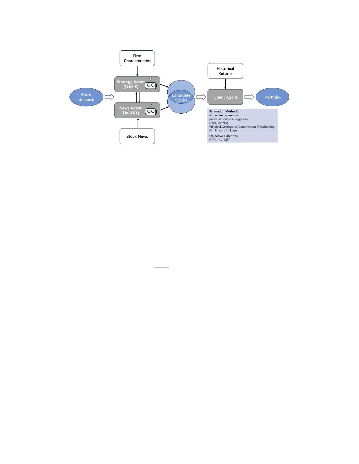
Designing Agen tic AI-Based Screening for P ortfolio In v estmen t Mehmet Caner ∗ A gostino Capponi † Na than Sun ‡ Jona than Y. T an § Marc h 25, 2026 Abstract W e introduce a new agen tic artiﬁcial in telligence (AI) platform for p ortfolio management. Our architecture consists of three la yers. First, t wo large language mo del (LLM) agents are assigned sp ecialized tasks: one agent screens for ﬁrms with desirable fundamentals, while a sen timent analysis agent screens for ﬁrms with desirable news. Second, these agen ts deliberate to generate and agree up on buy and sell signals from a large portfolio, substantially narro wing the p o ol of candidate assets. Finally , w e apply a high-dimensional precision matrix estimation pro cedure to determine optimal portfolio w eights. A deﬁning theoretical feature of our frame- w ork is that the num b er of assets in the portfolio is itself a random v ariable, realized through the screening pro cess. W e in tro duce the concept of sensible scr e ening and establish that, under mild screening errors, the squared Sharp e ratio of the screened portfolio consisten tly estimates its target. Empirically , our metho d ac hieves sup erior Sharp e ratios relativ e to an unscreened baseline portfolio and to conv entional screening approac hes, ev aluated on S&P 500 data ov er the p erio d 2020–2024. Keywor ds: P ortfolio screening, Agentic design, Sharpe-Ratio, precision matrix estimation. ∗ North Carolina State Universit y , Nelson Hall, Departmen t of Economics, NC 27695. Email: mcaner@ncsu.edu. † Colum bia Universit y . Departmen t of Industrial Engineering and Op erations Research and Colum bia Business Sc ho ol. Email: ac3827@colum bia.edu. ‡ Colum bia Univ ersity . Departmen t of Industrial Engineering and Op erations Research. Email: nathan.sun@colum bia.edu. § Colum bia Univ ersity . Departmen t of Industrial Engineering and Op erations Research. Email: jyt2123@colum bia.edu. 1 “We ne e d new AI mo dels for the r e al world—quantitative mo dels. . . AI for the quantita- tive world is something else entir ely, fo cusing on cr e ating novel me dic al t r e atments, de novo material scienc e, and advanc e d risk management and p ortfolio c onstruction .” — Jac k D. Hidary , CEO of Sandb ox AQ. The Wal l Str e et Journal , Opinion: “America Needs AI that can do Math,” F ebruary 17, 2026. “Ilya Sutskever has r e c ently b e en adding his voic e to the b eyond LLM c amp, stating that we won ’t r e ach artiﬁcial gener al intel ligenc e with lar ge language mo dels alone .” — Jac k D. Hidary , CEO of Sandb ox AQ. The Wal l Str e et Journal , Opinion: “America Needs AI that can do Math,” F ebruary 17, 2026. 1 In tro duction P ortfolio formation is a foundational concept in the ﬁnance literature. There are sev eral w ell- kno wn p ortfolio formations, including the global minim um v ariance p ortfolio, the Marko witz mean- v ariance p ortfolio, and the maxim um Sharp e ratio p ortfolio. T raditionally , these frameworks were dev elop ed and implemented b y h uman analysts throughout the t wen tieth cen tury . With the adv ent of large language mo dels coupled with deep learning-based estimation in the t wen t y-ﬁrst century , there are now artiﬁcial intelligence-driv en portfolios. V ery recently , m ulti-agent AI systems hav e b een applied to portfolio optimization. This pap er con tributes to this emerging literature by developing a high-dimensional portfolio management framew ork that in tegrates sto ck screening with p ortfolio optimization. Ev ery inv estmen t decision in volv es tw o distinct tasks: selecting which sto c ks to hold and determining their optimal weigh ts. Accordingly , b oth the set of selected sto cks and their p ortfolio weigh ts are treated as endogenous outputs of our framework. Rather than applying quan titative metho ds to the full sto ck univ erse or assigning equal weigh ts to an arbitrary subset, we propose an initial screening stage in which LLM- based agents generate buy and sell signals. A quantitativ e precision matrix estimation metho d then determines optimal inv estmen t weigh ts for the screened stocks. This tw o-stage approac h yields p ortfolios concen trated in stocks with strong return-generating p otential, ac hieving superior Sharp e ratios relative to standard b enchmarks. By incorp orating sto ck screening, the framew ork delib erately departs from index mimic king, aiming instead to generate excess returns, analogous to adopting a large trac king error relativ e to a b enchmark index in order to enhance risk-adjusted p erformance. A useful analogy is the selection pro cess of a sp orts team. After observing practice sessions, the manager chooses the b est play ers to form the starting lineup for game da y . The choice of the optimal subset of play ers can dramatically improv e team performance, and similarly , selecting the optimal subset of sto c ks may achiev e higher p erformance than using the en tire universe. Note that 2 b y setting up trac king error and weigh t constraints on p ortfolios, b oth industry practitioners and regulators mo ve a w ay from using all universe-indexing strategies. A recen t pap er by Caner and F an ( 2026 ) outlines how to form p ortfolios based on data-dep endent inequality constrain ts and establishes high-dimensional consistency of these p ortfolios. They demonstrate that the Sharp e ratio, returns, and collectiv e risk of a subset of stocks can do better than those of a b enchmark index. Because their restrictions are giv en b y m utual fund prospectuses and go vernmen t regulators, there is no p erformance-based screening inv olv ed in forming their p ortfolios. A study b y Arv anitis et al. ( 2024 ) presen ts strong economic and ﬁnancial theoretical foundations explaining wh y a sparse p ortfolio can perform b etter than or equal to the mark et index. Our m ulti-agent AI framew ork consists of three co ordinated la yers. In the ﬁrst la y er, t w o sp ecial- ized LLM agen ts op erate in parallel: an LLM-Strategy agen t (LLM-S), whic h screens stocks based on fundamental ﬁrm c haracteristics, including log ﬁrm size, bo ok-to-market ratio, and t w elve-mon th momen tum, and a FinBER T-based sen timent agen t, whic h analyzes ﬁnancial news articles to gen- erate monthly sen timent-driv en signals. These tw o agents op erate on complementary frequencies: LLM-S is retrained annually , capturing slow-mo ving structural narratives ab out ﬁrm quality , while FinBER T is up dated monthly to respond to fast-moving news sentimen t. In the second la yer, the t wo agents delib erate and reac h a consensus via an intersection-based decision rule, narro wing the candidate p o ol from the full S&P 500 to a high-con viction subset av eraging approximately 22 stocks. In the third lay er, a quantitativ e optimization algorithm applies state-of-the-art high-dimensional precision matrix estimation tec hniques, such as including no dewise regression ( Meinshausen and B ¨ uhlmann ( 2006 )), residual no dewise regression ( Caner et al. ( 2023 )), POET ( F an et al. ( 2013 )), deep learning-based metho ds, and nonlinear shrink age, to determine optimal p ortfolio w eigh ts un- der global minimum v ariance, mean-v ariance, and maximum Sharp e ratio ob jectives. The winning metho d-ob jectiv e com bination is selected based on out-of-sample Sharpe ratio p erformance. W e show that not every m ulti-agen t AI conﬁguration creates v alue, and that the design of the agen t team is critical. W e demonstrate this systematically by comparing our full multi-agen t system against a rich set of alternatives: purely quantitativ e strategies without any screening, single-agent LLM systems (LLM-S alone or FinBER T alone), conv en tional screening metho ds (logistic regres- sion, human analyst recommendations, and the Novy-Marx ( 2013 ) proﬁtabilit y-and-v alue screen), and h ybrid systems that incorp orate human analyst judgment alongside AI agen ts. In each case, our full Agen tic AI architecture, sp eciﬁcally tw o sp ecialized LLM screening agents plus a quantita- tiv e weigh ting metho d, dominates. W e sho w that incorp orating human analyst recommendations in to the AI ensemble consisten tly de gr ades p erformance, a ﬁnding w e attribute to the b ehavioral and emotional biases that human analysts inevitably carry in to their recommendations. This re- sult provides a concrete, quan titative answer to the practical criticism that the ﬁnancial v alue of AI-based systems is diﬃcult to measure. 1 1 “Early adopters who rushe d into AI pilots and even deployment last ye ar often hit a wal l and le arne d some har d lessons. . . Critic al ly, they found it was har d to me asur e ﬁnancial r eturns .” — Isab elle Bousquette, The Wal l Str e et Journal , Business Section, page B4: “AI soft w are pro ves to be tougher sell than b efore,” F ebruary 19, 2026. 3 Bey ond the empirical results, we make a nov el theoretical contribution to the high-dimensional p ortfolio literature. A deﬁning feature of our framew ork is that the n um b er of assets in the p ortfolio is not ﬁxed in adv ance, but is itself a random v ariable realized through the screening pro cess. The existing high-dimensional p ortfolio literature, including F an et al. ( 2011 ), Caner et al. ( 2023 ), and Caner and F an ( 2026 ), treats p ortfolio dimension as a deterministic, known sequence. W e depart from this con ven tion b y in tro ducing the concept of sensible scr e ening : a screening pro cess that, ev en when it makes mild errors in selecting the exact composition of the optimal p ortfolio, alwa ys includes the optimal sto cks when selecting enough assets and never selects purely sub optimal ones. Under sensible screening and standard precision matrix consistency conditions, we establish in Theorem A.1 that the squared Sharp e ratio of the screened p ortfolio consistently estimates its target, ev en when the screening pro cess is imperfect. Our em pirical analysis cov ers the S&P 500 from January 2020 to April 2024, a p erio d en- compassing noticeable even ts including the COVID-19 shock, the 2022 dra wdown, and the strong reco very of 2023. The S&P 500 index ac hieves an annualized Sharp e ratio of 0.6324 o ver this windo w. Under a purely quan titativ e strategy without screening, only one method-ob jective com- bination (nonlinear shrink age paired with the maximum Sharp e ratio ob jective) manages to b eat this b enchmark. By contrast, our multi-agen t AI framew ork b eats the mark et in all but one of the ﬁfteen metho d-ob jectiv e com binations we consider, with a p eak ann ualized Sharpe ratio of 1.1867, an 88% impro v ement ov er the index. W e extend the ev aluation to a nearly ten-year horizon span- ning January 2015 to April 2024, and ﬁnd that the Agen tic AI architecture contin ues to dominate, ac hieving a p eak Sharp e ratio of 0.9429, ab o ve the mark et b enchmark of 0.7298. These gains are accompanied by substan tially higher annu alized returns: the b est Agentic AI conﬁguration deliv ers a 36.34% annualized return ov er the ﬁve-y ear window, compared to 19.99% for the b est purely quan titative baseline. F or our quantitativ e strategy , w e follo w the established literature and form w eigh ts according to global minim um v ariance (GMV), Marko witz mean-v ariance (MV), and maximum Sharp e ratio (MSR) ob jectiv es. Our quan titative estimation metho d applies a matrix-based inv esting strategy , where estimation techniques form the ro ws and diﬀerent portfolio ob jectives form the columns. The winner within this matrix is the technique-ob jective combination that ac hiev es the highest Sharp e ratio for the out-of-sample time perio d b eing ev aluated. F or example, in T able 1 , the winner from Jan uary 2020 to April 2024 is the nonlinear shrink age metho d of Ledoit and W olf ( 2020 ) combined with the maximum Sharpe ratio portfolio. The rest of the pap er pro ceeds as follows. Section 2 provides bac kground on large language mo del and discusses our proposed Agen tic AI framework. Section 3 introduces the sto ck screen- ing framew ork, including the LLM-S and FinBER T agen ts, alternativ e screening b enchmarks, the algorithm, and our theoretical result on screened portfolio. Section 4 describes the quantitativ e high-dimensional portfolio weigh t formation metho ds. Section 5 presen ts our empirical results, in- cluding the main ﬁve-y ear ev aluation, robustness chec ks, and the extended ten-y ear analysis. W e 4 conclude in Section 6 . App endix A contains tec hnical pro ofs, Appendix B provides details on the precision matrix estimation techniques, and App endix C presen ts additional material including extended results, long-short strategies, LLM-S prompts and outputs, and No vy-Marx screening comparisons. 2 Agen tic AI P ortfolio Management F ramew ork W e pro vide bac kground on large language mo dels and their applications in ﬁnance. W e then describ e the architecture of our prop osed multi-agen t p ortfolio managemen t system and explain ho w it addresses the main metho dological concerns raised in the literature. 2.1 Large Language Mo dels Unlik e their predecessors, LLMs exhibit a human-lik e quality of text generation and deep con textual reasoning. These capabilities stem from the transformer arc hitecture ( V asw ani et al. , 2017 ), whic h lev erages self-attention mechanisms to capture long-range dep endencies in text far more eﬀectively than earlier recurrent or conv olutional approac hes. 2 LLMs are trained on massive datasets, optimizing a v ast n umber of parameters using deep learning estimators within a transformer structure, leading to signiﬁcant performance improv e- men ts across a range of tasks ( Bishop and Bishop , 2024 , pp. 390–391). Lev eraging self-sup ervised learning, LLMs acquire high-qualit y represen tations on unlab eled data and can then be further ﬁne- tuned to improv e performance. Fine-tuning is typically achiev ed through Lo w-Rank Adaptation (LoRA) or Reinforcement Learning from Human F eedbac k (RLHF). Alternative approaches include training the LLM from scratch on in-sample data to predict out-of-sample outcomes, or employing instruction ﬁne-tuning, where the mo del is trained on sp eciﬁcally generated prompt-resp onse pairs. Fine-tuned LLMs can substantially outp erform generic op en-source LLMs in sp ecialized domains suc h as sen timent analysis and ﬁnancial classiﬁcation ( Li et al. , 2024 , Section 4.1). An imp ortant practical consideration is the choice b et ween op en-source mo dels, suc h as LLaMA, and closed-source mo dels, suc h as GPT-4 or Claude. While op en-source mo dels oﬀer adv an tages in transparency , repro ducibility , and data control, Li et al. ( 2024 ) (Section 3) ﬁnd that closed-source mo dels curren tly achiev e sup erior p erformance on standard ﬁnancial b enchmarks, a gap that lik ely reﬂects diﬀerences in b oth mo del scale and the proprietary nature of their ﬁne-tuning pro cedures. 2 As documented in Kamath et al. ( 2024 ), models with fewer than ten billion parameters p erform near c hance lev el across a range of b enchmarks, including arithmetic reasoning, multilingual question answ ering, the 57-task Mas- siv e Multitask Language Understanding (MMLU) benchmark ( Hendrycks et al. , 2020 ), and semantic understanding ev aluations. Beyond this scale threshold, p erformance rises sharply , reaching appro ximately 30% on arithmetic tasks, 40–50% on m ultilingual question answering, and 60–70% on both MMLU and seman tic understanding b enchmarks. 5 2.2 LLMs in Finance: Related W ork LLMs oﬀer several adv antages for sto ck selection. Because their pre-trained nature enables robust zero-shot analysis, they eliminate the strict requiremen t for sup ervised learning. Rather than requiring costly and time-consuming mo del retraining, LLMs can rapidly execute simultaneous tasks suc h as sentimen t analysis and keyw ord extraction, and their ability to decomp ose complex tasks in to simpler sub-tasks makes them w ell suited to pro cessing the large v olumes of ﬁnancial rep orts in volv ed in stock selection ( Li et al. , 2024 ). A prominent empirical demonstration of this p otential is pro vided b y Chen et al. ( 2023 ), who show that integrating LLM-driven news analysis in to long- short p ortfolios can deliver v ery large Sharp e ratios o ver the 2004–2019 p erio d, outp erforming b oth the S&P 500 index and classical bag-of-w ords approac hes. The application of m ulti-agent systems to p ortfolio construction has b een considered by Zhao et al. ( 2025 ), who design a framework in which sp ecialized LLM agents collab oratively execute p ortfolio construction tasks. Their system comprises three agents, a fundamental equity agent, a sen timent agen t, and a v aluation agent, which must collab orativ ely discuss, ev aluate, and ﬁnalize decisions, thereby activ ely suppressing hallucinations made by an y single agent. This multi-agen t design mirrors the role of coordinated human analyst teams, whic h m ust synthesize ﬁnancial disclo- sures, earnings calls, ﬁnancial ratio analysis, market news, and research rep orts. Recent evidence b y Zhang et al. ( 2025 ) further supports this approac h: context-based LLMs outp erformed their base- line coun terparts by 8.6 percentage p oin ts on ﬁnancial reasoning tasks (T able 2 therein), suggesting that domain adaptation substantially improv es LLM p erformance. Despite this promise, Li et al. ( 2025 ) raise important metho dological concerns. Their cen tral argumen t is that existing studies demonstrating sup erior LLM performance often rely on v ery short ev aluation horizons (6–24 mon ths) and narrow asset universes (5 to 100 sto cks; see their T able 1). When ev aluated ov er extended horizons and across a larger cross-section of sto cks, they ﬁnd that LLM adv antages disapp ear, allowing simple b enchmarks such as buy-and-hold to dominate. They iden tify three sp eciﬁc sources of bias. First, lo ok-ahe ad bias , whereb y the mo del inadv ertently pro cesses future data during training or testing. Second, data sno oping , arising from rep eated testing on a static dataset leading to inﬂated results. Third, survivorship bias , whereb y delisted sto c ks are omitted, inﬂating apparen t returns. Evidence of lo ok-ahead bias is also documented b y Ludwig et al. ( 2025 ) and, in the sp eciﬁc con text of sto ck market predictions using ann ual US data o ver 2020–2023, b y Didisheim et al. ( 2025 ), who ﬁnd a small but detectable look-ahead bias at ann ual frequency and a substantially larger bias at high frequency . 2.3 Our Multi-Agen t P ortfolio Managemen t F ramew ork Our framework is a t wo-stage pipeline applied to the full S&P 500 univ erse. In the ﬁrst stage, an AI screening team, consisting of LLM-S and FinBER T op erating in concert, identiﬁes a targeted subset of sto c ks b y com bining fundamen tal analysis with sentimen t analysis of news articles. In the second stage, a quantitativ e precision matrix estimation algorithm assigns optimal p ortfolio 6 w eights to the screened sto c ks. This separation of screening and w eigh ting represents a scalable, end-to-end application of Agentic AI to p ortfolio construction, and is the primary architectural distinction from prior work suc h as Zhao et al. ( 2025 ), whose study ev aluates a randomly selected bask et of 15 tec hnology stocks rather than a comprehensiv e mark et-wide pip eline. W e tak e the follo wing steps to preven t lo ok-ahead bias. First, the dataset pro vided to the LLM-S agent contains no returns data, prev enting the agent from explicitly optimizing for future p erformance. Second, for each retraining date, the agent queries only ﬁrm characteristics strictly a v ailable on that date, so future characteristics cannot en ter the rule creation phase. Third, after the agent creates an in vestmen t rule, w e man ually apply it to S&P 500 ﬁrms to generate buy and sell recommendations, prev en ting an y dynamic adjustmen t the agent might otherwise mak e. F ourth, w e explicitly instruct the agent to use causal masking, which prev en ts the use of future test data during training. Fifth, as a robustness chec k, we verify that buy signals in each month do not systematically align with that month’s subsequen t returns. W e hav e not observed suc h alignment in our analysis. Note also that our FinBER T mo del’s w eigh ts w ere ﬁne-tuned on the Financial PhraseBank dataset ( Malo et al. , 2014 ), published in 2014, giving it a kno wledge cutoﬀ date prior to 2015. T o suppress hallucinations, w e deploy a consensus-based decision rule across agen ts. F or each sto c k, it is included in the ﬁnal recommendation only if b oth agen ts indep endently agree to buy or sell it; disagreement leads to exclusion. If the agen ts’ decisions are m utually exclusiv e across all stocks—prev en ting a null recommendation—we default to the union of their recommendations. With three agen ts, the rule b ecomes a t wo-out-of-three ma jority vote. A detailed description of the decision rule is pro vided in Section 5.2 . This intersection strategy reduces the hallucination risk inheren t in an y single agen t while preserving the complementarit y b etw een fundamen tal and sen timent signals. Sapkota et al. ( 2026 ) provide a systematic comparison of single-agent LLMs and m ulti-agent systems, do cumen ting that the deﬁning adv antage of multi-agen t architectures lies in dynamic task decomp osition, whereby a high-lev el ob jectiv e is broken do wn and distributed among sp ecialized agents. Our framework em b o dies this principle: LLM-S and FinBER T each address a distinct analytical sub-problem, and their outputs are combined through a formal consensus mec hanism rather than informal aggregation. F ollowing Li et al. ( 2025 ), we preven t data sno oping by using rolling windows rather than a ﬁxed in-sample training p erio d. W e address survivorship bias b y including all sto cks in the S&P 500, including those subsequently delisted. T o address the short-horizon critique of Li et al. ( 2025 ), we analyze t wo ev aluation perio ds. The ﬁrst spans ﬁve y ears and encompasses a diverse set of mark et regimes: the COVID-19 shock, the 2022 mark et drawdo wn, and the strong recov ery of 2023. The second extends the analysis to a nearly ten-y ear horizon from 2015 to 2024. 7 3 Sto c k Screening and W eigh ts Ha ving outlined the architecture of our multi-agen t system, we no w dev elop its core comp onen t in detail. W e formalize the concept of sto ck screening, describ e ho w our LLM agen ts implemen t it, present alternative screening b enc hmarks, and establish a theoretical result on the Sharp e ratio consistency of screened high-dimensional p ortfolios One argumen t for sto ck screening is the identiﬁcation of p otentially high-return assets within a large universe of sto cks. Additionally , sto c k screening can help preven t b ehavioral biases which are common among h uman analysts. The v alue of screening has been highligh ted in several studies, starting with the foundational work of F ama and F renc h ( 1992 ), who demonstrate that screening for small-cap and lo w price-to-b o ok sto cks leads to higher returns in the t w entieth cen tury . Je- gadeesh and Titman ( 1993 ) v alidate the idea of “price-p erformance” screening and consider the “momen tum” eﬀect, sho wing that sto cks p erforming well ov er the past 3-12 months tend to con- tin ue performing w ell in the near future. Piotroski ( 2000 ) introduces F-scores: nine accoun ting ratios to ﬁnd high quality sto c ks. Novy-Marx ( 2013 ) adds a quality-gross proﬁtabilit y criterion for v alue sto cks. In sum, screening generates higher returns and/or higher Sharp e Ratio p ortfolios for several reasons. First, due to the limited cognitiv e capacity of h uman beings, tec hnical analysis may b e more eﬀectiv e on a subset of sto c ks compared to, for example, a larger univ erse of a thousand sto c ks. Second, since inv estors are susceptible to narrativ e bias, ov erw eighting comp elling stories attac hed to assets rather than their fundamen tals ( Tversky and Kahneman , 1974 , 1983 ), a sys- tematic, quan titative screening approac h can help ident ify and exclude sto cks driv en primarily by sen timent rather than in trinsic v alue. F urther, ﬁnancially distressed ﬁrms can b e systematically identiﬁed by analyzing debt and liquidit y ratios and av oiding buying underp erforming or close to bankruptcy ﬁrms by using the Altman Z score (see Altman ( 1968 )). Eliminating or shorting distressed ﬁrms from the p ortfolio is another a v enue to higher returns. 3.1 LLM-S and FinBER T Our distinguishing approac h compared to the rest of the literature is that we pro vide a multi-agen t AI system that can screen stocks across a broader univ erse. W e start with developing our o wn LLM agen t, tailored at analyzing ﬁrm fundamental data. W e call this agen t LLM-S, abbreviated for LLM-strategy . Using standard AI agen t construction tec hniques, LLM-S pro duces a fundamen tals-based scoring rule to screen stocks. The ob jectiv e is to ﬁlter out ﬁrms that ha ve undesirable fundamentals, leaving b ehind only high-qualit y sto cks in the p ortfolio. W e utilize LLMs in a no v el w ay: w e prompt the LLM to adopt the p ersona of a p ortfolio manager, and w e ultimately let the LLM decide upon a sp eciﬁc buy and sell strategy based on fundamen tals data. In doing so, w e also gain insight into its explanation on why it has 8 c hosen a sp eciﬁc buy and sell strategy . At the end of this c hoice, LLM-S is ask ed to justify its screening c hoice. W e next describ e the main steps of our LLM-S agen t. First, LLM-S uses three factors to initiate the algorithm: log ﬁrm size (mv e), b o ok-to-market ratio (bm), and 12-mon th momentum (mom12m). W e select these sp eciﬁc factors because they represent the most robust and widely accepted predictors of cross-sectional stock returns in the empirical ﬁnance literature, capturing the size of the ﬁrm, its v aluation, and its recent performance, resp ectively (see F ama and F rench ( 1992 ) and Carhart ( 1997 )). F urthermore, our preliminary testing rev ealed that using this parsimonious set of factors is crucial for the LLM. Expanding the factor set to include the F ama-F rench 5-factor v ariables plus momentum empirically degraded the mo del’s performance. So it is critical to model the right LLM agent rather than simple use of LLM. This is very muc h related to architecture of LLM agents and the aim here is to ﬁnd agents that add economic or ﬁnancial v alue to the ﬁrm. This design of the architecture is crucial to reﬂect criticism in the practical ﬁnancial world ab out the v alue of LLM (see F o otnote 1 in Introduction). The LLM-S is instructed to follo w the following four steps on its o wn without sup ervision, and w e explicitly instruct it to use causal masking to prev ent lo ok-ahead bias. 1. Explore the data to understand extreme v alues in factors, clustering or breakp oints, and correlations betw een factors. 2. Dev elop clear rules based on economic in tuition. 3. Deﬁne speciﬁc thresholds for buy and sell. 4. Pro vide rationale for decisions. Eac h of these points is extensively detailed in App endix C , where a snipp et of our co de is also sho wn. These ab ov e four rules can b e thought of the following pipeline: data analysis, developing rules for buying and selling, deciding on exact thresholds, and ﬁnally , an explanation of its decision rationale. By using size, b o ok-to-market, and momentum as features, our LLM-S ﬁlters the univ erse of stocks to retain only those exhibiting c haracteristics historically asso ciated with risk premia. The strategy also inheren tly acts as a signal enhancer: by isolating ﬁrms with the most extreme signals, LLM-S constructs a subset of ﬁrms with high factor exp osure. This provides the quantitativ e estimation method a highly informativ e candidate po ol to optimize upon. Our LLM-S deviates from traditional screening metho ds in a few fundamen tal wa ys. Firstly , traditional metho ds often rely on ﬁxed heuristic rules that are static o ver time (see, for example, Piotroski ( 2000 ) and Mohanram ( 2005 )). In con trast, our LLM-S is rerun once every y ear to ensure the most recen t rules, and it has the ability to choose exact thresholds (i.e. it has the abilit y to con textualize the rule based on the distribution of the data for a sp eciﬁc date). While previous metho ds mostly rely on backw ard-lo oking training to determine scoring rules (see, for example, 9 Altman ( 1968 ) and Asness et al. ( 2019 )), we lev erage the broad knowledge em b edded in pre- trained modern LLMs. Because these models hav e already learned extensive ﬁnancial principles from a massiv e set of data, we can use a “zero-shot” approach. That is, the mo del generates the scoring rule directly from its in ternal kno wledge without requiring an y training. Lastly , the LLM provides the scoring rule plus the economic intuition b ehind it, pro viding a greater lev el of in terpretability . As an example, our LLM-S provided the following strategy and rationale for buy and sell decisions in year 2024 (more details regarding reasoning of this c hoice are in Appendix C ). - BUY Rule: This rule targets underv alued (high bm), reasonably sized ( mv e > 0 . 3) companies with p ositive momentum ( mom 12 m > − 0 . 5). 3 The economic in tuition is to buy companies that are curren tly c heap but ha v e shown some signs of recov ery or positive market sentimen t. - SELL Rule: This rule aims to sell companies that are ov erv alued (lo w bm), hav e negativ e momen tum ( mom 12 m < − 0 . 55), or are small in size ( mv e < − 0 . 75). Note that buy and sell rules underscore the presence of interaction eﬀects within ﬁnancial mark ets, aligning with the theoretical framework established in Section 3.6 of Kelly and Xiu ( 2023 ). In our example ab o ve, our buy decision is reminiscent of the interaction term b etw een high b o ok-to- mark et, reasonably sized, and positive momentum ﬁrms. Our sell decision can be similarly view ed as an interaction term. In sum, our buy and sell decisions are seen as analyzing the buy and sell decisions from a nonlinear framew ork in volving interaction b etw een factors. Our results can also b e related to an information theoretic approac h b y Hong et al. ( 2000 ), who demonstrates that the momen tum eﬀect in teracts with size of the ﬁrm and analyst cov erage. After in tro ducing LLM-S, to handle h uman biases and account for short-term news, we utilize FinBER T, a natural language pro cessing mo del sp ecialized in analyzing ﬁnancial text, to conduct sen timent analysis on recent stock news. FinBER T agent also makes buy-sell decisions. After discussing their buy and sell decisions, t w o agen ts decide on a consensus of buy-sell decisions. Once these LLMs decide which sto cks to buy and sell, we feed the screened sto cks in to quan ti- tativ e high-dimensional weigh t formation techniques (see Callot et al. ( 2021 ), Caner et al. ( 2023 ) using no dewise or residual no dewise regression resp ectively). These metho ds will b e describ ed in detail in subsequen t sections. In short, we combine LLM- and sen timent analysis-based screening with state-of-the-art high dimensional quan titative p ortfolio formation tec hniques. W e also connect our screening idea econometrically to high-dimensional p ortfolio analysis. The screening pro cess can b e conceptualized not just as selecting sto cks that can provide higher returns or Sharp e ratios, but it can also b e viewed as choosing the correct n umber of sto c ks among a large univ erse of them. Clearly , this screening c hoice is a random v ariable and aﬀects ho w w e c ho ose the weigh ts in our p ortfolio. First, let us denote the n um b er of sto cks chosen b y the screening pro cess as the random v ariable ˆ p . Also, denote by p ∗ the target (optimal) n umber of stocks, which is non-random, and p ≥ p ∗ ≥ 1, where p is the size of the en tire univ erse of sto c ks. It is worth 3 Note the m ve, bm, and mom12m features are standardized to ha ve mean 0 and v ariance 1. 10 emphasizing that, together with the num b er of sto cks, we hav e the sto cks themselves; for example, the optimal c hoice ma y b e Nvidia and P alan tir; hence giving us p ∗ = 2. W e ha ve the following deﬁnition of the screening pro cess. Let U represent the total univ erse of stocks. Deﬁnition: Sensible Screening. Let S ∗ ⊆ U denote the optimal p ortfolio, with |S ∗ | = p ∗ , and let ˆ S ⊆ U denote the set of sto cks selected b y the screening pro cess, with | ˆ S | = ˆ p . A screening pro cess is sensible if: (i) when ˆ p ≥ p ∗ , the optimal set is reco vered within the screened set: S ∗ ⊆ ˆ S ; (ii) when ˆ p < p ∗ , the screened set is en tirely comp osed of optimal sto cks: ˆ S ⊂ S ∗ . A sensible screening pro cess never selects a sto ck that do es not b elong to the optimal p ortfolio, and alwa ys includes the optimal p ortfolio when it selects enough sto cks. F or example, supp ose p ∗ = 2 and the optimal p ortfolio is S ∗ = { Nvidia, P alan tir } . If ˆ p = 3, sensible screening requires that ˆ S = { Nvidia, P alantir, X } for some third sto ck X / ∈ S ∗ , i.e., the tw o optimal sto cks are alwa ys included. If instead ˆ p = 1, sensible screening requires that the single selected stock be either Nvidia or P alan tir. The main idea of our theoretical analysis is to treat the num ber of sto c ks in the p ortfolio as a random v ariable, one that is realized through the screening pro cess b efore any weigh ts are estimated. Under sensible screening, and robust to mild screening errors, we sho w that the Sharp e ratio of the screened p ortfolio consisten tly estimates the target Sharp e ratio of the optimal stock universe. This result app ears to b e new in the high-dimensional p ortfolio literature, where the comp osition of the in vestable set is typically tak en as giv en. W e next turn to the screening pro cedures used in our empirical analysis. 3.2 Diﬀeren t Screening Metho ds As a b enchmark, we also consider alternativ e screening methods. W e consider sto c k picking b y h uman analysts, and a logistical regression-based stock picking metho d. In the ﬁrst method, w e use the buy/sell decisions of human analysts from IBES (Institutional Brokers Estimates System, accessed via WRDS) recommendations, and in the second one, w e use logistic regression to generate buy/sell signals as prop osed b y Chen et al. ( 2023 ) . The former also represen ts conv en tional human judgmen t, and the latter is a simple quan titativ e strategy for sto ck picking. Our b enc hmarking strategy is designed to disen tangle three sources of p otential p erformance gains: sto ck screening p er se, the use of LLMs for screening, and the b eneﬁts of a m ulti-agent arc hitecture. T o this end, we compare our m ulti-agent system against four classes of alternativ es. First, w e b enchmark against conv en tional screening methods, namely momentum and v alue screens, to assess whether an y p erformance improv ement stems from screening itself rather than from the speciﬁc screening tec hnology . Second, we compare against single-agen t LLM screeners, suc h as LLM-S alone or FinBER T com bined with the quantitativ e method, to isolate the contribution of the multi-agen t 11 arc hitecture. Third, we consider alternative m ulti-agent conﬁgurations, including hybrid systems that com bine LLM-S, FinBER T, and h uman judgment screening, with portfolio decisions delegated to a quan titativ e optimization metho d. Finally , we compare against the quan titativ e-metho d-only baseline, whic h abstracts from screening en tirely , to quan tify the marginal v alue of LLM-based sto c k selection 3.3 Algorithm Our algorithm screens p sto cks and subsequen tly feeds the results to a quantitativ e precision matrix estimation method, who determines the p ortfolio weigh ts. Our approac h proceeds as follo ws: 1. The LLM-S agen t and the FinBER T agen t indep enden tly decide whic h sto cks to buy/sell. W e rerun the LLM-S agent each y ear, and the FinBER T agent eac h month. W e do this to capture the slo w-mo ving economic narrative that the LLM-S aims to capture while also preserving the fast-moving news that FinBER T captures. This mirrors classical p ortfolio literature (see F ama and F rench ( 1992 )) and mo dern ML approaches (see Gu et al. ( 2020 )) that reﬁt computationally heavy mo dels annually . 2. According to their decision rule (which will b e discussed in Subsection 5.2 ), the mo dels reach a consensus, if applicable, on a subset of ˆ p sto cks to buy/sell, where 1 ≤ ˆ p ≤ p . 3. These ˆ p sto cks are pro vided to the quan titative metho d, whic h computes optimal portfolio w eights based on a strategy described in Section 4 . These dep end on a com bination of a metho d and ob jective. 4. Repeat for all months. W e use the ann ualized out-of-sample Sharpe ratios as the primary measure of p erformance. W e illustrate the algorithm in Figure 1 . Denote the cov ariance matrix of outcomes as Σ. As an illustration of the third step, consider the case where the p ortfolio ob jectiv e is global minimum v ariance (GMV) and the precision matrix, whic h is the inv erse of the co v ariance matrix of outcomes, Γ : = Σ − 1 is estimated via no dewise regression. The GMV weigh ts, computed via the no dewise-GMV metho d, are then given by ˆ w = ˆ Γ1 ˆ p 1 ′ ˆ p ˆ Γ ˆ p 1 ˆ p , where ˆ Γ is the ˆ p × ˆ p estimated precision matrix of the screened sto c ks and 1 ˆ p ∈ R ˆ p is a vector of ones. More details are describ ed in Section 4 . Note the fact that dimension of the precision matrix ( ˆ p ) is a random v ariable, determined by the screening pro cess prior to estimation. This stands in con trast to the existing high-dimensional p ortfolio literature, where the num b er of assets is treated 12 Figure 1: An illustration of the algorithm. LLM-S and FinBER T ﬁrst screen for candidate sto cks to in v est in, and the precision matrix estimation tec hnique assigns w eigh ts to these stocks. as a deterministic sequence growing at a kno wn rate; see, e.g., F an et al. ( 2011 ), Ledoit and W olf ( 2017 ), Caner et al. ( 2023 ), and Caner and F an ( 2026 ). 3.4 Screened P ortfolio based Sharp e Ratio Analysis Let c S R ˆ p denote the Sharpe ratio estimator based on the screened p ortfolio of dimension ˆ p , and let S R p ∗ denote the target Sharp e ratio of the optimally screened p ortfolio. In Theorem A.1, w e establish that under sensible screening with mild errors (formalized in Assumption A.1),       c S R 2 ˆ p S R 2 p ∗ − 1       = o p (1) . That is, the squared Sharpe ratio of the screened GMV p ortfolio consisten tly estimates its target, ev en when the screening pro cess is imp erfect. T o our kno wledge, this is the ﬁrst such result in the high-dimensional p ortfolio literature, where p ortfolio dimension is typically treated as ﬁxed and kno wn. The result holds for an y sensible screening pro cess satisfying Assumption A.1, and is therefore compatible with a broad class of precision matrix estimators, including those of F an et al. ( 2011 ) and Caner et al. ( 2023 ). The results will hold true in large p ortfolios as long as the precision matrix estimation of asset returns are consisten t. Case-b y-case analysis can b e obtained under w eak er conditions than the general level assumptions in App endix A . 4 Quan titativ e Based High Dimensional Portfolio W eigh t F orma- tion One of the main empirical discov eries by Caner and F an ( 2025 ) and Caner et al. ( 2023 ) is a joint analysis of precision matrix estimation techniques with ob jectiv e functions. The main insigh t will 13 b e in v esting in the winner of the b est com bination of precision matrix estimation technique and ob jectiv e function. In all the quantitativ e-based techniques, we let the num b er of assets to be p , and time series to b e n . W e index assets by j = 1 , · · · , p and index time by t = 1 , · · · , n . 4.1 Precision matrix estimation In this section, we discuss methods for high dimensional p ortfolio selection. W e include brief descriptions of ﬁve diﬀerent metho dologies for precision matrix estimation, representing a v ariet y of approaches ranging from statistical shrink age to factor mo dels to ML-based regression techniques. These metho ds address the challenge of estimating the precision matrix Γ = Σ − 1 when the num ber of assets exceeds the sample size. W e use the estimated ˆ Γ of these metho ds as the precision matrix when making portfolio decisions in future sections. In eac h of the metho ds b elo w in Section 4 , w e use a constant p assets to determine the estimator for the precision matrix. In the appendix, w e show ho w a screened univ erse of stocks c hange the precision matrix estimation. A rigorous, in-depth description of each metho d can b e found in App endix B . 4.1.1 No dewise regression In tro duced b y Meinshausen and B ¨ uhlmann ( 2006 ) and applied to portfolio risk-estimation by Cal- lot et al. ( 2021 ), no dewise regression estimates the precision matrix directly via p Lasso linear regressions. By mo deling eac h asset’s excess return as a linear combination of all other as sets’ excess returns (i.e. y t,j = y ′ t, − j γ j + η t,j ), this metho d explicitly imp oses sparsit y on the ro ws of the precision matrix. T o accoun t for high dimensions, the coeﬃcients are estimated via a Lasso regression: ˆ γ j = argmin γ " || y j − Y − j γ || 2 2 n + 2 λ j || γ || 1 # , where y j is the n × 1 vector of returns for asset j , Y − j is the n × ( p − 1) matrix of returns for all other assets, and || · || 1 and || · || 2 denote the standard l 1 and l 2 norms. High-dimensional consistency is ac hieved by optimizing the p enalty parameter λ j via a Generalized Information Criterion (GIC). The precision matrix can b e constructed directly by using matrix algebra and deﬁning the diagonal elemen ts ˆ Γ j,j = ˆ τ − 2 j and the vector of oﬀ-diagonal elements for j − th row ˆ Γ j, − j = − ˆ τ − 2 j ˆ γ ′ j , where ˆ τ 2 j = || y j − Y − j ˆ γ j || 2 2 n + λ j || ˆ γ j || 1 . W e form eac h row j of ˆ Γ by using the main diagonal term ˆ Γ j,j and the oﬀ-diagonal term in row j as ˆ Γ j, − j . Then stac king each row one up on other we form ˆ Γ. ˆ Γ is then the no dewise estimator of the precision matrix. 4.1.2 Residual no dewise regression Prop osed b y Caner et al. ( 2023 ), this approac h extends standard no dewise regression b y in tegrating factor models. The asset returns are modeled b y y t,j = b ′ j f t + u t,j , where f t represen ts a K × 1 v ector of observ able factors (e.g., the F ama-F rench three-factor mo del) and b j : K × 1 represents 14 the factor loadings. Unlik e standard no dewise regression, whic h assumes the precision matrix of returns is sparse, this metho d only assumes sparsity in the precision matrix of the unobserved idiosyncratic errors, Σ − 1 u . After the observ able factor structures are remov ed via ordinary least squares, no dewise regression is applied to the residuals to estimate ˆ Ω ≈ Σ − 1 u . The ﬁnal precision matrix of returns is reconstructed analytically using the Sherman-Morrison-W o o dbury formula: ˆ Γ = ˆ Ω − ˆ Ω ˆ B [ ˆ Σ − 1 f + ˆ B ′ ˆ Ω sy m ˆ B ] − 1 ˆ B ′ ˆ Ω , where ˆ B is the p × K matrix of estimated factor loadings, ˆ Σ f is the sample cov ariance of the factors, and ˆ Ω sy m = ( ˆ Ω + ˆ Ω ′ ) / 2 is the symmetrized residual precision matrix estimate. 4.1.3 Principal Orthogonal Complemen t Thresholding (POET) Dev elop ed b y F an et al. ( 2013 ), POET is designed for linear factor mo dels ( y t,j = b ′ j f t + u t,j ) where the K common factors f t are unobserv able and must b e estimated. POET ﬁrst uses principal comp onen ts analysis (PCA) to estimate the unobserv able factors, then uses a thresholding metho d to estimate the co v ariance matrix of errors. Under the assumption that the cov ariance matrix of the remaining idiosyncratic errors (Σ u ) is sparse, POET applies a soft-thresholding technique to the error co v ariance matrix to eliminate spurious correlations, yielding ˆ Σ u,T h (w e leav e tec hnical details in Appendix B ). The ﬁnal precision matrix is reconstructed from the thresholded error cov ariance and the estimated factor structure: ˆ Γ = ˆ Σ − 1 u,T h − ˆ Σ − 1 u,T h ˆ B ( I K + ˆ B ′ ˆ Σ − 1 u,T h ˆ B ) − 1 ˆ B ′ ˆ Σ − 1 u,T h , where ˆ B is the matrix of PCA-estimated factor loadings and I K is the K × K iden tity matrix. 4.1.4 Deep learning T o capture complex, non-linear relationships b etw een asset returns and observ able factors, Caner and Daniele ( 2025 ) introduce a deep learning-based estimator. The asset returns are mo deled b y a m ulti-lay er neural net work, y t,j = g j ( f t )+ u t,j , where f t is a K -dimensional observ able column vector and g j ( · ) is an unknown function. This eﬀectiv ely decomp oses the total cov ariance matrix into a non-linear function co v ariance component and an idiosyncratic error co v ariance comp onent (Σ y = Σ g + Σ u ). Similar to POET, a targeted thresholding mechanism is applied to the error cov ariance matrix ( ˆ Σ u,T h ) to ensure stability . The ﬁnal precision matrix is then recov ered algebraically: ˆ Γ = ˆ Σ − 1 u,T h − ˆ Σ − 1 u,T h ˆ Σ g ( I K + ˆ Σ − 1 u,T h ˆ Σ g ) − 1 ˆ Σ − 1 u,T h , where ˆ Σ g is the estimated cov ariance matrix of the neural net work predictions. 15 4.1.5 Nonlinear Shrink age (NLS) In tro duced by Ledoit and W olf ( 2017 ) and adv anced by Ledoit and W olf ( 2020 ), Nonlinear Shrink- age (NLS) addresses the instability of the sample cov ariance matrix in high dimensions through mo difying its eigen v alues. Starting with the sp ectral decomposition of the sample co v ariance matrix S = U Λ U ′ (where U is the orthogonal matrix of eigenv ectors and Λ is the diagonal matrix of sample eigen v alues), NLS systematically mo diﬁes the sample eigenv alues while preserving the eigenv ectors. Utilizing the Hilbert transform of the sample sp ectral density (elab orated in App endix B ), NLS deriv es an optimal, closed-form ﬁnal estimator, whic h tak es on the form: ˆ Σ = U ˆ ∆ ∗ U ′ , where ˆ ∆ ∗ is the diagonal matrix of optimally shrunk eigen v alues. Conceptually , this lo cal shrink- age pulls disp ersed sample eigenv alues tow ard each other, correcting the s ystemic o ver-dispersion inheren t in high-dimensional settings and pro ducing a well-conditioned precision matrix estimator. W e then set ˆ Γ = ˆ Σ − 1 . 4.2 Ob jectiv e functions W e introduce three ob jectiv e functions that are heavily used in practice and provide the optimal w eight of the portfolios attac hed to these functions. These are the global minimum v ariance p ortfo- lio (GMV), the Marko witz mean-v ariance p ortfolio (MV), and the maximum Sharp e ratio p ortfolio (MSR). The GMV weigh ts are giv en b y w ∗ : = argmin w ∈ R p w ′ Σ w , such that w ′ 1 p = 1 . The solution to the ab ov e is w ell-known and is giv en by w ∗ = Γ1 p 1 ′ p Γ1 p . The GMV p ortfolio is designed to be v ery risk adverse, as it is designed to minimize the v ariance of a p ortfolio. It ma y b e a go o d device to provide a small return without to o muc h risk. A diﬀeren t ob jectiv e function that incorporates both return and v ariance w ould be the mean v ariance portfolio, whose w eigh ts are giv en b y w ∗ : = argmin w ∈ R p w ′ Σ w , such that w ′ 1 p = 1 , w ′ µ = ρ. Here, ρ is the target monthly return (in our empirics w e use ρ = 0 . 01). The mean return µ is estimated by the a verage return in our train window. The solution is also w ell-known and is given 16 b y w ∗ =  D − ρF AD − F 2  Γ1 p +  ρA − F AD − F 2  Γ µ, where A : = 1 ′ p Γ1 p , F : = 1 ′ p Γ µ , and D : = µ ′ Γ µ . Finally , the maximum Sharpe ratio portfolio is heavily used in practice, whose weigh ts are giv en b y w ∗ : = argmax w ∈ R p w ′ µ √ w ′ Σ w , such that 1 ′ p w = 1 . The solution is given by w ∗ = Γ µ 1 ′ p Γ µ . 5 Empirical Results This section addresses tw o empirical questions. First, do es combining LLM-based screening with a quan titative w eigh ting metho d pro duce sup erior out-of-sample Sharp e ratios relative to the quan- titativ e metho d op erating without any screening? This isolates the incremental v alue of the m ulti- agen t screening stage. Second, do con ven tional screening approac hes, speciﬁcally logistic regression- based screening and human analyst recommendations, achiev e comparable p erformance when paired with the same quan titative metho d? W e sho w that the m ulti-agent AI framework outp erforms both alternativ es across all speciﬁcations. W e also conduct a series of robustness chec ks. First, we ev aluate a hybrid agen t system (sp ecif- ically , FinBER T, LLM-S, plus h uman analyst recommendations) with the quantitativ e metho d to determine if incorp orating human judgmen t enhances or detracts from the Agentic AI system. Second, we assess whether a single-agent screening approach (pure FinBER T or LLM-S) and the quan titative metho d will outp erform the tw o LLM agents together plus the quantitativ e metho d. Lastly , we ev aluate how human-only screening with the quan titative metho d p erforms compared with only the quantitativ e metho d. This provides a measurable assessment of the v alue of tradi- tional h uman screening. W e rep ort the follo wing p erformance measures: the mean (out-of-sample) monthly return, the out-of-sample v ariance, and the out-of-sample Sharp e ratio. All of these will b e calculated with a transaction cost of 10 basis p oints. Let y P,t +1 = ˆ w ′ t y t +1 b e the gross return of the p ortfolio at time t + 1, and ˆ w t b e the weigh ts of the p ortfolio at time t with some metho d. Then the net returns are giv en b y y net P,t +1 = y P,t +1 − c (1 + y P,t +1 ) p X j =1 | ˆ w t +1 ,j − ˆ w t,j 1 + y t +1 ,j 1 + y P,t +1 | , where c is the transaction cost. 17 Then the out-of-sample mean return is deﬁned as µ net = 1 T − T I T − 1 X t = T I y net P,t +1 . Note that µ net is the a verage out-of-sample p ortfolio return ov er rolling windows, rep orted as “Returns” in our tables. The out-of-sample v ariance is deﬁned as ˆ σ 2 net = 1 T − T I − 1 T − 1 X t = T I ( y net P,t +1 − µ net ) 2 , and reported as “V ariance” in our tables. Lastly , the out-of-sample Sharpe ratio is deﬁned as S R net = µ net ˆ σ net . 5.1 Data Our mon thly fundamentals dataset co v ers all S&P 500 constituents from Jan uary 2005 to April 2024, sourced from CRSP and Compustat, and includes three ﬁrm characteristics: size, b o ok-to- mark et ratio, and 12-month momentum. This dataset is a subset of Green et al. ( 2017 ), and the sample ends in April 2024 to align with the co verage of our news dataset. F ollowing Green et al. ( 2017 ), we winsorize all c haracteristics at the 1st and 99th percentiles, standardize each to zero mean and unit standard deviation, and replace missing v alues with zero, implying that ﬁrms with missing data are assigned the cross-sectional a v erage c haracteristic for that mon th. 4 F or eac h mon th t ’s return, w e calculate their features at the end of mon th t − 1. W e assume that ann ual accoun ting data are av ailable at this time if the ﬁrm’s ﬁscal year ended at least six mon ths b efore t − 1. 5.2 Metho d 5.2.1 Stage 1: Screening Agen ts The ﬁrst stage to our mo del consists of a screening agen t. As describ ed ab ov e, this can b e a con ven tional screening agen t, such as human analysts, but we also consider LLMs as screening agen ts. The tw o suc h agents are LLM-S, a fundamen tals-based LLM that generates buy , sell, and hold signals according to mon thly ﬁrm fundamen tals data, and FinBER T, a news-based agent that generates signals based on sen timent analysis on news eac h mon th. 4 Similar imputation metho ds for missing data are the standard in empirical asset pricing: used in Gu et al. ( 2020 ), Kozak et al. ( 2020 ), and Kelly et al. ( 2025 ). Chen and McCo y ( 2024 ) speciﬁcally recommend using mean imputation for ML studies. See fo otnote 5 in Green et al. ( 2017 ) for additional justiﬁcation. 18 W e ﬁrst describ e the con v entional screening approaches. The approac h using human analysts is based on analyst recommendations on the IBES dataset. Since analyst recommendations ma y b ecome stale quic kly , we use an exp onen tially-decreasing w eight on each analyst’s recommendation, based on ho w far their date of recommendation is to month-end (we use a half-life of 7 da ys). W e then tak e the weigh ted sum of all analysts’ recommendation for e ac h S&P500 stock, and calculate the c hange in the weigh ted sum mon th-to-month. If the c hange in recommendations is greater than 0 . 5 (resp ectively , less than − 0 . 5), we interpret that as a sell (resp ectively , buy) signal. All others are hold signals. The approach using logistic regression runs a simple logistic regression cross-sectionally for all ﬁrms in a speciﬁc date. W e then ev aluate the out-of-sample probabilities for the next month, assign buy signals to ﬁrms with probabilities in the top decile, and assign sell signals to ﬁrms with probabilities in the b ottom decile. Ev erything else is assigned a hold signal. No w we describ e the LLM screening approaches. FinBER T is a s p ecialized, pre-trained natural language pro cessing mo del designed for ﬁnancial sentimen t analysis (see Araci ( 2019 )). W e use S&P 500 news articles provided online at Hugging F ace. 5 F or each sto c k-mon th combination, w e use FinBER T to analyze all news articles in that month. W e deﬁne a ﬁrm’s sen timen t score to be the p ositive FinBER T probabilit y minus the negative FinBER T probabilit y and using the same exponentially-decreasing weigh ted sum as ab ov e to accoun t for potentially stale news. If the sen timent score is greater than 0 . 1 (respectively less than − 0 . 1), w e assign a buy signal (respectively assign a sell signal). All other stocks are assigned hold signals. Lastly , w e describ e LLM-S. W e use Gemini 2.0 Flash in CrewAI and give it the necessary to ols to access ﬁrm fundamentals data in a giv en date. It then considers the distribution of ﬁrm size, b o ok-to-mark et, and momentum v alues for that date, and outputs a deterministic scoring rule for buys, holds, and sell signals. T o leverage the zero-shot capabilities of LLMs, w e only provide ﬁrm c haracteristics to the LLM at the end of the y ear, and ask it to provide buy , hold, and sell signals for the next y ear. Imp ortantly , the agen t does not use statistical learning on historical data. Instead, it relies on pretrained domain kno wledge and in-con text reasoning to analyze the curren t cross-section of ﬁrms and pro duce screening decisions. Lastly , to ensure a sanity chec k, we also ask the agen t to pro vide its economic in tuition for why it chooses the scoring rule that it do es. W e ha ve included snapshots of our prompts and an example output in the appendix. T o accoun t for any p otential lo ok-ahead biases, w e explicitly instruct the agen t to use causal masking in the prompt. In the following sections, we also consider ensembles of agents (for example, LLM-S + Fin- BER T), geared at reducing hallucinations/inaccurate recommendations for eac h agent. The deci- sion rule for the ensemble is given as follo ws: given an ensem ble of agen ts A 1 and A 2 , who pro vide sets of buys and sells S 1 and S 2 , resp ectively , the ensem ble A 1 + A 2 recommends the set S 1 ∩ S 2 to inv est in. How ever, if the cardinality of the intersection is less than or equal to one sto c k: | S 1 ∩ S 2 | ≤ 1, then it recommends the set S 1 ∪ S 2 . This is saying that ideally , we would lik e to take 5 https://huggingface.co/datasets/KrossKinetic/SP500- Financial- News- Articles- Time- Series 19 the ﬁrms in the consensus of both agen ts. How ev er, if the t wo agents cannot reac h a consensus, w e tak e all of their recommendations. If w e ha v e an ensemble of three agen ts A 1 , A 2 , and A 3 , with recommendations S 1 , S 2 , and S 3 , resp ectiv ely , then the ensemble A 1 + A 2 + A 3 will recommend sto c ks that b elong in at least tw o distinct sets. This is akin to taking the ma jorit y vote b etw een three agen ts. The ab ov e particular decision rule defaults to the union of sets in case the in tersection is trivial. In our analysis in Section 5.3 , our b est model, FinBER T+LLM-S, has trivial in tersections 50% of all dates - hence w e default to the union to a v oid a mostly empty p ortfolio. Other wa ys of defaulting, suc h as choosing the highest SR single agen t (FinBER T) when the in tersection is empty , leads to empirically worse p erformance. W e stress that the ma jorit y of the p erformance is due to the in tersection rather than the union. F or example, in the FinBER T+LLM-S with MV ob jectiv e and deep learning, 1 . 037 out of the 1 . 187 Sharpe ratio is due to the in tersection, with the union only ha ving a Sharp e ratio of 0 . 545. This matches with our intuition, as the in tersection is meant to wards reducing hallucinations and inaccurate recommendations b etw een the tw o agen ts. W e explain our c hoice of decision rule further. T o prev ent a hallucination of o verselecting stocks and not screening well, we use the intersection rule for t wo agent system. If their in tersection is empt y , then it is clear that there is no ov erselection due to hallucination, and it ma y b e the case that hallucination can go in the direction of underselecting. In that empt y intersection scenario, to prev ent p ossible underselecting-hallucination, we use the union of b oth agents selection. As a robustness chec k, we also c hanged our rule in the follo wing w a y . First w e use the intersection rule, and if intersection is empty , w e default to the FinBER T agent’s selection ( Chen et al. ( 2023 ) sho w the strong eﬀect of parsing news sentimen ts. Our own single agent tables in T ables 2 and 5 also sho w FinBER T can deliv er bette r performance than LLM-S). This robustness chec k can be obtained from authors on demand. 5.2.2 Stage 2: Quantitativ e weigh ting method Giv en a set of buy , sell, and hold signals from Stage 1, we run a v ariety of statistical tec hniques and p ortfolio weigh t formations to determine the combination that p erforms b est out-of-sample. The statistical tec hniques used for high-dimensional p ortfolio formation are no dewise regression, residual no dewise regression, deep learning, and nonlinear shrink age. The portfolio weigh t formations are the global minimum v ariance p ortfolio, the mean-v ariance eﬃcient p ortfolio, and the maximum Sharp e ratio portfolio. All of these metho ds are describ ed in depth in Section 4 . W e only apply these techniques to ﬁrms who hav e either a buy or a sell signal in Stage 1. By considering non-hold ﬁrms as a whole, we let the possibility that the quan titativ e weigh ting metho d can correct the LLM screening agent, this can preven t the cascade of errors by LLM-S and FinBER T agen ts (i.e. assigning a p ositiv e weigh t on a stock that the LLM screening agen t had recommended sell to). Lastly , to calculate optimal w eigh ts, we utilize a rolling windo w of 180 mon ths (15 y ears) of historical returns data, stepping forw ard one month at a time. Given our 20 dataset begins in January 2005, the initial 180-mon th formation p erio d allo ws our out-of-sample testing to run monthly from January 2020 through April 2024. 5.3 Results This section presents our empirical results, progressing from baseline comparisons to the ev alu- ation of our full m ulti-agent framework. W e ﬁrst ask whether pairing an LLM screening agen t with a quan titativ e metho d impro v es upon a purely quantitativ e baseline, and whether any suc h impro vemen t is speciﬁcally attributable to LLM-based screening rather than screening p er se. W e then examine whether news-based sentimen t screening via FinBER T contributes incremen tal p er- formance gains, and whether in tegrating traditional analyst judgment with LLM-based screening generates higher Sharpe ratios than either approac h alone. Finally , w e ev aluate whether our full m ulti-agent AI system delivers sup erior risk-adjusted p erformance relativ e to all single-agent and h ybrid alternatives, and whether the b est-p erforming conﬁgurations outp erform a passive market b enc hmark. T o con textualize these p erformance metrics, w e consistently b enc hmark our strategies against the S&P 500 index, whic h generated a Sharp e ratio of 0.6324 b etw een January 2020 and April 2024. Our main results are in T ables 1 - 8 , which detail ann ualized Sharp e ratios, returns, and v ariance metrics. The top Sharp e ratio for eac h metho d-p ortfolio com bination is indicated in b old. All our results are after transaction costs of 10 basis p oints. 5.3.1 Quan titativ e Method v ersus LLM-S Plus Quantitativ e Metho d T able 1 presen ts the baseline case of a purely quan titative strategy without any LLM agent or screening metho d. In this setup, the NLS/MSR p ortfolio p erforms b est, achieving a Sharp e ratio of 0.8968, as well as the highest annualized return in the baseline mo del at 19.99%. F urthermore, op erating on the en tire universe of S&P 500 sto cks allows the baseline to maximally div ersify aw a y idiosyncratic risk, ac hieving the absolute low est v ariances across all tables and mo dels (a 0.0180 v ariance for the baseline POET/MSR p ortfolio). Notably , this is the only conﬁguration under the purely quan titative baseline that successfully outp erforms the broader mark et’s Sharp e ratio of 0.6324; all other quantitativ e strategies fail to pass this b enc hmark. The agen t in T able 2 consists of a t wo-stage mo del, where the LLM-S agen t ﬁrst generates buy/sell signals, and the quantitativ e metho d subsequen tly determines the portfolio w eigh ts. Under this framew ork, the NLS/GMV p ortfolio performs b est, ac hieving a Sharp e ratio of 0.6738. When using the LLM-S agen t for screening, only the deep learning p ortfolios and tw o NLS strategies successfully exceed the market threshold. How ever, a simple comparison of the maxim um Sharp e ratios do es not show the full picture. W e discuss other p ortfolio-technique combinations in the next paragraph. As a side note, note that since the quantitativ e weigh ting metho d do es not screen, all the buy/sell signals remain constan t across all metho d-p ortfolio com binations within an y giv en table. The p erformance v ariations within each table stem solely from the diﬀeren t precision matrix 21 estimation tec hniques and the optimal p ortfolio construction technique applied to these buy/sell signals. A critical question is whether incorp orating LLM-S screening pro vides an adv an tage o v er the purely quantitativ e baseline. W e see that in all metho d/p ortfolio com binations, using LLM-S screening improv es all Sharpe ratios (SR henceforth) except for the NLS-POET/MSR portfolios. T o illustrate the magnitude of this impact, consider the deep learning/GMV p ortfolio: without screening, the baseline quan titative metho d yields an SR of -0.1179 in T able 1 , but there is a dramatic improv emen t to a SR of 0.6607 in T able 2 . This illustration demonstrates the eﬀect of LLM-S screening can successfully transform a negativ e-SR strategy into a proﬁtable one. 5.3.2 Is it screening or LLM-S screening that makes the diﬀerence? T o determine whether our observ ed p erformance gains are driven b y screening in general or uniquely b y the LLM-S agent, we establish a b enchmark using logistic regression-based screening, detailed in T able 3 . Sp eciﬁcally , at each Jan uary where we retrain, we use the prior 15 year training windo w to ﬁt a cross-sectional logistic regression to select the top and b ottom decile of ﬁrms to long and short, resp ectively . W e then apply the quantitativ e strategies on the output of the logistic regression to as sign portfolio weigh ts. Once again, the NLS/MSR portfolio emerges as the top p erformer, achieving a Sharp e ratio of 0.7695 in T able 3 . Against the mark et benchmark, only t wo conﬁgurations (the NLS/MSR and deep learning/MSR p ortfolios) manage to b eat the S&P 500 under this screening metho d. Comparing these results to the LLM-S screening in T able 2 , w e observ e that LLM-S based screening yields higher SRs across all GMV and Marko witz (MV) p ortfolios. In the MSR p ortfolios, the evidence is not clear: LLM-S improv es the NW p ortfolio’s SR to 0.5425 SR (compared to 0.5182 for logistic screening), though logistic screening seems to b e more eﬀectiv e for other precision matrix tec hniques under the MSR ob jectiv e. As a second b enchmark, we ev aluate screening based on human analyst buy/sell recommenda- tions that are used in conjunction with the quantitativ e strategies outlined ab o ve, with results in T able 4 . Relying on h uman analyst recommendations yields the po orest o verall p erformance, with ev ery single metho d-p ortfolio combination failing to b eat the market benchmark. Comparing this directly with T able 2 pro vides a clear assessmen t of humans versus LLM-S screening capabilities. Across ev ery single metho d/p ortfolio com bination, the Sharpe ratios generated by LLM-S screening (T able 2 ) are larger than the ones generated b y human analysts (T able 4 ). This p oints tow ards the sup eriorit y of the LLM-S mo del for screening. W e attribute this to the o ver- and under-reaction tendencies w ell do cumen ted in the behavioral ﬁnance literature. W e can also address whether an y screening metho d together with a quantitativ e metho d im- pro ves up on the baseline quantitativ e strategy (T able 1 ). Comparing the logistic screening approach (T able 3 ) with the baseline (T able 1 ), we see that it do es: 13 out of the 15 metho d-p ortfolio combi- nations exhibit improv ed Sharp e ratios when logistic screening is applied and then these screened sto c ks are weigh ted with a quan titativ e metho d. But as describ ed abov e, as a whole, the impro v e- 22 men t b y using logistic screening is not as large as the gains obtained using LLM -S in GMV-MV p ortfolios. Con versely , when comparing human analyst screening with the quan titative metho d (T able 4 ) to the baseline quan titative strategy , the results are mixed. It is not clear whether h uman judgmen t can impro ve up on the baseline quan titativ e strategy . Finally , we b enc hmark our mo del against the highly inﬂuen tial screening methodology prop osed b y No vy-Marx ( 2013 ), which utilizes gross proﬁts to assets com bined with b o ok-to-market v aluation as a screening to ol. No vy-Marx ( 2013 ) sho ws that using the proﬁtability of companies, accompanied b y the b o ok-to-market ratio, outp erforms other p ossible sc reening choices such as using only b o ok- to-mark et. F ollowing the metho d describ ed in Novy-Marx ( 2013 ), out of 500 sto c ks, w e rank the top 150 sto cks as “buys” according to the tw o metric-screening to ol describ ed ab ov e and designate sto c ks at the b ottom 150 as “sells.” Then this screened subset is fed in to the quan titative metho d. The resulting out-of-sample Sharpe ratios are presen ted in T able C.11 . Comparing these results to the LLM-S approach in T able 2 , LLM-S maintains an adv an tage. The highest Sharp e ratio achiev ed using the Novy-Marx screen is 0.5069 (NLS/MSR), lo wer than the 0.6738 p eak achiev ed by LLM-S (NLS/GMV). F urthermore, LLM-S provides a higher Sharp e ratio across ev ery metho d-ob jective com bination. F or instance, in the deep learning/MSR p ortfolio, No vy-Marx screening achiev es a 0.4500 SR, while LLM-S screening achiev es a SR of 0.6581. This diﬀerence is substantial. In terms of returns, as another example, NW/GMV ac hiev es an annual return of 10.6% with LLM-S screening, compared to 6.27% under the Novy-Marx metho dology . In App endix C , we extend this analysis to a 10 y ear window and analyze the p ortfolio metrics of the h ybrid Novy-Marx/FinBert agen t. In summary , com bining LLM-S based screening with quan titative strategies to form the portfolio dominates b oth the baseline quan titative method and all ev aluated conv entional screening metho ds coupled with quantitativ e metho ds. 5.3.3 Is FinBER T based screening helpful? Next, we in v estigate whether pairing sentimen t analysis with the quan titative strategy outperforms the purely quan titative baseline. Comparing T able 1 with T able 5 reveals that screening sto cks with FinBER T increases Sharp e ratios across all metho d-p ortfolio com binations, with the sole exception of the NLS/MSR p ortfolio. F urthermore, sentimen t-based screening via FinBER T pro v es highly eﬀectiv e against the broader mark et: 11 out of 15 metho d-p ortfolio combinations beat the S&P 500 Sharpe ratio. W e then assess whic h AI screening metho d is more eﬀective: FinBER T or LLM-S? T o answer that question, w e compare T able 2 with T able 5 . The winner in T able 5 (deep learning/GMV) yields a Sharp e ratio of 0.7805 via FinBER T screening, and the winner in T able 2 (NLS/GMV) ac hieves a Sharp e ratio of 0.6738. While FinBER T achiev es a higher maximum Sharp e ratio o verall, a direct comparison of each method-p ortfolio combination yields mixed results b etw een the t w o mo dels. F urthermore, we ev aluate whether FinBER T-based screening is better than logistical regression- 23 based screening. T o that eﬀect we compare T ables 3 and 5 . FinBER T dominates logistical screening across ev ery method-p ortfolio combination except NLS/MSR. F or instance, the deep learning/GMV p ortfolio achiev es a 0.5677 Sharp e ratio under logistic regression screening, but it increases to 0.7805 SR using FinBER T screening - a 37.5% increase. Lastly , comparing h uman analyst screening (T able 4 ) v ersus FinBER T (T able 5 ) demonstrates that FinBER T uniformly outperforms h uman judgemen t. Notably , the adv antage FinBER T screening has ov er h uman analyst screening is larger than it has ov er logistic regression screening. Ultimately , a consisten t pattern emerges: FinBER T-based screening outp erforms b oth logistical regression and human-based screening easily , while also substantially impro ving upon the baseline quan titative strategy as w ell. 5.3.4 Can Hybrid Screening Help? In this part, we analyze a hybrid approach that integrates the LLM-S agent with human analyst recommendations. The results of this ensemble are presented in T able 6 , and further details can b e found in Section 5.2 . First, w e ev aluate this ensemble against the baseline quan titative metho d b y comparing T ables 1 and 6 . The results are mixed and there is no clear evidence that incorporating h uman judgmen t into the quan titative pip eline yields a performance adv an tage. It could b e p ossible that sub optimal decisions b y h uman analysts could hav e degraded the ensem ble’s p erformance. T o chec k that, w e compare the h ybrid results (T able 6 ) with the pure LLM-S screening results (T able 2 ). The highest Sharpe ratio in T able 6 is 0.4968 (NLS/GMV), whic h falls short of b oth the 0.6324 market b enc hmark and the 0.6738 p eak Sharpe ratio ac hiev ed by pure LLM-S in T able 2 . The diﬀerence is again mo derately large, indicating that human judgment is suppressing the LLM-S Sharp e ratio during this ev aluated time p erio d. F urthermore, the results are also uniformly true for ev ery individual metho d-p ortfolio comparison. F or instance, the deep learning/MSR p ortfolio ac hieves a Sharp e ratio of 0.6581 under LLM-S screening, but this decreases to 0.1363 when human analysts are added, a dramatic drop. 5.3.5 Multi-Agen t AI versus Single-Agen t Screening W e will refer to the ensemble consisting of FinBER T and LLM-S as the Agen tic AI system, as it relies on multiple sp ecialized LLM-based agen ts co ordinating with eac h other and executing diﬀeren t tasks. W e w ant to understand whether there is v alue to Agentic AI-based screening o ver the alternativ e portfolio formations discussed so far. In particular, w e ev aluate whether the Agen tic AI arc hitecture outp erforms the baseline quantitativ e strategy . Then, can Agentic AI do better than standalone single-agent models: LLM-S only or FinBER T only? In this framework, the agen t team op erates collab oratively: FinBER T screens based on short- term sentimen t analysis, while LLM-S screens based on a monthly fundamentals-driv en strategy . Their recommendations are combined together into a consensus signal, whic h is subsequen tly pro- cessed b y the quantitativ e metho d to decide the p ortfolio weigh ts. The results are presented in 24 T able 7 . The results are remark able when b enchmark ed against the broader market: all but one of the metho d-p ortfolio com binations exceed the S&P 500 Sharp e ratio. F urthermore, the deep learn- ing strategies consisten tly pro duce Sharpe ratios ab ov e 1. The top-p erforming conﬁguration is the deep learning/Mark owitz p ortfolio with a 1.1867 Sharp e ratio, represen ting an 88% impro vemen t o ver the S&P 500. That is a m uch larger SR for the same time p erio d compared across all other tables. W e then b enc hmark the Agen tic AI-based approach against the baseline quantitativ e strat- egy baseline shown in T able 1 . The performance diﬀerence is striking. F or example, the deep learning/MV p ortfolio yields a Sharp e ratio of -0.0325. Introducing Agen tic AI screening elev ates the Sharp e ratio to 1.1867, a remark able turnaround. Moreov er, with the single exception of the NLS/MSR p ortfolio, the Agen tic AI system dominates the baseline across every metho d-p ortfolio com bination. The diﬀerences b etw een the tw o tables are large; to give another example, the NW/GMV p ortfolio’s Sharp e ratio increases from 0.4506 under the pure quantitativ e strategy to 0.9212 under the Agentic AI framework, representing a 104% increase. Bey ond Sharpe ratios, the Agentic AI framew ork generates impressive absolute returns. The p eak ann ualized return is 36.34% in our out-of-sample perio d, pro duced b y the deep learning/MV p ortfolio in T able 7 . Except for the NLS/MSR p ortfolio, ev ery metho d-ob jectiv e combination in the baseline mo del generates lo wer returns compared to its direct coun terpart in the Agen tic AI ensemble. F or instance, the NW/GMV p ortfolio pro duces a 7.69% annual return under the quan titative-only strategy , whereas the same metho d-p ortfolio combination pro duces a 22.01% return ann ually with the Agentic AI framework—nearly a three-fold increase. These returns/v ariance patterns illustrate a fundamen tal pr e dictability-diversiﬁc ation tradeoﬀ. The purely quan titativ e strategy operates on the en tire univ erse of the S&P 500 (no screening), whic h allo ws it to div ersify aw a y idiosyncratic risk and ac hieve the absolute lo w est v ariances out of all tables and models, such as the 0.0180 v ariance b y the POET/MSR p ortfolio. In con trast, the Agentic AI framew ork acts as a high conviction screener, inv esting in an a verage of 22 sto cks based on strong fundamentals and p ositiv e news sen timen t. By holding suc h concen trated port- folios, the Agen tic AI models naturally sacriﬁce some div ersiﬁcation b eneﬁts, resulting in higher v ariances. Notably , the low est v ariance among all Agentic AI p ortfolios is 0 . 0387, ac hieved by the deep learning/MSR p ortfolio, which already exceeds that of 10 out of 15 quantitativ e baseline p ortfolios. In addition, its highest-returning p ortfolio (deep learning/MV) carries a large v ariance of 0.0938. Ho wev er, the high predictability and signiﬁcant excess returns generated by the Agen tic AI portfolios far outw eigh the diversiﬁcation p enalty . F or instance, while the highly diversiﬁed baseline POET/MSR p ortfolio minimizes v ariance (0.0180), it only yields an annualized return of 5.71% and a corresponding Sharp e ratio of 0.4262. On the other hand, the Agen tic AI deep learn- ing/MV p ortfolio results in a higher v ariance of 0.0938, but comp ensates with a 36.34% annualized return, pushing its Sharp e ratio to an impressive 1.1867. All this demonstrates wh y the Agentic AI system deliv ers sup erior p erformance: the predictabilit y that Agentic AI demonstrates outw eighs 25 the div ersiﬁcation be neﬁts it sacriﬁces by taking a screened portfolio of stocks. Next, w e address whether a single agent by itself (FinBER T or LLM-S) can deliver b etter results than Agen tic AI. T o ev aluate this, we compare the Agen tic AI results (T able 7 ) against the FinBER T-only (T able 5 ) and LLM-S only (T able 2 ) frameworks. The evidence hea vily fav ors Agen tic AI. The FinBER T-only maximum Sharp e ratio is 0.7805 (deep learning/GMV), compared to the Agentic AI winner of 1.1867 (deep learning/Marko witz). Across all individual metho d- p ortfolio com bination, the Agen tic AI system signiﬁcantly outp erforms the FinBER T-only mo del, with the sole exception of the NLS/MSR p ortfolio. F or instance, the deep learning/GMV portfolio has a Sharp e ratio of 0.7805 in T able 5 , but this increases to 1.0148 when using Agen tic AI. Next, we analyze the p erformance of Agentic AI compared to LLM-S in T ables 2 and 7 . The highest Sharpe ratio achiev ed b y LLM-S is 0.6738, compared to 1.1867 with Agentic AI. Across ev ery metho d-p ortfolio combination, Agentic AI consisten tly dominates LLM-S. F or example, LLM- S deliv ers a Sharp e ratio of 0.5911 in the NW/GMV p ortfolio, and this increases to 0.9212 when using Agen tic AI. The increase is large and can make a large diﬀerence in practice. The main reason why Agentic AI outp erforms single agen ts is that it selects ﬁrms with desir- able fundamentals and news, with the intersection as an opp ortunit y for the tw o separate agents to mitigate each other’s errors. T o demonstrate this, w e consider a delib erately sub optimal version of Agen tic AI where the system screens for sto cks with desirable news, but not with strong fundamen- tals. On our b est Agentic AI metho d-p ortfolio com bination (deep learning/MV), the Sharp e ratio drops to 0 . 5523 from 1 . 1867. Similarly , when Agen tic AI screens for sto cks with strong fundamen- tals but weak news, the Sharp e ratio drops to 0 . 6662. In addition, this is evidence that dropping certain stocks from the portfolio can lead to a signiﬁcant increase in the out-of-sample Sharp e ratio. This justiﬁes our decision to screen for stocks ﬁrst, and our Agen tic AI model c ho oses those sto cks with promising long-term fundamen tals and short-term news, making this a natural choice for a screening agen t. In summary , there is a substantial gain b y using Agen tic AI. It can easily surpass single agent systems, and ev en though w e omitted a detailed comparison versus human analysts or logistical regression screening, the diﬀerences are large and can b e seen by comparing T ables 3 and 4 with T able 7 . The results can further b e in terpreted as the deviation from a b enc hmark with large n umber of assets. Our m ulti-agent AI ensemble selects a substantially low er num ber of sto cks out of a large universe 6 , and hence tak es on a large trac king error, compared with S&P 500, to ac hieve larger returns and Sharpe ratios. Theoretical results on tracking error in p ortfolios ha v e b een recen tly established in high dimensions in Caner and F an ( 2026 ). 6 T o be sp eciﬁc, our Agentic AI mo del selected 22 stocks on av erage out of 500 in our out-sample perio d from Jan uary 2020 to April 2024. 26 5.3.6 Multi-Agen t AI with Human Analyst Input Finally , w e in vestigate whether in tegrating h uman judgment into the Agen tic AI framework yields an y beneﬁts. T o ev aluate this, T able 8 presents the results of an ensemble consisting of FinBER T, LLM-S, and human analysts w orking together. W e benchmark this against the pure Agen tic AI system detailed in T able 7 . It is clear that adding human judgmen t signiﬁcan tly degrades p erfor- mance, reducing the maximum SR from 1.1867 (deep learning/Mark o witz) to 0.5941 (NW/GMV). F urthermore, in this three-agen t ensemble, all resulting Sharp e ratios fall below the market b ench- mark, underscoring the detrimental eﬀect of h uman judgmen t. This degradation is also consisten tly true when w e compare eac h method-p ortfolio individually . T o giv e a particularly stark example, the deep learning/MSR p ortfolio achiev es a Sharp e ratio of 1.0107 when using Agen tic AI, but this decreases to -0.0108 when h uman analysts are added. 5.4 Larger Time Span In this section, w e analyze a larger time span betw een Jan uary 2015-April 2024 (spanning 9 y ears and 4 months). This extended p erio d includes the former time span b etw een Jan uary 2020-April 2024, but introduce more diverse mark et environmen ts, including the strong bull mark ets of 2017 and 2019. Consequently , the S&P 500 index exhibits a higher baseline Sharp e ratio of 0.7298 ov er this duration. W e now revisit the core questions outlined in Subsections 5.3.1 - 5.3.6 under this expanded time-frame. The corresp onding results are in T ables C.1 to C.8 . First, w e ev aluate whether pairing the LLM- S agent with the quantitativ e strategy (T able C.2 ) improv es upon the purely quan titative baseline (T able C.1 ). Comparing the highest Sharp e ratios achiev ed within eac h table suggests that LLM-S screening maxim um SR actually declines from 0.7187 (POET/MSR) to 0.6367(NLS/GMV). Ho w- ev er, a more detailed lo ok sho ws that deep learning and residual no dewise tec hniques beneﬁt from LLM-S screening, demonstrating improv ed Sharpe ratios relativ e to their baseline counterparts. When we benchmark against logistic regression-based screening (T able C.3 ), the deep learn- ing/MSR p ortfolio surprisingly emerges as the winner with a Sharp e ratio of 0.8531. This not only impro ves up on its respective baseline-T able C.1 but also exceeds the winners when using LLM- S screening. How ev er, w e see that there is some promise in the NLS technique, as LLM-based screening is b etter than logistical screening for tw o of three p ortfolio construction tec hniques. W e also compare logistic screening against sentimen t-based FinBER T screening (T able C.5 ). FinBER T screening pro vides uniformly b etter Sharp e ratios compared to logistic screening. In both cases, the deep learning/MSR p ortfolio is the winner with 0.8817 and 0.8531 in T ables C.5 and C.3 resp ectiv ely . Screening driven by h uman analyst recommendations (T able C.4 ) contin ues to underp erform. The b est-performing human analyst mo del is still low er than the winner of the baseline mo del in T able C.1 . Across all metho d-portfolio combinations, h uman analyst screening is worse compared to the baseline quan titative-only method, with deep learning p ortfolios and residual no dewise-MSR 27 p ortfolios being the exception. Con versely , sen timent screening via FinBER T paired with the quantitativ e metho d (T able C.5 ) yields impressive results, delivering muc h higher Sharp e ratios uniformly o ver the baseline in T able C.1 . T o giv e an example, the deep learning/MSR portfolio SR reb ounds from a -0.2314 baseline SR to a proﬁtable 0.8817 SR. That is a remark able turnaround. Consisten t with our ﬁndings from the 5-y ear sample, incorp orating h uman analyst recommenda- tions alongside AI agents (T ables C.6 and C.8 ) perform po orly . These tables sho w p o or SR results compared with T able C.1 . The winners in these tables yield muc h lo wer Sharp e ratios compared to the winner in the unscreened baseline mo del. Finally , w e address our cen tral question: do es the Agen tic AI framework pro vide an adv antage o ver an extended time horizon of just under 10 y ears? The results from T able C.7 conﬁrm that it do es. The Agentic AI ensem ble achiev es the highest ov erall SR of 0.9429 via the deep learn- ing/MSR portfolio, easily surpassing the p eak SRs in all other tables. T o highligh t the magnitude of this impact, the same deep learning/MSR conﬁguration yields a SR of -0.2314 in the baseline mo del (T able C.1 ), but surges to a SR of 0.9429 under the Agen tic AI arc hitecture (T able C.7 ). F urthermore, this p ortfolio is also muc h higher than the S&P 500 SR of 0.7298. Also we compare our T able C.7 with LLM-S with quan titative w eighting in T able C.2 . SR of GMV and MSR p ortfo- lios in LLM-S quantitativ e weigh ting are dominated by SR in LLM-S+ FinBER T and quantitativ e w eights (Agentic AI). T o giv e an example, GMV-NLS p ortfolio has SR of 0.6367 as the b est one in T able C.2 , and the NLS-GMV p ortfolio SR is 0.8290. The diﬀerence is v ery large. Then we compare our T able C.7 with T able C.5 to see that whether Agen tic AI makes a diﬀerence compared to only the FinBert agent plus the quan titativ e strategy . The results are mixed: the Agentic AI SRs are higher for GMV p ortfolios but lo wer with MV p ortfolio. But the top SR in T able C.7 (0.9429) still dominates the top SR in T able C.5 (0.8817). 28 BASELINE-ONL Y WITH QUANTIT A TIVE WEIGHTING: 2020-2024 Sharp e Ratio Returns V ariance Metho d GMV MV MSR GMV MV MSR GMV MV MSR NW 0.4506 0.4742 0.4769 0.0769 0.0792 0.0798 0.0291 0.0279 0.0280 Residual NW 0.0464 0.0651 -0.1030 0.0066 0.0089 -0.0213 0.0201 0.0187 0.0428 Deep learning -0.1179 -0.0325 -0.4972 -0.0377 -0.0115 -0.5752 0.1024 0.1253 1.3381 POET 0.2961 0.3538 0.4262 0.0411 0.0477 0.0571 0.0193 0.0182 0.0180 NLS 0.3978 0.3964 0.8968 0.0560 0.0550 0.1999 0.0198 0.0192 0.0497 T able 1: Annualized Sharp e ratios, returns, and v ariance with diﬀeren t metho ds of estimat- ing the precision matrix, with diﬀerent ob jectiv e functions, applied to all ﬁrms in the S&P500. GMV=Global minim um v ariance p ortfolio, MV=mean-v ariance p ortfolio with target returns as 1% mon thly , MSR=maximum Sharp e ratio portfolio. LLM-S WITH QUANTIT A TIVE WEIGHTING: 2020-2024 Sharp e Ratio Returns V ariance Metho d GMV MV MSR GMV MV MSR GMV MV MSR NW 0.5911 0.6079 0.5425 0.1060 0.1028 0.0943 0.0321 0.0286 0.0302 Residual NW 0.6026 0.5979 0.2501 0.0835 0.0819 0.0472 0.0192 0.0187 0.0356 Deep learning 0.6607 0.6736 0.6581 0.1025 0.1033 0.0998 0.0241 0.0235 0.0230 POET 0.4716 0.5234 0.4060 0.0755 0.0813 0.0689 0.0257 0.0241 0.0288 NLS 0.6738 0.6549 0.5091 0.0968 0.0939 0.0941 0.0206 0.0205 0.0342 T able 2: Ann ualized Sharp e ratios, returns, and v ariance with diﬀerent metho ds of estimating the precision matrix, with diﬀeren t ob jective functions, applied to ﬁrms that the LLM has screened. GMV=Global minim um v ariance p ortfolio, MV=mean-v ariance portfolio with target returns as 1% mon thly , MSR=maxim um Sharp e ratio p ortfolio. 6 Conclusion This pap er introduces a m ulti-agent Agen tic AI platform for p ortfolio management. Our arc hi- tecture co ordinates three sp ecialized agen ts: an LLM-Strategy agen t (LLM-S) that screens sto cks ann ually on the basis of fundamen tal ﬁrm c haracteristics, a FinBER T sentimen t agent that screens mon thly on the basis of ﬁnancial news, and a quantitativ e weigh ting metho d that applies high- dimensional precision matrix estimation tec hniques to determine optimal p ortfolio w eigh ts ov er the screened asset universe. W e hav e shown that the full system, ev aluated on the S&P 500 ov er 2020– 2024, achiev es a p eak annualized Sharpe ratio of 1.1867, an 88% improv emen t ov er the mark et, while generating p eak annualized returns of 36.34%. W e hav e sho wn that p erformance gains dep ends on the system’s design. Adding human an- alyst recommendations to the AI ensem ble consisten tly degrades performance. This underscores that Agen tic AI is not simply a p ow erful substitute for h uman judgment, rather it is a qualita- tiv ely diﬀerent conceptual framework, one that a voids the b eha vioral and emotional biases that systematically compromise human ﬁnancial decision-making. 29 LOGISTIC REGRESSION WITH QUANTIT A TIVE WEIGHTING: 2020-2024 Sharp e Ratio Returns V ariance Metho d GMV MV MSR GMV MV MSR GMV MV MSR NW 0.4684 0.4722 0.5182 0.0799 0.0788 0.0855 0.0291 0.0278 0.0272 Residual NW 0.4170 0.4646 0.4156 0.0583 0.0646 0.1048 0.0195 0.0194 0.0637 Deep learning 0.5677 0.5592 0.6924 0.0916 0.0889 0.1135 0.0261 0.0253 0.0269 POET 0.4265 0.4503 0.4456 0.0636 0.0660 0.0703 0.0222 0.0215 0.0249 NLS 0.5602 0.4995 0.7695 0.0828 0.0736 0.2055 0.0219 0.0217 0.0713 T able 3: Ann ualized Sharp e ratios, returns, and v ariance with diﬀerent metho ds of estimating the precision matrix, with diﬀeren t ob jective functions, applied to ﬁrms that logistic regression has screened. GMV=Global minimum v ariance p ortfolio, MV=mean-v ariance portfolio with target returns as 1% monthly , MSR=maxim um Sharpe ratio p ortfolio. HUMAN ANAL YSTS WITH QUANTIT A TIVE WEIGHTING: 2020-2024 Sharp e Ratio Returns V ariance Metho d GMV MV MSR GMV MV MSR GMV MV MSR NW 0.4238 0.3344 0.4331 0.0747 0.0571 0.0736 0.0310 0.0292 0.0289 Residual NW -0.1324 -0.1893 -0.0442 -0.0186 -0.0265 -0.0099 0.0197 0.0195 0.0498 Deep learning 0.3285 0.2257 0.3658 0.0515 0.0353 0.0571 0.0245 0.0244 0.0243 POET 0.2475 0.1097 0.2473 0.0397 0.0176 0.0400 0.0258 0.0257 0.0262 NLS 0.1226 0.0284 0.2294 0.0172 0.0040 0.0570 0.0197 0.0200 0.0618 T able 4: Ann ualized Sharp e ratios, returns, and v ariance with diﬀerent metho ds of estimating the precision matrix, with diﬀerent ob jectiv e functions, applied to ﬁrms that analysts ha v e screened. GMV=Global minim um v ariance p ortfolio, MV=mean-v ariance portfolio with target returns as 1% mon thly , MSR=maxim um Sharp e ratio p ortfolio. FINBER T WITH QUANTIT A TIVE WEIGHTING: 2020-2024 Sharp e Ratio Returns V ariance Metho d GMV MV MSR GMV MV MSR GMV MV MSR NW 0.6797 0.5789 0.6406 0.1351 0.1268 0.1218 0.0395 0.0480 0.0361 Residual NW 0.6463 0.5432 0.6087 0.1125 0.1137 0.1020 0.0303 0.0438 0.0281 Deep learning 0.7805 0.6378 0.7582 0.1429 0.1291 0.1299 0.0335 0.0409 0.0294 POET 0.7029 0.6255 0.7133 0.1453 0.1388 0.1414 0.0427 0.0492 0.0393 NLS 0.7386 0.6349 0.6502 0.1249 0.1268 0.1120 0.0286 0.0399 0.0297 T able 5: Ann ualized Sharp e ratios, returns, and v ariance with diﬀerent metho ds of estimating the precision matrix, with diﬀeren t ob jective functions, applied to ﬁrms that FinBER T hav e screened. GMV=Global minim um v ariance p ortfolio, MV=mean-v ariance portfolio with target returns as 1% mon thly , MSR=maxim um Sharp e ratio p ortfolio. 30 LLM-S + HUMAN ANAL YSTS WITH QUANTIT A TIVE WEIGHTING: 2020-2024 Sharp e Ratio Returns V ariance Metho d GMV MV MSR GMV MV MSR GMV MV MSR NW 0.4732 0.3686 0.2450 0.0963 0.0794 0.0495 0.0414 0.0463 0.0409 Residual NW 0.4299 0.3672 -0.1618 0.0799 0.0711 -0.0382 0.0345 0.0375 0.0558 Deep learning 0.4634 0.3752 0.1363 0.0893 0.0764 0.0277 0.0371 0.0415 0.0414 POET 0.4539 0.4562 0.2763 0.0952 0.0995 0.0584 0.0440 0.0476 0.0446 NLS 0.4968 0.4412 -0.0635 0.0955 0.0855 -0.0155 0.0370 0.0376 0.0595 T able 6: Ann ualized Sharp e ratios, returns, and v ariance with diﬀerent metho ds of estimating the precision matrix, with diﬀerent ob jectiv e functions, applied to ﬁrms that LLM+analysts hav e screened, from IBES. GMV=Global minimum v ariance p ortfolio, MV=mean-v ariance p ortfolio with target returns as 1% mon thly , MSR=maxim um Sharp e ratio portfolio. LLM-S + FINBER T WITH QUANTIT A TIVE WEIGHTING: 2020-2024 Sharp e Ratio Returns V ariance Metho d GMV MV MSR GMV MV MSR GMV MV MSR NW 0.9212 1.1232 0.8564 0.2201 0.3481 0.1836 0.0571 0.0960 0.0459 Residual NW 0.9366 1.1137 0.6885 0.2010 0.3397 0.1446 0.0461 0.0930 0.0441 Deep learning 1.0148 1.1867 1.0107 0.2288 0.3634 0.1988 0.0508 0.0938 0.0387 POET 0.9339 1.1673 0.9035 0.2117 0.3402 0.1878 0.0514 0.0850 0.0432 NLS 0.8745 1.0368 0.5884 0.1943 0.3265 0.1279 0.0494 0.0992 0.0473 T able 7: Ann ualized Sharp e ratios, returns, and v ariance with diﬀerent metho ds of estimating the precision matrix, with diﬀerent ob jective functions, applied to ﬁrms that FinBER T+LLM has screened. GMV=Global minimum v ariance p ortfolio, MV=mean-v ariance portfolio with target returns as 1% monthly , MSR=maxim um Sharpe ratio p ortfolio. LLM-S + FINBER T + HUMAN ANAL YSTS WITH QUANTIT A TIVE WEIGHTING: 2020-2024 Sharp e Ratio Returns V ariance Metho d GMV MV MSR GMV MV MSR GMV MV MSR NW 0.5941 0.3286 0.1900 0.1197 0.0667 0.0379 0.0406 0.0412 0.0398 Residual NW 0.4259 0.2454 -0.5689 0.0740 0.0426 -0.1329 0.0302 0.0302 0.0546 Deep learning 0.5812 0.3268 -0.0108 0.1090 0.0634 -0.0021 0.0352 0.0376 0.0388 POET 0.5669 0.3391 0.2098 0.1148 0.0698 0.0434 0.0410 0.0424 0.0428 NLS 0.4659 0.2981 -0.4574 0.0866 0.0539 -0.1124 0.0346 0.0327 0.0604 T able 8: Ann ualized Sharp e ratios, returns, and v ariance with diﬀerent metho ds of estimating the precision matrix, with diﬀeren t ob jective functions, applied to ﬁrms that LLM+FinBER T+analysts ha ve screened. GMV=Global minim um v ariance p ortfolio, MV=mean-v ariance p ortfolio with tar- get returns as 1% mon thly , MSR=maxim um Sharp e ratio portfolio. 31 W e hav e shown that the in tersection-based decision rule, under which a sto c k is included in the candidate p ortfolio only when both LLM-S and FinBER T agree, is responsible for the ma jorit y of the p erformance gain. In the deep learning/MV conﬁguration, for instance, 1.037 of the 1.187 Sharp e ratio is attributable to the in tersection, with the union fallbac k contributing only 0.545. This demonstrates that the hallucination-suppression role of multi-agen t consensus is a signiﬁcan t empirical driv er of returns. The result also highlights the economic mec hanism at work: by requiring agreemen t b et w een an agen t that screens on long-run fundamentals and one that screens on short- run sen timent, the system selects ﬁrms that are simultaneously underv alued and p ositively p erceived b y the mark et, com bining t wo complementary sources of alpha. F rom a theoretical p oint of view, w e mak e a contribution to the high-dimensional portfolio literature. The n umber of assets in our p ortfolio is a random v ariable, realized through the screen- ing pro cess b efore an y weigh ts are estimated. W e ha ve sho wn that under sensible screening, the squared Sharpe ratio of the screened portfolio consistently estimates its target, even under mild screening errors. The result holds for an y precision matrix estimator satisfying standard consis- tency conditions, and is therefore broadly applicable across the quantitativ e p ortfolio formation literature. 32 App endix A Pro ofs In vesting is a t wo c hoice mo del, b oth the n umber of sto cks as well as weigh ts are key to this choice. When we screen the univ erse p of sto cks, our choice via screening will b e a random v ariable ˆ p . In other w ords, we estimate a bounded random v ariable 1 ≤ ˆ p ≤ p via screening. One screening metho d w e advocate here is Agentic AI. Screening amounts to choosing the names of sto c ks, but as a simpliﬁcation for our consistency analysis, this can be done in a sensible w ay as deﬁned in Section 3.1. The aim of the screening is to select a certain sto c ks which ma y b e optimal according to a strategy as in momen tum based strategy or a metric lik e Sharpe Ratio. The optimal n um b er of sto c ks in this strategy or a metric is deﬁned as, non-random, p ∗ , 1 ≤ p ∗ ≤ p . If there is an optimal n umber (non-random) of stocks p ∗ , w e wan t to see that if our screening pro cess is allo wing mild mistak es, our estimated Sharp e Ratio with these screened stocks can ac hiev e this target Sharp e Ratio of the optimal p ∗ with probability approaching one. This is a new idea to see whether a mildly successful screening can achiev e Sharp e Ratio consistency . W e use the follo wing Assumption A.1 that allo ws mild mistak e in selecting sto cks. . Assumption A.1. With ˆ p, p ∗ gro wing with n | ˆ p − p ∗ | p ∗ = o p (1) . Since ˆ p, p ∗ are p ositive in tegers and grow with n , this assumption amounts to a slight mistak e of a constant diﬀerence b et ween ˆ p, p ∗ . Assumption A.1 is used instead of the restrictiv e consisten t in teger estimation, whic h is perfect selection of the num b er of stocks in a p ortfolio lim n →∞ P      ˆ p p ∗ = 1      = 1 . Ev en though a mistake can be made in selecting the correct n umber of sto cks (i.e. hence sto c k indexes), this may not aﬀect downstream Sharp e Ratio estimation consistency . This is a nov el result and a new pro of. W e show this in Lemma A.1 - A.2 , and the pro of of Theorem 1 b elo w. Next w e sho w that precision matrix, Γ p ∗ : p ∗ × p ∗ can be estimated consisten tly b y ˆ Γ ∗ p : p ∗ × p ∗ at a given p ∗ . Deﬁne the maximum ro w sum of a matrix A : m × n as ∥ A ∥ l ∞ = max 1 ≤ i ≤ m P n j =1 | A i,j | , where A i,j represen ts (i,j) th elemen t of matrix A. Assumption A.2. ∥ ˆ Γ p ∗ − Γ p ∗ ∥ l ∞ = o p (1) . 33 F or example b oth Callot et al. ( 2021 ), Caner et al. ( 2023 ) prov e Assumption A.2 under w eak er assumptions. Sp ectral norm consistency suc h as in F an et al. ( 2013 ), Caner and Daniele ( 2025 ) can also be used, and this will change the pro ofs but not the result of consistency w e conjecture. Next we analyze Global Minim um V ariance p ortfolio and sp eciﬁcally its Sharp e Ratio (SR from no w on). The aim of the p ortfolio is to minimize the v ariance of the p ortfolio of assets. W e will sho w that if w e do screen sto cks, the high dimensional consistency of SR will b e obtained. Denote the precision matrix estimator after screening as ˆ Γ ˆ p : ˆ p × ˆ p , and the mean return estimator as ˆ µ ˆ p : ˆ p × 1. These estimators can come from any tec hnique. Estimated Sharpe Ratio of Global Minim um V ariance Portfolio is c S R ˆ p : = p ˆ p   1 ′ ˆ p ˆ Γ ˆ p ˆ µ ˆ p ˆ p     1 ′ ˆ p ˆ Γ ˆ p 1 ˆ p ˆ p   − 1 / 2 , whic h is deﬁned in (27) of Caner et al. ( 2023 ) with non-random p instead of ˆ p . In Caner et al. ( 2023 ), as well as all the literature we know of, the estimated SR is using a ﬁxed-non-random large univ erse of assets p . Here since there is a screening process b efore estimating SR, the dimension of the c hosen p ortfolio is ˆ p ≤ p . Denote the target precision matrix as Γ p ∗ : p ∗ × p ∗ , and the mean return is µ p ∗ : p ∗ × 1. The target Sharpe Ratio is: S R p ∗ : = p p ∗ 1 ′ p ∗ Γ p ∗ µ p ∗ p ∗ ! 1 ′ p ∗ Γ p ∗ 1 p ∗ p ∗ ! − 1 / 2 , whic h is deﬁned in (26) of Caner et al. ( 2023 ) but with p the univ erse of assets, rather than target screened n umber of assets p ∗ . In Caner et al. ( 2023 ), as w ell as the other literature such as Callot et al. ( 2021 ), Caner and Daniele ( 2025 ), target SR is for p , univ erse of assets. Here we use the target n umber of screened stocks, p ∗ . The main technical complication is even though screening process can allo w mistakes, it is not clear a ma jor ﬁnancial metric suc h as Sharp e Ratio can b e consistently estimated in high dimensions. In order to sho w the consistency of Sharp e Ratio estimate, we ﬁrst need the following Lemma. It will sho w consistency of v ariance estimator for Global Minim um V ariance p ortfolio. W e hav e t wo possibilities, either random v ariable ˆ p is larger than or equal to target p ∗ , or smaller than equal to the target, p ∗ . F or eac h p ossibility , we need a norm constrain t on blocks of precision matrix estimates. First, it is p ossible to o v ersho ot the target, implying ˆ p ≥ p ∗ . Decomp ose ˆ Γ ˆ p : ˆ p × ˆ p in to four blo c ks ˆ Γ ˆ p =   ˆ Γ p ∗ ˆ Γ p ∗ , 1 ˆ Γ p ∗ , 2 ˆ Γ p ∗ , 3   , (A.1) 34 where ˆ Γ p ∗ : p ∗ × p ∗ , ˆ Γ p ∗ , 1 : p ∗ × ˆ p − p ∗ , ˆ Γ p ∗ , 2 : ˆ p − p ∗ × p ∗ , ˆ Γ p ∗ , 3 : ˆ p − p ∗ × ˆ p − p ∗ . Other p ossibility is we may undersho ot the target ˆ p ≤ p ∗ ,and for that we decomp ose the precision matrix estimator ˆ Γ p ∗ : p ∗ × p ∗ as ˆ Γ p ∗ =   ˆ Γ ˆ p ˆ Γ ˆ p, 1 ˆ Γ ˆ p, 2 ˆ Γ ˆ p, 3   . (A.2) Blo c k dimensions are: ˆ Γ ˆ p : ˆ p × ˆ p , ˆ Γ ˆ p, 1 : ˆ p × ( p ∗ − ˆ p ), ˆ Γ ˆ p, 2 : ( p ∗ − ˆ p ) × ˆ p , and ˆ Γ ˆ p, 3 : ( p ∗ − ˆ p ) × ( p ∗ − ˆ p ). Condition A.1 imp oses that the blocks that emanate from ov er or undersho oting in screening can hav e maxim um row sums b ounded by a constan t. This is a reasonable condition imp osed since either row or columns are small in n um b er. How ev er, we should note that either with high ˆ p or p ∗ , this constraint ma y b ecome more strict. This condition can b e relaxed to allow div erging sums if w e kno w the rate of conv ergence of ˆ p to p ∗ in consistency . Condition A.1 . When (i). ˆ p ≥ p ∗ we ne e d ∥ ˆ Γ p ∗ ,m ∥ l ∞ ≤ C < ∞ , m = 1 , 2 , 3 . When (ii). ˆ p ≤ p ∗ we ne e d ∥ ˆ Γ ˆ p,m ∥ l ∞ ≤ C < ∞ , m = 1 , 2 , 3 . Note that Condition A.1 can be relaxed in the follo wing w a y . F or ˆ p ≥ p ∗ w e can ha ve ∥ ˆ Γ p ∗ ,m ∥ l ∞ ≤ C < ∞ with probabilit y approaching one, and same for (ii) to o. The proofs will not c hange. No w w e introduce follo wing Lemma A.1 that shows GMV v ariance consistency . Lemma A.1. Under Assumptions A.1 - A.2 with Condition A.1 we have | 1 ′ ˆ p ˆ Γ ˆ p 1 ˆ p − 1 ′ p ∗ Γ p ∗ 1 p ∗ | p ∗ = o p (1) . Pro of of Lemma A.1 W e start the proof b y the analysis of | 1 ′ ˆ p ˆ Γ ˆ p 1 ˆ p − 1 ′ p ∗ Γ p ∗ 1 p ∗ | . (A.3) . Step 1. T o consider ( A.3 ) we start with ˆ p ≥ p ∗ case. In that scenario we can decomp ose the v ector of ones and the precision matrix estimator as follows 1 ˆ p =   1 p ∗ 1 ˆ p − p ∗   , ˆ Γ ˆ p =   ˆ Γ p ∗ ˆ Γ p ∗ , 1 ˆ Γ p ∗ , 2 ˆ Γ p ∗ , 3   (A.4) where vector of ones is decomp osed into p ∗ , ˆ p − p ∗ , parts 1 p ∗ , 1 ˆ p − p ∗ resp ectiv ely . Similarly the precision matrix estimator is decomp osed in to four blo c ks, explained in ( A.1 ). Then rewrite ( A.3 ) 35 b y adding and subtracting 1 ′ p ∗ ˆ Γ p ∗ 1 p ∗ | 1 ′ ˆ p ˆ Γ ˆ p 1 ˆ p − 1 ′ p ∗ Γ p ∗ 1 p ∗ | = | 1 ′ ˆ p ˆ Γ ˆ p 1 ˆ p − 1 ′ p ∗ ˆ Γ p ∗ 1 p ∗ + 1 ′ p ∗ ˆ Γ p ∗ 1 p ∗ − 1 ′ p ∗ Γ p ∗ 1 p ∗ | ≤ | 1 ′ ˆ p ˆ Γ ˆ p 1 ˆ p − 1 ′ p ∗ ˆ Γ p ∗ 1 p ∗ | + | 1 ′ p ∗ ( ˆ Γ p ∗ − Γ p ∗ )1 p ∗ | . (A.5) Consider the analysis of the ﬁrst term on the righ t side of ( A.5 ), use ( A.1 )( A.4 ) and triangle inequalit y | 1 ′ ˆ p ˆ Γ ˆ p 1 ˆ p − 1 ′ p ∗ ˆ Γ p ∗ 1 p ∗ | ≤ | 1 ′ ˆ p − p ∗ ˆ Γ p ∗ , 2 1 p ∗ | + | 1 ′ p ∗ ˆ Γ p ∗ , 1 1 ˆ p − p ∗ | + | 1 ′ ˆ p − p ∗ ˆ Γ p ∗ , 3 1 ˆ p − p ∗ | . (A.6) Analyze eac h term in ( A.6 ). Start with the ﬁrst right side term | 1 ′ ˆ p − p ∗ ˆ Γ p ∗ , 2 1 p ∗ | ≤ ∥ 1 ′ ˆ p − p ∗ ∥ 1 ∥ ˆ Γ p ∗ , 2 1 p ∗ ∥ ∞ ≤ ∥ 1 ˆ p − p ∗ ∥ 1 ∥ ˆ Γ p ∗ , 2 ∥ l ∞ ∥ 1 p ∗ ∥ ∞ = | ˆ p − p ∗ |∥ ˆ Γ p ∗ , 2 ∥ l ∞ , (A.7) where w e use Holder’s inequality for the ﬁrst inequality , and for the second inequality w e use p.345 of Horn and Johnson ( 2013 ). Start with the second right side term, by taking a transp ose of that term ﬁrst in absolute terms | 1 ′ ˆ p − p ∗ ˆ Γ ′ p ∗ , 1 1 p ∗ | ≤ ∥ 1 ′ ˆ p − p ∗ ˆ Γ ′ p ∗ , 1 ∥ 1 ∥ 1 p ∗ ∥ ∞ ≤ ∥ 1 ˆ p − p ∗ ∥ 1 ∥ ˆ Γ p ∗ , 1 ∥ l ∞ ≤ | ˆ p − p ∗ |∥ ˆ Γ p ∗ , 2 ∥ l ∞ , (A.8) where w e use Holder’s inequality for the ﬁrst inequality , and for the second inequality w e use p.345 of Horn and Johnson ( 2013 ), and ∥ A ′ ∥ l 1 = ∥ A ∥ l ∞ , for a generic matrix A. The analysis for the thir d term right side term in ( A.6 ) is v ery same as in the ﬁrst righ t side term analysis in ( A.7 ) , so w e ha v e 1 p ∗ | 1 ′ ˆ p ˆ Γ ˆ p 1 ˆ p − 1 ′ p ∗ ˆ Γ p ∗ 1 p ∗ | = o p (1) , (A.9) giv en Assumption A.1 , and by Condition A.1. F or the second term on the right side of ( A.5 ). | 1 ′ p ∗ ( ˆ Γ p ∗ − Γ p ∗ )1 p ∗ | ≤ ∥ 1 ′ p ∗ ( ˆ Γ p ∗ − Γ p ∗ ) ∥ ∞ ∥ 1 p ∗ ∥ 1 = ∥ 1 p ∗ ∥ ∞ ∥ ˆ Γ p ∗ − Γ p ∗ ∥ l ∞ p ∗ , (A.10) where w e use Holder’s inequality for the ﬁrst inequality , and for the second inequality w e use p.345 36 of Horn and Johnson ( 2013 ). Then use Assumption A.2 to ha ve      1 ′ p ∗ ( ˆ Γ p ∗ − Γ p ∗ )1 p ∗ p ∗      = o p (1) . (A.11) Com bine ( A.9 )( A.11 ) in ( A.5 ) to hav e       1 ′ ˆ p ˆ Γ ˆ p 1 ˆ p − 1 ′ p ∗ Γ p ∗ 1 p ∗ p ∗       = o p (1) . (A.12) Step 2 . Now we consider the opp osite case, ˆ p ≤ p ∗ . The indicator can b e decomp osed as 1 p ∗ =   1 ˆ p 1 p ∗ − ˆ p   , (A.13) Note that the vector ones decomp osed in to t wo subv ectors of dimension ˆ p, p ∗ − ˆ p resp ectiv ely . By adding and subtracting 1 ′ p ∗ ˆ Γ p ∗ 1 p ∗ , w e b egin with a triangle inequalit y | 1 ′ p ∗ Γ p ∗ 1 p ∗ − 1 ′ ˆ p ˆ Γ ˆ p 1 ˆ p | ≤ | 1 ′ p ∗ Γ p ∗ 1 p ∗ − 1 ′ p ∗ ˆ Γ p ∗ 1 p ∗ | + | 1 ′ p ∗ ˆ Γ p ∗ 1 p ∗ − 1 ′ ˆ p ˆ Γ ˆ p 1 ˆ p | . (A.14) W e simplify the second term on the righ t side in ( A.14 ) using ( A.2 )( A.13 ) | 1 ′ p ∗ ˆ Γ p ∗ 1 p ∗ − 1 ′ ˆ p ˆ Γ ˆ p 1 ˆ p | = | 1 ′ ˆ p ˆ Γ ˆ p 1 ˆ p + 1 ′ p ∗ − ˆ p ˆ Γ ˆ p, 2 1 ˆ p + 1 ′ ˆ p ˆ Γ ˆ p, 1 1 p ∗ − ˆ p + 1 ′ p ∗ − ˆ p ˆ Γ ˆ p, 3 1 p ∗ − ˆ p − 1 ′ ˆ p ˆ Γ ˆ p 1 ˆ p | ≤ | 1 ′ p ∗ − ˆ p ˆ Γ ˆ p, 2 1 ˆ p | + | 1 ′ ˆ p ˆ Γ ˆ p, 1 1 p ∗ − ˆ p | + | 1 ′ p ∗ − ˆ p ˆ Γ ˆ p, 3 1 p ∗ − ˆ p | . (A.15) where the ﬁrst and ﬁfth elemen ts cancel in the equality in ( A.15 ). In ( A.15 ) consider the ﬁrst righ t side term in the last inequalit y | 1 ′ p ∗ − ˆ p ˆ Γ ˆ p, 2 1 ˆ p | ≤ ∥ 1 p ∗ − ˆ p ∥ 1 ∥ ˆ Γ ˆ p, 2 1 ˆ p ∥ ∞ ≤ ∥ 1 p ∗ − ˆ p ∥ 1 ∥ ˆ Γ ˆ p, 2 ∥ l ∞ ≤ ( p ∗ − ˆ p ) ∥ ˆ Γ ˆ p, 2 ∥ l ∞ , (A.16) where we use Holder’s inequalit y for the ﬁrst inequalit y , and p.345 of Horn and Johnson ( 2013 ) for the second inequality . The second term on the righ t side of ( A.15 ) is transp osed | 1 ′ p ∗ − ˆ p ˆ Γ ′ ˆ p, 1 1 ˆ p | ≤ ∥ 1 ′ p ∗ − ˆ p ˆ Γ ′ ˆ p, 1 ∥ 1 ∥ 1 ˆ p ∥ ∞ ≤ ∥ 1 ′ p ∗ − ˆ p ∥ 1 ∥ ˆ Γ ′ ˆ p, 1 ∥ l 1 = ( p ∗ − ˆ p ) ∥ ˆ Γ ˆ p, 1 ∥ l ∞ , (A.17) 37 where the ﬁrst inequalit y is b y Holder’s inequality , and the second one is by p.345 of Horn and Johnson ( 2013 ), and the equalit y is by ∥ A ′ ∥ l 1 = ∥ A ∥ l ∞ . The third righ t side term in the last inequalit y in ( A.15 ) is handled in the same w ay as in ( A.16 ). So via Assumption A.1 with the Condition A.1 about blo c k matrices ∥ ˆ Γ ˆ p,m ∥ l ∞ ≤ C < ∞ , m = 1 , 2 , 3 the scaled second term on the righ t side of ( A.14 ) is | 1 ′ p ∗ ˆ Γ p ∗ 1 p ∗ − 1 ′ ˆ p ˆ Γ ˆ p 1 ˆ p | p ∗ = o p (1) . (A.18) Next, use ( A.11 ) on the ﬁrst righ t side term in ( A.14 ) | 1 ′ p ∗ Γ p ∗ 1 p ∗ − 1 ′ p ∗ ˆ Γ p ∗ 1 p ∗ | p ∗ = o p (1) . (A.19) Com bine the last t w o equations on the left side term of ( A.14 ) | 1 ′ p ∗ Γ p ∗ 1 p ∗ − 1 ′ ˆ p ˆ Γ ˆ p 1 ˆ p | p ∗ = o p (1) . (A.20) Step 3 . Combine Steps 1-2 ( A.12 )( A.20 ) to hav e the desired result. Q.E.D. W e pro vide the follo wing assumptions for the next lemma. Assumption A.3. (i). max 1 ≤ j ≤ p | µ j | ≤ C < ∞ . (ii). max 1 ≤ j ≤ p ∥ ˆ µ ˆ p − µ p ∥ ∞ = o p (1) . This assumption is for all the universe of assets p , which is non-random. Note that Assumption A.3 (i) is standard in the literature and can be seen in Caner et al. ( 2023 ). Assumption A.3 (ii) can b e prov en under w eaker conditions and a rate of conv ergence can b e obtained. This is sho wn in Caner et al. ( 2023 ), and also in this assumption we let ˆ µ p an y consisten t estimator of µ p . Next assumption is a norm b ound on the target precision matrix. Assumption A.4. ∥ Γ p ∗ ∥ l ∞ ≤ C < ∞ . Assumption A.4 puts a ﬁnite b ound on maximum ro w sums of a p ∗ × p ∗ target precision matrix. In case of p ∗ gro wing with n assumption is restrictiv e. But in that scenario, for a sp eciﬁc estimator lik e residual no dewise regression of Caner et al. ( 2023 ) the proof may dep end on the join t pro duct of estimation of error mean estimator as in Assumption A.3 (ii) (but with p ∗ dimension, p ∗ ≤ p ) 38 m ultiplied b y the target precision matrix in Assumption A.4 . Then we can hav e weak er assumptions that sho ws div ergence of the sum in Assumption A.4 , but m ultiplied b y the rate in Assumption A.3 (ii) can conv erge to zero in probability . In other words, it is p ossible to hav e max 1 ≤ j ≤ p ∗ ∥ ˆ µ p ∗ − µ p ∗ ∥ ∞ = o p ( d n ) , d n → 0 , ∥ Γ p ∗ ∥ l ∞ = O ( r n ) , r n → ∞ but d n r n → 0. F or details, see Sharp e Ratio estimation for non-random, no screening GMV p ortfolio of Caner et al. ( 2023 ) pro of. Since w e hav e a general estimation setup, we imp ose more strict assumptions. Sp e ciﬁc estimators can relax these assumptions. Lemma A.2. Under Assumptions A.1 - A.4 with Condition A.1    1 ′ ˆ p ˆ Γ ˆ p ˆ µ ˆ p − 1 ′ p ∗ Γ p ∗ µ p ∗    p ∗ = o p (1) . Pro of of Lemma A.2 . W e start with the numerator by adding and subtracting 1 ′ p ∗ ˆ Γ p ∗ ˆ µ p ∗ and triangle inequality | 1 ′ ˆ p ˆ Γ ˆ p ˆ µ ˆ p − 1 ′ p ∗ Γ p ∗ µ p ∗ | ≤ | 1 ′ ˆ p ˆ Γ ˆ p ˆ µ ˆ p − 1 ′ p ∗ ˆ Γ p ∗ ˆ µ p ∗ | + | 1 ′ p ∗ ˆ Γ p ∗ ˆ µ p ∗ − 1 ′ p ∗ Γ p ∗ µ p ∗ | . (A.21) In the next tw o steps, ﬁrst we consider ˆ p ≥ p ∗ , and then ˆ p ≤ p ∗ . Step 1 . W e start with case ˆ p ≥ p ∗ . W e can decompose the estimator of the mean vector ˆ µ ˆ p =   ˆ µ p ∗ ˆ µ ˆ p − p ∗   , where ˆ µ p ∗ : p ∗ × 1, and ˆ µ ˆ p − p ∗ : ˆ p − p ∗ × 1. Now substitute this decomposition immediately ab ov e, and for ˆ Γ ˆ p in Step 1 in Lemma A.1 proof, using ( A.1 )( A.4 ) 1 ′ ˆ p ˆ Γ ˆ p ˆ µ ˆ p = 1 ′ p ∗ ˆ Γ p ∗ ˆ µ p ∗ + 1 ′ ˆ p − p ∗ ˆ Γ p ∗ , 2 ˆ µ p ∗ + 1 ′ p ∗ ˆ Γ p ∗ , 1 ˆ µ ˆ p − p ∗ + 1 ˆ p − p ∗ ˆ Γ p ∗ , 3 ˆ µ ˆ p − p ∗ . (A.22) Consider the ﬁrst term on the righ t side of ( A.21 ), with ( A.22 ) and triangle inequalit y | 1 ′ ˆ p ˆ Γ ˆ p ˆ µ ˆ p − 1 ′ p ∗ ˆ Γ p ∗ ˆ µ p ∗ | ≤ | 1 ′ ˆ p − p ∗ ˆ Γ p ∗ , 2 ˆ µ p ∗ | + | 1 ′ p ∗ ˆ Γ p ∗ , 1 ˆ µ ˆ p − p ∗ | + | 1 ′ ˆ p − p ∗ ˆ Γ p ∗ , 3 ˆ µ ˆ p − p ∗ | . (A.23) Before the next pro of, ∥ ˆ µ p ∗ ∥ ∞ ≤ ∥ ˆ µ p ∥ ∞ ≤ ∥ ˆ µ p − µ p ∥ ∞ + ∥ µ p ∥ ∞ = o p (1) + O (1) , (A.24) 39 where w e use p ∗ ≤ p and Assumption A.3 . Analyze the ﬁrst term on the righ t side of ( A.23 ) | 1 ′ ˆ p − p ∗ ˆ Γ p ∗ , 2 ˆ µ p ∗ | ≤ ∥ 1 ˆ p − p ∗ ∥ 1 ∥ ˆ Γ p ∗ , 2 ˆ µ p ∗ ∥ ∞ ≤ ( ˆ p − p ∗ ) ∥ ˆ Γ p ∗ , 2 ∥ l ∞ ∥ ˆ µ p ∗ ∥ ∞ = ( ˆ p − p ∗ ) O (1) o p (1) , (A.25) where we use Holder’s inequalit y for the ﬁrst inequalit y , and p.345 of Horn and Johnson ( 2013 ) for the second inequalit y , and the rates come from Condition A.1, and ( A.24 ). Then via Assumption A.1 | 1 ′ ˆ p − p ∗ ˆ Γ p ∗ , 2 ˆ µ p ∗ | p ∗ = o p (1) . (A.26) Next, w e consider second term on the righ t side of ( A.23 ) | 1 ′ p ∗ ˆ Γ p ∗ , 1 ˆ µ ˆ p − p ∗ | = | ˆ µ ′ ˆ p − p ∗ ˆ Γ ′ p ∗ , 1 1 ′ p ∗ | ≤ ∥ ˆ µ ′ ˆ p − p ∗ ˆ Γ ′ p ∗ , 1 ∥ 1 ∥ 1 p ∗ ∥ ∞ ≤ ∥ ˆ µ ˆ p − p ∗ ∥ 1 ∥ ˆ Γ ′ p ∗ , 1 ∥ l 1 = ∥ ˆ µ ˆ p − p ∗ ∥ 1 ∥ ˆ Γ p ∗ , 1 ∥ l ∞ ≤ ( ˆ p − p ∗ )[ max 1 ≤ j ≤ ˆ p − p ∗ | ˆ µ j | ] ∥ ˆ Γ p ∗ , 1 ∥ l ∞ ≤ ( ˆ p − p ∗ )[ max 1 ≤ j ≤ p | ˆ µ j | ] ∥ ˆ Γ p ∗ , 1 ∥ l ∞ = ( ˆ p − p ∗ ) O p (1) O (1) , (A.27) where w e use Holder’s inequalit y for the ﬁrst inequalit y , and p.345 of Horn and Johnson ( 2013 ) for the second inequalit y , and for the second equality w e use ∥ A ′ ∥ l 1 = ∥ A ∥ l ∞ , and for the third inequalit y we use l 1 − l ∞ inequalit y ( ∥ v ∥ 1 ≤ dim ( v ) ∥ v ∥ ∞ , with dim(v) showing the dimension of v ector v), and the fourth inequalit y b y ˆ p − p ∗ ≤ p , and the rates are b y Condition A.1 and ( A.24 ). By ( A.27 ) and Assumption A.1 | 1 ′ p ∗ ˆ Γ p ∗ , 1 ˆ µ ˆ p − p ∗ | p ∗ = o p (1) . (A.28) Third term on the righ t side of ( A.23 ) is considered in the same wa y as in ( A.28 ), so combining ( A.26 )( A.28 ) with third term analysis w e ha ve in left side term of ( A.23 ) | 1 ′ ˆ p ˆ Γ ˆ p ˆ µ ˆ p − 1 ′ p ∗ ˆ Γ p ∗ ˆ µ p ∗ | p ∗ = o p (1) . (A.29) No w consider the second term on the right side of ( A.21 ). By adding and subtracting 1 ′ p ∗ Γ p ∗ ˆ µ p ∗ via triangle inequality | 1 ′ p ∗ ˆ Γ p ∗ ˆ µ p ∗ − 1 ′ p ∗ Γ p ∗ µ p ∗ | ≤ | 1 ′ p ∗ ( ˆ Γ p ∗ − Γ p ∗ ) ˆ µ p ∗ | + | 1 ′ p ∗ Γ p ∗ ( ˆ µ p ∗ − µ p ∗ ) | . (A.30) 40 First, w e consider the ﬁrst right side term in ( A.30 ) | 1 ′ p ∗ ( ˆ Γ p ∗ − Γ p ∗ ) ˆ µ p ∗ | = | ˆ µ ′ p ∗ ( ˆ Γ p ∗ − Γ p ∗ ) ′ 1 p ∗ | ≤ ∥ ˆ µ ′ p ∗ ( ˆ Γ p ∗ − Γ p ∗ ) ′ ∥ 1 ∥ 1 p ∗ ∥ ∞ ≤ ∥ ˆ µ p ∗ ∥ 1 ∥ ( ˆ Γ p ∗ − Γ p ∗ ) ′ ∥ l 1 ≤ p ∗ [ max 1 ≤ j ≤ p ∗ | ˆ µ j | ] ∥ ˆ Γ p ∗ − Γ p ∗ ∥ l ∞ = p ∗ O p (1) o p (1) , (A.31) where we use Holder’s inequalit y for the ﬁrst inequalit y , and p.345 of Horn and Johnson ( 2013 ) for the second inequality , and for the third inequalit y we use ∥ A ′ ∥ l 1 = ∥ A ∥ l ∞ , and l 1 − l ∞ v ector norm inequalit y , and for the rates w e use the same analysis in ( A.24 ) with Assumption A.2 . Next, consider the second term on the right side of ( A.30 ) | 1 ′ p ∗ Γ p ∗ ( ˆ µ p ∗ − µ p ∗ ) | ≤ ∥ 1 ′ p ∗ Γ p ∗ ∥ 1 ∥ ˆ µ p ∗ − µ p ∗ ∥ ∞ ≤ ∥ 1 p ∗ ∥ 1 ∥ Γ p ∗ ∥ l 1 ∥ ˆ µ p ∗ − µ p ∗ ∥ ∞ = p ∗ ∥ Γ p ∗ ∥ l ∞ ∥ ˆ µ p ∗ − µ p ∗ ∥ ∞ = p ∗ O (1) o p (1) , (A.32) where we use Holder’s inequalit y for the ﬁrst inequalit y , and p.345 of Horn and Johnson ( 2013 ) for the second inequality , and the equalit y is by symmetricity of Γ, and the rate is by Assumptions A.3 - A.4 and p ∗ ≤ p . Combine ( A.31 )( A.32 ) into ( A.30 ) | 1 ′ p ∗ ˆ Γ p ∗ ˆ µ p ∗ − 1 ′ p ∗ Γ p ∗ µ p ∗ | p ∗ = o p (1) . (A.33) Com bine ( A.29 )( A.33 ) in to ( A.21 ) to hav e | 1 ′ ˆ p ˆ Γ ˆ p ˆ µ ˆ p − 1 ′ p ∗ Γ p ∗ µ p ∗ | p ∗ = o p (1) . (A.34) Step 2 . Consider ( A.21 ) but the case of p ∗ ≥ ˆ p . In that scenario decompose the mean estimator ˆ µ p ∗ : =   ˆ µ ˆ p ˆ µ p ∗ − ˆ p   , 41 where ˆ µ ˆ p : ˆ p × 1 and ˆ µ p ∗ − ˆ p : p ∗ − ˆ p × 1 dimension. W e see that b y ( A.13 ) 1 ′ p ∗ ˆ Γ p ∗ ˆ µ p ∗ = (1 ′ ˆ p , 1 ′ p ∗ − ˆ p )   ˆ Γ ˆ p , ˆ Γ ˆ p, 1 ˆ Γ ˆ p, 2 , ˆ Γ ˆ p, 3     ˆ µ ˆ p ˆ µ p ∗ − ˆ p   = 1 ′ ˆ p ˆ Γ ˆ p ˆ µ ˆ p + 1 ′ p ∗ − ˆ p ˆ Γ ˆ p, 2 ˆ µ ˆ p + 1 ′ ˆ p ˆ Γ ˆ p, 1 ˆ µ p ∗ − ˆ p + 1 ′ p ∗ − ˆ p ˆ Γ ˆ p, 3 ˆ µ p ∗ − ˆ p , (A.35) where w e use ˆ Γ p ∗ decomp osition b efore Condition A.1. Then the ﬁrst term on the righ t side of ( A.21 ) simpliﬁes via ( A.35 ) | 1 ′ p ∗ ˆ Γ p ∗ ˆ µ p ∗ − 1 ′ ˆ p ˆ Γ ˆ p ˆ µ ˆ p | = | 1 ′ p ∗ − ˆ p ˆ Γ ˆ p, 2 ˆ µ ˆ p + 1 ′ ˆ p ˆ Γ ˆ p, 1 ˆ µ p ∗ − ˆ p + 1 ′ p ∗ − ˆ p ˆ Γ ˆ p, 3 ˆ µ p ∗ − ˆ p | ≤ | 1 ′ p ∗ − ˆ p ˆ Γ ˆ p, 2 ˆ µ ˆ p | + | 1 ′ ˆ p ˆ Γ ˆ p, 1 ˆ µ p ∗ − ˆ p | + | 1 ′ p ∗ − ˆ p ˆ Γ ˆ p, 3 ˆ µ p ∗ − ˆ p | . (A.36) See that ∥ ˆ µ ˆ p ∥ ∞ = max 1 ≤ j ≤ ˆ p | ˆ µ j | ≤ max 1 ≤ j ≤ p | ˆ µ j | ≤ max 1 ≤ j ≤ p | µ j | + max 1 ≤ j ≤ p | ˆ µ j − µ j | = O p (1) , (A.37) b y ˆ p ≤ p ∗ ≤ p and Assumption A.3 via triangle inequality in the last inequalit y . Also we ha ve b y the same analysis in ( A.37 ) ∥ ˆ µ p ∗ − ˆ p ∥ ∞ = max 1 ≤ j ≤ p ∗ − ˆ p | ˆ µ j | = O p (1) . (A.38) Next, consider the ﬁrst term on the the right side of ( A.36 ). | 1 ′ p ∗ − ˆ p ˆ Γ ˆ p, 2 ˆ µ ˆ p | = | ˆ µ ′ ˆ p ˆ Γ ′ ˆ p, 2 1 p ∗ − ˆ p | ≤ ∥ ˆ µ ˆ p ∥ ∞ ∥ ˆ Γ ′ ˆ p, 2 1 p ∗ − ˆ p ∥ 1 ≤ ∥ ˆ µ ˆ p ∥ ∞ ∥ ˆ Γ ′ ˆ p, 2 ∥ l 1 ∥ 1 p ∗ − ˆ p ∥ 1 = ∥ ˆ µ ˆ p ∥ ∞ ∥ ˆ Γ ˆ p, 2 ∥ l ∞ ( p ∗ − ˆ p ) = O p (1) O (1)( p ∗ − ˆ p ) , (A.39) where the ﬁrst inequality is b y Holder’s inequality , and the second inequality is by p.345 of Horn and Johnson ( 2013 ), and the second equalit y is b y ∥ A ′ ∥ l 1 = ∥ A ∥ l ∞ for a generic matrix A, and the rates are by ( A.37 ), and Condition A.1. No w w e consider the second term on the righ t side of ( A.36 ) | 1 ′ ˆ p ˆ Γ ˆ p, 1 ˆ µ p ∗ − ˆ p | ≤ ∥ 1 ′ ˆ p ˆ Γ ˆ p, 1 ˆ µ p ∗ − ˆ p ∥ ∞ ∥ ˆ µ p ∗ − ˆ p ∥ 1 ≤ ( p ∗ − ˆ p ) ∥ 1 p ∗ ∥ ∞ ∥ ˆ Γ ˆ p, 1 ∥ l ∞ ∥ ˆ µ p ∗ − ˆ p ∥ ∞ = ( p ∗ − ˆ p ) O (1) O p (1) , (A.40) where w e use Holder’s inequalit y for the ﬁrst inequalit y , and p.345 of Horn and Johnson ( 2013 ) and l 1 − l ∞ v ector norm inequality for the second inequality , and the rates are from Condition A.1 42 and ( A.38 ). The third term on the righ t side of ( A.36 ) is handled in the same wa y as in ( A.40 ). Com bine ( A.39 )( A.40 ) in to the left side term in ( A.36 ) (which is also the ﬁrst righ t side term in ( A.21 ) | 1 ′ p ∗ ˆ Γ p ∗ ˆ µ p ∗ − 1 ′ ˆ p ˆ Γ ˆ p ˆ µ ˆ p | p ∗ = o p (1) , (A.41) b y Assumption A.1 . No w second righ t term in ( A.21 ) is handled in the same wa y as in Step 1 pro of- ( A.33 ). So via ( A.33 )( A.41 ) w e ha ve | 1 ′ ˆ p ˆ Γ ˆ p ˆ µ ˆ p − 1 ′ p ∗ Γ p ∗ µ p ∗ | p ∗ = o p (1) . (A.42) Step 3 . Steps 1-2 b oth sho w the same result so Lemma A.2 is prov ed. Q.E.D W e need the follo wing assumption, with E ig min ( A ) represen ting the minimu m eigenv alue for a generic square matrix A , and c > 0 is a positive constan t. Assumption A.5. (i). | 1 ′ p ∗ Γ p ∗ µ p ∗ | p ∗ ≥ c > 0 (ii). E ig min (Γ p ∗ ) ≥ c > 0 Both assumptions are used in the literature, for (i) see Caner et al. ( 2023 ), Caner and F an ( 2026 ), and for (ii), see F an et al. ( 2011 ), Callot et al. ( 2021 ). If w e consider ﬁrst , the numerator in Assumption (i), this is a sum of returns, µ p ∗ , scaled by v ariance, Γ p ∗ since p ∗ ma y gro w with n , this sum ma y grow with p ∗ , so we scale with p ∗ as w ell. W e wan t the scaled returns to b e larger than a p ositive constant. Assumption (ii) can b e prov ed in factor mo dels as in F an et al. ( 2011 ), Caner et al. ( 2023 ), Caner and F an ( 2026 ). Theorem A.1 Under Assumptions A.1 - A.5       c S R 2 ˆ p S R 2 p ∗ − 1       = o p (1) . Remarks. 1. This is a new result in high dimensional Sharp e Ratio estimation for a GMV portfolio. The num ber of sto cks to be selected is treated as a random v ariable ˆ p , and selected via a screening metho d. It is possible to ha v e mild mistak es, ˆ p  = p ∗ , in this p ortfolio selection. After that selection, w e sho w that this Sharp e ratio via the screened assets in the p ortfolio can b e consisten t estimator for a target Sharp e Ratio with a mildly diﬀerent selection of sto c ks p ∗ . The literature b efore can only show high dimensional consistency of Sharp e Ratio with ﬁxed num b er of sto cks, no screening pro cess is used, or screened sto cks are treated as a nonrandom quantit y . F or this literature with 43 unconstrained an constrained high dimensional p ortfolios see Caner et al. ( 2023 ), Caner and F an ( 2026 ). 2. W e still allo w p > n consistency for screened Sharpe Ratio estimation as long as the precision matrix-mean return are estimated consistently in the case of p > n as in F an et al. ( 2011 ), Callot et al. ( 2021 ) Caner et al. ( 2023 ). Pro of of Theorem A.1. Note that b y Assumption A.5 1 ′ p ∗ Γ p ∗ 1 ∗ p ≥ ∥ 1 p ∗ ∥ 2 2 E ig min (Γ p ∗ ) ≥ cp ∗ . (A.43) Then w e try to simplify the notation in the pro of b y deﬁning ˆ y : = 1 ′ ˆ p ˆ Γ ˆ p ˆ µ ˆ p , y = 1 ′ p ∗ Γ p ∗ µ p ∗ , ˆ x = 1 ′ ˆ p ˆ Γ ˆ p 1 ˆ p , x : = 1 ′ p ∗ Γ p ∗ 1 p ∗ . Then squared Sharp e Ratio estimation can be written as d S R ˆ p 2 S R 2 p ∗ − 1 = ˆ p ( ˆ y 2 / ˆ x ) p ∗ ( y 2 /x ) − 1 = ˆ p p ∗ ˆ y 2 y 2 !  x ˆ x  − 1 (A.44) W e can rewrite the right side of ( A.44 ) c S R 2 ˆ p S R 2 p ∗ − 1 = ˆ p p ∗ ˆ y 2 − y 2 + y 2 y 2 !  x ˆ x − x + x  − 1 = ˆ p p ∗ ˆ y 2 − y 2 y 2 + 1 !  x ˆ x − x + x  − 1 (A.45) W e consider ﬁrst      ˆ y 2 − y 2 y 2      ≤ | ˆ y − y || ˆ y + y | y 2 ≤      ˆ y − y y           ˆ y − y y     + 2  =      ˆ y − y y      2 + 2      ˆ y − y y      =  p ∗ o p (1) cp ∗  2 + 2  p ∗ o p (1) cp ∗  = o p (1) , (A.46) where for the rate we use Lemma A.2 and Assumption A.5 (i) with y , ˆ y deﬁnitions. Next, consider the follo wing term abov e in ( A.45 ), with x, ˆ x deﬁnitions, 44 x ˆ x − x + x ≤     x x − | ˆ x − x |     =       1 1 − | ˆ x − x | x       ≤ 1 1 − o p (1) ≤ 1 + o p (1) , (A.47) where the result is derived from ( A.43 ), Lemma A.1 . Use ( A.45 )( A.46 ) on the right side of ( A.45 ) to ha v e       c S R 2 ˆ p S R 2 p ∗ − 1       ≤ ˆ p p ∗ (1 + o p (1))(1 + o p (1)) − 1 ≤     ˆ p − p ∗ + p ∗ p ∗     (1 + o p (1))(1 + o p (1)) − 1 = (1 + o p (1))(1 + o p (1))(1 + o p (1)) − 1 = o p (1) . (A.48) Q.E.D. B Additional Details on Precision matrix estimation tec hniques In this section, we describ e the precision matrix estimation techniques we use in detail. B.1 No dewise regression No dewise regression, ﬁrst introduced b y Meinshausen and B ¨ uhlmann ( 2006 ) and applied to risk- estimation in p ortfolio settings by Callot et al. ( 2021 ), estimates the precision matrix directly via lasso t yp e penalized linear regressions. Meinshausen and B ¨ uhlmann ( 2006 ) starts with precision matrix formulation. In an high dimensional world, to achiev e consistency , b y imp osing sparsit y through zero elements in rows of the precision matrix, they use a p enalized estimation to achiev e that sparsity in the estimators. F ollowing the framework in Callot et al. ( 2021 ), to obtain each ro w of the precision matrix estimate, w e consider p separate regressions. Let y t b e the p × 1 v ector of all asset excess returns at time t . No dewise regression runs p diﬀeren t Lasso regressions to obtain the precision matrix. In this metho d, there is exact spar sity assumption on the ro ws of the precision matrix. This sparsit y is deﬁned by the maxim um n umber of nonzero elemen ts across ro ws of the precision matrix as ¯ s , and this num b er should be smaller than n . Since there is sparsit y on the precision matrix, the estimator should matc h that. One of the best w ays to impose sparsity on estimators is through lasso, as suggested by Meinshausen and B ¨ uhlmann ( 2006 ). 45 Let y t,j represen t excess asset return of asset j . Let y t, − j represen t all asset returns (excess) apart from asset j , and this is a p − 1 × 1 v ector. F or eac h asset j = 1 , · · · , p , we mo del its returns y t,j related to other assets’ returns y t, − j through the follo wing (assuming all returns are time-demeaned): y t,j = y ′ t, − j γ j + η t,j , where γ j are the regression coeﬃcients and η t,j is the error term. Note that sparsity assumption on the elements of eac h row of precision matrix is imp osed on slop e γ j basically . This is clear from Step 3 of our Algorithm b elo w. Hence, w e will run a lasso regression and p enalizing the elements of γ j . The estimation algorithm can b e describ ed as follows: 1. Lasso regression . T o account for high dimensions, the co eﬃcien ts γ j ab o ve are estimated via Lasso regression; that is: ˆ γ j = argmin γ " || y j − Y − j γ || 2 2 n + 2 λ j || γ || 1 # . Here, ˆ γ j is a vector of length p − 1 that are estimates of γ j , and λ j is a p ositive tuning parameter that determines the size of the l 1 p enalt y of the estimates. 2. P arameter selection . The tuning parameter λ j is c hosen to minimize the GIC criterion across a set of p ossible λ j c hoices-a grid searc h- (see F an and T ang ( 2013 )), deﬁned as GI C ( λ j ) : = log( ˆ σ 2 λ j ) + | ˆ S λ j | log p n log(log n ) , where ˆ σ 2 λ j = || y j − Y − j ˆ γ j || 2 2 n is the mean squared error of the Lasso regression and | ˆ S λ j | is the cardinalit y of the set of nonzero parameters in ˆ γ j using λ j . F an and T ang ( 2013 ) show that the GIC selects the true mo del with probabilit y approaching 1 both when p < n and p ≥ n . The optimal λ j is denoted as λ ∗ j , and the optimal slop e is ˆ γ j ( λ ∗ j ), whic h means the lasso regression which uses λ ∗ j among the grid searc h in Step 1 provides the optimal slop e estimate. F or ease of notation denote ˆ γ j : = ˆ γ j ( λ ∗ j ). 3. Precision matrix construction . Rep eat steps 1 and 2 for all j = 1 , . . . , p . As deriv ed in Callot et al. ( 2021 ), then the precision matrix can b e constructed directly by using matrix algebra and deﬁning the diagonal elemen ts ˆ Γ j,j = ˆ τ − 2 j and the vector of oﬀ-diagonal elements for j − th ro w ˆ Γ j, − j = − ˆ τ − 2 j ˆ γ ′ j , where ˆ τ 2 j = || y j − Y − j ˆ γ j || 2 2 n + λ j || ˆ γ j || 1 . W e form eac h row j of ˆ Γ b y using the main diagonal term ˆ Γ j,j and the oﬀ-diagonal term in row j as ˆ Γ j, − j . Then stac king eac h row one up on other we form ˆ Γ. ˆ Γ is then the no dewise estimator of the precision matrix. Under certain assumptions (see Callot et al. ( 2021 ) and Chang et al. ( 2018 )), the nodewise regression estimate ˆ Γ consisten tly estimates the precision matrix ev en when p > n . 46 B.2 Residual no dewise regression Prop osed by Caner et al. ( 2023 ), residual nodewise regression is an extension on no dewise regression b y in tegrating factor mo dels. Unlik e no dewise regression, whic h pro duces a sparse precision matrix of returns, residual nodewise regression only assumes a sparse precision matrix of the idiosyncratic errors, allo wing for a dense precision matrix of returns. The asset returns are mo deled b y y t,j = b ′ j f t + u t,j , where f t : K × 1 are observ able factors. In our empirical analysis, we use the standard F ama-F renc h three factor mo del. But in theory we allo w growing n umber of factors. Here, b j : K × 1 are the factor loadings for K factors, and u t,j are unobserv ed errors. The precision matrix of the returns, Γ = Σ − 1 , can b e estimated by the follo wing steps: 1. F actor Remo v al . Firstly , w e estimate the residuals ˆ u t,j via OLS. That is, ˆ u j = y j − X ′ ˆ b j , where X = ( f 1 , . . . , f n ) : K × n is the matrix of the factors and the factor loadings are ˆ b j = ( X X ′ ) − 1 X y j , the OLS estimator. y j : n × 1 vector of returns for asset j, y j : = ( y 1 ,j , · · · , y t,j , · · · , y n,j ) ′ . In matrix form, let us write the matrix of factor loadings as ˆ B = ( Y X ′ )( X X ′ ) − 1 , where Y : p × n matrix, where each ro w represents the asset returns, and the columns represen t time perio ds. 2. No dewise on Residuals . Next, w e apply no dewise regression, described in Section 4.1.1 , on the residuals ˆ u to estimate ˆ Ω which will be the estimate for Σ − 1 u , the precision matrix of the errors. 3. Reconstruction . W e reconstruct the ﬁnal precision matrix via the Sherman-Morrison- W o o dbury formula: ˆ Γ = ˆ Ω − ˆ Ω ˆ B [ ˆ Σ − 1 f + ˆ B ′ ˆ Ω sy m ˆ B ] − 1 ˆ B ′ ˆ Ω , where ˆ Ω sy m = ˆ Ω+ ˆ Ω ′ 2 is the symmetric version of ˆ Ω, ˆ B is the matrix of estimated factor loadings, and ˆ Σ f = 1 n X X ′ − 1 n 2 X 1 n 1 ′ n X ′ is the sample cov ariance of the factors. Lik ewise, under certain assumptions, there is a consistency guaran tee of the precision matrix of asset returns when p > n , established in Caner et al. ( 2023 ). How ever, the main diﬀerence is in the n umber of factors. Compared to no dewise regression, conv ergence is slow er for factor mo dels with man y factors, and is the reason w e c ho ose a factor mo del with a small num b er of factors. B.3 Principal Orthogonal Complemen t Thresholding (POET) Prop osed by F an et al. ( 2013 ), the principal orthogonal complemen t thresholding metho d (POET) is a p ow erful metho d to estimate the cov ariance matrix for linear factor when v ariables share 47 common factors but are unobserv able. The asset returns are mo deled b y a linear factor mo del y t,j = b ′ j f t + u t,j , how ev er, the factors at time t, f t : K × 1 are unkno wn and need to be estimated, b j : K × 1 factor loadings for asset j . They assume that cov ariance matrix of errors is sparse, see (2.2) of F an et al. ( 2013 ). POET ﬁrst uses principal comp onents analysis (PCA) to estimate the unobserv able factors, then uses a thresholding metho d to estimate the cov ariance matrix of errors. The detailed steps can b e describ e as follows: 1. F actor Estimation . First, estimate the unobserved F : n × K matrix of factors by principal comp onen ts. T o that eﬀect, denote Y : p × n matrix of asset returns. The largest K eigenv alues of n × n matrix Y ′ Y is found and the K eigen vectors corresp onding to them designated as the columns of ˆ F / √ n . The estimate of factor loadings is ˆ B = n − 1 Y ˆ F : p × K . 2. Num b er of F actors . T o estimate the num ber of unknown factors, use Bai and Ng ( 2002 ) form ula, let ˆ F k : n × k matrix of estimated factors. Let ∥ A ∥ F b e the F robenius norm of matrix A. ˆ K = argmin 1 ≤ k ≤ K 1  log( 1 pn ∥ Y − 1 n Y ˆ F k ˆ F ′ k ∥ 2 F ) + k ( p + n ) pn log(min { p, n } )  , where K 1 is a constant upper b ound. 3. Residual Estimation . Set the residuals ˆ u j t = y t,j − ˆ b ′ j ˆ f t where ˆ f t : ˆ K × 1 is the t th row of ˆ F , (in column vector form) and ˆ b ′ j is the j th row of ˆ B . Then estimate the comp onents of the sample cov ariance matrix of errors ˆ Σ u =  ˆ σ ij  b y ˆ σ ij = 1 n n X t =1 ˆ u t,i ˆ u t,j . 4. Thresholding . F or eac h comp onen t ˆ σ ij , compute a threshold ˆ τ ij = 1 2 1 √ p + r log( p ) n ! v u u t 1 n n X t =1 ( ˆ u it ˆ u j t − ˆ σ ij ) 2 . Denote the thresholded cov ariance matrix as ˆ Σ u,T h . If ˆ σ ij < ˆ τ ij , set the ( i, j )-th comp onent of ˆ Σ u to be 0, otherwise, k eep ˆ σ ij . Its in v ertibility is prov ed in F an et al. ( 2013 ). 5. Precision Matrix Construction . W e reconstruct the ﬁnal precision matrix b y: ˆ Γ = ˆ Σ − 1 u,T h − ˆ Σ − 1 u,T h ˆ B ( I K + ˆ B ′ ˆ Σ − 1 u,T h ˆ B ) − 1 ˆ B ′ ˆ Σ − 1 u,T h . POET is high dimensional consisten t under p erv asive factor assumption, with p > n case to o. 48 B.4 Deep learning When the asset returns ha v e non-linear relationships with factors, estimating the correlation b e- t ween diﬀeren t assets becomes challenging. Inspired by F arrell et al. ( 2021 ), Caner and Daniele ( 2025 ) introduced a deep learning-based metho d to estimate the precision matrix for non-linear factor models. The asset returns are mo deled b y y t,j = g j ( f t ) + u t,j , where f t is a K -dimension observ able column v ector and g j ( · ) is an unknown function. Then the cov ariance matrix of asset returns Σ y can b e decomp osed to Σ g + Σ u , where Σ g represen ting the cov ariance of unknown function g j ( . ), and Σ u represen ts the cov ariance matrix of errors. In order to estimate the precision matrix, Caner and Daniele ( 2025 ) use a m ulti-lay er neural netw ork to capture the non-linear relationships. 1. Non-linear F actor estimation . T o estimate g j ( · ), ﬁt f t and y t,j in to a deep neural net w ork. Then for the j -th asset and feature f t , we are able to get the prediction ˆ g j . The estimation of Σ g is ˆ Σ g = 1 n n X t =1 ( ˆ g j ( f t ) − ¯ g j ( f t ))( ˆ g j ( f t ) − ¯ g j ( f t )) ′ , where ¯ g j ( f t ) = 1 n P n t =1 ˆ g j ( f t ). 2. Residual Estimation . Set the deep learning residuals ˆ u t,j = y t,j − ˆ g j ( f t ). Then estimate the components of the sample co v ariance matrix of errors ˆ Σ u =  ˆ σ ij  b y ˆ σ ij = 1 n n X t =1 ˆ u t,i ˆ u t,j 3. Thresholding . F or eac h comp onen t ˆ σ ij , compute a threshold ˆ τ ij = C r n n X t =1 | ˆ u t,i ˆ u t,j − ˆ σ ij | , where C is a p ositive constant, r 1 / 2 n = n − β / 2( β + K ) (log n ) 4 and β is a smo othness parameter of g j ( · ). Note that function estimation error b y deep learning estimator is r n . Denote the thresholded cov ariance matrix as ˆ Σ u,T h . If ˆ σ ij < ˆ τ ij , set the ( i, j )-th comp onent of ˆ Σ u,T h to b e 0, otherwise, keep ˆ σ ij . 4. Precision Matrix Construction . W e reconstruct the ﬁnal precision matrix b y: ˆ Γ = ˆ Σ − 1 u,T h − ˆ Σ − 1 u,T h ˆ Σ g ( I k + ˆ Σ − 1 u,T h ˆ Σ g ) − 1 ˆ Σ − 1 u,T h . The thresholding method here is diﬀeren t from POET due to a deep learning-nonlinear mo del. Under sev eral assumptions on g j ( · ), the eigen v alues of Σ g and Σ u , deep learning estimator of the 49 precision matrix is consistent but only when the num b er of assets, p is smaller than the time perio d, n . B.5 Nonlinear Shrink age (NLS) In tro duced b y Ledoit and W olf ( 2017 ) and adv anced by Ledoit and W olf ( 2020 ), nonlinear shrink age address the problem of sample cov ariance matrix instabilit y in high dimensions through mo difying its eigenv alues. Compared to earlier approac hes, this analytical metho d derives a closed-form solution using the Hilbert transform. Let Y : n × p matrix of excess asset returns, where the ro ws represen t time series and the columns represen t v arious assets. 1. Start with the sample co v ariance S : = Y ′ Y /n . It admits a spectral decomposition S : = U Λ U ′ , where U : p × p orthogonal matrix, that has eigenv ectors columns of U . Obtain U . Let Λ b e the diagonal matrix of eigen v alues of S . 2. W e then pr ovide Hilbert transform estimators based on Epanec hniko v k ernel that will b e used in shrink age function estimator. There will b e three cases of interest. First, when p < n , all λ j > 0, and when p > n there are t w o possibilities, either λ j > 0, or λ j = 0, since p > n , sample co v ariance matrix is singular. (i). F or λ j > 0, p < n case, with deﬁnition of adaptive bandwidth adjusted for sample eigen v alues, h n,k : = n − 1 / 3 λ k , k = 1 , · · · , p ˆ H f ( λ j ) : = 1 p p X k =1 { − 3( λ j − λ k ) 10 π h 2 n,k + 3 (4 √ 5) π h n,k   1 − 1 5 ( λ j − λ k ) h n,k ! 2   log      √ 5 h n,k − λ j + λ k √ 5 h n,k + λ j − λ k      } (ii). In the case of λ j > 0 , p > n case ˆ H ¯ f ( λ j ) : = 1 n p X k = p − n +1 { − 3( λ j − λ k ) 10 π h 2 n,k + 3 (4 √ 5) π h n,k   1 − 1 5 ( λ j − λ k ) h n,k ! 2   log      √ 5 h n,k − λ j + λ k √ 5 h n,k + λ j − λ k      } 50 (iii). In case of λ j = 0 , p > n case ˆ H ¯ f (0) =   3 10 h 2 n + 3 4 √ 5 h n  1 − 1 5 h 2 n  log 1 + √ 5 h n 1 − √ 5 h n !   × 1 π n p X j = p − n +1 1 λ j . Section 4.7 of Ledoit and W olf ( 2020 ) uses h n : = n − 1 / 3 as the bandwidth. 3. In the case of λ j > 0, for the optimal shrink age function estimation in the next step w e need an estimate of sp ectral densit y function. First for the case with p < n , the sp ectral density , w e use Epanec hniko v k ernel ˆ f ( λ j ) : = 1 p p X k =1 3 4 √ 5 h n,k " 1 − 1 5 ( λ j − λ k h n,k ) 2 # + , with [ . ] + denoting the p ositiv e part. In the case of p > n , without losing any generalit y , if the ﬁrst n eigenv alues are zero as in equation (C.6) of Supplement of Ledoit and W olf ( 2020 ), w e ha ve the following estimate for the sp ectral density ˆ f ( λ j ) : = 1 p p X k = p − n +1 3 4 √ 5 h n,k " 1 − 1 5 ( λ j − λ k h n,k ) 2 # + , 4. Then set the diagonal matrix ˆ ∆ ∗ ˆ ∆ ∗ : = diag ( ˆ ϕ ∗ ( λ 1 ) , · · · , ˆ ϕ ∗ ( λ p )) , where if λ j = 0 in case of p > n ˆ ϕ ∗ (0) = 1 π ( ˆ c − 1) ˆ H ¯ f (0) , (A.1) otherwise (With λ j > 0 in case of p < n , or λ j > 0 in case of p > n ) ˆ ϕ ∗ ( λ j ) : = λ j [ π ˆ c ˆ f ( λ j )] 2 + [1 − ˆ c − π cλ j ˆ H f ( λ j )] 2 . (A.2) 5. F orm the optimal shrink age estimator for the cov ariance matrix as ˆ Σ : = U ˆ ∆ ∗ U ′ . 51 6. In vert ˆ Σ to get the precision matrix estimate ˆ Γ : = ( ˆ Σ) − 1 . C Additional Material The follo wing subsections consider a larger time-span, a diﬀeren t strategy for communication b e- t ween agen ts, short caps analysis, long-short strategies, LLM-S prompts and outputs, and a more traditional w a y of screening stocks and empirical results related to that. C.1 10 Y ear Results The follo wing T ables C.1 - C.8 denote the results of our mo del applied to test data from January 2015 to April 2024. The results are explained in Section 5.4 . BASELINE-ONL Y WITH QUANTIT A TIVE WEIGHTING: 2015-2024 Sharp e Ratio Returns V ariance Metho d GMV MV MSR GMV MV MSR GMV MV MSR NW 0.6756 0.6842 0.6900 0.0926 0.0921 0.0931 0.0188 0.0181 0.0182 Residual NW 0.3951 0.4204 0.1471 0.0492 0.0512 0.0243 0.0155 0.0148 0.0274 Deep learning -0.3343 -0.3376 -0.2314 -65.0273 -35.9402 -0.2175 37830 11332 0.8834 POET 0.6381 0.6830 0.7187 0.0744 0.0779 0.0820 0.0136 0.0130 0.0130 NLS 0.6772 0.6806 0.6880 0.0798 0.0793 0.1288 0.0139 0.0136 0.0350 T able C.1: Annualized Sharp e ratios with diﬀeren t methods of estimating the precision matrix, with diﬀeren t ob jective functions, applied to all ﬁrms in the S&P500. GMV=Global minim um v ariance p ortfolio, MV=mean-v ariance portfolio with target returns as 1% mon thly , MSR=maxim um Sharp e ratio portfolio. LLM-S WITH QUANTIT A TIVE WEIGHTING: 2015-2024 Sharp e Ratio Returns V ariance Metho d GMV MV MSR GMV MV MSR GMV MV MSR NW 0.5955 0.5919 0.5707 0.0871 0.0843 0.0821 0.0214 0.0203 0.0207 Residual NW 0.4987 0.4680 0.2942 0.0649 0.0619 0.0496 0.0169 0.0175 0.0284 Deep learning 0.6359 0.6291 0.6269 0.0846 0.0843 0.0836 0.0177 0.0180 0.0178 POET 0.6138 0.6062 0.5510 0.0822 0.0803 0.0769 0.0180 0.0176 0.0195 NLS 0.6367 0.5986 0.4691 0.0820 0.0782 0.0740 0.0166 0.0171 0.0258 T able C.2: Ann ualized Sharpe ratios with diﬀerent metho ds of estimating the precision matrix, with diﬀerent ob jectiv e functions, applied to ﬁrms that the LLM has screened. GMV=Global minim um v ariance p ortfolio, MV=mean-v ariance p ortfolio with target returns as 1% monthly , MSR=maxim um Sharp e ratio portfolio. 52 LOGISTIC REGRESSION WITH QUANTIT A TIVE WEIGHTING: 2015-2024 Sharp e Ratio Returns V ariance Metho d GMV MV MSR GMV MV MSR GMV MV MSR NW 0.6111 0.6179 0.6604 0.0844 0.0839 0.0893 0.0191 0.0185 0.0183 Residual NW 0.4335 0.4872 0.4925 0.0537 0.0597 0.0961 0.0153 0.0150 0.0381 Deep learning 0.7244 0.7283 0.8531 0.0951 0.0945 0.1138 0.0172 0.0168 0.0178 POET 0.6133 0.6488 0.6397 0.0765 0.0797 0.0823 0.0156 0.0151 0.0165 NLS 0.5227 0.4938 0.6806 0.0661 0.0623 0.1443 0.0160 0.0159 0.0449 T able C.3: Annualized Sharp e ratios with diﬀeren t methods of estimating the precision matrix, with diﬀeren t ob jectiv e functions, applied to ﬁrms that logistic regression has screened. GMV=Global minim um v ariance p ortfolio, MV=mean-v ariance p ortfolio with target returns as 1% monthly , MSR=maxim um Sharp e ratio portfolio. HUMAN ANAL YSTS WITH QUANTIT A TIVE WEIGHTING: 2015-2024 Sharp e Ratio Returns V ariance Metho d GMV MV MSR GMV MV MSR GMV MV MSR NW 0.5816 0.5580 0.6181 0.0844 0.0790 0.0875 0.0211 0.0200 0.0200 Residual NW 0.1812 0.1813 0.1860 0.0227 0.0225 0.0335 0.0157 0.0154 0.0324 Deep learning 0.5106 0.4862 0.6129 0.0668 0.0632 0.0799 0.0171 0.0169 0.0170 POET 0.4471 0.3877 0.4720 0.0598 0.0517 0.0636 0.0179 0.0178 0.0182 NLS 0.4209 0.4047 0.3787 0.0518 0.0498 0.0753 0.0151 0.0151 0.0395 T able C.4: Ann ualized Sharpe ratios with diﬀerent metho ds of estimating the precision matrix, with diﬀerent ob jectiv e functions, applied to ﬁrms that analysts hav e s creened. GMV=Global minim um v ariance p ortfolio, MV=mean-v ariance p ortfolio with target returns as 1% monthly , MSR=maxim um Sharp e ratio portfolio. FINBER T WITH QUANTIT A TIVE WEIGHTING: 2015-2024 Sharp e Ratio Returns V ariance Metho d GMV MV MSR GMV MV MSR GMV MV MSR NW 0.7406 0.7095 0.7803 0.1239 0.1643 0.1252 0.0280 0.0536 0.0258 Residual NW 0.6905 0.7279 0.8162 0.1072 0.1655 0.1242 0.0241 0.0517 0.0232 Deep learning 0.7862 0.7481 0.8817 0.1243 0.1675 0.1322 0.0250 0.0501 0.0225 POET 0.7444 0.7323 0.8063 0.1289 0.1710 0.1345 0.0300 0.0545 0.0278 NLS 0.7495 0.7472 0.8545 0.1131 0.1665 0.1308 0.0228 0.0496 0.0234 T able C.5: Ann ualized Sharpe ratios with diﬀerent metho ds of estimating the precision matrix, with diﬀeren t ob jective functions, applied to ﬁrms that FinBER T has screened. GMV=Global minim um v ariance p ortfolio, MV=mean-v ariance p ortfolio with target returns as 1% monthly , MSR=maxim um Sharp e ratio portfolio. 53 LLM-S + HUMAN ANAL YSTS WITH QUANTIT A TIVE WEIGHTING: 2015-2024 Sharp e Ratio Returns V ariance Metho d GMV MV MSR GMV MV MSR GMV MV MSR NW 0.3969 0.1899 0.2772 0.0688 0.0375 0.0488 0.0301 0.0390 0.0309 Residual NW 0.4506 0.2283 0.1093 0.0735 0.0419 0.0224 0.0266 0.0337 0.0419 Deep learning 0.4055 0.2200 0.2036 0.0674 0.0413 0.0362 0.0276 0.0352 0.0316 POET 0.4022 0.2696 0.3127 0.0712 0.0530 0.0566 0.0314 0.0387 0.0328 NLS 0.4953 0.2877 0.1505 0.0833 0.0526 0.0314 0.0283 0.0335 0.0435 T able C.6: Annualized Sharp e ratios with diﬀeren t methods of estimating the precision matrix, with diﬀeren t ob jective functions, applied to ﬁrms that LLM+analysts hav e screened. GMV=Global minim um v ariance p ortfolio, MV=mean-v ariance p ortfolio with target returns as 1% monthly , MSR=maxim um Sharp e ratio portfolio. LLM-S + FINBER T WITH QUANTIT A TIVE WEIGHTING: 2015-2024 Sharp e Ratio Returns V ariance Metho d GMV MV MSR GMV MV MSR GMV MV MSR NW 0.8262 0.2505 0.7930 0.1490 0.1174 0.1312 0.0325 0.2196 0.0274 Residual NW 0.7788 0.2146 0.6425 0.1317 0.1005 0.1118 0.0286 0.2192 0.0303 Deep learning 0.9188 0.2728 0.9429 0.1572 0.1275 0.1462 0.0293 0.2184 0.0241 POET 0.8338 0.2358 0.8047 0.1445 01092 0.1303 0.0300 0.2146 0.0262 NLS 0.8290 0.2282 0.6687 0.1414 0.1072 0.1198 0.0291 0.2209 0.0321 T able C.7: Annualized Sharp e ratios with diﬀeren t methods of estimating the precision matrix, with diﬀeren t ob jectiv e functions, applied to ﬁrms that FinBER T+LLM has screened. GMV=Global minim um v ariance p ortfolio, MV=mean-v ariance p ortfolio with target returns as 1% monthly , MSR=maxim um Sharp e ratio portfolio. LLM-S + FINBER T + HUMAN ANAL YSTS WITH QUANTIT A TIVE WEIGHTING: 2015-2024 Sharp e Ratio Returns V ariance Metho d GMV MV MSR GMV MV MSR GMV MV MSR NW 0.4641 0.1022 0.3111 0.0772 0.0190 0.0525 0.0277 0.0345 0.0285 Residual NW 0.2969 -0.0284 -0.1015 0.0461 -0.0048 -0.0207 0.0241 0.0290 0.0418 Deep learning 0.4200 0.0983 0.1869 0.0671 0.0174 0.0317 0.0255 0.0315 0.0287 POET 0.4843 0.1685 0.3694 0.0815 0.0312 0.0640 0.0283 0.0342 0.0300 NLS 0.3679 0.0562 -0.0065 0.0596 0.0096 -0.0014 0.0263 0.0294 0.0433 T able C.8: Ann ualized Sharpe ratios with diﬀerent metho ds of estimating the precision matrix, with diﬀeren t ob jectiv e functions, applied to ﬁrms that LLM+FinBER T+analysts hav e screened. GMV=Global minim um v ariance p ortfolio, MV=mean-v ariance portfolio with target returns as 1% mon thly , MSR=maxim um Sharp e ratio p ortfolio. 54 C.2 Consensus rules As a robustness c hec k, w e mo dify our consensus rule for the p erio d betw een Jan uary 2020-April 2024. Instead of piv oting to the union of LLM-S and FinBER T when their in tersection is n ull, w e go with FinBER T’s recommendation, since it ac hieves a higher Sharp e ratio by itself then LLM-S in most cases in T ables 2 and 5 . T able C.9 presents the results. Although the winner do es not ac hieve as high of a SR as the main table in T able 7 (with union), there are six metho d-p ortfolio com binations that do b etter. Overall, the magnitude of the Sharp e ratios are relativ ely close to the default union, showing robustness. Sharp e Ratio Returns V ariance Metho d GMV MV MSR GMV MV MSR GMV MV MSR NW 0.9262 1.0596 0.8688 0.2299 0.3416 0.1939 0.0616 0.1039 0.0498 Residual NW 0.9593 1.0223 0.8804 0.2174 0.3237 0.1771 0.0513 0.1003 0.0405 Deep learning 0.9917 1.0478 0.9827 0.2359 0.3335 0.2017 0.0566 0.1013 0.0421 POET 0.9287 1.0758 0.8989 0.2356 0.3380 0.2103 0.0644 0.0987 0.0547 NLS 0.9683 1.0074 0.9477 0.2245 0.3261 0.1884 0.0537 0.1048 0.0395 T able C.9: Ann ualized Sharpe ratios, returns, and v ariance with diﬀeren t methods of estimating the precision matrix, with diﬀerent ob jective functions, applied to ﬁrms that FinBER T+LLM has screened. Here, the consensus rule is to use the intersection, and defaulting to FinBER T’s recom- mendation in case of a n ull intersection. GMV=Global minim um v ariance p ortfolio, MV=mean- v ariance p ortfolio with target returns as 1% mon thly , MSR=maximum Sharp e ratio p ortfolio. C.3 Small Caps W e ha ve also considered the question of how small caps factor in to our strategy and Sharp e ra- tio betw een January 2020-April 2024 out-sample perio d. W e ha v e also analyzed the b ottom 100 sto c ks b y market capitalization in our universe, and applied our buy-sell decisions corresp onding to them only in our main table, which con tains LLM-S, FinBER T and the quantitativ e estimation metho d with the Agen tic AI structure. The Sharpe ratios decrease. F or example, no dewise/GMV decreases from 0.9212 in T able 7 to 0.6553, deep learning/GMV decreases from 1.0148 to 0.6430, deep learning/MV decreases from 1.1867 to 0.7920, and deep learning/MSR decreases from 1.0107 to 0.8703. Similar decreases also happen for NLS. Our explanation for this b ehavior is that since we are now restricting to ﬁrms with the 100 smallest mark et capitalizations in the S&P500, this con tradicts with most buy signals from LLM-S (since most buy signals in vest in ﬁrms with high market caps, as illustrated in the example in Section 2.1), which ma y explain why the Sharp e ratio decreases. C.4 Long Short Strategies In this section, we in v estigate equal- and v alue-weigh ted long-short strategies using our mo dels. There are tw o p ossible strategies used, ﬁrst LLM-S based long-short p ortfolio, and then Best-2 55 stage based long-short p ortfolio whic h will b e explained b elo w. F or eac h strategy we analyze b oth 5 and 10 year p erio ds that w e analyzed. First, w e ev aluate the long-short p erformance on the LLM-S’s buy and sell recommendations. W e construct a market-neutral equal-weigh ted p ortfolio inv ested in all the buy and sell recomme n- dations. Similarly , w e can use a size-based v alue-weigh ted p ortfolio as w ell. W e do this for both 5 y ear and 10 y ear windo ws. A strategy based on LLM-S agen t screened sto cks on equally w eighted long-short p ortfolio- pro vides in T able C.10 , a Sharp e Ratio of -0.7805 in the ﬁve year p erio d that w e analyzed, namely b et ween January 2020-April 2024. That SR is muc h lo w er than 0.6738 in T able 2 where LLM-S agen t results are used in a nonlinear shrink age GMV p ortfolio. W e also consider a v alue-w eighted p ortfolio based on ﬁrm size, whic h ac hieves a SR of -1.0463, also muc h lo w er than 0.6738. The second strategy is b est-2 stage mo del, where instead of only LLM-S w e use the Finbert+LLM- S+quan titative metho d to rank the weigh ts from the largest to the smallest one. Then, since the quan titative strategy w eights are n umerical scores, we can rank them from the largest to smallest. Sp eciﬁcally , w e tak e the top and b ottom deciles of scores to long and short, resp ectively . W e also consider equal and v alue weigh ted p ortfolios, where the latter is prop ortional to weigh ts that the Fin b ert+LLM-S+quantitativ e method outputs. The b est 2-stage based long-short p ortfolio uses MV portfolio in case of a 5 year windo w, and MSR p ortfolio for a 10 y ear window. F or equally w eighted 10 y ear windo w, w e obtain 0.1508 as SR, compared to SR of 0.9429 via Finbert plus LLM-S screened and then used Deep learning metho d to get p ortfolio weigh ts in T able C.7 . W e also consider a v alue-w eigh ted p ortfolio based oﬀ of the quan titative metho d weigh ts. F or this portfolio, we also obtain a low er SR. It is clear from our T able C.10 , that a simple long-short equally w eigh ted or v alue weigh ted strategy delivers lo w SR compared with what w e prop ose. So this also sho ws the b eneﬁt of using Agen tic-AI based data dep endent screening and weigh ting makes a diﬀerence compared to ranking of all sto c ks and then forming a portfolio based on top-bottom-deciles. 5 year 10 year Mo del Equal-W eigh ted V alue-W eighted Equal-W eigh ted V alue-W eigh ted LLM-S -0.7805 -1.0463 -0.5581 -0.7685 Best 2 stage mo del -0.0834 0.0612 0.1508 0.0475 T able C.10: Ann ualized Sharp e ratios incorp orating long-short strategies for both 5 and 10-year ev aluation windo ws. The b est 2 stage model is Fin b ert+LLM-S+quantitativ e metho d using MV for the 5 year window, and the same agen t using MSR for the 10 y ear windo w. 56 C.5 LLM-S Prompts and Outputs Belo w is a co de snipp et describing the LLM-S agen t. This snipp et is sp eciﬁcally for test dates in 2024. strategy_agent = Agent( role="Quantitative Strategy Developer", goal="Develop systematic BUY/HOLD/SELL rules based on firm characteristics that can be applied to all S&P 500 firms", backstory=""" You are an expert quantitative strategist who creates systematic, rule-based trading strategies . CRITICAL DATA UNDERSTANDING: - ’mve’ = log(market value of equity), represents log firm size - ’bm’ = book-to-market ratio (value factor). Understand that a high book-to-market value means undervalued, and a low book-to-market value means overvalued. - ’mom12m’ = 12-month momentum - ALL features are standardized: mean = 0, standard deviation = 1 - Values are z-scores showing standard deviations from mean Your task is to develop EXPLICIT, SYSTEMATIC RULES for generating trading signals. Understand that when doing the following, you must use causal masking from December 2023 to prevent any look-ahead bias. 1. EXPLORE THE DATA (December 2023): - Identify what constitutes "extreme" values for mve, bm, and mom12m - Look for natural clustering or breakpoints in the data - Consider correlations between characteristics 2. DEVELOP CLEAR RULES based on economic intuition: - Keep in mind the market conditions at this date - this might influence the rules you choose . - The following are example questions you can consider, BUT THEY ARE NOT EXHAUSTIVE: - Value stocks: Should low bm (cheap) be BUY or SELL? - Momentum: Should high mom12m (strong performance) be BUY or SELL? - Size: Should mve matter for the strategy? - Combinations: What about value + momentum + size together? 3. DEFINE SPECIFIC THRESHOLDS: Your output must include exact rules. You can use test_complex_condition to test different combinations. Your output must include exact rules like: - "BUY if: bm < -0.71 AND mom12m > 0.85 AND mve > 0.23" or "BUY if: (bm > 0.57 AND mom12m < 0.82) OR mve > -0.88" or "BUY if: bm > 0.63 OR mve < 0.98" - "SELL if: bm > 1.25 OR mom12m < -0.98" or "SELL if: (bm < -0.84 OR mve < 0) AND mom12m < -0.97" or "SELL if: (bm > 0.94 AND mom12m < -1.06) OR mve <-0.68" - "HOLD: all other cases" 57 - However, the above is only AN EXAMPLE - so do not simply copy the format above. You are free to include/exclude as many conditions in the if statements. You are also free to make the conditions as complicated or as simple as you like. - Be PRECISE in your thresholds, do not choose numbers that are nice or round - you are a quantative strategy developer. 4. PROVIDE RATIONALE: - Why these thresholds? - What’s the economic intuition? - What patterns did you observe in the data? CRITICAL REQUIREMENTS: - Rules must be DETERMINISTIC (same inputs -> same output) - Use ONLY z-score comparisons (>, <, AND, OR), but these may be impacted by market conditions. - Define thresholds for BUY, SELL, and HOLD - Rules should be implementable as: if (condition) then signal - Keep in mind that we will use the buy signals to construct a portfolio, so it is better to give too many signals, rather than too few signals. OUTPUT FORMAT: =========================================== SYSTEMATIC TRADING RULES =========================================== Data Exploration Summary: - [Key statistics and patterns observed] BUY RULE: if [ANY complex z-score condition using AND/OR/NOT]: signal = BUY Examples of valid BUY rules: - "bm < -1.15 AND mom12m > 0.73 AND mve < 1.11" (simple AND) - "bm < -1.56 OR mom12m > 1.28 OR mve > 1.52" (simple OR) - "(bm < -1.02 AND mom12m > 0.53) OR mve > 1.59" (combination) - "bm < -0.83 AND (mom12m > 0.77 OR mve > 1.08)" (nested conditions) SELL RULE: if [ANY complex z-score condition]: signal = SELL HOLD RULE: else: signal = HOLD Rationale: - [Economic reasoning for BUY rule] 58 - [Economic reasoning for SELL rule] - [Expected signal distribution] ‘‘‘ =========================================== Be precise, systematic, and data-driven. Your rules will be applied to ~500 firms. """ ) F urther, b elow is co de snippet on the task description of our LLM-S model. strategy_task = Task( description=""" Develop systematic BUY/HOLD/SELL rules for S&P 500 firms at December 2023. Available characteristics (all are z-scores): - mve: log firm size - bm: log book-to-market (value) - mom12m: 12-month momentum Your process: 1. Get database schema and understand available data for December 2023 2. Explore extreme values for each characteristic 3. Look for patterns and correlations 4. Use test_complex_condition to test different rule combinations 5. Develop systematic rules with specific z-score thresholds You have COMPLETE FLEXIBILITY in creating rules. Test different combinations using AND, OR, NOT . CRITICAL: Your output must be EXPLICIT RULES with exact thresholds that can be implemented in Python/pandas. You must give PRECISE THRESHOLDS - do not give thresholds that are only nice or round numbers. Further, use causal masking from December 2023 to prevent any look-ahead bias. Focus on: - Economic intuition (value, momentum, size effects) - Clear, implementable thresholds - Balance between signal strength and diversification - Rules that make sense for ~500 firms Output systematic rules that I can directly implement in code. """, expected_output=""" Complete strategy document with: 1. Data exploration summary 2. Explicit BUY rule with z-score thresholds 59 3. Explicit SELL rule with z-score thresholds 4. HOLD rule (default case) 5. Economic rationale for each rule Rules must be deterministic and implementable. """, agent=strategy_agent, tools=[ get_database_schema, query_firm_database, get_extreme_firms, test_complex_condition ] ) Lastly , b elow is an example of the corresp onding output of the LLM-S mo del. This particular y ear, the LLM lik es buying underv alued ﬁrms with ab o v e-av erage size and non-small momen tum v alues. Conv ersely , it lik es selling ﬁrms that are o verv alued, small ﬁrms, or negative-momen tum ﬁrms (but if they ha ve not shown signiﬁcantly p ositive momentum). =========================================== SYSTEMATIC TRADING RULES =========================================== Data Exploration Summary: - The data includes standardized book-to-market (bm), momentum (mom12m), and market value of equity (mve) for S&P 500 firms as of December 2023. - All features are standardized to have a mean of 0 and a standard deviation of 1. - Extreme values were explored to understand the distribution of characteristics. BUY RULE: if bm > 0.95 AND mve > 0.3 AND mom12m > -0.5: signal = BUY SELL RULE: if (bm < -0.75 OR mom12m < -0.55 OR mve < -0.75) AND NOT (mom12m > 1.5): signal = SELL HOLD RULE: else: signal = HOLD Rationale: - BUY Rule: This rule targets undervalued (high bm), reasonably sized (mve > 0.3) companies with positive momentum (mom12m > -0.5). The economic intuition is to buy companies that are currently cheap but have shown some signs of recovery or positive market sentiment. - SELL Rule: This rule aims to sell companies that are overvalued (low bm), have negative momentum 60 (mom12m < -0.55), or are small in size (mve < -0.75). The ‘NOT (mom12m > 1.5)‘ condition prevents selling companies with extremely high momentum, even if they meet the other criteria, as these might be temporary situations or represent significant growth opportunities. The economic intuition is to avoid holding onto companies that are losing value or are too small to provide substantial returns, unless they are exhibiting exceptional positive momentum. - Expected signal distribution: The BUY rule is expected to generate signals for a small percentage of firms (around 2%), focusing on higher-conviction value opportunities. The SELL rule is expected to affect a larger percentage of firms (around 50%), filtering out less desirable investments and managing risk. The remaining firms will be held. C.6 No vy-Marx Screening In this part, we analyze No vy-Marx ( 2013 ) based screening eﬀect on Sharpe Ratio analysis. T able C.11 con tains Sharp e ratios, returns, and v ariances with the screening metho d describ ed in No vy- Marx ( 2013 ), with out-of-sample test p eriods from Jan uary 2020 to April 2024. T able C.12 uses out-of-sample test p erio ds from Jan uary 2015 to April 2024. Out of 500 ﬁrms, we tak e the 150 sto c ks with the highest combined proﬁtability and v alue ranks, and the 150 sto cks with the low est, to b e the screened set of sto cks eac h year. The quan titative metho d then assigns w eights to form a portfolio, whose Sharp e ratios w e report in the tables. T o see the eﬀect that LLM-S has in the screening ensemble con taining LLM-S and FinBER T, w e replace LLM-S instead with the method describ ed in No vy-Marx ( 2013 ). Notice that in the 5 y ear sample in T able C.13 , the Sharp e ratio is low er than the one obtained b y the LLM-S plus FinBER T ensem ble when compared with T able 7 . The same result holds true for the 10 year sample in T able C.14 comparison with T able C.7 as well. This suggests another contribution of our LLM-S screening model: that it has better synergy with FinBER T than with other screening metho ds. F urther, note that single-agen t LLM-S screening itself b eats single-agen t Novy-Marx screening in the 5 year windo w, but not the 10 year windo w. This is somewhat exp ected, since No vy- Marx pic ks out growth stocks, whic h are suited for the 10 year window. Regardless, the ensemble con taining b oth LLM-S and FinBER T b eat No vy-Marx in b oth windows, sho wing that FinBER T can also decrease mistakes made by LLM-S when acting as an ensem ble. 61 Sharp e Ratio Returns V ariance Metho d GMV MV MSR GMV MV MSR GMV MV MSR NW 0.3659 0.3743 0.3901 0.0627 0.0627 0.0646 0.0294 0.0281 0.0275 Residual NW 0.0250 0.0416 0.0833 0.0036 0.0058 0.0176 0.0203 0.0192 0.0447 Deep learning 0.4461 0.4354 0.4500 0.0797 0.0760 0.0777 0.0319 0.0305 0.0298 POET 0.1887 0.1963 0.1985 0.0283 0.0290 0.0302 0.0224 0.0218 0.0232 NLS 0.3151 0.3398 0.5069 0.0430 0.0453 0.1150 0.0187 0.0178 0.0515 T able C.11: Ann ualized Sharpe ratios with diﬀerent metho ds of estimating the precision matrix, with diﬀeren t ob jective functions, applied to ﬁrms that No vy-Marx has screened. GMV=Global minim um v ariance p ortfolio, MV=mean-v ariance p ortfolio with target returns as 1% monthly , MSR=maxim um Sharp e ratio portfolio. Sharp e Ratio Returns V ariance Metho d GMV MV MSR GMV MV MSR GMV MV MSR NW 0.5931 0.6004 0.6190 0.0839 0.0833 0.0851 0.0200 0.0192 0.0189 Residual NW 0.3745 0.4210 0.3554 0.0471 0.0518 0.0600 0.0158 0.0151 0.0285 Deep learning 0.6652 0.6692 0.6904 0.0960 0.0944 0.0966 0.0208 0.0199 0.0196 POET 0.5665 0.5916 0.6048 0.0705 0.0724 0.0754 0.0155 0.0150 0.0156 NLS 0.5309 0.5512 0.4442 0.0633 0.0645 0.0829 0.0142 0.0137 0.0348 T able C.12: Ann ualized Sharpe ratios with diﬀerent metho ds of estimating the precision matrix, with diﬀeren t ob jectiv e functions, applied to ﬁrms that No vy-Marx has screened. T est p eriod is from Jan. 2015-April 2024. GMV=Global minimum v ariance p ortfolio, MV=mean-v ariance p ortfolio with target returns as 1% mon thly , MSR=maxim um Sharp e ratio portfolio. Sharp e Ratio Returns V ariance Metho d GMV MV MSR GMV MV MSR GMV MV MSR NW 0.2554 0.5570 0.1519 0.0558 0.1442 0.0313 0.0478 0.0670 0.0425 Residual NW 0.2741 0.6695 0.1955 0.0556 0.1772 0.0427 0.0412 0.0701 0.0478 Deep learning 0.3340 0.6485 0.2335 0.0701 0.1635 0.0473 0.0440 0.0636 0.0411 POET 0.2399 0.5238 0.1841 0.0539 0.1322 0.0389 0.0505 0.0637 0.0446 NLS 0.3206 0.6929 0.2208 0.0642 0.1773 0.0490 0.0401 0.0655 0.0493 T able C.13: Ann ualized Sharpe ratios with diﬀerent metho ds of estimating the precision matrix, with diﬀeren t ob jectiv e functions, applied to ﬁrms that No vy-Marx + FinBER T has screened. GMV=Global minim um v ariance p ortfolio, MV=mean-v ariance p ortfolio with target returns as 1% mon thly , MSR=maximum Sharp e ratio portfolio. 62 Sharp e Ratio Returns V ariance Metho d GMV MV MSR GMV MV MSR GMV MV MSR NW 0.3815 0.6054 0.3332 0.0678 0.1272 0.0564 0.0316 0.0442 0.0287 Residual NW 0.3362 0.6286 0.2813 0.0565 0.1335 0.0504 0.0282 0.0451 0.0321 Deep learning 0.3980 0.6385 0.3524 0.0682 0.1311 0.0587 0.0294 0.0422 0.0278 POET 0.3361 0.5555 0.3043 0.0608 0.1148 0.0523 0.0327 0.0427 0.0295 NLS 0.3646 0.6345 0.2625 0.0605 0.1314 0.0480 0.0276 0.0429 0.0334 T able C.14: Ann ualized Sharpe ratios with diﬀerent metho ds of estimating the precision matrix, with diﬀeren t ob jectiv e functions, applied to ﬁrms that No vy-Marx + FinBER T has screened. T est p erio d is from Jan. 2015-April 2024. GMV=Global minim um v ariance p ortfolio, MV=mean- v ariance p ortfolio with target returns as 1% mon thly , MSR=maximum Sharp e ratio p ortfolio. 63 References Altman, E. (1968). Financial ratios, discriminan t analysis and the predictions of corp orate bankruptcy . Journal of Financ e 23 , 589–609. Araci, D. (2019). Finbert: Financial sentimen t analysis with pre-trained language mo dels. arXiv pr eprint arXiv:1908.10063 . Arv anitis, S., O. Scaillet, and N. T opaloglou (2024). Sparse spanning p ortfolios and under- div ersiﬁcation with second-order stochastic dominance. T ec hnical Rep ort 2402.1951, arxiv. Asness, C. S., A. F razzini, and L. H. Pedersen (2019). Quality min us junk. R eview of A c c ounting studies 24 (1), 34–112. Bai, J. and S. Ng (2002). Determining the n umber of factors in appro ximate factor mo dels. Ec ono- metric a 70 (1), 191–221. Bishop, C. and H. Bishop (2024). De ep L e arning, F oundation and Conc epts . Springer. Callot, L., M. Caner, O. Onder, and E. Ulasan (2021). A no dewise re gression approac h to estimating large portfolios. Journal of Business and Ec onomic Statistics 39 , 520–531. Caner, M. and M. Daniele (2025). Deep learning based residuals in non-linear factor mo dels: Pre- cision matrix estimation of returns with low signal-to-noise ratio. Journal of Ec onometrics 251 , 106083. Caner, M. and Q. F an (2025). A practioner’s guide to ai-ml in p ortfolio inv esting. T echnical Report 2509.25456v1, arxiv. Caner, M. and Q. F an (2026). P ortfolio analysis in high dimensions with tracking error and weigh t constrain ts. Journal of The Americ an Statistic al Asso ciation, F orthc oming . Caner, M., M. Medeiros, and G. V asconcelos (2023). Sharp e ratio analysis in high dimensions: Residual based no dewise regression in factor models. Journal of Ec onometrics 235 , 393–417. Carhart, M. M. (1997). On p ersistence in mutual fund p erformance. The Journal of ﬁnanc e 52 (1), 57–82. Chang, J., Y. Qiu, Q. Y ao, and T. Zou (2018). Conﬁdence regions for entries of a large precision matrix. Journal of Ec onometrics 206 (1), 57–82. Chen, A. Y. and J. McCo y (2024). Missing v alues handling for mac hine learning portfolios. Journal of Financial Ec onomics 155 , 103815. Chen, Y., B. Kelly , and D. Xiu (2023). Exp ected returns and large language models. T echnical Rep ort h ttps://ssrn.com/abstract=4416687, SSRN. 64 Didisheim, A., M. F raschini, and L. Somoza (2025). Ai’s predictable memory in ﬁnancial analysis. Ec onomics L etters 256 , 112602. F ama, E. and K. F renc h (1992). The cross-section of expected sto c k returns. Journal of Financ e 47 , 427–465. F an, J., Y. Liao, and M. Minchev a (2011). High-dimensional cov ariance matrix estimation in appro ximate factor mo dels. The Annals of Statistics 39 , 3320–3356. F an, J., Y. Liao, and M. Minc hev a (2013). Large cov ariance estimation by thresholding principal orthogonal complemen ts. Journal of the R oyal Statistic al So ciety: Series B (Statistic al Metho d- olo gy) 75 (4), 603–680. F an, Y. and C. Y. T ang (2013). T uning parameter selection in high dimensional p enalized likelihoo d. Journal of the R oyal Statistic al So ciety Series B: Statistic al Metho dolo gy 75 (3), 531–552. F arrell, M. H., T. Liang, and S. Misra (2021). Deep neural netw orks for estimation and inference. Ec onometric a 89 (1), 181–213. Green, J., J. R. Hand, and X. F. Zhang (2017). The characteristics that provide indep enden t information ab out av erage us mon thly sto ck returns. The R eview of Financial Studies 30 (12), 4389–4436. Gu, S., B. Kelly , and D. Xiu (2020). Empirical asset pricing via machine learning. The R eview of Financial Studies 33 (5), 2223–2273. Hendryc ks, D., C. Burns, S. Basart, A. Zou, M. Mazeik a, D. Song, and J. Steinhardt (2020). Measuring massiv e m ultitask language understanding. arXiv pr eprint arXiv:2009.03300 . Hong, H., T. Lim, and J. Stein (2000). Bad news tra v els slo wly: size, analyst cov erage, and the proﬁtabilit y of momen tum strategies. Journal of Financ e 55 , 265–295. Horn, R. and C. Johnson (2013). Matrix Analysis . Cambridge Universit y Press. Jegadeesh, N. and S. Titman (1993). Returns to buying winners and selling losers: Implications for stock market eﬃciency . Journal of Financ e 48 , 65–91. Kamath, U., K. Keenan, G. Somers, and S. Sorenson (2024). L ar ge L anguage Mo dels: A De ep Dive . Springer. Kelly , B. and D. Xiu (2023). Financial mac hine learning. F oundations and tr ends in ﬁnanc e 13 , 205–363. Kelly , B. T., B. Kuznetsov, S. Malamud, and T. A. Xu (2025). Artiﬁcial intelligence asset pricing mo dels. T echnical rep ort, National Bureau of Economic Research. 65 Kozak, S., S. Nagel, and S. San tosh (2020). Shrinking the cross-section. Journal of Financial Ec onomics 135 (2), 271–292. Ledoit, O, M. and M. W olf (2017). Nonlinear shrink age of the co v ariance matrix for p ortfolio selection: Mark owitz meets goldilo cks. R eview of Financial Studies 30 , 4349–4388. Ledoit, O. and M. W olf (2020). Analytical nonlinear shrink age of large-dimensional cov ariance matrices. The Annals of Statistics 48 (5), 3043–3065. Li, W., H. Kim, M. Cucuringu, and T.Ma (2025). Can llm-based ﬁnancial inv esting strategies outp erform the mark et in lomg-run. T echnical Rep ort 2505.07078v2, arxiv. Li, Y., S. W angand, H. Ding, and H. Chen (2024). Large language models in ﬁnance: A surv ey . T echnical Rep ort 2311.10723v2, arxiv. Ludwig, J., S. Mullainathan, and A. Ram bachan (2025). Large language mo dels: An applied econometric framew ork. T echnical Rep ort 2402.07031v3, arxiv. Malo, P ., A. Sinha, P . Korhonen, J. W allenius, and P . T ak ala (2014). Goo d debt or bad debt: Detecting semantic orientations in economic texts. Journal of the Asso ciation for Information Scienc e and T e chnolo gy 65 (4), 782–796. Meinshausen, N. and P . B¨ uhlmann (2006). High-dimensional graphs and v ariable selection with the lasso. The Annals of Statistics , 1436–1462. Mohanram, P . S. (2005). Separating winners from losers among lowbo ok-to-market sto cks using ﬁnancial statemen t analysis. R eview of ac c ounting studies 10 (2), 133–170. No vy-Marx, R. (2013). The other side of v alue: The gross proﬁtability premium. Journal of Financial Ec onomics 108 , 1–28. Piotroski, J. (2000). V alue inv esting: The use of historical ﬁnancial statement information to separate winners from losers. Journal of A c c ounting R ese ar ch 38 , 1–41. Sapk ota, R., K. Roumeliotis, and M. Karkee (2026). Ai agen ts vs. agen tic ai: A conceptual taxon- om y , applications and challenges. Information F usion 126 , 103599. Tv ersky , A. and D. Kahneman (1974). Judgment under uncertaint y: heuristics and bias. Sci- enc e 185 , 1124–1131. Tv ersky , A. and D. Kahneman (1983). Extensional versus in tuitiv e reasoning: The conjunction fallacy in probability judgmen t. Psycholo gic al R eview 90 , 293–315. V aswani, A., N. Shazeer, N. P armar, J. Uszkoreit, L. Jones, A. Gomez, L. Kaiser, and I. Polosh ukhin (2017). A ttention is all y ou need. T echnical Rep ort 1706.03762, arXiv. 66 Zhang, Q., C. Hu, S. Upasani, B. Ma, F. Hong, V. Kamanuru, J. Ran ton, C. W u, M. Ji, H. L. U. Thakk er, J. Zou, and K. Oluk otun (2025). Agen tic context engineering:evolving contexts for self impro ving language mo dels. T echnical Rep ort 2510.04618v1, arxiv. Zhao, T., J. Lyu, S. Jones, H. Garb er, S. P asquali, and D. Mehta (2025). Alpha agents: Large language model based m ulti-agen ts for equit y portfolio constructions. T echnical Rep ort 2508.11152v1, arxiv. 67

Designing Agentic AI-Based Screening for Portfolio Investment

Original Paper

Comments & Academic Discussion

Leave a Comment

Original Paper

Related Papers

Comments & Academic Discussion

Leave a Comment