Nonparametric regression with dependent censoring or competing risks

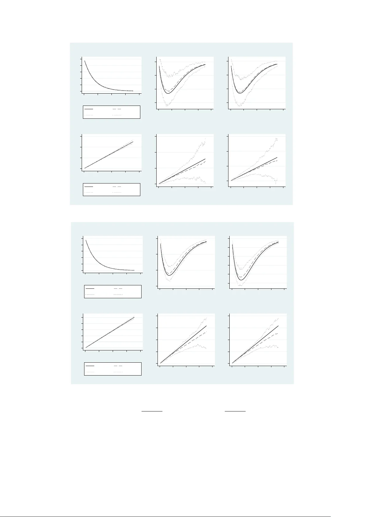
Nonparametric regression with dep enden t censoring or comp eting risks Jia-Han Shih ∗ Simon M.S. Lo † Ralf A. Wilk e ‡ Marc h 25, 2026 Abstract Single-index mo dels or time-to-ev en t mo dels are frequen tly applied in empirical researc h. These mo dels are non-identifiable in presence of unkno wn (dep enden t) cen- soring or competing risks and do not giv e informativ e results in empirical analysis un- less rather strong, non-testable restrictions hold. Little is kno wn, whether the known robustness prop erties of the single-index mo del carry o v er to mo dels with dep enden t censoring or comp eting risks. This pap er shows that the ratio of partial co v ariate ef- fects on the margins is iden tifiable in nonparametric mo dels with unkno wn dependent censoring or nonparametric comp eting risks mo dels with nonparametric dep endence structure, provided an exclusion restriction holds. Commonly used (semi)parametric ∗ National Sun Y at-sen Universit y , Departmen t of Applied Mathematics, 80424, Kaohsiung, T aiw an, E–mail: jhshih@math.nsysu.edu.tw † United Arab Emirates Univ ersit y , Departmen t of Economics and Finance, E–mail: losi- monms@y aho o.com.hk ‡ Cop enhagen Business School, Department of Economics, Porcelænsha ven 16A, 2000 F rederiksberg, DK, E–mail: rw.eco@cbs.dk mo dels for the margin and indep endent censoring, suc h as Cox prop ortional hazards, accelerated failure time or prop ortional odds mo dels, can b e used to obtain relative co v ariate effects despite their missp ecified censoring mec hanism. Several nonparamet- ric estimators for the general mo del are introduced and their numerical prop erties are studied. Keyw ords: dep endent comp eting risks, copula, identifiabilit y 1 In tro duction The non-identifiabilit y of the dependent comp eting risks mo del as shown b y Co x (1962), Tsiatis (1975) and W ang (2014) is a crux in tw o respects. First, in the absence of iden tifying restrictions, b ounds on margins and co v ariate effects are wide and uninformative (P eterson, 1976). Second, any kind of iden tifying restriction which leads to more informativ e results is non-testable. V arious approac hes to identifiabilit y ha v e b een considered in the literature. They require restrictions on either the margins, the copula or b oth. This pap er contributes to this literature b y sho wing that the ratio of tw o partial cov ariate effects on the margins are identifiable, provided an exclusion restriction holds. This is a very general result as it do es not require restrictions on the copula and the margins of the t w o risks. Man y p opular single and indep endent comp eting risks mo dels are sp ecial cases of the mo del, including the accelerated failure time, prop ortional o dds and Cox prop ortional hazards mo dels. While Li and Duan (1989) show the robustness of the single-index mo del with resp ect to a missp ecified link function, this pap er sho ws its robustness with resp ect to the unkno wn dep endent censoring distribution. An y iden tifiabilit y result hinges on a set of restrictions. F or example, the copula graphic estimator (Zheng and Klein, 1995, Carri` ere, 1995) requires a fully assumed copula but do es not restrict the margins. Hiabu et al. (2025) do not imp ose restrictions on the margins either. Under v alid exclusion restrictions, they sho w iden tifiability of the parameter of 2 an Archimedean copula. Lo and Wilke (2024) consider a semiparametric mo del for a risk of interest, while the other risk or the distribution of dep endent censoring is unspecified. They sho w that the parameter of an Archimedean copula and subsequently the margins are identifiable and estimable. Lo and Wilke (2017) do not imp ose parametric restrictions on the margins. Under the assumption that the copula do es not dep end on the cov ariates, they sho w that the sign of a cov ariate effect on the margins is often identifiable. Willems et al. (2025) consider a mo del with a semiparametric mo del for the risk of interest, unkno wn distribution of dep endent censoring and unknown censoring. Their approac h giv es b ounds for the parameters whic h often rev eal their sign. In this pap er, we in tro duce an approach that is applicable when the risk of in terest, the distribution of dep endent censoring, and the copula are completely unsp ecified. In presence of an exclusion restriction, it is shown that the ratio of tw o partial cov ariate effects on the margin of the risk of in terest is identifiable. With this result, it is p ossible to infer the relative size of the effect of a cov ariate and whether the tw o partial effects ha v e the same or opp osite sign. Our iden tifiabilit y result connects to contributions in the econometric literature which ha ve found that some patterns of single risk mo dels can b e robustly estimated when frailt y is missp ecified or omitted in the empirical sp ecification (Lancaster, 1985, Ridder, 1987). Nicoletti and Rondinelli (2010) find this for the ratio of tw o regression parameters. Mo d- elling the join t frailty distribution corresp onds to shaping the copula. Our result connects to these findings as their (semi-)parametric single risk mo dels with indep enden t censoring are sp ecial cases of our dep endent comp eting risks mo del. Our approach is more general, though, as the ratio of partial co v ariate effects can b e iden tified for an y nonparametric mo del pro vided the exclusion restriction holds. W e v erify that the identifiable ratio of partial cov ariate effects corresp onds to the ratio of regression parameters in p opular sur- viv al mo dels such as the Cox prop ortional hazards mo del, the prop ortional o dds mo del or the piecewise-constan t exp onential mo del. By comparing the ratio of partial cov ariate 3 effects from our nonparametric approach to the ratio of estimated parameters obtained b y commonly used semi- or parametric mo dels, it is p ossible to obtain evidence on whether the latter are correctly sp ecified single-index mo dels in the sense that the true mo del is a single-index mo del or that the single-index is correctly sp ecified. This can b e tested with- out kno wledge of the link function and the censoring mec hanism and without the mo del b eing identifiable. The pap er is organised as follo ws. Section 2 presen ts the mo del and the main identifia- bilit y results. Section 3 illustrates the results with sev eral examples. Section 4 introduces sev eral estimators for the ratio of partial cov ariate effects. Section 5 presen ts numerical results of monte carlo studies which demonstrate the finite-sample b eha viour and conv er- gence of the suggested approac hes. Section 6 provides empirical analysis with real data to demonstrate the applicability . 2 The mo del Let T 1 and T 2 b e the marginal contin uous surviv al times of risks 1 and 2, resp ectiv ely . W e assume a so-called exclusion restriction such that the contin uous cov ariates X and Y are included in the risk 1 margin only . Both margins ma y dep end on additional co v ariates Z , but we omit them in the mo del presentation to simplify the notation. Giv en the co v ariates X = x and Y = y , b y Sklar’s Theorem, there alw ays exists a unique copula C : [0 , 1] 2 → [0 , 1] suc h that Pr( T 1 > t 1 , T 2 > t 2 | X = x, Y = y ) = C ( S 1 ( t 1 | x, y ) , S 2 ( t 2 )) , (1) where S 1 ( t 1 | x, y ) = Pr( T 1 > t 1 | X = x, Y = y ) , S 2 ( t 2 ) = Pr( T 2 > t 2 ) . All S 1 ( t 1 | x, y ), S 2 ( t 2 ), and C ( u, v ) are nonparametric. Note that the cov ariates X and Y ha ve no impact on either the dep endence structure ( C ) or the risk 2 margin ( S 2 ). Exclusion 4 restrictions ha ve already been used in the literature to sho w identifiabilit y of the comp eting risks mo del. The mo del of Hiabu et al. (2025) also allows for nonparametric S 1 and S 2 , but requires that S 1 do es not dep end on X and S 2 do es not dep end on Y , and that C is a known Arc himedean copula with unkno wn dep endence parameter θ . They show iden tifiability of θ or the degree of dep endence b etw een risks under these restrictions. The mo del defined in (1) has suc h mild restrictions that it is not identifiable. It is w ell known that the identifiabilit y of mo dels with nonparametric margins for the t wo risks requires a kno wn copula including its parameters (Zheng and Klein, 1995, Carri` ere, 1995). The goal of the pap er can therefore not b e to show iden tifiability of S 1 , S 2 , or C . Instead, it fo cuses on other functions in relation to partial effects which can b e of high in terest in applications as w ell. F or this purp ose, we first introduce the notion of relativ e cov ariate effects, whic h remains meaningful irresp ective of any mo del assumptions (Subsections 2.1 and 2.2). Then, w e show that the relative co v ariate effects ha ve a broader in terpretation under the mo del (1), i.e., the exclusion restriction (Subsection 2.3). 2.1 Iden tifiabilit y of relativ e co v ariate effects Let T = min( T 1 , T 2 ) b e the ov erall surviv al time and its surviv al function is defined by π ( t | x, y ) = Pr( T > t | X = x, Y = y ) . (2) Differen tiating (2) with resp ect to x giv es the cov ariate effect of x on π π ′ x ( t | x , y ) = ∂ ∂ x π ( t | x, y ) , where ∂ 1 C ( u, v ) = ∂ C ( u, v ) /∂ u is the first-order partial deriv ative of the copula C with resp ect to the first argument. The first-order partial deriv ativ e of any copula exists almost ev erywhere and no condition in relation to this is added. Similarly , differentiating (2) with resp ect to y , w e obtain π ′ y ( t | x , y ) = ∂ ∂ y π ( t | x, y ) . 5 Note that the partial deriv atives π ′ x ( t | x, y ) and π ′ y ( t | x, y ) reflect how the cov ariate X and Y affect the o v erall surviv al T , as they represent the rates of c hange of π ( t | x, y ) with resp ect to X and Y , resp ectiv ely . W e define a relative co v ariate effect on π ( t | x, y ) as follo ws. Definition 1. The relative cov ariate effect based on the partial deriv ativ es of π ( t | x, y ) is defined by η π ( t, x, y ) = π ′ x ( t | x, y ) π ′ y ( t | x , y ) . (3) Prop osition 1. The r elative c ovariate effe cts η π ( t, x, y ) in (3) is identifiable. It is clear that Prop osition 1 holds since the o verall surviv al π is identifiable, and so are its partial deriv ativ es and the relativ e cov ariate effects η π ( t, x, y ). Let Λ( t | x, y ) = − log π ( t | x, y ) b e the cum ulative hazard function of the o verall surviv al. It is straigh tforward to v erify that (3) is equiv alent to η π ( t, x, y ) = Λ ′ x ( t | x , y ) Λ ′ y ( t | x, y ) , where Λ ′ x ( t | x, y ) = ∂ ∂ x Λ( t | x, y ) , Λ ′ y ( t | x, y ) = ∂ ∂ y Λ( t | x, y ) are the partial deriv ativ es of Λ. It is therefore p ossible to identify η ( t, x, y ) on the grounds of the partial deriv ativ es of π or the partial deriv ativ es of Λ. 2.2 Using the conditional exp ectation of the o v erall surviv al In surviv al or comp eting risks analysis it is common to work with surviv al or cumulativ e hazard functions and the relev an t statistical metho ds are w ell established. It turns out that the identifiabilit y result, similar to Prop osition 1, can b e written in terms of a conditional mean function as well. W riting the problem in terms of mean functions can hav e practical 6 adv an tages as it facilitates the use of a veraging approac hes to improv e the stabilit y of solutions. W e define the conditional mean of T by m ( x, y ) = E( T | X = x, Y = y ) . (4) Assume that the partial deriv atives of m ( x, y ) exist, and denote them b y m ′ x ( x, y ) = ∂ ∂ x E( T | X = x, Y = y ) , m ′ y ( x, y ) = ∂ ∂ y E( T | X = x, Y = y ) . The partial deriv ativ es m ′ x ( x, y ) and m ′ y ( x, y ) reflect ho w the co v ariate X and Y affect the conditional mean of T , as they represen t the rates of change of m ( x, y ) with resp ect to x and y , resp ectively . It is readily seen that the conditional mean m ( x, y ) is identifiable, and so are its deriv atives. In the follo wing, w e show that η π ( t, x, y ) can also be identified on the grounds of m ′ x ( x, y ) and m ′ y ( x, y ) provided it satisfies inv ariance restrictions. Let η m ( x, y ) = m ′ x ( x, y ) m ′ y ( x, y ) , (5) η = E( m ′ x ( X , Y )) E( m ′ y ( X , Y )) , (6) b e the relative co v ariate effects based on m ′ x ( x, y ) and m ′ y ( x, y ). Prop osition 2. The r elative c ovariate effe cts η m ( x, y ) in (5) and η in (6) ar e identifiable. The following theorem studies the relationships b et w een η π ( t, x, y ), η m ( x, y ), and η . Theorem 1. If η π ( t, x, y ) in (3) do es not dep end on t , then η π ( t, x, y ) = η m ( x, y ) for al l t . F urthermor e, if η m ( x, y ) in (5) do es not dep end on x and y , then η m ( x, y ) = η for al l x, y . Pr o of. If η π ( t, x, y ) do es not dep end on t , i.e., there exists a function h : R 2 → R such that η π ( t, x, y ) = h ( x, y ) for all t , and using (3), we ha v e π ′ x ( t | x, y ) = h ( x, y ) π ′ y ( t | x, y ) (7) 7 for all t . Recall that since T is a nonnegativ e random v ariable, the conditional exp ectation of T giv en X = x and Y = y can b e expressed as m ( x, y ) = Z ∞ 0 π ( t | x, y ) dt, where f T ( t | x, y ) is the conditional density of T . T ake partial deriv ativ es on b oth sides of the last equation, w e obtain m ′ x ( x, y ) = Z ∞ 0 π ′ x ( t | x, y ) dt, m ′ y ( x, y ) = Z ∞ 0 π ′ y ( t | x, y ) dt. Therefore, integrating t on b oth sides of (7) leads to m ′ x ( x, y ) = h ( x, y ) m ′ y ( x, y ) , (8) whic h implies η π ( t, x, y ) = h ( x, y ) = m ′ x ( x, y ) m ′ y ( x, y ) = η m ( x, y ) . Similarly , if η m ( x, y ) do es not dep end on x and y , i.e., there exists a constant c such that η m ( x, y ) = c for all x, y . T aking exp ectation of ( X , Y ) on b oth sides of (8) leads to E( m ′ x ( X , Y )) = c E( m ′ y ( X , Y )) , whic h implies η m ( x, y ) = c = E( m ′ x ( X , Y )) E( m ′ y ( X , Y )) = η . W e emphasise that although η π ( t, x, y ), η m ( x, y ), and η are closely related, they are iden tifiable through different routes and are each meaningful on their o wn, which ma y lead to different empirical p erformance in practice. F or instance, even if η m ( x, y ) v aries with x and y , i.e., η m ( x, y )  = η in general, estimating η remains meaningful and can still b e in terpreted. 8 2.3 The exclusion restriction W e show that η π , η m , and η in (3), (5), and (6), resp ectively , hav e a broader in terpretation under the exclusion restriction in (1), i.e., the con tinuous cov ariates X and Y are included in the risk 1 margin ( T 1 ) only . W e sho w that they are not only informative ab out the ratio of partial effects on the ov erall surviv al, but ab out the ratio of partial effects on the margin of risk 1 as well. Under the mo del (1), the ov erall surviv al function in (2) b ecomes π ( t | x, y ) = C ( S 1 ( t | x, y ) , S 2 ( t )). Then, the partial deriv ativ es of π are π ′ x ( t | x, y ) = ∂ 1 C ( S 1 ( t | x, y ) , S 2 ( t )) S ′ 1 ,x ( t | x, y ) , π ′ y ( t | x, y ) = ∂ 1 C ( S 1 ( t | x, y ) , S 2 ( t )) S ′ 1 ,y ( t | x, y ) , where ∂ 1 C ( u, v ) = ∂ C ( u, v ) /∂ u is the first-order partial deriv ative of the copula C with resp ect to the first argumen t and S ′ 1 ,x ( t | x, y ) = ∂ ∂ x S 1 ( t | x, y ) , S ′ 1 ,y ( t | x, y ) = ∂ ∂ y S 1 ( t | x, y ) are the partial deriv ativ es of S 1 . Com bining the ab o v e results, we arriv e at the conclusion that the relativ e cov ariate effect on the ov erall surviv al as defined in (3) is the same as the relativ e cov ariate effect on the margin of risk 1. In addition, we can also establish results for the risk 1 margin that are related to those in Theorem 1. Let m 1 ( x, y ) = E( T 1 | X = x, Y = y ) b e the conditional mean of T 1 . Assume that the partial deriv atives of m 1 ( x, y ) exist, and denote them by m ′ 1 ,x ( x, y ) = ∂ ∂ x E( T 1 | X = x, Y = y ) , m ′ 1 ,y ( x, y ) = ∂ ∂ y E( T 1 | X = x, Y = y ) . W e summarise the results in the follo wing theorem. 9 Theorem 2. Under the exclusion r estriction on S 2 in (1), we have η π ( t, x, y ) = S ′ 1 ,x ( t | x, y ) S ′ 1 ,y ( t | x, y ) . (9) If η π ( t, x, y ) in (3) do es not dep end on t , then η π ( t, x, y ) = η m ( x, y ) = m ′ 1 ,x ( x, y ) m ′ 1 ,y ( x, y ) holds for al l t . In addition, if η π ( t, x, y ) in (3) do es not dep end on t , x , and y , then η π ( t, x, y ) = η m ( x, y ) = η = E( m ′ 1 ,x ( X , Y )) E( m ′ 1 ,y ( X , Y )) holds for al l t, x, y . Since η π ( t, x, y ), η m ( x, y ), and η are identifiable b y Prop osition 1 and Prop osition 2, Theorem 2 implies that it is p ossible to iden tify the relative imp ortance of the co v ariates on marginal surviv al times of the risk that dep ends on them. Notably , even under the exclusion restriction, one has η m ( x, y )  = m ′ 1 ,x ( x, y ) m ′ 1 ,y ( x, y ) , η  = E( m ′ 1 ,x ( X , Y )) E( m ′ 1 ,y ( X , Y )) in general. The iden tities hold when η π ( t, x, y ) = η m ( x, y ) for all t and η π ( t, x, y ) = η for all t, x, y as stated in Theorem 2. The mo del is v ery general and nests many well-kno wn mo dels as sp ecial cases. These include single risk mo del with indep endent censoring. Let risk 2 b e the censoring time. Whenev er the censoring distribution is co v ariate inv ariant, it satisfies the exclusion restric- tion. Man y standard surviv al mo dels require a cov ariate in v arian t indep endent censoring distribution. It is obvious that these models are nested in the mo del of this pap er. The dep endence structure in a comp eting risks mo del is an alternative w ay to write a mo del with dep enden t risk sp ecific frailties (Lo et al., 2017; Lo et al., 2025). A copula mo del is therefore an alternative presentation of a dep endent frailty mo del. F railty terms b ecome in- dep enden t when there is no risk dep endence. Our iden tifiability result therefore establishes 10 the theoretical basis that certain relative patterns are iden tifiable without prior kno wledge of frailty structures or the copula in our mo del. Our findings can b e connected to previous related observ ations in the econometrics lit- erature b y Nicoletti and Rondinelli (2010), Ridder (1987) and Lancaster (1985). The latter t wo study con tin uous time single risk mo dels and sho w that the omission of frailty in their mo dels leads to a scaling bias of all co efficien ts or just the in tercept, resp ectiv ely . Nicoletti and Rondinelli (2010) consider a discrete time single risk duration mo del with frailty and indep enden t censoring. They provide numerical evidence with the help of sim ulations that the ratio of regression parameters β x and β y can b e well estimated despite missp ecification of the frailty distribution or omission of the frailty term, and despite that b oth estimated co efficien ts suffer from sizable estimation bias. It turns out that the ratio of the regres- sion parameters β x and β y corresp onds to the ratio of S ′ 1 ,x ( t | x, y ) and S ′ 1 ,y ( t | x, y ) (or m ′ 1 ,x ( x, y ) and m ′ 1 ,y ( x, y )) in these mo dels. T o establish such connection, w e employ the so-called single-index mo del for the risk 1 margin S 1 , which assumes that S 1 ( t | x , y ) dep ends solely on a linear com bination of x and y , namely the single-index xβ x + y β y . The following theorem gives an equiv alen t statement of the single-index assumption. Theorem 3. L et T 1 b e a c ontinuous r andom variable and ( β x , β y )  = (0 , 0) b e the r e gr ession p ar ameters on the c ontinuous c ovariates X and Y , r esp e ctively. Then, S ′ 1 ,x ( t | x, y ) = β x β y S ′ 1 ,y ( t | x, y ) (10) for al l t, x, y if and only if ther e exists a function G ( t, a ) such that: (i) for e ach a , t 7→ G ( t, a ) is a c ontinuous survival function; (ii) for e ach t , a 7→ G ( t, a ) is differ entiable; and S 1 ( t | x, y ) = G ( t, xβ x + y β y ) (11) for al l t, x, y . 11 Pr o of. Define tw o new v ariables: a = xβ x + y β y , b = xβ y − y β x . The ab ov e c hange of v ariables is inv ertible and we can express ( x, y ) in terms of ( s, t ) by x = x ( a, b ) = aβ x + bβ y β 2 x + β 2 y , y = y ( a, b ) = aβ y − bβ x β 2 x + β 2 y . This means that ev ery ( a, b ) corresp onds to exactly one ( x, y ), and vice versa. F or a fixed t , define M ( t, a, b ) = S 1 ( t | x ( a, b ) , y ( a, b )) . Since S 1 ( t | x, y ) is differen tiable with resp ect to x and y , and the maps b 7→ x ( a, b ) and b 7→ y ( a, b ) are smo oth for each fixed a , by the chain rule, ∂ ∂ b M ( t, a, b ) = S ′ 1 ,x ( t | x, y ) ∂ ∂ b x ( a, b ) + S ′ 1 ,y ( t | x, y ) ∂ ∂ b y ( a, b ) = 1 β 2 x + β 2 y ( S ′ 1 ,x ( t | x, y ) β y − S ′ 1 ,y ( t | x, y ) β x ) . If (10) holds, we arriv e that ∂ M ( t, a, b ) /∂ b = 0 for all a, b , that is, the function M ( t, a, b ) do es not dep end on b . Consequen tly , there exists a function G ( t, a ) such that a 7→ G ( t, a ) is differentiable and M ( t, a, b ) = G ( t, a ) for all a, b . W e obtain S 1 ( t | x, y ) = G ( t, a ) = G ( t, xβ x + y β y ) , hence t 7→ G ( t, a ) is a contin uous surviv al function. The other direction is obvious. Theorem 3 rev eals that the relationship (10) is inheren t in the single-index model. T ogether with Prop osition 1 and Theorem 2, w e obtain the follo wing p o werful result, whic h co vers a wide range of mo dels in the literature. Corollary 1. Under the exclusion r estriction, if the risk 1 mar gin S 1 fol lows the single- index mo del in (11), the r atio of r e gr ession p ar ameters β x and β y is identifiable, pr ovide d 12 that ( β x , β y )  = (0 , 0) . In addition, β x β y = η π ( t, x, y ) = η m ( x, y ) = η for al l t, x, y , wher e η π ( t, x, y ) , η m ( x, y ) , and η ar e define d in (3)–(6), r esp e ctively. Corollary 1 sho ws that the identit y β x /β y = η π ( t, x, y ) = η m ( x, y ) = η holds under t w o conditions: (i) the risk 1 margin S 1 follo ws a single-index mo del with contin uous cov ariates X and Y and a prop er link function G ; and (ii) the risk 2 margin S 2 is cov ariate-inv ariant. Imp ortan tly , this result holds regardless of other conditions, such as the sp ecific form of G or the dependence structure betw een the tw o risks. The conditions (i) and (ii) are rather mild and are satisfied by man y well-kno wn statistical regression mo dels. Corollary 1 therefore implies that η is inv ariant in these mo dels and can b e easily obtained by dividing the parameters on the cov ariates without kno wing the link function and the copula. It is already kno wn that the parameters of single-index mo dels with unkno wn link function are iden tifiable up to a multiplicativ e scalar (Li and Duan, 1989). Our result generalises this to situations with dep endent censoring or dep endent comp eting risks. 3 Examples W e illustrate Corollary 1 using prominen t examples satisfying β x /β y = η , where S 1 follo ws p opular and w ell-known regression mo dels, S 2 is an unknown but cov ariate-inv ariant cen- soring distribution, and C is unkno wn as well. An example of β x /β y  = η is also provided. 3.1 Single-index mo dels Example 1 (Co x PH) . The Cox prop ortional hazards (PH) mo del is given b y S 1 ( t | x , y ) = S 10 ( t ) exp( xβ x + y β y ) , where S 10 ( t ) = S 1 ( t | 0 , 0) is the baseline surviv al function of the risk 1 margin. 13 Example 2 (PO) . The prop ortional o dds (PO) mo del is given by S 1 ( t 1 | x, y ) = S 10 ( t ) S 10 ( t ) + (1 − S 10 ( t )) exp( xβ x + y β y ) . Example 3 (AFT) . The accelerated failure time (AFT) mo del is giv en by S 1 ( t | x, y ) = S 10 ( t exp( xβ x + y β y )) . Example 4 (Piecewise exp onen tial) . Consider a piecewise exp onential (constant hazard) mo del on each unit interv al with its hazard function giv en by λ 1 ( s | x, y , ϵ ) = log (1 + e − xβ x − y β y + f ( t ) − ϵ ) , s ∈ [ t − 1 , t ) , t = 1 , 2 , . . . , where f ( t ) is a deterministic function of elapsed duration and ϵ is an individual random effect. F or clarity , w e denote z t = xβ x + y β y − f ( t ) + ϵ, p t = 1 1 + e z t . Then the cumulativ e hazard is expressed as Λ 1 ( t | x, y , ϵ ) = ( t − ⌊ t ⌋ ) λ 1 ( t | x, y , ϵ ) + ⌊ t ⌋ X k =1 λ 1 ( k | x, y , ϵ ) = ( t − ⌊ t ⌋ ) log(1 + e − z t ) + ⌊ t ⌋ X k =1 log(1 + e − z k ) = − ( t − ⌊ t ⌋ ) log(1 − p t ) − ⌊ t ⌋ X k =1 log(1 − p k ) , where ⌊ x ⌋ denotes the largest integer that is less or equal to x . Thus, the surviv al function is S 1 ( t | x, y , ϵ ) = exp   ( t − ⌊ t ⌋ ) log(1 − p t ) + ⌊ t ⌋ X k =1 log(1 − p k )   = (1 − p t ) t −⌊ t ⌋ ⌊ t ⌋ Y k =1 (1 − p k ) . Note that p t is a function of xβ x + y β y and so is S 1 ( t | x, y , ϵ ). 14 In fact, the piecewise exp onential mo del corresp onds to the discrete duration mo del in Nicoletti and Rondinelli (2010). T o see this, note that for any in teger t , we ha ve Pr( T 1 ≥ t | T 1 ≥ t − 1 , X = x, Y = y , E = ϵ ) = Pr( T 1 ≥ t | X = x, Y = y , E = ϵ ) Pr( T 1 ≥ t − 1 | X = x, Y = y , E = ϵ ) = S 1 ( t | x, y , ϵ ) S 1 ( t − 1 | x, y , ϵ ) = 1 − p t . Therefore, the discrete hazard in the in terv al [ t − 1 , t ) is Pr( T 1 ∈ [ t − 1 , t ) | T 1 ≥ t − 1 , X = x, Y = y , E = ϵ ) = Pr( T 1 < t | T 1 ≥ t − 1 , X = x, Y = y , E = ϵ ) = 1 − Pr( T 1 ≥ t | T 1 ≥ t − 1 , X = x, Y = y , E = ϵ ) = p t = 1 1 + e z t , whic h is the same as Equations (3)–(4) in Nicoletti and Rondinelli (2010). Note that the random effect E do es not affect the result as long as ∂ ∂ x E E { S 1 ( t | x, y , E ) } = E E  ∂ ∂ x S 1 ( t | x, y , E )  . It is ob vious that the models in Examples 1–4 are included in the single-index mo del (11), hence the ratio β x /β y is iden tifiable and equal to relativ e co v ariates effects under the exclusion restriction by Corollary 1. 3.2 Non-single-index mo del Example 5 (Two-Hazards) . W e consider a t wo-hazards additive mo del in which the marginal hazard for risk 1 is the sum of a time-linear PH term driven by X and a time- constan t PH term driv en by Y : λ 1 ( t | x, y ) = a 1 e xβ x t + b 1 e y β y , where a 1 , b 1 > 0 are parameters. The corresp onding margin S 1 is S 1 ( t | x, y ) = exp  −  1 2 a 1 e xβ x t 2 + b 1 e y β y t  . (12) 15 Ob viously , the mo del (12) does not b elong to the single-index mo del in (11). By Theorem 1, w e differentiate (12) with resp ect to b oth x and y and tak e their ratio to obtain η π ( t, x, y ) = S ′ 1 ,x ( t | x, y ) S ′ 1 ,y ( t | x, y ) = β x β y a 1 e xβ x 2 b 1 e y β y t  = β x β y , whic h demonstrates that (10) do es not hold without those conditions in Theorem 3. In this case, the meaning of the ratio β x /β y is unclear, ho w ever, the relativ e cov ariate effect η π ( t, x, y ) can alwa ys b e in terpreted through the o verall surviv al π based on its own defi- nition in (3), and through the risk 1 margin S 1 based on the relationship in (9) under the exclusion restriction. Since η π ( t, x, y ) dep ends on t in this mo del, η π ( t, x, y )  = η m ( x, y )  = m ′ 1 ,x ( x, y ) m ′ 1 ,y ( x, y ) and η m ( x, y ) can only be in terpreted in terms of the o v erall surviv al π (compare (5)). T o see that η m ( x, y ) is a complicated function of S 2 and C in this mo del, w e pro vide an example. Let S 2 ( t ) = exp  −  1 2 a 2 t 2 + b 2 t  , where a 2 , b 2 > 0 are parameters. Also, let C b e the Clayton copula C θ ( s 1 , s 2 ) = ( s − θ 1 + s − θ 2 − 1) − 1 /θ with dep endence parameter θ > 0. Then, one can ev aluate η m ( x, y ) = m ′ x ( x, y ) m ′ y ( x, y ) = Z ∞ 0 ∂ 1 C θ ( S 1 ( t | x , y ) , S 2 ( t )) S ′ 1 ,x ( t | x, y ) dt Z ∞ 0 ∂ 1 C θ ( S 1 ( t | x, y ) , S 2 ( t )) S ′ 1 ,y ( t | x, y ) dt (13) n umerically and it dep ends on a 2 , b 2 , and θ , i.e., the parameters of S 2 and C θ . T o verify this analytically , we derive η m ( x, y ) in the limit as θ → 0, where C θ reduces to the indep endence copula. In this case, we hav e π ( t | x, y ) = exp  −  A ( x ) t 2 + B ( y ) t  , where A ( x ) =  a 1 e xβ x + a 2  / 2 and B ( y ) = b 1 e y β y + b 2 . After a lengthy calculation, we get m ( x, y ) = Z ∞ 0 π ( t | x, y ) dt = r π 2 A ( x ) exp  B ( y ) 4 A ( x )  erfc B ( y ) 2 p A ( x ) ! , 16 where erfc( z ) = 2 √ π Z ∞ z e − u 2 du. Differen tiate m ( x, y ) with resp ect to x and y and take their ratio, we ha v e η m ( x, y ) = m ′ x ( x, y ) m ′ y ( x, y ) = β x β y a 1 e xβ x 2 b 1 e y β y (2 A ( x ) + B ( y )) 2 m ( x, y ) − B ( y ) 2 A ( x )(1 − B ( y ) m ( x, y )) , whic h clearly dep ends on a 2 and b 2 , i.e., the parameters of S 2 . 4 Estimation The ratio η π ( t, x, y ) is iden tifiable from π ( t | x, y ) and its deriv ativ es, or Λ( t | x, y ) and its deriv ativ es. The ratio η m ( x, y ) is identifiable from the conditional mean function m ( x, y ) and its deriv ativ es. The ratio η is iden tifiable from the deriv atives of m ( x, y ) after applying an av eraging step o v er the joint distribution of ( X , Y ). In this section, w e consider ap- propriate nonparametric estimation approaches for the unkno wn functionals. Estimation of π ( t | x, y ) and its deriv ativ es has already b een considered in Hiabu et al. (2025). The estimators for Λ( t | x, y ) and m ( x, y ) and their deriv ativ es are stated b elo w. The data consist of a random sample ( t i , x i , y i ) for i = 1 , . . . , N . The cum ulative o v erall hazard function is nonparametric and can b e recov ered from the o verall hazard function in the usual wa y . W e therefore first define the nonparametric estimator for λ ( t | x, y ) = f ( t | x, y ) /π ( t | x, y ), where f is the densit y of T . A nonparametric estimator is ˆ λ ( t | x, y ) = P N i =1 1 I( t i = t ) K h x ( x − x i ) K h y ( y − y i ) P N i =1 1 I( t i > t ) K h x ( x − x i ) K h y ( y − y i ) , where 1 I( · ) is the indicator function, K h x ( x ) = K ( x/h x ) /h x is a Kernel function and h x is the bandwidth. K h y ( y ) is analogously defined. The estimator utilises a pro duct Kernel for the tw o-dimensional smo othing problem. The estimator for Λ( t | x, y ) is the Nelson-Aalen t yp e estimator ˆ Λ( t | x, y ) = X j | t j ≤ t ˆ λ ( t j | x, y ) , 17 where the t j s are the distinct realisations of T . The estimator for Λ ′ x ( t | x, y ) is ˆ Λ ′ x ( t | x , y ) = n P N i =1 1 I { t i > t } K ′ h x ( x − x i ) K h y ( y − y i ) o n P N i =1 K h x ( x − x i ) K h y ( y − y i ) o n P N i =1 K h x ( x − x i ) K h y ( y − y i ) o 2 − n P N i =1 K ′ h x ( x − x i ) K h y ( y − y i ) o n P N i =1 1 I { t i > t } K h x ( x − x i ) K h y ( y − y i ) o n P N i =1 K h x ( x − x i ) K h y ( y − y i ) o 2 , where K ′ h ( x ) denotes the partial deriv ative of K h ( x ) with resp ect to x . ˆ Λ ′ y ( t | x, y ) is the estimator for Λ ′ y ( t | x, y ) and is defined analogously . Once these estimates are av ailable, the ratio η π ( t, x, y ) in (3) can b e estimated by ˆ η π ( t, x, y ) = ˆ π ′ x ( t | x, y ) ˆ π ′ y ( t | x , y ) (14) or ˆ η Λ ( t, x, y ) = ˆ Λ ′ x ( t | x, y ) ˆ Λ ′ y ( t | x, y ) . (15) Hiabu et al. (2025) state the Kernel estimator for ˆ π ′ x and ˆ π ′ y and establish w eak consistency under appropriate bandwidth and Kernel c hoice (Hiabu et al., 2025, Corollary 1). The w eak consistency of ˆ Λ ′ x and ˆ Λ ′ y can b e established in an analogous w ay . The estimators ˆ η π and ˆ η Λ are the av erages of the ratio of t wo weakly consisten t nonparametric estimates and therefore inherit this prop ert y . These ratios can resp ond very strongly to finite-sample biases, though. Hiabu et al. (2025) study similar ratios of estimators and observ e p o or finite- sample prop erties. They in tro duce trimming rules to impro ve finite sample b eha viour. In our implemen tation, w e also w ork with trimming rules that restrict the range of t and exclude ev aluations of the ratio when the denominator is small. Subsection 2.2 defines the ratio η m ( x, y ) on the basis of the deriv atives of conditional mean. Recall that the conditional exp ectation m ( x, y ) in (4) can b e directly estimated b y the Nadaray a–W atson estimator which is defined as ˆ m ( x, y ) = P N i =1 t i K h x ( x − x i ) K h y ( y − y i ) P N i =1 K h x ( x − x i ) K h y ( y − y i ) . (16) 18 The Nadaray a-W atson estimator is kno wn to b e consistent under appropriate bandwidth and Kernel function choice. A natural estimator for m ′ x ( x, y ) can be obtained by taking partial deriv ative of ˆ m x ( x, y ) in (16) with resp ect to x , namely , ˆ m ′ x ( x, y ) = n P N i =1 t i K ′ h x ( x − x i ) K h y ( y − y i ) o n P N i =1 K h x ( x − x i ) K h y ( y − y i ) o n P N i =1 K h x ( x − x i ) K h y ( y − y i ) o 2 − n P N i =1 t i K h x ( x − x i ) K h y ( y − y i ) o n P N i =1 K ′ h x ( x − x i ) K h y ( y − y i ) o n P N i =1 K h x ( x − x i ) K h y ( y − y i ) o 2 . (17) Similarly , a nonparametric estimator for m ′ y ( x, y ) is ˆ m ′ y ( x, y ) = n P N i =1 t i K h x ( x − x i ) K ′ h y ( y − y i ) o n P N i =1 K h x ( x − x i ) K h y ( y − y i ) o n P N i =1 K h x ( x − x i ) K h y ( y − y i ) o 2 − n P N i =1 t i K h x ( x − x i ) K h y ( y − y i ) o n P N i =1 K h x ( x − x i ) K ′ h y ( y − y i ) o n P N i =1 K h x ( x − x i ) K h y ( y − y i ) o 2 . (18) By taking the ratio of (17) and (18), one can estimate η m ( x, y ) in (5) b y ˆ η m ( x, y ) = ˆ m ′ x ( x, y ) ˆ m ′ y ( x, y ) = S t,dx S ( x, y ) − S t ( x, y ) S dx ( x, y ) S t,dy ( x, y ) S ( x, y ) − S t ( x, y ) S dy ( x, y ) , where S t,dx ( x, y ) = n X i =1 t i K ′ h x ( x − x i ) K h y ( y − y i ) , S dx ( x, y ) = n X i =1 K ′ h x ( x − x i ) K h y ( y − y i ) , S t,dy ( x, y ) = n X i =1 t i K h x ( x − x i ) K ′ h y ( y − y i ) , S dy ( x, y ) = n X i =1 K h x ( x − x i ) K ′ h y ( y − y i ) , S t ( x, y ) = n X i =1 t i K h x ( x − x i ) K h y ( y − y i ) , S ( x, y ) = n X i =1 K h x ( x − x i ) K h y ( y − y i ) . Lastly , the ratio η in (6) can b e estimated by using the ratio of the empirical mean of (17) and (18). The estimator is ˆ η = P n i =1 ˆ m ′ x ( x i , y i ) P n i =1 ˆ m ′ y ( x i , y i ) . (19) When the mo del is the single-index mo del in (11), η π ( t, x, y ) = η m ( x, y ) = η for all t, x, y and it is p ossible to compare the estimates. ˆ η is exp ected to b e less sensitive to finite- sample biases than the a verages of ˆ η π ( t, x, y ) or ˆ η m ( x, y ) ov er t, x, y . This is b ecause ˆ η 19 is constructed as a ratio of a v eraged estimates in the numerator and denominator, rather than as an a v erage of the ratios. In summary , η π ( t, x, y ), η m ( x, y ) and η can b e estimated without sp ecifying the copula and without sp ecifying the mo dels for S 1 and S 2 . The only other single risk approach that do es not require a mo del for the copula has b een developed by Willems et al. (2025), but it only partially iden tifies the mo del parameters. Although all estimators for η π ( t, x, y ), η m ( x, y ) and η are consistent under an appropriate bandwidth choice, the in tro duced approaches likely differ in their finite sample prop erties, whic h are studied in the next section with the help of simulations. 5 Sim ulations This section presen ts the results of Monte Carlo sim ulations to assess the finite-sample p er- formance of the suggested approaches. The fo cus is on the estimation of β x /β y . In the first part, the differen t nonparametric estimators of Section 4 are applied to estimate the relative co v ariate effect. In the second part, the nonparametric approach is compared to commonly used (semi)parametric single-index mo dels under correct and incorrect sp ecification. Estimation of η π , η m and η . Sev eral designs for different copulas and θ s are considered. T o assess the differences in finite sample b ehaviour, estimation is done b y using the esti- mators for Λ, π and m and their resp ectiv e deriv atives. The simulation designs are similar to those in Hiabu et al. (2025) to allow for comparability . Stata 16MP is used for these sim ulations. The margins of b oth risks are W eibull models with cumulativ e baseline hazards Λ 0 j ( t ) = λ j t η j with ( λ 1 , η 1 , λ 2 , η 2 ) = (0 . 5 , 1 , 1 , 1). The cov ariate function for risk 1 is exp( xβ x + y β y ) with ( β x , β y ) = (1 , 1). Therefore S 1 ( t | x, y ) = exp {− 0 . 5 exp( x + y ) } and S 2 ( t ) = exp( − 1). The copula is either the Cla yton copula C θ ( s 1 , s 2 ) = ( s − θ 1 + s − θ 2 − 1) − 1 /θ with θ > 0 or 20 the Gum b el copula C θ ( s 1 , s 2 ) = exp[ −{ ( − log s 1 ) θ + ( − log s 2 ) θ } 1 /θ ] with θ ∈ [1 , ∞ ). The sim ulations are done for tw o different degrees of dep endence with Kendall- τ ∈ { 0 . 1 , 0 . 8 } , where one is rather w eak and one is rather strong. The data generating pro cess (DGP) requires the conditional distribution function of the second v ariable giv en the first under the sp ecified copula, namely , F ( s 2 | s 1 ) = ∂ 1 C θ ( s 1 , s 2 ), as well as its inv erse F − 1 ( v 2 | s 1 ). The pro cess of generating the data consists of 4 steps: 1. Generate tw o uniform random v ariables s 1 and v 2 on [0 , 1] with N indep enden t ran- dom draws. 2. Obtain N realisations of s 2 b y computing F − 1 ( v 2 | s 1 ): • Clayton copula: s 2 =  1 − s − θ 1 + ( v 2 s θ +1 1 ) − θ/ ( θ +1)  − 1 /θ . • Gumbel copula: s 2 is obtained numerically b y computing the ro ot of F ( s 2 | s 1 ) − v 2 = 0 . 3. Randomly generate a sample of size N of indep enden t x and y with marginal distri- bution N (0 , 1). Obtain durations t 1 and t 2 giv en x and y by in verting the marginal W eibull surviv al: t 1 = [ − log ( s 1 ) /λ η 1 1 / exp( β x x + β y y )] 1 /η 1 , t 2 = [ − log ( s 2 ) /λ η 2 2 ] 1 /η 2 . 4. Generate observ ed minimum duration and observed risk by relating t 1 and t 2 . The DGP results in b et w een 63%–79% of the t i corresp onding to realisations of T 1 , and the rest to T 2 , dep ending on the choice of C and τ . Sim ulations are conducted for different sample sizes N = 5 , 000, N = 10 , 000, and N = 25 , 000 with 100 runs. The Epanec hniko v 21 Kernel is used for the nonparametric smo othing. The sensitivity of results with resp ect to the bandwidth choice is chec k ed by setting h x = h y = h to either 0 . 2 or 0 . 3. In this mo del, η π ( t, x, y ) = η m ( x, y ) = η = β x /β y = 1 for all t , x , y . All presen ted estimation approaches of Section 4 are therefore applicable. Hiabu et al. (2025) pro vide numerical evidence of the finite-sample p erformance of a related estimator of a ratio of partial deriv ativ es of π . Their results suggest that a large dataset of sev eral 10 , 000 observ ations is required in an application. This is confirmed by our simulations for the estimation of η π . In our implemen tation, w e ev aluate ˆ η π ( t, x, y ) and ˆ η Λ ( t, x, y ) in (14) and (15), resp ectiv ely , on a equidistan t grid for t and tak e the a v erage o v er these grid p oin ts for x = ¯ x = P n i =1 x i /n and y = ¯ y = P n i =1 y i /n , namely , ˆ η π ( ¯ x, ¯ y ) = G − 1 G X g =1 ˆ η π ( t g , ¯ x, ¯ y ) = G − 1 N X g =1 ˆ π ′ x ( t g | ¯ x, ¯ y ) ˆ π ′ y ( t g | ¯ x, ¯ y ) , ˆ η Λ ( ¯ x, ¯ y ) = G − 1 G X g =1 ˆ η Λ ( t g , ¯ x, ¯ y ) = G − 1 N X g =1 ˆ Λ ′ x ( t g | ¯ x, ¯ y ) ˆ Λ ′ y ( t g | ¯ x, ¯ y ) , where g = 1 , . . . , G are the grid points on the supp ort of t with G = 500. Note that the a veraging is not done in the cov ariates to restrict the lo cal estimation to areas with the greatest marginal densities of x and y and to sp eed up estimation. As already observed by Hiabu et al. (2025), this impro ves the n umerical stabilit y of the results. In a similar fashion, w e also ev aluate ˆ η m ( x, y ) at x = ¯ x n and y = ¯ y n , namely , ˆ η m ( ¯ x, ¯ y ), which corresp ond to the cen ter of mass of the cov ariates. The sim ulation results for ˆ η are given in T able 1. The mean of the realisations of ˆ η is very close to the true v alue for all sample sizes. The p ercen tiles of the distribution of estimates get closer to the true v alues when N increases. This sho ws desirable prop erties. A t the same time, the in terv als get rather wide for N = 5 , 000 which suggests that this approach requires at least several thousand observ ations. T aking the a verage b efore division instead of a v eraging the ratios has therefore considerably impro v ed the finite-sample p erformance. There is no need to choose v alues of t , x and y for the estimation because the estimator 22 a verages ov er all observ ations. T able 1: Simulation results for ˆ η using P i ˆ m ′ x ( x i , y i ) / P i ˆ m ′ y ( x i , y i ) under the Gum b el or Cla yton copula with τ = 0 . 1 or τ = 0 . 8. T rue η = 1. Gumbel Clayton h = 0 . 2 h = 0 . 3 h = 0 . 2 h = 0 . 3 τ = 0 . 1 N = 5 , 000 mean ˆ η 0 . 9867 0 . 9918 0 . 9886 0 . 9860 5th, 95th p ercentile of ˆ η [0 . 7263 , 1 . 2303] [0.7824,1.2382] [0.7062,1.2499] [0 . 7567 , 1 . 2159] N = 10 , 000 mean ˆ η 1 . 0015 0 . 9984 0 . 9995 1 . 0056 5th, 95th p ercentile of ˆ η [0 . 8342 , 1 . 2217] [0.8483,1.2278] [0.8050,1.2290] [0 . 8344 , 1 . 2056] N = 25 , 000 mean ˆ η 1 . 0097 1 . 0110 0 . 9806 0 . 9823 5th, 95th p ercentile of ˆ η [0 . 8972 , 1 . 1267] [0.9058,1.1359] [0.8761,1.1122] [0 . 8780 , 1 . 1127] τ = 0 . 8 N = 5 , 000 mean ˆ η 0 . 9496 0 . 9676 1 . 0136 1 . 0095 5th, 95th p ercentile of ˆ η [0 . 5432 , 1 . 5528] [0.6242,1.5534] [0.5575,1.5842] [0 . 5322 , 1 . 5892] N = 10 , 000 mean ˆ η 1 . 0063 1 . 0044 0 . 9990 1 . 0103 5th, 95th p ercentile of ˆ η [0 . 7037 , 1 . 3765] [0.7074,1.4080] [0.6684,1.4482] [0 . 7028 , 1 . 4590] N = 25 , 000 mean ˆ η 1 . 0267 1 . 0332 0 . 9813 0 . 9821 5th, 95th p ercentile of ˆ η [0 . 7714 , 1 . 2865] [0.7857,1.2700] [0.7691,1.2094] [0 . 7719 , 1 . 2314] The results for the estimators ˆ η π ( ¯ x, ¯ y ), ˆ η Λ ( ¯ x, ¯ y ) and ˆ η m ( ¯ x, ¯ y ) are given in Supplemen tary Material. When the estimation uses π or Λ and their deriv ativ es, estimation is done on an equidistan t grid for t with 500 p oin ts on [0 . 04 , 3 . 55]. In these cases, appropriate trimming rules are applied to av oid instability of results when there are low observ ation num b ers 23 in some areas of the supp ort or the denominators are very small. No trimming in the t dimension is required when estimation is based on the conditional mean function. T ables S3–S6 presen t the results for different bandwidths h , τ and copulas. It is apparen t that these approac hes require several 10,000 observ ations to get some stable results and that ˆ η has the b est p erformance. A selection of estimated nonparametric ˆ π and ˆ Λ and their deriv atives are shown in Figure S1 to illustrate the role of the bandwidth choice. F or h = 0 . 2, the bias is smaller but the p ercen tiles of the distribution are wider spread, showing the greater v ariance of the estimates. Figure S2 sho ws results for the distribution of the estimated ˆ η π ( t, ¯ x, ¯ y ) as a function of t . It is apparent that in some areas of the supp ort of t , the estimates are v ery noisy . A similar observ ation has already b een made in Hiabu et al. (2025). T o address this and impro ve the qualit y of the estimates, w e trim the supp ort of t to [0 . 05 , 2 . 5] in the case of the Gumbel copula and [0 . 05 , 0 . 5] in the case of Cla yton. By doing so, w e trim the righ t end of the t where estimates are found to b e more noisy mainly due to less observ ations. This is denoted as trimming I: b oundary trimming in the tables and is made visible by the dotted vertical lines in Figure S2 for the Gumbel copula. An additional trimming rule ignores grid p oints for which denominator in ˆ η π ( t, ¯ x, ¯ y ) is to o close to zero. This is when ˆ Λ y or ˆ π y are less than 0 . 1 as a small estimation bias in this estimates leads to a sizable bias of ˆ η π ( ¯ x, ¯ y ) and ˆ η Λ ( ¯ x, ¯ y ). This is denoted as trimming rule II: boundary and denominator trimming in the tables. Estimation on the grounds of the conditional mean functions do es not require this trimming. T o sum up, the sim ulation results confirm that the suggested estimators conv erge to their true v alues and their v ariances decrease as the sample size N increases. They also sho w that the purely nonparametric approac h require samples of ideally at least several thousand observ ations. The preferable approach is the estimator ˆ η in (19), whic h divides the sample av erages of nonparametric mean regression estimates. The approaches that 24 a verage the ratio of tw o nonparametric estimates hav e considerably worse prop erties and require 10,000s of observ ations. Comparison with (semi)parametric single-index mo dels. The previous results sug- gested that the nonparametric approaches lac k the precision of (semi)parametric approac hes under correct sp ecification and require larger data sets. Their adv antage is that they are consisten t for η = E[ m ′ x ( X , Y )] / E[ m ′ y ( X , Y )] in (6), but not for β x /β y under w eaker restric- tions, in particular when the mo del is not a single-index mo del or when the single-index comp onen t is missp ecified. In the following, w e compare the p erformance of the estimated η on the grounds of the nonparametric estimator in (19) and the ratio of estimated co effi- cien ts of the single-index mo dels: the semiparametric Cox PH mo del, the AFT mo del with W eibull distribution and the PO mo del (compared Section 3). When the single-index mo del is correctly sp ecified, it is more efficient and therefore preferable o ver the nonparametric ap- proac h. F or non-single-index mo dels, the (semi)parametric and the nonparametric cannot b e used to consisten tly estimate β x /β y , although the nonparametric approach still consis- ten tly estimates η . When the single-index comp onen t is missp ecified, the nonparametric approac h is consistent for m ′ x ( x, y ) /m ′ y ( x, y ) = η π ( x, y ) and η , but not for β x /β y as η π ( x, y ) dep ends on x and y . W e apply the DGP of the W eibull mo del of the previous simulations as the correctly sp ecified mo del. The DGPs that violates the single-index prop ert y is the Tw o-hazards mo del of Example 5 in Subsection 3.2 with ( a 1 , b 1 , a 2 , b 2 ) = (1 , 1 , 0 . 5 , 1) and ( β x , β y ) = (1 , 1). The mo del with missp ecified single-index is the W eibull mo del with co- v ariate function exp( β x + β y + β x 2 x 2 ) for risk 1 with ( β x , β y , β x 2 ) = (1 , 1 , 2), but the co v ariate function exp( β x + β y ) is used for the estimation of the (semi)parametric mo dels. The sim u- lations are run for N = 5 , 000 and 25 , 000 and use the Clayton copula with Kendall- τ = 0 . 8. The bandwidth is selected by 10-fold Cross-V alidation. The statistical softw are R V.4.5.2 is used for these simulations. 25 T able 2: Simulation results for ˆ η under the Clayton copula with τ = 0 . 8. W eibull AFT is a single-index mo del, while Tw o-Hazards is a non-single-index mo del and W eibull AFT x 2 is a single-index mo del with missp ecified cov ariate function. Estimator \ DGP (a) (b) (c) W ei bull AFT Two-Hazards W eibull AFT x 2 η = β x /β y = 1 η  = β x /β y = 1 η  = β x /β y = 1 N = 5 , 000 Nonparametric mean ˆ η 0 . 9971 0 . 6487 0 . 6104 5th, 95th p ercentile of ˆ η [0 . 7393 , 1 . 3452] [0 . 4507 , 0 . 8619] [0 . 4391 , 0 . 7776] Semiparametric Cox PH mean ˆ η 0 . 9952 0 . 6254 1 . 0442 5th, 95th p ercentile of ˆ η [0 . 9548 , 1 . 0397] [0 . 5587 , 0 . 6872] [0 . 8968 , 1 . 2069] Parametric W eibull AFT mean ˆ η 0 . 9952 0 . 6137 1 . 0489 5th, 95th p ercentile of ˆ η [0 . 9539 , 1 . 0429] [0 . 5494 , 0 . 6727] [0 . 9003 , 1 . 2128] Semiparametric PO mean ˆ η 0 . 9935 0 . 5693 0 . 8861 5th, 95th p ercentile of ˆ η [0 . 9454 , 1 . 0429] [0 . 5123 , 0 . 6278] [0 . 7566 , 1 . 0346] N = 25 , 000 Nonparametric mean ˆ η 1 . 0079 0 . 6713 0 . 5879 5th, 95th p ercentile of ˆ η [0 . 8982 , 1 . 1312] [0 . 5925 , 0 . 7781] [0 . 5124 , 0 . 6534] Semiparametric Cox PH mean ˆ η 1 . 0006 0 . 6330 1 . 0559 5th, 95th p ercentile of ˆ η [0 . 9803 , 1 . 0181] [0 . 6044 , 0 . 6584] [0 . 9909 , 1 . 1310] Parametric W eibull AFT mean ˆ η 1 . 0008 0 . 6204 1 . 0611 5th, 95th p ercentile of ˆ η [0 . 9797 , 1 . 0183] [0 . 5927 , 0 . 6459] [0 . 9946 , 1 . 1356] Semiparametric PO mean ˆ η 0 . 9997 0 . 5762 0 . 8972 5th, 95th p ercentile of ˆ η [0 . 9785 , 1 . 0185] [0 . 5513 , 0 . 5996] [0 . 8363 , 0 . 9629] 26 The results are shown in T able 2. Column (a) is the correctly sp ecified single-index mo del. Column (b) is the non-single-index mo del and column (c) is the mo del with the missp ecified single-index. It is apparent from (a) that all metho ds are consisten t for η and the con ven tional (semi)parametric mo dels are more efficien t when the underlying mo del is a correctly sp ecified single-index mo del. It illustrates that the robustness prop erty of the single-index mo dels (Li and Duan, 1989) may carry ov er to settings with (dep enden t) censoring or comp eting risks. The results in (b) sho w that all mo dels do not consisten tly estimate the ratio of parameters and they conv erge to differen t p oin ts except the Co x PH and the W eibull AFT mo dels whic h give v ery similar results. The nonparametric approach con verges in probabilit y to η = E[ m ′ x ( X , Y )] / E[ m ′ y ( X , Y )] = 0 . 6759 in this setup, where the true v alue is approximated n umerically using the Monte Carlo metho d to ev aluate the exp ected v alues of the numerator and denominator of (13). The previous simulations hav e already confirmed that the nonparametric estimator for η π ( x, y ) is consisten t and w e omit the reporting. The results in (c) for the misspecified cov ariate function in a single-index mo del show a similar pattern. The true v alue η = 0 . 5617 in this setup is approximated n umerically as well. The fact that the differen t estimators conv erge to differen t p oints when the mo del is not a correctly sp ecified single-index mo del, pro vides evidence against this assumption. A b o otstrap-based test can b e utilised to detect systematic differences in the ˆ η s of the different approaches. 6 Empirical applications W e present t wo applications to put our framew ork in to practice. One data set is from economics to study unemploymen t duration, the other data set is medical data. It contains patien t surviv al times in hospitals. F or both applications, w e first obtain the nonparametric 27 estimator ˆ η in (19). Then, we also compute the ratios of regression parameters ˆ η Cox = ˆ β Cox x ˆ β Cox y , ˆ η PO = ˆ β PO x ˆ β PO y , where ˆ β Cox x and ˆ β Cox y ( ˆ β PO x and ˆ β PO y ) are estimators for the regression parameters β Cox x and β Cox y ( β PO x and β PO y ) under the Cox (PO) mo del, resp ectively . Under the exclusion restriction in (1), w e consider the h yp otheses H 0 : η = β Cox x β Cox y (i.e., the Cox PH mo del holds) v ersus H 1 : η  = β Cox x β Cox y , H 0 : η = β PO x β PO y (i.e., the PO mo del holds) v ersus H 1 : η  = β PO x β PO y . These are tested with a b o otstrap-based test with 400 rep etitions, where the p-v alue is obtained from the nonparametric b o otstrap distribution of the statistic. The bandwidth for the nonparametric estimation is chosen b y 5-fold cross-v alidation. Analysis of unemplo yment W e use the data set on unemplo yment duration. Risk 1 is the time (in da ys) until an unemploy ed p erson starts a job. End of data censoring and all other exit states such as out of the lab our force (inactivit y for v arious reasons) and self-emplo yment are p o oled in to one censoring v ariable. It would b e unrealistic to assume that time to start a job and the censoring time are indep endent. The sample is an extract of the IAB-Emplo yment Sample 1975-2001 (IABS-R01) and is describ ed in more detail in Wic hert and Wilke (2008). It contains 21,685 observ ations, of which 3,017 (14.16%) are censored. The co v ariate X is age (in y ears). The cov ariate Y is daily pre-unemploymen t w age (in EUR). W e obtain the follo wing estimates: Nonparametric ˆ η = − 3 . 8994, Semiparametric Co x PH ˆ η Cox = − 4 . 0310 and PO ˆ η PO = − 2 . 9920. While the first t w o are similar, the PO estimate strongly differs from the first tw o. The p-v alue for testing H 0 : η = β Cox x /β Cox y is 0 . 725, whereas the p-v alue for testing H 0 : η = β PO x /β PO y is 0 . 000. The PO mo del is therefore clearly rejected, while there is no evidence against the Cox mo del. Note that ˆ η is 28 a consisten t estimate of E[ m ′ x ( X , Y )] / E[ m ′ y ( X , Y )] and when the Co x mo del is not rejected, it b ecomes a consistent estimate of β Cox x /β Cox y . It means that one partial cov ariate effect on S 1 is p ositive, while the other is negativ e. The estimated co v ariate effect of ag e is around 4-times larger in size than that of w ag e . Analysis of time to death W e use an extract of the Study to Understand Prognoses Preferences Outcomes and Risks of T reatmen t (SUPPOR T) of V anderbilt Universit y whic h is made a v ailable b y Bhatnagar et al. (2022). The data con tains time to death for 9,104 hospital patients, of whic h 2,904 (31.9%) are censored. The cov ariate X is age (in y ears). The cov ariate Y is SPS (SUPPOR T ph ysiology score). W e obtain the follo wing estimates: Nonparametric ˆ η = 0 . 3660, Semiparametric Co x PH ˆ η Cox = 0 . 3243 and PO ˆ η PO = 0 . 2598. The p-v alue for testing H 0 : η = β Cox x /β Cox y is 0 . 100, whereas the p-v alue for testing H 0 : η = β PO x /β PO y is 0 . 000. Here once again, there is strong evidence against the PO mo del. While the Co x mo del cannot b e rejected at high levels, there is some w eak evidence against it as well. Because ˆ η is p ositiv e, the sign of the partial cov ariate effects on S 1 is the same in this application. The t wo applications ha ve demonstrated that with samples of 10K or 20K observ ations, it is p ossible to reject the sp ecification of p opular (semi)parametric single-index mo dels in situations with unkno wn dep endent censoring or comp eting risks without that the mo del is iden tified. Because the Co x PH mo del is not rejected in b oth cases, our approac h giv es consisten t estimates of the ratio of partial cov ariate effects on S 1 , despite that S 1 is not iden tifiable. F unding statemen t The authors declare that no external funding has b een received to conduct the study . 29 Data a v ailabilit y statemen t The unemploymen t data are an extract of the IAB-Employmen t Sample 1975-2001 (IABS- R01) whic h is managed b y the Institute for Emplo ymen t Research ( https://fdz.iab.de ). The same sample has b een used by Wic hert and Wilke (2008) and has b een made av ailable as a public-use file by the data provider. The SUPPOR T data is av ailable through the R- pac k age casebase by Bhatnagar et al. (2022). It is a subsample of the Study to Understand Prognoses Preferences Outcomes and Risks of T reatment (SUPPOR T) of the Department of Biostatistics at V anderbilt Universit y . Up on acceptance of the pap er, the estimation samples and R-code to replicate the results of the application will b e made a v ailable for do wnloaded from: https://github.com/ralfawilke/nonparreg . References [1] Bhatnagar, S., T urgeon, M., Islam, J., Saarela, O. and Hanley , J. (2022). casebase: An Alternativ e F ramew ork for Surviv al Analysis and Comparison of Even t Rates, The R Journal , 14, 3. [2] Carri` ere, J. (1995). Remo ving cancer when it is correlated with other causes of death. Biometric al Journal , 37:339–350. [3] Cox, D. (1962). R enewal The ory , London, Meth uen. [4] Hiabu, M., Lo, S.M.S. and Wilk e, R.A. (2025). Identifiabilit y and estimation of the comp eting risks mo del under exclusion restrictions, Statistic a Ne erlandic a , 79: e70003. [5] Lancaster, T. (1985). Generalized residuals and heterogeneous duration models with applications to the W eibull mo del. Journal of Ec onometrics , 28:113–126. [6] Li, K.C. and Duan, N. (1989). Regression Analysis under link violation. The A nnals of Statistics , 17:1009–1052. 30 [7] Lo, S.M.S., Shi, S. and Wilk e, R.A. (2025). A Copula Duration Mo del with Dep endent States and Sp ells. Computational Statistics and Data Analysis , 204, Article 108104. [8] Lo, S.M.S., Stephan, G. and Wilke, R.A. (2017). Comp eting Risks Copula Mo dels for Unemploymen t Duration: An Application to a German Hartz-Reform, Journal of Ec onometric Metho ds , 6: 1–20. [9] Lo, S.M.S. and Wilke, R.A.. (2017). Iden tifiability of the sign of co v ariate effects in the comp eting risks mo del. Ec onometric The ory , 33: 1186–1217. [10] Lo, S.M.S. and Wilke, R.A. (2024). A Single Risk Approach to the Semiparametric Comp eting Risks Mo del with Parametric Arc himedean Risk Dep endence, Journal of Multivariate Analysis , 201:105276. [11] Nicoletti, C. and Rondinelli, C. (2010). The (mis)sp ecification of discrete duration mo dels with unobserv ed heterogeneit y: A Monte Carlo study , Journal of Ec onometrics , 159:1–13 [12] Peterson A.V. (1976), Bounds for a joint distribution with fixed sub-distribution func- tions: application to comp eting risks, Pr o c e e dings of the National A c ademy of Scienc e , 73:11–13. [13] Ridder, G. (1987). The sensitivit y of duration mo dels to missp ecified unobserved het- erogeneit y and duration dep endence, W orking P ap er, Groningen Univ ersit y , Groningen. [14] Tsiatis, A. (1975). A Nonidentifiabilit y Asp ect of the Problem of Comp eting Risks, Pr o c e e dings of the National A c ademy of Scienc es , 72:20–22. [15] W ang, A. (2014). Prop erties of the marginal surviv al functions for dep endent censored data under an assumed Archimedean Copula. Journal of Multivariate A nalysis , 129:5– 68. 31 [16] Wichert, L. and Wilk e, R.A. (2008). Simple non-parametric estimators for unemploy- men t duration analysis. Journal of the R oyal Statistic al So ciety: Series C , 57: 117–126. [17] Willems, I., Beyh um, J. and V an Keilegom, I. (2025). Bounds for the regression pa- rameters in dep endently censored surviv al mo dels, arXiv :2503.11210. [18] Zheng, M. and Klein, J. (1995). Estimates of marginal surviv al for dep endent comp et- ing risks based on an assumed copula. Biometrika , 82:127–138. 32 Nonparametric regression with dep enden t censoring or comp eting risks SUPPLEMENT AR Y MA TERIAL Jia-Han Shih 1 , Simon M.S. Lo 2 , Ralf A. Wilk e 3 1 National Sun Y at-sen Universit y , Departmen t of Applied Mathematics, 80424, Kaohsiung, T aiw an, E–mail: jhshih@math.nsysu.edu.tw 2 United Arab Emirates Univ ersit y , Departmen t of Economics and Finance, E–mail: losi- monms@y aho o.com.hk 3 Cop enhagen Business School, Department of Economics, Porcelænsha ven 16A, 2000 F rederiksberg, DK, E–mail: rw.eco@cbs.dk T able S3: Sim ulation results for ˆ η π , ˆ η Λ and ˆ η m under the Gumbel copula with τ = 0 . 1. T rue η = 1. h = 0 . 2 h = 0 . 3 no trimming trimming I trimming I I no trimming trimming I trimming I I N = 10 , 000 mean ˆ η π ( ¯ x, ¯ y ) 1 . 1612 1 . 0434 1 . 0848 0 . 3028 − 0 . 0774 1 . 2360 5th, 95th p ercentile of ˆ η π ( ¯ x, ¯ y ) [ − 3 . 6390 , 5 . 2424] [ − 2 . 4787 , 4 . 8741] [ − 0 . 2044 , 2 . 5523] [0 . 4177 , 2 . 5644] [0 . 5177 , 2 . 7999] [0 . 5781 , 2 . 5989] mean ˆ η Λ ( ¯ x, ¯ y ) − 0 . 0939 1 . 6523 1 . 1480 1 . 1456 1 . 4206 1 . 2623 5th, 95th p ercentile of ˆ η Λ ( ¯ x, ¯ y ) [ − 4 . 2138 , 9 . 9594] [ − 0 . 9041 , 12 . 5587] [ − 0 . 2532 , 3 . 2753] [0 . 4169 , 2 . 5929] [0 . 5177 , 2 . 7342] [0 . 5796 , 2 . 7464] mean ˆ η m ( ¯ x, ¯ y ) 0 . 1823 1 . 1060 5th, 95th p ercentile of ˆ η m ( ¯ x, ¯ y ) [ − 0 . 1735 , 4 . 0250] [0 . 5636 , 1 . 9778] N = 25 , 000 mean ˆ η π ( ¯ x, ¯ y ) 1 . 3395 0 . 8202 1 . 2633 1 . 1081 1 . 0752 1 . 0767 5th, 95th p ercentile of ˆ η π ( ¯ x, ¯ y ) [ − 0 . 9655 , 4 . 8839] [ − 0 . 4928 , 2 . 8807] [0 . 4517 , 2 . 8822] [0 . 7093 , 1 . 5450] [0 . 7471 , 1 . 4623] [0 . 7471 , 1 . 4623] mean ˆ η Λ ( ¯ x, ¯ y ) − 0 . 6871 1 . 2128 1 . 3055 1 . 1077 1 . 0743 1 . 0768 5th, 95th p ercentile of ˆ η Λ ( ¯ x, ¯ y ) [ − 3 . 0534 , 2 . 8380] [ − 0 . 8468 , 3 . 4866] [0 . 4484 , 2 . 7232] [0 . 7100 , 1 . 5491] [0 . 7466 , 1 . 4644] [0 . 7466 , 1 . 4644] mean ˆ η m ( ¯ x, ¯ y ) 1 . 1824 1 . 0499 5th, 95th p ercentile of ˆ η m ( ¯ x, ¯ y ) [0 . 4294 , 2 . 3902] [0 . 7311 , 1 . 4227] N = 50 , 000 mean ˆ η π ( ¯ x, ¯ y ) 1 . 094 0 . 9392 1 . 0553 1 . 0381 1 . 0269 1 . 0266 5th, 95th p ercentile of ˆ η π ( ¯ x, ¯ y ) [0 . 5839 , 2 . 2877] [0 . 5560 , 1 . 5551] [0 . 5529 , 1 . 5346] [0 . 8143 , 1 . 3474] [0 . 7842 , 1 . 2725] [0 . 7842 , 1 . 2725] mean ˆ η Λ ( ¯ x, ¯ y ) 1 . 2737 1 . 1303 1 . 0617 1 . 0390 1 . 0269 1 . 0266 5th, 95th p ercentile of ˆ η Λ ( ¯ x, ¯ y ) [0 . 5867 , 2 . 6366] [0 . 5032 , 1 . 6132] [0 . 5889 , 1 . 5563] [0 . 8148 , 1 . 3462] [0 . 7830 , 1 . 2725] [0 . 7830 , 1 . 2725] mean ˆ η m ( ¯ x, ¯ y ) 0 . 9865 1 . 0141 5th, 95th p ercentile of ˆ η m ( ¯ x, ¯ y ) [0 . 5408 , 1 . 4277] [0 . 7782 , 1 . 2640] Note: trimming I: b oundary trimming, trimming I I: b oundary and denominator trimming 2 T able S4: Sim ulation results for ˆ η π , ˆ η Λ and ˆ η m under the Gumbel copula with τ = 0 . 8. T rue η = 1. h = 0 . 2 h = 0 . 3 no trimming trimming I trimming I I no trimming trimming I trimming I I N = 10 , 000 mean ˆ η π ( ¯ x, ¯ y ) 1 . 8463 0 . 8165 0 . 2957 − 1 . 7886 0 . 2533 0 . 7338 5th, 95th p ercentile of ˆ η π ( ¯ x, ¯ y ) [ − 6 . 2924 , 8 . 0688] [ − 4 . 1398 , 6 . 7546] [ − 1 . 6802 , 1 . 7200] [ − 3 . 4945 , 3 . 5857] [ − 3 . 8297 , 4 . 7962] [ − 0 . 9383 , 2 . 6051] mean ˆ η Λ ( ¯ x, ¯ y ) − 0 . 0690 0 . 1244 0 . 2620 0 . 8915 1 . 0380 0 . 7002 5th, 95th p ercentile of ˆ η Λ ( ¯ x, ¯ y ) [ − 5 . 2989 , 5 . 8529] [0 . 1245 , 7 . 0039] [ − 1 . 9730 , 2 . 1788] [ − 2 . 5079 , 5 . 4999] [ − 2 . 7333 , 6 . 5770] [ − 1 . 6476 , 3 . 1162] mean ˆ η m ( ¯ x, ¯ y ) 1 . 3417 1 . 2613 5th, 95th p ercentile of ˆ η m ( ¯ x, ¯ y ) [ − 4 . 6270 , 5 . 4684] [ − 4 . 4760 , 3 . 1365] N = 25 , 000 mean ˆ η π ( ¯ x, ¯ y ) 5 . 4444 6 . 5357 0 . 1612 0 . 0897 − 0 . 5369 1 . 0007 5th, 95th p ercentile of ˆ η π ( ¯ x, ¯ y ) [ − 3 . 5916 , 10 . 7829] [ − 4 . 7560 , 8 . 2996] [ − 1 . 6449 , 2 . 0648] [ − 12 . 1987 , 8 . 8592] [ − 17 . 3816 , 6 . 6042] [ − 0 . 4238 , 2 . 4764] mean ˆ η Λ ( ¯ x, ¯ y ) − 2 . 2828 − 3 . 2733 0 . 1717 0 . 1441 1 . 4380 1 . 0414 5th, 95th p ercentile of ˆ η Λ ( ¯ x, ¯ y ) [ − 10 . 2732 , 6 . 6499] [ − 7 . 7828 , 6 . 7319] [ − 1 . 8503 , 2 . 6629] [ − 4 . 2799 , 6 . 8051] [ − 4 . 006 , 7 . 0498] [ − 0 . 3106 , 2 . 4160] mean ˆ η m ( ¯ x, ¯ y ) 0 . 3970 1 . 1902 5th, 95th p ercentile of ˆ η m ( ¯ x, ¯ y ) [ − 9 . 6467 , 9 . 0209] [ − 0 . 2960 , 4 . 5731] N = 50 , 000 mean ˆ η π ( ¯ x, ¯ y ) 0 . 9010 1 . 1743 0 . 4268 2 . 9524 3 . 8444 1 . 2234 5th, 95th p ercentile of ˆ η π ( ¯ x, ¯ y ) [ − 3 . 6684 , 9 . 4744] [ − 3 . 2962 , 10 . 8197] [ − 1 . 2198 , 2 . 0436] [0 . 04832 , 5 . 8561] [ − 0 . 0564 , 8 . 0571] [0 . 3411 , 3 . 5164] mean ˆ η Λ ( ¯ x, ¯ y ) − 4 . 2229 − 6 . 9371 0 . 4447 1 . 1079 1 . 1601 1 . 2999 5th, 95th p ercentile of ˆ η Λ ( ¯ x, ¯ y ) [ − 14 . 0540 , 10 . 9535] [ − 12 . 4526 , 8 . 3478] [ − 1 . 5348 , 2 . 2304] [ − 0 . 3769 , 4 . 8765] [ − 1 . 2778 , 5 . 9224] [0 . 3451 , 3 . 6447] mean ˆ η m ( ¯ x, ¯ y ) 4 . 0054 1 . 2852 5th, 95th p ercentile of ˆ η m ( ¯ x, ¯ y ) [ − 3 . 2487 , 7 . 1045] [0 . 3108 , 3 . 6897] Note: trimming I: b oundary trimming, trimming I I: b oundary and denominator trimming 3 T able S5: Sim ulation results for ˆ η π , ˆ η Λ and ˆ η m under the Clayton copula with τ = 0 . 1. T rue η = 1. h = 0 . 2 h = 0 . 3 no trimming trimming I trimming I I no trimming trimming I trimming I I N = 10 , 000 mean ˆ η π ( ¯ x, ¯ y ) − 4 . 35780 0 . 0746 0 . 0746 1 . 8866 0 . 8291 0 . 8291 5th, 95th p ercentile of ˆ η π ( ¯ x, ¯ y ) [ − 6 . 5505 , 4 . 6196] [ − 2 . 1456 , 2 . 0357] [ − 2 . 1456 , 2 . 0357] [ − 5 . 5474 , 4 . 2420] [ − 0 . 8960 , 3 . 0681] [ − . 8961 , 3 . 0681] mean ˆ η Λ ( ¯ x, ¯ y ) 0 . 5755 − 0 . 0319 0 . 0502 5 . 3327 1 . 2241 0 . 8668 5th, 95th p ercentile of ˆ η Λ ( ¯ x, ¯ y ) [ − 3 . 8227 , 6 . 6187] [ − 7 . 9394 , 7 . 5409] [ − 2 . 1155 , 2 . 1458] [ − 2 . 7382 , 5 . 0315] [ − 4 . 2073 , 4 . 6337] [ − 1 . 1874 , 3 . 4027] mean ˆ η m ( ¯ x, ¯ y ) − 1 . 5885 1 . 0709 5th, 95th p ercentile of ˆ η m ( ¯ x, ¯ y ) [ − 8 . 6183 , 6 . 1173] [ − 2 . 8726 , 5 . 6834] N = 25 , 000 mean ˆ η π ( ¯ x, ¯ y ) 0 . 9709 0 . 5195 0 . 5195 1 . 2518 1 . 1416 1 . 1416 5th, 95th p ercentile of ˆ η π ( ¯ x, ¯ y ) [ − 4 . 2450 , 5 . 2034] [ − 1 . 2936 , 2 . 2908] [ − 1 . 2936 , 2 . 2908] [ − 0 . 8173 , 4 . 0099] [0 . 1866 , 2 . 5247] [0 . 1866 , 2 . 5247] mean ˆ η Λ ( ¯ x, ¯ y ) − 1 . 3035 − 0 . 2664 0 . 4929 1 . 3561 1 . 2732 1 . 1382 5th, 95th p ercentile of ˆ η Λ ( ¯ x, ¯ y ) [ − 7 . 2909 , 3 . 2007] [ − 11 . 2414 , 9 . 5439] [ − 1 . 6001 , 2 . 1170] [ − 0 . 3091 , 3 . 8454] [ − 0 . 1232 , 3 . 3639] [0 . 1879 , 2 . 5540] mean ˆ η m ( ¯ x, ¯ y ) 0 . 8223 1 . 1085 5th, 95th p ercentile of ˆ η m ( ¯ x, ¯ y ) [ − 1 . 7791 , 3 . 9124] [0 . 4981 , 2 . 1654] N = 50 , 000 mean ˆ η π ( ¯ x, ¯ y ) 2 . 9020 1 . 0492 1 . 0492 0 . 8691 1 . 1375 1 . 1375 5th, 95th p ercentile of ˆ η π ( ¯ x, ¯ y ) [ − 3 . 8346 , 8 . 4024] [ − 0 . 2543 , 3 . 2406] [ − 0 . 2543 , 3 . 2406] [0 . 4641 , 2 . 4983] [0 . 4494 , 2 . 0255] [0 . 4494 , 2 . 0255] mean ˆ η Λ ( ¯ x, ¯ y ) 2 . 2330 − 1 . 1672 1 . 0916 1 . 2485 1 . 0592 1 . 1440 5th, 95th p ercentile of ˆ η Λ ( ¯ x, ¯ y ) [ − 4 . 2416 , 5 . 5718] [ − 3 . 4766 , 5 . 5382] [ − 0 . 2671 , 3 . 3076] [0 . 2255 , 2 . 6786] [0 . 3416 , 2 . 2478] [0 . 4696 , 2 . 0793] mean ˆ η m ( ¯ x, ¯ y ) 1 . 4825 1 . 0984 5th, 95th p ercentile of ˆ η m ( ¯ x, ¯ y ) [0 . 2295 , 4 . 2661] [0 . 6557 , 1 . 8400] Note: trimming I: b oundary trimming, trimming I I: b oundary and denominator trimming 4 T able S6: Sim ulation results for ˆ η π , ˆ η Λ and ˆ η m under the Clayton copula with τ = 0 . 8. T rue η = 1. h = 0 . 2 h = 0 . 3 no trimming trimming I trimming I I no trimming trimming I trimming I I N = 10 , 000 mean ˆ η π ( ¯ x, ¯ y ) 2 . 1767 − 0 . 0285 − 0 . 0284 − 0 . 3005 0 . 1228 0 . 1228 5th, 95th p ercentile of ˆ η π ( ¯ x, ¯ y ) [ − 11 . 1661 , 7 . 1969] [ − 2 . 4220 , 1 . 5839] [ − 2 . 4220 , 1 . 5839] [ − 9 . 0571 , 7 . 1984] [ − 2 . 1346 , 1 . 9207] [ − 2 . 1346 , 1 . 9207] mean ˆ η Λ ( ¯ x, ¯ y ) 0 . 9905 − 1 . 2620 − 0 . 0927 1 . 2997 0 . 2701 0 . 1424 5th, 95th p ercentile of ˆ η Λ ( ¯ x, ¯ y ) [ − 3 . 8712 , 8 . 0429] [ − 19 . 5558 , 3 . 8210] [ − 2 . 4942 , 1 . 5550] [ − 4 . 7490 , 5 . 5179] [ − 3 . 9731 , 6 . 6296] [ − 2 . 1905 , 2 . 0261] mean ˆ η m ( ¯ x, ¯ y ) − 8 . 7675 − 0 . 5581 5th, 95th p ercentile of ˆ η m ( ¯ x, ¯ y ) [ − 8 . 9316 , 8 . 0082] [ − 3 . 2967 , 6 . 8237] N = 25 , 000 mean ˆ η π ( ¯ x, ¯ y ) 0 . 1857 − 0 . 1711 − 0 . 1711 4 . 2212 0 . 3599 0 . 3599 5th, 95th p ercentile of ˆ η π ( ¯ x, ¯ y ) [ − 9 . 3946 , 11 . 8305] [ − 2 . 0212 , 2 . 0472] [ − 2 . 0212 , 2 . 0472] [ − 5 . 9141 , 14 . 1959] [ − 1 . 5959 , 2 . 4209] [ − 1 . 5959 , 2 . 4209] mean ˆ η Λ ( ¯ x, ¯ y ) − 5 . 9138 − 2 . 1169 − 0 . 1562 − 0 . 1304 2 . 9763 0 . 4114 5th, 95th p ercentile of ˆ η Λ ( ¯ x, ¯ y ) [ − 14 . 7657 , 6 . 9706] [ − 5 . 7411 , 2 . 7060] [ − 2 . 3037 , 2 . 0794] [ − 9 . 7981 , 12 . 8433] [ − 1 . 9714 , 13 . 4558] [ − 1 . 2021 , 2 . 5000] mean ˆ η m ( ¯ x, ¯ y ) − 0 . 2561 0 . 4879 5th, 95th p ercentile of ˆ η m ( ¯ x, ¯ y ) [ − 8 . 3296 , 8 . 3212] [ − 4 . 5019 , 5 . 7117] N = 50 , 000 mean ˆ η π ( ¯ x, ¯ y ) − 0 . 8661 0 . 2057 . 2057 0 . 4597 0 . 7847 0 . 7847 5th, 95th p ercentile of ˆ η π ( ¯ x, ¯ y ) [ − 13 . 8462 , 3 . 4500] [ − 1 . 5599 , 2 . 5771] [ − 1 . 5599 , 2 . 5770] [ − 6 . 8906 , 5 . 2867] [ − 0 . 6204 , 2 . 2352] [ − 0 . 6204 , 2 . 2352] mean ˆ η Λ ( ¯ x, ¯ y ) 132 . 2612 2 . 8237 0 . 2112 − 0 . 35672 0 . 67561 0 . 8162 5th, 95th p ercentile of ˆ η Λ ( ¯ x, ¯ y ) [ − 16 . 3917 , 5 . 5396] [ − 5 . 3536 , 24 . 9165] [ − 1 . 6172 , 2 . 6039] [ − 6 . 8886 , 4 . 3557] [ − 4 . 3075 , 4 . 8439] [ − 0 . 7286 , 2 . 3439] mean ˆ η m ( ¯ x, ¯ y ) − 16 . 0181 0 . 8900 5th, 95th p ercentile of ˆ η m ( ¯ x, ¯ y ) [ − 8 . 1384 , 5 . 4104] [ − 5 . 8509 , 6 . 4618] Note: trimming I: b oundary trimming, trimming I I: b oundary and denominator trimming 5 (a) h = 0 . 2 0 .2 .4 .6 .8 1 0 1 2 3 4 t true mean estimat e low 90% C.I. high 90% C.I. π (t;x,y) -.3 -.2 -.1 0 0 1 2 3 4 t ∂π (t;x,y)/ ∂ x -.3 -.2 -.1 0 0 1 2 3 4 t ∂π (t;x,y)/ ∂ y 0 2 4 6 0 1 2 3 4 t true mean estimat e low 90% C.I. high 90% C.I. Λ (t;x,y) 0 2 4 6 0 1 2 3 4 t ∂Λ (t;x,y)/ ∂ x 0 2 4 6 0 1 2 3 4 t ∂Λ (t;x,y)/ ∂ y (b) h = 0 . 3 0 .2 .4 .6 .8 1 0 1 2 3 4 t true mean estimat e low 90% C.I. high 90% C.I. π (t;x,y) -.3 -.2 -.1 0 0 1 2 3 4 t ∂π (t;x,y)/ ∂ x -.25 -.2 -.15 -.1 -.05 0 0 1 2 3 4 t ∂π (t;x,y)/ ∂ y 0 1 2 3 4 5 0 1 2 3 4 t true mean estimat e low 90% C.I. high 90% C.I. Λ (t;x,y) 0 1 2 3 4 0 1 2 3 4 t ∂Λ (t;x,y)/ ∂ x 0 1 2 3 4 0 1 2 3 4 t ∂Λ (t;x,y)/ ∂ y Figure S1: Sim ulation results for N = 50 , 000, Gum b el with τ = 0 . 1 from 100 runs: true functions π ( t | ¯ x, ¯ y ), Λ( t | ¯ x, ¯ y ), ∂ π ( t | ¯ x, ¯ y ) ∂ z for z ∈ { x, y } and ∂ Λ( t | ¯ x, ¯ y ) ∂ z for z ∈ { x, y } in t (solid blac k lines), mean of their nonparametric estimates (dashed gray lines) and 5’th and 95’th p ercen tiles of the resp ectiv e distributions (grey dots). 6 (a) ˆ η π ( t, ¯ x, ¯ y ) (b) ˆ η Λ ( t, ¯ x, ¯ y ) -40 -20 0 20 0 1 2 3 4 t true mean estimate low 90% C.I. high 90% C.I. β x / β y -20 0 20 40 60 0 1 2 3 4 t true mean estimate low 90% C.I. high 90% C.I. β x / β y Figure S2: Simulation results for N = 50 , 000 and h = 0 . 2 under the Gumbel copula with τ = 0 . 1 from 100 runs: true η π ( t, ¯ x, ¯ y ) = β x /β y = 1 for all t (solid blac k line), mean of ˆ η π ( t, ¯ x, ¯ y ) and ˆ η Λ ( t, ¯ x, ¯ y ) (dashed grey line) and 5th and 95th p ercen tiles of the distribution of ˆ η π ( t, ¯ x, ¯ y ) and ˆ η Λ ( t, ¯ x, ¯ y ). 7