Conditionally Identifiable Latent Representation for Multivariate Time Series with Structural Dynamics

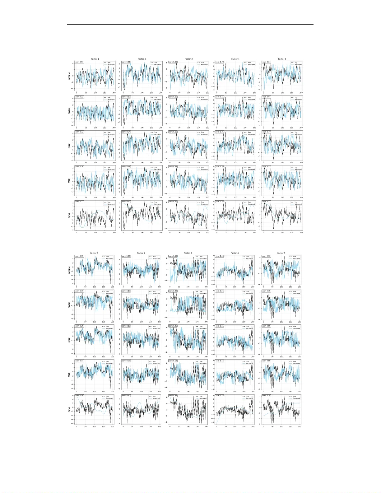
Published as a conference paper at ICLR 2026 C O N D I T I O N A L L Y I D E N T I FI A B L E L A T E N T R E P R E S E N - T A T I O N F O R M U L T I V A R I A T E T I M E S E R I E S W I T H S T R U C T U R A L D Y N A M I C S Minkey Chang Jae Y oung Kim A B S T R AC T W e propose the Identifiable V ariational Dynamic Factor Model (iVDFM), which learns latent factors from multiv ariate time series with identifiability guarantees. By applying iV AE-style conditioning to the innovation pr ocess driving the dy- namics rather than to the latent states, we sho w that factors are identifiable up to permutation and component-wise af fine (or monotone in vertible) transformations. Linear diagonal dynamics preserve this identifiability and admit scalable com- putation via companion-matrix and Krylov methods. W e demonstrate improved factor recov ery on synthetic data, stable intervention accuracy on synthetic SCMs, and competitiv e probabilistic forecasting on real-world benchmarks. 1 I N T RO D U C T I O N Identifying latent temporal dynamics from multiv ariate time series is fundamental in macroeco- nomics, medicine, and causal representation learning (Sch ¨ olkopf et al., 2021). In many applications we seek not just predicti ve accuracy but latent representations that are stable across settings and interpretable as carriers of temporal and causal structure. Follo wing Stock & W atson (2002), we call such v ariables factors ( f t ). Unlike generic latent v ariables z t , factors are not arbitrary: we re- serve the term for latents that admit identifiable and causal interpretations under explicit modeling assumptions. Classical dynamic factor models (DFMs) provide a principled frame work for temporal latent struc- ture but are identifiable only up to orthogonal rotations, so that multiple factorizations induce the same likelihood and recov ered f actors lack a unique semantic or causal reading. Recent identifiable latent-variable models, such as identifiable V AEs (iV AEs), achie ve strong identification in static set- tings by conditioning on auxiliary variables, yet they do not address the temporal structure that is central to factor models. Bridging these lines of work—obtaining f actors that are both dynamic and identifiable—remains an open challenge. W e propose the Identifiable V ariational Dynamic F actor Model (iVDFM) . Our key idea is to achie ve identifiability at the lev el of the inno vation pr ocess that dri ves the dynamics: by applying iV AE-style conditions to the conditional prior on innov ations (conditioned on observed auxiliary variables and a deterministic re gime embedding), we sho w that innov ations are identifiable up to permutation and component-wise affine maps. W e then use linear, diagonal dynamics to map innov ations to factors, which preserves this equi valence class and a voids the rotational ambiguity of classical DFMs while remaining computationally tractable, including support for AR( p ) dynamics in companion form. W e train the model with variational inference and demonstrate improv ed factor recov ery on synthetic dynamic and static factor data, stable intervention accuracy on synthetic structural causal models, and competitiv e probabilistic forecasting on real-world benchmarks. 2 R E L A T E D W O R K 2 . 1 I D E N T I FI C A T I O N P RO B L E M Static representations. Learning compact representations in volves information compression and identification issues. PCA (Pearson, 1901) identifies directions of maximal variance; ICA (Hyv ¨ arinen & Oja, 2000) exploits independence and non-Gaussianity; V AEs (Kingma & W elling, 1 Published as a conference paper at ICLR 2026 2014) extend this to flexible nonlinear latents. In these framew orks, multiple parameterizations can induce the same data distribution, so recov ered latents are not uniquely determined. Recent work restores identifiability via conditioning: iV AEs (Khemakhem et al., 2020) condition the latent prior on observed auxiliary variables and recover latents up to component-wise inv ertible maps in static settings; Concept Bottleneck Models (K oh et al., 2020) enforce identification through human- defined concepts. Our work e xtends the conditioning idea to the dynamic setting by applying it to the innov ation process that drives the latent dynamics. Dynamic r epresentations. Identifiability is harder when latents evolv e over time. Classical DFMs (Stock & W atson, 2002) are identifiable only up to orthogonal transformations ( ˜ z t = Q z t induces the same likelihood for any orthogonal Q ), so recovered factors lack a unique semantic or causal reading. Nonlinear and deep dynamic models face similar issues: without explicit identification, learned trajectories can be rotated or reparameterized without changing the observation distrib ution and thus lack stable interpretations for causal discov ery or intervention analysis. 2 . 2 M O D E L I N G T E M P O R A L D Y NA M I C S V ector autoregressions (V ARs) and Structural V ARs (Sims, 1980; Stock & W atson, 2018) intro- duce identifying assumptions (e.g., via instruments or narrati ve restrictions) to obtain interpretable shocks, but they rely on linearity and scale poorly to high dimensions. Deep forecasters, such as iT ransformer (Liu et al., 2023) and T imeMixer (W ang et al., 2024a), and state-space architectures such as S4 (Gu et al., 2022) and Mamba (Gu & Dao, 2023), offer strong predictiv e performance but either lack stochastic latent factors or yield deterministic embeddings that do not admit a clear factor interpretation. Deep Dynamic Factor Models (Andreini et al., 2020) and Deep Kalman Filters (Krishnan et al., 2015) combine probabilistic temporal structure with flexible nonlinear mappings, yet they do not provide identifiability guarantees, so that the learned factors remain defined only up to equiv alence classes that can include rotations. Our model retains explicit stochastic dynamics and a factor structure while achie ving identifiability at the innovation le vel. 2 . 3 C A U S A L I N F E R E N C E Causal inference aims to recover cause–effect structure and to reason under interventions (Pearl, 2009; Peters et al., 2017). In many settings, observed v ariables are mixtures of latent causal f actors; without identifying those factors, causal conclusions are ambiguous (Sch ¨ olkopf et al., 2021; Spirtes et al., 2000). In time series, rotations or reparameterizations of the latent space yield observationally equiv alent but causally distinct interpretations, so that identifiability is a prerequisite for reliable causal discov ery and intervention analysis. Structural V ARs (Blanchard & Quah, 1989) address identification via instruments or narrati ve restrictions but rely on domain-specific assumptions and linearity . For learned factors to support causal applications in a general setting, the y must be identi- fiable. W e pro vide identifiability at the innovation lev el (Section 3) so that recovered factors admit a well-defined causal interpretation and can be used meaningfully in intervention e xperiments. 3 I D E N T I FI A B L E V A R I A T I O N A L D Y N A M I C F AC T O R M O D E L W e propose the Identifiable V ariational Dynamic F actor Model (iVDFM) : a framew ork that marries identifiable latent-variable modeling with explicit stochastic dynamics. The key idea is to achiev e identifiability at the lev el of the innovation process that driv es the dynamics, then let the dynamics propagate this structure to the latent factors. W e first define the innov ation and the conditions under which it is identifiable; we then specify the dynamics that map innov ations to factors; and we finally describe how we estimate the model and train it. 3 . 1 I N N OV A T I O N The source of uncertainty in the model is the innovation η t ∈ R r at each time step. W e take it to follow a conditional e xponential-family distrib ution that factors across components and depends on an observed auxiliary variable u t (e.g., time index or e xogenous co v ariates) and a regime embedding e t . This dependence on u t and e t is what allows the prior to v ary across time or context, which is 2 Published as a conference paper at ICLR 2026 necessary for identifiability . Concretely , p ( η t | u t , e t ) = r Y i =1 h i ( η i,t ) exp  T i ( η i,t ) ⊤ λ i ( u t , e t ) − A i ( λ i ( u t , e t ))  , (1) where for the i th component, T i and λ i ( u t , e t ) are the suf ficient statistics and natural parameters, h i is the base measure, and A i is the log-partition function. The regime embedding is defined as e t = P K k =1 π t,k e k with π t = softmax(RegimeNet( u t )) and learnable vectors e k ∈ R d per regime; K = 1 corresponds to a single fixed embedding. Crucially , we condition on this expected embedding rather than a sampled regime, so e t is deterministic given u t . This choice preserves identifiability and keeps the recurrence dif ferentiable (Appendix A). When K > 1 , the prior is the mixture p ( η t | u t , e t ) = P K k =1 π t,k p k ( η | u t ) with λ k ( u t ) = h ( u t , e k ) . Under these assumptions, conditioning on u t and e t yields identification up to permutation and component-wise affine transformations (Hyv ¨ arinen & Oja, 2000; Khemakhem et al., 2020). In- tuitiv ely , the sufficient statistics form a basis for each component’ s log-density; if the natural pa- rameters λ ( u , e ) v ary suf ficiently across at least r + 1 distinct values of ( u , e ) so that they span a full-rank subspace, then the innov ation components are identifiable. In other words, the auxiliary variable and regime embedding must induce enough variation in the natural parameters across time or context so that the model can tell the components apart. Gaussian innovations are degenerate for identifiability (Appendix B); we therefore use non-Gaussian exponential-family innovations (e.g. Laplace) in practice. 3 . 2 D Y N A M I C S The latent factors f t ∈ R r ev olve according to the innov ations. W e take the dynamics to be linear and diagonal: f t +1 = ¯ A t f t + ¯ B t η t , (2) with ¯ A t , ¯ B t ∈ R r × r diagonal. When K > 1 , we set ¯ A t = P k π t,k A k and ¯ B t = P k π t,k B k , and we freeze π t per windo w so that the dynamics are constant within each window . The diagonal structure is important: each factor ev olves from its o wn lagged values and its own innov ation component only , with no cross-factor mixing. As a result, the component-wise structure inherited from the inno vation prior is preserved, and identifiability can propagate from innov ations to factors without introducing rotational ambiguity . T o capture higher-order temporal dependence we use AR( p ) in companion form. The current and p − 1 lagged factor vectors are stacked into an augmented state s t ∈ R rp that obeys first-order Markov dynamics s t +1 = A s t + B η t with block-diagonal A , B (companion blocks per factor (Zhang et al., 2023)). The factors are then a con volution of past innov ations, f t = P t − 1 j =0 H j η t − 1 − j , where H j is the impulse response at lag j ; this form allo ws ef ficient FFT - or Krylov-based ev aluation for long horizons. Formal definitions and the full unrolling are giv en in Appendix A. Stochastic- ity enters only through the innov ations; the map from innov ations to factors is deterministic and time-in variant. Because it is component-wise and introduces no rotations or cross-factor mixing, the equiv alence class (permutation and component-wise affine maps) carries over unchanged to the factors. Theorem A.2 in Appendix A giv es the formal statement and proof. 3 . 3 E S T I M A T I O N Let y t ∈ R N denote the observed multi variate time series. W e assume an observation model y t = g ( f t ) + ε t , ε t ∼ p ε , (3) where g : R r → R N is an injectiv e decoder and p ε is observation noise with full support. The decoder maps the latent factors to observations; injectivity ensures that distinct f actors yield distinct observation distrib utions, which is required for identifiability . In this setup the only stochastic latent variables are the innov ations { η t } ; the factors { f t } are deter- ministic functions of past innov ations via the linear dynamics (Appendix A.2). The posterior over innov ations given observations is therefore proportional to the product of the innovation priors and the likelihoods of the observations gi ven the implied factors. This posterior is intractable: the prod- uct over time and the nonlinear decoder preclude closed-form inference, so we approximate it with 3 Published as a conference paper at ICLR 2026 Algorithm 1 Estimation of identifiable AR( p ) factors from innov ations (iVDFM) Require: Observations y 1: T , auxiliary u 1: T , regime embeddings e 1: T (from u 1: T ), initial state f 0 ∈ R r (or s 0 ∈ R rp for AR( p )), encoder ϕ , decoder and dynamics θ . Ensure: θ , ϕ maximizing the ELBO. 1. Compute e t from u t ; encode ( y 1: T , u t , e t ) 7→ ( µ t , σ t ) for t = 1 , . . . , T . 2. Sample η t = µ t + σ t ⊙ ϵ t , ϵ t ∼ N ( 0 , I ) . 3. Reconstruct f t +1 = ¯ A t f t + ¯ B t η t (or companion form); f t = H ( η 1: t ) . 4. Decode ˆ y t = g ( f t ) ; compute log p θ ( y t | f t ) . 5. Compute ELBO (Eq. 4), backprop, update θ , ϕ . variational inference. W e tak e the variational posterior to factorize across time and components. The encoder ϕ maps ( y 1: T , u t , e t ) to the parameters of a Gaussian q ϕ ( η t | · ) = N ( µ ϕ ( t ) , diag ( σ 2 ϕ ( t ))) . Identifiability is a property of the generative prior; the variational posterior may use the full obser- vation sequence without weakening that result. W e use the reparameterization trick (Kingma & W elling, 2014) so that gradients with respect to ϕ flow through samples: η t = µ ϕ ( t ) + σ ϕ ( t ) ⊙ ϵ t with ϵ t ∼ N ( 0 , I ) . The factors then follow from the dynamics. W e learn the parameters θ (decoder, prior including { e k } and RegimeNet, dynamics) and ϕ (en- coder) by maximizing the evidence lower bound (ELBO). Because the factors are deterministic functions of the innov ations, the joint likelihood factorizes over time into the observation likeli- hoods and the innov ation priors. The ELBO is L = E q ϕ ( η 1: T | y 1: T , u 1: T , e 1: T ) " T X t =1 log p θ ( y t | f t ( η 1: t )) # − T X t =1 KL( q ϕ ( η t | y 1: T , u t , e t ) ∥ p θ ( η t | u t , e t )) , (4) with f t +1 = ¯ A t f t + ¯ B t η t and f 0 giv en. The first term is the expected reconstruction log-likelihood: it measures how well the model fits the observations given the inferred innov ations and dynamics. The second term is the sum of KL div ergences between the variational posterior and the innovation prior at each time step; it regularizes the posterior toward the prior . Maximizing this objecti ve trains the model while preserving the identifiability guarantees of Theorem A.2. 4 E X P E R I M E N T S W e ev aluate iVDFM in three experiments: (1) factor recovery on synthetic data with known la- tent factors; (2) causal intervention on synthetic time series from a known structural causal model (SCM); and (3) probabilistic forecasting on real-world data. They address representation quality , intervenability , and downstream forecast performance. 4 . 1 F AC T O R R E C OV E RY W e use synthetic data-generating processes (DGPs) with known latent factors in two settings: a dy- namic setting (AR dynamics driven by inno vations) and a static setting (latent variables conditional on an auxiliary , no temporal dependence). Observ ations are obtained via a nonlinear mixing. W e compare recov ered factors to ground truth using permutation-inv ariant matching (max-weight cor- relation alignment) and report MCC (higher better), subspace distance (lower better), smoothness (lower better), and T race R 2 (higher better). DGP details, metric definitions, and baselines are in Appendix C. W e compare iVDFM to DFM, DDFM, V AE, and iV AE. T able 1 summarizes the results. 4 Published as a conference paper at ICLR 2026 T able 2: Causal intervention on synthetic SCMs (iVDFM). IRF-MSE, IRF-MAE: mean squared / absolute error between ground-truth and model-implied impulse response; Sign Acc: fraction of (time step, v ariable) pairs with correct sign; IRF Corr: Pearson correlation with ground truth. Mean ± std over fi ve simulations. SCM IRF-MSE ↓ IRF-MAE ↓ Sign Acc ↑ IRF Corr ↑ Base (linear) 0 . 89 ± 1 . 01 0 . 45 ± 0 . 23 0 . 58 ± 0 . 25 0 . 21 ± 0 . 75 Regime 1 . 28 ± 0 . 92 0 . 77 ± 0 . 27 0 . 60 ± 0 . 27 0 . 13 ± 0 . 62 Chain 2 . 18 ± 2 . 40 0 . 97 ± 0 . 40 0 . 58 ± 0 . 33 0 . 20 ± 0 . 62 T able 1: Factor recovery on synthetic data ( T =200 , N =20 , r =5 ): dynamic vs. static DGP . Metrics after MCC-based matching where applicable. Higher is better for MCC and trace R 2 ; lower for subspace distance and smoothness. Model MCC ↑ Subspace ↓ Smoothness ↓ T race R 2 ↑ Dynamic Static Dynamic Static Dynamic Static Dynamic Static iVDFM 0.6876 0.5554 0.3456 0.7163 1.7543 1.7923 0.8664 0.5955 DDFM 0.5482 0.5989 0.7632 0.6147 1.9848 2.3296 0.5523 0.6745 iV AE 0.6439 0.5678 0.4123 0.5055 1.6783 2.2504 0.8316 0.7766 V AE 0.6474 0.6405 0.4105 0.4520 1.6760 2.3255 0.8275 0.8078 DFM 0.3173 0.3665 1.0276 1.0319 0.1195 0.1257 0.2894 0.3068 On the dynamic DGP , iVDFM leads on MCC, subspace distance, and Trace R 2 ; V AE and iV AE are second on MCC and Trace R 2 . On the static DGP , V AE leads on MCC, subspace distance, and Trace R 2 ; DDFM and iV AE are second on MCC and Trace R 2 respectiv ely . DFM has the weakest MCC and Trace R 2 in both settings, in line with the rotational indeterminacy of Gaussian factor models. DFM and DDFM attain the best smoothness (lowest step-to-step variation) in both settings; this is likely due to the models’ nature: both use linear (or linear-in-factor) dynamics in the latent space (Stock & W atson, 2002; Andreini et al., 2020), so the recovered factor path has small increments by construction rather than from superior alignment. Thus smoothness reflects the dynamical prior (linear vs. flexible) rather than identifiability per se. Experiment (2) below focuses on intervenability . Hyperparameter sensitivity and visualizations are in Appendix C and D. 4 . 2 C A U S A L I N T E RV E N T I O N Factor recovery assesses alignment up to the same equiv alence class as in Section 3; it does not show whether the representation supports interventions. W e therefore run a controlled intervention experiment on synthetic series from a kno wn SCM: exogenous innovations driv e states and obser- vations, and we compare the model-implied impulse response to ground truth after applying the do-operator at the representation lev el. Metrics are IRF-MSE and sign accuracy (details and scope in Appendix C). On all three SCM variants (base linear , regime, chain), iVDFM achiev ed bounded IRF error and stable sign accuracy (T able 2). Sign accuracy remained consistent ev en under the more complex regime and chain SCMs, indicating that the learned representation is intervenable across different causal structures. W ith experiment (1), this supports that identifiable dynamics yield interpretable, intervenable factors rather than merely good fit. 4 . 3 P R O B A B I L I S T I C F O R E C A S T I N G W e ev aluate probabilistic forecasts on fiv e real-world datasets (ETTh1, ETTh2, ETTm1, ETTm2, W eather) at horizons 96, 192, 336, and 720. W e report CRPS and MSE on standardized data, av eraged over horizons per dataset. T able 3 summarizes the results. iVDFM is competitiv e on probabilistic forecasting across datasets: it attains CRPS and MSE (std.) in the same range as dedicated forecasting baselines (T imeMixer , TimeXer , DDFM). T imeMixer 5 Published as a conference paper at ICLR 2026 T able 3: CRPS and MSE (standardized), av eraged over horizons. Ro ws: dataset; columns: per- model CRPS and MSE (std.). Dataset iVDFM iT ransformer T imeMixer T imeXer DDFM CRPS MSE (std.) CRPS MSE (std.) CRPS MSE (std.) CRPS MSE (std.) CRPS MSE (std.) ETTh1 0.2822 1.2579 0.6927 1.2959 0.2761 0.8010 0.5423 1.1891 0.3340 1.3415 ETTh2 0.2681 1.0164 0.5014 1.0175 0.2304 0.4014 0.4519 0.9902 0.2775 1.0125 ETTm1 0.3151 1.2206 0.7055 1.2879 0.2292 0.5468 0.5978 1.2503 0.3563 1.2773 ETTm2 0.3397 1.0982 0.6439 1.3300 0.2323 0.4342 0.5310 1.3949 0.4595 2.3075 W eather 0.2710 1.1837 0.3157 0.7026 0.1633 0.3406 0.2808 0.7072 0.1642 0.4393 leads on ETTh2, ETTm1, ETTm2 and W eather on a verage; DDFM is strong on W eather . The strong probabilistic performance of T imeMixer and iVDFM may reflect their structural inductiv e biases: T imeMixer’ s decomposable multiscale mixing (W ang et al., 2024a) separates and recombines past segments at multiple scales, which can help capture uncertainty at dif ferent horizons; iVDFM mod- els uncertainty e xplicitly at the inno vation lev el and propagates it through factor dynamics, yielding a proper generati ve predicti ve distrib ution. iVDFM does not dominate point or probabilistic metrics here, consistent with its primary design for identifiable dynamics and intervenability rather than raw forecast accuracy . The results show that the learned representation remains useful for downstream forecasting while retaining the interpretability and causal structure exploited in experiments (1) and (2). 5 C O N C L U S I O N In this w ork we e xtended the v ariational framework with conditionally identifiable latent representa- tion to the dynamic setting. By applying iV AE-style identifiability to the innovation process (rather than latent states) and using linear diagonal dynamics, we obtain a model that, despite its restricti ve structure, can be trained on multiv ariate time series and yields representations that are identified up to the usual equiv alence class and support interpretable, intervenable factors. This addresses rota- tional indeterminacy of classical dynamic factor models while admitting scalable computation via companion matrix and Krylov methods. In experiments, we found that on DGPs with dynamic structure, iVDFM showed stronger perfor- mance and recovered factors at a high level. For causal intervention, we observed a consistent pattern of sign identification across SCM v ariants—including under misspecification and regime-integrated DGPs—which indicates robust intervenability of the learned representation. For probabilistic fore- casting, although recent SO T A models excel at point-wise prediction, iVDFM remained competiti ve in the probabilistic setting, demonstrating that the identifiable representation is useful for down- stream forecasting while retaining structural interpretability . Further research may e xplore other conditional contexts (e.g., learned or task-specific embeddings), relax the dynamical or prior structure while preserving identifiability , and extend the approach to other modalities such as language or image sequences. A C K N O W L E D G M E N T S The author is grateful to Professor Jae Y oung Kim for insightful comments and guidance during the dev elopment of this work. R E F E R E N C E S Paolo Andreini, Cosimo Izzo, and Giov anni Ricco. Deep dynamic factor models. arXiv preprint arXiv:2007.11887 , 2020. Olivier J. Blanchard and Dann y Quah. The dynamic ef fects of aggre gate demand and supply distur- bances. American Economic Review , 79(4):655–673, 1989. Albert Gu and Tri Dao. Mamba: Linear-time sequence modeling with selectiv e state spaces. arXiv pr eprint arXiv:2312.00752 , 2023. 6 Published as a conference paper at ICLR 2026 Albert Gu, Karan Goel, and Christopher R ´ e. Efficiently modeling long sequences with structured state spaces. arXiv preprint , 2022. Aapo Hyv ¨ arinen and Erkki Oja. Independent component analysis: Algorithms and applications. Neural Networks , 13(4–5):411–430, 2000. Ilyes Khemakhem, Diederik Kingma, Riccardo Monti, and Aapo Hyv ¨ arinen. V ariational autoen- coders and nonlinear ica: A unifying frame work. In Pr oceedings of the 23r d International Confer ence on Artificial Intelligence and Statistics , volume 108, pp. 2207–2217, 2020. URL https://proceedings.mlr.press/v108/khemakhem20a.html . Diederik P . Kingma and Max W elling. Auto-encoding variational bayes. In International Conference on Learning Repr esentations , 2014. Pang W ei K oh, Thao Nguyen, Y ew Siang T ang, Stephen Mussmann, Emma Pierson, Been Kim, and Perc y Liang. Concept bottleneck models. In International Confer ence on Machine Learning , 2020. Rahul G. Krishnan, Uri Shalit, and David A. Sontag. Deep kalman filters. arXiv preprint arXiv:1511.05121 , 2015. Y ong Liu, T engge Hu, Haoran Zhang, Haixu W u, Shiyu W ang, Lintao Ma, and Mingsheng Long. itransformer: In verted transformers are effecti ve for time series forecasting. arXiv pr eprint arXiv:2310.06625 , 2023. Judea Pearl. Causality: Models, Reasoning , and Inference . Cambridge Uni versity Press, Cambridge, UK, 2nd edition, 2009. Karl Pearson. On lines and planes of closest fit to systems of points in space. Philosophical Maga- zine , 2(11):559–572, 1901. Jonas Peters, Dominik Janzing, and Bernhard Sch ¨ olkopf. Elements of Causal Inference: F ounda- tions and Learning Algorithms . MIT Press, Cambridge, MA, 2017. Bernhard Sch ¨ olkopf, Dominik Janzing, Jonas Peters, Sebastian Bauer, Kun Xu, Patrick Bl ¨ obaum, Kun Zhang, and Joris Mooij. T oward causal representation learning. Pr oceedings of the National Academy of Sciences , 118(23):e2021297118, 2021. Christopher A. Sims. Macroeconomics and reality . Econometrica , 48(1):1–48, 1980. Peter Spirtes, Clark Glymour , and Richard Scheines. Causation, Pr ediction, and Searc h . MIT Press, Cambridge, MA, 2nd edition, 2000. James H. Stock and Mark W . W atson. Forecasting using principal components from a large number of predictors. Journal of the American Statistical Association , 97(460):1167–1179, 2002. James H. Stock and Mark W . W atson. Identification and estimation of dynamic causal effects in macroeconomics using external instruments. The Economic Journal , 128(610):917–948, 2018. Shiyu W ang, Haixu W u, Xiaoming Shi, T engge Hu, Huakun Luo, Lintao Ma, James Y . Zhang, and Jun Zhou. T imemixer: Decomposable multiscale mixing for time series forecasting. arXiv pr eprint arXiv:2405.14616 , 2024a. Y uxuan W ang, Haixu W u, Jiaxiang Zhang, Zhiyu Gao, Jianmin W ang, Mingsheng Long, and Jian y- ong W ang. T imexer: Empowering transformers for time series forecasting with exogenous vari- ables. Advances in Neural Information Pr ocessing Systems , 37, 2024b. Qiang Zhang, Y ifei Y an, Y u Fan, Xiyuan W ang, Xinshang Chen, Hao Sun, and Thomas S. Huang. Spacetime: A unified framework for learning in time series and beyond. arXiv pr eprint arXiv:2301.04833 , 2023. 7 Published as a conference paper at ICLR 2026 A I D E N T I FI A B I L I T Y P R O O F This appendix gives a self-contained formalization of the identifiability argument in Section 3. Un- der iV AE-style conditions (Khemakhem et al., 2020) on the innovation prior conditioned on aux- iliary and regime, innovations are identifiable up to permutation and component-wise affine maps; diagonal (or block-diagonal companion) dynamics then propagate this equiv alence class to the la- tent factors without rotational ambiguity , in contrast to classical Gaussian DFMs (Stock & W atson, 2002). A . 1 S E T U P A N D N O TA T I O N The generativ e model includes regime from the start: • Innovations: η t ∈ R r with conditional prior p ( η t | u t , e t ) in exponential-family form (Eq. 1), where the auxiliary u t is observed and the regime embedding e t = P K k =1 π t,k e k is a deterministic function of u t via π t = softmax(RegimeNet( u t )) ; K = 1 is the single- regime case. • Dynamics: f t +1 = ¯ A t f t + ¯ B t η t with diagonal ¯ A t = P k π t,k A k , ¯ B t = P k π t,k B k (or companion-form s t +1 = A s t + B η t , f t = C s t with block-diagonal A , B ). No stochastic regime sampling: π t is fixed giv en u t , so the recurrence is deterministic and component- wise. • Observations: y t = g ( f t ) + ε t , ε t ∼ N ( 0 , σ 2 I N ) , with g injective and σ 2 fixed. Definition A.1 (Identifiability up to a class) . Innovations (or factors) ar e identifiable up to a class of transformations T if, for any two parameterizations that induce the same p ( y 1: T , u 1: T ) , the corr esponding latent variables are r elated by a transformation in T almost surely . A . 2 C O M PA N I O N F O R M ( A R ( p ) ) For AR( p ) we stack the current and p − 1 lagged factor vectors into s t = ( f ⊤ t , f ⊤ t − 1 , . . . , f ⊤ t − p +1 ) ⊤ ∈ R rp , which obeys s t +1 = A s t + B η t with block-diagonal A , B . Unrolling gives s t = A t s 0 + P t − 1 j =0 A j B η t − 1 − j . W ith C such that f t = C s t , the factors are f t = C A t s 0 + P t − 1 j =0 H j η t − 1 − j where H j := C A j B is the impulse response at lag j . This allows efficient FFT - or Krylov-based ev aluation for long horizons (Zhang et al., 2023). A . 3 M A I N R E S U L T Theorem A.2 (Identifiability of dynamic f actors) . Under the gener ative model above, assume: 1. The innovation prior p ( η t | u t , e t ) is conditional exponential-family with linearly inde- pendent sufficient statistics (component-wise pr oduct form). The natural-parameter map λ ( u , e ) has full column rank for at least r + 1 distinct values of ( u , e ) (or a set spanning a full-rank subspace). Her e e is the r e gime embedding, deterministic given u . 2. π t depends only on u t ; dynamics use expected matrices ¯ A t , ¯ B t with diagonal A k , B k per r egime . 3. The decoder g is injective on the support of f t . 4. Observation noise has full support, admits deconvolution, and σ 2 is fixed (not learnable). 5. Base measur es have full support, r ≤ N , and all mappings ar e measur able and inte grable. Then the innovations { η t } T t =1 ar e identifiable fr om ( y 1: T , u 1: T ) up to T (Definition A.1, with T the class of permutation and component-wise affine maps; or monotone in vertible under additional r egularity). The latent factor trajectories { f t } T t =1 and the associated dynamic parameters ar e iden- tifiable up to the same class. 8 Published as a conference paper at ICLR 2026 Proof sketch. T wo parameterizations that yield the same p ( y 1: T , u 1: T ) must agree on the marginal ov er ( η t , u t , e t ) ; the iV AE argument (Khemakhem et al., 2020) then pins innov ations up to T . Diag- onal dynamics preserv e this class on f actors; injecti vity of g and fixed σ 2 prev ent further ambiguity . A . 4 P R O O F O F T H E O R E M A . 2 Pr oof. Let ( θ , η , f ) and ( ˜ θ , ˜ η , ˜ f ) be tw o parameterizations that induce the same p ( y 1: T , u 1: T ) . W e show the y differ only by a transformation in T . Step 1 (Innov ations). The conditioning variable ( u t , e t ) is deterministic giv en u t and observed, so it is a valid auxiliary for iV AE. The prior has the form p ( η t | u t , e t ) = r Y i =1 h i ( η i,t ) exp  T i ( η i,t ) ⊤ λ i ( u t , e t ) − A i ( λ i ( u t , e t ))  . (5) By Khemakhem et al. (2020), any alternativ e parameterization that yields the same joint distribu- tion of ( y t , u t ) (hence the same marginal over ( η t , u t , e t ) ) satisfies ˜ η i,t = h i ( η π ( i ) ,t ) a.s. for some permutation π and component-wise affine maps { h i } (or monotone inv ertible under additional reg- ularity). The full-rank condition on λ ( u , e ) ensures the class is no larger; thus innov ations are identifiable up to T . Step 2 (Propagation to factors). W ith diagonal ¯ A t , ¯ B t (or block-diagonal companion A , B ), the dynamics are linear and component-wise: f t = H t ( η 1: t ) with no cross-dimension mixing. From Step 1, ˜ η t = h ( η π ,t ) . Applying the same component-wise map yields ˜ f i,t = h i ( f π ( i ) ,t ) a.s. So T is preserved on factors; the dynamics introduce no rotational or linear mixing. Step 3 (Observation model). For the same p ( y t | u t ) , the conditional mean g ( f t ) is determined by the distribution of f t | u t . From Step 2, ˜ f t = h ( f π ,t ) . Injectivity of g and the component-wise structure of h imply the decoder is determined up to T . Fixed σ 2 prev ents matching the observation distribution by rescaling noise and preserv es identifiability . A . 5 R E M A R K S Identifiability is established at the innovation lev el via variation of λ with ( u , e ) , then inherited by { f t } through deterministic, component-wise dynamics. Companion-form and Krylov implementa- tions are for computation only; H t need not be in vertible. Under v ariational inference, identifiability is a property of the generative model; the variational posterior may depend on the full observation sequence without changing the result. What breaks identifiability . (i) Conditioning on a continuous latent z t (e.g. η t ∼ p ( η | u t , z t ) ) breaks the iV AE argument because the conditioning variable is no longer fixed. (ii) Feeding data or attention into the innov ation (e.g. η t = µ ( u t , y t − L : t ) + . . . ) makes the auxiliary non-e xogenous and identifiability is lost. Encoder . The v ariational encoder may depend on e t ; identifiability is a property of the generativ e model, and the posterior may use the full sequence. B D E G E N E R AC Y O F G AU S S I A N I N N OV A T I O N S B . 1 O V E RV I E W This appendix explains why the inno vation process { η t } cannot be identified when it is Gaus- sian, even with auxiliary variables and temporal dynamics (Hyv ¨ arinen & Oja, 2000; Khemakhem et al., 2020). That degeneracy motiv ates the use of non-Gaussian exponential-family innovations in iVDFM (Section 3). W e present the argument for the single-re gime case ( K = 1 ): the regime embedding e t is then fixed, so conditioning on it is implicit and we write the prior as p ( η t | u t ) . The same degeneracy holds for K > 1 when conditioning on both u t and e t ; the Gaussian fam- ily remains closed under linear maps regardless of how the conditional parameters depend on the 9 Published as a conference paper at ICLR 2026 embedding. This appendix is distinct from the “constant context” degeneracy in the ablation (Ap- pendix E), where u t ≡ u 0 remov es variation in the prior; here we assume u t varies b ut the innov ation family is Gaussian. B . 2 S E T U P : G AU S S I A N I N N O V A T I O N S I N E X P O N E N T I A L - FA M I L Y F O R M Suppose innov ations are conditionally Gaussian, η t | u t ∼ N ( µ ( u t ) , Σ( u t )) , (6) with Σ( u t ) full rank. The log-density is log p ( η t | u t ) = − 1 2 η ⊤ t Σ( u t ) − 1 η t + η ⊤ t Σ( u t ) − 1 µ ( u t ) + c ( u t ) , (7) where c ( u t ) does not depend on η t . In exponential-family form, the sufficient statistics are T ( η t ) = ( η t , vec( η t η ⊤ t )) and the natural parameters λ ( u t ) are functions of Σ( u t ) − 1 and Σ( u t ) − 1 µ ( u t ) . The log-density therefore lies in the span of at most r + r ( r + 1) / 2 basis functions (linear and quadratic in η t ). Crucially , this span is invariant under in vertible linear maps : for any R ∈ R r × r in vertible, η t 7→ R η t preserves the quadratic form, so the likelihood cannot distinguish η t from ˜ η t = R η t . B . 3 M A I N R E S U L T : G AU S S I A N I N N OV ATI O N S A R E N OT I D E N T I FI A B L E The identifiability result of Khemakhem et al. (2020) requires the natural-parameter map λ ( u ) to span a full-rank subspace over distinct u , so that observing multiple u pins down the innovation components. In the Gaussian case the equiv alence class of parameters giving the same observation distribution is too lar ge: any in vertible linear reparameterization preserves the Gaussian family . Proposition B.1 (Gaussian innovations are not identifiable) . Let η t | u t ∼ N ( µ ( u t ) , Σ( u t )) with Σ( u t ) full rank. F or any invertible R ∈ R r × r , the transformed innovations ˜ η t = R η t ar e also Gaussian, ˜ η t | u t ∼ N  R µ ( u t ) , R Σ( u t ) R ⊤  , (8) and the likelihood p ( y 1: T | u 1: T ) is unchanged. Thus innovations are identifiable at most up to in vertible linear transformation, not up to permutation and component-wise affine maps as in the non-Gaussian case (Appendix A). Even when µ ( u t ) or Σ( u t ) depend on u t , the variation stays within the same quadratic family , so the auxiliary variable cannot break rotational or scaling symmetry . Example ( r = 2 ). For η t | u t ∼ N ( 0 , Σ( u t )) , any orthogonal Q gives ˜ η t = Q η t ∼ N ( 0 , Q Σ( u t ) Q ⊤ ) ; the observation distribution is unchanged, so the model cannot distinguish the original from the rotated innov ations. B . 4 I M P L I C A T I O N S F O R DY NA M I C FA C T O R M O D E L S In classical Gaussian dynamic factor models (Stock & W atson, 2002), factors e volve as f t +1 = A f t + η t , η t ∼ N ( 0 , Σ) , (9) with a linear decoder . The joint distribution of observations is then in variant under f t 7→ R f t , A 7→ RAR − 1 , Σ 7→ R Σ R ⊤ for any in vertible R —the well-known rotational indeterminacy . T emporal dependence or higher -order (e.g. companion-form) dynamics do not remov e this ambiguity , because linear Gaussian dynamics remain closed under linear maps. Restricting A to be diagonal av oids cross-factor mixing in the dynamics but does not restore identi- fiability . The equiv alence class is fixed at the innovation lev el: any in vertible ˜ η t = R η t preserves the Gaussian family and can be paired with a transformed decoder and dynamics to yield the same observations. Diagonal A only constrains how factors e volv e over time, not the inv ariance of the innov ation distribution under linear mixing. 10 Published as a conference paper at ICLR 2026 B . 5 C O N T R A S T W I T H N O N - G AU S S I A N I N N O V A T I O N S A N D TA K E AW AY For a non-Gaussian exponential family with linearly independent sufficient statistics (e.g. Laplace, Student- t ), the log-density is not in variant under general linear mixing (Hyv ¨ arinen & Oja, 2000): ˜ η t = R η t leav es the product form only when R is a permutation of a scaled identity (permutation and component-wise scaling). Conditioning on u t then yields variation in natural parameters that spans a full-rank subspace, so the iV AE conditions of Khemakhem et al. (2020) hold and innov a- tions are identifiable up to permutation and component-wise affine (or monotone in vertible under regularity). iVDFM uses such non-Gaussian innov ation priors (e.g. Laplace) so that identifiability is achiev ed at the innovation le vel and propagated by the dynamics (Theorem A.2). The degeneracy of Gaussian innov ations is thus a property of the Gaussian family , not of the dynamic structure. iVDFM avoids it by using conditional non-Gaussian inno vations. C E X P E R I M E N T D E TA I L S This appendix gives details for the experiments in Section 4: factor recovery , causal intervention, and probabilistic forecasting. C . 1 F AC T O R R E C OV E RY Synthetic DGPs. W e use two synthetic DGPs adapted from Khemakhem et al. (2020) and An- dreini et al. (2020). Static setting: latents are generated independently across time conditional on an auxiliary variable, with observations via a nonlinear mixing; T = 200 , N = 20 , r = 5 . Dynamic setting: latent factors follow AR dynamics driven by stochastic innovations, with observations via a nonlinear decoder; same T , N , r . This isolates the role of temporal dynamics while keeping measurement comparable. Baselines. iVDFM is compared to: DFM (Stock & W atson, 2002) (linear dynamic factor model, identifiable only up to orthogonal rotations); DDFM (Andreini et al., 2020) (nonlinear measurement, no identifiability guarantees); V AE (Kingma & W elling, 2014) (no auxiliary conditioning); iV AE (Khemakhem et al., 2020) (identifiable V AE applied per time step with time as auxiliary , ignoring temporal dependence). Metrics. Let F ∈ R T × r be ground-truth factors and ˆ F ∈ R T × r recov ered factors. MCC (higher better): max-weight assignment over Pearson correlations between standardized columns of F and ˆ F ; MCC = 1 r max π ∈ S r P r i =1 | C i,π ( i ) | . Subspace distance (lower better): principal angle distance between column spans; with orthonormal bases Q F , Q ˆ F and singular values σ i of Q ⊤ F Q ˆ F (clamped to [0 , 1] ), Subspace = 1 r P r i =1 arccos( σ i ) . Smoothness (lower better): av erage ℓ 2 step size of the recovered trajectory; DFM and DDFM attain low values by construction due to linear latent dynamics (Stock & W atson, 2002; Andreini et al., 2020). Trace R 2 (higher better): fraction of true factor v ariance explained by the recovered span (Andreini et al., 2020); range [0 , 1] . Protocol. W e run N sim = 10 simulations per suite (dynamic and static) with fixed seeds so all models see the same data; we report mean and std of each metric. Common settings: window = 200 , max epochs = 200 , learning rate = 0 . 002 . iVDFM hyperparameters are tuned on the dynamic suite only (Optuna maximizing mean MCC ov er the same 10 seeds); the best configuration is used in both suites. Results: T able 1. C . 2 C A U S A L I N T E RV E N T I O N SCM. W e use a minimal time-series SCM (Pearl, 2009) with exogenous innov ations as the only source of randomness. State ev olution: f t = A f t − 1 + ϵ t , f 0 = 0 , with A ∈ R r × r stable. Obser- vation map: y t = C f t (base/linear) or y t = g ( f t ) (general). Shocks ϵ t are i.i.d. non-Gaussian (e.g. Laplace), giving the causal graph ϵ t → f t → y t . 11 Published as a conference paper at ICLR 2026 Do-intervention and IRF . An intervention at ( t 0 , k ) sets ϵ ( k ) t 0 = c and leav es other ϵ unchanged. The impulse response function (IRF) at horizon h is the difference in expected observ ations at t 0 + h under intervention vs. no intervention. Under the SCM with linear C , the ground-truth IRF is IRF true ( h ) = c · C A h e k ∈ R N . Base SCM: A = ρI ; regime SCM: A regime-dependent; chain SCM: A upper triangular (factor i influences i + 1 ). Model-implied IRF (iVDFM). iVDFM learns an innov ation process η t and dynamics f t = F ( η 1: t ) , y t = g θ ( f t ) . Under the main-text identifiability conditions, η t aligns with the SCM’ s ϵ t up to the same equiv alence class (Appendix A). W e define the model-implied IRF by: (1) fitting on observational data; (2) constructing η do by setting ( η do t 0 ) ( k ) = c ; (3) propagating through learned dynamics to get f do ; (4) decoding baseline b y t and intervention y do t ; (5) d IRF( h ) = y do t 0 + h − b y t 0 + h . This ev aluation is defined only for iVDFM. Metrics and protocol. W e compare d IRF to IRF true ov er horizon × variables. IRF-MSE (lower better): mean squared error over the grid. Sign accuracy (higher better): fraction of ( h, n ) pairs with sign( d IRF h,n ) = sign(IRF true ,h,n ) . W e also report IRF-MAE and Pearson correlation (Ap- pendix T able 4). W e generate series from three SCM variants (base, re gime, chain), train iVDFM on observational data only , tune with Optuna (minimize IRF-MSE; structural parameters fixed). Fi ve simulations per setting. Results: T able 2 (main text); T able 4 (stress tests). All experiments on a single GPU. C . 3 P R O B A B I L I S T I C F O R E C A S T I N G Datasets and task. W e use fiv e real-world multiv ariate time-series datasets: ETTh1 and ETTh2 (electricity transformer temperature, hourly), ETTm1 and ETTm2 (15-minute), and W eather . For each dataset we train on a fixed train/val split and ev aluate out-of-sample forecasts at horizons H ∈ { 96 , 192 , 336 , 720 } . Predictions are made in standardized (scaled) space: we fit a scaler on the training set and ev aluate metrics without in verse-transforming, so that MSE and CRPS are comparable across variables and datasets. Baselines. iVDFM is compared to: iTransformer (Liu et al., 2023), TimeMix er (W ang et al., 2024a), TimeXer (W ang et al., 2024b), DDFM (Andreini et al., 2020), and MLPMulti variate (MLP). All baselines are trained and ev aluated on the same splits and horizons. iVDFM uses fixed per- dataset hyperparameters (no Optuna at ev aluation time) for reproducibility; see config and ablation (Appendix E) for details. Metrics. CRPS (lower better): continuous ranked probability score computed from quantile fore- casts (10th, 50th, 90th percentiles) ov er the forecast horizon and variables, then averaged. MSE (standardized, lo wer better): mean squared error between point forecasts (median) and targets in standardized space. Both are reported per (dataset, model, horizon); the main table (T able 3) shows horizon-av eraged values per dataset; the full table (T able 5) reports all horizons. Protocol. Common settings: window = 96 , stride = 25 , and up to 10 rolling forecast origins per (dataset, horizon). Each model is trained once per (dataset, horizon); metrics are aggregated ov er origins. iVDFM encoder/decoder/prior architecture and training (epochs, learning rate, etc.) are fixed per dataset in the experiment config. Results: T able 3 (main text, horizon-averaged); T able 5 (appendix, all horizons). D A D D I T I O NA L R E S U L T S D . 1 S Y N T H E T I C F AC T O R R E C OV E RY V I S UA L I Z A T I O N This appendix provides full-page visualizations of synthetic factor recovery for both dynamic and static DGPs. Each grid shows (i) the recov ered factors for each model and (ii) the ground-truth factors, with columns matched by the MCC assignment used in our ev aluation code. Recovered factors are rescaled to match the scale (mean and std) of the true factors for visual comparison; correlation and reported metrics are unchanged. 12 Published as a conference paper at ICLR 2026 (a) Dynamic synthetic factor recovery (5 × 5). Columns aligned by MCC-based matching; recovered factors rescaled to true factor scale for visualization. (b) Static synthetic factor recovery (5 × 5). Columns aligned by MCC-based matching; reco vered factors rescaled to true factor scale for visualization. 13 Published as a conference paper at ICLR 2026 D . 2 C A U S A L I N T E RV E N T I O N S T R E S S T E S T S ( F U L L T A B L E ) T able 4 reports causal intervention stress tests (SCM comparison and varying T , misspecified r for base, regime, and chain SCMs) for iVDFM. Main-te xt T able 2 reports the SCM comparison only . 14 Published as a conference paper at ICLR 2026 D . 3 F O R E C A S T I N G R E S U LT S T able 5 reports CRPS and MSE (standardized) for all datasets and horizons. Dataset names are shown v ertically; horizon is in a separate column. E A B L A T I O N S T U DY W e conduct an iVDFM-only ablation on ETTh1 and selected ETT/W eather splits to assess how the innovation prior , context, decoder , and ev aluation protocol affect identifiability and forecast accuracy . All runs use the same pipeline as in Section 4.3; we report CRPS and MSE (standardized) at horizon 96 unless noted, and reference main-text forecasting results where rele vant. E . 1 D E S I G N C H O I C E S A N D D E G E N E R A T E C A S E S Prior and context. A constant context u t ≡ u 0 with a linear prior network yields a degenerate baseline: the conditional innovation prior no longer varies across time, so natural parameters lack the variation required for identifiability (distinct from Gaussian degeneracy , Appendix B). W e var- ied the innovation distribution (Laplace, Gaussian, Student- t ) and context granularity (timestep vs. coarser regime buckets). Laplace outperformed Gaussian (MSE ≈ 1.33 vs. 1.14 on an early base- line); timestep-based context is used by default. Decoder and post-hoc correction. W e ablated the observation map with linear , residual (MLP added to linear), and full MLP decoders. On ETTh1 the linear decoder regressed (MSE ≈ 1.76 vs. MLP ≈ 1.00); the best residual (hidden dim 128, 1 layer) reached MSE ≈ 1.05 but did not beat the full MLP . W e adopt the MLP decoder (128, 1 layer). Post-hoc residual correction with XGBoost (one regressor per series, lagged in-sample residuals, applied recursiv ely at test time) degraded per- formance (MSE ≈ 1.0 → 2.5–3.5 on ETTh1); we conclude that naive post-hoc residual modeling is not effecti ve. E . 2 H Y P E R PA R A M E T E R S A N D A R C H I T E C T U R E Protocol and optimization. Aligning ev aluation with benchmarks (rolling stride equal to horizon, max origins 10) improv ed MSE. Learning rate 0.0004–0.0006 and Laplace innov ations were cho- sen; β KL and weight decay had small impact in the tested ranges. Stride 25 for training; stride 50 improv ed v alidation MSE in regime runs. Dropout 0.08 was slightly better than 0.10. Layer normal- ization and a uniform encoder/decoder (2 layers, 128 hidden dim) are retained. OLS initialization for AR coefficients (from PCA factors) gav e a small improvement; single-window PCA for f 0 re- mains default. Regime temperature τ = 0 . 2 (num regimes=7) and factor order 2–3 (dataset-specific) complete the main configuration. Architectur e variants. Decrease-increase (bottleneck) patterns and asymmetric decoder widths regressed. Swish and LReLU regressed versus ReLU; residual connections in encoder/decoder re- gressed. Prior network capacity (hidden dim 80–96) showed no gain ov er default. Higher factor or- der (4 vs. 3) impro ved on an intermediate baseline; final choices are factor order 2 for ETTh1/ETTh2 and 3 for ETTm1/ETTm2. E . 3 D A TA S E T - S P E C I FI C S E T T I N G S Per-dataset settings are fixed in config for reproducibility (no Optuna at ev aluation time). ETTh1/ETTh2: factor order=2, decoder var ≈ 0.02–0.06, window 96–1100. ETTm1: fac- tor order=3, windo w 2000, decoder var=0.03, max epochs=60. ETTm2 and W eather use the shared default (factor order 3, windo w 96). Scripts pass these overrides explicitly; see config and run scripts for exact v alues. 15 Published as a conference paper at ICLR 2026 T able 4: iVDFM causal intervention stress tests: varying T and misspecified r (base, regime, chain SCMs). IRF-MSE, IRF-MAE: mean squared / absolute error; Sign Acc: fraction of (time step, variable) pairs with correct sign; IRF Corr: Pearson correlation with ground truth. Mean ± std over fiv e simulations. Setting IRF-MSE ↓ IRF-MAE ↓ Sign Acc ↑ IRF Corr ↑ SCM comparison ( T = 200 , r = 3 ) Base (linear) 0 . 89 ± 1 . 01 0 . 45 ± 0 . 23 0 . 58 ± 0 . 25 0 . 21 ± 0 . 75 Regime 1 . 28 ± 0 . 92 0 . 77 ± 0 . 27 0 . 60 ± 0 . 27 0 . 13 ± 0 . 62 Chain 2 . 18 ± 2 . 40 0 . 97 ± 0 . 40 0 . 58 ± 0 . 33 0 . 20 ± 0 . 62 V arying T (base SCM, r = 3 ) T = 100 0 . 75 ± 0 . 54 0 . 44 ± 0 . 16 0 . 02 ± 0 . 01 − 0 . 08 ± 0 . 52 T = 200 0 . 89 ± 1 . 01 0 . 45 ± 0 . 23 0 . 58 ± 0 . 25 0 . 21 ± 0 . 75 T = 500 0 . 76 ± 0 . 72 0 . 43 ± 0 . 19 0 . 60 ± 0 . 28 0 . 27 ± 0 . 71 T = 1000 0 . 77 ± 0 . 70 0 . 43 ± 0 . 19 0 . 60 ± 0 . 28 0 . 24 ± 0 . 69 Misspecified r (base SCM, T = 200 , true r = 3 ) r = 2 (fit) 1 . 16 ± 1 . 17 0 . 52 ± 0 . 28 0 . 41 ± 0 . 30 − 0 . 16 ± 0 . 77 r = 3 (fit) 0 . 89 ± 1 . 01 0 . 45 ± 0 . 23 0 . 58 ± 0 . 25 0 . 21 ± 0 . 75 r = 4 (fit) 1 . 01 ± 0 . 84 0 . 50 ± 0 . 22 0 . 41 ± 0 . 25 − 0 . 27 ± 0 . 58 r = 5 (fit) 0 . 79 ± 0 . 59 0 . 47 ± 0 . 18 0 . 42 ± 0 . 28 − 0 . 04 ± 0 . 81 V arying T (Re gime SCM, r = 3 ) T = 100 1 . 32 ± 1 . 02 0 . 77 ± 0 . 26 0 . 03 ± 0 . 01 0 . 25 ± 0 . 28 T = 200 1 . 28 ± 0 . 92 0 . 77 ± 0 . 27 0 . 60 ± 0 . 27 0 . 13 ± 0 . 62 T = 500 0 . 42 ± 0 . 33 0 . 22 ± 0 . 09 0 . 60 ± 0 . 28 0 . 29 ± 0 . 69 T = 1000 0 . 44 ± 0 . 31 0 . 23 ± 0 . 09 0 . 58 ± 0 . 24 0 . 17 ± 0 . 64 Misspecified r (Re gime SCM, T = 200 , true r = 3 ) r = 2 (fit) 1 . 51 ± 1 . 20 0 . 82 ± 0 . 34 0 . 40 ± 0 . 28 − 0 . 14 ± 0 . 67 r = 3 (fit) 1 . 28 ± 0 . 92 0 . 77 ± 0 . 27 0 . 60 ± 0 . 27 0 . 13 ± 0 . 62 r = 4 (fit) 1 . 43 ± 1 . 08 0 . 81 ± 0 . 32 0 . 41 ± 0 . 26 − 0 . 10 ± 0 . 66 r = 5 (fit) 1 . 24 ± 0 . 87 0 . 77 ± 0 . 29 0 . 44 ± 0 . 28 0 . 10 ± 0 . 73 V arying T (Chain SCM, r = 3 ) T = 100 1 . 95 ± 1 . 27 0 . 98 ± 0 . 27 0 . 03 ± 0 . 01 0 . 11 ± 0 . 28 T = 200 2 . 18 ± 2 . 40 0 . 97 ± 0 . 40 0 . 58 ± 0 . 33 0 . 20 ± 0 . 62 T = 500 2 . 06 ± 2 . 20 0 . 95 ± 0 . 37 0 . 62 ± 0 . 34 0 . 17 ± 0 . 58 T = 1000 2 . 07 ± 2 . 23 0 . 95 ± 0 . 37 0 . 62 ± 0 . 34 0 . 11 ± 0 . 58 Misspecified r (Chain SCM, T = 200 , true r = 3 ) r = 2 (fit) 2 . 39 ± 2 . 33 1 . 03 ± 0 . 39 0 . 49 ± 0 . 34 − 0 . 04 ± 0 . 68 r = 3 (fit) 2 . 18 ± 2 . 40 0 . 97 ± 0 . 40 0 . 58 ± 0 . 33 0 . 20 ± 0 . 62 r = 4 (fit) 2 . 04 ± 1 . 36 0 . 99 ± 0 . 29 0 . 48 ± 0 . 29 0 . 01 ± 0 . 65 r = 5 (fit) 1 . 43 ± 0 . 67 0 . 90 ± 0 . 24 0 . 62 ± 0 . 32 0 . 34 ± 0 . 50 16 Published as a conference paper at ICLR 2026 T able 5: CRPS and MSE (standardized). Rows: dataset (horizon); columns: per-model CRPS and MSE (standardized). Dataset H iVDFM iT ransformer T imeMixer T imeXer DDFM MLP CRPS MSE (std.) CRPS MSE (std.) CRPS MSE (std.) CRPS MSE (std.) CRPS MSE (std.) CRPS MSE (std.) ETTh1 96 0.2683 1.0907 0.6805 1.2977 0.2492 0.6444 0.5518 1.1886 0.3172 1.4191 0.2275 0.6376 192 0.2831 1.2684 0.6868 1.2812 0.2610 0.7614 0.5095 1.0815 0.3329 1.4004 0.2359 0.6832 336 0.2835 1.3041 0.6936 1.3671 0.2828 0.8134 0.5683 1.2357 0.3390 1.2963 0.2324 0.6647 720 0.2939 1.3684 0.7099 1.2374 0.3115 0.9848 0.5394 1.2506 0.3468 1.2502 0.2871 0.8883 ETTh2 96 0.2595 1.0307 0.5826 1.0791 0.2239 0.4882 0.4684 1.0791 0.2793 1.1222 0.1869 0.3663 192 0.2509 0.9018 0.5156 0.9543 0.2291 0.3539 0.4616 0.8881 0.2765 1.0148 0.1699 0.3365 336 0.2493 0.8795 0.4381 1.0926 0.2138 0.3688 0.4406 1.0679 0.2694 0.8808 0.1406 0.2302 720 0.3126 1.2534 0.4701 0.9460 0.2549 0.3948 0.4371 0.9258 0.2848 1.0320 0.1782 0.3487 ETTm1 96 0.3237 1.2088 0.7856 1.4427 0.2309 0.4816 0.6996 1.5203 0.3525 1.5346 0.1844 0.4514 192 0.3003 1.1049 0.7127 1.2799 0.2020 0.4598 0.6075 1.2303 0.3357 1.1912 0.1934 0.5271 336 0.3062 1.1663 0.6483 1.1407 0.2385 0.5738 0.5320 1.0434 0.3394 1.0315 0.2006 0.5211 720 0.3300 1.4042 0.6775 1.2881 0.2455 0.6719 0.5521 1.2070 0.3974 1.3520 0.2251 0.6366 ETTm2 96 0.2975 0.8705 0.8116 2.1123 0.2476 0.5310 0.6167 2.2748 0.5591 3.1659 0.1958 0.3789 192 0.3114 0.9570 0.6778 1.4037 0.2329 0.4155 0.5579 1.5041 0.4921 2.5408 0.1805 0.3908 336 0.3564 1.1939 0.5755 0.9626 0.2204 0.3914 0.4785 0.9450 0.4235 1.9969 0.1674 0.3612 720 0.3934 1.3712 0.5107 0.8413 0.2281 0.3988 0.4710 0.8558 0.3633 1.5285 0.1798 0.4608 W eather 96 0.1969 0.6850 0.2949 0.5596 0.1460 0.2936 0.2704 0.5658 0.1362 0.3011 0.1711 0.3376 192 0.2296 0.9232 0.2815 0.5242 0.1527 0.3527 0.2512 0.5182 0.1391 0.3517 0.1733 0.3535 336 0.2954 1.3521 0.3608 0.9217 0.1675 0.3532 0.3163 0.9116 0.1791 0.5065 0.1889 0.4050 720 0.3621 1.7743 0.3256 0.8048 0.1870 0.3630 0.2852 0.8330 0.2022 0.5977 0.1953 0.4044 17