Thermalization of Weakly Nonintegrable FPUT and Toda Dynamics: A Lyapunov Spectrum Perspective

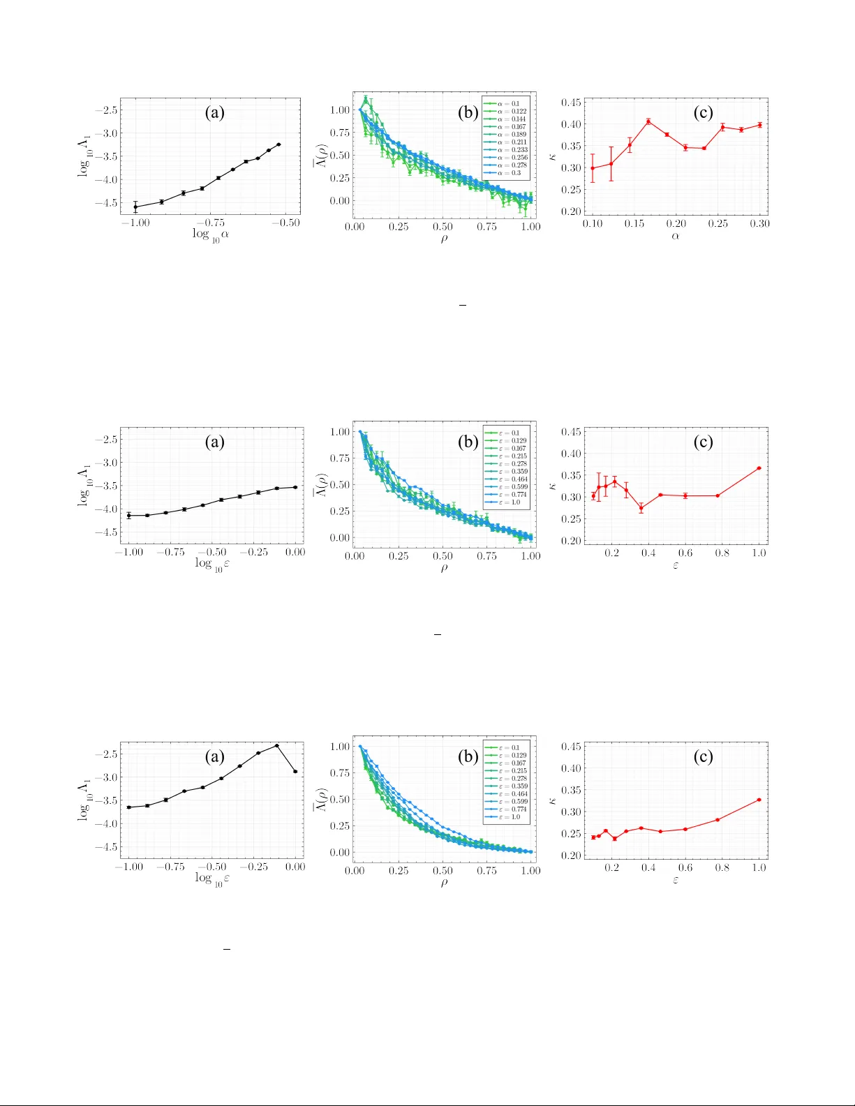
Thermalization of W eakly Nonintegrable FPUT and T oda Dynamics: A L yapunov Spectrum Perspecti ve Aniket Patra 1, 2 and Sergej Flach 1, 3, 4 1 Center for Theor etical Physics of Complex Systems, Institute for Basic Science, Daejeon 34126, Republic of K or ea 2 Department of Physics, Pukyong National University , Busan 48513, Republic of K or ea 3 Basic Science Pr ogram, K or ea University of Science and T echnology (UST), Daejeon, 34113, Republic of Kor ea 4 Centr e for Theor etical Chemistry and Physics, The New Zealand Institute for Advanced Study (NZIAS), Masse y University Albany , Auc kland 0745, New Zealand W e study the thermalization slowing down of Fermi-P ast-Ulam-Tsingou (FPUT) chains and of T oda chains with nonintegrable boundaries. W e focus on the transition from FPUT to harmonic chains, from FPUT to T oda chains with fixed boundaries, and from nonintegrable open boundary T oda to inte grable fixed boundary T oda. W e compute the L yapunov spectrum and analyze its scaling properties upon approaching integrable limits. W e analyze the scaling of the lar gest Laypunov exponent, the rescaled L yapunov spectrum, and the K olmogorov- Sinai entropy . Using additional analytic arguments we demonstrate evidence that all three cases are operating in the regime of a Long Range Network of noninte grable perturbations. I. INTR ODUCTION Conducted more than seventy years ago, the seminal numerical e xperiment of Fermi, Pasta, Ulam, and Tsingou (FPUT) on thermalization in oscillator chains with a quadratic-plus-cubic interaction potential is widely regarded as the first computational in vestigation of nonequilibrium many-body dynamics [ 1 ]. Their simulations sho wed that when the system is initialized in a low- frequency normal mode of the corresponding linear chain, characterized by frequency ω q and wav enumber q , the energy remains confined to a small set of neighboring modes for unexpectedly long times. Equipartition in mode space is e ventually achiev ed, but only on e xceptionally long timescales. Remarkably , despite the dynamics being go verned by a nonlinear Hamiltonian that exhibits chaotic beha vior , the system displays near-recurrences to the initially e xcited mode before thermalizing. These observations stood in sharp contrast to the expectations of statistical mechanics and were initially perceiv ed as para- doxical. The subsequent ef fort to understand this paradox has driven major developments in modern statistical and mathematical physics [ 2 – 6 ]. Indeed, a satisfactory explanation of the FPUT results requires the combined application of powerful theoretical framew orks – including K olmogorov-Arnol’ d-Moser (KAM) theory [ 7 – 18 ], Birkhoff-Gusta vson normal form analysis [ 19 – 23 ], and resonance-overlap criteria [ 24 – 30 ] – together with extensiv e numerical in vestigations enabled by modern computational resources. In the context of the existing FPUT literature, two aspects deserve particular emphasis. First, the ener gy density considered in the original FPUT simulations is quite small, so that the nonlinear, integrability-breaking perturbation can be regarded as weak. Second, the commonly studied initial conditions – where only a small fraction of the low-frequency normal modes of the harmonic chain are excited – are rather atypical. Early works by Izrailev and Chirikov pointed out the existence of a stochasticity thr eshold in energy density [ 24 ]. When this threshold is crossed, nonlinear resonances begin to overlap, gi ving rise to strong dynamical chaos that rapidly drives the system tow ard equipartition and thermal equilibrium [ 25 , 27 – 29 ]. For suf ficiently small energy densities, ho wev er , the application of KAM theory to FPUT -type systems demonstrates the persistence of regular motion and the absence of equipartition below certain thresholds [ 15 – 18 ]. A complementary line of in vestigation, initiated by Zabusk y and Kruskal, relates the recurrence phenomenon observed in the FPUT chain to the emergence of solitons in the K ortewe g-de Vries (KdV) equation and its truncations in mode space [ 31 – 35 ]. Furthermore, the commonly used initial conditions often lie close to the so-called q -breather solutions, which are exact time- periodic stationary solutions of the FPUT chain [ 36 – 39 ]. This proximity to near -integrable regions of phase space (see also [ 40 ]) giv es rise to two distinct dynamical timescales, a phenomenon often referred to as metastability or pr ethermalization [ 41 – 47 ]. On the shorter timescale, the ev olution remains effecti vely noner godic, with energy confined to a small set of modes. Only on a much longer timescale does the system gradually escape this near-inte grable region and recov er the normal statistical beha vior associated with thermal equilibrium. In this paper , we aim to relate the non-KAM dynamics (the rele vance of the non-KAM regime is explained in more detail below) observed in the FPUT chain and related anharmonic lattices to nearby integrable dynamics. T o remain close to the original FPUT setting, we focus on the FPUT - α model, which contains only the cubic nonlinearity . Besides the tri vial inte grable limit provided by the linear chain, another closely related integrable system is the T oda chain [ 48 – 55 ]. Sev eral studies hav e compared the approach to thermal equilibrium in the initially metastable or prethermal regime of the FPUT - α dynamics with the ev olution observed in both the linear and the T oda chains. In particular, the similarity between the metastable FPUT dynamics and the inte grable e v olution of the T oda chain was first pointed out in Ref. [ 56 ]. Subsequent works hav e carried out increasingly detailed comparisons between these models [ 57 – 64 ]. 2 All of these w orks [ 56 – 64 ] lar gely follow the traditional statistical-mechanics approach [ 65 ] of monitoring the time e volution of suitable observables, such as the av erage energy of the normal modes, the normalized spectral entropy , or the total energy . From the beha vior of these quantities one then extracts characteristic time scales, such as the er godization time. It is well kno wn, howe v er , that such analyses can be highly sensitiv e to the choice of observ able and to the specific initial conditions [ 66 ]. In this work, instead, we characterize the weakly nonintegrable dynamics of the FPUT - α chain and related models using univ ersal indicators of chaos: the maximum L yapuno v characteristic exponent (mLCE), the full L yapunov spectrum (LS), and the rescaled Kolmogoro v–Sinai (KS) entropy [ 67 – 73 ]. According to Pesin’ s theorem, the KS entropy can be obtained by summing ov er all positi ve L yapunov exponents [ 74 ]. These quantities are particularly attracti ve because, in addition to being coordinate- independent, they remain in variant under a broad class of transformations [ 67 ]. W e note that Ref. [ 64 ] already employed the mLCE to analyze various FPUT dynamics and to quantify their proximity to either the linear or the T oda chain. In this sense, our work may be viewed as a complementary inv estigation and a natural extension of Ref. [ 64 ]. More importantly , by examining the scaling behavior of the L yapunov spectrum and the rescaled KS entropy as the system approaches a gi ven inte grable limit, we aim to relate these weakly nonintegrable dynamics to the recently identified uni versality classes governing the slo wing down of thermalization [ 75 – 86 ]. These classes are broadly categorized as (i) long-range network (LRN) and (ii) short-range network (SRN). In the LRN case, weak breaking of integrability induces long-range couplings between the conserved actions of the corresponding integrable system, whereas in the SRN case the resulting couplings remain local. It should be noted that the theoretical frame work underlying these univ ersality classes assumes a suf ficiently large phase space dimension and whate ver small but finite energy density so that the KAM theorem no longer constrains the dynamics. In this regime, most in variant tori are destro yed and the motion is expected to occur within a single connected chaotic re gion of phase space. As a result, typical trajectories explore the same accessible region of phase space, leading to dynamical quantities that are largely independent of the specific initial condition [ 87 , 88 ]. In our numerical calculations, the accessible phase-space dimension is limited by the computational cost of computing the full LS. Nev ertheless, we choose an energy density that, while relativ ely small, exceeds the stochasticity threshold corresponding to the system sizes considered, see Ref. [ 58 ]. Operating in this regime, the dynamics is expected to be dominated by a single chaotic component of phase space, so that the LS becomes independent of both the initial condition and the particular fiducial trajectory used in the numerical integration. Finally , we examine ho w boundary conditions af fect the inte grability of the T oda chain. Since integrability is a highly special property , integrable Hamiltonians are typically fine-tuned. F or example, the T oda chain with either periodic or fixed boundary conditions is integrable when the nearest-neighbor interaction potential retains the exponential form originally introduced by T oda. This integrability can be established through the Lax pair construction [ 50 , 51 , 54 , 89 – 92 ]. In particular, the integrability of the fixed-boundary T oda chain can be understood by embedding it into one half of a periodic T oda chain with antisymmetric initial conditions possessing at least three nodes—two at the boundaries and one at the center [ 53 ]. Altering either the boundary conditions or the interaction potential can hav e dramatic consequences for integrability . In particular , the T oda chain with open boundary conditions is not integrable (see also [ 93 ]), e ven though the dif ference between the open and fixed-boundary cases amounts only to tw o interaction terms at the edges. T o elucidate this sensiti vity , we consider a harmonic chain with a single FPUT - α nonlinearity introduced at one lattice site. As argued in the appendix, ev en a single defect can generate a LRN in the space of conserved actions. By interpolating between the open and fix ed-boundary T oda chains and analyzing the scaling properties of the LS and the rescaled KS entropy , we demonstrate that thermalization slo ws down through the LRN mechanism. The paper is org anized as follows. In Sec. II , we introduce the model Hamiltonians, discuss their inte grability properties, and describe how the rele vant integrable limits are approached. In that section, we also define the LS and the rescaled KS entropy , and outline the numerical integration scheme used in our calculations. Section III presents our numerical results, including a comparison of the dynamics of a harmonic chain with a single FPUT - α defect and an analysis of the LRN that emerges when approaching the fixed-boundary T oda chain from the open-boundary case. Finally , we conclude with a discussion of our findings. II. MODELS AND METHODS In Sec. II A , we present the model Hamiltonians studied in this work, highlighting the integrable ones and their ke y properties. Section II B introduces the main indicators of chaos, namely the L yapunov spectrum (LS) and the rescaled K olmogorov–Sinai (KS) entropy . 3 A. Model Hamiltonians and Boundary Conditions W e consider 1D nonlinear lattice chains with the follo wing nearest-neighbor interaction potentials: V lin ( r ) = 1 2 r 2 , (1a) V FPUT - α ( r ) = 1 2 r 2 + α 3 r 3 , (1b) V T oda ( r ) = 1 4 α 2  e 2 αr − 2 αr − 1  , (1c) V exp ( r ) = 1 4 α 2  e 2 αr − 1  . (1d) The first interaction potential ( 1a ) corresponds to the harmonic spring potential obeying Hooke’ s law . The second potential ( 1b ) was introduced by Fermi, Pasta, Ulam, and Tsingou in their celebrated numerical experiment [ 1 ]. The third potential was proposed by T oda [ 48 , 49 ]. The last potential corresponds to the bare exponential T oda interaction before the subtraction of the linear term. Writing the nearest interaction potentials as V int ( r ) , we define the potential of the entire lattice satisfying either the open or fixed-boundary condition as V lattice, FBC = V int ( q 1 ) + " N − 1 X i =1 V int ( q i +1 − q i ) # + V int ( − q N ) , (2a) V lattice, PBC = " N X i =1 V int ( q i +1 − q i ) # with q i + N = q i , (2b) V lattice, OBC = N − 1 X i =1 V int ( q i +1 − q i ) , (2c) where q i denotes the displacement of the i th mass from equilibrium. This implies that V lattice, FBC = V lattice, OBC + [ V int ( q 1 ) + V int ( − q N )] . (3) W e write 1D lattice Hamiltonians using the lattice potential ( 2 ) introduced abov e as H lattice ( q , p ) = " N X i =1 p 2 i 2 # + V lattice ( q ) ≡ T lattice ( p ) + V lattice ( q ) , (4) where the canonical coordinates and momenta for the N de grees of freedom are denoted by q = { q 1 , . . . , q N } and p = { p 1 , . . . , p N } , with p i representing the momentum conjugate to the lattice displacement q i . Here T lattice ( p ) denotes the kinetic energy of the lattice. The integrability of the harmonic chain with interaction potential ( 1a ), under fixed, periodic, or open-boundary conditions, is most directly established by constructing the action–angle variables, which are obtained through the normal mode decomposition (see Appendix A ). The FPUT - α chain, in contrast, is not integrable. When T oda first introduced his eponymous lattice, he obtained a number of exact soliton solutions [ 48 , 49 ]. The complete integrability of the periodic T oda lattice was later established through the construction of a Lax representation [ 50 , 51 , 94 ]. T o deriv e this representation, one begins with the 2 N Hamilton equations of motion ˙ q = ∂ H ∂ p , ˙ p = − ∂ H ∂ q , (5) which can be compactly written as ˙ z = L H z = { H , z } , (6) where z = ( q , p ) , and the Liouvillian operator L H is defined through the Poisson bracket { A, B } = ∂ A ∂ q ∂ B ∂ p − ∂ B ∂ q ∂ A ∂ p . (7) 4 Introducing the Flaschka variables [ 50 ] a j = 1 2 e α ( q j +1 − q j ) , b j = αp j , (8) the equations of motion deriv ed from Eq. ( 5 ) take the form ˙ a j = a j ( b j +1 − b j ) , ˙ b j = 2  a 2 j − a 2 j − 1  . (9) These equations can be recast as the Lax equation [ 50 , 51 , 94 ] ˙ L = [ B , L ] ≡ B L − LB , (10) where L ( a , b ) is a symmetric N × N matrix and B ( a , b ) is a sk ew-symmetric matrix function of the same dimension. It follows that L ( t ) remains similar to L (0) , implying that the eigenv alues of L are conserved in time. It is therefore conv enient to introduce the conserved quantities I k = 1 k ! T race  L k  , 1 ≤ k ≤ N . (11) which form a complete set of integrals of motion. One readily verifies that I 1 corresponds to the total momentum, while I 2 equals the total ener gy up to an additi ve constant for the periodic T oda chain. The higher integrals become increasingly complicated and correspond to nonlocal quantities in the original lattice variables. In fact, a set of action-angle v ariables was constructed in Ref. [ 52 ] using the discriminant of the Lax matrix L , denoted by ∆( λ ) , defined through det ( λ 1 − L ) =   N Y j =1 a j   [∆( λ ) − 2] . (12) The k th action variable can then be written (see also [ 56 ]) as J k = 2 π ˆ Λ 2 k Λ 2 k +1 cosh − 1  | ∆( λ ) | 2  dλ, (13) where Λ k are the consecutiv ely ordered roots of ∆( λ ) = ± 2 . These action variables are manifestly nonlocal when expressed in terms of the original lattice variables. Follo wing Ref. [ 53 ], the inte grals of motion for the fixed-boundary T oda chain with N lattice sites can be obtained by embed- ding it into a periodic lattice with (2 N + 2) sites labeled by j = − N , . . . , N + 1 . On this extended periodic lattice we impose the antisymmetric initial conditions q − j = − q j , p − j = − p j , q 0 = q N +1 = 0 , p 0 = p N +1 = 0 , (14) for j = 1 , . . . , N , where q j and p j are otherwise arbitrary for these indices. Because the equations of motion preserve this antisymmetry , the segment of the periodic lattice between j = 1 and j = N e volves e xactly as a fixed-boundary T oda chain with N sites. The periodic system possesses 2( N + 1) integrals of motion, which we denote by I ′ k for k = 1 , 2 , . . . , 2( N + 1) , where the prime indicates that the antisymmetric constraint ( 14 ) has been imposed. Under this constraint all integrals with odd k v anish identically , while one additional inte gral reduces to a constant independent of the dynamical variables. Consequently , the fixed-boundary T oda chain is integrable and is characterized by the N nontrivial integrals I ′ k with k = 2 , 4 , . . . , 2 N . Having discussed the integrability of the periodic and fixed-boundary T oda chains, we no w turn to the open-boundary case. Before proceeding, we note the following relations between the T oda and bare exponential interaction potentials: V T oda, PBC = V exp, PBC , (15a) V T oda, FBC = V exp, FBC , (15b) V T oda, OBC = V exp, OBC + 1 2 α ( q 1 − q N ) . (15c) It is well kno wn that the bare e xponential T oda lattice is integrable under all three boundary conditions. For open boundaries the Lax matrices L and B are tridiagonal [ 54 ]. In the periodic case they remain tridiagonal in the bulk but acquire additional corner elements L 1 N = L N 1 = − B 1 N = B N 1 = a N [ 50 ]. The same Lax construction fails for H T oda, OBC because of the additional linear term in Eq. ( 15c ); see [ 93 ] for a simple proof. Consequently , the open-boundary T oda lattice is not inte grable, a conclusion also supported by the presence of a positive maximum L yapunov characteristic exponent. Notably , unlik e the FPUT - α model – where where all intersite interactions differ from those of the integrable T oda chain (e.g., the fix ed-boundary one) – the open-boundary T oda lattice departs from the integrable case only through tw o boundary interaction terms, see Eq. ( 3 ). 5 B. L yapunov Spectrum and K olmogor ov–Sinai Entropy W e quantify the nonintegrability – manifested as the sensiti ve dependence of trajectories on initial conditions – by computing the L yapunov spectrum (LS) and related chaotic indicators for the Hamiltonians considered here. As noted in the introduction, these quantities possess univ ersal properties: their asymptotic values are in v ariant under smooth canonical transformations and are largely independent of the choice of initial conditions [ 67 ]. In this section, we briefly revie w the rele v ant theoretical results and describe the procedure used to compute them [ 71 , 73 ]. T o compute the L yapunov characteristic exponents (LCEs), we first derive the ev olution equation for infinitesimal perturba- tions by linearizing Hamilton’ s equations ( 6 ). This yields the v ariational equation ˙ w ( t ) =  Ω 2 N · D 2 H ( z ( t ))  · w ( t ) , (16) where w ( t ) = ( δ q ( t ) , δ p ( t )) = ( δ q 1 ( t ) , . . . , δ q N ( t ) , δ p 1 ( t ) , . . . , δ p N ( t )) is an infinitesimal de viation from the trajectory z ( t ) = ( q ( t ) , p ( t )) . The matrix D 2 H ( z ( t )) denotes the Hessian of the Hamiltonian e v aluated along the trajectory ,  D 2 H ( z ( t ))  i,j = ∂ 2 H ∂ z i ∂ z j     z ( t ) , i, j = 1 , . . . , 2 N , (17) while the symplectic identity matrix is Ω 2 N =  O N 1 N − 1 N O N  , (18) where 1 N and O N denote N × N identity and null matrices, and Ω 2 2 N = − 1 2 N . From Eq. ( 16 ), the generator of the tangent dynamics is A ( z , t ) ≡ Ω 2 N · D H 2 ( z ( t )) . (19) Since the Hessian is symmetric, D 2 H ( z ( t )) =  D 2 H ( z ( t ))  T , it follows that A T ( z , t ) · Ω 2 N + Ω 2 N · A ( z , t ) = 0 , (20) where we used Ω 2 2 N = − 1 2 N . Hence A ( z , t ) belongs to the symplectic Lie algebra sp (2 N , R ) . For a short time step δ t , the infinitesimal Jacobian J ( z , t ) ≈ exp [ A ( z , t ) δ t ] , (21) is therefore symplectic, i.e., J ( z , t ) ∈ S p (2 N , R ) , and satisfies J ( z , t ) · Ω 2 N · J T ( z , t ) = Ω 2 N . (22) The variational equations ( 16 ) form a system of linear differential equations for w . Their main complication lies in the time dependence of the coefficients through the instantaneous generator A ( z , t ) . The solution at t = T end can nevertheless be obtained by integrating the equations, yielding w ( T end ) = J ( z 0 , T end ) · w (0) , (23) where z (0) ≡ z 0 is the initial phase-space point and the Jacobian matrix J ( z 0 , T end ) is expressed through the time-ordered exponential T exp as in J ( z 0 , T end ) = T exp " ˆ T end 0 dt J ( z ( t ) , t ) # . (24) For the numerical computation of the LCEs, the full Jacobian is approximated as in J ( z 0 , T end ) = lim N step →∞ N step − 1 Y k =0 J ( z ( k δ t ) , k δ t ) = lim N step →∞ N step − 1 Y k =0 exp [ A ( z ( k δ t ) , k δ t ) δ t ] , (25) with T end = N step δ t and δ t → 0 the integration time step. Using Eq. ( 25 ) together with the fact that the product of symplectic matrices is symplectic, it follows that the full Jacobian J ( z 0 , T end ) of the tangent flow is also symplectic. 6 Since the LCEs characterize the asymptotic average rate of growth (or decay) of infinitesimal perturbations, we consider the norm squared of the perturbation vectors w ( t ) . From ∥ w ( t ) ∥ = w T (0) · J T ( z 0 , T end ) · J ( z 0 , T end ) · w (0) , (26) the ev olution of w ( t ) is gov erned by the real, symmetric, positi ve-definite matrix defined in M ( z 0 , T end ) = J T ( z 0 , T end ) · J ( z 0 , T end ) . (27) The Oseledets Multiplicative Ergodic Theorem (MET) [ 68 ] then states that, for a statistically stationary and ergodic sequence of matrices generated by the underlying ergodic flo w z ( t ) , the limit in lim T end →∞ [ M ( z 0 , T end )] 1 / 2 T end = P (28) exists. In the non-KAM dynamical regime of interest, where the chaotic re gion of phase space is fully connected, the matrix P becomes independent of the initial phase-space point. It has 2 N positiv e eigen v alues µ 1 ⩾ µ 2 ⩾ . . . ⩾ µ 2 N , from which the L yapunov spectrum is obtained via Λ k = ln µ k . (29) for k = 1 , . . . , 2 N . Because the Jacobian is symplectic, if µ is an eigenv alue of M , then so is 1 /µ . Consequently , each positiv e L yapunov exponent Λ i is paired with a neg ativ e one, Λ 2 N − i +1 = − Λ i , reflecting the preservation of phase-space volume. It is therefore sufficient to analyze the rescaled positiv e LCEs Λ i ≡ Λ i / Λ 1 to identify the universality classes associated with thermalization slowdo wn [ 81 , 83 ]. Accordingly , we plot the normalized spectrum Λ( ρ ) versus ρ = i/ N in Figs. 1 , 2 , and 3 . Moreover , the ke y features relev ant for understanding thermalization slo wdown are succinctly captured by the beha vior of the rescaled K olmogorov-Sinai (KS) entropy , κ = 1 N N X i =1 Λ i − − − − → N →∞ ˆ 1 0 Λ( ρ ) dρ, (30) obtained from the LS. W e conclude this section by summarizing the e xpected behavior of the LCEs in the two uni versality classes of thermalization slowdo wn [ 83 ]. In the long-range network (LRN) class, the maximal exponent Λ 1 vanishes – typically as a power law – while the rescaled spectrum Λ( ρ ) con ver ges to a limiting curve that itself decays as a power law in ρ as the inte grable limit is approached. Consequently , the rescaled KS entropy κ approaches a finite constant. In contrast, in the short-range network (SRN) class, although Λ 1 again vanishes algebraically , the rescaled spectra do not con ver ge. Instead, they are well described by an exponential form Λ( ρ ) ∼ e − β ρ , with β di ver ging as the integrability-breaking parameter tends to zero. Correspondingly , κ → 0 as 1 /β in the integrable limit. C. Computational Framework: Split-Step Integration and L yapunov Analysis In our numerical algorithm for computing the LS [ 69 – 73 ], we first consider the finite-time maximal L yapunov characteristic exponent of order p , denoted by Λ p ( t ) . This quantity measures the exponential rate at which the volume of a p -dimensional parallelogram, spanned by p linearly independent deviation vectors w 1 ( t ) , w 2 ( t ) , . . . , w p ( t ) , ev olves in time. It is defined as in Λ p ( T end ) = 1 T end N step X j =1 ln  vol p [ w 1 ( j δ t ) , w 2 ( j δ t ) , . . . , w p ( j δ t )] vol p [ w 1 (( j − 1) δ t ) , w 2 (( j − 1) δ t ) , . . . , w p (( j − 1) δ t )]  , (31) where vol p [ · ] denotes the volume of the p -parallelogram formed by the gi ven vectors. T aking the infinite-time limit, Λ p 1 = lim T end →∞ Λ p ( T end ) , (32) yields the maximal L yapunov characteristic exponent of order p ( p -mLCE). Starting from an orthonormal set of deviation vectors { w 1 (0) , w 2 (0) , . . . , w p (0) } , their time ev olution over a step δ t produces the set { w 1 ( δ t ) , w 2 ( δ t ) , . . . , w p ( δ t ) } , which is generally no longer orthonormal. The vectors must therefore be reorthonormal- ized before further ev olution. This can be achiev ed through Gram–Schmidt orthonormalization and applied iterativ ely while 7 FIG. 1. Fixed boundary condition FPUT - α with N = 32 . W e perform the calculations starting from an initial condition with all lattice displacements set to zero, while the lattice momenta are randomly drawn subject to the constraint that the energy density equals 0.1. As the integrable limit H lin,FBC is approached by decreasing α , the maximum L yapunov characteristic exponent (mLCE) Λ 1 steadily decreases, as shown in panel (a). In panel (b), we plot the rescaled L yapunov spectra (LS) Λ( ρ ) ≡ Λ i / Λ 1 as a function of ρ = i/ N , with i = 1 , . . . , N , for values of α equally spaced between 0.1 and 0.3. The area under these spectra appears to saturate to a finite value, consistent with the beha vior of the rescaled Kolmogoro v–Sinai entropy κ sho wn in panel (c). This scaling of the L yapuno v spectra indicates that thermalization slows down according to the long-range network (LRN) scenario. FIG. 2. W e interpolate between the nonintegrable FPUT - α chain and the integrable T oda chain by tuning the parameter ε , imposing fix ed boundary conditions in both cases. The potential is gi ven by Eq. ( 43 ) with N = 32 , and the initial condition is the same as in Fig. 1 . The parameter ε is sampled at logarithmically spaced v alues between 0.1 and 1.0. As in Fig. 1 , panels (a), (b), and (c) show the maximal L yapuno v characteristic exponent (mLCE) Λ 1 , the rescaled L yapuno v spectrum Λ( ρ ) ≡ Λ i / Λ 1 as a function of ρ = i/ N ( i = 1 , . . . , N ) , and the rescaled K olmogorov–Sinai (KS) entropy κ , respectively . As before, the results indicate that thermalization slows do wn in accordance with the long-range network (LRN) scenario. FIG. 3. Mixed boundary condition T oda chain with N = 32 . The potential is taken as in Eq. ( 44 ), whose integrable limit corresponds to the fixed-boundary T oda chain. The initial condition is identical to that used in Fig. 1 . The parameter ε is varied ov er logarithmically spaced v alues in the interval 0 . 1 ⩽ ε ⩽ 1 . 0 . Panels (a), (b), and (c) display the maximal L yapunov characteristic exponent (mLCE) Λ 1 , the rescaled L yapunov spectrum Λ( ρ ) ≡ Λ i / Λ 1 as a function of ρ = i/ N ( i = 1 , . . . , N ) , and the rescaled Kolmogoro v–Sinai (KS) entropy κ , respectiv ely . The results again support the picture that thermalization becomes progressi vely slo wer , consistent with the long-range network (LRN) mechanism. 8 following a fiduciary trajectory z ( t ) . Besides pre venting numerical overflo w , this renormalization aligns the deviation v ectors with the most unstable directions, allowing the p -mLCEs to con verge more rapidly . In practice, ho wev er , the Gram–Schmidt procedure may suffer from numerical instabilities. Therefore, following Refs. [ 71 – 73 , 83 ], we instead perform a QR decomposition of the 2 N × p matrices defined in W ( j δ t ) =  w 1 ( j δ t ) w 2 ( j δ t ) · · · w p ( j δ t )  , (33) at each step j = 1 , 2 , . . . , N step . This provides a numerically stable way to obtain the expansion coef ficients of the evolving p -parallelograms along the fiducial trajectory , without explicitly computing their spanning vectors. The individual LCEs, which together form the full LS, are then obtained from Λ p = Λ p 1 − Λ p − 1 1 , (34) with Λ 0 1 ≡ Λ 1 the maximal LCE computed using Λ 1 = lim N step →∞ 1 N step δ t k X j =1 ln ∥ w ( j δ t ) ∥ ∥ w (( j − 1) δ t ) ∥ . (35) Here ∥ w ( j δ t ) ∥ denotes the magnitude of the deviation vector at time t = j δ t , where δ t is the step size used in e valuating all Λ p 1 . W e employ split-step symplectic inte gration schemes to compute the fiducial trajectory from Hamilton’ s equations. In these methods, the Hamiltonian is decomposed into exactly solvable parts, and the time ev olution is constructed through successiv e applications of their individual propag ators [ 95 – 107 ]. Formally , the solution of Eq. ( 6 ) can be written as in z ( t ) = e tL H z (0) = + ∞ X s =0 t s s ! ( L H ) s z (0) . (36) In split-step schemes, the operator e tL H is approximated so that phase-space volume is preserved at each time step; con- sequently , ev ery step of the map corresponds to a canonical transformation. The lattice Hamiltonians considered here can be written as H = A + B , where A is the total kinetic energy and B is the total potential energy . For this decomposition, the operators e tL A and e tL B are known e xplicitly in closed form. Using the Baker–Campbell–Hausdorf f formula, the operator e δ tL H is approximated as in e δ tL H = k Y j =1 e a j L A δ t e b j L B δ t + O ( τ p ) , (37) where the coefficients a 1 , b 1 , a 2 , b 2 , ..., a k , b k satisfy the consistency conditions P k j =1 a j = P k j =1 b j = 1 . The accuracy of the approximation is determined by the order p , which depends on k and and on the choice of these coefficients. W e compute the LS using the tangent map method of Ref. [ 70 ], in which the same split-step integrator is applied to both the phase-space trajectory and the variational flo w . The flow equations corresponding to the A and B steps are given in ˙ q = p , ˙ p = 0 , ˙ δ q = δ p , ˙ δ p = 0 ,            ⇒ d z dt = L A z , ˙ q = 0 , ˙ p = − ∂ V ( q ) ∂ q , ˙ δ q = 0 , ˙ δ p = − D 2 V ( q ) δ q ,                ⇒ d z dt = L B z , (38) where the Hessian of the potential, D 2 V ( q ( t )) j k = ∂ 2 V ( q ) ∂ q j ∂ q k     q ( t ) , j, k = 1 , 2 , . . . , N , (39) appears. The A step reduces to a system of simple ordinary differential equations (ODEs) with constant coefficients and can therefore be solved straightforwardly . During the B step, o ver the interval [ t 0 , t 0 + b j δ t ] , the coordinates q remain constant. Consequently , the gradient and Hessian of the potential, ∂ V ( q ) ∂ q = ∂ V ( q ) ∂ q     q ( t )= q ( t 0 ) , D 2 V ( q ( t )) = ∂ 2 V ( q ) ∂ q j ∂ q k     q ( t )= q ( t 0 ) , j, k = 1 , . . . , N , (40) 9 FIG. 4. W e plot log 10 Λ 1 , where Λ 1 denotes the maximal L yapuno v characteristic exponent (mLCE), as a function of in verse system size 1 / N for three models: the fixed-boundary FPUT - α chain (blue circles), a linear chain with a single FPUT - α nonlinearity on the bond between sites N / 2 and N/ 2 + 1 (teal hexagons), and the open-boundary T oda chain (red stars). In all three cases, the nonlinearity parameter is fixed to α = 0 . 25 . The initial conditions are randomly chosen at fixed energy density E / N = 0 . 1 , following the procedure used in Figs. 1 , 2 , and 3 . For the FPUT - α chain, Λ 1 shows almost no dependence on N . In contrast, for the other two models Λ 1 approaches a finite saturation v alue with increasing N , i.e., log 10 Λ 1 tends to a constant as 1 / N → 0 . remain constant, so the corresponding flow equations reduce to ODEs with constant coefficients. This considerably simplifies the implementation, since in both steps one only needs to solve linear systems of ODEs with constant coef ficients. The fourth-order symplectic integration scheme used in this work is the AB A 864 method, first introduced in Ref. [ 104 ]. Follo wing Ref. [ 104 ], we express e δ tL H as in e δ tL H = e a 1 L A δ t e b 1 L B δ t e a 2 L A δ t e b 2 L B δ t e a 3 L A δ t e b 3 L B δ t × e a 4 L A δ t e b 4 L B δ t e a 4 L A δ t × e b 3 L B δ t e a 3 L A δ t e b 2 L B δ t e a 2 L A δ t e b 1 L B δ t e a 1 L A δ t + O  δ t 4  (41) for a time step δ t . Note the palindromic sequence formed by the splitting coefficients, ensuring symmetry and exact time rev ersibility . T runcating the values reported in T able 3 of Ref. [ 104 ] to eight decimal places, the coef ficients in Eq. ( 41 ), { a 1 , a 2 , a 3 , a 4 , b 1 , b 2 , b 3 , b 4 } , are giv en in (see also [ 106 , 107 ]) a 1 = 0 . 07113343 , b 1 = 0 . 18308368 , a 2 = 0 . 24115343 , b 2 = 0 . 31078286 , a 3 = 0 . 52141176 , b 3 = − 0 . 02656462 , a 4 = − 0 . 33369862 . b 4 = 0 . 06539614 . (42) III. CHA O TIC PR OPER TIES OF THE INTERPOLA TING LA TTICE MODELS In this section, we calculate the L yapunov spectrum (LS) for the following three scenarios: 1. W e first consider the FPUT - α potential with fixed boundary conditions, V FPUT - α, FBC , in the limit α → 0 , where the system approaches the inte grable linear chain since V FPUT - α, FBC ( α = 0) = V lin , FBC . In Fig. 1 we compute the LS for ten linearly spaced values of α in the range 0 . 1 ≤ α ≤ 0 . 3 . Because the FPUT - α potential is unbounded from belo w , the parameter range must be restricted; for α ≳ 0 . 3 the chain becomes unstable and undergoes breakdo wn [ 108 ]. 2. An interpolation between the fix ed-boundary T oda and FPUT - α chains using the mixed potential defined in V Mixed, FBC = (1 − ε ) V T ,FBC + εV FPUT - α , FBC , (43) with 0 < ε < 1 . Here ε = 0 corresponds to the inte grable fixed-boundary T oda chain, while ε = 1 yields the nonintegrable fixed-boundary FPUT - α chain. Figure 2 sho ws the LS computed for ten values of ε between 0 . 1 and 1 . 0 , chosen to be equally spaced on a logarithmic scale. 10 FIG. 5. Rescaled L yapunov spectra Λ( ρ ) ≡ Λ i / Λ 1 as a function of ρ = i/ N ( i = 1 , . . . , N ) for open-boundary T oda chains at increasing system sizes. Results are obtained from random initial conditions at fixed energy density E / N = 0 . 1 for N = 32 , 40 , 48 , 56 , 64 , and 128 . The spectra exhibit negligible dependence on N . The inset shows the rescaled K olmogorov-Sinai (KS) entropy κ as a function of 1 / N , highlighting the con ver gence of the Λ( ρ ) curves with increasing system size (cf. the (c) panels of Figs. 1 , 2 , and 3 ). 3. The mix ed-boundary T oda potential V T ,Mix ed (see Fig. 3 ) defined in V T oda, Mixed = V T oda, FBC − ε [ V T oda ( q 1 ) + V T oda ( − q N )] , (44) considered in the limit ε → 0 . The case ε = 0 corresponds to the integrable fixed-boundary T oda chain, while ε = 1 yields the nonintegrable open-boundary T oda chain. In Fig. 3 we compute the LS for the same values of ε used in Fig. 2 . All L yapunov characteristic e xponent (LCE) calculations are performed using the AB A 864 algorithm with parameters δ t = 0 . 32 , T end = 10 6 , and energy density E / N = 0 . 1 . The timestep and integration time are chosen such that the LS reaches clear saturation. In addition, the minimum v alues of α and ε are selected to ensure that the LS con verges within the integration window t ≤ T end . T o quantify conv ergence, we estimate the uncertainties δ Λ i from the standard deviation of the time-dependent exponents Λ i ( t ) over the window t ∈ [ T end / 10 , T end ] . Standard error-propag ation is then used to obtain the uncertainties in log 10 Λ 1 , Λ( ρ ) , and κ . It is well known that numerical simulations of integrable Hamiltonian systems with split-step symplectic integrators gener - ically break inte grability and can induce timestep- and integrator-dependent Trotter chaos [ 86 , 107 ]. Since integrable systems hav e v anishing LCEs, even a small spurious saturation value can be significant. In strongly chaotic systems such effects are typically negligible compared with the intrinsic LCEs. Howe ver , near inte grability such protection is not guaranteed. W e ne ver - theless find that our choice of δ t , T end , and the fourth-order symplectic scheme AB A 864 suppresses T rotter-induced artifacts to a negligible le vel [ 107 ]. W e no w specify the initial conditions. Throughout, we use random initial conditions at fixed ener gy density E / N ≡ h = 0 . 1 . All lattice displacements are set to zero, q j = 0 . The momenta are generated by first sampling N random numbers p 0 j uniformly from [0 , 1) and removing the mean, p j = p 0 j − p 0 , where p 0 =  P N j =1 p 0 j  / N . The physical momenta are then obtained by rescaling p j =  hN H lattice ( q = 0 , p = p )  1 / 2 p j , with h = 0 . 1 . This construction yields random initial conditions with the desired energy density irrespecti ve of the form of H lattice . W e fix the random-number generator and seed to produce a single realization, which is used in all three scenarios sho wn in Figs. 1 , 2 , and 3 . As emphasized in the Introduction, our goal is to probe the universality classes of weakly nonintegrable thermalization slo w- down beyond the KAM regime. For the FPUT - α chain and related systems, this requires choosing an ener gy density E / N abov e the stochasticity threshold h c [ 24 , 25 , 27 – 29 ]. For random initial conditions, Ref. [ 58 ] estimates h c ∝ N − 2 . The FPUT - α chain can also be viewed as a perturbation of the linear chain with effecti ve strength | α | √ h [ 30 , 64 ], suggesting that the stochasticity crossov er occurs when | α | √ h reaches a size-dependent threshold. Combining these considerations yields h c ∼ C / ( α 2 N 2 ) . T aking C = O (1) giv es h c ≈ 1 . 6 × 10 − 2 for the parameters used here. Consistently , the analysis of Λ 1 in Ref. [ 58 ] places the threshold in the range 10 − 3 < h c < 10 − 2 (see Fig. 6 of [ 58 ]). These estimates indicate that our choice E / N = 0 . 1 lies safely abov e the stochasticity threshold while remaining in the weakly nonintegrable regime. 11 T o determine the network class of the three cases introduced above, we compute the positiv e part of the rescaled L yapunov spectrum Λ( ρ ) ≡ Λ i / Λ 1 with ρ = i/ N and i = 1 , . . . , N , as defined below Eq. ( 29 ). The rescaled Kolmogoro v–Sinai (KS) entropy κ is then obtained from Eq. ( 30 ). Figures 1 , 2 , and 3 show: (a) log – log plots of Λ 1 versus the control parameters α or ε gov erning the approach to integrability , (b) the curves Λ( ρ ) v ersus ρ , and (c) the rescaled KS entropy κ versus the same control parameter . The three figures exhibit remarkably similar behavior . Panel (a) shows that Λ 1 decreases monotonically as the integrable limit is approached. In panel (b), the curves Λ( ρ ) progressiv ely collapse onto a common profile as α or ε is reduced toward integrability . The limiting curves display a power-la w decay of Λ( ρ ) with ρ , consistent with the behavior reported in Ref. [ 83 ]. This conv ergence is further supported by panel (c), where the rescaled KS entropy κ approaches a finite constant as the system approaches integrability . Since κ is simply the area under the Λ( ρ ) – ρ curve [Eq. ( 30 )], the saturation of κ corroborates the collapse of the spectra. T ogether, these indicators point to a slo wdown in thermalization through the long-range network (LRN) pathway in all three scenarios. Recall from the Introduction that the LRN scenario arises when breaking integrability couples an extensi v e number of actions. In the first two cases – approaching the fixed-boundary harmonic and T oda limits from the fixed-boundary FPUT - α chain – the emergence of the LRN class is therefore natural. The actions of both the T oda and harmonic chains are highly nonlocal in lattice space, as sho wn in Eqs. ( 13 ) and ( A4 ). Consequently , e ven weak departures from these inte grable limits couple man y actions simultaneously , leading to the observed LRN thermalization slo wdown. More surprising is the appearance of the LRN class when approaching the fixed-boundary T oda chain from the open-boundary one. As seen from Eq. ( 44 ), the open-boundary T oda potential differs from the fixed-boundary case only by two boundary terms. One might therefore expect that breaking integrability through such a small number of local perturbations would produce chaos that v anishes in the thermodynamic limit. Ho wev er , Fig. 4 sho ws that Λ 1 instead saturates to a finite value as the system size N increases for both models where integrability is broken locally . In addition, we compute the rescaled L yapunov spectra for open-boundary T oda chains at increasing system sizes in Fig. 5 , starting from random initial conditions with fixed energy density E / N = 0 . 1 . These spectra exhibit only weak dependence on N . This behavior can be understood by comparing the linear chain with a single FPUT - α nonlinearity to the full FPUT - α chain, as discussed in Appendix A . By counting the number of terms in the perturbation, one finds that the ef fecti ve perturbation strength of a single FPUT - α defect is comparable to that of the fully nonlinear chain, owing to the nonlocal structure of the linear-chain actions. The same reasoning applies to the open-boundary T oda chain, explaining the emergence of the LRN class in that case as well. IV . SUMMAR Y AND OUTLOOK W e conclude by summarizing our main results. W e have in vestig ated thermalization slowdo wn in three scenarios. In the first two, the inte grable fixed-boundary harmonic and T oda chains are approached from the fix ed-boundary FPUT - α chain, while in the third the fixed-boundary T oda chain is approached from the open-boundary T oda chain. In all cases, the scaling properties of the L yapunov spectra (LS) demonstrate that the slowdo wn occurs through the long-range network (LRN) pathw ay . One important scenario not addressed here is the approach to integrability in the fixed-boundary FPUT - α chain by decreasing the energy density . This problem is more subtle because the system admits two integrable limits – the linear chain and the T oda chain – and because the dynamics may enter a KAM regime. Understanding how the KAM regime affects the two network classes of thermalization slowdo wn would therefore be an important direction for future w ork. Another open question concerns the role of the nonuniqueness of action–angle representations in determining the scaling properties of the LS. For example, Ref. [ 54 ] shows that the open-boundary T oda lattice with bare exponential interactions is superintegrable: a chain with N sites possesses (2 N − 1) independent integrals of motion. As a consequence, the actions obtained from the Hamilton–Jacobi equations are not unique in this model. It would be interesting to determine how the LS behav es when this integrable limit is approached from a noninte grable system such as the open-boundary T oda chain. A related direction is to explore networks associated with integrable chains that host flat bands [ 109 – 111 ]. A flat-band normal- mode spectrum implies strong degeneracies in action space. In contrast to the partial degeneracy of the open-boundary T oda lattice, the degenerac y here appears to be maximal. Whether such systems gi ve rise to a distinct network class of thermalization slowdo wn remains an intriguing open question. Appendix A: FPUT - α Lattice in T erms of Harmonic Chain Actions and Angles Consider the classical harmonic chain Hamiltonian with fixed boundary condition H lin, FBC = N X j =0 " p 2 j 2 + 1 2 ( q j +1 − q j ) 2 # , (A1) 12 where we hav e q 0 = q N +1 = p 0 = p N +1 = 0 . W e introduce the normal mode positions and momenta for this Hamiltonian as  q j p j  = r 2 N + 1 N X k =1  Q k P k  sin  π k j N + 1  : = r 2 N + 1 N X k =1  Q k P k  sin (2 α k j ) , (A2) where the variable α k = π k 2( N + 1) (A3) is introduced for later con venience. The normal mode variables ( A2 ) can then be related to the actions and angles of the harmonic chain as Q k = p 2 J k sin θ k , P k = ω k p 2 J k cos θ k , (A4) where ω k = 2 sin  π k 2( N + 1)  : = 2 sin ( α k ) . (A5) Equation ( A1 ) can then be rewritten in terms of these ne w v ariables as H lin, FBC = N X k =1 P 2 k + ω 2 k Q 2 k 2 = N X k =1 ω 2 k J k . (A6) W e want to treat H FPUT - α , FBC as a perturbation over H lin, FBC . T o do so, we recast H FPUT - α , FBC in terms of J k and θ k from Eq. ( A4 ). W e start by rewriting the nonlinear term in the potential as ∆ V FPUT - α , FBC = N X j =0 α 3 ( q j +1 − q j ) 3 ≡ N X j =0 α 3 (∆ q j ) 3 . (A7) W e write ∆ q i in terms of the coordinates of the normal mode as ∆ q j = r 2 N + 1 N X k =1 Q k [sin (2 α k ( j + 1)) − sin (2 α k j )] = N X k =1 c k cos [(2 j + 1) α k ] , (A8) where c k = 2 r 2 N + 1 Q k sin α k . (A9) In the final line of Eq. ( A8 ) we hav e used sin A − sin B = 2 cos  A + B 2  sin  A − B 2  . (A10) Cubing both sides of Eq. ( A8 ), we obtain (∆ q j ) 3 = X k 1 ,k 2 ,k 3 c k 1 c k 2 c k 3 3 Y r =1 cos [(2 j + 1) α k r ] = 1 4 X k 1 ,k 2 ,k 3 c k 1 c k 2 c k 3 X σ 1 ,σ 2 ∈{± 1 } cos [(2 j + 1)Λ( k , σ )] = 1 √ 2 1 ( N + 1) 3 / 2 X k 1 ,k 2 ,k 3 Q k 1 Q k 2 Q k 3 ω k 1 ω k 2 ω k 3 X σ 1 ,σ 2 ∈{± 1 } cos [(2 j + 1)Λ( k , σ )] (A11) where Λ( k , σ ) : = α k 1 + σ 1 α k 2 + σ 2 α k 3 . (A12) 13 In the last line of Eq. ( A11 ), we hav e used cos A cos B cos C = 1 4 [cos ( A + B + C ) + cos ( A + B − C ) + cos ( A − B + C ) + cos ( A − B − C )] . (A13) In order to obtain an expression for ∆ V FPUT - α , FBC , we need to ev aluate P N j =0 (∆ q j ) 3 . T o that end, we note that S ( N , k , σ ) = N X j =0 cos [(2 j + 1)Λ( k , σ )] = Re   N X j =0 e i (2 j +1)Λ( k , σ )   = Re  e i Λ( k , σ ) 1 − e 2 i ( N +1)Λ( k , σ ) 1 − e 2 i Λ( k , σ )  = sin [2( N + 1)Λ( k , σ )] 2 sin [Λ( k , σ )] = sin [ π ( k 1 + σ 1 k 2 + σ 2 k 3 ) | {z } integer:= k ( k , σ ) ] / 2 sin [Λ( k , σ )] . (A14) As a result, the above sum v anishes unless Λ( k , σ ) = nπ , where n is an integer . Because the cos function is ev en and π - antiperiodic, restricting Λ( k , σ ) into the domain [0 , π ] is enough to obtain all the possible values of S ( N , k , σ ) . Using this, we hav e S ( N , k , σ ) =      N + 1 , if Λ( k , σ ) = 0 , − ( N + 1) , if Λ( k , σ ) = π , 0 , otherwise. (A15) In terms of k and σ , we translate the resonance conditions of ( A15 ) as follows: Λ( k , σ ) = 0 ⇐ ⇒ k ( k , σ ) = 0 ⇐ ⇒ k 3 = k 1 + k 2 , k 2 = k 3 + k 1 , k 1 = k 2 + k 3 , (A16a) Λ( k , σ ) = π ⇐ ⇒ k ( k , σ ) = 2( N + 1) ⇐ ⇒ k 1 + k 2 + k 3 = 2( N + 1) . (A16b) Equation ( A16 ) lists all the different choices of σ for a giv en k , for which S ( N , k , σ )  = 0 . Putting Eqs. ( A7 ), ( A11 ), ( A15 ), and ( A16 ) together , we obtain ∆ V FPUT - α , FBC = α 12 X k , σ c k 1 c k 2 c k 3 N X j =0 cos [(2 j + 1)Λ( k , σ )] | {z } S ( N , k , σ ) = α 3 2 5 / 2 √ N + 1 N X k 1 ,k 2 ,k 3 =1 Q k 1 Q k 2 Q k 3 sin ( α k 1 ) sin ( α k 2 ) sin ( α k 3 )  δ k 3 ,k 1 + k 2 + δ k 2 ,k 3 + k 1 + δ k 1 ,k 2 + k 3 − δ k 1 + k 2 + k 3 , 2( N +1)  = α 3 p 2( N + 1) N X k 1 ,k 2 ,k 3 =1 Q k 1 Q k 2 Q k 3 ω k 1 ω k 2 ω k 3  δ k 3 ,k 1 + k 2 + δ k 2 ,k 3 + k 1 + δ k 1 ,k 2 + k 3 − δ k 1 + k 2 + k 3 , 2( N +1)  . (A17) W e compare the follo wing two perturbations: 1. ∆ V FPUT - α , FBC : Sum of cubic FPUT - α nonlinearities at each bond. 2. ∆ V j FPUT - α , FBC : One single cubic FPUT - α nonlinearity at the j th bond. 14 The perturbations can be written as ∆ V FPUT - α , FBC = α 3 p 2( N + 1) N X k 1 ,k 2 ,k 3 =1 Q k 1 Q k 2 Q k 3 ω k 1 ω k 2 ω k 3  δ k 3 ,k 1 + k 2 + δ k 2 ,k 3 + k 1 + δ k 1 ,k 2 + k 3 − δ k 1 + k 2 + k 3 , 2( N +1)  , ∆ V j FPUT - α , FBC = α 3 √ 2 1 ( N + 1) 3 / 2 X k 1 ,k 2 ,k 3 Q k 1 Q k 2 Q k 3 ω k 1 ω k 2 ω k 3 X σ 1 ,σ 2 ∈{± 1 } cos [(2 j + 1)Λ( k , σ )] (A18) In the expression for ∆ V FPUT - α , FBC , the δ functions gets rid of a summation. The other two summations pro vide us with ∆ V FPUT - α , FBC ∼ O  N − 1 / 2  × O ( N ) × O ( N ) = O  N 3 / 2  . (A19) Using a similar argument and ne glecting the cos term, we obtain ∆ V j FPUT - α , FBC ∼ O  N − 3 / 2  × O ( N ) × O ( N ) × O ( N ) = O  N 3 / 2  . (A20) Even though the strengths of the perturbations are comparable, we observe that Λ 1 decreases as O  N − 1  for ∆ V j FPUT - α , FBC , whereas it saturates for ∆ V FPUT - α , FBC . A CKNO WLEDGMENTS The authors acknowledge financial support from the Institute for Basic Science (IBS) in the Republic of Korea through Project No. IBS-R024-D1 and IBS-R041-D1-2026-a00. Additionally , one of us (A.P .) was partially supported by the National Research Foundation of K orea (NRF) through a grant funded by the K orean go vernment (MSIT) (No. RS-2025-02315685). ST A TEMENTS AND DECLARA TIONS Conflict of Interest: On behalf of all authors, the corresponding author states that there is no conflict of interest. Data A vailability: The data supporting the findings of this study are a vailable from the corresponding author upon reasonable request. [1] E. Fermi, J. Pasta, S. Ulam, and M. Tsingou, Studies of nonlinear problems. I, T echnical Report LA-1940 (Los Alamos Scientific Laboratory , Los Alamos, NM, 1955). [2] J. F ord, The Fermi-Pasta-Ulam problem: Paradox turns discov ery , Phys. Rep. 213 , 271 (1992) . [3] T . P . W eissert, The Genesis of Simulation in Dynamics: Pursuing the F ermi-P asta-Ulam Pr oblem (Springer-V erlag, New Y ork, NY , 1997). [4] G. Galla votti, The F ermi-P asta-Ulam Problem: A Status Report , V ol. 728 (Springer Science & Business Media, Cham, 2007). [5] D. K. Campbell, P . Rosenau, and G.M. Zaslavsky , Introduction: The Fermi–Pasta–Ulam problem—The first fifty years, Chaos 15 , 015101 (2005) . [6] G. P . Berman and F . M. Izrailev , The Fermi-Pasta-Ulam problem: Fifty years of progress, Chaos 15 , 015104 (2005) . [7] A. A. N. K olmogorov , Preservation of conditionally periodic movements with small change in the Hamilton function, in G. Casati and J. Ford (eds), Stochastic Behavior in Classical and Quantum Hamiltonian Systems, Lecture Notes in Physics, vol 93 , Springer , Berlin, Heidelberg (1979). [8] V . I. Arnol’ d, Mathematical methods of classical mechanics , Springer , New Y ork, NY (2013). [9] J. Moser , On in v ariant curves of area-preserving mapping of an annulus, Matematika 6 , 51 (1962) . [10] J. P ¨ oschel, A lecture on the classical KAM theorem, Proc. Symp. Pure Math 69 , 707 (2000) . 15 [11] C. E. W ayne, The KAM theory of systems with short range interactions, I, Comm. Math. Phys. 96 , 311 (1984) . [12] L. Chierchia and G. Galla votti, Smooth prime inte grals for quasi-integrable Hamiltonian systems, Nuov . Cim. B 67 , 277 (1982) . [13] G. Benettin, L. Galgani, A. Giorgilli, and J.-M. Strelcyn, A proof of K olmogorov’ s theorem on inv ariant tori using canonical transfor- mations defined by the Lie method, Nuov . Cim. B 79 , 201 (1984) . [14] M. Falcioni, U. Marini Bettolo Marconi, and A. V ulpiani, Er godic properties of high-dimensional symplectic maps, Phys. Rev . A 44 , 2263 (1991) . [15] T . Nishida, A note on an existence of conditionally periodic oscillation in a one-dimensional anharmonic lattice, Mem. Fac. Eng. Uni v . Kyoto 33 , 27 (1971). [16] B. Rink and F . V erhulst, Near-inte grability of periodic FPU- chains, Physica A 285 , 467 (2000) . [17] B. Rink, Symmetry and Resonance in Periodic FPU Chains, Commun. Math. Phys. 218 , 665 (2001) . [18] F . V erhulst, V ariations on the Fermi-Pasta-Ulam Chain, a Survey , in C. H. Skiadas, Y . Dimotikalis (eds), Pr oceedings of the 13th Chaotic Modeling and Simulation International Confer ence , CHA OS 2020, Springer Proceedings in Complexity (Springer, Berlin, 2020), pp. 1025–1042 . [19] G. D. Birkhof f, On the periodic motions of dynamical systems, Acta Math. 50 , 359 (1927) . [20] F . G. Gustavson, On constructing formal integrals of a Hamiltonian system near an equilibrium point, Astron. J. 71 , 670 (1966) . [21] A. M. O. De Almeida, Hamiltonian systems: Chaos and quantization , Cambridge Univ ersity Press, Cambridge (1988). [22] J. A. Murdock, Normal F orms and Unfoldings for Local Dynamical Systems , Applied Mathematical Sciences (Springer , New Y ork, NY , 2003), V ol. 182. [23] S. Wiggins, Intr oduction to Applied Nonlinear Dynamical Systems and Chaos , 2nd ed., T exts in Applied Mathematics, V ol. 2 (Springer , New Y ork, NY , 2003). [24] F . M. Izrailev and B. V . Chirikov , Statistical properties of a nonlinear string, Dokl. Akad. Nauk SSSR 166 , 57 (1966); [Sov . Phys. Dokl. 11 , 30 (1966)]. [25] B. V . Chirikov , Resonance processes in magnetic traps, At. Energ. 6 , 630 (1959); [J. Nucl. Energy Part C: Plasma Phys. Accel. Ther- monucl. 1 , 253 (1960)]. [26] B. V . Chirikov , A universal instability of man y-dimensional oscillator systems, Phys. Rep. 52 , 263 (1979) . [27] J. De Luca, A. Lichtenber g, M. A. Lieberman, T ime scale to ergodicity in the Fermi–Pasta–Ulam system, Chaos 5 , 283 (1995) . [28] A. Lichtenber g and M. A. Lieberman, Re gular and Chaotic Dynamics , 2nd ed. (Springer-V erlag, New Y ork, 1992). [29] S. Flach and A. Ponno, The Fermi-Pasta-Ulam problem: Periodic orbits, normal forms and resonance overlap criteria, Physica D 237 , 908 (2008) . [30] S. Flach, α -FPUT Cores and T ails, Physics 3 , 879 (2021) . [31] N. J. Zabusk y and M. D. Kruskal, Interaction of “Solitons” in a Collisionless Plasma and the Recurrence of Initial States, Phys. Re v . Lett. 15 , 240 (1965) . [32] D. L. Shepelyansk y , Lo w-energy chaos in the Fermi - P asta - Ulam problem, Nonlinearity 10 , 1331 (1997) . [33] A. Ponno, Soliton theory and the Fermi-P asta-Ulam problem in the thermodynamic limit, EPL 64 , 606 (2003) . [34] A. Ponno, The Fermi-Pasta-Ulam Problem in the Thermodynamic Limit, in P . Collet, M. Courbage, S. Metens, A. Neishtadt, and G. Zaslavsk y (eds), Chaotic Dynamics and T ransport in Classical and Quantum Systems , NA TO Science Series, vol 182 (Springer , Dordrecht, 2005), pp. 431–440 . [35] D. Bamb usi and A. Ponno, On Metastability in FPU, Commun. Math. Phys. 264 , 539 (2006) . [36] S. Flach, M. V . Ivanchenko, and O. I. Kanako v , q -breathers in Fermi-Pasta-Ulam Problem, Phys. Rev . Lett. 95 , 064102 (2005) . [37] S. Flach, M. V . Iv anchenko, and O. I. Kanakov , q -breathers in Fermi-Pasta-Ulam chains: Existence, localization, and stability , Phys. Rev . E 73 , 036618 (2006) . [38] S. Flach and C. R. W illis, Discrete breathers, Phys. Rep. 295 , 181 (1998) . [39] S. Flach and A. V . Gorbach, Discrete breathers – Advances in theory and applications, Phys. Rep. 467 , 1 (2008) . [40] P . Poggi and S. Ruf fo, Exact solutions in the FPU oscillator chain, Physica D 103 , 251 (1997) . [41] F . Fucito, F . Marchesoni, E. Marinari, G. Parisi, L. Peliti, S. Ruffo, and A. V ulpiani, Approach to equilibrium in a chain of nonlinear oscillators, J. Phys. France 43 , 707 (1982) . [42] R. Livi, M. Pettini, S. Ruffo, M. Sparpaglione, and A. V ulpiani, Relaxation to dif ferent stationary states in the Fermi-Pasta-Ulam model, Phys. Re v . A 28 , 3544 (1983) . [43] L. Berchialla, L. Galgani, and A. Gior gilli, Localization of energy in FPU chains, DCDS 11 , 855 (2004) . [44] L. Berchialla, A. Gior gilli, and S. Paleari, Exponentially long times to equipartition in the thermodynamic limit, Phys. Lett. A 321 , 167 (2004) . [45] A. Carati, L. Galgani, A. Giorgilli, and S. Paleari, Fermi-Pasta-Ulam phenomenon for generic initial data, Phys. Re v . E 76 , 022104 (2007) . [46] A. Ponno, H. Christodoulidi, C. Skokos, and S. Flach, The two-stage dynamics in the Fermi–Pasta–Ulam problem: From regular to diffusi ve beha vior , Chaos 21 , 043127 (2011) . [47] G. M. Lando and S. Flach, Prethermalization in Fermi-P asta-Ulam-Tsingou chains, Phys. Rev . E 112 , 014206 (2025) . [48] M. T oda, W a ve Propagation in Anharmonic Lattices, J. Phys. Soc. Jpn. 23 , 501 (1967) . [49] M. T oda, Studies of a non-linear lattice, Phys. Rep. 18 , 1 (1975) . [50] H. Flaschka, The T oda lattice. II. Existence of integrals, Phys. Rev . B 9 , 1924 (1974) . [51] S. V . Manakov , Complete integrability and stochastization of discrete dynamical systems, Zh. Exp. T eor . Fiz. 67 , 543 (1974) . [52] H. Flaschka and D. W . McLaughlin, Canonically Conjugate V ariables for the K orte weg-de Vries Equation and the T oda Lattice with Periodic Boundary Conditions, Progr . Theor . Phys. 55 , 438 (1976) . [53] M. H ´ enon, Integrals of the T oda lattice, Phys. Rev . B 9 , 1921 (1974) . [54] M. A. Agrotis, P . A. Damianou, and C. Sophocleous, The T oda lattice is super-inte grable, Physica A 365 , 235 (2006) . 16 [55] B. Sriram Shastry and A. P . Y oung, Dynamics of energy transport in a T oda ring, Phys. Re v . B 82 , 104306 (2010) . [56] W . E. Ferguson, H. Flaschka, and D. W . McLaughlin, Nonlinear normal modes for the T oda Chain, J. Comput. Phys. 45 , 157 (1982) . [57] S. Isola, R. Li vi, S. Ruffo, and A. V ulpiani, Stability and chaos in Hamiltonian dynamics, Phys. Rev . A 33 , 1163 (1986) . [58] L. Casetti, M. Cerruti-Sola, M. Pettini, and E. G. D. Cohen, The Fermi-Pasta-Ulam problem revisited: Stochasticity thresholds in nonlinear Hamiltonian systems, Phys. Re v . A 55 , 6566 (1997) . [59] A. Gior gilli, S. Paleari, and T . Penati, Local chaotic behaviour in the Fermi-P asta-Ulam system, DCDS-B 5 , 991 (2005) . [60] N. J. Zab usky , Z. Sun, and G. Peng, Local chaotic behaviour in the Fermi-Pasta-Ulam system, Chaos 16 , 013130 (2006) . [61] G. Benettin, R. Li vi, and A. Ponno, The Fermi-Pasta-Ulam problem: scaling laws vs. initial conditions, J. Stat. Phys. 135 , 873 (2009) . [62] G. Benettin and A. Ponno, T ime-Scales to Equipartition in the Fermi–Pasta–Ulam Problem: Finite-Size Effects and Thermodynamic Limit, J. Stat. Phys. 144 , 793 (2011) . [63] G. Benettin, H. Christodoulidi, and A. Ponno, The Fermi-Pasta-Ulam Problem and Its Underlying Integrable Dynamics, J. Stat. Phys. 152 , 195 (2013) . [64] G. Benettin, S. Pasquali, and A. Ponno, The Fermi–Pasta–Ulam Problem and Its Underlying Integrable Dynamics: An Approach Through L yapuno v Exponents, J. Stat. Phys. 171 , 521 (2018) . [65] A. Y a. Khunchin, Mathematical F oundations of Statistical Mechanics (Dover , New Y ork, 1949). [66] M. Baldo vin, A. V ulpiani, and G. Gradenigo, Statistical mechanics of an integrable system, J. Stat. Phys. 183 , 41 (2021) . [67] R. Eichhorn, S. J. Linz, and P . H ¨ anggi, T ransformation in variance of L yapunov exponents, Chaos, Solitons & Fractals 12 , 1377 (2001) . [68] V . I. Oseledets, A multiplicativ e ergodic theorem. L yapunov characteristic number for dynamical systems, T rans. Moscow Math. Soc. 19 , 197 (1968); [Moscov . Mat. Obsch. 19 , 179 (1968)]. [69] G. Benettin, L. Galgani, A. Giorgilli, and J.-M. Strelcyn, L yapuno v characteristic exponents for smooth dynamical systems and for Hamiltonian systems; a method for computing all of them. Part 1: Theory , Meccanica 15 , 9 (1980) . [70] C. Skok os and E. Gerlach, Numerical integration of v ariational equations, Phys. Rev . E 82 , 036704 (2010) . [71] C. Skok os, The L yapunov Characteristic Exponents and Their Computation, in J. Souchay and R. Dvorak (eds), Lect. Notes Phys. 790 , 63 (2010) . [72] K. Geist, U. Parlitz, and W . Lauterborn, Comparison of different methods for computing L yapunov exponents, Prog. Theor . Phys. 83 , 875 (1990) . [73] A. Pikovsky and A. Politi, L yapunov Exponents: A T ool to Explore Complex Dynamics (Cambridge University Press, Cambridge, England, 2016). [74] Y . B. Pesin, Characteristic L yapunov exponents and smooth er godic theory , Russian Math. Surveys 32 , 55 (1977) . [75] V . Constantoudis and N. Theodorakopoulos, Nonlinear dynamics of classical Heisenberg chains, Phys. Re v . E 55 , 7612 (1997) . [76] T . Mithun, Y . Kati, C. Danieli, and S. Flach, W eakly Nonergodic Dynamics in the Gross-Pitaevskii Lattice, Phys. Rev . E 120 , 184101 (2018) . [77] C. Danieli, T . Mithun, Y . Kati, D. K. Campbell, and S. Flach, Dynamical glass in weakly nonintegrable Klein-Gordon chains, Phys. Rev . E 100 , 032217 (2019) . [78] T . Mithun, C. Danieli, Y . Kati, and S. Flach, Dynamical Glass and Ergodization Times in Classical Josephson Junction Chains, Phys. Rev . Lett. 122 , 054102 (2019) . [79] S. Iubini and A. Politi, Chaos and localization in the discrete nonlinear Schr ¨ odinger equation, Chaos, Solitons & Fractals 147 , 110954 (2021) . [80] T . Mithun, C. Danieli, M. V . Fistul, B. L. Altshuler, and S. Flach, Fragile many-body ergodicity from action dif fusion, Phys. Rev . E 104 , 014218 (2022) . [81] M. Malishava and S. Flach, L yapunov Spectrum Scaling for Classical Many-Body Dynamics Close to Integrability , Phys. Re v . Lett. 128 , 134102 (2022) ; Erratum Phys. Re v . Lett. 130 , 199901 (2023) . [82] M. Malisha va and S. Flach, Thermalization dynamics of macroscopic weakly noninte grable maps, Chaos 32 , 063113 (2022) . [83] G. M. Lando and S. Flach, Thermalization slo wing do wn in multidimensional Josephson junction networks, Phys. Rev . E 108 , L062301 (2023) . [84] W . Zhang, G. M. Lando, B. Dietz, and S. Flach, Thermalization universality-class transition induced by Anderson localization, Phys. Rev . Research 6 , L012064 (2024) . [85] X. Zhang, G. M. Lando, B. Dietz, and S. Flach, Observ ation of prethermalization in weakly nonintegrable unitary maps, Fizyka Nyzkykh T emperatur/Low T emperature Physics 51 , 870 (2025) . [86] A. P atra, E. A. Y uzbashyan, B. L. Altshuler, and S. Flach, Trotter transition in Bardeen-Cooper-Schrief fer pairing dynamics, Phys. Rev . E 113 , L012201 (2026) . [87] R. Abraham and J. E. Marsden, F oundations of Mechanics , 2nd ed. (Benjamin/Cummings Publishing Co. Inc., Adv anced Book Program, Reading, MA, 1978), V ol. 364. [88] J. J. Palis and W . De Melo, Geometric Theory of Dynamical Systems: An Intr oduction , (Springer Science & Business Media, Cham, 2012). [89] O. I. Bogoya vlensky , On perturbations of the periodic T oda lattice, Commun.Math. Phys. 51 , 201 (1976) . [90] E. K. Sklyanin, Boundary conditions for inte grable quantum systems, J. Phys. A: Math. Gen. 21 , 2375 (1988) . [91] V . I. Inozemtsev , The finite T oda lattices, Commun.Math. Phys. 121 , 629 (1989) . [92] J. A v an, V . Caudrelier , and N. Cramp ´ e, From Hamiltonian to zero curv ature formulation for classical integrable boundary conditions, J. Phys. A: Math. Theor . 51 , 30L T01 (2018) . [93] Y . Han, Y . Liu, X. Zhang, and D. He, Ef fects of asymmetric interaction on thermalization: Boundary conditions and asymptotic integra- bility , Phys. Rev . E 113 , 024112 (2026) . [94] P . D, Lax, Integrals of nonlinear equations of e volution and solitary w av es, Comm. Pure Appl. Math. 21 , 467 (1968) . [95] H. F . Trotter , General theory of fractal path integrals with applications to many-body theories and statistical physics, Proc. Am. Math. 17 Soc. 10 , 545 (1959) . [96] M. Suzuki, General theory of fractal path inte grals with applications to many-body theories and statistical physics, J. Math. Phys. 32 , 400 (1991) . [97] F . Neri, Lie Algebras and Canonical Inte gration , Dept. of Physics, Uni versity of Maryland, preprint (1988). [98] H. Y oshida, Construction of higher order symplectic integrators, Phys. Lett. A 150 , 262 (1990) . [99] P .-V . Koselef f, Relations among Lie formal series and construction of symplectic integrators, in G. Cohen, T . Mora, O. Moreno (eds), Applied Algebra, Algebraic Algorithms and Err or-Corr ecting Codes, Lectur e Notes (San Juan, P . R. 1993), Lecture Notes in Computer Science , Springer , Berlin, Heidelberg (1993). [100] R. I. McLachlan, Composition methods in the presence of small parameters, BIT Numer . Math. 35 , 258 (1995) . [101] P .-V . K oseleff, Exhaustiv e search of symplectic integrators using computer algebra, Integration algorithms and classical mechanics, Fields Inst. Commun. 10 , 103 (1996) . [102] R. I. McLachlan, G. R. W . Quispel, and G. S. T urner, Numerical Integrators that Preserv e Symmetries and Re versing Symmetries, SIAM J. Numer . Anal. 35 , 586 (1998) . [103] J. Laskar and P . Robutel, High order symplectic integrators for perturbed Hamiltonian systems, Celest. Mech. Dyn. Astron. 80 , 39 (2001) . [104] S. Blanes and F . Casas and A. Farr ´ es and J. Laskar and J. Makazaga and A. Murua, Ne w families of symplectic splitting methods for numerical integration in dynamical astronomy , Appl. Numer . Math. 68 , 58 (2013) . [105] M. T ao, Explicit symplectic approximation of nonseparable Hamiltonians: Algorithm and long time performance, Phys. Lett. E 94 , 043303 (2016) . [106] C. Danieli, B. M. Manda, T . Mithun, and C. Skokos, Computational efficienc y of numerical integration methods for the tangent dynamics of many-body Hamiltonian systems in one and two spatial dimensions, Math. Eng. 1 , 447 (2019) . [107] C. Danieli, E. A. Y uzbashyan, B. L. Altshuler, A. Patra, and S. Flach, Dynamical chaos in the integrable T oda chain induced by time discretization, Chaos 34 , 033107 (2024) . [108] A. Carati and A. Ponno, Chopping T ime of the FPU α -Model, J. Stat. Phys. 170 , 883 (2018) . [109] D. Leykam, A. Andreanov , and S. Flach, Artificial flat band systems: from lattice models to experiments, Adv . Phys.: X 3 , 1473052 (2018) . [110] C. Danieli, A. Andreano v , D. Leykam, and S. Flach, Flat band finetuning and its photonics applications, Nanophotonics 13 , 3925 (2024) . [111] C. Danieli and S. Flach, Progress on artificial flat band systems: classifying, perturbing, applying, arXiv:2603.04248 (2026) .