Benchmarking State Space Models, Transformers, and Recurrent Networks for US Grid Forecasting

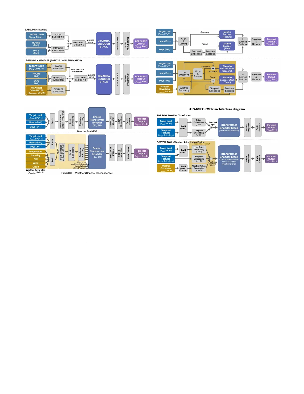
1 Benchmarking State Space Models, T ransformers, and Recurrent Networks for US Grid F orecasting Sunki Hong, Jisoo Lee, Member , IEEE , and Y uanyuan Shi, Member , IEEE Abstract —Selecting the right deep learning model for power grid f orecasting is challenging, as performance heavily depends on the data av ailable to the operator . This paper presents a com- prehensi ve benchmark of five modern neural architectur es—two state space models (PowerMamba, S-Mamba), two T ransformers (iT ransformer , PatchTST), and a traditional LSTM. W e evaluate these models on hourly electricity demand across six div erse US power grids for forecast windows between 24 and 168 hours. T o ensure a fair comparison, we adapt each model with specialized temporal processing and a modular layer that cleanly integrates weather cov ariates. Our results re veal that there is no single best model for all situations. When f orecasting using only historical load, P atchTST and the state space models pr ovide the highest accuracy . Howev er , when explicit weather data is added to the inputs, the rankings re verse: iT ransformer improves its accuracy three times more efficiently than PatchTST . By controlling for model size, we con- firm that this advantage stems from the architectur e’s inherent ability to mix inf ormation across different variables. Extending our evaluation to solar generation, wind power , and wholesale prices further demonstrates that model rankings depend on the for ecast task: PatchTST excels on highly rhythmic signals like solar , while state space models are better suited for the chaotic fluctuations of wind and price. Ultimately , this benchmark pro vides grid operators with actionable guidelines for selecting the optimal for ecasting architectur e based on their specific data en vironments. Index T erms —Load forecasting, benchmark, state space mod- els, T ransformers, deep learning, US grid operators I . I N T R O D U C T I O N S HOR T -TERM load forecasting (STLF) underpins elec- tricity grid operations, gov erning unit commitment and economic dispatch [1], [2]. Despite rapid architectural innov ation—from LSTMs to T ransformers to state space models (SSMs) [3]—most deep learning forecasting studies ev aluate on a handful of grids (typically 1–5). This limited scope makes it difficult to assess whether architectural adv an- tages generalize across the div erse characteristics of US grid operators [4]. This limitation is particularly pressing as US grids face increasing complexity . Behind-the-meter solar creates steep net-load ramps (the “duck curve”) in CAISO; extreme weather can trigger non-linear demand spikes in ERCO T ; and each ISO exhibits distinct load profiles shaped by regional climate, in- dustrial mix, and renew able penetration. Three model families S. Hong and J. Lee are with Gramm AI (e-mail: sunki@gramm.ai; jisoo@gramm.ai). Y . Y . Shi is with the Department of Electrical and Computer Engineering, Univ ersity of California San Diego, La Jolla, CA 92093 USA (e-mail: yyshi@ucsd.edu). Corresponding author: Jisoo Lee. currently compete—recurrent networks (LSTMs), T ransformer variants, and state space models—b ut whether their adv antages hold across US grid diversity and interact with weather cov ari- ate av ailability remains an open question. Practitioners need reliable guidance: which arc hitecture should they deploy for their specific grid? W e address this gap with a systematic benchmark of five neural architectures across six major US independent system operators. Using hourly load data from EIA-930, we e valuate each architecture under identical preprocessing, training, and ev aluation protocols across forecast windows from 24 to 168 hours, with additional analysis of weather feature integration. 1) US Grid Benchmark. W e conduct a comprehensi ve comparison of SSMs (Po werMamba, S-Mamba), T rans- formers (iTransformer , PatchTST), and an LSTM across six major US ISOs with consistent hyperparameters. PatchTST leads by outperforming on 15 of 30 ev al- uations (MAPE), followed by SSMs (14 of 30 com- bined). W e report MSE (%), MAPE (%), and signed- error tails ( P 0 . 5 /P 99 . 5 ) in an operator-by-windo w layout (Section V -B). 2) W eather Inte gration Benchmark. W e dev elop thermal- lag-aligned weather fusion strategies for each architec- ture and e v aluate all fi ve models across seven US grids at W = 24 . iT ransformer’ s cross-variate attention achiev es 3 × greater weather benefit than PatchTST’ s channel- independent design ( − 1 . 62 vs. − 0 . 52 percentage points av erage ∆ MAPE), re vealing that weather integration ef- fectiv eness is architecturally determined (Section V -C). 3) Multitype Generalization. W e extend the benchmark to solar generation, wind generation, wholesale price, and ancillary-service forecasting across US grids, show- ing that architectural rankings are task-dependent: PatchTST dominates intermittent signals while SSMs lead smoother signals (Section V -D). I I . B A C K G RO U N D A N D R E L AT E D W O R K A. Operational Role of Short-T erm Load F or ecasting Short-term load forecasting (STLF) predicts aggregate elec- tricity demand from hours to days ahead and is a core input to system operations [1], [2], [5]. US wholesale markets operate under a two-settlement structure—day-ahead clearing based on forecasted demand and real-time settlement of deviations [6]—with STLF feeding both stages. Security-constrained unit commitment (SCUC) and economic dispatch (SCED) rely directly on load forecasts, and operating reserve requirements 2 scale with expected forecast error [7]. Our benchmark win- dows (Section III-A) span the operational range from real-time dispatch (1–6 h) through day-ahead commitment (12–36 h) to resource adequacy planning (48–168 h). B. Deep Learning for T ime Series F orecasting Deep learning has largely displaced statistical methods (ARIMA, SVR) for short-term load forecasting [4], [8]. The power systems community has acti vely embraced deep neural networks to manage the increasing stochasticity of smart grids. Recent studies in premier venues like the IEEE T r ansactions on Smart Grid and IEEE T ransactions on P ower Systems hav e demonstrated the ef ficacy of deep learning across di- verse forecasting challenges. Innov ations include deep resid- ual networks [9], densely connected networks [10], pooling- based deep RNNs [11], and ensemble learning frameworks [12], [13] for deterministic structural forecasting. T o capture uncertainty , researchers ha ve proposed Bayesian deep learning [14], probabilistic multitask prediction models [15], transfer- learning frame works for masked behind-the-meter loads [16]– [18], collaborative multi-district approaches [19], and ad- vanced quantile-mixing methods [20]. While these studies hav e successfully introduced powerful bespoke architectures tailored to specific challenges (e.g., behind-the-meter solar, probabilistic limits), they often ev al- uate models on restricted datasets or a fe w isolated operators. Our work complements this rich literature by providing a sys- tematic, cross-architecture benchmark—ev aluating pure SSMs, T ransformers, and RNN paradigms on identical footing across six di verse US market operators and systematically quantifying how weather cov ariate inte gration interacts with each founda- tional architecture. Specifically , within the Transformer f amily , two multi variate strategies ha ve emerged: channel-independent patching [21] and cross-variate tokenization [22]. In parallel, state space models have brought linear-time complexity to sequence modeling [3], [23], challenging the quadratic scaling of T ransformers. LSTMs remain the most widely deplo yed class in operational settings [24], [25]. W e benchmark these pure architectural paradigms to establish their foundational behavior before they are blurred by hybrid designs (e.g., Mambaformer). While zero-shot foundation models (T imesFM [26], Chronos [27]) are emerging, this paper focuses on trained- from-scratch (TFS) architectures that can natively integrate grid-specific, delay-aligned weather covariates—a capability that current zero-shot models lack without extensi ve fine- tuning. Each paradigm has been e valuated on energy data, b ut rarely against each other under identical conditions. Po werMamba [28] benchmarked a bidirectional SSM on five US grids; S-Mamba [29] demonstrated SSM effecti veness on general multiv ariate benchmarks but was not e valuated on US grid data; PatchTST [21] established records on ETTh/ETTm datasets with limited grid di versity . Direct comparisons be- tween LSTMs and modern SSMs under production-like con- ditions are scarce, and systematic cross-architecture ev aluation of weather integration remains limited [1], [8], [30]. No prior work benchmarks SSM, Transformer , and RNN architectures across multiple US ISOs under identical protocols. Our bench- mark addresses these gaps: five models across six US grids (sev en for weather experiments), with architecture-matched weather integration and parameter-controlled comparisons to disentangle capacity from design. I I I . P R O B L E M F O R M U L AT I O N A N D D AT A C H A R A C T E R I S T I C S A. F orecast T ask Definition W e study system-level (balancing-authority aggregate) load forecasting rather than nodal or zonal forecasting. System- lev el forecasting is the primary input to SCUC/SCED and is the lev el at which ISOs report forecast accuracy . W e use EIA-930 hourly demand series [31], the only publicly av ail- able dataset pro viding consistent, hourly , multi-ISO load data across the US—making it uniquely suited for cross-operator benchmarking. Giv en a historical window of length L , the model predicts the next W steps: ˆ y t +1: t + W = f θ ( x t − L +1: t , z t − L +1: t ) , (1) where x is historical load and z denotes optional exogenous features (temporal embeddings and, when enabled, weather co- variates). This formulation supports two deployment-relev ant settings: load-only inference ( z = calendar context) and weather-augmented inference ( z includes meteorological co- variates). Comparing both settings clarifies when architectural advantages depend on exogenous information av ailability . Spe- cific values of L and W are defined in Section V -A. B. Signal Characteristics and Exog enous Drivers Grid load signals are multi-periodic and non-stationary . Strong daily (24-hour) and weekly (168-hour) cycles domi- nate, with typical peak-to-trough ratios of 1.3–1.7 × within a day and weekend loads 5–15% belo w weekday lev els. These periodicities coexist with trend shifts from weather, holidays, and economic activity . ISO-specific characteristics shape the forecasting challenge. CAISO exhibits the “duck curve”—midday net-load troughs from 30%+ solar penetration followed by steep e vening ramps. ERCO T is electrically isolated from the Eastern and W est- ern Interconnections, amplifying local weather sensitivity and reducing spatial load di versity . PJM and MISO, as the two largest US interconnections, benefit from geographic smooth- ing across div erse climate zones. ISO-NE is winter-peaking due to electric heating pre valence, unlike the summer-peaking pattern of most US grids. Non-stationarity is accelerating as behind-the-meter solar growth progressively reduces observ- able load during daylight hours, creating a div ergence between gross and net demand that complicates model training on historical data. W eather effects are mediated by a U-shaped temperature– load relationship: heating demand rises belo w ∼ 18 °C and cooling demand rises abov e it, with a comfort zone of minimal weather sensiti vity near the inflection point [1]. The response 3 is delayed by building thermal inertia—HV A C systems re- spond to temperature changes with 2–6 hour lags depending on building mass [30]. Solar irradiance and wind speed influence net demand more rapidly b ut with high intermittency . This motiv ates the lag-aware weather feature construction used in our weather experiments (Section V -C). I V . E V A L U A T E D A R C H I T E C T U R E S A. Model Ar chitectur es W e ev aluate fi ve models spanning three neural architecture families: two state space models representing different SSM design philosophies, two T ransformer variants with contrasting multiv ariate strategies, and an LSTM. S-Mamba: S-Mamba [29] represents a minimalist approach to state space modeling. It adapts the standard Mamba block for time series via a simple encoder -decoder structure: a linear projection embeds the input sequence into a hidden state D , followed by stacked Mamba layers. S-Mamba tests whether the core selecti ve state space mech- anism alone—without complex decomposition or attention— suffices for grid forecasting. Its design prioritizes computa- tional ef ficiency ( O ( n ) complexity), making it a candidate for resource-constrained edge deployment. P owerMamba: Po werMamba [28] addresses a specific lim- itation of standard SSMs: the difficulty of modeling disparate frequencies (e.g., long-term trend vs. daily seasonality) within a single state vector . PowerMamba introduces two critical innovations for energy data. First, Series Decomposition splits the input into "T rend" (low-frequenc y) and "Seasonal" (high-frequency) components, processing them via independent Mamba encoders. This ex- plicitly separates the duck curve drift from daily load cycles. Second, Bidir ectionality captures a holistic temporal context; unlike language modeling where causality is strict, time series analysis benefits from looking forward (e.g., smoothing), so PowerMamba processes sequences in both forward and back- ward directions. P atchTST : PatchTST [21] represents the channel- independent paradigm for T ransformer-based time series forecasting. Rather than tokenizing variables, PatchTST segments each uni variate channel into fixed-length patches and processes them with a shared T ransformer encoder . Channel independence means each v ariate shares the same Transformer weights, enabling efficient multi-channel processing without explicit cross-v ariable attention. This tests whether temporal pattern extraction alone suffices for accurate grid forecasting. iT r ansformer: The iT ransformer [22] challenges the stan- dard Transformer paradigm by tokenizing variables (embed- ding an entire time series v ariate as a single token) instead of time steps. Self-attention therefore computes correlations be- tween variables (e.g., Load vs. T emperature), explicitly mod- eling system-wide interdependencies. By design, this mech- anism requires multiple variates; with a single load variate, self-attention reduces to near-identity . LSTM: W e use a 2-layer bidirectional LSTM [24] with hidden dimension d = 256 as our recurrent baseline, yielding approximately 2.6M parameters at W = 48 . B. Ar chitectur e Adaptations for Grid F orecasting Direct application of generic time series models to load forecasting yields suboptimal results because these architec- tures lack two capabilities essential for grid operations: (1) awareness of temporal context —hourly and weekly demand cycles that dominate load profiles—and (2) the ability to selectively incorporate weather covariates whose influence on load is non-stationary and lagged. W e adapt each baseline with a shared set of domain-specific components while preserving the core architectural mechanism that each model is designed to test: T emporal embeddings. All sequence models (SSMs, LSTM) receiv e learnable hour-of-day ( R 24 × d/ 4 ) and day-of-week ( R 7 × d/ 4 ) embeddings, concatenated and projected to d model , then added to the input representation at each time step. PatchTST processes temporal conte xt implicitly through its patch structure; iT ransformer encodes hour and day as addi- tional v ariate tokens. These embeddings inject the strong 24h and 168h periodicities that characterize load without requiring the encoder to learn them from data alone. Bidir ectional encoding. SSMs and LSTM use bidirectional processing—separate forward and backward encoders whose outputs are fused via a learned linear projection. Crucially , bidirectional processing is applied strictly within the fixed- length lookback window ( L = 240 hours); no information from the forecast horizon W is accessible to the encoder . Unlike causal language models, load forecasting operates on a completed historical window where “future” context within that windo w is av ailable and informativ e. Bidirectional en- coding approximately doubles the encoder’ s parameter count relativ e to a unidirectional model, but captures both leading and lagging temporal relationships (e.g., a morning ramp informs the preceding ov ernight trough and vice versa). Attention-weighted pooling. Rather than mean-pooling the encoder’ s hidden states, SSMs and LSTM use a learned attention vector ( a = softmax ( W a H ) ) to produce a weighted summary c = P t a t h t . This allows the model to selec- tiv ely emphasize time steps most relev ant to the forecast (e.g., weighting recent ramp events more heavily than stable ov ernight periods). Modular weather inte gration. Each architecture recei ves weather covariates through a fusion mechanism matched to its inductiv e bias (detailed in Section IV -C). Critically , the weather integration layer is architecturally decoupled from the core encoder: it can be toggled on or of f by providing or withholding weather features at inference time, without re- training. This modularity enables the controlled experiments in Section V -C and the fair weather comparison in Section V -C. Impact on parameter counts. These adaptations increase parameter counts relative to original configurations (e.g., bidi- rectional encoding doubles SSM encoder parameters; weather cross-attention adds ∼ 330K per model). All counts reported reflect the full deployed configuration at W = 48 ; see the Supplementary Material for a per -model parameter breakdown. C. W eather-Inte grated Ar chitectur es The key challenge in weather fusion is respecting the building thermal lag described in Section III-B. W e developed 4 weather-inte grated variants of each architecture (Figure 1), all follo wing an encode-then-fuse pattern: the core encoder first processes load history and temporal features, then a secondary fusion layer incorporates meteorological context. This design ensures that the same encoder weights serve both load-only and weather-augmented inference, and that weather integration adds a fixed parameter overhead ( ∼ 0.3M for SSMs/LSTM, ∼ 0.7M for PatchTST), enabling fair cross- architecture comparison. Fusion Strate gies (Ar chitectur e-Matched): S-Mamba (Early Summation, F ig . 1a). By summing weather embeddings with load and temporal tokens prior to the BiMamba stack, all exogenous signals are projected into a unified d model dimen- sional space. The selectiv e state space mechanism then uses this fused representation to modulate its continuous transition matrices ( A , B , C ), allowing weather to directly gate the recurrent state updates at each timestep. P owerMamba (Pr e-Decomposition Fusion, F ig. 1b). W eather features are fused before the sequence is decomposed. Because meteorological events (e.g., prolonged heatwa ves) driv e both multi-day trend shifts and rapid sub-daily HV A C cycling, early fusion allo ws the moving-a verage decomposition module to appropriately route weather -induced variance into both the seasonal and trend BiMamba branches. P atchTST (Interleaved Cr oss-Attention, F ig. 1c). T o preserve PatchTST’ s core channel-independence inductive bias—which prev ents direct mixing of variates to a void ov erfitting—we patch load and weather channels independently . W e then insert a dedicated cross-attention sublayer where load patches query the weather patches. This permits the load representation to attend to relev ant meteorological context (e.g., a temperature spike) without entangling the self-attention dynamics of the load and weather streams. iT r ansformer (V ariate T okenization, F ig. 1d). iT ransformer is nativ ely designed to model cross-variate correlations. There- fore, each weather cov ariate is embedded as a distinct variate token sequence mapping the entire lookback window . These weather tokens are concatenated with load and temporal to- kens, exposing them directly to the global cross-variate atten- tion mechanism and enabling dynamic, pairwise correlation modeling (e.g., Load heavily attending to T emperature during summer peaks). LSTM (Early Concatenation). Gi ven the step-by-step recur - rent processing of the LSTM, weather features are concate- nated with load features at each timestep. This ensures the recurrent gating mechanisms (input, forget, and output gates) hav e simultaneous access to both the current demand and contemporaneous meteorological forcing, allo wing the hidden cell state to accumulate weather-dri ven momentum o ver time. V . E X P E R I M E N T S A N D R E S U LT S A. Experimental Setup Dataset and Splits: W e use hourly system-level load data from six major US independent system operators, sourced from the EIA-930 Hourly Electric Grid Monitor [31]. Each ISO pro vides approximately four years of hourly load data spanning 2022–2025. T able I summarizes the grids. T ABLE I: US grid operators in the benchmark. Peak load and primary operating characteristics. † SWPP is used in weather experiments only (Section V -C). ISO EIA ID Peak (GW) Characteristics CAISO EIA-CISO 47.1 High solar , duck curve ISO-NE EIA-ISNE 25.6 W eather-sensiti ve, winter peaks MISO EIA-MISO 127.1 Large, wind-rich PJM EIA-PJM 150.4 Largest US ISO SWPP EIA-SWPP 54.4 W ind-rich, central US † ERCO T EIA-ERCO 85.5 Isolated grid, extreme weather NYISO EIA-NYIS 32.1 Dense urban, summer peaks The six core ISOs span the operating characteristics de- scribed in Section III-B; SWPP is added for the weather- extension e xperiments. Context length is L = 240 hours (10 days), follo w- ing prior e vidence that long conte xt windo ws improve grid forecasting [28]. The main benchmark ev aluates prediction windows W = { 24 , 48 , 72 , 96 , 168 } . For weather integration analysis (Section V -C), we e valuate at W = 24 using fi ve meteorological cov ariates (temperature, humidity , wind speed, GHI, and cloud cov er; full list in the Supplementary Material) aligned with empirically deriv ed thermal lag parameters. Prepr ocessing. Load values are z-score normalized per grid using training-set statistics only (no information leakage). T emporal features (hour-of-day , day-of-week) are encoded as learnable embeddings (Section IV -B). Model Set and T r aining Pr otocol: W e benchmark five models from three neural architecture families: S-Mamba, PowerMamba, PatchTST , iT ransformer , and LSTM. Architec- ture definitions and grid-specific adaptations are described in Section IV -B and Section IV -C. Core model scales are fixed across operators for comparabil- ity ( d model = 256 for SSMs/PatchTST , d model = 512 for iTrans- former , and 2-layer bidirectional LSTM). Full architecture- by-architecture settings are reported in the Supplementary Material. All models are trained with AdamW optimizer (lr 10 − 3 , weight decay 10 − 4 ), OneCycleLR scheduler, up to 200 epochs with early stopping (patience 30 on validation MAPE). Each ( grid , model , W ) configuration trains independently from scratch with fixed seed (42). For the main benchmark we use a fixed chronological split (70%/15%/15%). Evaluation Metrics: Our primary metric is mean squared error , reported as a normalized percentage MSE (%) for cross- grid comparability , alongside mean absolute percentage error MAPE (%): MSE (%) = 100 ¯ y v u u t 1 n n X i =1 ( y i − ˆ y i ) 2 , (2) MAPE (%) = 100 n n X i =1     y i − ˆ y i y i     , (3) where ¯ y is the mean load of the test set. MSE (%) normalizes the root mean squared error by mean load, enabling direct comparison across grids of different scale. F or generation and price signals where actuals approach zero (e.g., nighttime 5 (a) S-Mamba: Early Fusion via Summation (b) PowerMamba: Summation into decomposed streams (c) PatchTST : Channel Fusion via Independent Patching (d) iT ransformer: W eather as additional tokens Fig. 1: W eather integration strategies. Each subfigure shows the baseline architecture (top) and its weather-integrated variant (bottom). (a) S-Mamba: early fusion by embedding-space summation. (b) PowerMamba: summation into decomposed streams. (c) PatchTST : channel fusion via independent patching. (d) iT ransformer: tokenization of weather variables for cross-variate attention. solar output), MAPE can be unstable. W e therefore report normalized MAE (nMAE) for non-load tasks: nMAE = 100 n ¯ y n X i =1 | y i − ˆ y i | , (4) ¯ y = 1 n n X i =1 | y i | . (5) T o characterize forecast-error tails, we use signed percentage error e i = 100( ˆ y i − y i ) / ( y i + ϵ ) (with ϵ = 10 − 6 ) and report the tail percentiles P 0 . 5 ( e ) and P 99 . 5 ( e ) . W alk-F orwar d Bac ktest: For weather integration analysis, we use a rolling-origin walk-forward backtesting protocol over Nov 2023–Nov 2025 (details in the Supplementary Material), aligning meteorological cov ariates to delayed HV A C response using empirically deriv ed thermal lag parameters. B. Load-Only P erformance Acr oss US Grids T able II presents the full benchmark across US operators and prediction windows; T able III reports the corresponding signed-error tails for all models; T able IV summarizes row- lev el wins and macro averages across all 30 (ISO , W ) ro ws. PatchTST emerges as the strongest load-only architecture, outperforming on the majority of ev aluations and achie ving the lowest average MAPE across all grid–horizon combinations (T able IV). SSMs are competitive, with particular strength on ISO-NE, PJM, and NYISO. Their O ( n ) inference complexity makes them attractiv e for operational deployment. In contrast, PatchTST leads on CAISO, MISO, and ERCO T at W = 48 , suggesting that grid-specific characteristics—discussed further in Section VI-B—interact with architectural inductiv e biases. As expected from Section IV, iTransformer’ s cross-variate attention de generates to near-identity with a single load variate, yielding the second-highest a verage error . This limitation establishes the baseline for the weather experiments in Sec- tion V -C, where additional variates restore the attention mech- anism. LSTM, despite 2.6M parameters, achieves the highest av erage MAPE, degrading markedly at longer horizons. For reference, published operational day-ahead MAPE val- ues are PJM ∼ 1 . 9% [32], ISO-NE ∼ 2 . 1% [33], and ERCO T ∼ 2 . 7% [34]. Our best 24-hour results approach these v alues for ERCO T but remain abov e PJM and ISO-NE targets. This performance gap reflects factors beyond architecture—weather forecasts, ensemble methods, human analyst correction, and more frequent retraining—that our controlled benchmark in- tentionally excludes to isolate architectural contrib ution. 6 T ABLE II: US ISO benchmark on load for ecasting. Results are reported per grid operator and prediction window ( W = 24 , 48 , 72 , 96 , 168 ) with fixed input length ( L = 240 ). For each model we report MSE (%) and MAPE (%) (lower is better). MSE (%) is normalized root mean squared error as a percentage of mean load. Best values per row are highlighted in bold . Full tail distribution metrics ( P 0 . 5 /P 99 . 5 ) for all models are reported separately in T able III. SSM T ransformer RNN ISO W PowerMamba S-Mamba iT ransformer P atchTST LSTM MSE MAPE MSE MAPE MSE MAPE MSE MAPE MSE MAPE (%) (%) (%) (%) (%) (%) (%) (%) (%) (%) CAISO 24 5.12 3.38 4.74 3.17 7.30 5.16 4.70 3.12 5.91 4.08 48 7.35 4.65 6.18 4.24 6.42 4.55 5.86 3.88 7.76 5.49 72 8.70 5.45 7.47 5.14 7.21 5.12 6.73 4.49 8.83 6.08 96 10.73 6.93 8.58 5.87 7.68 5.43 7.28 4.88 9.98 6.81 168 10.43 7.00 15.28 9.83 8.66 6.12 8.87 6.17 11.02 7.51 ISO-NE 24 8.64 5.86 8.84 5.95 9.42 6.41 8.80 6.06 9.60 6.74 48 11.67 7.77 11.96 8.00 12.45 8.29 11.77 8.01 12.52 8.58 72 13.16 8.93 13.34 9.05 14.41 9.56 13.55 9.13 19.06 14.02 96 14.24 9.83 14.38 9.99 15.47 10.34 14.37 9.72 17.11 11.89 168 15.08 10.58 15.18 10.61 16.33 11.18 15.29 10.55 19.68 14.24 MISO 24 3.50 2.38 3.46 2.33 4.10 2.88 3.56 2.37 4.37 2.97 48 5.18 3.51 5.65 3.62 5.44 3.77 5.22 3.46 6.20 4.20 72 6.47 4.36 6.78 4.44 6.46 4.47 6.32 4.25 6.98 4.68 96 7.54 5.10 7.33 5.00 7.16 4.94 7.10 4.83 8.83 6.13 168 8.44 6.05 8.88 6.37 8.53 5.98 8.25 5.66 9.19 6.28 PJM 24 4.72 3.14 4.51 2.97 5.16 3.46 5.00 3.21 5.47 3.59 48 6.59 4.33 6.29 4.19 6.94 4.60 7.19 4.62 6.94 4.73 72 8.31 5.36 7.84 5.32 8.22 5.44 8.78 5.73 9.08 6.00 96 8.59 5.73 8.88 6.08 9.04 6.00 9.64 6.36 16.09 10.66 168 10.91 6.93 10.47 7.45 10.37 7.00 10.41 6.99 16.39 11.12 ERCO T 24 4.76 2.98 4.92 3.17 7.47 5.26 4.65 2.85 5.24 3.40 48 6.13 4.00 6.17 4.01 8.45 5.95 6.07 3.87 6.54 4.23 72 6.79 4.39 6.96 4.60 9.02 6.32 6.78 4.38 7.19 4.68 96 7.39 4.88 7.47 5.01 7.67 5.07 7.21 4.71 7.79 5.17 168 8.38 5.70 8.27 5.69 8.51 5.72 7.74 5.13 8.70 5.98 NYISO 24 8.19 4.56 6.61 4.25 7.07 4.80 6.89 4.36 7.15 4.69 48 9.51 5.95 9.10 5.70 9.47 6.28 9.98 6.22 9.90 6.37 72 10.38 6.66 10.13 6.67 11.06 7.28 11.52 7.17 11.39 7.58 96 11.54 7.29 10.91 7.26 12.03 7.98 11.90 7.47 12.02 8.03 168 12.15 7.97 12.01 8.05 13.24 8.86 12.39 8.05 13.60 8.92 C. W eather Inte gration Acr oss Arc hitectures and Grids W e e valuate weather-integrated variants of all fiv e archi- tectures (Section IV -C) across se ven US grids at W = 24 , extending the benchmark set with SWPP . Unlike the fix ed-split protocol used for the main benchmark (Section V -B), weather experiments use the walk-forward backtest (described in the Supplementary Material) to approximate operational condi- tions; consequently , absolute MAPE v alues are not directly comparable between the two sections, though within-section deltas are valid. Each model uses its architecture-specific weather fusion strategy with thermal-lag alignment. Impor- tant assumption: weather cov ariates use observed (reanalysis) meteorological data rather than numerical weather prediction (NWP) forecasts, isolating neural-architecture differences from NWP forecast skill. Operational deployment would introduce additional error from imperfect weather forecasts, particularly at longer horizons. Three conditions are tested: none (load only), temporal (load + temporal embeddings as a matched- token control), and weather (load + weather co variates + temporal embeddings). This yields 105 experiments ( 7 × 5 × 3 ). T able V reports baseline and weather-inte grated MAPE for all model–grid combinations. T able VI summarizes the weather integration impact as ∆ MAPE (weather − none, in percentage points). W eather cov ariates improve all fiv e architectures on the majority of grids, but the magnitude of improv ement varies substantially by architecture (T able VI). iT ransformer benefits significantly more than PatchTST , with the gap widening on weather-sensiti ve grids (ERCOT and SWPP). This benefit gap is partly explained by iT ransformer’ s de- graded single-v ariate baseline: adding weather variates restores the multi-token attention that the architecture requires to function as designed. PatchTST’ s channel-independent base- line is already strong, lea ving less room for improv ement. A temporal-embedding control experiment supports this in- terpretation. T emporal-only tokens improve iT ransformer and LSTM, but have negligible effect on PatchTST , PowerMamba, and S-Mamba. This confirms that iT ransformer benefits from any additional tokens, not specifically from weather content. W ith weather features included, SSMs become the strongest models overall. S-Mamba achieves the best MAPE on SWPP , ERCO T , and NYISO, while PowerMamba leads on ISO-NE and MISO. iT ransformer outperforms on CAISO and ties PJM. Capacity-Contr olled Comparison: The weather benefit gap between iTransformer ( − 1 . 62 percentage points) and PatchTST ( − 0 . 52 percentage points) could reflect param- 7 T ABLE III: T ail distributions of f orecast errors. Signed percentage-error tails P 0 . 5 /P 99 . 5 for each model across grid operators and prediction windows. Negati ve P 0 . 5 indicates under-prediction; positive P 99 . 5 indicates over - prediction. PwrM.: PowerMamba; iTrnsf.: iT ransformer; PTST : PatchTST . Grid W PwrM. S-Mamba iT rnsf . PTST LSTM (%) (%) (%) (%) (%) CAISO 24 -14.1/13.4 -12.2/12.5 -17.1/19.8 -12.6/11.6 -15.9/14.2 48 -17.1/24.9 -14.3/18.1 -17.9/17.6 -15.3/15.8 -19.6/18.5 72 -21.0/29.7 -16.3/21.2 -19.5/19.7 -17.7/16.4 -21.6/19.4 96 -20.7/37.4 -18.5/25.1 -19.8/21.1 -18.4/17.8 -23.3/20.9 168 -21.4/29.5 -22.4/51.2 -20.9/23.1 -22.1/19.8 -23.0/33.3 ISO-NE 24 -18.7/34.3 -17.5/36.2 -21.0/35.7 -20.0/32.2 -20.3/36.9 48 -25.9/43.8 -24.1/50.5 -27.9/50.4 -26.8/41.5 -27.6/45.4 72 -26.8/51.0 -28.7/49.4 -32.3/57.9 -30.5/48.2 -40.0/48.0 96 -28.5/54.0 -29.8/52.1 -33.6/59.6 -31.0/51.5 -38.4/57.2 168 -32.3/52.7 -33.6/48.1 -34.6/57.7 -36.5/49.8 -41.5/46.7 MISO 24 -8.5/10.8 -8.7/10.6 -10.3/11.9 -9.6/11.0 -10.9/12.4 48 -13.2/15.1 -14.2/15.6 -13.7/16.4 -13.3/16.7 -16.6/16.0 72 -16.4/17.9 -17.5/19.6 -16.5/19.9 -14.8/19.9 -19.2/17.3 96 -19.1/19.8 -17.6/21.2 -18.2/21.9 -17.0/21.4 -19.3/21.5 168 -18.0/25.2 -19.1/25.3 -19.1/25.7 -19.3/23.7 -21.5/21.1 PJM 24 -11.8/13.0 -11.2/12.7 -12.7/15.2 -12.5/15.1 -13.7/14.2 48 -17.0/16.7 -15.7/17.7 -16.2/21.8 -16.9/23.2 -16.5/17.3 72 -22.0/20.9 -17.5/22.7 -18.3/26.9 -18.6/31.1 -21.4/20.3 96 -19.6/24.5 -19.2/25.2 -19.5/31.6 -21.9/33.6 -36.7/30.8 168 -30.0/21.9 -21.7/29.4 -23.1/32.5 -25.6/32.1 -34.0/34.8 ERCO T 24 -11.3/16.8 -11.0/17.2 -15.7/19.1 -12.0/16.2 -13.0/17.9 48 -13.6/20.2 -13.7/20.8 -17.7/22.2 -13.3/20.7 -16.0/20.9 72 -14.8/22.9 -14.9/23.4 -19.3/23.9 -15.1/22.1 -16.9/22.5 96 -16.4/22.6 -15.9/23.5 -17.8/24.9 -16.7/22.8 -18.2/23.3 168 -17.6/25.0 -15.9/28.2 -19.5/27.0 -17.5/26.1 -16.9/27.3 NYISO 24 -27.4/27.4 -13.9/24.6 -15.1/27.5 -16.0/27.3 -15.2/25.6 48 -21.6/40.3 -20.4/37.3 -20.8/37.5 -23.2/37.1 -22.7/34.4 72 -23.8/39.5 -22.3/37.6 -24.5/43.2 -27.2/40.1 -26.0/36.3 96 -30.6/39.7 -25.4/37.5 -26.5/44.9 -28.0/40.1 -27.7/37.3 168 -31.3/34.2 -29.8/37.1 -29.9/43.2 -30.4/36.1 -34.1/33.8 T ABLE IV: Benchmark scor ecard. MAPE (%) and MSE (%) averaged across the 30 (ISO , W ) rows. Row-le vel wins counted among the fiv e main architectures. Model Params MAPE (%) MSE (%) MSE Wins MAPE Wins PowerMamba 4.0M 5.72 7.62 7/30 7/30 S-Mamba 2.0M 5.80 7.58 9/30 7/30 iT ransformer 6.5M 6.14 7.95 2/30 1/30 PatchTST 2.0M 5.59 7.53 12/30 15/30 LSTM 2.6M 6.83 9.13 0/30 0/30 eter count dif ferences rather than architectural advantages: iT ransformer uses d model = 512 (6.5M parameters) while PatchTST uses d model = 256 (2.0M). T o disentangle capacity from architecture, we train two additional model variants. W e ev aluate Tier 1 ( d model = 512 ), comparing the paper-faithful iT ransformer (6.5M parameters) against a scaled PatchTST L ( d model = 512 , 9.84M parameters); and T ier 2 ( d model = 256 ), comparing a shrunk iTransformer S (2.44M parameters) against the paper-faithful PatchTST (2.0M parameters). Note that matching d model does not equalize total parameter counts because the architectures differ structurally: PatchTST’ s patch embedding, multi-head self-attention, and feed-forward lay- ers scale differently with d model than iTransformer’ s variate- tokenization and cross-variate attention. W e therefore match the hidden dimension—the primary capacity bottleneck—and report exact counts for transparenc y . Each v ariant is e valuated across all se ven grids un- der the same three conditions (none, temporal, weather), yielding 84 additional experiments. T able VII reports the ∆ MAPE (weather − none) for all four variants alongside the iT ransformer–P atchTST gap ( ∆ Gap) at each tier . The results confirm that the weather advantage is archi- tectural, not capacity-driven. Scaling P atchTST to d = 512 degrades its av erage ∆ MAPE, indicating that additional ca- pacity does not impro ve weather utilization in a channel- independent design. Con versely , shrinking iT ransformer to d = 256 preserves its weather benefit, demonstrating robust- ness to a parameter reduction. The gap is consistent across both tiers: iTransformer outperforms its capacity-matched PatchTST counterpart on the majority of grids at each tier (T able VII). ISO-NE is the only grid where PatchTST variants benefit more at both tiers. Grid-Level Determinants of W eather Benefit: The preceding sections establish that weather features help all architectures and that the benefit magnitude is architecturally determined. A natural follo w-up question is which grids benefit the most. The naïve hypothesis—that grids in extreme climates should benefit more—would suggest that temperature variability ( σ T ) predicts weather integration value. W e examine this across the sev en US grids by comparing each grid’ s av erage ∆ MAPE with σ T and baseline forecast difficulty . Figure 2 sho ws that temperature v ariability is necessary but not sufficient for weather benefit. Grids with low σ T (such as CAISO) gain little from weather features, while high- variability grids sho w larger but heterogeneous benefits. The interaction between climate variability and baseline difficulty determines the realized benefit. Low variability , low benefit. CAISO shows near-zero or positiv e ∆ MAPE across all five models, consistent with its mild Mediterranean climate where load patterns are highly predictable from temporal features alone. High variability , high benefit. ISO-NE and ERCO T exhibit the largest weather benefits, where heating- and cooling-driven demand creates weather-dependent variance that temporal pat- terns cannot capture. High variability , modest benefit. MISO has the highest temperature variability but the smallest weather benefit among the high-v ariability grids. Its low baseline MAPE indicates that spatial smoothing across its large footprint already re- duces weather-dri ven variance, leaving little residual signal for weather cov ariates to exploit. These patterns suggest a ceiling ef fect in which temperature variability determines the potential for weather-driv en load variance, but baseline forecast difficulty determines how much of that v ariance remains unexploited. When load-only models already achieve MAPE near 2% (MISO, PJM), temporal patterns capture most variance and weather cov ariates provide diminishing returns. W eather integration is most valuable where high climate v ariability coincides with high baseline 8 T ABLE V: W eather integration r esults: Load-only vs. W eather -integrated MAPE (%) acr oss 7 US grids ( W = 24 ). Bold marks the best MAPE per grid within each condition. ‘Load’ uses historical load only; ‘W eather’ adds meteorological cov ariates. All models use architecture-specific weather fusion (Section IV -C). iT ransformer PatchTST PowerMamba S-Mamba LSTM Grid Load W eather Load W eather Load W eather Load W eather Load W eather CAISO 5.16 3.19 3.12 3.20 3.38 3.51 3.17 3.62 4.08 3.71 ISO-NE 6.41 5.01 6.06 4.41 5.86 3.62 5.95 3.63 6.74 6.20 MISO 2.88 2.25 2.37 2.31 2.38 2.11 2.33 2.16 2.97 2.62 PJM 3.46 2.73 3.21 3.04 3.14 2.78 2.97 2.73 3.59 3.33 SWPP 5.94 3.32 3.47 3.21 3.50 3.18 3.43 3.11 4.37 3.70 ERCO T 5.26 2.39 2.85 2.05 2.98 2.09 3.17 1.96 3.40 3.37 NYISO 4.80 3.69 4.36 3.56 4.56 3.30 4.25 3.11 4.69 4.36 −4 −2 0 2 Δ MAPE (pp, weather − baseline) CAISO (6.4 °C) ERCOT (8.5 °C) NYISO (9.9 °C) PJM (10.0 °C) ISO -NE (10.1 °C) SWPP (10.6 °C) MISO (10.9 °C) ← Improved Worsened → −40 −20 0 20 Δ Error Range (pp, weather − baseline) ← Improved Worsened → iTransformer P atchTST PowerMamba S-Mamba LSTM Fig. 2: W eather integration impro ves accuracy and narrows the error range, with str onger effects on weather -sensitive grids. The plot illustrates the change in MAPE (left) and Error Range ( P 99 . 5 − P 0 . 5 , right) for fi ve neural architectures when transitioning from load-only to weather-inte grated forecasting ( W = 24 ). Negativ e values indicate improv ement. Grids are ordered by descending temperature v ariability ( σ T ). High-v ariability grids (e.g., ISO-NE, ERCO T) exhibit substantially lar ger improv ements in both mean accuracy and tail extremes compared to mild grids (e.g., CAISO). T ABLE VI: W eather integration impact ( ∆ MAPE, per - centage points). Negati ve values indicate improvement with weather cov ariates. Bold marks the largest improv ement per grid. Grid iT ransformer PatchTST PowerMamba S-Mamba LSTM CAISO -1.97 +0.08 +0.13 +0.45 -0.37 ISO-NE -1.40 -1.65 -2.24 -2.32 -0.54 MISO -0.63 -0.06 -0.27 -0.17 -0.35 PJM -0.73 -0.17 -0.36 -0.24 -0.26 SWPP -2.62 -0.26 -0.32 -0.32 -0.67 ERCO T -2.87 -0.80 -0.89 -1.21 -0.03 NYISO -1.11 -0.80 -1.26 -1.14 -0.33 A verag e -1.62 -0.52 -0.74 -0.71 -0.36 error—typically electrically isolated grids (ERCOT), smaller systems (SWPP), and weather-sensiti ve regions (ISO-NE). T ABLE VII: Parameter -controlled weather comparison. MAPE (%) for baseline (None) and weather-integrated (Wx) variants at matched d model sizes. ∆ is W eather − None (pp). Tier 1 ( d = 512 ) Tier 2 ( d = 256 ) Grid iTransformer PatchTST L ∆ Gap iTransformer S PatchTST ∆ Gap (6.44M) (9.84M) (2.44M) (1.77M) CAISO -1.97 +0.20 -2.17 -0.75 +0.08 -0.83 ISO-NE -1.40 -1.62 +0.22 -0.71 -1.65 +0.94 MISO -0.63 +0.13 -0.76 -2.49 -0.06 -2.43 PJM -0.73 -0.02 -0.71 -2.28 -0.17 -2.11 SWPP -2.62 -0.16 -2.46 -2.32 -0.26 -2.06 ERCO T -2.87 -0.56 -2.31 -1.96 -0.80 -1.16 NYISO -1.11 -0.67 -0.44 -0.72 -0.80 +0.08 D. Generalization Be yond Load T o test whether architectural rankings generalize beyond load, we extend the benchmark to solar generation (6 core ISOs), wind generation (7 grids: the 6 core ISOs plus SWPP), wholesale electricity price (4 grids: CAISO, ERCO T , NYISO, ISO-NE), and ERCOT ancillary services (4 types: RegUp, 9 RegDo wn, RRS, NonSpin)—totaling 21 grid–signal combina- tions, 5 models, and 2 conditions (none, weather) at W = 24 . Because MAPE di ver ges when actuals approach zero (e.g., nighttime solar), we use nMAE as the primary metric for all non-load tasks. T ABLE VIII: Multitype for ecasting scorecard: a verage nMAE (%) by signal type and model (no weather , W = 24 ). Bold marks the best model per ro w . Win counts reflect per-grid nMAE victories. † CAISO partial: 14 EIA-CISO logs lack nMAE (older metrics code). Signal T ype PatchTST S-Mamba PowerMamba iTransformer LSTM Solar 23.1 31.8 30.6 68.8 38.5 W ind 36.2 35.4 35.7 36.4 37.2 Price 30.9 27.5 34.1 60.4 37.5 Ancillary Svc. 79.3 119.9 139.1 597.2 131.5 nMAE Wins 11/18 5/18 2/18 0/18 0/18 T able VIII re veals that signal structure—rather than model family—determines the architectural ranking. PatchTST dom- inates signals with strong diurnal periodicity: solar and ancil- lary services, where its fixed-length patching aligns with 24- hour cycles. S-Mamba leads on signals with weaker periodic structure: wind and price, where continuous state dynamics better capture aperiodic dependencies. iTransformer’ s near- identity limitation (Section V -B) generalizes across all signal types, yielding poor performance on single-variate tasks. W eather benefit also v aries by task type in ways that differ from the load pattern. For wind, SSMs benefit most, reversing the load ranking where iTransformer gains the most. For price, iTransformer benefits strongly , recovering from its weak single-variate baseline. Solar shows mixed results: PatchTST and iT ransformer improve while SSMs slightly degrade. V I . D I S C U S S I O N A. Channel-Independent vs. Cr oss-V ariate Attention The load-only vs. weather-augmented ranking re versal traces to a fundamental architectural difference. iT ransformer’ s symmetric v ariate tokenization treats weather features as first- class tokens in the same attention space as load, enabling fine- grained load–weather interaction at each time step. PatchTST processes channels independently , so weather information can only influence load prediction indirectly through shared rep- resentations. This division explains the 3 × weather benefit gap (T able VI) and why it widens on weather-sensiti ve grids where hour -by-hour weather dynamics dri ve load v ariation. The capacity-controlled experiments (Section V -C) confirm this is architectural, not capacity-driv en. For practitioners, this suggests deploying PatchTST or SSMs for load-only forecasting, and switching to iTransformer or weather-aware SSM variants when weather forecasts are av ailable. B. Grid-Specific P erformance P atterns The benchmark rev eals a systematic split: PatchTST leads on CAISO, MISO, and ERCOT , while SSMs lead on ISO-NE, PJM, and NYISO. W e attribute this to the interaction between architectural inductiv e biases and load-profile regularity . PatchTST’ s fixed-length patches ( P = 16 hours) align well with grids dominated by strong, re gular diurnal pat- terns. CAISO’ s duck curve creates a stereotyped daily shape; MISO and ERCOT , as large summer-peaking systems, ex- hibit similarly predictable daily peaks. Patching con verts these regular structures into a small number of informati ve tokens. In contrast, PJM and NYISO serve dense, div erse load bases where daily patterns are modulated by irregular factors—subway schedules, commercial building occupancy , and div erse industrial loads. SSMs’ continuous state dynamics adapt to these irregularities through selecti ve gating, whereas PatchTST’ s fixed patch boundaries may straddle meaningful transitions. ISO-NE’ s winter -peaking profile, driv en by electric heating with weather-dependent intensity , similarly re wards the adaptiv e processing that SSMs provide. This interpretation is consistent with the multitype results (Section V -D), where PatchTST leads on signals with strong diurnal periodicity (solar) and SSMs lead on less periodic signals (wind, price). C. Implications for W eather Inte gration Three practical implications emerge for operators: Prioritize by baseline difficulty , not climate e xtremity . Oper- ators should in vest in weather integration on grids where load- only forecasts are weakest (ERCOT , ISO-NE), not where tem- perature swings are largest (MISO). Geographic load div ersity in large interconnections naturally smooths weather shocks, creating a ceiling ef fect that reduces the mar ginal v alue of explicit weather features. Match ar chitectur e to input availability . iT ransformer’ s single-variate weakness (avg 4.84% baseline) makes it unsuit- able for load-only deployment, but its cross-variate attention becomes the strongest weather utilization mechanism when cov ariates are available. This input-dependent ranking means operators should maintain different model configurations for different data-av ailability scenarios. W eather -aware SSMs combine accuracy with ef ficiency . S- Mamba and PowerMamba achiev e the best absolute MAPE on 5/7 grids with weather features while retaining O ( n ) inference complexity—making them attracti ve for real-time operational deployment where both accuracy and latency matter . D. Limitations Statistical r obustness. Results use a fixed random seed (42). While the large experiment count (30 grid–horizon pairs per model) provides a robust aggreg ate view , multi-seed e valuation would quantify per-grid variance. W e also do not perform formal significance tests (e.g., paired W ilcoxon signed-rank) on per-timestamp errors; formal testing would strengthen conclusions for rows with narrow margins. Benchmark cover age. The weather benchmark covers W = 24 only; extension to longer horizons is planned. W e do not include foundation models (Chronos [27], T imesFM [26]) or recent architectures (T imeMixer [35], hybrid Mamba- T ransformer models). The multitype benchmark (Section V -D) 10 should be considered preliminary for ancillary services, where only ERCO T data is av ailable. Err or decomposition and latency . W e report aggregate MAPE and tail percentiles but do not stratify errors by peak vs. off-peak periods, which would provide more operationally actionable guidance. W e also use parameter count rather than wall-clock inference time as the efficienc y metric; actual latency measurements would better characterize the O ( n ) vs. O ( n 2 ) distinction. Context length. W e fix L = 240 hours following Power - Mamba [28] but do not ablate this choice. Future work should ev aluate the accuracy–conte xt trade-off. V I I . C O N C L U S I O N W e benchmarked fiv e models—two SSMs, two T ransform- ers, and an LSTM—across six US ISOs, with weather inte- gration on sev en grids and multitype generalization to solar, wind, price, and ancillary-service forecasting. This systematic ev aluation yielded three ke y findings. First, no single architecture dominates; input av ailabil- ity determines the optimal choice. PatchTST and SSMs lead for load-only forecasting, but this ranking re verses when weather cov ariates are av ailable: cross-variate attention (iT ransformer) and weather-a ware SSMs become strongest. Parameter -controlled experiments confirm this rev ersal is ar- chitectural, not capacity-driven. Operators should select archi- tectures based on what inputs their pipeline provides. Second, weather inte gration v alue is predictable from grid characteristics. Baseline forecast difficulty—not climate extremity—determines how much weather features help. Iso- lated and smaller grids benefit most; lar ge interconnections with geographic load diversity show ceiling effects. This provides a simple heuristic for prioritizing weather integration in vestments. Third, architectural rankings are task-dependent. PatchTST’ s fixed-length patching excels on signals with strong diurnal periodicity (load on regular grids, solar), while SSMs’ adaptive state dynamics lead on less periodic signals (wind, price) and grids with irregular load patterns. This task–architecture interaction means that benchmarks on a single signal type cannot predict performance on others. These findings provide actionable, input-dependent de- ployment guidance. Beyond specific recommendations, the benchmark establishes a reproducible, multi-ISO e valuation framew ork that future work can extend with foundation models, longer forecast horizons, and richer exogenous fea- tures. Our configurations, trained checkpoints, and ev aluation code are publicly av ailable at https://github.com/gramm- ai/ grid- forecast- benchmark. D A TA A V A I L A B I L I T Y Hourly load data are publicly available from the U.S. Energy Information Administration via EIA-930 [31]. W eather covari- ates were obtained from Open-Meteo hourly weather prod- ucts. All preprocessing code, model configurations, trained checkpoints, and ev aluation scripts are av ailable at https: //github .com/gramm- ai/grid- forecast- benchmark. R E F E R E N C E S [1] T . Hong and S. Fan, “Probabilistic electric load forecasting: A tutorial revie w , ” International Journal of F orecasting , vol. 32, no. 3, pp. 914– 938, 2016. [2] F . A. Ahmad et al. , “Short-term load forecasting utilizing a combination model: A brief review , ” Results in Engineering , 2024. [3] A. Gu, K. Goel, and C. Ré, “Efficiently modeling long sequences with structured state spaces, ” in International Conference on Learning Repr esentations , 2022. [4] Q. Dong et al. , “Short-term electricity-load forecasting by deep learning: A comprehensiv e survey , ” arXiv pr eprint arXiv:2408.16202 , 2024. [5] X. Dong, L. Cao, Y . Shi, and S. Sun, “ A short-term po wer load forecasting method based on deep learning pipeline, ” in Pr oceedings of IEEE Sustainable P ower and Energy Confer ence . IEEE, 2024. [6] A. J. W ood, B. F . W ollenberg, and G. B. Sheblé, P ower Generation, Operation, and Contr ol , 3rd ed. Hoboken, NJ: John Wile y & Sons, 2014. [7] North American Electric Reliability Corporation, “Reliability guideline: Resource adequacy and operating reserve assessment, ” NERC, T ech. Rep., 2023, available at https://www .nerc.com/. [8] Y . Eren and I. B. Kucukdemiral, “ A comprehensiv e review on deep learning approaches for short-term load forecasting, ” Renewable and Sustainable Energy Re views , vol. 189, p. 114031, 2024. [9] K. Chen, K. Chen, Q. W ang, Z. He, J. Hu, and J. He, “Short-term load forecasting with deep residual networks, ” IEEE T ransactions on Smart Grid , vol. 10, no. 4, p. 3943–3952, Jul. 2019. [Online]. A vailable: http://dx.doi.org/10.1109/tsg.2018.2844307 [10] Z. Li, Y . Li, Y . Liu, P . W ang, R. Lu, and H. B. Gooi, “Deep learning based densely connected network for load forecasting, ” IEEE T ransactions on P ower Systems , vol. 36, no. 4, p. 2829–2840, Jul. 2021. [Online]. A v ailable: http://dx.doi.org/10.1109/tpwrs.2020.3048359 [11] H. Shi, M. Xu, and R. Li, “Deep learning for household load forecasting—a novel pooling deep rnn, ” IEEE T ransactions on Smart Grid , vol. 9, no. 5, p. 5271–5280, Sep. 2018. [Online]. A vailable: http://dx.doi.org/10.1109/tsg.2017.2686012 [12] H.-Y . Su and C.-C. Lai, “T oward improved load forecasting in smart grids: A robust deep ensemble learning framework, ” IEEE T ransactions on Smart Grid , vol. 15, no. 4, p. 4292–4296, Jul. 2024. [Online]. A vailable: http://dx.doi.org/10.1109/tsg.2024.3402011 [13] L. V on Krannichfeldt, Y . W ang, and G. Hug, “Online ensemble learning for load forecasting, ” IEEE T ransactions on P ower Systems , vol. 36, no. 1, p. 545–548, Jan. 2021. [Online]. A vailable: http://dx.doi.org/10.1109/tpwrs.2020.3036230 [14] M. Sun, T . Zhang, Y . W ang, G. Strbac, and C. Kang, “Using bayesian deep learning to capture uncertainty for residential net load forecasting, ” IEEE Tr ansactions on P ower Systems , vol. 35, no. 1, p. 188–201, Jan. 2020. [Online]. A vailable: http://dx.doi.org/10.1109/tpwrs.2019.2924294 [15] J. W ang, K. W ang, Z. Li, H. Lu, H. Jiang, and Q. Xing, “ A multitask integrated deep-learning probabilistic prediction for load forecasting, ” IEEE T ransactions on P ower Systems , vol. 39, no. 1, p. 1240–1250, Jan. 2024. [Online]. A vailable: http://dx.doi.org/10.1109/tpwrs.2023.3257353 [16] D. W u and W . Lin, “Efficient residential electric load forecasting via transfer learning and graph neural networks, ” IEEE T ransactions on Smart Grid , vol. 14, no. 3, p. 2423–2431, May 2023. [Online]. A vailable: http://dx.doi.org/10.1109/tsg.2022.3208211 [17] Z. Zhou, Y . Xu, and C. Ren, “ A transfer learning method for forecasting masked-load with behind-the-meter distrib uted energy resources, ” IEEE T ransactions on Smart Grid , vol. 13, no. 6, p. 4961–4964, Nov . 2022. [Online]. A v ailable: http://dx.doi.org/10.1109/tsg.2022.3204212 [18] Y . He, F . Luo, and G. Ranzi, “T ransferrable model-agnostic meta- learning for short-term household load forecasting with limited training data, ” IEEE Tr ansactions on P ower Systems , vol. 37, no. 4, p. 3177–3180, Jul. 2022. [Online]. A v ailable: http://dx.doi.org/10.1109/ tpwrs.2022.3169389 [19] H. Liu, X. Zhang, H. Sun, and M. Shahidehpour , “Boosted multi- task learning for inter-district collaborative load forecasting, ” IEEE T ransactions on Smart Grid , vol. 15, no. 1, p. 973–986, Jan. 2024. [Online]. A v ailable: http://dx.doi.org/10.1109/tsg.2023.3266342 [20] S. Ryu and Y . Y u, “Quantile-mix er: A novel deep learning approach for probabilistic short-term load forecasting, ” IEEE T ransactions on Smart Grid , vol. 15, no. 2, p. 2237–2250, Mar. 2024. [Online]. A vailable: http://dx.doi.org/10.1109/tsg.2023.3290180 [21] Y . Nie, N. H. Nguyen, P . Sinthong, and J. Kalagnanam, “ A time series is worth 64 words: Long-term forecasting with transformers, ” in International Conference on Learning Repr esentations , 2023. 11 [22] Y . Liu, T . Hu, H. Zhang, H. W u, S. W ang, L. Ma, and M. Long, “itrans- former: Inverted transformers are effecti ve for time series forecasting, ” in International Conference on Learning Repr esentations , 2024. [23] A. Gu and T . Dao, “Mamba: Linear-time sequence modeling with selectiv e state spaces, ” in Conference on Language Modeling , 2024. [24] S. Hochreiter and J. Schmidhuber, “Long short-term memory , ” Neural Computation , vol. 9, no. 8, pp. 1735–1780, 1997. [25] S. Bouktif, A. Fiaz, A. Ouni, and M. A. Serhani, “Optimal deep learning lstm model for electric load forecasting using feature selection and genetic algorithm: Comparison with machine learning approaches, ” Ener gies , vol. 13, p. 1633, 2020. [26] A. Das, W . K ong, R. Sen, and Y . Zhou, “ A decoder-only foundation model for time-series forecasting, ” arXiv preprint , 2024. [27] A. F . Ansari et al. , “Chronos: Learning the language of time series, ” arXiv preprint arXiv:2403.07815 , 2024. [28] A. Menati, F . Doudi, D. Kalathil, and L. Xie, “Powermamba: A deep state space model and comprehensi ve benchmark for time series prediction in electric power systems, ” arXiv preprint , 2024. [29] Z. W ang, F . Kong, S. Feng, M. W ang, X. Y ang, H. Zhao, D. W ang, and Y . Zhang, “Is mamba ef fective for time series forecasting?” arXiv pr eprint arXiv:2403.11144 , 2024. [30] J. E. Seem, “Dynamic modeling of buildings with thermal mass, ” ASHRAE T ransactions , vol. 113, no. 1, pp. 518–529, 2007. [31] U.S. Energy Information Administration, “Hourly Electric Grid Mon- itor (EIA-930), ” https://www .eia.go v/electricity/gridmonitor/, 2025, ac- cessed: 2025-11-01. [32] PJM Interconnection, “Forecasted vs. Actual Loads: Fall/W inter 2023– 2024, ” https://www .pjm.com/committees- and- groups/subcommittees/ las, 2024, load Analysis Subcommittee report, May 2024. [33] ISO New England, “Forecast Performance Report, ” https://www .iso- ne. com/, 2025, annual load forecast accuracy metrics. [34] ERCO T, “Mid-T erm Load Forecast Performance, ” https://www .ercot. com/, 2021, weather and Markets W orking Group presentation. [35] S. W ang, H. W u, X. Shi, T . Hu, H. Luo, L. Ma et al. , “T imemixer: Decomposable multiscale mixing for time series forecasting, ” in Inter- national Conference on Learning Repr esentations , 2024.