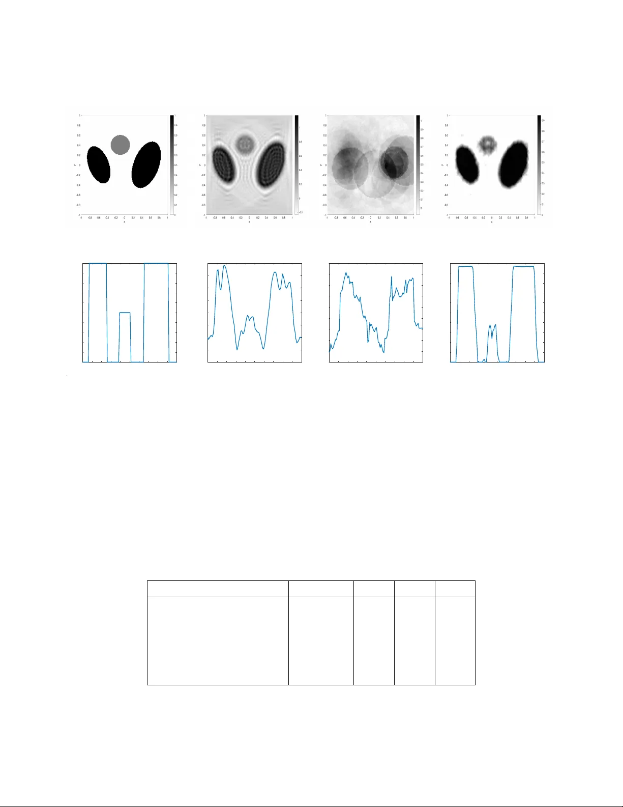
Photoacoustic tomography with time-dependent damping: Theoretical and a convolutional neural network-guided numerical inversion procedure

Photoacoustic tomograph y with time-dep enden t damping: Theoretical and a con v olutional neural net w ork-guided n umerical in v ersion pro cedure Sungh wan Mo on a , Anw esa Dey b , and Souvik Roy c a Departmen t of Mathematics, Kyungpo ok National Univ ersity , Daegu 41566, Republic of Korea b Departmen t of Mathematics, Univ ersit y of Utah, Salt Lake Cit y , UT 84112, USA c Departmen t of Mathematics, The Universit y of T exas at Arlington, Arlington, TX 76019, USA Abstract In photoacoustic tomograph y (P A T), a h ybrid imaging modality that is based on the acoustic detec- tion of optical absorption from biological tissue exp osed to a pulsed laser, a short pulse laser generates an initial pressure proportional to the absorbed optical energy , which then propagates acoustically and is measured on the b oundary . T o account for the signicant signal distortion caused by acoustic atten uation in biological tissue, w e mo del P A T in heterogeneous media using a damped wa v e equa- tion featuring spatially v arying sound sp eed and a time-dependent damping term. Under natural assumptions, we show that the initial pressure is uniquely determined by the b oundary measurements using a harmonic extension of the b oundary data with energy deca y . F or constan t damping, an ex- pansion in Dirichlet eigenfunctions of − c 2 ( x )∆ leads to an explicit series reconstruction form ula for the initial pressure. Finally , we develop a gradient free n umerical metho d based on the Pon try agin’s maxim um principle to provide a robust and computationally viable approach to image reconstruction in attenuating P A T. k eyw ords: W av e equation, time-dep enden t damping, photoacosutic tomograph y , optimization, in- v ersion MSCco des: 35R30, 35L05, 49J20, 49K20 1 In tro duction Optical tomography (OT) is a biomedical imaging mo dalit y that exploits the propagation of light in the near–infrared (NIR) sp ectral range to reconstruct the optical prop erties of biological media, such as tissues. Since malignan t tissue t ypically scatters ligh t less than healthy tissue, accurate recov ery of spatially v arying scattering and absorption co ecien ts is essen tial for reliable cancer diagnosis. Ho wev er, the inv erse problem in OT is sev erely ill–p osed and, in practice, often leads to reconstructions with p o or spatial resolution. T o o vercome these limitations and obtain high–delity maps of optical parameters, a v ariety of m ulti–physics imaging tec hniques, suc h as uorescence molecular tomograph y , confo cal dif- fuse tomography , single–photon photoacoustic tomography , t w o–photon photoacoustic tomograph y , and ultrasound–mo dulated optical tomograph y , hav e b een developed under the um brella of h ybrid OT meth- o ds (see, e.g., [4, 14, 19]). Among these, photoacoustic tomograph y (P A T) [18, 42, 44] has emerged as 1 one of the most prominent approaches owing to its wide range of biomedical applications. Consequen tly , the dev elopmen t of accurate and ecient computational models for image reconstruction in P A T is of considerable imp ortance. In P A T, a heterogeneous ob ject, typically biological tissue, is illuminated along its b oundary by short pulses of NIR ligh t. As photons propagate through the medium, a fraction of the optical energy is absorbed, causing localized heating and subsequent thermo elastic expansion of the tissue, while the remaining photons undergo multiple scattering even ts. After the illumination ceases, the tissue co ols and con tracts. This sequence of rapid expansion and con traction generates transien t pressure v ariations inside the ob ject, which in turn pro duce acoustic (ultrasound) w a ves through the photoacoustic eect [9]. These pressure w av es propagate out ward and are recorded b y ultrasound detectors positioned on (or near) the surface of the object. A coustic propagation in tissue occurs on microsecond time scales, whic h are roughly three orders of magnitude slow er than optical diusion. The core mathematical task in P A T is an in verse problem: reconstructing the initial pressure distribution, whic h is proportional to the absorb ed optical energy densit y , from the measured acoustic signals at the b oundary (see, for instance, [5, 7, 30, 45] and the references therein). Man y mathematical studies on P A T model the pressure eld by the standard w a ve equation with a v ariable sound sp eed; see, for instance, [22, 26, 28, 31, 32] and the references therein. Although such mo dels capture the nite–sp eed propagation and heterogeneity of sound sp eed reasonably well, they ne- glect the attenuation mechanisms that are intrinsic to biological tissue. In reality , as pressure wa v es tra vel through the medium, their amplitudes are gradually reduced due to absorption, scattering, and viscous losses. This attenuation can signicantly inuence the measured signals and, if not appropriately accoun ted for, may lead to systematic reconstruction artifacts and loss of resolution. T o address this issue, several attenuation mo dels hav e b een prop osed in the P A T literature [6, 16, 27, 29, 33], including frequency–p o w er–law mo dels, thermo–viscous mo dels, and more general conv olution–in–time formula- tions; the corresponding inv erse problems are t ypically more challenging and may suer from increased ill–p osedness. Moreov er, most of these mo dels are formulated under the simplifying assumption of a constan t sound sp eed. In this work, we fo cus on a time–dep enden t damp ed wa v e equation in P A T. Sp ecically , we consider the pressure eld p ( x , t ) as the solution to the Cauc hy problem ∂ 2 t p ( x , t ) + γ ( t ) ∂ t p ( x , t ) − c ( x ) 2 ∆ p ( x , t ) = 0 , ( x , t ) ∈ R n × [0 , ∞ ) , (1) where n ∈ N denotes the spatial dimension, with the initial data p ( x , 0) = p 0 ( x ) , ∂ t p ( x , 0) = 0 . (2) Here, c ( · ) denotes a spatially v arying sound sp eed and γ ( · ) > 0 is a smooth, strictly p ositiv e damping function that mo dels cumulativ e attenuation phenomena such as absorption and viscous losses. W e assume that the region of in terest Ω ⊂ R n is a b ounded domain with smo oth b oundary ∂ Ω and that the sound sp eed, the damping co ecient, and the initial data satisfy the assumptions (3) stated in Section 2. The measured data are given by the b oundary trace g ( y , t ) = p ( y , t )   ( y ,t ) ∈ ∂ Ω × [0 , ∞ ) . In this paper, we study how to reconstruct the initial pressure distribution p 0 , and hence the absorb ed optical energy density , inside Ω from the knowledge of g . 2 W e also note that, when the damping co ecien t in (1) dep ends only on space, γ = γ ( x ) , related in verse problems ha ve been studied in the literature [15, 23, 24, 36]. F or v ariable sound sp eed c ( · ) the in verse problem can b e treated by time–rev ersal based reconstruction/the Neumann series reconstruction [25, 34, 35, 43], and in [23] this approac h w as further extended to the case of spatially dep enden t damp- ing. In the context of multiw a ve imaging, Homan [24] and P alacios [36] analyzed damp ed w av e equations with spatially v arying attenuation and derived Neumann-series-t yp e reconstruction formulas under suit- able assumptions. How ev er, in the presence of time–dependent damping the underlying time–reversal symmetry is lost, and such time–reversal techniques no longer apply in a straightforw ard w ay . Our rst con tribution is an analytical study of the inv erse problem for the time–dependent damp ed w av e equation (1). Under assumptions of natural regularit y and b oundedness in c and γ , w e construct an auxiliary eld u satisfying homogeneous Dirichlet conditions on ∂ Ω whose energy deca ys in time. F ollowing the eigenfunction–expansion framew ork based on harmonic extension and Diric hlet eigenfunc- tions that was originally employ ed in the P A T con text b y Agrano vsky and Kuc hmen t [2], w e in tro duce the harmonic extension op erator E from ∂ Ω into Ω and expand the unkno wn eld in terms of Dirichlet eigenfunctions { ψ k } k ∈ N of the elliptic op erator − c ( x ) 2 ∆ . On this frame, w e establish that the initial pressure distribution p 0 is uniquely determined by the b oundary measurements g on ∂ Ω × [0 , ∞ ) , thus pro viding a uniqueness result for the P A T inv erse problem in the presence of a general time–dep endent damping term. Our second contribution is an explicit inv ersion pro cedure in the sp ecial but practically relev an t case where the damping co ecien t is constant, γ ( t ) = γ > 0 . Using the harmonic extension op erator and the unkno wn eld in terms of Dirichlet eigenfunctions, the damp ed wa v e equation is reduced to a family of decoupled second–order ordinary dieren tial equations for the co ecien ts. F or constant γ , these ODEs can b e solved explicitly , which yields closed–form expressions for the co ecien ts of u and, consequently , for p 0 − E g ( · , 0) in terms of time–conv olutions of the measured data g and its time deriv ativ es. This leads to an analytic series reconstruction formula for p 0 inside Ω in the weigh ted space L 2 (Ω , c − 2 ) . F or the numerical reconstruction of the initial pressure p 0 , w e aim to minimize a Tikhonov-t ype least-squares functional that incorporates data tting terms and sparsit y-promoting regularization terms. While the inclusion of nonsmo oth regularization signican tly enhances the method’s ability to pro duce sharp reconstructions, as demonstrated in [1, 39], it also necessitates adv anced optimization techniques suitable for nonsmo oth settings, tw o of whic h are pro ximal metho ds and semi-smo oth Newton (SSN) metho ds [8, 20, 21]. Ho w ever, implementing these approaches requires ev aluating the subgradien ts and Hessian of the optimization problem, which in volv es solving not only the state and adjoint equations but also tw o additional linearized systems. These requiremen ts, together with other implementation c hallenges, render these sc hemes demanding for practical use. T o address these c hallenges, w e use the sequen tial quadratic Hamiltonian (SQH) algorithm, whic h w as originally prop osed in [11, 12, 13] for nonsmo oth PDE-constrained optimal control problems, to our inv erse problem. The SQH metho d is grounded in the Pon try agin maxim um principle (PMP), a cornerstone of optimal con trol theory . W e are particularly motiv ated b y the SQH algorithm’s ease of implemen tation, strong eciency and robustness, and well-posedness as an iterative scheme [12, 13]. A distinctive feature of this iterative approac h is its reliance on a p oin twise optimization pro cedure. Suc h a scheme has b een recently used in context of tomographic inv erse problems arising in optical tomograph y [14, 38, 40, 41]. Ho wev er, since the SQH method is iterativ e, its p erformance dep ends hea vily on initial guesses. T raditional options are to either provide a sp ecied initial guess, lik e 0, or construct an appro ximate solution using some other algorithm and use that as the initial guess. It is w orthwhile to note that iterative algorithms lik e SQH w ork b etter if the structure of the initial guess resem bles the 3 structure of the true solution. One viable approac h w ould b e to use the time-reversal algorithm and obtain an approximation of p 0 , to be used as an initial guess. Ho w ever, ev en though the time-rev ersal algorithm migh t b e able to av oid appearance of spurious discontin uities or violate the underlying physics, due to the structure of the attenuated w av e equation, there will b e signicant damping, resulting in huge loss of contrast. On the other hand, conv olutional neural netw orks (CNNs) ha ve prov en highly eective for recov ering parameters in ill-p osed, PDE-constrained inv erse problems. The CNNs learns directly from data. Their data-driv en nature allo ws them to extract complex, problem-sp ecic features that would be dicult or ev en imp ossible to enco de analytically as explicit priors. Moreov er, CNNs are well suited for representing nonlinear relationships: by stac king con volution op erations, which are linear, with nonlinear activ ation functions, they build hierarc hical represen tations capable of appro ximating highly nonlinear mappings b et w een inputs and outputs. This interpla y of lay ered con v olutions and nonlinear activ ations enables CNNs to mo del in tricate structures that arise in challenging inv erse problems. F urthermore, unlike clas- sical optimization-based approaches, where regularization must b e in tro duced explicitly through p enalt y terms such as L 2 , L 1 , or Tikhonov regularization, CNNs em b ed regularization implicitly within their arc hitecture and training dynamics. Ho wev er, one ma jor drawbac k of CNN (or in general any traditional deep learning algorithm) is the inabilit y to incorp orate the underlying ph ysical structure of the problem and relies on training with a h uge dataset to pro vide meaningful inference, especially for complex in verse problems that usually appear with PDEs. There hav e been some progress made in the eld of machine learning through the dev elopmen t of physics-informed neural netw orks (PINN), but it still struggles to nd a balance b et ween learning patterns from data and satisfying ph ysical constraints. Thus, the output of CNN, in general, can suer from spurious artifacts. In an attempt to circumv en t this issue, we combine the adv an tages of time-rev ersal and CNN to c ho ose a initial guess of our SQH as the sum of the tw o outputs. This ensures that the initial guess preserv es some information of the discon tinuities present as well as provide b etter starting con trast. As w e will note in the results in Section 4, such a choice of initial guess guides the SQH algorithm to provide sup erior contrast and resolution reconstructions. The remainder of the pap er is organized as follows. In Section 2, w e presen t the analytical frame- w ork for the damped w a ve equation, including well–posedness and decay estimates, and w e derive the uniqueness result for the initial pressure as w ell as an explicit in version formula in the case of constant damping. In Section 3, we introduce the optimization framework for solving the initial pressure nu- merically . The framew ork comprises of a cost functional with data-tting and regularization terms. W e c haracterize the minimizer using the PMP , and describ e the SQH–based reconstruction algorithm, guided b y an initial guess obtained using a CNN, for the numerical PMP implemen tation along with results for the con v ergence of the algorithm. In Section 4, w e discuss the results of the reconstruction with our prop osed algorithm and compare our outputs with the time-rev ersal algorithm, both qualitativ ely and quan titatively . W e conclude the pap er with a section of conclusions. 2 Analysis of the damp ed w av e mo del In this section w e study the Cauch y problem (1)–(2) introduced in Section 1. Throughout the pap er w e imp ose the follo wing standing assumptions on γ , c , p 0 , and the b ounded domain Ω ⊂ R n with smo oth 4 b oundary ∂ Ω : for ν ∈ N , ν > n/ 2 + 1 , • γ ( · ) ∈ C ν +1 ([0 , ∞ )) with 0 < γ m ≤ γ ( t ) ≤ γ M , • c ( · ) ∈ C ν +1 ( R n ) with 0 < c m ≤ c ( x ) ≤ c M , • p 0 ∈ H ν ( R n ) with compact supp ort , • Ω ⊂ R n is an op en and b ounded domain with smo oth b oundary ∂ Ω . (3) W e notice that every scalar h yp erb olic equation of second order can b e transformed into a symmetric h yp erb olic system (see [37, page 21]). Hence b y Theorem 3.3 in [37], the initial problem (1) with p ( x , 0) = p 0 ( x ) , ∂ t p ( x , 0) = 0 under assumption (3) has a unique solution p ∈ C 2 ([0 , ∞ ) × R n ) and p ∈ C 1 ([0 , ∞ ); H ν ( R n ) ∩ C 2 ([0 , ∞ ); H ν − 1 ( R n )) , where H ν ( R n ) , ν ∈ R is the Sob olev space. Let E denote the harmonic extension operator from ∂ Ω to Ω , that is, the operator which pro duces a harmonic function E ϕ in Ω for giv en Diric hlet data ϕ on ∂ Ω . By standard regularity theory , E is con tinuous from H s ( ∂ Ω) to H s +1 / 2 (Ω) for an y s > 0 . Hence w e can rewrite (1) in terms of u = p − E g as follo ws: ∂ 2 t u ( x , t ) + γ ( t ) ∂ t u ( x , t ) − c ( x ) 2 ∆ u ( x , t ) = − G γ ( x , t ) for ( x , t ) ∈ Ω × [0 , ∞ ) u ( x , 0) = p 0 ( x ) − E g ( x , 0) and ∂ t u ( x , 0) = 0 for x ∈ Ω u ( y , t ) = 0 ( y , t ) ∈ ∂ Ω × [0 , ∞ ) , (4) where G γ ( x , t ) = E ( ∂ 2 t g )( x , t ) + γ ( t ) E ( ∂ t g )( x , t ) . Let { λ 2 k , ψ k } ∞ k =1 b e the eigen v alues and an associated orthonormal basis of eigenfunctions of the op erator − c ( x ) 2 ∆ with Dirichlet b oundary conditions, where λ k > 0 for all k . W e use the notation f k := h f , ψ k i , u k ( t ) := h u ( · , t ) , ψ k i , and G γ ,k ( t ) := h G γ ( · , t ) , ψ k i for the F ourier co ecien ts of f and u with resp ect to { ψ k } . Here h· , ·i denotes the inner pro duct in L 2 (Ω , c − 2 ) . Theorem 1. Under assumptions (3) , the initial function p 0 ( x ) − E g ( x , 0) c an b e uniquely determine d fr om E g ( x , t ) . F urthermor e, p 0 ( x ) c an b e uniquely determine d fr om g . T o establish the abov e uniqueness result and to prepare for an explicit reconstruction form ula, we expand the solution in the eigenbasis of the operator − c ( x ) 2 ∆ and study the time evolution of the corresp onding mo dal co ecien ts. The follo wing lemma pro vides that (4) satises these co ecien ts. Lemma 2. If for any k ∈ N , u k satises u ′′ k ( t ) + γ ( t ) u ′ k ( t ) + λ 2 k u k ( t ) = − G γ ,k ( t ) , (5) then L 2 (Ω , c − 2 ) -c onver gent series u = P u k ψ k satises the PDE in (4). Pr o of. F or any k ∈ N , let us consider Z Ω ∆ x u ( x , t ) ψ k ( x )d x = Z Ω u ( x , t )∆ x ψ k ( x )d x + Z ∂ Ω ∂ ν u ( y , t ) ψ k ( y ) − u ( y , t ) ∂ ν ψ k ( y )d s ( y ) = − Z Ω u ( x , t ) λ 2 k ψ k ( x ) c ( x ) − 2 d x , 5 where ∂ ν is the normal deriv ative on ∂ Ω , d s ( y ) denotes the surface measure on ∂ Ω and z , z ∈ C , is the complex conjugate of z . Here in the rst equality , w e used the Green’s theorem and we used the fact that u and ψ k in ∂ Ω are equal to 0 in the second equalit y . Multiplying the PDE in (4) b y ψ k and integrating o ver Ω with w eight c ( x ) − 2 , w e ha ve − G γ ,k ( t ) = Z Ω { ( ∂ 2 t + γ ( t ) ∂ t − c ( x ) 2 ∆ x ) u ( x , t ) } ψ k ( x ) c ( x ) − 2 d x = Z Ω { ( ∂ 2 t + γ ( t ) ∂ t + λ 2 k ) u ( x , t ) } ψ k ( x ) c ( x ) − 2 d x . Hence if for an y k ∈ N u k satises (5), then by the completeness of ψ k in L 2 (Ω , c − 2 ) L 2 (Ω , c − 2 ) -con vergen t series u satises the PDE in (4). T o prov e Theorem, we need the follo wing prop osition: Prop osition 3. Under assumptions (3) , ther e exists a unique glob al solution u of (4) such that lim t →∞ u ( x , t ) = lim t →∞ ∂ t u ( x , t ) = 0 for a.e. x ∈ Ω . (6) Pr o of. Let us start with energy function: E total ,u ( t ) = 1 2 Z Ω  c ( x ) − 2 | ∂ t u ( x , t ) | 2 + |∇ u ( x , t ) | 2  d x . Multiplying the PDE in (4) by ∂ t u and integrating ov er Ω , we obtain: Z Ω c ( x ) − 2 ∂ 2 t u ( x , t ) ∂ t u ( x , t )d x + Z Ω γ ( t ) c ( x ) 2 | ∂ t u ( x , t ) | 2 d x − Z Ω ∆ u ( x , t ) ∂ t u ( x , t )d x = − Z Ω c ( x ) − 2 G γ ( x , t ) ∂ t u ( x , t )d x . With Green’s theorem Z Ω ∇ u ( x ) · ∇ v ( x )d x = − Z Ω u ( x )∆ v ( x )d x + Z ∂ Ω u ( y ) ∂ ν v ( y )d s ( y ) , (7) this giv es: d d t E total ,u ( t ) + Z Ω γ ( t ) c ( x ) 2 | ∂ t u ( x , t ) | 2 d x = − Z Ω c ( x ) − 2 G γ ( x , t ) ∂ t u ( x , t )d x . and th us with Y oung’s inequality , w e hav e d d t E total ,u ( t ) + Z Ω γ ( t ) c ( x ) 2 | ∂ t u ( x , t ) | 2 d x ≤       Z Ω c ( x ) − 2 G γ ( x , t ) ∂ t u ( x , t )d x       ≤ 1 2 Z Ω γ ( t ) c ( x ) 2 | ∂ t u ( x , t ) | 2 d x + 1 2 Z Ω 1 γ ( t ) c ( x ) 2 | G γ ( x , t ) | 2 d x . 6 It can b e written as d d t E total ,u ( t ) ≤ d d t E total ,u ( t ) + 1 2 Z Ω γ ( t ) c ( x ) 2 | ∂ t u ( x , t ) | 2 d x ≤ 1 2 Z Ω 1 γ ( t ) c ( x ) 2 | G γ ( x , t ) | 2 d x . (8) F or any t ≥ 0 , integrating from 0 to t gives E total ,u ( t ) ≤ E total ,u (0) + 1 2 t Z 0 Z Ω 1 γ ( τ ) c ( x ) 2 | G γ ( x , τ ) | 2 d x d τ . (9) Lemma 4. F or the solution p of (1) and g = p | ∂ Ω × [0 , ∞ ) with the assumptions (3), we have E ∂ 2 t g ∈ L 2 (Ω × [0 , ∞ )) and E ∂ t g ∈ L 2 (Ω × [0 , ∞ )) . By Lemma 4, we hav e ∞ Z 0 Z Ω 1 γ ( t ) c ( x ) 2 | G γ ( x , t ) | 2 d x d t < ∞ , (10) and thus the integral on the right-hand side of (9) is nite. Hence E total ,u ( t ) remains b ounded and thus the solution u is global. Again in tegrating (8) from 0 to T gives E total ,u ( T ) + 1 2 T Z 0 Z Ω γ ( t ) c ( x ) 2 | ∂ t u ( x , t ) | 2 d x d t ≤ E total ,u (0) + 1 2 T Z 0 Z Ω 1 γ ( t ) c ( x ) 2 | G γ ( x , τ ) | 2 d x d τ . and th us ∞ Z 0 Z Ω γ ( t ) c ( x ) 2 | ∂ t u ( x , t ) | 2 d x d t < ∞ and th us for a.e. xed x ∈ Ω , ∂ t u ( x , t ) → 0 as t → ∞ . No w we sho w that for a.e. x ∈ Ω , u ( x , t ) → 0 as t → ∞ . Since lim t →∞ ∂ t u ( x , t ) = 0 , there is a function u ∞ on R n suc h that u ( x , t ) → u ∞ ( x ) . Then from (4) and lim t →∞ G γ ( x , t ) = 0 (b y (10)), we ha ve c ( x )∆ u ∞ ( x ) = 0 and u ∞ | ∂ Ω = 0 . Therefore w e ha ve u ∞ = 0 by strong maximum principle in [17, Chapter 6] and th us lim t →∞ u ( x , t ) = 0 . The uniqueness of u follows from (9) and the uniqueness of the solution p . It remains to prov e Lemma 4: Pr o of of L emma 4. Now consider the following energy function: for D α x = ∂ α 1 x 1 ∂ α 2 x 2 · · · ∂ α n x n , α = ( α 1 , α 2 , · · · , α n ) ∈ N ∪ { 0 } and | α | = P n i =1 α i ≤ 1 , E α total ,p ( t ) = 1 2 Z R n  c ( x ) − 2 | ∂ t D α x p ( x , t ) | 2 + |∇ D α x p ( x , t ) | 2  d x + t Z 0 Z R n F α ( x , τ ) D α x ∂ τ p ( x , τ )d x d τ , 7 where F α ( x , t ) = [ D α x , c ( x ) − 2 ]( ∂ 2 t p ( x , t ) + γ ( t ) ∂ t p ( x , t )) and [ A, B ] = AB − B A is comm uter. Dieren- tiating and using the PDE in (1) with Green’s Theorem (7) and compactness of p ([3, Chapter 7.4]) yields d d t E α total ,p ( t ) = − Z R n γ ( t ) c ( x ) 2 | ∂ t D α x p ( x , t ) | 2 d x ≤ 0 . (11) In tegrating (11) in time gives ∞ Z 0 Z R n γ ( t ) c ( x ) 2 | ∂ t D α x p ( x , t ) | 2 d x d t ≤ 2 E α total ,p (0) < ∞ , whic h implies ∂ t p ∈ L 2 ([0 , ∞ ); H 1 ( R n )) with assumption (3). By T race Theorem [17, Chapter 5] and the b oundedness of the harmonic extension op erator E : H s ( ∂ Ω) → H s + 1 2 (Ω) , we ha ve ∂ t g ∈ L 2 ( ∂ Ω × [0 , ∞ )) and || E ∂ t g ( · , t ) || L 2 (Ω) ≤ || E ∂ t g ( · , t ) || H 1 2 (Ω) ≤ C || ∂ t g ( · , t ) || H 0 ( ∂ Ω) , whic h implies E ∂ t g ∈ L 2 (Ω × [0 , ∞ )) . Similarly , considering the following energy functional E α high ,p ( t ) = 1 2 Z R n  c ( x ) − 2 | ∂ 2 t D α x p ( x , t ) | 2 + |∇ ∂ t D α x p ( x , t ) | 2  d x + t Z 0 Z R n  γ ′ ( τ ) c ( x ) 2 ∂ τ D α x p ( x , τ ) + ∂ τ F α ( x , τ )  ∂ 2 τ D α x p ( x , τ ) d x d τ , w e hav e d d t E high ,p ( t ) = − Z R n γ ( t ) c ( x ) 2 | ∂ 2 t D α x p ( x , t ) | 2 d x ≤ 0 . Notice that from (1) with assumptions (3), ∂ 2 t D α x p ( x , 0) ∈ L 2 ( R n ) and ∂ t D α x p ( x , 0) = 0 and thus ∞ Z 0 Z R n γ ( t ) c ( x ) 2 | ∂ 2 t D α x p ( x , t ) | 2 d x d t ≤ 2 E α high ,p (0) < ∞ . Hence w e hav e ∂ 2 t p ∈ L 2 ([0 , ∞ ); H 1 ( R n )) . Again b y T race Theorem [17, Chapter 5], and the b oundedness of the harmonic extension op erator, we hav e E ∂ 2 t g ∈ L 2 (Ω × [0 , ∞ )) . No w we are ready to prov e Theorem 1: 8 Pr o of of The or em 1. Let us consider the solutions ˜ u k of (5) with lim t →∞ ˜ u k ( t ) = lim t →∞ ˜ u ′ k ( t ) = 0 (12) The solution ˜ u k are determined by only G γ ,k (indep enden t on p 0 ). On the other hand, since the F ourier co ecien t u k of the solution u of (4) with initial and b oundary v alues (5) satises u k , u ′ k → 0 as t → ∞ , w e hav e u k = ˜ u k b y uniqueness of ODE solution. Hence p 0 can b e uniquely determined from ˜ u k and th us G γ ,k . By strong maximum principle in [17], E g is unique and thus we hav e our assertion. 2.1 Constan t damping In the sp ecial case where γ is constant, w e can deriv e an explicit in version pro cedure. Theorem 5. L et B k, ± = ( − γ ± A k ) / 2 and A k = ( γ 2 − 4 λ 2 k ) 1 / 2 . Then the series u ( x , t ) = P k ∈ N u k ( t ) ψ k ( x ) c onver ges in L 2 (Ω , c − 2 ) and its sum is a solution of (4) with the assumptions (3), wher e u k ( t ) = A − 1 k ∞ Z t  e B k, + ( t − τ ) − e B k, − ( t − τ )  G γ ,k ( τ ) d τ . Mor e over, the initial pr essur e p 0 c an b e r e c onstructe d as p 0 ( x ) = E g ( x , 0) + X k ∈ N A − 1 k ∞ Z 0 ( e − B k, + τ − e − B k, − τ ) G γ ,k ( τ )d τ ψ k ( x ) . Pr o of. T o chec k that u k is a solution of (5), we consider u ′ k and u ′′ k : u ′ k ( t ) = A − 1 k ∞ Z t ( B k, + e B k, + ( t − τ ) − B k, − e B k, − ( t − τ ) ) G γ ,k ( τ )d τ and u ′′ k ( t ) = − G γ ,k ( t ) + A − 1 k ∞ Z t ( B 2 k, + e B k, + ( t − τ ) − B 2 k, − e B k, − ( t − τ ) ) G γ ,k ( τ )d τ . Then using the fact that ( B k, ± ) 2 + γ B k, ± + λ 2 k = 0 , we hav e u k satises (5). All in all, u ( x , t ) = P u k ( t ) ψ k ( x ) satises the PDE in (4) with lim t →∞ u k ( t ) = lim t →∞ ∂ t u k ( t ) = 0 for any x ∈ Ω , k ∈ N . By uniqueness of the solution, we ha ve that u is the solution of (4). W e now eliminate the explicit app earance of the extension op erator E : G γ ,k ( t ) = Z Ω G γ ( x , t ) ψ k ( x ) c ( x ) − 2 d x = λ − 2 k Z Ω G γ ( x , t )∆ x ψ k ( x )d x = λ − 2 k Z ∂ Ω ( ∂ 2 t g ( y , t ) + γ ( y ) ∂ t g ( y , t )) ∂ ν ψ k ( y )d s ( y ) , 9 where w e used Green’s theorem, harmonicity of E g and ψ k = 0 on ∂ Ω , again. Similarly , w e hav e E g ( x , 0) = X k λ − 2 k Z ∂ Ω g ( y , 0) ∂ ν ψ k ( y )d s ( y ) ψ k ( x ) , in L 2 (Ω , c − 2 ) sense. Corollary 6. Under assumptions (3) , the initial function p 0 inside Ω c an b e r e c onstructe d fr om the data g in (1) as the fol lowing L 2 (Ω , c − 2 ) -c onver gent series: p 0 ( x ) = X k λ − 2 k p 0 ,k ψ k ( x ) , wher e p 0 ,k = Z ∂ Ω g ( y , 0) ∂ ν ψ k ( y )d y + A − 1 k ∞ Z 0 Z ∂ Ω ( e − B k, + t − e − B k, − t )( ∂ 2 t g ( y , t ) + γ ( y ) ∂ t g ( y , t )) ∂ ν ψ k ( y )d s ( y )d t, wher e d s ( y ) denotes the surfac e me asur e on ∂ Ω , again. 3 Numerical inv ersion pro cedure T o solv e for p 0 ( x ) given observ ation function g ( x , t ) on the observ ation domain ∂ Ω , w e consider the follo wing optimization problem: min p 0 ∈ P ad J ( p 0 , p ) := 1 2 T Z 0 Z ∂ Ω ( p ( x , t ) − g ( x , t )) 2 d s ( x )d t + α 2 Z Ω | p 0 ( x ) | 2 d x + β Z Ω | p 0 ( x ) | d x suc h that ∂ 2 t p ( x , t ) + γ ( t ) ∂ t p ( x , t ) − c ( x ) 2 ∆ p ( x , t ) = 0 , ( x , t ) ∈ R n × (0 , T ) , p ( x , 0) = p 0 ( x ) , x ∈ R n , ∂ t p ( x , 0) = 0 , x ∈ R n , (13) where p 0 ∈ P ad = { L 2 (Ω) : 0 ≤ p l ≤ p 0 ( x ) ≤ p r } . Here the rst term represents the standard least-squares data tting term, and the last tw o terms represent the L 2 − L 1 regularization term, with α, β > 0 , that has the ability to reconstruct sparsity patterns in p 0 ( x ) . W e rst remark that since the functional J is con v ex with respect to p 0 since the atten uated wa v e equation is a linear function of p 0 . Thus, there is exists a solution pair ( p ∗ 0 , p ∗ ) to the minimization problem (13). T o c haracterize the solutions of (13), w e use the framework of the Pon try agin’s maximum principle (PMP). F or this purp ose, we formulate the follo wing Hamiltonian function: H ( x , p 0 ( x ) , q ( x , :)) = α 2 | p 0 ( x ) | 2 + β | p 0 ( x ) | + p 0 ( x )[ ∂ t q ( x , 0) − γ (0) q ( x , 0)] , x ∈ Ω , (14) 10 where q ( x , t ) solv es the following adjoin t equation ∂ 2 t q ( x , t ) − ∂ t [ γ ( t ) q ( x , t )] − ∆[ c ( x ) 2 q ( x , t )] = − [ p ( x , t ) − g ( x , t )] χ ∂ Ω , ( x , t ) ∈ R n × (0 , T ) q ( x , T ) = 0 , x ∈ R n , ∂ t q ( x , T ) = 0 , x ∈ R n . (15) W e remark that the spatial domain for x in the denition of H is chosen to b e Ω , corresponding to the region of interest. Then, we hav e the following c haracterization of the optimal control through the PMP: Theorem 7. The optimal initial c ondition and adjoint ( p ∗ 0 , q ∗ ) satises the fol lowing PMP criterion H ( x , p ∗ 0 ( x ) , q ∗ ( x , :)) = min v ∈ [ p l ,p r ] H ( x , v , q ∗ ( x , :)) , ∀ x ∈ Ω . F or the pro of of this tho erem, w e use the standard needle v ariation technique (see, e.g., [10]). Let S ϱ ( x 0 ) be an open ball cen tered at x 0 ∈ Ω with radius ϱ such that the Leb esgue measure of the ball tends to zero as ϱ → 0 , lim ϱ → 0 | S ϱ ( x 0 ) | = 0 . W e dene the needle v ariation at x 0 of p 0 ∈ P ad as follows: p ϱ 0 ( x ) := ( p 0 ( x ) on Ω \ S ϱ ( x 0 ) w in S ϱ ( x 0 ) ∩ Ω (16) where w ∈ [ p l , p r ] . W e note that p ϱ 0 ∈ P ad for all x 0 ∈ Ω , and for any giv en p 0 ∈ P ad (see [10]). Since p 0 ( x ) ∈ L ∞ (Ω) , almost every where in Ω is a Leb esgue p oin t of p 0 ( x ) . Therefore, it holds: k p ϱ 0 − p 0 k L 2 (Ω) =    Z S ϱ ( x 0 ) | w − p 0 ( x ) | 2 d x    1 2 → 0 , as ϱ → 0 , (17) for almost all x 0 ∈ Ω . F rom this fact and the stability result for the attenuated wa v e equation, we hav e: k p ϱ − p k L ∞ (0 ,T ; L 2 (Ω)) → 0 , k q ϱ − q k L ∞ (0 ,T ; L 2 (Ω)) → 0 , k ∂ t q ϱ − ∂ t q k L ∞ (0 ,T ; L 2 (Ω)) → 0 , (18) and k ∂ t p ϱ ( · , 0) − ∂ t p ( · , 0) k L 2 (Ω) → 0 , k p ϱ ( · , 0) − p ( · , 0) k L 2 (Ω) → 0 , (19) where p ϱ and q ϱ denote t he state and adjoint v ariables corresp onding to p ϱ 0 . Let p 0 b e a minimizer. W e then compute the dierence of cost functionals to obtain J ( p ϱ 0 , p ϱ ) − J ( p 0 , p ) = T Z 0 Z ∂ Ω  p ϱ ( y , t ) + p ( y , t ) 2 − g ( y , t )   p ϱ ( y , t ) − p ( y , t )  d s ( y ) d t + Z Ω  G ( p ϱ 0 ( x )) − G ( p 0 ( x ))  d x , (20) 11 where G ( p 0 ) = α 2 R Ω | p 0 ( x ) | 2 d x + β R Ω | p 0 ( x ) | d x . W e no w introduce an intermediate adjoin t problem as follo ws: ∂ 2 t q ϱ ( x , t ) − ∂ t [ γ ( t ) q ϱ ( x , t )] − ∆[ c ( x ) 2 q ϱ ( x , t )] = −  p ϱ ( x , t ) + p ( x , t ) 2 − g ( x , t )  χ ∂ Ω , ( x , t ) ∈ R n × (0 , T ) , q ϱ ( x , T ) = 0 , x ∈ R n , ∂ t q ϱ ( x , T ) = 0 , x ∈ R n . (21) Standard regularit y estimates of (21) giv es us the follo wing results: q ϱ ∈ L ∞ (0 , T ; L 2 (Ω)) , ∂ t q ϱ ∈ L ∞ (0 , T ; L 2 (Ω)) ∩ L 2 (0 , T ; L 2 (Ω)) . (22) W e can state the following lemma related to the dierence in the v alue of the functional J at the needle v ariation: Lemma 8. The fol lowing e quation holds J ( p ϱ 0 , p ϱ ) − J ( p 0 , p ) = − Z Ω ( H ( x , p ϱ 0 , q ϱ ) − H ( x , p 0 , q ϱ )) d x , wher e H is given as in (14) . Pr o of. Using (21) in (20), to replace  p ϱ ( x ,t )+ p ( x ,t ) 2 − g ( x , t )  with the corresp onding left-hand side of the in termediate adjoin t problem, integration by parts and the use of the b oundary and initial and terminal conditions giv e the desired result. No w, we can consider the needle v ariation in the limit ϱ → 0 . W e ha ve Lemma 9. L et p ∗ 0 ∈ P ad b e a minimizer and w ∈ [ p l , p r ] . F urthermor e, let p ϱ 0 b e dene d as in (16) , and p ϱ b e the solution to the attentuate d wave e quation (4) with p 0 = p ϱ 0 . Then, the fol lowing holds 0 ≤ lim ϱ → 0 1 | S ϱ ( x 0 ) | ( J ( p 0 ϱ , p ϱ ) − J ( p ∗ 0 , p ∗ )) = H ( x 0 , p ∗ 0 , q ∗ ) − H ( x 0 , w , q ∗ ) , for almost al l x 0 ∈ Ω and w ∈ [ p l , p r ] . Pr o of. F or any k ∈ N , w e ha ve 0 ≤ 1 | S ϱ ( x 0 ) | ( J ( p ϱ 0 , p ϱ ) − J ( p ∗ 0 , p ∗ )) = 1 | S ϱ ( x 0 ) | Z Ω  H ( x , p ∗ 0 , q ϱ ) − H ( x , p ϱ 0 , q ϱ ) d x = 1 | S ϱ ( x 0 ) | Z S ϱ ( x 0 )  H ( x , p ∗ 0 , q ∗ ) − H ( x , w , q ∗ )  d x + 1 | S ϱ ( x 0 ) | Z S ϱ ( x 0 )  ( p ∗ 0 − w )[( ∂ t q ϱ ( x , 0) − ∂ t q ∗ ( x , 0)) − γ (0)( q ϱ ( x , 0) − q ∗ ( x , 0))]  d x . 12 Since, x ∈ Ω 7→  H ( x , p ∗ 0 , q ∗ ) − H ( x , w , q ∗ )  ∈ L 1 (Ω) , conv ergence results for p ϱ 0 , p ϱ , and q ϱ in (17) and (18), w e ha ve the following using the mean v alue theorem: 0 ≤ lim ϱ → 0 1 | S ϱ ( x 0 ) | ( J ( p ϱ 0 , p ϱ ) − J ( p ∗ 0 , p ∗ )) = H ( x 0 , p ∗ 0 , q ∗ ) − H ( x 0 , w , q ∗ ) . As a consequence of Lemma 9, w e hav e prov ed the PMP Theorem 7. A ma jor adv antage of the PMP framework is that the PMP c haracterization do es not inv olv e deriv a- tiv es of the ob jectiv e functional J with resp ect to p 0 , unlike the standard rst order optimalit y conditions using the Euler-Lagrange framework. This motiv ates the construction of the sequential quadratic Hamil- tonian metho d (SQH) to implemen t the PMP condition as stated in Theorem 7. The SQH metho d, dev elop ed in its recent form in [10] represents a recent developmen t in the eld of successive appro xima- tions (SA) schemes. The working principle of these methods is the iterativ e p oint wise minimisation of the Hamiltonian function of the giv en minimization problem. The starting point of the SQH metho d is the augmen ted Hamiltonian function, which is dened as: H ϵ ( x , p 0 , ˜ p 0 , q ) = H ( x , p 0 , q ) + ϵ ( p 0 − ˜ p 0 ) 2 , where ϵ > 0 is a p enalization parameter that is adaptively adjusted at each iteration of the SQH pro cess. Sp ecically , ϵ is increased if a sucient decrease in the functional J is not observ ed, and decreased if J decreases adequately . Here, ˜ p 0 represen ts the previous approximations of the initial condition p 0 , resp ectiv ely . The purp ose of the quadratic term ϵ ( p 0 − ˜ p 0 ) 2 is to ensure that the point wise minimizer of H ϵ , and th us the up dates to p 0 remain close to the prior v alues ˜ p 0 , especially when ϵ is large. It is imp ortan t to note that during eac h optimization step, specically during a minimization sw eep ov er all spatial grid p oin ts x , the v alues of p and q used are those obtained from the previous iteration. The SQH algorithm is outlined in the following algorithm: Algorithm 10 (SQH metho d) . • Input: initial appr ox. p 0 0 , max. numb er of iter ations k max , toler anc e κ > 0 , ϵ > 0 , λ > 1 , η > 0 , and ζ ∈ (0 , 1) ; set τ > κ , k := 0 . • Compute the solution p 0 to the damp e d wave e quation given in (13) with initial c ondition p 0 = p 0 0 . • While ( k < k max && τ > κ ) do (a) Compute the solution q k to the adjoint pr oblem (15) with p = p k . (b) Determine p k +1 0 such that the fol lowing optimization pr oblem is satise d H ϵ  x , p k +1 0 , p k 0 , q k  = min v ∈ [ p l ,p r ] H ϵ  x , v , p k 0 , q k  , at almost al l x ∈ Ω . (c) Compute the solution p k +1 to the damp e d wave e quation given in (13) with initial c ondition p 0 = p k +1 0 (d) Compute τ := k p k +1 0 − p k 0 k 2 L 2 (Ω) . 13 (e) If J  p k +1 0 , p k +1  − J  p k 0 , p k  > − η τ , then incr e ase ϵ with ϵ = λ ϵ and go to Step (b). Else if J  p k +1 0 , p k +1  − J  p k 0 , p k  ≤ − η τ , then de cr e ase ϵ with ϵ = ζ ϵ and c ontinue. (f ) Set k := k + 1 . • end While In Step (e) of this algorithm, if the inequalit y J  p k +1 0 , p k +1  − J  p k 0 , p k  > − η τ holds, it indicates that a sucient decrease in the objective functional J has not been ac hieved. In such a case, ϵ is increased (since λ > 1 ), and the optimization in Step (b) is rep eated with the up dated augmen ted Hamiltonian function. In con trast, if the inequalit y does not hold, it conrms that the required reduction in J has b een ac hieved. The up dated initial condition p k +1 0 is then adopted, together with the corresp onding up dates p k +1 and q k +1 for the damped w av e equation and its adjoint. In this situation, ϵ is reduced by a factor ζ < 1 . Theorem 11. L et  p k 0 , p k  and  p k +1 0 , p k +1  b e gener ate d by the SQH metho d (A lgorithm 10) applie d to (13) , with p k +1 0 , p k ∈ P ad . Then, ther e exists a c onstant C > 0 , indep endent of ϵ and p k 0 , such that for the curr ent value of ϵ > 0 chosen by Algorithm 10, the fol lowing ine quality holds: J  p k +1 0 , p k +1  − J  p k 0 , p k  ≤ − ( ϵ − C ) k p k +1 0 − p k 0 k 2 L 2 (Ω) . (23) In p articular, this implies J  p k +1 0 , p k +1  − J  p k 0 , p k  ≤ − η τ for ϵ ≥ C + η and τ = k p k +1 0 − p k 0 k 2 L 2 (Ω) . Pr o of. W e hav e the following Hamiltonian function H ( x , p 0 ( x ) , q ( x )) = α 2 | p 0 ( x ) | 2 + β | p 0 ( x ) | + p 0 ( x )[ ∂ t q ( x , 0) − γ (0) q ( x , 0)] . In Step (b) of Algorithm 10, w e hav e that for almost all x ∈ Ω it holds: H ϵ  x , p k +1 0 , p k 0 , q k  ≤ H ϵ  x , v , p k 0 , q k  , for all v ∈ [ p l , p r ] . Therefore, we hav e H ϵ  x , p k +1 0 , p k 0 , q k  ≤ H ϵ  x , p k 0 , p k 0 , q k  = H  x , p k 0 , q k  . Hence, w e obtain the inequality H  x , p k +1 0 , q k  + ϵ | p k +1 0 − p k 0 | 2 ≤ H  x , p k 0 , q k  . (24) 14 Dene δ p = p k +1 − p k , l ( p 0 ) = α 2 | p 0 | 2 + β | p 0 | and δ p 0 = p k +1 0 − p k 0 . W e hav e J ( p k +1 0 , p k +1 ) − J ( p k 0 , p k ) = 1 2 T Z 0 Z ∂ Ω 2( p k ( y , t ) − g ( y , t )) δ p ( y , t ) + ( δ p ( y , t )) 2 d s ( y )d t + Z Ω l ( p k +1 0 )( x ) − l ( p k 0 )( x ) d x = 1 2 T Z 0 Z ∂ Ω ( δ p ( y , t )) 2 d s ( y )d t + T Z 0 Z ∂ Ω ( p k ( y , t ) − g ( y , t )) δ p ( y , t ) d s ( y )d t + Z Ω l ( p k +1 0 )( x ) − l ( p k 0 )( x ) d x = 1 2 T Z 0 Z ∂ Ω ( δ p ( y , t )) 2 d s ( y )d t + Z Ω [ ∂ t q k ( x , 0) − γ (0) q k ( x , 0)] δ p 0 ( x ) d x + Z Ω l ( p k +1 0 )( x ) − l ( p k 0 )( x ) d x = 1 2 T Z 0 Z ∂ Ω ( δ p ( y , t )) 2 d s ( y )d t + Z Ω H  x , p k +1 0 , q k  − H  x , p k 0 , q k  d x ≤ C k p k +1 0 − p k 0 k 2 L 2 (Ω) − ϵ k p k +1 0 − p k 0 k 2 L 2 (Ω) , where the last step follows from the equation following (24) and the standard stability estimate of solutions of (4). This theorem sho ws that, if ( p k 0 , p k ) are not already optimal, it is p ossible to choose ϵ > C to obtain a successful minimization step. W e ha ve the follo wing corollary as a consequence of Theorem 11. Corollary 12. The se quenc e { ϵ } of the SQH iter ates is b ounde d. Pr o of. F rom Algorithm 10, w e note that the successful k -th minimization step is p erformed with ϵ = ( C + η ) , where C is estimated in Theorem 11 ab o ve. Then, there is a constant ¯ ϵ related to the stability estimate of the attenuated wa v e equation (4), the data of the problem, and the regularization and SQH parameters, that provides an upp er b ound ϵ ≤ ¯ ϵ of the sequence { ϵ } of the SQH iterates. This corollary ensures that the SQH algorithm con v erges, which is what w e pro v e in the next theorem. Theorem 13. Under the assumptions of The or em 11, if in A lgorithm 10, at every k -th iter ate, ϵ = C + η is chosen (and toler anc e κ = 0 , so that the algorithm never stops), then the fol lowing holds 1. lim k →∞ | J ( p k +1 0 , p k +1 ) − J ( p k 0 , p k ) | = 0 2. lim k →∞ k p k +1 0 − p k 0 k L 2 (Ω) = 0 . 15 Pr o of. The rst statement follows from (23), since ϵ can b e chosen greater than C , whic h would imply that the sequence { J ( p k 0 , p k ) } is monotonically decreasing the R and is a Cauch y sequence, hence con vergen t. T o prov e 2, we rewrite (23) as follo ws k p k +1 0 − p k 0 k 2 L 2 (Ω) ≤ 1 η h J  p k 0 , p k  − J  p k +1 0 , p k +1  i . Therefore w e ha ve the partial sum K X k =0 k p k +1 0 − p k k 2 L 2 (Ω) ≤ 1 η h J  p 0 0 , p 0  − J  p K +1 0 , p K +1  i . This sho ws that in the limit K → ∞ , the series with positive elemen ts k p k +1 0 − p k 0 k 2 L 2 (Ω) is con vergen t, whic h prov es the result. Theorem 13 guarantees that Algorithm 10 is w ell dened for κ > 0 . Hence, there is an iteration n umber k 0 ∈ N suc h that k p k 0 +1 0 − p k 0 k L 2 (Ω) ≤ κ . This implies that the SQH algorithm stops in nitely man y steps. 3.1 CNN-guided initial guess construction T o solve for p 0 using the SQH sc heme, we construct the initial guess, using a CNN algorithm. The arc hitecture of the CNN is given as follo ws: The CNN b egins with an input con v olutional lay er consisting of 32 lters with a kernel size of 3 and a stride of 2, using the ReLU activ ation function. A MaxP o oling la yer with a p o oling size of 2 is applied immediately afterward. Max p ooling reduces the temp oral resolution of the feature maps by retaining only the maximum v alue within each non-o verlapping windo w of size 2, thereb y providing a form of translational in v ariance and mitigating ov ertting b y discarding less relev an t activ ations. The netw ork then incorp orates three additional con volutional lay ers, eac h emplo ying 64 lters, a kernel size of 3, and a stride of 2, with ReLU activ ation. The rst t wo of these lay ers are eac h follow ed b y a MaxPooling la yer (with p o ol size 2), further downsampling the feature representation and emphasizing the most salien t lo cal features. After the nal conv olutional stage, the output tensor is attened in to a one-dimensional v ector. This v ector is passed through four fully connected dense lay ers, eac h containing 64 neurons activ ated by ReLU, enabling the extraction of increasingly abstract nonlinear feature relationships. The architecture concludes with a dense output lay er employing a linear activ ation function. The output of the CNN and the output of the time-rev ersal are summed up to provide the initial guess for the SQH algorithm. 4 Numerical results In this section, we presen t the results of our SQH metho d to solv e the inv erse problem to obtain the initial damp ed w av e acoustic pressure p 0 from observ ational data. W e rst presen t the results in a one- dimensional setup. F or this purp ose, w e c ho ose our domain Ω = ( − 1 , 1) and the nal time of observ ations as T = 1 . The complete observ ation domain ∂ Ω = { x = − 1 , 1 }} . W e choose a non-trapping sound sp eed c ( x ) = 1 + w ( x ) ∗ 0 . 1 ∗ cos(2 π x ) , where w ( x ) is a mollier centered at the middle of the domain with radius √ 0 . 5 , achieving a maximum v alue of 1. The damping co ecien t γ ( t ) is chosen as exp( − t ) . F or the 16 spatial grid, we choose 200 p oin ts, whereas our time grid comprises of 200 p oin ts. T o generate the data, w e solve the w av e equation (4) in free space on a spatial grid with 50 p oin ts and on the temp oral grid at 50 time p oin ts, and then interpolate the solution on the original grid to collect the data on the b oundary p oin ts x = − 1 , 1 . The c hoice of the regularization weigh ts are α ∈ [0 . 1 , 0 . 4] and β ∈ [0 . 001 , 0 . 01] . W e then add 10% additive Gaussian noise to the data. F or training the CNN, w e generated a dataset of 750 samples: F or the rst 150 samples, the output was c hosen as Gaussian functions with centers randomly drawn from the in terv al ( − 0 . 5 , 0 . 1) ∪ (0 . 3 , 0 . 7) and widths dra wn from (50 , 70) ∪ (120 , 150) . F or the next 350 samples, the output was c hosen as characteristic functions with cen ters in the in terv al ( − 0 . 7 , − 0 . 1) and widths in the in terv al (0 . 1 , 0 . 7) . F or the last 250 samples, we ha ve a sum of a Gaussian and characteristic function as output, with centers of the Gaussian dra wn from the interv al ( − 0 . 9 , 0 . 9) and widths in (50 , 150) while the centers of the c haracteristic function are in ( − 0 . 9 , 0 . 9) and widths in (0 . 1 , 0 . 3) . The num b er of ep ochs chosen for the training w as 500, with batc h size 32. The optimizer w as c hosen as “A dam” with the Huber loss function. The Hub er loss oers a balance b et ween the commonly used Mean Square Error (MSE) and Mean Absolute Error (MAE), since it is quadratic for small errors and linear for large errors, making it robust to outliers while still allowing for accurate ts. Unlike MAE, it is smo oth and dierentiable ev erywhere, which leads to more stable and ecien t optimization. Ov erall, it pro vides b etter gradient b ehavior and impro v ed performance on noisy data com pared to MSE or MAE alone. W e compare our reconstructions with the time-rev ersal metho d, obtained b y solving the wa v e equation (4) bac kwards in time with boundary condition as the observ ation data, and the reconstructions obtained using our CNN. The time-rev ersal solution at the nal time gives an approximation to the initial condition to the original wa v e equation (4). F or qualitative comparison, w e also use the quan titative gure of merits: Mean Square Error (MSE), the Peak Signal-to-Noise Ratio (PSNR), and the Structural Similarit y Index Measure (SSIM) as dened b elo w: M S E ( I 1 , I 2 ) = 1 n n X p =1 ( I 1 p − I 2 p ) 2 , P S N R ( I 1 , I 2 ) = 10 log 10  [max( I 1 , I 2 )] 2 M S E ( I 1 , I 2 )  , where p represents a pixel and n is the total num ber of pixels, and S S I M ( I 1 , I 2 ) = (2 µ I 1 µ I 2 + C 1 )(2 σ I 1 I 2 + C 2 ) ( µ 2 I 1 + µ 2 I 2 + C 1 )( σ 2 I 1 + σ 2 I 2 + C 2 ) , where µ I 1 and µ I 2 denote the a verage in tensities of the images I 1 and I 2 , respectively , σ 2 I 1 and σ 2 I 2 represen t the corresp onding in tensity v ariances, and σ I 1 I 2 is the cov ariance b etw een the tw o images. IMMSE quanties the av erage squared pixel-wise dierence b et ween tw o images and is purely error- based, without considering human visual p erception. PSNR is a logarithmic transformation of MSE that expresses the delit y of a reconstructed image relative to the maximum possible pixel intensit y; higher PSNR indicates low er error, but it still do es not accoun t for structural conten t. SSIM, on the other hand, compares images based on luminance, contrast, and structural information, making it more aligned with h uman visual p erception. Thus, IMMSE and PSNR fo cus on pixel-wise accuracy , while SSIM ev aluates p erceptual similarity . F or the rst test case, we choose the true p 0 to b e a Gaussian centered at x = 0 . 5 with a p eak v alue of 1.0 and standard deviation 0.25. The reconstructions are given in Figure 1. 17 -1 -0.8 -0.6 -0.4 -0.2 0 0.2 0.4 0.6 0.8 1 x 0 0.1 0.2 0.3 0.4 0.5 0.6 0.7 0.8 0.9 1 p0 (a) T rue -1 -0.8 -0.6 -0.4 -0.2 0 0.2 0.4 0.6 0.8 1 x -0.05 0 0.05 0.1 0.15 0.2 0.25 0.3 0.35 0.4 p0 (b) Time-rev ersal -1 -0.8 -0.6 -0.4 -0.2 0 0.2 0.4 0.6 0.8 1 x -0.2 0 0.2 0.4 0.6 0.8 1 1.2 p0 (c) CNN -1 -0.8 -0.6 -0.4 -0.2 0 0.2 0.4 0.6 0.8 1 x 0 0.1 0.2 0.3 0.4 0.5 0.6 0.7 0.8 0.9 1 p0 (d) SQH Figure 1: T est Case 1: Reconstructions in 1D with the Gaussian phan tom W e observe that the time-rev ersal solution has signicant loss of con trast due to damping and also has p oor resolution. The reconstructions obtained using the CNN, impro v e the p eak contrast signican tly , but has p oor background contrast. On the other hand, the reconstructions obtained using the SQH metho d hav e sup erior con trast and resolution. W e note that the p eak and the sparsit y patterns in the reconstructions are well captured due to the presence of the L 1 regularization term. F or the second test case, we c ho ose the true p 0 to b e a characteristic function centered at x = − 0 . 2 with a v alue of 1.0 and width 0.3. The reconstructions are given in Figure 2. -1 -0.8 -0.6 -0.4 -0.2 0 0.2 0.4 0.6 0.8 1 x 0 0.1 0.2 0.3 0.4 0.5 0.6 0.7 0.8 0.9 1 p0 (a) T rue p 0 -1 -0.8 -0.6 -0.4 -0.2 0 0.2 0.4 0.6 0.8 1 x -0.05 0 0.05 0.1 0.15 0.2 0.25 0.3 0.35 0.4 0.45 p0 (b) Time-rev ersal -1 -0.8 -0.6 -0.4 -0.2 0 0.2 0.4 0.6 0.8 1 x -0.2 0 0.2 0.4 0.6 0.8 1 1.2 1.4 p0 (c) CNN -1 -0.8 -0.6 -0.4 -0.2 0 0.2 0.4 0.6 0.8 1 x 0 0.1 0.2 0.3 0.4 0.5 0.6 0.7 0.8 0.9 1 p0 (d) SQH Figure 2: T est Case 2: Reconstructions in 1D with the c haracteristic phantom W e now observe signicant loss of contrast and resolution with the time-rev ersal reconstruction, with a dip along the place of the sharp-edge. With the CNN, the contrast impro ves again, but there seems to b e app earance of spurious p eaks, coupled with p oor bac kground contrast. On the other hand, with the SQH algorithm, w e obtain a sharp-edge reconstruction, with a p erfect background, demonstrating the sup eriorit y of our prop osed metho d. F or the third test case, we choose the true p 0 to b e a combination of a Gaussian centered at x = 0 . 5 with a p eak v alue of 0.5 and standard deviation 0.25 and a characteristic function centered at x = − 0 . 2 with a v alue of 1.0 and width 0.2. The reconstructions are shown in Figure 3. 18 -1 -0.8 -0.6 -0.4 -0.2 0 0.2 0.4 0.6 0.8 1 x 0 0.1 0.2 0.3 0.4 0.5 0.6 0.7 0.8 0.9 1 p0 (a) T rue p 0 -1 -0.8 -0.6 -0.4 -0.2 0 0.2 0.4 0.6 0.8 1 x -0.05 0 0.05 0.1 0.15 0.2 0.25 0.3 0.35 0.4 p0 (b) Time-rev ersal -1 -0.8 -0.6 -0.4 -0.2 0 0.2 0.4 0.6 0.8 1 x -0.2 0 0.2 0.4 0.6 0.8 1 p0 (c) CNN -1 -0.8 -0.6 -0.4 -0.2 0 0.2 0.4 0.6 0.8 1 x 0 0.1 0.2 0.3 0.4 0.5 0.6 0.7 0.8 0.9 1 p0 (d) SQH Figure 3: T est Case 3: Reconstructions in 1D with the mixed phan tom W e again observe the po or reconstruction qualit y with the time-reversal algorithm, whic h impro v es in contrast with the CNN but still has p oor bac kground reconstruction. With the SQH, w e again ob- tain the sharp-edge and sparsit y patterns in the background, resulting in high resolution and con trast reconstruction. W e now pro ceed to reconstructions in a t w o dimensional setup, where w e c hoose our domain Ω = ( − 1 , 1) × ( − 1 , 1) , the observ ation b oundary as ∂ Ω , and the nal time of observ ation as T = 2 . W e choose a non-trapping sound sp eed c ( x ) = 1 + w ( x ) ∗ [0 . 1 ∗ cos(2 π x 1 ) + 0 . 05 ∗ sin(2 π x 2 )] , where w ( x ) is a mollier cen tered at the middle of the domain with radius √ 0 . 5 , with a maximum v alue of 1. F or the spatial grid, w e choose 100 points along each dimension, whereas our time grid comprises of 200 p oin ts. T o generate the data, w e solv e the wa v e equation (4) in free space on a spatial grid with 50 points and on the temporal grid at 50 time p oin ts, and then interpolate the solution on the original grid to collect the data on the b oundary ∂ Ω . F or training the CNN, w e generated a dataset of 750 samples: F or the rst 150 samples, the output w as chosen as Gaussian functions with centers randomly dra wn from the in terv al ( − 0 . 9 , 0 . 9) and widths dra wn from (50 , 150) . F or the next 350 samples, the output w as chosen as characteristic functions with cen ters in the interv al ( − 0 . 9 , 0 . 9) and widths in the interv al (0 . 1 , 0 . 5) . F or the last 250 samples, w e ha ve a sum of a Gaussian and characteristic function as output, with centers of the Gaussian drawn from the in terv al ( − 0 . 9 , 0 . 9) and widths in (10 , 60) while the centers of the c haracteristic function are in ( − 0 . 9 , 0 . 9) and widths in (0 . 1 , 0 . 5) . The num b er of ep ochs c hosen for the training was 500, with batc h size 32. The optimizer w as c hosen as “Adam” with the Hub er loss function. In the next test case, our true phantom is a Gaussian phantom with center at ( − 0 . 3 , − 0 . 3) and standard deviation 0.5. The reconstructions are sho wn in Figure 4. 19 (a) T rue (b) Time-rev ersal (c) CNN (d) SQH Figure 4: T est Case 4: Reconstructions in 2D with a Gaussian phan tom W e observ e that the time-reversal algorithm pro vides go od resolution but not the b est contrast. The CNN reconstruction is not the b est in terms of resolution. On the other hand, the SQH algorithm pro vides sup erior resolution and con trast, outp erforming b oth the metho ds. F or the fth test case, w e now consider a disk phantom centered at ( − 0 . 2 , − 0 . 2) with radius 0.1. The reconstructions are shown in Figure 5. (a) T rue (b) Time-rev ersal (c) CNN (d) SQH Figure 5: T est Case 5: Reconstructions in 2D with a disk phan tom W e now notice the presence of sev ere artifacts in the reconstruction with the time-reversal algorithm, leading to p oor resolution and con trast. The CNN reconstruction do es capture the disk discontin uity with a b etter contrast, but has other sup ercial structures present. The SQH algorithm is able to signicantly clear o the artifacts due to the sparsity promoting feature and the con trast and resolution are far more b etter. 20 (a) T rue (b) Time-rev ersal (c) CNN (d) SQH -1 -0.8 -0.6 -0.4 -0.2 0 0.2 0.4 0.6 0.8 1 x 0 0.1 0.2 0.3 0.4 0.5 0.6 0.7 0.8 0.9 1 p 0 (e) T rue -1 -0.8 -0.6 -0.4 -0.2 0 0.2 0.4 0.6 0.8 1 x -0.4 -0.2 0 0.2 0.4 0.6 0.8 1 1.2 p 0 (f ) Time-reversal -1 -0.8 -0.6 -0.4 -0.2 0 0.2 0.4 0.6 0.8 1 x 0 0.1 0.2 0.3 0.4 0.5 0.6 0.7 0.8 0.9 p 0 (g) CNN -1 -0.8 -0.6 -0.4 -0.2 0 0.2 0.4 0.6 0.8 1 x 0 0.1 0.2 0.3 0.4 0.5 0.6 0.7 0.8 0.9 1 p 0 (h) SQH Figure 6: T est Case 6: Reconstructions in 2D with the heart and lung phantom; T op row corresp onds to the 2D proles; Bottom row corresp onds to a 1D cross sectional prole F or the nal test case, w e consider a heart and lung phantom, represen ted b y 2 ellipses and a disk. The reconstructions, with b oth 2D and cross-sectional 1D views, are shown in Figure 6. W e again notice the presence of signicant artifacts in the time-reversal reconstruction, leading to p o or contrast and resolution. The CNN is exp ected to give a p o or reconstruction with lot of sup ercial structures, since it w as only trained on disks and Gaussians and at the most tw o ob jects, instead of ellipses and combination of three ob jects. Ho wev er, some sharp edges in the CNN reconstruction help with the initial guess of the SQH algorithm, whic h now signicantly improv es the con trast and resolution signican tly . This is also noted in the cross-sectional views of the reconstruction. W e now list the MSE, PSNR, and SSIM v alues of the reconstructions in T ables 1, 2, and 3. Phan tom T est Case TR CNN SQH 1D Gaussian T est case 1 2.5e-2 8e-4 5e-4 1D Characterist ic function T est case 2 7.2e-2 1e-2 4e-3 1D Mixed T est case 3 6.1e-2 9.8e-2 7.3e-3 2D Gaussian T est case 4 4.5e-5 6.4e-4 2.9e-5 2D Disk T est case 5 4.3e-3 8.4e-3 3.8e-3 2D Heart-Lung T est case 6 1.8e-2 7e-2 1.1e-2 T able 1: MSE v alues for the v arious test cases. 21 Phan tom T est Case TR CNN SQH 1D Gaussian T est case 1 15.94 31.22 32.74 1D Characteristic function T est case 2 11.46 19.94 23.71 1D Mixed T est case 3 12.13 20.10 21.34 2D Gaussian T est case 4 43.43 31.92 45.30 2D Disk T est case 5 23.64 20.78 24.14 2D Heart-Lung T est case 6 17.41 11.55 19.55 T able 2: PSNR v alues for the v arious test cases. Phan tom T est Case TR CNN SQH 1D Gaussian T est case 1 0.77 0.47 0.94 1D Characteristic function T est case 2 0.71 0.2 0.92 1D Mixed T est case 3 0.59 0.35 0.95 2D Gaussian T est case 4 0.89 0.76 0.96 2D Disk T est case 5 0.66 0.47 0.97 2D Hea rt-Lung T est case 6 0.28 0.13 0.84 T able 3: SSIM v alues for the v arious test cases. W e observ e that the TR metho d gives high v alues of MSE and lo w v alues of PSNR. The MSE decreases and PSNR increases with the CNN but is signicantly outp erformed b y the SQH algorithm. The striking feature is the SSIM v alues of the SQH algorithm which is close to 1 for all the test cases compared to the other t wo metho ds, further demonstrating the robustness and versatilit y of our prop osed reconstruction framew ork. 5 Conclusions W e hav e presen ted a theoretical framework for the recov ery of the initial pressure of the attenuated w av e equation from the b oundary datum, using the idea of harmonic extension. When the damping is constan t, w e also obtained an explicit reconstruction form ula for the initial pressure, giv en by a series represen tation. F urthermore, w e presen t a gradien t free optimization framew ork, in the realm of the P ontry agin’s maxim um principle, and develop the SQH method, guided by initial guess generated using a CNN, to provide sup erior reconstructions. Numerical exp eriments in one and tw o dimensions demonstrate the robustness and accuracy of our framew ork. A c kno wledgmen t S. Mo on thanks The Universit y of T exas at Arlington for its hospitality during 2025 when most of the presen ted work w as done. 22 References [1] B. J. A desokan, K. Knudsen, V. P Krishnan, and S. Ro y . A fully non-linear optimization approach to acousto-electric tomography . Inverse pr oblems , 34(10):104004, 2018. [2] M. Agrano vsky and P . Kuchmen t. Uniqueness of reconstruction and an inv ersion pro cedure for ther- moacoustic and photoacoustic tomography with v ariable sound sp eed. Inverse Pr oblems , 23(5):2089, 2007. [3] S Alinhac. Hyp erb olic p artial dier ential e quations . Springer Science & Business Media, 2009. [4] H. Ammari, E. Bossy , J. Garnier, L. Nguyen, and L. Sepp ec her. A reconstruction algorithm for ultrasound-mo dulated diuse optical tomography . Pr o c e e dings of the A meric an Mathematic al So ciety , 142(9):3221–3236, 2014. [5] H. Ammari, E. Bossy , V. Jugnon, and H. Kang. Mathematical modeling in photoacoustic imaging of small absorb ers. SIAM R eview , 52(4):677–695, 2010. [6] Habib Ammari, Elie Bretin, Vincen t Jugnon, and Ab dul W ahab. Photoacoustic imaging for atten- uating acoustic media. In Mathematic al mo deling in biome dic al imaging II: optic al, ultr asound, and opto-ac oustic tomo gr aphies , pages 57–84. Springer, 2012. [7] M. A Anastasio, J. Zhang, D. Modgil, and P . J La Rivière. Application of inv erse source concepts to photoacoustic tomography . Inverse Pr oblems , 23(6):S21, 2007. [8] J. Bartsch, A. Borzì, F. F anelli, and S. Ro y . A n umerical in v estigation of bro ck ett’s ensemble optimal con trol problems. Numerische Mathematik , 149(1):1–42, 2021. [9] A.G. Bell. On the production and repro duction of sound b y ligh t. A meric an Journal of Scienc e , 20:305–324, Octob er 1880. [10] A. Borzì. The Se quential Quadr atic Hamiltonian Metho d: Solving Optimal Contr ol Pr oblems . Chap- man and Hall/CRC Numerical Analysis and Scien tic Computing Series. T aylor & F rancis, 2023. [11] T. Breitenbac h and A. Borzì. On the SQH sc heme to solv e nonsmooth p de optimal control problems. Numeric al F unctional A nalysis and Optimization , 40(13):1489–1531, 2019. [12] T. Breiten bach and A. Borzi. A sequential quadratic hamiltonian metho d for solving parab olic optimal con trol problems with discon tin uous cost functionals. Journal of Dynamic al and Contr ol Systems , 25(3):403–435, 2019. [13] T. Breitenbac h and A. Borzì. A sequen tial quadratic hamiltonian sc heme for solving non-smo oth quan tum control problems with sparsit y . Journal of Computational and A pplie d Mathematics , 369:112583, 2020. [14] A. Dey , A. Borzì, and S. Ro y . A high contrast and resolution reconstruction algorithm in quan titative photoacoustic tomograph y . Journal of Computational and A pplie d Mathematics , page 116065, 2024. [15] N. Do, M. Haltmeier, R. K ow ar, L. V. Nguyen, and R. Nuster. F ull eld in version of the attenuated w av e equation: Theory and n umerical inv ersion, 2024. 23 [16] P . Elbau, O. Sc herzer, and C. Shi. Singular v alues of the atten uated photoacoustic imaging operator. J. Dier ential Equations , 263(9):5330–5376, 2017. [17] L.C. Ev ans. Partial Dier ential Equations . Graduate studies in mathematics. American Mathemat- ical So ciet y , 2010. [18] H. Gao, S. Osher, and H. Zhao. Quantitativ e Photoacoustic T omography . Mathematic al Mo deling in Biome dic al Imaging II, L e ctur e Notes in Mathematics 2035, Springer, Heidelb er g , pages 131–158, 2012. [19] M. Gupta, R. Kumar Mishra, and S. Roy . Sparsity-based nonlinear reconstruction of optical param- eters in tw o-photon photoacoustic computed tomography . Inverse Pr oblems , 37(4), 2021. [20] M. Gupta, R. K. Mishra, and S. Roy . Sparse reconstruction of log-conductivit y in curren t density imp edance tomography . Journal of mathematic al imaging and vision , 62(2):189–205, 2020. [21] M. Gupta, R. K. Mishra, and S. Roy . Sparsit y-based nonlinear reconstruction of optical parameters in t wo-photon photoacoustic computed tomography . Inverse Pr oblems , 37(4):044001, 2021. [22] M. Haltmeier, T. Berer, S. Moon, and P . Burgholzer. Compressed sensing and sparsity in photoa- coustic tomograph y . Journal of Optics , 18(11):114004, 2016. [23] M. Haltmeier and L. V Nguyen. Reconstruction algorithms for photoacoustic tomography in hetero- geneous damping media. Journal of Mathematic al Imaging and Vision , 61(7):1007–1021, 2019. [24] A. Homan. Multi-w av e imaging in attenuating media. Inverse Pr oblems and Imaging , 7(4):1235– 1250, 2013. [25] Y. Hristov a, P . Kuchmen t, and L. Nguyen. Reconstruction and time reversal in thermoacoustic tomograph y in acoustically homogeneous and inhomogeneous media. Inverse Pr oblems , 24(5):055006, aug 2008. [26] G. Hwang, G. Jeon, S. Mo on, and D. Park. Implicit learning to determine v ariable sound sp eed and the reconstruction op erator in photoacoustic tomography . arXiv pr eprint arXiv:2407.09749 , 2024. [27] S. Kim, S. Mo on, and I. Seo. Reconstruction of the initial data from the trace of the solutions on an innite time cylinder of damp ed wa v e equations. Inverse Pr oblems , 40(6):065009, may 2024. [28] C. Kno x and A. Moradifam. Determining b oth the source of a wa v e and its sp eed in a medium from b oundary measurements. Inverse Pr oblems , 36(2):025002, jan 2020. [29] R. K o war and O. Sc herzer. A ttenuation models in photoacoustics. In Mathematic al mo deling in biome dic al imaging. II , v olume 2035 of L e ctur e Notes in Math. , pages 85–130. Springer, Heidelb erg, 2012. [30] P . Kuchmen t. The R adon T r ansform and Me dic al Imaging . CBMS-NSF Regional Conference Series in Applied Mathematics. So ciet y for Industrial and Applied Mathematics, 2014. [31] H. Liu and G. Uhlmann. Determining b oth sound sp eed and internal source in thermo- and photo- acoustic tomograph y . Inverse Pr oblems , 31(10):105005, sep 2015. 24 [32] M. Mo on, I. Hur, and S. Moon. Singular v alue decomp osition of the wa v e forw ard op erator with radial v ariable co ecien ts. SIAM Journal on Imaging Scienc es , 16(3):1520–1534, 2023. [33] A. I. Nachman, J.F. Smith I II, and R. C. W aag. An equation for acoustic propagation in inhomoge- neous media with relaxation losses. The Journal of the A c oustic al So ciety of A meric a , 88(3):1584– 1595, 1990. [34] L. Nguy en, M. Haltmeier, R. Ko w ar, and N. Do. Analysis for full-eld photoacoustic tomograph y with v ariable sound sp eed. SIAM Journal on Imaging Scienc es , 15(3):1213–1228, 2022. [35] L. Oksanen and G. Uhlmann. Photoacoustic and thermoacoustic tomograph y with an uncertain w av e sp eed. Mathematic al R ese ar ch L etters , 21(5):1199–1214, 2014. [36] B. Palacios. Reconstruction for m ulti-wa v e imaging in atten uating media with large damping coef- cien t. Inverse Pr oblems , 32(12):125008, no v 2016. [37] R. Rack e. Lectures on nonlinear ev olution equations. Initial value pr oblems. V iewe g-V erlag Br aun- schweig , 2015. [38] S. Ro y . A new nonlinear sparse optimization framew ork in ultrasound-mo dulated optical tomography . IEEE T r ansactions on Computational Imaging , 8:1–11, 2022. [39] S. Roy and A. Borzì. A new optimization approac h to sparse reconstruction of log-conductivit y in acousto-electric tomograph y . SIAM Journal on Imaging Scienc es , 11(2):1759–1784, 2018. [40] S. Ro y , G. Jeon, and S. Moon. Radon transform with gaussian beam: Theoretical and n umerical reconstruction sc heme. A pplie d Mathematics and Computation , 452:128024, 2023. [41] S. Roy and S. P al. A PINN-driven game-theoretic framework in limited data photoacoustic tomog- raph y . Inverse Pr oblems , 2025. [42] O. Scherzer, editor. Handb o ok of Mathematic al Metho ds in Imaging . Springer, New Y ork, 2 edition, 2015. [43] P . Stefanov and G. Uhlmann. Thermoacoustic tomography with v ariable sound sp eed. Inverse Pr oblems , 25(7):075011, 2009. [44] L.V. W ang. Photo ac oustic Imaging and Sp e ctr osc opy . Optical Science and Engineering. T a ylor & F rancis, 2009. [45] G. Zangerl, S. Mo on, and M. Haltmeier. Photoacoustic tomography with direction dep enden t data: an exact series reconstruction approach. Inverse Pr oblems , 35(11):114005, o ct 2019. 25