Moment bounds and exclusion processes on random Delaunay triangulations with conductances

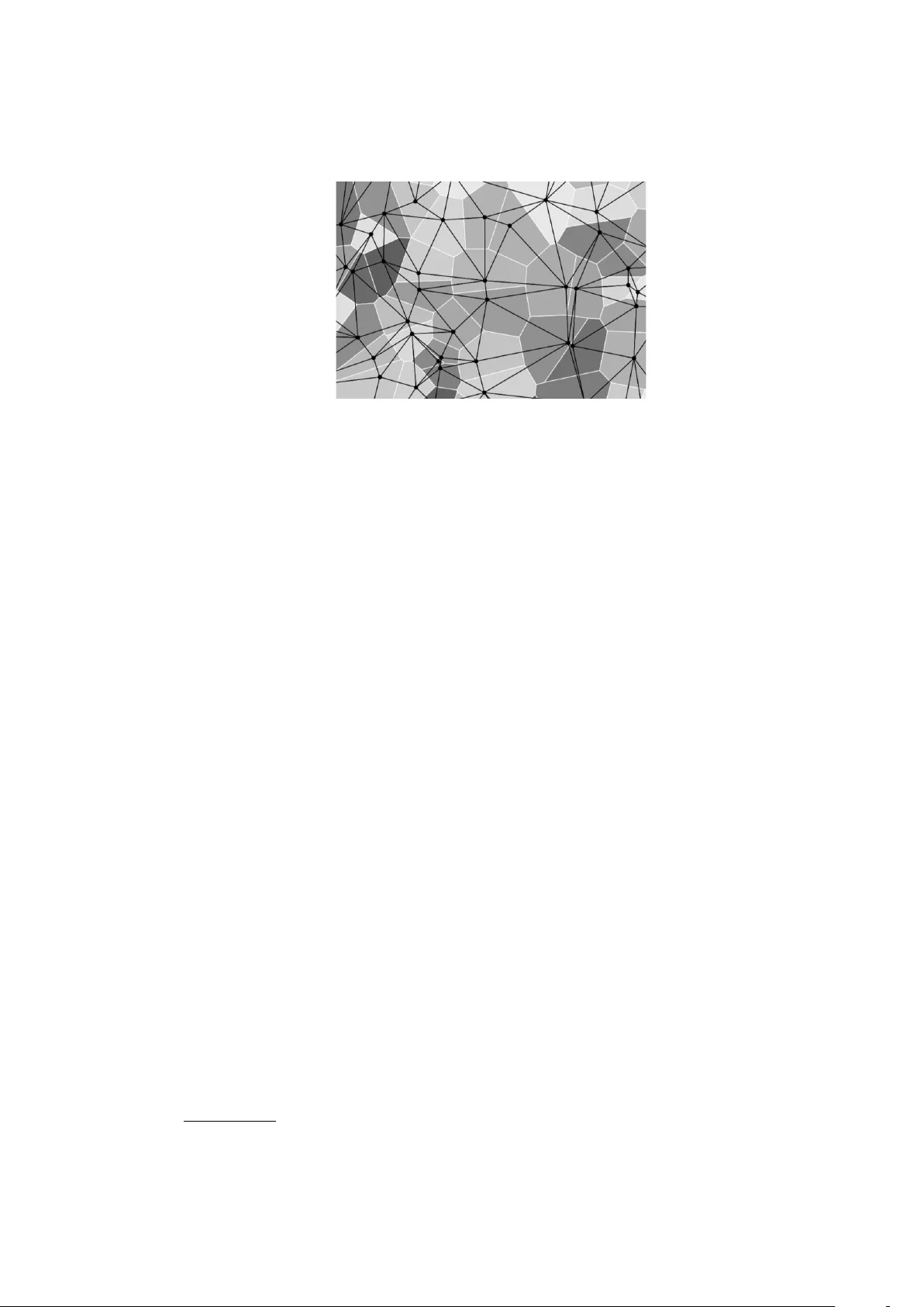
MOMENT BOUNDS AND EX CLUSION PR OCESSES ON RANDOM DELA UNA Y TRIANGULA TIONS WITH CONDUCT ANCES ALESSANDRA F AGGIONA TO AND CRISTINA T A GLIAFERRI Abstra ct. W e consider the V oronoi tessellation asso ciated to a stationary simple point pro cess on R d with ﬁnite and p ositiv e intensit y . W e introduce the Delaunay triangulation as its dual graph, i.e. the graph with vertex set giv en by the p oin t pro cess and with edges b et ween vertices whose V oronoi cells share a ( d − 1) –dimensional face. W e also attach to each edge a random w eight, called conductance. W e pro vide suﬃcient conditions ensuring the in tegrability w.r.t. the P alm distribution of sev eral quantities as w eigh ted degrees and associated moments. These integrabilit y prop erties are crucial in applications, as they allo w to apply existing results on random walks, resistor net w orks and the symmetric simple exclusion pro cesses with random conductances (cf. [1, 11, 12, 13, 14, 15]). F or the latter, while the moment b ounds ensure its w ell deﬁniteness and several properties, the same does not hold when the jump rates are not symmetric, i.e. for a generic simple exclusion pro cess. In this case, by using a criterion from [13], w e recov er construction and prop erties of the simple exclusion pro cess whenever the simple p oin t pro cess has ﬁnite range of dep endence and the conductances are uniformly upp er b ounded. This last result relies on a suitable analysis of Bernoulli b ond p ercolation on the Delauna y triangulation inspired by [2, 3]. All the ab o v e results remain v alid if the simple p oin t pro cess is stationary with resp ect to integer translations. Keywor ds : V oronoi tessellation, Delaunay triangulation, conductance ﬁeld, P alm distribution, momen t bounds, b ond p ercolation on Delaunay triangu- lation. AMS 2010 Subje ct Classiﬁc ation : 60G55, 60K37, 35B27. This p ap er is de dic ate d to Claudio L andim on the o c c asion of his 60th birthday. 1. Intr oduction Random structures generated b y p oin t pro cesses in R d pro vide a natural and v ersatile framew ork for mo deling disordered media and spatially inhomo- geneous systems. Among these, the Delaunay triangulation associated with a simple p oin t pro cess (i.e. a lo cally ﬁnite conﬁguration of p oin ts) plays a partic- ularly imp ortan t role, as it enco des the geometric adjacency relations induced b y the corresp onding V oronoi tessellation. When random w eights (or c onduc- tanc es ) are assigned to the edges of the Delaunay triangulation, one obtains a weigh ted random graph that serves as a fundamen tal mo del for studying sto c hastic processes in random environmen ts. 1 2 A. F AGGIONA TO AND C. T A GLIAFERRI The aim of this pap er is to in v estigate quan titativ e prop erties of suc h w eigh ted Delauna y graphs, with a particular fo cus on momen t b ounds and integrabilit y conditions for k ey functionals of the system. These functionals include, for instance, w eigh ted degrees and sums of conductances around a typical p oin t, as well as higher-order quan tities inv olving spatial displacemen ts. Establish- ing suitable integrabilit y prop erties for some of these ob jects w.r.t. the P alm distribution (as P x : x ∼ 0 | x | ζ , λ 0 , λ 2 ,  deg DT( ξ ) (0)  p , µ ω (0) p , ν ω (0) p in tro duced in Section 4) is a crucial step in the analysis of several probabilistic models on the Delaunay triangulation, including random w alks, electrical resistor net- w orks, and interacting particle systems such as the symmetric simple exclusion pro cess, all among random conductances (cf. [1, 11, 12, 13, 14, 15]). A central diﬃcult y in this setting stems from the interpla y b et w een geomet- ric randomness and probabilistic dep endence. The structure of the Delauna y triangulation is highly sensitiv e to the conﬁguration of points, and ev en lo cal mo diﬁcations of the p oin t pro cess ma y induce long-range c hanges in the graph. This mak es it c hallenging to control quan tities suc h as the degree of a vertex or the spatial range of its neigh b ors. T o o vercome this diﬃculties, inspired by [23, 26] we develop an estimate pro cedure based on the so-called fundamen- tal r e gion . F or previous moment b ounds w e refer to [23, Section 11] (where the assumptions are m uc h stronger than ours) and [26] for the Poisson point pro cess. Our analysis is carried out in the general setting of simple p oin t pro cesses that are stationary and ergodic, with ﬁnite and p ositiv e in tensity . W e consider a broad class of mo dels, ranging from pro cesses with ﬁnite range of dep en- dence to more general situations where correlations may deca y slo wly or are not explicitly controlled. In addition, w e treat p oint pro cesses exhibiting p os- itiv e asso ciation, whic h allo ws us to exploit monotonicit y prop erties in the deriv ation of momen t b ounds. T o give a ﬂav or of applications, in Section 7 w e discuss P oisson p oin t pro cesses, determinantal point processes, and Gibbsian p oin t pro cesses arising in statistical mec hanics. In addition to momen t estimates, w e also in vestigate Bernoulli b ond p er- colation on the Delaunay triangulation. In particular, we pro vide conditions under whic h the resulting random graph has only ﬁnite connected compo- nen ts, a prop erty that is relev an t for the graphical construction of exclusion pro cesses with p ossibly non-symmetric jump rates and for the deriv ation of some fundamental prop erties (cf. [13]). This analysis is restricted to the case of b ounded conductances and simple point pro cesses with ﬁnite-range dep en- dence. T o p erform this analysis we use the “ Z d –pro cess" approac h dev elop ed in [2, 3] for Poisson p oint pro cesses and w e extend it to the case of ﬁnite range of dep endence. Outline of the pap er . In Section 2 we introduce the V oronoi tessellation, the Delauna y triangulation and the conductance ﬁeld and we introduce some fundamen tal assumptions. In Section 3 w e recall the deﬁnition of P alm dis- tribution and some of its properties. In Section 4 w e discuss the fundamental region and present our main results concerning the in tegrability w.r.t. the 3 P alm distribution of P x : x ∼ 0 | x | ζ , λ 0 , λ 2 ,  deg DT( ξ ) (0)  p , µ ω (0) p , ν ω (0) p . This in tegrabilit y is required when applying some existing results on random w alks, resistor net w orks and SSEPs. In Section 5 w e illustrate this application in the case of the SSEP . In Section 6 we give a criterion assuring the construction and several prop erties of the SEP on the Delauna y triangulation with conduc- tances. Sp eciﬁc examples are discussed in Section 7. The remaining sections and the app endix are dev oted to proofs. 2. Model 2.1. Basic notation. W e start b y ﬁxing some basic notation. W e denote b y N the set of non-negative in tegers, while we write R + for [0 , + ∞ ) . The v ectors e 1 , . . . , e d form the canonical basis of R d , L ( A ) is the Leb esgue measure of the Borel set A ⊂ R d , a · b is the scalar pro duct of a, b ∈ R d , | a | and | a | ∞ are resp ectiv ely the Euclidean and the uniform norm of a ∈ R d . Giv en r > 0 and x ∈ R d , the ball B r ( x ) and the b oxes Λ r ( x ) and Λ r are deﬁned as B r ( x ) = { y ∈ R d : | y − x | ≤ r } , Λ r := [ − r , r ] d , Λ r ( x ) := x + Λ r . (1) Giv en a top ological space X , without further mention, X will b e though t of as a measurable space endow ed with the σ –algebra B ( X ) of its Borel subsets. W e denote by 1 A or 1 ( A ) the indicator function of the ev en t A . If E[ · ] is the exp ectation w.r.t. some probabilit y measure, w e use the notation E[ X , A ] for E[ X 1 A ] , where X is a random v ariable and A is an even t. 2.2. Space N of locally ﬁnite subsets of R d . W e denote b y N the set of lo cally ﬁnite subsets of R d and write ξ for a generic element of N . An element of ξ ∈ N is naturally identiﬁed with the simple counting measure P x ∈ ξ δ x , whic h w e again denote b y ξ with a sligh t abuse of notation. In particular, ξ ( A ) and R R d dξ ( x ) f ( x ) corresp ond respectively to ♯ ( ξ ∩ A ) and P x ∈ ξ f ( x ) for all A ⊂ R d and f : R d → R . This identiﬁcation also allo ws one to endow N with the standard metric used for lo cally ﬁnite measures on R d (see [7, Eq. (A2.6.1), App. A2.6]). Its precise deﬁnition will not be used in what follo ws. F or completeness, we recall that the conv ergence ξ n → ξ in N as n → + ∞ is equiv alen t to each of the following t w o prop erties (see [7, Prop osition A2.6.I I]): • ξ n ( A ) → ξ ( A ) as n → + ∞ for all A ∈ B ( R d ) with ξ ( ∂ A ) = 0 ; • ξ n → ξ v aguely as lo cally ﬁnite measures, i.e. R R d dξ n ( x ) f ( x ) → R R d dξ ( x ) f ( x ) as n → + ∞ for all f ∈ C c ( R d ) . It can b e shown that the Borel σ –algebra B ( N ) is generated b y the sets { ξ ( A ) = n } with A ∈ B ( R d ) and n ∈ N (see [7, Prop osition 7.1.I I I and Corollary 7.1.VI]). The group R d acts on the space N b y translations ( τ x ) x ∈ R d , where τ x ξ := ξ − x ξ ∈ N , x ∈ R d . (2) 4 A. F AGGIONA TO AND C. T A GLIAFERRI Figure 1. V oronoi tessellation and Delaunay triangulation asso ciated to the set ξ , whose p oints are giv en b y the black dots ( d = 2 ). Here ξ is regarded as a subset of R d . The choice of the sign is purely con v en- tional. Its adv an tage in the present context is that, given x ∈ ξ , τ x ξ repre- sen ts the new conﬁguration of p oin ts observ ed b y someone located at x , with Cartesian axes obtained by translating the original ones so that the observer’s p osition b ecomes the new origin 1 . Finally , recall that a simple p oint pr o c ess is a measurable map from a prob- abilit y space to the measure space  N , B ( N )  . 2.3. V oronoi tessellations and Delauna y triangulations. Giv en ξ ∈ N and x ∈ ξ , the V oronoi cell with nucleus x is giv en by V or( x | ξ ) = { y ∈ R d : | y − x | ≤ | y − z | ∀ z ∈ ξ } . The V oronoi tessellation asso ciated with ξ is the collection of the V oronoi cells V or( x | ξ ) , x ∈ ξ (see Figure 1). Since it is a coun table in tersection of closed half-spaces, each V oronoi cell is closed and conv ex. Moreov er, if x  = y in ξ , then the cells V or( x | ξ ) and V or( y | ξ ) either share a ( d − 1) -dimensional face or they do not share any ( d − 1) –dimensional region. Deﬁnition 2.1 (Delauna y triangulation DT( ξ ) ) . Given ξ ∈ N we deﬁne the Delauna y triangulation asso ciate d to ξ as the gr aph DT( ξ ) with vertic es the p oints of ξ and e dges given by the p airs { x, y } with x  = y in ξ such that V or( x | ξ ) and V or( y | ξ ) shar e a ( d − 1) –dimensional fac e (se e Figur e 1). W e write E DT ( ξ ) for the e dges of DT( ξ ) . Given x, y ∈ ξ , we write x ∼ y (understanding the dep endenc e on ξ ) whenever { x, y } ∈ E DT ( ξ ) . W e stress that in computational geometry the notion of Delauna y triangu- lation is slightly diﬀerent and can refer to a complex, whose 0-sk eleton and 1-sk eleton corresp ond to the ab ov e DT( ξ ) . See e.g. [17, Section 10.3]. F or us the Delaunay triangulation is just the graph dual to the V oronoi tessella- tion. W e also p oin t out that, although in Figure 1 the edges of the Delauna y 1 By the ab ov e identiﬁcation of ξ with an atomic measure, deﬁnition (2) guarantees that τ x ξ ( A ) = ξ ( A + x ) for all x ∈ R d and A ∈ B ( R d ) . 5 triangulation in R 2 b ound triangles, this is not alwa ys true for d = 2 (take for example ξ = Z 2 ). In general, the Delaunay triangulation in R d is the 1 – sk eleton of a tessellation made b y d -simplices when p oin ts of ξ are in gener al quadr atic p osition (cf. [17, Chapter 10] and [21] for deﬁnitions and results). W e refer to [25] for suﬃcient conditions on simple p oint processes ensuring that a.s. p oints of ξ are in general quadratic p osition (an example is given b y the homogeneous Poisson p oint pro cess). W e recall (cf. [18, Deﬁnition 1.5]) that a p olyhe dr on in R d is deﬁned as the in tersection of ﬁnitely man y closed half-spaces, while a c onvex p olytop e in R d is deﬁned as the conv ex hull of ﬁnitely many p oints in R d . It is known that b ounded p olyhedra coincide with con v ex p olytop es (cf. [18, Theorems 1.20 and 1.22]). As sho wn b elo w, for our simple p oint processes a.s. the V oronoi cells will be conv ex p olytop es. Therefore it is natural to in troduce the follo wing subset N pol ⊂ N : Deﬁnition 2.2 (Set N pol ) . W e denote by N pol the family of ξ ∈ N such that the V or onoi c el l V or( x | ξ ) is a c onvex p olytop e (e quivalently, a b ounde d p olyhe dr on) for al l x ∈ ξ . One can prov e that N pol b elongs to B ( N ) . Note that, according to the abov e deﬁnition, ∅ ∈ N pol . In App endix A.1 w e prov e the following criterion ensuring that ξ ∈ N pol , where the orthant Q σ is deﬁned as follows: Q σ := { x ∈ R d : σ i x i > 0 for 1 ≤ i ≤ d } , σ ∈ {− 1 , +1 } d . Lemma 2.3. If ξ ∈ N satisﬁes ξ ∩ ( x + Q σ )  = ∅ for al l x ∈ Z d and al l σ ∈ {− 1 , +1 } d , then ξ ∈ N pol . 2.4. Delauna y triangulation in a random en vironmen t with a conduc- tance ﬁeld. W e consider a probability space (Ω , F , P ) and denote by E[ · ] the exp ectation w.r.t. P . A generic conﬁguration ω ∈ Ω has to b e thought of as describing the envir onment of the system under inv estigation. W e assume that the additive group R d (endo w ed with the Euclidean metric) acts on the probability space. The action is given b y a family of maps ( θ x ) x ∈ R d with θ x : Ω → Ω such that (P1) θ 0 = 1 , (P2) θ x ◦ θ y = θ x + y for all x, y ∈ R d , (P3) the map R d × Ω ∋ ( x, ω ) 7→ θ x ω ∈ Ω is measurable. Deﬁnition 2.4 (Simple p oint pro cess ω 7→ ˆ ω ) . W e ﬁx a simple p oint pr o c ess Ω ∋ ω → ˆ ω ∈ N deﬁne d on the pr ob ability sp ac e (Ω , F , P ) . In what fol lows we write P for its law on N and we write E [ · ] for the asso ciate d exp e ctation. F or later use we recall some basic terminology . P is called stationary if P ( θ x A ) = P ( A ) for all x ∈ R d and A ∈ F . A set A ⊂ Ω is called tr anslation invariant if θ x A = A for all x ∈ R d . P is called er go dic if P ( A ) ∈ { 0 , 1 } for an y translation in v ariant set A ∈ F . Strictly sp eaking, stationarit y , translation in v ariance and ergo dicit y are w.r.t. the action ( θ x ) x ∈ R d on Ω (but the action will b e understo o d in what follows). The same deﬁnitions hold when replacing 6 A. F AGGIONA TO AND C. T A GLIAFERRI Ω , F , P , θ x b y N , B ( N ) , P , τ x resp ectiv ely (recall (2)). If P is stationary , then the intensity of the SPP (or of P ) is denoted by m : m := E  ˆ ω ([0 , 1] d )  = E  ξ ([0 , 1] d )  . (3) W e recall the so-called zer o/inﬁnity pr op erty for stationary SPP (cf. [7, Prop o- sition 10.1.IV]): P stationary = ⇒ P ( ξ = ∅ or ♯ξ = ∞ ) = 1 . (4) As pro v ed in App endix A.2, an imp ortant consequence of the stationarity of P is the following: Lemma 2.5. If P is stationary, then P ( N pol ) = 1 . W e now introduce the last ingredient of our mo del: Deﬁnition 2.6 (Conductance ﬁeld) . W e assume to have a me asur able map (c al le d conductance ﬁeld ) Ω × R d × R d ∋ ( ω , x, y ) 7→ c x,y ( ω ) ∈ [0 , + ∞ ) such that c x,y ( ω ) = c y ,x ( ω ) . As will b e made clear from our applications, c x,y ( ω ) will b e relev ant only for x ∼ y in DT( ˆ ω ) . Moreo v er, without loss of generalit y and to simplify some form ulas b elow, we conv ey that c x,x ( ω ) = 0 and c x,y ( ω ) = 0 if { x, y } is not an edge of DT( ˆ ω ) . F or sev eral results we will take the follo wing assumptions (they will b e stated explicitly): Main Assumptions : The fol lowing holds: (A1) The pr ob ability me asur e P is stationary and P ( { ω ∈ Ω : ˆ ω = ∅} ) = 0 . (A2) The simple p oint pr o c ess Ω ∋ ω 7→ ˆ ω ∈ N has ﬁnite and p ositive intensity m ( cf. Eq. (3)) . (A3) F or some tr anslation invariant me asur able set Ω ∗ ⊂ Ω with P (Ω ∗ ) = 1 the fol lowing c ovariant r elations ar e satisﬁe d for al l ω ∈ Ω ∗ : d θ x ω = τ x ˆ ω ∀ x ∈ R d , (5) c y − x,z − x ( θ x ω ) = c y ,z ( ω ) ∀ x ∈ R d , ∀ y ∼ z ∈ DT( ˆ ω ) . (6) Supp ose for the momen t just that P is stationary and (5) holds for all ω ∈ Ω ∗ as in (A3). Then, by Lemma A.1–(i), also P is stationary . Moreov er, the ev en t A := { ω ∈ Ω ∗ : ˆ ω = ∅} is translation in v ariant. Hence, excluding the trivial case P ( A ) = 1 , at cost to decomp ose P and condition on A c , w e can alw a ys reduce to the case P ( { ω ∈ Ω : ˆ ω = ∅} ) = 0 as in (A1). When ˆ ω = ∅ the Delauna y triangulation and all our statements b ecome trivial, hence the request P ( { ω ∈ Ω : ˆ ω = ∅} ) = 0 in (A1) combined with (A3) is just to a v oid trivialities, it is without loss of generality and could be remov ed as w ell. W e also p oint out that the ab ov e request implies that the in tensity m of the SPP 7 is not zero, but we hav e stated this explicitly in (A2) since it is relev an t in the rest. Under the abov e Main Assumptions, the exp ected num ber of p oints of the SPP in a generic set B ∈ B ( R d ) equals m L ( B ) , where L ( B ) denotes the Leb esgue measure of B . Moreov er, see (4) and Lemma 2.5, it holds P  { ω ∈ Ω : ♯ ˆ ω = + ∞} ) = 1 and P  { ω ∈ Ω : ˆ ω ∈ N pol }  = P ( N pol ) = 1 . T o give a more graphical in terpretation of (A3), let us assign to ω the fol- lo wing weigh ted graph G ( ω ) : Deﬁnition 2.7 (Graph G ( ω ) ) . Given ω ∈ Ω , the weighte d undir e cte d gr aph G ( ω ) is deﬁne d as the Delaunay triangulation on ˆ ω , wher e e ach e dge { x, y } is assigne d the weight e qual to its c onductanc e c x,y ( ω ) . Then the co v arian t relations (5) and (6) in Assumption (A3), together, are equiv alent to the identit y of w eigh ted graphs G ( θ x ω ) = G ( ω ) − x ∀ x ∈ R d , where G ( ω ) − x is the weigh ted graph obtained b y translating G ( ω ) in R d along the v ector − x (in the translation, each edge keeps its o wn weigh t). Remark 2.8. W e have c onsider e d the actions of the gr oup G := R d on the pr ob ability sp ac e Ω by ( θ g ) g ∈ G and on the sp ac e N by ( τ g ) g ∈ G . As in [11, 12, 14] one c an extend the analysis by c onsidering also the action of the gr oup G := Z d . In b oth c ases G = R d and G = Z d one c an also de al with τ g of the form τ g ξ := ξ − V g , wher e V is a ﬁxe d d × d invertible matrix. These extensions ar e natur al for example when de aling with simple p oint pr o c esses on crystal lattic es (cf. [11, Section 5.2] , [12, Section 5.6] ). A l l the r esults pr esente d b elow c an b e r estate d in this extende d setting with slight mo diﬁc ations in the pr o ofs. 3. P alm distributions P 0 and P 0 In this section, we assume (A1), (A2) and (A3). Deﬁnition 3.1 (Palm distribution P 0 ) . The Palm distribution P 0 , asso ciate d to P and the simple p oint pr o c ess ω 7→ ˆ ω , is the pr ob ability me asur e on Ω c onc entr ate d on Ω 0 := { ω ∈ Ω : 0 ∈ ˆ ω } such that P 0 ( A ) = 1 m Z Ω d P ( ω ) Z [0 , 1] d d ˆ ω ( x ) 1 A ( θ x ω ) ∀ A ∈ F . (7) The exp e ctation asso ciate d to P 0 is denote d by E 0 . W e recall that ˆ ω is naturally iden tiﬁed with the atomic measure P x ∈ ˆ ω δ x , hence R [0 , 1] d d ˆ ω ( x ) f ( x ) has to b e though t of as P x ∈ ˆ ω ∩ [0 , 1] d f ( x ) . W e refer the in terested reader to [7, Chapter 12], [12, Section 2 and App endix B] and references therein for more details on the P alm distribution P 0 . Roughly , P 0 := P ( ·| Ω 0 ) . Since by stationarity of P it can b e prov ed that P (Ω 0 ) = 0 , the ab ov e iden tit y is meaningless but it can b e rigorously formalized by means of regular conditional probabilities as in [7, Chapter 12]. 8 A. F AGGIONA TO AND C. T A GLIAFERRI Since b y Lemma A.1 the law P on N of our simple p oint pro cess is sta- tionary w.r.t. the action ( τ x ) x ∈ R d on N and has ﬁnite p ositiv e intensit y m = E [ ξ ([0 , 1] d )] , also the P alm distribution P 0 asso ciated to P is well deﬁned (cf. [7, Chapter 12]). W e recall that P 0 is the probabilit y measure on N concen trated on N 0 := { ξ ∈ N : 0 ∈ ξ } such that P 0 ( A ) = 1 m Z N d P ( ξ ) Z [0 , 1] d dξ ( x ) 1 A ( τ x ξ ) ∀ A ∈ B ( N ) . (8) Giv en A ∈ B ( N ) and setting B := { ω ∈ Ω : ˆ ω ∈ A } , for all ω ∈ Ω ∗ w e hav e 1 A ( τ x ˆ ω ) = 1 B ( θ x ω ) since d θ x ω = τ x ˆ ω b y (5). Therefore, b y comparing (7) with (8), w e get P 0 ( A ) = P 0 ( B ) , i.e. P 0 ( A ) = P 0 ( ˆ ω ∈ A ) ∀ A ∈ B ( N ) . In what follo ws, w e will use a generalization of (8) called Campb ell’s formula (cf. [7, Eq. (12.2.4), Theorem 12.2.I I]): for each measurable function f : R d × N 0 → [0 , + ∞ ) it holds Z N 0 d P 0 ( ξ ) Z R d dxf ( x, ξ ) = 1 m Z N d P ( ξ ) Z R d dξ ( x ) f ( x, τ x ξ ) . (9) F or completeness, although not used b elo w, w e recall that a similar form ula holds for P (see [12, App endix B]). 4. Main resul ts: moment bounds w.r.t. P 0 In this section, we make Assumptions (A1), (A2) and (A3). W e recall that the P alm distribution P 0 has support in Ω 0 := { ω ∈ Ω : 0 ∈ ˆ ω } and that E 0 [ · ] denotes the asso ciated exp ectation (cf. Deﬁnition 3.1). Moreo v er, E[ · ] denotes the expectation w.r.t. P , while E [ · ] denotes the expectation w.r.t. P (the latter is the image of P b y the map ω 7→ ˆ ω ). F or k = 0 , 2 we deﬁne the functions λ k : Ω 0 → [0 , + ∞ ] as λ k ( ω ) := Z R d d ˆ ω ( x ) c 0 ,x ( ω ) | x | k = X x : x ∼ 0 c 0 ,x ( ω ) | x | k . (10) A fundamental condition in order to apply the results in [11, 12, 14] is that λ 0 , λ 2 ∈ L 1 ( P 0 ) . In this section w e will pro vide suﬃcient conditions for the ab o ve in tegrability as w ell as for the integrabilit y of P x : x ∼ 0 | x | ζ for ζ ≥ 0 (as in termediate step). As in [1], given ω ∈ Ω 0 , w e deﬁne 2 µ ω (0) := λ 0 ( ω ) = X x : x ∼ 0 c 0 ,x ( ω ) and ν ω (0) := X x : x ∼ 0 1 c 0 ,x ( ω ) . Sev eral results in [1] require that µ ω (0) ∈ L p ( P 0 ) and ν ω (0) ∈ L p ′ ( P 0 ) for p, p ′ ∈ [1 , + ∞ ] satisfying a suitable inequalit y . In this section w e will pro vide 2 Although µ ω (0) = λ 0 ( ω ) , we prefer to introduce also the notation µ ω (0) since closer to the one used in the moment b ound conditions app earing in several pap ers ab out the random conductance mo del on Z d or subgraphs. 9 suﬃcien t conditions assuring in general the momen t bound µ ω (0) ∈ L p ( P 0 ) , or ν ω (0) ∈ L p ( P 0 ) , for p ∈ [1 , + ∞ ) . As an in termediate step, w e will also in v estigate the integrabilit y of  deg DT( ˆ ω ) (0)  p . When pro viding suﬃcient conditions for λ 0 , λ 2 ∈ L 1 ( P 0 ) , µ ω (0) ∈ L p ( P 0 ) or ν ω (0) ∈ L p ( P 0 ) , w e will treat t w o extreme situations concerning the deca y of correlation of the SPP ω 7→ ˆ ω : one in whic h the SPP has a ﬁnite range of dep endence, and a generic case in whic h no information on the decay of correlations is a v ailable. W e p oin t out that the metho ds used in the pro ofs could b e further optimized for situations exhibiting an intermediate form of correlation decay . In addition to the ab o v e extreme t wo cases, we also treat the case in whic h the SPP has p ositive asso ciation. T o state our results, given γ > 0 , we deﬁne ρ γ := E  ˆ ω ([0 , 1] d ) γ  = E  ξ ([0 , 1] d ) γ  . (11) W e note that, by assumption (A2), ρ 1 = m ∈ (0 , + ∞ ) . 4.1. F undamen tal region. Before presen ting our results w e discuss the so– called fundamen tal region D( x | ξ ) asso ciated to a vertex x ∈ ξ of a Delauna y triangulation. This concept is crucial for the deriv ation of the momen t b ounds presen ted b elow. Deﬁnition 4.1 (F undamental region) . Given ξ ∈ N pol and x ∈ ξ , the funda- men tal region D( x | ξ ) of x is given by the union of the close d b al ls c enter e d at v and of r adius | v − x | , wher e v varies among the vertic es of the c el l V or( x | ξ ) (se e Figur e 2–(left)). Since under our main assumptions (A1), (A2), and (A3) we hav e P ( N pol ) = 1 , we ma y , without loss of generalit y , restrict our attention to ξ ∈ N pol . W e therefore do not attempt to formulate the results b elo w under weak er geometric assumptions on ξ . F or example, if ξ ∈ N pol consists of tw o points, then the V oronoi cells of ξ are t w o half-spaces and therefore hav e no v ertices. On the other hand, there is no need for our purp oses to consider suc h degenerate situations. As stated in Lemma 9.1 in Section 9, given ξ ∈ N pol and x ∈ ξ , all v ertices adjacen t to x in DT( ξ ) b elong to D ( x | ξ ) . W e set (see Figure 2–(right)) I := { z ∈ Z d : | z | ∞ = d } (12) and, giv en z ∈ R d and ℓ > 0 , K ℓ ( z ) := z ℓ +  − ℓ/ 2 , ℓ/ 2  d = Λ ℓ/ 2 ( z ℓ ) . (13) Then, in Section 9 (cf. Lemma 9.1 and Lemma 9.3) we will pro v e the following c hain of implications, where deg DT( ξ ) ( x ) denotes the degree of x in the graph 10 A. F AGGIONA TO AND C. T A GLIAFERRI Figure 2. (Left) Blac k dots are points of ξ . V or( x | ξ ) is the grey region. D ( x | ξ ) is the union of the balls. (Right) In grey , the shield of b oxes K ℓ ( z ) with z ∈ I . DT( ξ ) : ξ ∈ N pol ∩ N 0 and ξ  K ℓ ( z )  > 0 for all z ∈ I = ⇒ { y : y ∼ 0 } ⊂ D (0 | ξ ) ⊂ B 6 ℓd 2 (0) = ⇒ ( deg DT( ξ ) (0) ≤ ξ  B 6 ℓd 2 (0)  max {| y | : y ∼ 0 } ≤ 6 ℓd 2 . (14) The ab o ve implications will be the starting point for the deriv ation of the momen t b ounds presented b elo w. 4.2. In tegrabilit y of P x : x ∼ 0 | x | ζ , λ 0 , λ 2 w.r.t. P 0 . T o state our results, w e ﬁrst recall tw o deﬁnitions concerning SPPs. Deﬁnition 4.2 (SPP with ﬁnite range of dep endence) . A pr ob ability me asur e P on N has ﬁnite range of dep endence if ther e exists L > 0 such that, for any Bor el sets A, B ⊂ R d having Euclide an distanc e at le ast L , the r andom variables ξ ∩ A and ξ ∩ B deﬁne d on the pr ob ability sp ac e ( N , B ( N ) , P) ar e indep endent. In this c ase, we say that the r ange of dep endenc e is smal ler than L . Deﬁnition 4.3 (SPP with negativ e/p ositiv e asso ciation) . A pr ob ability me a- sur e P on N has p ositiv e association if for any n, k ≥ 0 , any we akly incr e asing functions f : R n + → R and g : R k + → R and any family of p airwise disjoint b ounde d Bor el sets A 1 , A 2 , . . . , A n , B 1 , B 2 , . . . , B k in R d , it holds Co v  f  ξ ( A 1 ) , ξ ( A 2 ) , . . . , ξ ( A n )  , g  ξ ( B 1 ) , ξ ( B 2 ) , . . . , ξ ( B k )   ≥ 0 , (15) whenever the two r andom variables app e aring in the ab ove c ovarianc e has ﬁnite se c ond moment w.r.t. P . The pr ob ability me asur e P is said to have negativ e asso ciation if the same holds with ≤ inste ad of ≥ in (15) . 11 Remark 4.4. E h Q n i =1 f i ( ξ ( A i )) i ≤ Q n i =1 E h f i ( ξ ( A i )) i whenever P has ne g- ative asso ciation, A 1 , . . . , A n ar e p airwise disjoint b ounde d Bor el sets in R d and f 1 , . . . , f n : R + → R + ar e b ounde d functions al l we akly incr e asing or al l we akly de cr e asing. T ake for example n = 3 and f i de cr e asing. Then E [ f 1 f 2 f 3 ] = E [( − f 1 f 2 )( − f 3 )] ≤ E [ − f 1 f 2 ] E [ − f 3 ] = E [ f 1 f 2 ] E [ f 3 ] by (15) , sinc e − f 1 f 2 and − f 3 ar e we akly incr e asing (a further iter ation al lows to c onclude). W e no w in tro duce a condition concerning the so–called void pr ob abilities relev ant for our results. T o this aim, recall the deﬁnition of B r ( x ) , Λ r and Λ r ( x ) giv en in (1). Deﬁnition 4.5 (Condition C ( α ) ) . Given α > 0 we say that Condition C ( α ) is satisﬁe d if ther e exists κ > 0 such that P ( ξ (Λ ℓ ) = 0) ≤ κ ℓ − α ∀ ℓ ≥ 1 , (16) The follo wing tw o propositions can b e readily prov ed. F or completeness we giv e their pro ofs in App endixes A.3 and A.4. Prop osition 4.6. If P has ﬁnite r ange of dep endenc e or it has ne gative asso- ciation, then for a suitable c onstant c > 0 we have P ( ξ (Λ ℓ ) = 0) ≤ e − cℓ d for al l ℓ ≥ 1 . In p articular, P satisﬁes Condition C ( α ) for any α > 0 . W e generalize the ab ov e result in the next prop osition. Giv en U ⊂ R d w e denote b y F U the σ –algebra of even ts determined b y the behavior of ξ on U . W e set T a := F Λ c a . Prop osition 4.7. Supp ose that lim k → + ∞ ∥ P ( ξ (Λ 1 / 2 ) = 0 |T k ) − P ( ξ (Λ 1 / 2 ) = 0) ∥ ∞ = 0 . (17) Then for a suitable c onstant c > 0 we have P ( ξ (Λ ℓ ) = 0) ≤ e − cℓ d for al l ℓ ≥ 1 . In p articular, P satisﬁes Condition C ( α ) for any α > 0 . W e can ﬁnally state our main results. Theorem 4.8. Assume (A1), (A2) and (A3). Then, given ζ ≥ 0 , it holds E 0  P x ∼ 0 | x | ζ  < + ∞ if at le ast one of the fol lowing hyp otheses is satisﬁe d: (H1) ρ γ < + ∞ for some γ > 2 and Condition C ( α ) holds for some α with α > γ γ − 2 ( d + ζ ) ; (18) (H2) ρ 2 < + ∞ and P has ﬁnite r ange of dep endenc e; (H3) ρ 2 < + ∞ , P has p ositive asso ciation and Condition C ( α ) holds for some α > d + ζ . Pr o of. The claim is an immediate consequence of Prop osition 10.2 and Corol- lary 10.4. □ Theorem 4.9. In addition to (A1), (A2), (A3), we supp ose that ther e exists a lo c al ly b ounde d me asur able function ϕ : R + → R + and c onstants C 0 > 0 and ζ ≥ 0 such that 12 A. F AGGIONA TO AND C. T A GLIAFERRI • ϕ ( r ) ≤ C 0 r − 2+ ζ for r ≥ 1 ; • for P 0 –a.a. ω it holds E 0  c 0 ,x ( ω ) | ˆ ω  ≤ ϕ ( | x | ) ∀ x : x ∼ 0 . (19) Then λ 0 , λ 2 ∈ L 1 ( P 0 ) if at le ast one hyp othesis b etwe en (H1), (H2) and (H3) in The or em 4.8 is satisﬁe d. Theorem 4.9 will b e prov ed in Section 12. By taking ϕ constant and ζ = 2 in the ab ov e theorem, w e immediately get the following result whic h co v ers in particular the relev an t case of unit conductances b etw een nearest-neighbor v ertices, as w ell as the case of conductances that are i.i.d. conditionally on P ( ·| ˆ ω ) with distribution having ﬁnite mean (see Prop osition 4.12 b elow): Corollary 4.10. In addition to (A1), (A2), (A3), we supp ose that for some C ∗ > 0 and for P 0 –a.a. ω it holds E 0  c 0 ,x ( ω ) | ˆ ω  ≤ C ∗ ∀ x : x ∼ 0 . (20) Then λ 0 , λ 2 ∈ L 1 ( P 0 ) if at le ast one of the fol lowing hyp otheses is satisﬁe d: (H1’) ρ γ < + ∞ for some γ > 2 and Condition C ( α ) holds for some α > γ γ − 2 ( d + 2) ; (H2’) ρ 2 < + ∞ and P has ﬁnite r ange of dep endenc e; (H3’) ρ 2 < + ∞ , P has p ositive asso ciation and Condition C ( α ) holds for some α > d + 2 . If ϕ decays suﬃciently fast, then Theorem 4.9 and its pro of are not optimal and one can give a muc h simpler pro of of the in tegrabilit y of λ 0 , λ 2 : Prop osition 4.11. In addition to (A1), (A2), (A3), we supp ose that ther e exists a lo c al ly b ounde d me asur able function ϕ : R + → R + and c onstants C 0 , ε > 0 such that • ϕ ( r ) ≤ C 0 r − d − 2 − ε for r ≥ 1 ; • for P 0 –a.a. ω it holds E 0  c 0 ,x ( ω ) | ˆ ω  ≤ ϕ ( | x | ) for al l x : x ∼ 0 . Then, if ρ 2 < + ∞ , we have λ 0 , λ 2 ∈ L 1 ( P 0 ) . Prop osition 4.11 will b e prov ed in Section 12. In the next Prop osition w e giv e a suﬃcient condition ensuring (20) in a relev ant application. F or later use, w e form ulate the result in a more general form. F or (20) it is enough to tak e φ ( t ) := t . Prop osition 4.12. L et φ : R + → R b e a me asur able function. Supp ose that under P ( ·| ˆ ω ) the c onductanc es c x,y ( ω ) with { x, y } ∈ E DT ( ˆ ω ) ar e indep endent r andom variables with distribution ν | x − y | p ar ameterize d by the distanc e | x − y | and such that sup r> 0 R ∞ 0 dν r ( t ) φ ( t ) ≤ C ∗ . Then for P 0 –a.a. ω it holds E 0  φ  c 0 ,x ( ω )  | ˆ ω  ≤ C ∗ ∀ x : x ∼ 0 . (21) Pr o of. Let P b e the la w of the SPP . Without loss, we can tak e as space Ω the set { ( ξ , Θ) : ξ ∈ N pol , Θ ∈ (0 , + ∞ ) E DT ( ξ ) } . W e set ˆ ω := ξ and c x,y ( ω ) := Θ { x,y } if ω = ( ξ , Θ) . Finally we supp ose that the probability measure P on Ω 13 corresp onds to sampling ξ with law P , and afterwards assigning indep endently a conductance to the edge { x, y } ∈ E DT ( ξ ) with distribution ν | x − y | . Then, by using Campb ell’s formula, one can easily deriv e that the Palm distribution P 0 corresp onds to sampling ξ with the P alm distribution P 0 asso ciated to P , and afterw ards assigning indep enden tly a conductance to the edge { x, y } ∈ E DT ( ξ ) with distribution ν | x − y | . It then follo ws that max x : x ∼ 0 E 0  φ  c 0 ,x ( ω )  | ˆ ω  ≤ sup r> 0 R ∞ 0 dν r ( t ) φ ( t ) ≤ C ∗ . □ 4.3. In tegrabilit y of  deg DT( ˆ ω ) (0)  p , µ ω (0) p and ν ω (0) p w.r.t. P 0 . Fixed p ∈ [1 , + ∞ ) , b elow we will pro vide conditions ensuring that E 0  deg DT( ˆ ω ) (0) p  < + ∞ . Let us now sho w ho w this momen t b ound is related to the integrabilit y of µ ω (0) p and ν ω (0) p w.r.t. P 0 . Let p ∗ b e the exp onen t conjugate to p (i.e. p − 1 + p − 1 ∗ = 1 ). By Hölder’s inequalit y , w e ha v e µ ω (0) = X x : x ∼ 0 c 0 ,x ( ω ) ≤  X x : x ∼ 0 c 0 ,x ( ω ) p  1 p  deg DT( ˆ ω ) (0)  1 p ∗ . Hence w e hav e (also by conditioning w.r.t. ˆ ω ) E 0  µ ω (0) p  ≤ E 0 h X x : x ∼ 0 c 0 ,x ( ω ) p  deg DT( ˆ ω ) (0) p p ∗ i ≤ E 0 h X x : x ∼ 0 E 0 [ c 0 ,x ( ω ) p | ˆ ω ]  deg DT( ˆ ω ) (0) p p ∗ i . (22) Supp ose no w that for some constan t C < + ∞ it holds that, for P 0 –a.a. ω , sup x : x ∼ 0 E 0 [ c 0 ,x ( ω ) p | ˆ ω ] ≤ C . Then, using that 1 + p/p ∗ = p , we get E 0 [ µ ω (0) p ] ≤ C E 0  deg DT( ˆ ω ) (0) p  . Similarly w e get that sup x : x ∼ 0 E 0  1 /c 0 ,x ( ω ) p   ˆ ω  ≤ C implies that E 0 [ ν ω (0) p ] ≤ C E 0  deg DT( ˆ ω ) (0) p  . Note that in this case it must b e c 0 ,x ( ω ) > 0 for all x ∼ 0 . It remains to ensure that E 0  deg DT( ˆ ω ) (0) p  = E 0  deg DT( ξ ) (0) p  < + ∞ . This task is carried out in Section 11. Our ﬁnal result is the following: Theorem 4.13. Fix p ∈ [1 , ∞ ) . In addition to our main assumptions (A1), (A2), (A3), we assume that at le ast one of the fol lowing c ases holds: (C1) ρ γ < + ∞ for some γ > p + 1 and Condition C ( α ) holds for some α > dpγ γ − 1 − p ; (C2) ρ 1+ p < + ∞ and P has ﬁnite r ange of dep endenc e; (C3) ρ 1+ p < + ∞ , P has p ositive asso ciation and Condition C ( α ) holds for some α > dp . Then E 0  deg DT( ˆ ω ) (0) p  < + ∞ and the fol lowing implic ations hold: (a) If P 0 –a.s. sup x : x ∼ 0 E 0  c 0 ,x ( ω ) p | ˆ ω  ≤ C for some C ∈ [0 , ∞ ) , then E 0 [ µ ω (0) p ] < + ∞ . (b) If P 0 –a.s. sup x : x ∼ 0 E 0 h 1 c 0 ,x ( ω ) p | ˆ ω i ≤ C for some C ∈ [0 , ∞ ) , then E 0 [ ν ω (0) p ] < + ∞ . 14 A. F AGGIONA TO AND C. T A GLIAFERRI Pr o of. Due to the discussion b efore the theorem, it is enough to prov e that E 0  deg DT( ˆ ω ) (0) p  < + ∞ . This b ound is an immediate consequence of Propo- sition 11.1 and Corollary 11.2. □ Note that a suﬃcien t condition implying the v alidit y of the the hypotheses in the ab ov e implications (a) and (b) is provided by Prop osition 4.12 with φ ( t ) := t p and φ ( t ) := t − p , resp ectively . 4.3.1. Extensions. Also for E 0 [ µ ω (0) p ] and E 0 [ ν ω (0) p ] one could pro vide re- sults similar to Theorem 4.9 and Prop osition 4.11 b y using the tec hniques dev elop ed in Sections 10 and 11. W e giv e some comments for the inter- ested reader assuming that, for a measurable function ϕ , for P –a.a. ω it holds E 0  c 0 ,x ( ω ) p | ˆ ω  ≤ ϕ ( | x | ) for all x with x ∼ 0 . F rom (22) w e get E 0  µ ω (0) p  ≤ E 0 h X x : x ∼ 0 ϕ ( | x | )  deg DT( ˆ ω ) (0)  p p ∗ i . (23) Deﬁne G ( t ) := sup | x |≤ t ϕ ( | x | ) . Then b y the implication (49) discussed in Sec- tion 10 and using the notation of Section 10, from (23) we get E 0  µ ω (0) p  ≤ ∞ X n =0 G (6 d 2 β n ) E 0 [ ξ (Γ n ) p , T n i . (24) Ab o ve w e ha v e used that ξ (Γ n ) 1+ p p ∗ = ξ (Γ n ) p . Then one could pro ceed as in Section 11 (compare (24) with (67)) to b ound the series in the r.h.s. of (24), obtaining a result in the same spirit of Theorem 4.9. This metho d w orks w ell when ϕ in not decreasing. If ϕ ( r ) is lo cally b ounded and decreases fast, the ab ov e metho d is not the most eﬃcient. In this case one could ﬁx t > 1 and by Hölder’s inequalit y b ound the r.h.s. of (23) by E 0 h X x : x ∼ 0 ϕ ( | x | )  t i 1 t E 0 h deg DT( ˆ ω ) (0)  pt ∗ p ∗ i 1 t ∗ . (25) Ab o ve t ∗ is the exp onen t conjugate to t . T o get that the second factor in the r.h.s. of (25) is ﬁnite, one could use the ﬁrst part of Theorem 4.13, while to b ound the ﬁrst factor in the r.h.s. of (25) one could pro ceed as in the pro of of Prop osition 4.11. Supp ose for example that, for some γ > d , ϕ ( r ) ≤ C 0 r − γ for r ≥ 1 and ϕ is bounded on (0 , 1] . By taking t = 2 and b y applying the Cauc h y–Sc hw arz inequalit y , we hav e E 0 h X x : x ∼ 0 ϕ ( | x | )  t i ≤ X z ∈ Z d : | z | ∞ ≥ 1 X z ′ ∈ Z d : | z ′ | ∞ ≥ 1 | z | − γ ∞ | z ′ | − γ ∞ E 0  ξ (Λ 1 ( z )) ξ (Λ 1 ( z ′ ))  ≤  sup v ∈ Z d : | v | ∞ ≥ 1 E 0  ξ (Λ 1 ( v )) 2   X z ∈ Z d : | z | ∞ ≥ 1 | z | − γ ∞  2 . (26) 15 The ab ov e supremum is ﬁnite when ρ 3 < + ∞ due to Lemma 8.2, while the righ tmost series is ﬁnite as γ > d . The same considerations presen ted abov e for E 0  µ ω (0) p  hold for E 0  ν ω (0) p  when E 0  1 /c 0 ,x ( ω ) p | ˆ ω  ≤ ϕ ( | x | ) for all x with x ∼ 0 . 5. Intermezzo: An applica tion of the integrability of λ 0 , λ 2 ∈ L 1 ( P 0 ) to the SSEP As already men tioned the integrabilit y of λ 0 , λ 2 w.r.t. P 0 is relev ant e.g. in order to apply to Delauna y triangulations the results presented in [11, 12, 13, 14, 15] for random w alks, resistor net w orks and symmetric simple exclusion pro cesses (brieﬂy , SSEPs), all with random conductances. Applications of the in tegrabilit y of µ ω (0) p and ν ω (0) p w.r.t. P 0 can b e found in [1]. In this section w e just provide a brief ov erview of the results in [11, 15] for the SSEP . In the next section we will fo cus on general (also non-symmetric) SEPs. In this se ction we assume the fol lowing 3 : • (A1’) The pr ob ability me asur e P is stationary and er go dic; • (A2); • (A3); • λ 0 , λ 2 ∈ L 1 ( P 0 ) ; • L 2 ( P 0 ) is sep ar able; • c x,y ( ω ) > 0 for al l { x, y } ∈ E DT ( ˆ ω ) for al l ω ∈ Ω ∗ , with Ω ∗ given by (A3). It is easly to chec k that (A1’), (A2) and (A3) imply (A1), (A2) and (A3). Indeed, b y ergo dicit y , the translation inv arian t set { ω ∈ Ω ∗ : ˆ ω = ∅} has P –probability equal to either zero or one. In the latter case, we would ha v e m = 0 , con tradicting (A3). Using also that P (Ω ∗ ) = 1 , w e conclude that P ( ω ∈ Ω : ˆ ω = ∅ ) = 0 . W e point out that the ab o ve assumptions imply the ones in [12] with ex- ception of [12, (A3) and (A9)]. They also imply all the assumptions in [15, Section 3]. In the latter, we discuss ho w the results presented in [11, 12, 14] can b e derived under weak er assumptions than the original ones. As discussed in [12], the separabilit y of L 2 ( P 0 ) is a v ery w eak assumption. A v ery general condition assuring the separability is pro vided in [12] b efore Remark 2.1 there. Deﬁnition 5.1. W e deﬁne the eﬀe ctive homo genize d matrix D as the d × d nonne gative symmetric matrix such that, for al l a ∈ R d , a · D a = inf f ∈ L ∞ ( P 0 ) 1 2 Z Ω 0 d P 0 ( ω ) Z R d d ˆ ω ( x ) c 0 ,x ( ω ) ( a · x − ∇ f ( ω , x )) 2 , (27) wher e ∇ f ( ω , x ) := f ( θ x ω ) − f ( ω ) . 3 The last assumption could indeed b e weak ened: it is suﬃcient that, P –a.s., the graph ob- tained from DT( ˆ ω ) by remo ving the edges { x, y } with zero conductance c x,y ( ω ) is connected. 16 A. F AGGIONA TO AND C. T A GLIAFERRI The ab ov e deﬁnition is well p osed as discussed in [15]. W e consider the SSEP on DT( ˆ ω ) with formal generator L ω f ( η ) = X { x,y }∈E DT( ˆ ω ) c x,y ( ω ) ( f ( η x,y ) − f ( η )) , where η ∈ { 0 , 1 } ˆ ω is the particle conﬁguration, η ( x ) is the particle o ccupation n um b er at x and the conﬁguration η x,y is obtained from η by exchanging the o ccupation num b ers η ( x ) , η ( y ) . As discussed in [15], even for a larger class of w eigh ted graphs G ( ω ) , thanks to the results obtained in [13], under our assumptions and for P –a.a. ω the ab o ve SSEP admits a rigorous graphical construction. It is a F eller process with state space { 0 , 1 } ˆ ω , and the lo cal functions form a core for the generator. Moreo v er [11, Theorem 1] can b e applied, even though not all the assumptions stated there are required in the present setting ([15] indeed ﬁlls this gap). As a consequence, for P –a.a. ω , under diﬀusive space-time rescaling, the ab ov e SSEP on DT( ˆ ω ) satisﬁes a hydrodynamic limit b oth in path space and at ﬁxed times with hydrodynamic equation ∂ t ρ = div  D ∇ ρ  , where ρ ( x, t ) denotes the macroscopic density proﬁle. F or results concerning the equilibrium ﬂuctuations of the abov e SSEP w e refer to [6]. 6. Main resul ts: v alidity of Assumption SEP of [13] In this section w e remov e our main Assumptions (A1), (A2), (A3) and we start from scratch. W e assume, without further mention, the following: (A) On the pr ob ability sp ac e (Ω , F , P ) we have a simple p oint pr o c ess Ω ∋ ω 7→ ˆ ω ∈ N on R d whose law P is stationary (henc e P ( N pol ) = 1 ) and has ﬁnite intensity m := E [ ξ ([0 , 1] d )] . Mor e over for e ach x, y ∈ DT( ˆ ω ) with x ∼ y we assume to have non-ne gative values c o x,y ( ω ) and c o y ,x ( ω ) . W e denote b y E o DT ( ˆ ω ) the family of the edges of DT( ˆ ω ) endo w ed with the orien tation: E o DT ( ˆ ω ) := { ( x, y ) , ( y , x ) : { x, y } ∈ E DT ( ˆ ω ) } . While the well-deﬁnedness of the SSEP of DT( ˆ ω ) is equiv alent to the w ell- deﬁnedness of the random w alk ( X ω t ) t ≥ 0 as deriv ed in [13, Section 3], the construction of simple exclusion pro cesses on DT( ˆ ω ) with non-symmetric rates is more delicate. In particular, we are in terested in the SEP with state space { 0 , 1 } ˆ ω and formal generator L ω f ( η ) := X x ∈ ˆ ω X y ∈ ˆ ω : y ∼ x η ( x )  1 − η ( y )  c o x,y ( ω ) ( f ( η x,y ) − f ( η )) , (28) where c o x,y ( ω ) ≥ 0 is not necessarily symmetric. Let us set c x,y ( ω ) := c o x,y ( ω ) + c o y ,x ( ω ) for x ∼ y . W e recall Assumption SEP from [13, Section 5] adapted to our setting with a random environmen t: 17 Deﬁnition 6.1 (Assumption SEP) . F or P –a.a. ω ther e exists t 0 = t 0 ( ω ) > 0 such that the fol lowing holds. Consider the gr aph obtaine d by thinning the Delaunay triangulation D T ( ˆ ω ) by ke eping e ach e dge { x, y } of E DT ( ˆ ω ) with pr ob ability 1 − e − t 0 c x,y ( ω ) indep endently fr om the r est (otherwise er ase it). Then a.s. the r esulting undir e cte d gr aph has only c onne cte d c omp onents with ﬁnite c ar dinality. Then, as deriv ed in [13, Section 5], und er Assumption SEP for P –a.a. ω one can provide a construction of the SEP with transition rates c o x,y ( ω ) based on Harris’ p ercolation argumen t. The resulting Mark ov pro cess on { 0 , 1 } ˆ ω is F eller and the inﬁnitesimal Marko v generator of the semigroup on the set C ( { 0 , 1 } ˆ ω ) of contin uous functions on { 0 , 1 } ˆ ω endo w ed with uniform top ology satisﬁes (28) when f is a lo cal function. Our new result in this section giv es suﬃcien t conditions implying Assump- tion SEP: Theorem 6.2. Supp ose that the law P has a ﬁnite r ange of dep endenc e. In addition supp ose that, for some non-r andom c onstant C ∗ > 0 , it holds c x,y ( ω ) ≤ C ∗ for al l { x, y } ∈ E DT ( ˆ ω ) , for P –a.a. ω . (29) Then Assumption SEP is satisﬁe d. The pro of of Theorem 6.2 is based on Theorem 6.4 below and is given at the end of this section. T rivially , the ab ov e request ab out c x,y ( ω ) means simply that the proposed jump rates c o x,y ( ω ) in (28) are uniformly b ounded b y some constan t. Theorem 6.4 b elow is a result about the Bernoulli b ond percolation on the Delauna y triangulation, whic h has its own interest. F or this part, the weigh ts c o x,y ( ω ) are irrelev an t and one could just deal with P . T o state Theorem 6.4 w e in tro duce the Bernoulli bond percolation on the graph DT( ξ ) with ξ sampled according to P . W e ﬁx p ∈ [0 , 1] and w e consider an enlarged probability space ( X , Q ) , where X :=  ( ξ , W ) : ξ ∈ N pol , W ∈ { 0 , 1 } E DT( ξ )  and Q is the probabilit y measure on X suc h that (i) Q ◦ π − 1 1 = P |N pol , where π 1 : X → N pol is the pro jection π 1 ( ξ , W ) = ξ ; (ii) Q ( ·| ξ ) is a Bernoulli probabilit y measure on { 0 , 1 } E DT( ξ ) with parameter p . W e ha v e b een somewhat informal in the abov e deﬁnition for what concerns measurabilit y and in particular the σ –algebra of even ts. The complete con- struction of the probability space (including the σ -algebra) w ould b e the same as for the connection mo del built on a p oint pro cess with c onne ction function g ( x, y ) := p 1 { x,y }∈ DT( ξ ) (cf. e.g. [16] and references therein). T o simplify the notation in what follows w e write W x,y instead of W { x,y } . In particular, it holds W x,y = W y ,x . Deﬁnition 6.3 (Graph G ( ξ , W ) ) . Given ( ξ , W ) ∈ X we deﬁne the r andom gr aph G = G ( ξ , W ) as fol lows: the vertic es of G ar e the p oints in ξ , the e dges of G ar e given by the p airs { x, y } ∈ E DT ( ξ ) with W x,y = 1 . 18 A. F AGGIONA TO AND C. T A GLIAFERRI W e can no w state our last result concerning the sub critical regime for the random graph G ( ξ , W ) : Theorem 6.4. Supp ose that the law P has ﬁnite r ange of dep endenc e. Then ther e exists p ∗ ∈ (0 , 1) such that, given p ∈ [0 , p ∗ ] , the gr aph G ( ξ , W ) has only b ounde d c onne cte d c omp onents Q –a.s. The proof of the ab ov e theorem is giv en at the end of Section 13. W e conclude with the pro of of Theorem 6.2. Pr o of of The or em 6.2. Let p ∗ b e as in Theorem 6.4. By taking t 0 large enough w e hav e for P –a.a. ω 1 − e − t 0 c x,y ( ω ) ≤ 1 − e − t 0 C ∗ ≤ p ∗ ∀{ x, y } ∈ E DT ( ˆ ω ) . In particular, b y a coupling on an enlarged probabilit y space, the thinned undirected graph appearing in Deﬁnition 6.1 can b e em b edded into a graph with the same la w of the graph G ( ξ , W ) app earing in Deﬁnition 6.3 when ( ξ , W ) is sampled b y the la w Q associated to p := p ∗ . On the other hand, b y Theorem 6.4 this larger graph has a.s. only connected comp onents of ﬁnite cardinalit y . Hence the same holds for the thinned undirected graph app earing in Deﬁnition 6.1. □ 7. Some examples There are several p opular classes of simple p oint pro cesses. W e just giv e a ﬂa v or of applications, discussing in what follows v oid probabilities and b ound- edness of ρ γ in particular for determinantal and Gibbsian point pro cesses. Some examples of stationary ergo dic point pro cesses with ﬁnite range of dep endence are the homogeneous Poisson p oint pro cesses, the Matérn cluster pro cesses and the Matérn hardcore processes discussed in [22, App endix B]. Due to Prop osition 4.6 for all these SPPs the void probabilit y deca ys exp o- nen tially in the volume and in particular P ( {∅} ) = 0 . F or the homogeneous PPP it is known that ρ γ < + ∞ for all γ > 0 , then same then holds for Matérn cluster pro cesses and the Matérn hardcore pro cesses (cf. [22, App endix B]). 7.1. Determinan tal p oin t pro cesses. Let K b e a locally trace–class self– adjoin t op erator on L 2 ( R d , dx ) with 0 ≤ K ≤ 1 . It is alw a ys p ossible to asso ciate with K a kernel K such that T r( K 1 B ) = R B K ( x, x ) dx for an y B ∈ B ( R d ) b ounded. Then the la w P of the determinantal SPP asso ciated with K satisﬁes E  ξ ( B )  = Z B K ( x, x ) dx for an y b ounded Borel set B and E  ξ ( B 1 ) ξ ( B 2 ) . . . ξ ( B k )  = Z Q k i =1 B i ρ k ( x 1 , x 2 , . . . , x k ) dx 1 dx 2 . . . dx k for an y family B 1 , B 2 , . . . , B k of pairwise disjoint b ounded Borel sets, where ρ k ( x 1 , x 2 , . . . , x k ) := det  K ( x i , x j )  1 ≤ i,j ≤ k . 19 In particular, the in tensit y is giv en b y m = R Λ 1 / 2 K ( x, x ) dx . The determinantal SPP becomes stationary if K ( x, y ) = K (0 , y − x ) . Since determinan tal SPPs ha v e negative asso ciation, w e hav e that the v oid probabilit y on a b ox Λ ℓ deca ys at least as e − cℓ d for some c > 0 , as ℓ → + ∞ (cf. Prop osition 4.6). As a consequence P ( ξ = ∅ ) = 0 . Finally we p oin t out that ρ γ < + ∞ for all γ > 0 due to [24, Theorem 2]. In particular also m is ﬁnite. 7.2. Gibbsian p oint pro cesses. In this subsection w e provide suﬃcien t con- ditions for the b oundedness of ρ γ (cf. Prop osition 7.1) and for condition C ( α ) for a Gibbsian p oint pro cess (cf. Prop osition 7.2 and 7.4). In what follo ws w e set N f := { ξ ∈ N : ξ ( R d ) < + ∞} and, given Λ ⊂ R d , w e set N Λ := { ξ ∈ N : ξ ⊂ Λ } . Moreov er, giv en η ∈ N and Λ ⊂ R d , w e denote b y η Λ the p oint conﬁguration η ∩ Λ . Let us consider a Gibbsian p oint pro cess on R d with Hamiltonian H asso- ciated to a p otential V , in v erse temperature β and activity z with resp ect to the Lebesgue measure dx [19]. This means that the la w P of th e abov e p oint pro cess is a Gibbs probabilit y measure on ( N , B ( N )) , i.e. it satisﬁes the DLR equation b elow. Moreo v er, the Hamiltonian H : N f → R ∪ { + ∞} is related to V b y the iden tit y H ( ξ ) = X A ⊂ ξ V ( A ) ∀ ξ ∈ N f . As in [19, Deﬁnition 3.1] w e assume that the Hamiltonian H : N f → R ∪ { + ∞} satisﬁes for all ξ ∈ N f the follo wing prop erties where C ≥ 0 is a ﬁxed constan t: (i) H ( ∅ ) = 0 (non-degeneracy); (ii) if H ( ξ ) < + ∞ , then H ( ξ \ { x } ) < + ∞ for all x ∈ ξ (hereditarity); (iii) H ( ξ ) ≥ − C ξ ( R d ) (stabilit y). Non-degeneracy sometimes is more generally stated as H ( ∅ ) < + ∞ as in [9, Deﬁnition 1]. In what follows we keep (i). W e recall that H is lo c al ly stable with constant C ≥ 0 if for an y ξ ∈ N f with H ( ξ ) < + ∞ it holds H ( ξ ∪ { x } ) − H ( ξ ) ≥ − C (see [19, Deﬁnition 3.13]). Note that local stabilit y implies stability . As discussed in [19] (see there Examples 3.2 and 3.3 and the discussion after Deﬁnition 3.13) examples of lo cally stable Hamiltonians satisfying the ab o v e prop erties (i), (ii), (iii), are the Widom- Ro wlinson mo del, and pair p otentials (i.e. V ( { x, y } ) = v ( | x − y | ) with v : R + → R ∪ { + ∞} and V ( A ) = 0 for | A |  = 2 ,) for which either v ( r ) ≥ 0 or • v has a hard core, i.e. for some r hc > 0 it holds v ( r ) = + ∞ for r < r hc ; • v is lo wer regular, i.e. v ( r ) ≥ − ψ ( r ) for all r ≥ 0 , where ψ : R + → R + is w eakly decreasing and R ∞ 0 r d − 1 ψ ( r ) dr < + ∞ . 20 A. F AGGIONA TO AND C. T A GLIAFERRI W e recall that giv en Λ ⊂ R d b ounded, ξ ∈ N Λ and η ∈ N , the conditional energy H Λ ( ξ | η ) is deﬁned as (cf. [19, Section 3.3]) H Λ ( ξ | η ) := X A ⊂ ξ ∪ η Λ c A ∩ ξ  = ∅ V ( A ) . when the sum in the r.h.s. is absolute conv ergent, otherwise H Λ ( ξ | η ) := + ∞ . When H is lo cally stable with constan t C then (se the pro of of [19, Lemma 3.14]) H Λ ( ξ | η ) ≥ − C ξ (Λ) (30) for an y ξ ∈ N Λ and η with H ( ζ ) < ∞ for all ζ ∈ N f with ζ ⊂ η . In what follo ws, given a ﬁnite measurable set Λ ⊂ R d and a conﬁguration η ∈ N , w e denote the grand-canonical partition function on Λ with Hamiltonian H , inv erse temp erature β and activity z > 0 b y Θ η Λ . W e recall that (cf. [19, Section 3.3]) Θ η Λ : = Z N Λ d P Λ ( σ ) e L (Λ) z σ (Λ) e − β H Λ ( σ | η ) = 1 + ∞ X n =1 1 n ! Z Λ dx 1 Z Λ dx 2 · · · Z Λ dx n z n e − β H Λ ( P n i =1 δ x i | η ) , (31) where P Λ is a homogeneous Poisson p oin t pro cess with in tensit y 1 and H Λ ( σ | η ) is the Hamiltonian of σ with b oundary condition η . W e also set R Λ := { η ∈ N : Θ η Λ < + ∞} . Giv en η ∈ R Λ w e denote by µ η Λ the ﬁnite v olume Gibbs measure on Λ with boundary condition η , in v erse temp erature β and activit y z . W e recall that µ η Λ is a probabilit y measure on ( N Λ , B ( N Λ )) suc h that µ η Λ [ f ] = 1 Θ η Λ Z N Λ d P Λ ( σ ) e L (Λ) z σ (Λ) e − β H Λ ( σ | η ) f ( σ ) . (32) Since H Λ ( ∅| η ) = H ( ∅ ) = 0 , for an y η ∈ R Λ it holds µ η Λ  σ (Λ) = 0  =  Θ η Λ  − 1 . (33) The law P of our Gibbsian p oint pro cess then satisﬁes the DLR equation (cf. [19, Section 5.2]): for any b ounded Λ ∈ B ( R d ) , P has supp ort in R Λ and moreo v er E [ f ] = Z N d P ( η ) Z N Λ dµ η Λ ( σ ) f ( σ ∪ η Λ c ) (34) for f non-negative. 7.2.1. Finite moments. Prop osition 7.1. If the Hamiltonian is lo c al ly stable with c onstant C ≥ 0 (or in gener al if (30) holds), then for al l α ≥ 0 and Λ ∈ B ( R d ) it holds E [ e αξ (Λ) ] ≤ e L (Λ)( e t − 1) wher e t = ln z + β C + α . (35) In p articular, ρ γ < + ∞ for any γ ≥ 1 . 21 Pr o of. It is enough to pro v e the b ound on the momen t generating function. By (32) and (34) we hav e E [ e αξ (Λ) ] = Z N d P ( η ) 1 Θ η Λ Z N Λ d P Λ ( σ ) e L (Λ) z σ (Λ) e − β H Λ ( σ | η )+ ασ (Λ) . (36) By (30) w e hav e E [ e αξ (Λ) ] ≤ Z N d P ( η ) e L (Λ) Θ η Λ Z N Λ d P Λ ( σ ) e (ln z + β C + α ) σ (Λ) . (37) W e now observ e that Θ η Λ ≥ 1 . Moreo v er, b y the form of the moment generating function of the P oisson distribution, the last integral ov er N Λ in (37) equals exp  L (Λ)( e t − 1)  . These observ ations allow to deriv e (35) from (37). □ 7.2.2. V oid pr ob abilities. T o upp er bound the void probabilit y P ( ξ (Λ ℓ ) = 0) w e can combine (33) and (34) getting P ( ξ (Λ) = 0) = Z N d P ( η )  Θ η Λ ) − 1 . (38) W e recall that the potential V is called of ﬁnite r ange if there exists L ≥ 0 suc h that V ( η ) = 0 for an y ﬁnite point conﬁguration η whose diameter is greater than L . When this property holds for some L , w e sa y that the range is smaller than L . W e p oint out that in this case P do es not necessarily ha v e ﬁnite range of dep endence in the sense of Deﬁnition 4.2. Indeed, supp ose that A, B ⊂ R d are bounded Borel subsets with distance at least L . Then, by the DLR equation, P [ f ( ξ A ) g ( ξ B )] = Z N d P ( η ) Z N A ∪ B dµ η A ∪ B ( dσ ) f ( σ A ) g ( σ B ) . (39) Since σ ( A ∪ B ) = σ ( A ) + σ ( B ) and H A ∪ B ( σ | η ) = H A ( σ A | η ) + H B ( σ B | η ) (in the last iden tity w e used the assumption that V has range smaller than L ) w e conclude that dµ η A ∪ B ( σ ) factorizes as dµ η A ∪ B ( σ ) = dµ η A ( σ A ) dµ η B ( σ B ) with σ = σ A ∪ σ B . Hence for (39) we can just sa y that P [ f ( ξ A ) g ( ξ B )] = Z N d P ( η ) Z N A dµ η A ( σ ) Z N B dµ η B ( σ ′ ) f ( σ ) g ( σ ′ ) . (40) F or later use we p oint out that, reasoning as ab o ve we hav e that, giv en b ounded sets A 1 , A 2 , . . . , A n ∈ B ( R d ) with recipro cal distance at least L , it holds dµ η Λ ( σ ) = n Y k =1 dµ η A k ( σ A k ) where Λ = ∪ n k =1 A k , σ = σ A 1 ∪ σ A 2 ∪ · · · ∪ σ A n . (41) Prop osition 7.2. If the Hamiltonian is asso ciate d to a ﬁnite r ange p otential and the one p article p otential is lower b ounde d by a c onstant, then P ( ξ (Λ ℓ ) = 0) ≤ e − cℓ d for some c > 0 and for ℓ lar ge enough. In p articular, the void pr ob ability satisﬁes c ondition C ( α ) for any α > 0 . 22 A. F AGGIONA TO AND C. T A GLIAFERRI Remark 7.3. If the p otential is tr anslation invariant, i.e. V ( A ) = V ( A + x ) for al l A ∈ N f and al l x ∈ R d , then trivial ly the one p article p otential V ( { a } ) is a c onstant indep endent fr om a . Pr o of. Suppose that V ( η ) = 0 if diam( η ) > L . W e consider in Λ ℓ a maximal family of boxes { B w : w ∈ W } with side length 4 L and with reciprocal distance at least L . Then, for ℓ large enough, |W | ≥ cℓ d for a suitable constan t c dep ending on d and L . Using the DLR equation with Λ := ∪ w ∈W B w and using the factorization form ula (41), we hav e P ( ξ (Λ ℓ ) = 0) ≤ P ( ξ (Λ) = 0) = Z N d P ( η ) µ η Λ ( σ (Λ) = 0) = Z N d P ( η ) Y w ∈W µ η B w ( σ ( B w ) = 0) ≤ κ cℓ d (42) where κ := inf ζ µ ζ ∆ ( {∅} ) =  sup ζ Θ ζ ∆  − 1 ∆ := Λ 2 L = [ − 2 L, 2 L ] . W e note that e L (∆) P ∆ ( {∅} ) exp {− β H ∆ ( ∅| ζ ) } = 1 since H ∆ ( ∅| ζ ) = 0 . Setting ∆ ′ := Λ L/ 2 , let now A ⊂ N b e the even t that there are no p oints in ∆ \ ∆ ′ , while there is exactly one p oint in ∆ ′ . W e call C the low er b ound of the one- p oin t potential. Then, giv en σ ∈ A , w e hav e H ∆ ( σ | ζ ) ≥ C . In particular, w e get Z A d P ∆ ( σ ) e L (∆) z σ (∆) e − β H ∆ ( σ | ζ ) ≥ z e L (∆) − β C P ∆ ( A ) = z e − β C L (∆ ′ ) . Hence Θ ζ ∆ ≥ 1 + z e − β C L (∆ ′ ) . This pro v es that κ < 1 , whic h - com bined with (42) - implies our claim. □ If the p oten tial is not of ﬁnite range, one can anyw a y give reasonable suﬃ- cien t conditions leading to Condition C ( α ) . F or simplicit y w e treat the case of pair p otentials: Prop osition 7.4. Supp ose the Hamiltonian satisﬁes (30) (e.g. H is lo c al ly stable) and is due to p air inter actions with p air p otential v satisfying v ( x, y ) ≤ ϕ ( | x − y | ) for some we akly de cr e asing function ϕ : (0 , + ∞ ) → R . Then Con- dition C ( α ) holds for any α > 0 in the fol lowing c ases: (i) d ≥ 2 and P ∞ n =1 n d − 1 ϕ ( n ) < + ∞ , (ii) d = 1 and P ∞ n =1 (ln n ) ϕ ( n ) < + ∞ . Mor e over in Case (i), for some c ′ , c ′′ > 0 , it holds P ( ξ (Λ ℓ ) = 0) ≤ c ′ e − c ′′ ℓ d − 1 for al l ℓ ≥ 1 . Pr o of. Giv en ℓ > 0 we w ant to estimate the v oid probabilit y P ( ξ (Λ ℓ ) = 0) . Belo w constants as c, C , C i , .. can change from line to line and do not dep end on the relev ant parameters as ℓ and on the p oin t conﬁgurations. W e ﬁrst tak e Item (i) where d ≥ 2 . 23 Due to (35) and since w e hav e a stable p oten tial, for any Λ ∈ B ( R d ) it holds E [ e ξ (Λ) ] ≤ e c L (Λ) with c := e ln z + β C +1 . Consider the ann ulus A r := Λ r +1 \ Λ r . Then, setting E r := { ξ ∈ N : ξ ( A r ) ≥ (1 + c ) L ( A r ) } , b y the exponential Cheb yshev inequalit y w e can b ound P ( E r ) ≤ e − (1+ c ) L ( A r ) E [ e ξ ( A r ) ] ≤ e −L ( A r ) . Since d ≥ 2 , this implies that P ( ∪ ∞ r = ℓ E r ) ≤ ∞ X r = ℓ e −L ( A r ) ≤ ∞ X r = ℓ e − C 0 r d − 1 ≤ C 1 e − C 0 ℓ d − 1 . Let E = ∪ ∞ r = ℓ E r . Note that an y ξ ∈ E c satisﬁes ξ ( A r ) ≤ (1 + c ) L ( A r ) for all in tegers r ≥ ℓ . T ake now a maximal family of disjoint b o xes B w , w ∈ W , inside Λ ℓ/ 2 with unit side length and recipro cal distance at least 1 . Then ♯ W ≥ C 2 ℓ d for ℓ large enough. Let B = ∪ w ∈W B w and let A be the even t in N Λ ℓ giv en by the conﬁgurations σ which are empt y in Λ ℓ \ B and hav e at most one particle in eac h b ox B w . T ak e σ ∈ A and η ∈ E c . Then H Λ ( σ | η ) = X x ∈ σ X y ∈ σ ∪ η Λ c ℓ x  = y v ( x, y ) ≤ X x ∈ σ X y ∈ σ : y  = x ϕ ( | x − y | ) + X x ∈ σ X y ∈ η Λ c ℓ ϕ ( | x − y | ) =: A 1 + A 2 . (43) By deﬁnition of A , A 1 ≤ C 3 σ ( B ) P z ∈ Z d ϕ ( | z | ) . Moreo ver, using also that η ∈ E c , w e get that A 2 ≤ X x ∈ σ ∞ X r = ℓ X y ∈ A r ∩ η Λ c ℓ ϕ ( | x − y | ) ≤ C 4 σ ( B ) ∞ X r = ℓ r d − 1 ϕ ( r − ℓ/ 2) . Hence H Λ ( σ | η ) ≤ ( C 3 + C ′ 4 ) σ ( B ) P n ≥ 1 n d − 1 ϕ ( n ) =: C 5 σ ( B ) for σ ∈ A and η ∈ E c (b y assumption C 5 is indeed ﬁnite). By (33) w e then hav e for all η ∈ E c Θ η Λ ℓ ≥ Z N Λ ℓ d P Λ ℓ ( σ ) 1 A ( σ ) e L (Λ ℓ ) z σ (Λ ℓ ) e − β H Λ ℓ ( σ | η ) ≥ Z N Λ ℓ d P Λ ℓ ( σ ) 1 A ( σ ) e L (Λ ℓ ) z σ ( B ) e − β C 5 σ ( B ) = Z N B d P B e L ( B ) Y w ∈W  1 ( σ ( B w ) = 0) + 1 ( σ ( B w ) = 1) z e − β C 5  = (1 + z e − β C 5 ) ♯ W . (44) As a consequence for ℓ large we hav e P ( ξ (Λ ℓ ) = 0) ≤ P ( E ) + Z E c d P ( η ) µ η Λ ( {∅} ) = P ( E ) + Z E c d P ( η )(Θ η Λ ) − 1 ≤ C 1 e − C 0 ℓ d − 1 + (1 + z e − β C 5 ) − C 2 ℓ d . (45) 24 A. F AGGIONA TO AND C. T A GLIAFERRI W e mo v e to Item (ii). W e pro ceed as done for Item (i) but no w w e set E r := { ξ ∈ N : ξ ( A r ) ≥ c L ( A r ) + γ ln r } with γ = α + 1 . By the exp onential Cheb yshev inequality and (35) w e hav e P ( E r ) ≤ e − c L ( A r ) − γ ln r E [ e ξ ( A r ) ] ≤ r − γ (the constant c is as in the pro of of Item (i)). W e take σ ∈ A and η ∈ E c . W e b ound A 1 as done ab ov e. In the b ound of A 2 w e now hav e A 2 ≤ X x ∈ σ ∞ X r = ℓ X y ∈ A r ∩ η Λ c ℓ ϕ ( | x − y | ) ≤ C 4 σ ( B ) ∞ X r = ℓ (1 + γ ln r ) ϕ ( r − ℓ/ 2) . Hence we ha ve H Λ ( σ | η ) ≤ ( C 3 + C ′ 4 ) σ ( B ) P n ≥ 1 (1 + γ ln n ) ϕ ( n ) =: C 5 σ ( B ) (by assumption C 5 is indeed ﬁnite). By reasoning as in Item (i) Eq. (45) b ecomes for ℓ large P ( ξ (Λ ℓ ) = 0) ≤ ∞ X r = ℓ r − γ + (1 + z e − β C 5 ) − C 2 ℓ d ≤ C ℓ − γ +1 = C ℓ − α . □ 8. Moments of the number of points in a box In this section we just assume that P is the la w of a stationary simple p oint pro cess on R d with ﬁnite and p ositive in tensit y m = E [ ξ ([0 , 1] d )] . P 0 and E 0 denote the P alm distribution asso ciated to P and the corresponding exp ec- tation, resp ectively . Our aim here is to analyze the ﬁnite moment condition ρ γ := E [ ξ ([0 , 1] d ) γ ] < + ∞ . Lemma 8.1. ∀ γ ≥ 1 and ∀ L ∈ N it holds E [ ξ ([0 , L ] d ) γ ] ≤ L dγ ρ γ . Pr o of. The claim is trivial for L = 0 . Let L > 0 . If γ = 1 , the claim follows from the stationarity of P and indeed it holds E [ ξ ([0 , L ] d )] = L d ρ 1 . Let us take γ > 1 . W e use Hölder’s inequalit y with conjugate exp onen ts p := γ γ − 1 and q := γ . Then, using also the stationarit y of P , we get E [ ξ ([0 , L ] d ) γ ] = E h X z ∈ [0 ,L − 1] d ∩ Z d ξ ( z + [0 , 1] d )  γ i ≤ E h X z ∈ [0 ,L − 1] d ∩ Z d 1 γ γ − 1  γ − 1 γ · γ  X z ∈ [0 ,L − 1] d ∩ Z d ξ ( z + [0 , 1] d ) γ  1 γ · γ i = L d ( γ − 1) X z ∈ [0 ,L − 1] d ∩ Z d E [ ξ ( z + [0 , 1] d ) γ ] = L dγ E [ ξ ([0 , 1] d ) γ ] . □ Lemma 8.2. F or any γ > 0 , L ∈ N and z ∈ R d , it holds E 0 [ ξ (Λ L ( z )) γ ] ≤ 1 m (2 L + 2) dγ ρ 1+ γ . 25 Pr o of. Campbell’s formula (9) with f ( x, ξ ) := 1 [0 , 1] d ( x ) ξ (Λ L ( z )) γ implies that E 0 [ ξ (Λ L ( z )) γ ] = 1 m Z N d P ( ξ ) Z R d dξ ( x ) f ( x, τ x ξ ) = 1 m Z N d P ( ξ ) X x ∈ ξ ∩ [0 , 1] d ξ ( x + Λ L ( z )) γ ≤ 1 m E [ ξ ([0 , 1] d ) ξ (Λ L +1 ( z )) γ ] . (46) W e now apply Hölder’s inequality with conjugate exp onents p = (1 + γ ) /γ and q = 1 + γ , the stationarit y of P and afterwards Lemma 8.1. Since q = γ p = 1+ γ , w e get E [ ξ ([0 , 1] d ) ξ (Λ L +1 ( z )) γ ] ≤ E [ ξ ([0 , 1] d ) q ] 1 /q E [ ξ (Λ L +1 ) γ p ] 1 /p ≤ ρ 1 /q q (2 L + 2) dγ ρ 1 /p γ p = ρ 1+ γ (2 L + 2) dγ . (47) By com bining (46) and (47) w e get the desired estimate. □ The follo wing prop osition clariﬁes the relation b etw een the moments of the n um b er of points in a given b o x w.r.t. P and P 0 : Lemma 8.3. Given γ > 0 the fol lowing facts ar e e quivalent: (i) E 0 [ ξ (Λ L ( z )) γ ] < ∞ for any L > 0 and z ∈ R d ; (ii) ρ 1+ γ < ∞ . Pr o of. (ii) implies (i) b y Lemma 8.2. Let us show that (i) implies (ii). W e apply Campb ell’s formula (9) with f ( x, ξ ) := 1 Λ 1 / 2 ( x ) ξ (Λ 1 ) γ , getting m E 0 [ ξ (Λ 1 ) γ ] = Z N d P ( ξ ) X x ∈ ξ ∩ Λ 1 / 2 ξ ( x + Λ 1 ) γ ≥ E [ ξ (Λ 1 / 2 ) 1+ γ ] = ρ 1+ γ . As (i) implies that the abov e l.h.s. is b ounded, we get (ii). □ 9. Fund ament al region: technical lemmas In this section we inv estigate the so–called fundamen tal region D( x | ξ ) in tro- duced in Section 4.1 (see Deﬁnition 4.1). The fundamental region will b e used in the next section to estimate the degree deg DT( ξ ) ( x ) of the v ertex x in the Delauna y triangulation DT( ξ ) , as done in [26] and then in [23, Section 11], but with a diﬀerent construction. The results in this section are purely geometric (i.e. no probabilit y app ears) and are for a ﬁxed conﬁguration ξ ∈ N pol . Lemma 9.1. L et ξ ∈ N pol and x ∈ ξ . Then the p oints in ξ adjac ent to x in the Delaunay triangulation DT( ξ ) b elong to D ( x | ξ ) . The ab ov e fact is well known, we give a short pro of for completeness. Pr o of. Let a ∈ ξ b e adjacen t to x in DT( ξ ) , i.e. { a, x } ∈ E DT ( ξ ) . Then, b y deﬁnition of the Delauna y triangulation, the V oronoi cells V or( x | ξ ) and V or( a | ξ ) share a ( d − 1) –dimensional face F . Let us take a vertex v of V or( x | ξ ) b elonging to F (it exists as ξ ∈ N pol ). The p oints of F are at the same 26 A. F AGGIONA TO AND C. T A GLIAFERRI distance from x and a , th us implying that | v − a | = | v − x | . This prov es that a ∈ B | v − x | ( v ) ⊂ D ( x | ξ ) . □ Lemma 9.2. If ℓ > 0 and B is a b al l of r adius at le ast 3 ℓd 2 with 0 ∈ ∂ B , then ther e exists z ∈ I such that K ℓ ( z ) ⊂ ˚ B . Ab o ve, and in what follo ws, ˚ A denotes the interior of A giv en A ⊂ R d . Pr o of. Without loss of generality w e take ℓ = 1 . W e set K ( z ) := K 1 ( z ) and consider a closed ball B = B R ( a ) wi th 0 ∈ ∂ B R ( a ) , i.e. | a | = R , and R ≥ 3 d 2 . W e set ∆ := ∪ z ∈ Z d : | z | ∞ ≤ d K ( z ) = Λ d +1 / 2 ( ∆ corresp onds to the big b o x in Figure 2-(right)). W e note that a / ∈ ∆ since | a | = R ≥ 3 d 2 , while all p oin ts of ∆ ha v e norm at most √ d ( d + 1) as ∆ ⊂ Λ d +1 (w e ha v e 3 d 2 > √ d ( d + 1) for all d ≥ 1 ). W e call y the intersection of ∂ ∆ with the segment connecting a ∈ ∆ with 0 and we tak e z ∈ I suc h that y ∈ K ( z ) . W e claim that K ( z ) ⊂ ˚ B R ( a ) . T o this aim, let u ∈ K ( z ) . As u, y ∈ K ( z ) , we ha ve | u − y | ≤ √ d and therefore | a − u | ≤ | a − y | + √ d . On the other hand, b y deﬁnition of y , w e ha v e | a − y | = | a | − | y | = R − | y | . W e no w observ e that | y | > d as y ∈ ∂ ∆ = ∂ Λ d +1 / 2 As | a − y | = | a | − | y | = R − | y | we get | a − y | < R − d . Combining this b ound with | a − u | ≤ | a − y | + √ d , we get | a − u | < R . Since this holds for all u ∈ K ( z ) , we conclude that K ( z ) ⊂ ˚ B R ( a ) . □ By using Lemma 9.2 we get the following: Lemma 9.3. L et ξ ∈ N pol ∩ N 0 and ℓ > 0 . Supp ose that ξ ∩ K ℓ ( z )  = ∅ for any z ∈ I . Then D (0 | ξ ) ⊂ B 6 ℓd 2 (0) . Pr o of. As ξ ∈ N 0 w e ha v e 0 ∈ ξ . By deﬁnition of the fundamental region w e just need to show that B := B | v | ( v ) ⊂ B 6 ℓd 2 (0) for any v ertex v of the cell V or(0 | ξ ) . As 0 ∈ ∂ B , it is then enough to show th at the radius of B is at most 3 ℓd 2 . Supp ose by con tradiction that the radius is more than 3 ℓd 2 . Then, b y Lemma 9.2, there would exist z ∈ I suc h that K ℓ ( z ) ⊂ ˚ B . Since by h yp othesis ξ ∩ K ℓ ( z )  = ∅ , w e w ould conclude that ξ ∩ ˚ B  = ∅ . Hence, there w ould b e a p oin t y ∈ ξ ∩ ˚ B . By deﬁnition of B this implies that | y − v | < | v | . As v b elongs to a face of the p olytop e V or(0 | ξ ) shared with another p olytop e V or( a | ξ ) , it m ust b e | a − v | ≤ | y − v | otherwise v could not b elong to V or( a | ξ ) (recall that y ∈ ξ ). On the other hand, w e kno w that | y − v | < | v | and this allo ws to conclude that | a − v | < | v | . A t this p oin t w e get a con tradiction as the p oints as v b elonging to V or(0 | ξ ) ∩ V or( a | ξ ) are at equal distance from x and a . □ A t this p oint it is trivial that the implications in (14) are an immediate consequence of Lemmas 9.1 and 9.3. 10. Finiteness of the expect a tion E 0  P x : x ∼ 0 | x | ζ  The results presen ted in this section do not inv olve the conductance ﬁeld. One could forget P and think simply that P is the law of a stationary simple 27 p oin t pro cess on R d with ﬁnite and p ositiv e in tensit y m = E [ ξ ([0 , 1] d )] and that P ( ξ  = ∅ ) = 1 . W e introduce a family of even ts, in part inspired by the construction in [26, Section 2] and [23, Section 11]. Recall deﬁnitions (12) and (13), i.e. I := { z ∈ Z d : | z | ∞ = d } and K ℓ ( z ) := z ℓ +  − ℓ/ 2 , ℓ/ 2  d = Λ ℓ/ 2 ( z ℓ ) . Fixed β > 1 (b elo w we will take β large enough), we deﬁne the following balls and b oxes: Γ n := B 6 β n d 2 (0) , K n ( z ) := K β n ( z ) = Λ β n / 2 ( β n z ) ∀ n ∈ N . (48) W e p oint out that K n − 1 ( z ) ⊂ Γ n , for any n ≥ 1 and for an y z ∈ I . In fact if x ∈ K n − 1 ( z ) , then | x | ∞ ≤ β n − 1 ( d + 1 2 ) , hence | x | ≤ √ dβ n − 1 ( d + 1 2 ) < 6 β n d 2 . W e also deﬁne the sequences of Borel sets A 0 , A 1 , . . . and T 0 , T 1 , . . . in N : A n := ∩ z ∈ I  ξ : ξ ( K n ( z )) > 0  ∀ n ∈ N , T 0 := A 0 , T n := A n \ A n − 1 ∀ n ∈ N + . By (14) w e hav e ξ ∈ N pol ∩ N 0 ∩ A n = ⇒ { x : x ∼ 0 } ⊂ D (0 | ξ ) ⊂ Γ n = ⇒ ( deg DT( ξ ) (0) ≤ ξ (Γ n ) max {| x | : x ∼ 0 } ≤ 6 β n d 2 . (49) Recall that P 0 denotes the Palm distribution asso ciated to P . Below w e denote b y E 0 [ · ] the exp ectation w.r.t. P 0 . Lemma 10.1. It holds P 0 ( ∪ n ≥ 0 A n ) = P 0 ( ∪ n ≥ 0 T n ) = 1 . Pr o of. T rivially , ∪ n ≥ 0 A n = ∪ n ≥ 0 T n . T o pro ve that P 0 ( ∪ n ≥ 0 A n ) = 1 , it is enough to show that lim n →∞ P 0 ( A n ) = 1 . By a union bound we get P 0 ( A c n ) ≤ X z ∈ I P 0  ξ ( K n ( z )) = 0  ≤ | I | sup z ∈ I P 0  ξ ( K n ( z )) = 0  . (50) Giv en x ∈ Λ 1 / 2 , the box K n ( z ) + x = Λ β n / 2 ( β n z ) + x contains the b ox Λ ( β n − 1) / 2 ( β n z ) . Hence, if ξ ( K n ( z )+ x ) = τ x ξ ( K n ( z )) = 0 , then ξ (Λ ( β n − 1) / 2 ( β n z )) = 0 . As a consequence, by Campb ell’s form ula (9), we get 4 m P 0  ξ ( K n ( z )) = 0  = Z N d P ( ξ ) Z Λ 1 / 2 dξ ( x ) 1 { τ x ξ ( K n ( z ))=0 } ≤ E  ξ  Λ 1 / 2  , ξ  Λ ( β n − 1) / 2 ( β n z )  = 0  . (51) Supp ose for the moment that P w ere also ergo dic. Then by the ergo dic theorem (see [7, Chapter 12] for regions centered at the origin and [12, Prop osition 3.1] for the general case as in the application b elow), ﬁxed z ∈ I , for P –a.a. ξ it holds lim n →∞ ξ  Λ β n / 4 ( β n z )  / ( β n / 2) d = m . 4 Recall that E[ X, A ] := E[ X 1 A ] . 28 A. F AGGIONA TO AND C. T A GLIAFERRI This implies that lim n → + ∞ 1  ξ  Λ ( β n − 1) / 2 ( β n z )  = 0  = 0 for P –a.a. ξ . (52) If P w ere not ergo dic, one could instead represent P as a con v ex combination of stationary ergo dic probabilit y measures on N with ﬁnite p ositive in tensity (as P ( ξ  = ∅ ) = 1 ), and the conclusion (52) would b e the same. Ha ving (52) and by applying the dominated conv ergence theorem (recall that ξ 7→ ξ  Λ 1 / 2  b elongs to L 1 ( P ) since P has ﬁnite in tensit y), w e conclude that the exp ectation in the last term of (51) go es to 0 as n → + ∞ . Coming bac k to (50) w e then get lim n →∞ P 0 ( A n ) = 1 . □ Prop osition 10.2. Given ζ ≥ 0 , it holds E 0  P x ∼ 0 | x | ζ  < + ∞ in b oth the fol lowing two c ases: (C1) F or some ¯ α > 0 and C 0 > 0 it holds sup x ∈ R d P 0 ( ξ (Λ ℓ ( x )) = 0) ≤ C 0 ℓ − ¯ α ∀ ℓ > 0 . (53) In addition, it holds ρ γ < + ∞ for some γ > 2 such that ¯ α > ( d + ζ ) γ − 1 γ − 2 . (C2) ρ 2 < + ∞ and P has ﬁnite r ange of dep endenc e. (C3) ρ 2 < + ∞ , P has p ositive asso ciation and Condition C ( α ) holds for some α > d + ζ . Pr o of. Belo w constan ts c, C, . . . can c hange from line to line (they are ﬁnite, p ositiv e and do not dep end on n , while they can dep end on the other param- eters). Due to (49) and Lemma 10.1, w e can estimate E 0 h X x ∼ 0 | x | ζ i ≤ E 0 h deg DT( ξ ) (0) max x ∼ 0 | x | ζ i = ∞ X n =0 E 0 h deg DT( ξ ) (0) max x ∼ 0 | x | ζ , T n i ≤ ∞ X n =0 E 0 h ξ (Γ n )(6 d 2 ) ζ β nζ , T n i = c ∞ X n =0 β nζ E 0 h ξ (Γ n ) , T n i . (54) Due to Lemma 8.2 each term in the last series is ﬁnite as ρ 2 < + ∞ . When n ≥ 1 , then T n ⊂ A c n − 1 = ∪ z ∈ I  ξ ( K n − 1 ( z )) = 0 } . Hence, by a union b ound, for n ≥ 1 we hav e E 0  ξ (Γ n ) , T n  ≤ X z ∈ I E 0  ξ (Γ n ) , ξ ( K n − 1 ( z )) = 0  . (55) Case (C1) . W e assume that case (C1) occurs. W e deﬁne q as the exponent conjugate to p := γ − 1 > 1 . T ak e n ≥ 1 . Then for z ∈ I E 0  ξ (Γ n ) , ξ ( K n − 1 ( z )) = 0  ≤ E 0 [ ξ (Γ n ) p ] 1 /p P 0  ξ ( K n − 1 ( z )) = 0  1 /q . (56) By Lemma 8.2 we hav e E 0 [ ξ (Γ n ) p ] 1 /p ≤ C ρ 1 /p 1+ p β nd = C ρ 1 /p γ β nd , (57) 29 while b y (53) (recall that w e hav e K n − 1 ( z ) = Λ β n − 1 / 2 ( β n − 1 z ) and | z | ∞ = d ) P 0  ξ ( K n − 1 ( z )) = 0  1 /q ≤ C ( β n − 1 ) − ¯ α/q . (58) By com bining (54), (55), (56), (57), (58) and using that ρ γ < + ∞ w e get E 0 h X x ∼ 0 | x | ζ i ≤ c ∞ X n =0 β n ( ζ + d − ¯ α/q ) . (59) Then the ab ov e series is ﬁnite since ¯ α q = ¯ α γ − 2 γ − 1 > ζ + d . Case (C2) . W e now assume that case (C2) o ccurs. Let n ≥ 2 . Since for z ∈ I Λ β n − 2 / 2 ( β n − 1 z ) ⊂ Λ β n − 1 / 2 ( β n − 1 z ) = K n − 1 ( z ) , w e can write E 0  ξ (Γ n ) , ξ ( K n − 1 ( z )) = 0  ≤ E 0  ξ  Γ n \ Λ β n − 1 / 2 ( β n − 1 z )  , ξ  Λ β n − 2 / 2 ( β n − 1 z )  = 0  . (60) By Campb ell’s formula (8) the righ t exp ectation in (60) equals 1 m E h Z Λ 1 / 2 dξ ( x ) ξ  x + [Γ n \ Λ β n − 1 / 2 ( β n − 1 z )]  1  ξ  x + Λ β n − 2 / 2 ( β n − 1 z )  = 0  i . (61) The tw o sets Γ n \ Λ β n − 1 / 2 ( β n − 1 z ) and Λ β n − 2 / 2 ( β n − 1 z ) hav e uniform distance lo w er b ounded b y ( β n − 1 − β n − 2 ) / 2 . In particular, b y ﬁxing β large enough, this lo w er b ound can b e made arbitrarily large. Moreov er, alw a ys for β large, for n ≥ 3 , for all x ∈ Λ 1 / 2 the b ox x + Λ β n − 2 / 2 con tains the b ox Λ β n − 3 / 2 . In partic- ular, (61) (and therefore also (60)) can be upp er b ounded b y 1 m E h F ( ξ ) G ( ξ ) i , where F ( ξ ) := Z Λ 1 / 2 dξ ( x ) ξ  x + [Γ n \ Λ β n − 1 / 2 ( β n − 1 z )]  G ( ξ ) := 1  ξ  Λ β n − 3 / 2 ( β n − 1 z )  = 0  . Note that, up to here, w e hav e never used the assumption that P has ﬁnite range of dep endence (this observ ation will b e used for case (C3)). It is easy to c hec k that, for β large, F and G are determined by ξ | A and ξ | B , with A and B sets in R d with Euclidean distance larger than L . W e can then use that P has range of dep endence smaller than L to conclude (thanks also to (8) and the stationarit y of P ) that 1 m E [ F G ] = 1 m E [ F ] E [ G ] ≤ E 0 [ ξ (Γ n )] P  ξ  Λ β n − 3 / 2  = 0  . W e then get from (60) that for n ≥ 3 E 0  ξ (Γ n ) , ξ ( K n − 1 ( z )) = 0  ≤ E 0 [ ξ (Γ n )] P  ξ  Λ β n − 3 / 2  = 0  . (62) 30 A. F AGGIONA TO AND C. T A GLIAFERRI The ﬁrst exp ectation in the r.h.s. of (62) equals C ρ 2 β nd , while by Prop osi- tion 4.6 we can b ound the probabilit y in the r.h.s. b y exp {− c ′ β d ( n − 3) 2 − d } . Com bining the ab ov e estimates with (54) and (55), we then hav e E 0 h X x ∼ 0 | x | ζ i ≤ c + c ∞ X n =3 β nζ E 0 [ ξ (Γ n )] P  ξ  Λ β n − 3 / 2  = 0  ≤ c + C ∞ X n =3 β n ( ζ + d ) exp {− c ′ β d ( n − 3) 2 − d } < + ∞ . Case (C3) . W e now assume that case (C3) o ccurs. Let n ≥ 3 and z ∈ I . Due to the discussion for Case (C2), we ha v e that (60) is upp er b ounded by 1 m E [ F ( ξ ) G ( ξ )] . Let A b e the set of all p oints ha ving uniform distance at most 1 from Γ n = B 6 β n d 2 (0) and let B := Λ β n − 3 / 2 ( β n − 1 z ) . W e can upp er b ound F ( ξ ) G ( ξ ) ≤ ξ (Λ 1 / 2 ) ξ ( A \ B ) 1 ( ξ ( B ) = 0) =  ξ (Λ 1 / 2 ) 2 + ξ (Λ 1 / 2 ) ξ ( A \ ( B ∪ Λ 1 / 2 ))  1 ( ξ ( B ) = 0) Since the three sets Λ 1 / 2 , A \ ( B ∪ Λ 1 / 2 ) and B are disjoint, by deﬁnition of p ositiv e association (use that z 7→ − 1 ( z = 0) is weakly increasing on R + ) w e ha v e E [ F G ] ≤ E  ξ (Λ 1 / 2 ) ξ ( A \ B )  P ( ξ ( B ) = 0) . Since ρ 2 < + ∞ w e can b ound the exp ectation in the r.h.s. b y C β nd due to the Cauch y-Sc h w arz inequality and afterwards Lemma 8.1. W e can b ound the v oid probability in the r.h.s. b y Condition C ( α ) and the stationarity of P . At the end w e obtain that (60) ≤ m − 1 E [ F G ] ≤ C ′ β n ( d − α ) . Coming bac k to (55) w e conclude that E 0 h X x ∼ 0 | x | ζ i ≤ c + c ∞ X n =3 β n ( ζ + d − α ) . (63) T rivially the abov e series is ﬁnite whenever α > ζ + d . □ W e conclude by showing that Condition C( α ) implies Condition (53) for a suitable ¯ α : Lemma 10.3. Supp ose that Condition C( α ) holds for some α > 0 and that ρ γ < + ∞ for some γ > 1 . Then we have sup x ∈ R d P 0 ( ξ (Λ ℓ ( x )) = 0) ≤ C 0 ℓ − α/γ ′ ∀ ℓ > 0 (64) for a suitable c onstant C 0 > 0 , wher e γ ′ = γ γ − 1 is the exp onent c onjugate to γ . Pr o of. The b ound in (64) is trivially true for ℓ < 1 when C 0 ≥ 1 , hence w e can restrict to ℓ ≥ 1 . Given x ∈ R d , b y Campb ell’s form ula (9) with 31 f ( z , ξ ) := 1 ( z ∈ Λ 1 / 2 ) 1 ( ξ (Λ ℓ ( x )) = 0) , we hav e P 0  ξ  Λ ℓ ( x )  = 0  = 1 m Z d P ( ξ ) Z Λ 1 / 2 dξ ( z ) 1  ξ  Λ ℓ ( x + z )  = 0  ≤ 1 m Z d P ( ξ ) Z Λ 1 / 2 dξ ( z ) 1  ξ  Λ ℓ/ 2 ( x )  = 0  = 1 m E  ξ (Λ 1 / 2 ) , ξ  Λ ℓ/ 2 ( x )  = 0  . (65) In the ab ov e inequalit y w e hav e used that Λ ℓ/ 2 ( x ) ⊂ Λ ℓ ( x + z ) for any z ∈ Λ 1 / 2 as ℓ ≥ 1 . Finally w e obtain E  ξ (Λ 1 / 2 ) , ξ  Λ ℓ/ 2 ( x )  = 0  ≤ E  ξ (Λ 1 / 2 ) γ  1 /γ P  ξ  Λ ℓ/ 2  = 0  1 /γ ′ ≤ C ℓ − α/γ ′ (66) for a suitable constant C > 0 . Indeed, the ﬁrst inequalit y follo ws from Hölder’s inequalit y and th e stationarit y of P , while the second one follows from Lemma 8.1 and Condition C ( α ) By com bining (65) and (66) w e can conclude. □ As an immediate consequence of the ab o ve lemma, (tak e ¯ α = α/γ ′ = α ( γ − 1) /γ in (53)) we get: Corollary 10.4. Case (C1) in Pr op osition 10.2 o c curs if ρ γ < + ∞ and Con- dition C ( α ) is veriﬁe d for some γ and α such that γ > 2 and α > ( d + ζ ) γ γ − 2 . 11. Finiteness of the expect a tion E 0  deg DT( ξ ) (0)  p  As in the previous section, the results presen ted in this section do not in v olve the conductance ﬁeld. One could forget P and think simply that P is the la w of a stationary simple p oin t pro cess on R d with ﬁnite and p ositive intensit y m = E [ ξ ([0 , 1] d )] and th at P ( ξ  = ∅ ) = 1 . W e use (49) and pro ceed as in the previous section. Prop osition 11.1. Given p ∈ [1 , ∞ ) , it holds E 0  deg DT( ξ ) (0)  p  in the fol- lowing c ases: (C1) F or some ¯ α > 0 and C 0 > 0 the b ound (53) is satisﬁe d. In addition, ρ γ < + ∞ for some γ > p + 1 and ¯ α > dp ( γ − 1) γ − 1 − p . (C2) ρ 1+ p < + ∞ and P has ﬁnite r ange of dep endenc e. (C3) ρ 1+ p < + ∞ , P has p ositive asso ciation and Condition C ( α ) holds for some α > dp . Pr o of. Due to (49) and Lemma 10.1, w e can estimate E 0 h  deg DT( ξ ) (0)  p i = ∞ X n =0 E 0 h  deg DT( ξ ) (0)  p , T n i ≤ ∞ X n =0 E 0 h ξ (Γ n ) p , T n i . (67) 32 A. F AGGIONA TO AND C. T A GLIAFERRI Due to Lemma 8.2 and since ρ 1+ p < + ∞ , all terms in the last series are ﬁnite. As for (55) for n ≥ 1 w e hav e E 0  ξ (Γ n ) p , T n  ≤ X z ∈ I E 0  ξ (Γ n ) p , ξ ( K n − 1 ( z )) = 0  . (68) Case (C1) . W e assume case (C1) occurs. Recall that ρ γ < + ∞ by assump- tion. W e write γ = pθ + 1 . Since γ > p + 1 we get that θ > 1 . W e deﬁne θ ∗ as the exp onent conjugate to θ . T ak e n ≥ 1 . Then, b y Hölder’s inequality , for z ∈ I E 0  ξ (Γ n ) p , ξ ( K n − 1 ( z )) = 0  ≤ E 0  ξ (Γ n ) pθ  1 /θ P 0  ξ ( K n − 1 ( z )) = 0  1 /θ ∗ . (69) By Lemma 8.2 we hav e E 0  ξ (Γ n ) pθ  1 /θ ≤ C ρ 1 /θ 1+ pθ β ndp = C ρ 1 /θ γ β ndp , (70) while b y (53) (recall that w e hav e K n − 1 ( z ) = Λ β n − 1 / 2 ( β n − 1 z ) and | z | ∞ = d ) P 0  ξ ( K n − 1 ( z )) = 0  1 /θ ∗ ≤ C ( β n − 1 ) − ¯ α/θ ∗ . (71) By com bining (67), (68), (69), (70), (71) and using that ρ γ < + ∞ w e get E 0 h  deg DT( ξ ) (0)  p i ≤ cβ ¯ α/θ ∗ ∞ X n =0 β n ( dp − ¯ α/θ ∗ ) . (72) Observ e that θ = γ − 1 p and θ ∗ = γ − 1 γ − 1 − p . Then the ab o v e series in (72) is ﬁnite since ¯ α > dpθ ∗ = dp ( γ − 1) γ − 1 − p . Case (C2) . W e no w assume case (C2) o ccurs. In this case one proceeds exactly as in the pro of of Proposition 10.2 for case (C2) there. Indeed, giv en n ≥ 2 , (60) b ecomes E 0  ξ (Γ n ) p , ξ ( K n − 1 ( z )) = 0  ≤ E 0  ξ  Γ n \ Λ β n − 1 / 2 ( β n − 1 z )  p , ξ  Λ β n − 2 / 2 ( β n − 1 z )  = 0  . (73) By Campb ell’s formula (8) the abov e r.h.s. equals 1 m E h Z Λ 1 / 2 dξ ( x ) ξ  x + [Γ n \ Λ β n − 1 / 2 ( β n − 1 z )]  p 1  ξ  x + Λ β n − 2 / 2 ( β n − 1 z )  = 0  i . (74) W e stress that up to no w w e hav e not used that P has ﬁnite range of depen- dence. F rom the ab o ve formula and reasoning as in the deriv ation of (62) (w e tak e β and n large and use that P has ﬁnite range of dep endence), we get that E 0  ξ (Γ n ) p , ξ ( K n − 1 ( z )) = 0  ≤ E 0 [ ξ (Γ n ) p ] P  ξ  Λ β n − 3 / 2  = 0  . (75) By Lemma 8.2 we can then estimate the ﬁrst exp ectation in the r.h.s. of (75) b y C ρ 1+ p β ndp , while by Prop osition 4.6 w e can b ound the probability in the 33 r.h.s. b y a stretc hed exp onen tial. By combining the ab ov e estimates with (67) and (68) and using that ρ 1+ p < + ∞ , w e then hav e E 0 h  deg DT( ξ ) (0)  p i ≤ c + c ∞ X n =3 E 0 [ ξ (Γ n ) p ] P  ξ  Λ β n − 3 / 2  = 0  ≤ c + C ∞ X n =3 β ndp exp {− c ′ β d ( n − 3) 2 − d } < + ∞ . (76) Case (C3) . W e no w assume case (C3) o ccurs. T ak e n ≥ 3 . By (73) and (74) and reasoning as for Case (C3) in the p ro of of Proposition 10.2 (w e k eep the notation used there), thanks to the p ositive asso ciation of P we get that E 0  ξ (Γ n ) p , ξ ( K n − 1 ( z )) = 0  ≤ C E  ξ (Λ 1 / 2 ) ξ ( A \ B ) p  P ( ξ ( B ) = 0) . (77) W e can b ound the exp ectation in the r.h.s. by Hölder’s inequality applied with conjugate exp onents 1 + p and 1+ p p . Using also Lemma 8.1 and that ρ 1+ p < + ∞ w e get E  ξ (Λ 1 / 2 ) ξ ( A \ B ) p  ≤ E  ξ (Λ 1 / 2 ) 1+ p  1 1+ p E  ξ ( A ) 1+ p  p 1+ p ≤ C β ndp . T o b ound the probabilit y in the r.h.s. of (77) w e use Condition C ( α ) . W e conclude that (77) is b ounded from ab ov e by cβ n ( dp − α ) . Coming back to (67) and (68), we get that E 0 h  deg DT( ξ ) (0)  p i ≤ c + C ∞ X n =3 β n ( dp − α ) < + ∞ (78) whenev er ρ 1+ p < + ∞ and α > dp . □ As an immediate consequence of the Lemma 10.3 (tak e ¯ α = α /γ ′ = α ( γ − 1) /γ in (53)) we get: Corollary 11.2. Case (C1) in Pr op osition 11.1 o c curs if ρ γ < + ∞ and Con- dition C ( α ) is veriﬁe d for some γ and α such that γ > 1 + p and α > dpγ γ − 1 − p . 12. Pr oof of Theorem 4.9 and Pr oposition 4.11 12.1. Pro of of Theorem 4.9. W e recall that E 0 [ · ] denotes the exp ectation w.r.t. the Palm distribution P 0 . Given k = 0 , 2 , b y (19) we can b ound E 0  λ k ( ω )  = E 0 h X x ∼ 0 c 0 ,x ( ω ) | x | k i = E 0 h X x ∼ 0 E 0  c 0 ,x ( ω ) | ˆ ω  | x | k i ≤ E 0 h X x ∼ 0 ϕ ( | x | ) | x | k i = E 0 h X x ∼ 0 ϕ ( | x | ) | x | k i . (79) Since ϕ is lo cally b ounded, there exists C > 0 such that ϕ ( | x | ) | x | k ≤ C for all x with | x | ≤ 1 . In particular, using also Lemma 8.3 and that ρ 2 < + ∞ , we get E 0 h X x ∼ 0: | x |≤ 1 ϕ ( | x | ) | x | k i ≤ C E 0  ξ ( B 1 (0))  < + ∞ . (80) 34 A. F AGGIONA TO AND C. T A GLIAFERRI Due to the ab ov e bound and since ϕ ( r ) r 2 ≤ C 0 r ζ for r ≥ 1 , to pro v e that the last exp ectation in (79) is ﬁnite we just need to show that E 0  P x ∼ 0 | x | ζ  < + ∞ . This follows from Theorem 4.8. 12.2. Pro of of Prop osition 4.11. By the same arguments presented at the b eginning of the previous subsection and using that ρ 2 < + ∞ , we get again (79) and (80) and in (80) we can replace | x | , B 1 (0) with | x | ∞ , Λ 1 resp ectiv ely . As ϕ ( r ) r 2 ≤ C 0 r − d − ε for r ≥ 1 , it then remains to prov e that E 0  X x ∼ 0: | x | ∞ ≥ 1 | x | − d − ε  < + ∞ . (81) By partitioning R d in cub es of size 1 , we can upp er b ound the l.h.s. of (81) b y E 0  X x ∈ ξ : | x | ∞ ≥ 1 | x | − d − ε  ≤ C X z ∈ Z d : z  =0 | z | − d − ε E 0 [ ξ (Λ 1 ( z ))] . By Lemma 8.2 and since ρ 2 < + ∞ , the exp ectations E 0 [ ξ (Λ 1 ( z ))] are b ounded uniformly in z ∈ Z d . This allows to conclude. 13. Bernoulli bond percola tion on the Dela una y triangula tion: Pr oof of Theorem 6.4 In this section (and in the next one) we keep Assumption (A) stated at the b eginning of Section 6. Moreo v er, without loss of generality , w e assume that P ( {∅} ) = 0 (i.e. ˆ ω con tains some p oin t for P –a.a. ω ). By the stationarit y of P , this implies that P ( { ξ ∈ N : ♯ξ = ∞} ) = 1 . The pro of of Theorem 6.4 is giv en at the end of this section. W e ﬁrst need to go through an intermediate pro cess, called Z d -pr o c ess , as done in [2, 3] for p ercolation on V oronoi tilings. T o this aim we ﬁx some notation. W e ﬁx a length R > 0 and in troduce the boxes C := [0 , R ] d , C x := xR + [0 , R ] d ∀ x ∈ Z d . Note that the dep endence of C and C x on R is understo o d in our notation. At the end we will ﬁx the v alue of R . Moreo v er, giv en r > 0 and A ⊂ R d , w e set B r ( A ) :=  x ∈ R d : inf y ∈ A | x − y | < r  =  x ∈ R d : dist ( x, A ) < r  . (82) Note that, when A = { x } , B r ( { x } ) is the op en ball cen tered at x with radius r , while B r ( x ) is the closed ball cen tered at x with radius r . Deﬁnition 13.1 (Prop ert y (P)) . Given ( ξ , W ) we say that a p ath γ : I → R d satisﬁes pr op erty (P) if, for any t ∈ I , γ ( t ) either lies in the interior of some V or onoi c el l V or( z | ξ ) with z ∈ ξ or in a ( d − 1) − dimensional fac e joining two V or onoi c el ls V or( z | ξ ) and V or( z ′ | ξ ) with { z , z ′ } e dge in G ( ξ , W ) (i.e. z , z ′ ∈ ξ , { z , z ′ } ∈ DT( ξ ) and W z ,z ′ = 1 ). W e stress that in the ab ov e deﬁnition, b oth z ∈ ξ and the pair z , z ′ ∈ ξ can c hange when changing t . 35 Deﬁnition 13.2 ( ( ξ , W ) –op en b ox C x ) . Given ( ξ , W ) ∈ X and x ∈ Z d we say that the b ox C x is ( ξ , W ) - open if at le ast one of the fol lowing two c onditions is satisﬁe d: (i) ther e exists y ∈ B R/ 4 ( C x ) such that the op en b al l B R/ 4 ( { y } ) c ontains no p oint of ξ ; (ii) ther e exists a c ontinuous curve γ : [0 , 1] → B R/ 4 ( C x ) such that γ (0) ∈ ∂ C x , γ (1) ∈ ∂ B R/ 4 ( C x ) and γ satisﬁes pr op erty (P) intr o duc e d in Def- inition 13.1. W e say that C x is ( ξ , W ) - closed if it is not ( ξ , W ) -op en. Mor e over we deﬁne the c onﬁgur ation η = η ( ξ , W ) ∈ { 0 , 1 } Z d as η x =  0 if C x is ( ξ , W ) -close d , 1 if C x is ( ξ , W ) -op en . W e can no w deﬁne the Z d –pro cess (our terminology is inspired by the one in [2, 3]): Deﬁnition 13.3 ( Z d –pro cess and graph G ( ξ , W ) ) . W e c al l Z d – pro cess the site p er c olation on Z d given by the map η deﬁne d on the pr ob ability sp ac e ( X , Q ) . T o e ach c onﬁgur ation η = η ( ξ , W ) we asso ciate the gr aph G ( ξ , W ) with vertex set { x ∈ Z d : η x = 1 } and e dges given by the p airs { x, y } with x, y ∈ Z d , η x = η y = 1 and | x − y | = 1 . Our in terest in the Z d -pro cess is due to the follo wing simple but crucial observ ation: Lemma 13.4. Given ( ξ , W ) ∈ X , if the gr aph G ( ξ , W ) has an unb ounde d c onne cte d c omp onent, then the same holds for the gr aph G ( ξ , W ) . Pr o of. Belo w we write G , G , C z , η understanding their dep endence from ( ξ , W ) . If G has an unbounded connected comp onent, then we can build an un b ounded con tin uous curv e γ : [0 , + ∞ ) → R d suc h that γ pro ceeds along segmen ts in R d connecting adjacen t vertices of G . In particular, γ satisﬁes prop ert y (P). As γ is unbounded, γ in tersects inﬁnitely many boxes of the form C z , z ∈ Z d . F or an y such b o x C z there exists a subpath of γ connecting ∂ C z with ∂ B R/ 4 ( C z ) (as γ is unbounded). A t a cost of a reparametrization, this subpath can b e thought of as ha ving domain [0 , 1] . By construction it satisﬁes prop ert y (P) and therefore η z = 1 . Finally we observe that the set Z := { z ∈ Z d : γ ([0 , + ∞ )) intersects C z } forms a connected subset of the graph G . T o pro v e this claim supp ose that γ visits C z and then, when exiting C z , it visits C z ′ . Then | z − z ′ | ∞ = 1 . It could b e | z − z ′ | 1  = 1 , but in any case w e hav e that C z ∩ C z ′ is contained in a sequence of in termediate b o xes C a (1) , C a (2) , . . . , C a ( k ) suc h that a (1) , ..., a ( k ) ∈ Z d and | z − a (1) | 1 = | a (1) − a (2) | 1 = · · · = | a ( k − 1) − a ( k ) | 1 = | a ( k ) − z ′ | 1 = 1 . (83) 36 A. F AGGIONA TO AND C. T A GLIAFERRI Indeed, if z , z ′ diﬀer in exactly k entries i 1 , i 2 , . . . , i k , then it is enough to deﬁne a ( j ) , for 1 ≤ j ≤ k , as a ( j ) i := ( z ′ i if i ≤ i j , z i if i > i j , 1 ≤ i ≤ d . T rivially , b y construction, (83) holds. On the other hand, we hav e C z ∩ C z ′ = d Y i =1  [ Rz i , R ( z i + 1)] ∩ [ Rz ′ i , R ( z ′ i + 1)]  , C a ( j ) =  i j Y i =1 [ Rz ′ i , R ( z ′ i + 1)]  ×  d Y i = i j +1 [ Rz i , R ( z i + 1)]  , th us implying that  C z ∩ C z ′  ⊂ C a ( j ) . As γ ([0 , + ∞ )) ⊂ ( C z ∩ C ′ z ) , w e conclude that all p oin ts z , a (1) , a (2) , . . . , a ( k ) , z ′ (whic h form a path in the standard lattice Z d ) b elong to Z . This prov es that Z is connected. Since by construction Z is un b ounded (as γ is un b ounded), w e conclude that the graph G has an un b ounded connected comp onen t. □ Lemma 13.5. T ake ( ξ , W ) ∈ X and x ∈ Z d . The know le dge of the set ξ ∩ B R/ 2 ( C x ) al lows to verify if Condition (i) in Deﬁnition 13.2 is satisﬁe d or not. If Condition (i) in Deﬁnition 13.2 is not satisﬁe d, then the fol lowing holds: The know le dge of the set ξ ∩ B R/ 2 ( C x ) al lows to determine the nonempty sets of the form V ∩ B R/ 4 ( C x ) , wher e V is a V or onoi c el l with nucleus in ξ . Mor e over, if V ∩ B R/ 4 ( C x )  = ∅ , then the nucleus of V b elongs to B R/ 2 ( C x ) . The know le dge of the set ξ ∩ B R/ 2 ( C x ) al lows to know also the sets of the form F ∩ B R/ 4 ( C x ) , wher e F is a ( d − 1) –dimensional fac e shar e d by adjac ent V or onoi c el ls with nuclei in ξ . In p articular, c al ling V or( y | ξ ) and V or( z | ξ ) these two c el ls, if we also know the value of W y ,z , then we c an determine if the b ox C x is ( ξ , W ) –op en. Pr o of. In what follo ws, (i) and (ii) refer to the tw o items in Deﬁnition 13.2. T rivially , to verify the v alidity of (i) it is enough to kno w the set ξ ∩ B R/ 2 ( C x ) . Let us now supp ose that, by observing ξ ∩ B R/ 2 ( C x ) , we hav e inferred that (i) fails. Giv en y ∈ B R/ 4 ( C x ) let z ∈ ξ b e such that y ∈ V or( z | ξ ) . As (i) fails, there are p oints in ξ ∩ B R/ 4 ( { y } ) . On the other hand, by deﬁnition of V oronoi cell, z is the p oint of ξ closest to y . As a consequence, | y − z | has to b e smaller than R/ 4 , and therefore z ∈ B R/ 2 ( C x ) . This observ ation implies that, for an y y ∈ B R/ 4 ( C x ) , { z ∈ ξ : y ∈ V or ( z | ξ ) } = arg min z ∈ ξ ∩ B R/ 2 ( C x ) | y − z | . (84) In particular the V oronoi tessellation of ξ in B R/ 4 ( C x ) is determined b y the set ξ ∩ B R/ 2 ( C x ) : the family of nonempty subsets V or( z | ξ ) ∩ B R/ 4 ( C x ) indeed equals the family of nonempty subsets V or( z | ξ ∩ B R/ 2 ( C x )) ∩ B R/ 4 ( C x ) . 37 Supp ose again that (i) fails. Let F b e a ( d − 1) –dimensional face shared by adjacen t V oronoi cells V or( y | ξ ) and V or( z | ξ ) and supp ose that F ∩ B R/ 4 ( C x )  = ∅ . By the previous discussion we kno w that y , z ∈ ξ ∩ B R/ 2 ( C x ) . Moreov er, as B R/ 4 ( C x ) is op en, F ∩ B R/ 4 ( C x ) is itself a ( d − 1) –dimensional set, shared b y V or( y | ξ ) ∩ B R/ 4 ( C x ) and V or( z | ξ ) ∩ B R/ 4 ( C x ) . In particular, to detect the ab ov e sets F and the asso ciated y and z , w e just need to observe the nonempty sets of the form V or( a | ξ ) ∩ B R/ 4 ( C x ) with a ∈ ξ ∩ B R/ 2 ( C x ) (and these are determined b y ξ ∩ B R/ 2 ( C x ) by the previous discussion). Finally , if w e also know the v alue W y ,z as y , z v ary as ab ov e, then giv en a a contin uous curve γ : [0 , 1] → B R/ 4 ( C x ) suc h that γ (0) ∈ ∂ C x and γ (1) ∈ ∂ B R/ 4 ( C x ) , we can determine if γ satisﬁes prop ert y (P). □ W e observe that the Z d -pro cess has ﬁnite range of dep endence if the same holds for P : Lemma 13.6. Supp ose that P has ﬁnite r ange of dep endenc e smal ler than L . L et A, D b e ﬁnite subsets of Z d with distanc e at le ast 3 + L/R . Then the r andom ve ctors ( η x ) x ∈ A and ( η x ) x ∈ D ar e indep endent under Q . Pr o of. Let A R := ∪ x ∈ A B R/ 2 ( C x ) and D R := ∪ x ∈ D B R/ 2 ( C x ) . Due to Lemma 13.5 the random vector ( η x ) x ∈ A dep ends on ( ξ , W ) only in terms of the re- striction of ξ to A R and of the v alue W x,y , as x, y v aries in A R . The same holds for the random v ector ( η x ) x ∈ D , b y replacing A R with D R . T o get the indep endence of the tw o random vectors, we just need that dist( A R , D R ) ≥ L . As dist( A R , D R ) ≥ R dist( A, D ) − 3 R , the claim follo ws. □ The ab ov e lemma will enter in the pro of of the following result: Prop osition 13.7. Supp ose that P has ﬁnite r ange of dep endenc e. Then ther e exist p ositive c onstants R ∗ and c ∗ such that the fol lowing holds: for al l R and p ∈ (0 , 1) such that R ≥ R ∗ and pR d +1 ≤ c ∗ , al l the c onne cte d c omp onents of the gr aph G ( ξ , W ) ar e ﬁnite Q –a.s. W e p ostp one the proof of Prop osition 13.7 to Section 14. W e can ﬁnally pro v e Theorem 6.4: Pr o of of The or em 6.4. W e use the same notation of Prop osition 13.7. W e tak e R := R ∗ in the construction of the Z d –pro cess and w e set p ∗ := c ∗ R − d − 1 ∧ 1 (one could remov e indeed “ ∧ 1 " since it m ust b e c ∗ R − d − 1 ∗ < 1 , indeed if it were c ∗ R − d − 1 ∗ ≥ 1 the conclusion of Proposition 13.7 w ould hold for p = 1 which is imp ossible). Then Theorem 6.4 is an immediate consequence of Lemma 13.4 and Prop osition 13.7. □ 14. Subcritical phase in the Z d -pr ocess: proof of Pr oposition 13.7 In this section we prov e Proposition 13.7. The pro of will b e given only at the end (see Subsection 14.1), while before we collect sev eral preliminary results. 38 A. F AGGIONA TO AND C. T A GLIAFERRI W e deﬁne the follo wing subsets of N pol (b elo w B 3 R/ 4 ( C 0 ) denotes the closure of B 3 R/ 4 ( C 0 ) ): A 1 := n ξ  B R/ 8 ( { y } )  > 0 ∀ y ∈ B 3 R/ 4 ( C 0 ) o , A 2 :=  ♯ { z : z ∼ y } ≤ R d +1 for all y ∈ ξ with V or( y | ξ ) ∩ B R/ 4 ( C 0 )  = ∅  , A 3 :=  ♯ { V oronoi cells intersecting ∂ C 0 } ≤ R d +1  . Ab o ve, and also in the rest of this section, ev ents will b e subsets of N pol , i.e. ξ will v ary in N pol although not written explicitly . Belo w, given a V oronoi cell V or( x | ξ ) with nucleus x , we deﬁne its radius as rad  V or( y | ξ )  := max  | z − y | : z ∈ V or( y | ξ )  . Lemma 14.1. Supp ose that ξ ∈ A 1 . Then the fol lowing holds: (i) rad  V or( y | ξ )  ≤ R/ 8 for al l y ∈ ξ ∩ B 5 R/ 8 ( C 0 ) ; (ii) y ∈ B 5 R/ 8 ( C 0 ) if y ∈ ξ and V or( y | ξ ) ∩ B R/ 2 ( C 0 )  = ∅ . Pr o of. Let us pro v e Item (i). Supp ose by con tradiction that there exists y ∈ ξ ∩ B 5 R/ 8 ( C 0 ) and a ∈ V or( y | ξ ) with | y − a | > R/ 8 . W e distinguish b etw een the t wo cases: a ∈ B 3 R/ 4 ( C 0 ) and a ∈ B 3 R/ 4 ( C 0 ) . If a ∈ B 3 R/ 4 ( C 0 ) then, since ξ ∈ A 1 , there exists z ∈ ξ suc h that | z − a | < R/ 8 < | y − a | , th us implying that a / ∈ V or( y | ξ ) , which is absurd. If a / ∈ B 3 R/ 4 ( C 0 ) , w e denote by y a the segmen t joining y and a , we deﬁne b as the in tersection p oint of y a and ∂ B 3 R/ 4 ( C 0 ) (recall that y ∈ B 5 R/ 8 ( C 0 ) ⊂ B 3 R/ 4 ( C 0 ) ) and we deﬁne c as the intersection p oin t of y a and ∂ B 5 8 R ( C 0 ) (see Figure 3). Since b ∈ B 3 R/ 4 ( C 0 ) and ξ ∈ A 1 , there exists z ∈ ξ such that | z − b | < R / 8 . Then | y − b | = | y − c | + | c − b | ≥ | y − c | + (3 / 4 − 5 / 8) R ≥ R / 8 . As | y − b | ≥ R / 8 while | z − b | < R/ 8 , then it m ust b e z  = y . W e get that | z − a | ≤ | z − b | + | b − a | = | z − b | + | y − a | − | b − y | < R/ 8 + | y − a | − R/ 8 , and therefore | y − a | > | z − a | . This implies a / ∈ V or( y | ξ ) , whic h is absurd. This concludes the pro of of Item (i). Figure 3. The square corresp onds to C 0 , the dotted closed line corresp onds to ∂ B 5 R/ 8 ( C 0 ) and the external closed line corre- sp onds to ∂ C 3 R/ 4 ( C 0 ) ( d = 2 ). 39 It remains to pro v e Item (ii). Let y ∈ ξ b e such that V or( y | ξ ) ∩ B R/ 2 ( C 0 )  = ∅ . W e then ﬁx a ∈ V or( y | ξ ) ∩ B R/ 2 ( C 0 ) . Since B 5 R/ 8 ( C 0 ) = B R/ 8+ R/ 2 ( C 0 ) = B R/ 8  B R/ 2 ( C 0 )  , it is suﬃcient to prov e that | y − a | < R/ 8 . Let us assume the opp osite, i.e. | y − a | ≥ R / 8 . Since a ∈ B R/ 2 ( C 0 ) and ξ ∈ A 1 , then there exists z ∈ ξ suc h that | z − a | < R / 8 . Then we ha v e | z − a | < R/ 8 ≤ | y − a | , thus implying that a / ∈ V or( y | ξ ) , which is absurd. □ Lemma 14.2. W e have P ( A i ) → 1 as R → + ∞ for any i = 1 , 2 , 3 . Pr o of. • W e start with P ( A 1 ) . W e co v er the box Λ 2 R ⊃ B 3 R/ 4 ( C 0 ) by op en subb o xes B j , j ∈ J , of side length R / (8 √ d ) (hence having diameter R / 8 ). T o this aim w e need at most c ( d ) subb o xes (the constan t c ( d ) dep ends only on d and in particular is indep endent from R ). Since every y ∈ B 3 R/ 4 ( C 0 ) m ust b elong to some B j and B j is an open b ox with diameter R/ 8 , w e conclude that { ξ ( B j ) ≥ 1 ∀ j ∈ J } ⊂ A 1 . By a u nion bound and due to translation in v ariance, we estimate P ( A c 1 ) ≤ P  ξ ( B j ) = 0 for some j ∈ J  ≤ c ( d ) P  ξ  Λ R/ (16 √ d )  = 0  . (85) On the other hand, b y monotonicity , P  ξ  Λ R/ (16 √ d )  = 0  → P ( ξ ( R d ) = 0) = 0 as R → + ∞ . As a consequence lim R → + ∞ P ( A c 1 ) = 0 . • W e no w mov e to P ( A 2 ) . First we show that ( ˜ A 2 ∩ A 1 ) ⊂ A 2 , where ˜ A 2 :=  ξ ( B 7 R/ 8 ( C 0 )) ≤ R d +1  . T o this aim supp ose that ξ ∈ ˜ A 2 ∩ A 1 and take y ∈ ξ with V or( y | ξ ) ∩ B R/ 4 ( C 0 )  = ∅ . W e need to prov e that V or( y | ξ ) has at most R d +1 neigh b oring V oronoi cells. By applying ﬁrst Lemma 14.1–(ii) we get that y ∈ B 5 R/ 8 ( C 0 ) and therefore, b y Lemma 14.1–(i), w e obtain that rad(V or( y | ξ )) ≤ R/ 8 . By using this last information, we now pro ve that the distance b et w een y and an y of its neighbors z in DT( ξ ) is at most R / 4 . T o this aim take a p oint a in the ( d − 1) − dimensional face shared by V or( y | ξ ) and V or( z | ξ ) . W e then hav e | z − y | ≤ | z − a | + | y − a | = 2 | y − a | ≤ 2 rad  V or( y | ξ )  ≤ R/ 4 . The ab ov e b ound prov es that z ∈ B R/ 4 ( y ) ∩ ξ . As y ∈ B 5 R/ 8 ( C 0 ) , we get that z ∈ ξ ∩ B 7 R/ 8 ( C 0 ) . As ξ ∈ ˜ A 2 , we then conclude that there can be at most R d +1 of suc h p oints z . This concludes the pro of that ( ˜ A 2 ∩ A 1 ) ⊂ A 2 . T o conclude that lim R → + ∞ P ( A 2 ) = 1 w e use that lim R → + ∞ P ( A 1 ) = 1 and the estimate (recall that the in tensit y of the SPP is ﬁnite) P ( ˜ A c 2 ) = P  ξ ( B 7 R/ 8 ( C 0 )) > R d +1  ≤ R − ( d +1) E  ξ ( B 7 R/ 8 ( C 0 ))  = O ( R − 1 ) . (86) • Let us no w sho w that P ( A 3 ) → 1 . Due to the previous results, it is enough to sho w that P ( A c 3 ∩ A 1 ) → 0 as R → + ∞ . Supp ose that ξ ∈ A 1 and tak e y ∈ ξ with V or( y | ξ ) in tersecting ∂ C 0 . By applying ﬁrst Item (ii) and then Item (i) in Lemma 14.1 we obtain that rad(V or( y | ξ )) ≤ R / 8 . As V or( y | ξ ) intersects 40 A. F AGGIONA TO AND C. T A GLIAFERRI ∂ C 0 , w e conclude that y b elongs to the closure B R/ 8 ( C 0 ) . In particular, if ξ ∈ A c 3 ∩ A 1 , then it must b e ξ  B R/ 8 ( C 0 )  > R d +1 . Therefore we hav e P ( A c 3 ∩ A 1 ) ≤ P  ξ  B R/ 8 ( C 0 )  > R d +1  ≤ R − ( d +1) E h ξ  B R/ 8 ( C 0 )  i = O ( R − 1 ) . (87) In particular, P ( A c 3 ∩ A 1 ) → 0 . □ W e p oin t out that the parameters p, R ha v e been understo o d in the notation up to now. W e deﬁne ϕ ( p, R ) := Q ( C 0 is op en ) = Q ( C x is op en ) x ∈ Z d (88) (the ﬁnal equality comes from the stationarit y of P and therefore of Q ). Lemma 14.3. Given p ∈ [0 , 1] and R > 0 such that pR d +1 ≤ 1 / 2 , we have ϕ ( p, R ) ≤ P ( A c 1 ∪ A c 2 ∪ A c 3 ) + 2 pR d +1 . (89) Pr o of. W e deﬁne A := { ( ξ , W ) ∈ X : C 0 is ( ξ , W ) -op en } , (90) ¯ A i := { ( ξ , W ) ∈ X : ξ ∈ A i } i = 1 , 2 , 3 . (91) W e hav e ϕ ( p, R ) ≤ Q ( A c 1 ∪ A c 2 ∪ A c 3 ) + Q ( A ∩ ¯ A 1 ∩ ¯ A 2 ∩ ¯ A 3 ) (92) W e then need to pro v e that Q ( A ∩ ¯ A 1 ∩ ¯ A 2 ∩ ¯ A 3 ) ≤ 2 pR d +1 if pR d +1 ≤ 1 / 2 . T o this aim we in tro duce the following random path sets, deﬁned on the space X (recall Deﬁnition 6.3): Deﬁnition 14.4 (P ath sets Γ n and ˜ Γ n ) . F or n ≥ 1 we deﬁne Γ n = Γ n ( ξ , W ) as the family of self-avoiding p aths ( x 1 , ..., x n ) in G = G ( ξ , W ) such that      V or( x 1 | ξ ) ∩ ∂ C 0  = ∅ , V or( x i | ξ ) ∩ B R/ 4 ( C 0 )  = ∅ ∀ i = 2 , . . . , n − 1 , V or( x n | ξ ) ∩ ∂ B R/ 4 ( C 0 )  = ∅ , (93) and we set Γ := ∪ ∞ n =1 Γ n . W e also deﬁne ˜ Γ n = ˜ Γ n ( ξ ) as the family of self- avoiding p aths ( x 1 , ..., x n ) in DT( ξ ) satisfying (93) and we set ˜ Γ := ∪ ∞ n =1 ˜ Γ n . Let ( ξ , W ) ∈ A ∩ ¯ A 1 . Since ¯ A 1 holds, Condition (i) for C 0 in Deﬁnition 13.2 automatically fails and therefore, to guarantee A , ( ξ , W ) satisﬁes Condition (ii) for C 0 in Deﬁnition 13.2. Let us now show that this implies that Γ( ξ , W )  = ∅ . T o pro v e our claim let γ : [0 , 1] → B R/ 4 ( C 0 ) b e a contin uous curv e as in Condition (ii) for C 0 . At cost to cut and reparameterize γ , w e can assume that γ (0) ∈ ∂ C 0 , γ (1) ∈ ∂ B R/ 4 ( C 0 ) and γ ( t ) ∈ B R/ 4 ( C 0 ) \ C 0 for every t ∈ (0 , 1) . Then we deﬁne ( x 1 , ..., x n ) as the sequence of points of ξ suc h that, in chronological order, the path γ visits V or( x 1 | ξ ) , V or( x 2 | ξ ) ,..., V or( x n | ξ ) and suc h that W x 1 ,x 2 = 1 , W x 2 ,x 3 = 1 ,..., W x n − 1 ,x n = 1 . At cost to prune the lo ops, w e can mak e γ a self-av oiding path. Then necessarily we hav e γ ∈ Γ( ξ , W ) , th us proving our claim. 41 Due to the ab ov e observ ations we can b ound Q ( A ∩ ¯ A 1 ∩ ¯ A 2 ∩ ¯ A 3 ) ≤ Q  { Γ  = ∅} ∩ ¯ A 1 ∩ ¯ A 2 ∩ ¯ A 3  ≤ E Q [ | Γ | 1 ¯ A 1 ∩ ¯ A 2 ∩ ¯ A 3 ] = E Q [ E Q [ | Γ | 1 ¯ A 1 ∩ ¯ A 2 ∩ ¯ A 3 | ξ ] ] = E [ E Q [ | Γ || ξ ] 1 A 1 ∩A 2 ∩A 3 ] , (94) where E Q denotes the exp ectation w.r.t. Q and | Γ | denotes the cardinality of Γ . If ξ ∈ A 2 , then for ev ery y ∈ ξ suc h that V or( y | ξ ) ∩ B R/ 4 ( C 0 )  = ∅ , y has at most R d +1 neigh b ors in DT ( ξ ) . Moreov er if ξ ∈ A 3 then the num b er of V oronoi cells asso ciated to ξ and in tersecting ∂ C 0 is at most R d +1 . Hence, for ξ ∈ A 2 ∩ A 3 , w e hav e | ˜ Γ n | ≤ R n ( d +1) . By using the ab o v e bound, for ξ ∈ A 2 ∩ A 3 w e obtain E Q [ | Γ n | | ξ ] = X ( x 1 ,...,x n ) ∈ e Γ n Q (( x 1 , ..., x n ) ∈ Γ n | ξ ) = X ( x 1 ,...,x n ) ∈ ˜ Γ n Q  W x i ,x i +1 = 1 , i = 1 , . . . , n − 1 | ξ  = p n | ˜ Γ n | ≤ p n R n ( d +1) . (95) W e choose p such that pR d +1 < 1 . Then, as Γ = ∪ n ≥ 1 Γ n , w e hav e r.h.s. of (94) ≤ ∞ X n =1 p n R n ( d +1) P ( A 1 ∩ A 2 ∩ A 3 ) ≤ ∞ X n =1 ( pR d +1 ) n = pR d +1 1 − pR d +1 . F or pR d +1 ≤ 1 / 2 , the rightmost term is b ounded b y 2 pR d +1 , thus allowing to conclude. □ 14.1. Pro of of Prop osition 13.7. W e show that the connected comp onent of the origin in the graph G ( ξ , W ) is a ﬁnite set Q –a.s. By translation inv ariance, the same holds for all connected comp onents, and this w ould allo w to conclude. Giv en ( ξ , W ) ∈ X we declare a p oint z ∈ Z d to be ( ξ , W ) –op en if the corresp onding b ox C z is ( ξ , W ) –op en, i.e. if η z ( ξ , W ) = 1 . W e recall that a path γ in Z d is a sequence ( x 1 , x 2 , . . . , x n ) of p oints in Z d suc h that | x i − x i − 1 | = 1 for all i = 1 , 2 , . . . , n − 1 . W e say that γ is ( ξ , W ) –op en if x i is ( ξ , W ) –op en for an y site x i . Giv en N ≥ 1 w e deﬁne Γ ∗ N as the family of self-av oiding paths ( x 1 , x 2 , . . . , x n ) in Z d suc h that x 1 = 0 , | x n | ∞ = N and | x i | ∞ < N for all i = 2 , . . . , n − 1 . W e also in tro duce the ev en t B N := { ( ξ , W ) ∈ X : ∃ γ ∈ Γ ∗ N whic h is ( ξ , W ) -op en } . Supp ose that P has range of dep endence smaller than L and set ℓ = 3 + L/R . Giv en a path γ = ( x 1 , x 2 , . . . , x n ) w e extract a subpath γ ′ := ( x ′ 1 , x ′ 2 , . . . , x ′ m ) according to the follo wing pro cedure. W e set x ′ 1 := x 1 . Then we deﬁne x ′ 2 as the ﬁrst p oint (if existing) visited b y γ in the set Z d \ B ℓ ( x ′ 1 ) , i.e. x ′ 2 := x r where r is the minimal index suc h that x r ∈ { x 1 , x 2 , . . . , x n } \ B ℓ ( x ′ 1 ) (if { x 1 , x 2 , . . . , x n } \ B ℓ ( x ′ 1 ) = ∅ , then set m := 1 and stop). In general, if we ha v e deﬁned x ′ 1 , x ′ 2 , . . . , x ′ k w e pro ceed as follo ws: if { x 1 , x 2 , . . . , x n } \  ∪ k i =1 B ℓ ( x ′ i )  = ∅ , (96) 42 A. F AGGIONA TO AND C. T A GLIAFERRI then we set m := k and this completes the deﬁnition of γ ′ , otherwise we set x ′ k +1 := x r where r is the minimal index such that x r ∈ { x 1 , x 2 , . . . , x n } \  ∪ k i =1 B ℓ ( x ′ i )  and w e con tin ue with the construction. Since the set ∪ k i =1 B ℓ ( x ′ i ) has at most k c ( d ) ℓ d p oin ts, condition (96) is violated if n > k c ( d ) ℓ d . In par- ticular, if n is the length of γ , the length m of γ ′ is at least [ n/ ( c ( d ) ℓ d )] , where [ · ] denotes the in teger part. Note that by construction, all p oints in γ ′ ha v e recipro cal distance larger than ℓ . Hence, using Lemma 13.6, we hav e Q ( γ = ( x 1 , . . . , x n ) is ( ξ , W ) –op en ) ≤ Q ( η x ′ 1 = 1 , . . . , η x ′ m = 1) = m Y r =1 Q ( η x ′ r = 1 | η x ′ 1 = 1 , η x ′ 2 = 1 , . . . , η x ′ r − 1 = 1) = m Y r =1 Q ( η x ′ r = 1) = ϕ ( p, R ) m ≤ ϕ ( p, R ) n/ ( c ( d ) ℓ d ) − 1 . (97) No w w e observe that if γ ∈ Γ ∗ N , then its length is at least N . Moreo v er, there are at most (2 d ) n paths γ in Z d of length n starting at the origin. The ab o v e observ ations allow us to bound P ( B N ) ≤ X γ ∈ Γ ∗ N Q ( γ is ( ξ , W ) –op en ) ≤ ∞ X n = N (2 d ) n ϕ ( p, R ) n/ ( c ( d ) ℓ d ) − 1 = ϕ ( p, R ) − 1 κ N 1 − κ , (98) where κ := 2 d ϕ ( p, R ) 1 / ( c ( d ) ℓ d ) . Note that if κ < 1 , then P ∞ N =1 P ( B N ) < + ∞ . Hence, b y Borel-Can telli Lemma, if κ < 1 then Q –a.s. the even t B N fails for N large enough. On the other hand, if the connected comp onent C of the origin in the graph G ( ξ , W ) w as inﬁnite, all even ts B N w ould tak e place. W e therefore conclude that Q –a.s. C is ﬁnite. The b ound κ < 1 corresp onds to ϕ ( p, R ) < δ := (1 / 2 d ) c ( d ) ℓ d . By Lemma 14.2 w e can ﬁx R ∗ suc h that P ( A c 1 ∪ A c 2 ∪ A c 3 ) ≤ δ / 3 for all R ≥ R ∗ . If in addition pR d +1 ≤ (1 / 2) ∧ ( δ / 6) , then b y Lemma 14.3 w e conclude that ϕ ( p, R ) ≤ 2 δ / 3 < δ . Appendix A. Basic f a cts about point pr ocesses Lemma A.1. Under (5) the fol lowing holds: (i) If P is stationary, then P is stationary. (ii) If P is er go dic, then P is er go dic. Pr o of. (i) The stationarit y of P means that P ( A ) = P ( ˆ ω ∈ A ) equals P ( τ x A ) = P ( ˆ ω ∈ τ x A ) for an y A ∈ B ( N ) and x ∈ R d . Due to (5), giv en ω ∈ Ω ∗ , w e ha v e ˆ ω ∈ τ x A if and only if [ θ − x ω ∈ A . Hence, using also that P (Ω ∗ ) = 1 , the stationarit y of P is equiv alent to the family of iden tities P ( ˆ ω ∈ A ) = P ( [ θ − x ω ∈ A ) for all A ∈ B ( N ) and x ∈ R d . These iden tities are fulﬁlled due to the stationarity of P . 43 (ii) The ergo dicity of P means that P ( A ) = P ( ˆ ω ∈ A ) ∈ { 0 , 1 } for any A ∈ B ( N ) with τ x A = A for all x ∈ R d . By (5) and the translation inv ariance of Ω ∗ , for such a set A the set B := { ω ∈ Ω ∗ : ˆ ω ∈ A } is measurable and translation inv arian t. Then, the ergodicity of P follo ws from the ergodicity of P . □ A.1. Pro of of Lemma 2.3. Since conv ex p olytop es coincide with b ounded p olyhedra, we need to sho w that for all x ∈ ξ the cell V or( x | ξ ) is a b ounded p olyhedron, i.e. it is the bounded in tersection of ﬁnitely man y closed half- spaces. T o this aim ﬁx x ∈ ξ . W e choose y ∈ Z d suc h that ( y + Q σ ) ⊂ ( x + Q σ ) . As y + Q σ in tersects ξ b y our assumption, the same holds for x + Q σ and therefore w e can ﬁx z σ ∈ Q σ suc h that ( x + z σ ) ∈ ξ ∩ ( x + Q σ ) . W e ﬁrst show that V or( x | ξ ) is b ounded. T ak e v ∈ R d with x + v ∈ V or( x | ξ ) and let σ ∈ {− 1 , +1 } d b e deﬁned as σ i := +1 if v i ≥ 0 , otherwise σ i := − 1 . As z σ ∈ Q σ , z σ i and σ i ha v e the same sign, th us implying that z σ i v i ≥ 0 . Since x + v ∈ V or( x | ξ ) , then x minimizes in ξ the distance from x + v and therefore | ( x + v ) − ( x + z σ ) | 2 − | ( x + v ) − x | 2 = P d i =1 ( v i − z σ i ) 2 − P d i =1 v 2 i = | z σ | 2 − 2 P d i =1 | v i z σ i | m ust b e non-negativ e. W e can therefore conclude that | v i | ≤ | z σ | 2 / | z σ i | for all i = 1 , . . . , d and for all v ∈ R d with x + v ∈ V or( x | ξ ) . This pro ves that V or( x | ξ ) is b ounded. Since V or( x | ξ ) is bounded, w e can ﬁx R > 0 suc h that V or( x | ξ ) is included in the ball B R ( x ) . Giv en z ∈ ξ \ { x } , consider the closed half-space H ( x, z ) := { y ∈ R d : | y − x | ≤ | y − z |} . By deﬁnition, V or( x | ξ ) = ∩ z ∈ ξ : z  = x H ( x, z ) = A ∩ A ∗ where A := ∩ z ∈ ξ :0 < | z − x |≤ 4 R H ( x, z ) , A ∗ := ∩ z ∈ ξ : | z − x | > 4 R H ( x, z ) . Since H ( x, z ) contains the closed ball centered at x of radius | x − z | / 2 , w e get that B 2 R ( x ) ⊂ A ∗ . On the other hand, since A ∩ A ∗ = V or( x | ξ ) ⊂ B R ( x ) , w e hav e A ∩ A ∗ ⊂ B R ( x ) . W e claim that A ⊂ A ∗ . T ak e by con tradiction y ∈ A \ A ∗ . Since B 2 R ( x ) ⊂ A ∗ , it must b e y ∈ B 2 R ( x ) . By conv exit y of A , the segmen t from x to y b elongs to A . This segment m ust con tain a p oint z at the b oundary of B 2 R ( x ) ⊂ A ∗ . Then z ∈ A ∩ A ∗ and | z − x | = 2 R , thus con tradicting that A ∩ A ∗ = V or( x | ξ ) ⊂ B R ( x ) . This concludes the pro of of our claim. As A ⊂ A ∗ it m ust b e V or( x | ξ ) = A ∩ A ∗ = A and this prov es that V or( x | ξ ) is the intersection of ﬁnitely many closed half-spaces. A.2. Pro of of Lemma 2.5. By Lemma 2.3, we just need to sho w that P ( ξ ∩ ( x + Q σ ) = ∅ ) = 0 for all x ∈ Z d and σ ∈ {− 1 , +1 } d . Supp ose b y con tradiction that α := P ( ξ ∩ ( x + Q σ ) = ∅ ) > 0 for some x and σ as ab o ve. Then b y the stationarit y of P we get P ( ξ ∩ ( − nσ + Q σ ) = ∅ ) = α for all n ∈ N . Since the sequence of quadrants − nσ + Q σ is increasing and inv ading all R d , we get that P ( ξ = ∅ ) = P ( ∩ n ∈ N { ξ ∩ ( − nσ + Q σ ) = ∅} ) = lim n → + ∞ P ( ξ ∩ ( − nσ + Q σ ) = ∅ ) = α , th us contradicting the assumption that P ( ξ = ∅ ) = 0 . 44 A. F AGGIONA TO AND C. T A GLIAFERRI A.3. Pro of of Prop osition 4.6. Supp ose ﬁrst that P has range of dep endence smaller than L . On Λ ℓ w e can ﬁx cubes of side length 1 at recipro cal Euclidean distance at least L : it is enough to consider the cub es Λ 1 / 2 ( z ) as z v aries in ( L + 1) Z d ∩ Λ ℓ − 1 / 2 (w e will write simply z ∈ Z , where Z dep ends on ℓ, L ). The cardinality n of these cubes is low er b ounded b y C ℓ d with C = C ( L ) for ℓ large enough (as we assume below). It must b e δ := P ( ξ (Λ 1 / 2 ) = 0) < 1 otherwise, by stationarit y , we wo uld get that P ( ξ (Λ 1 / 2 ( z )) = 0) = 1 for any z and therefore P ( ξ = ∅ ) = 0 , against our assumption of p ositive intensit y m . W e write Z := { z 1 , z 2 , . . . , z n } and set A i :=  ξ (Λ 1 / 2 ( z i )) = 0  for i = 1 , 2 , . . . , n . By stationarity P ( A i ) = δ for all i . By the ﬁnite range of de- p endence and since the reciprocal distance of the Λ 1 / 2 ( z i ) is at least L we ha v e P  ξ (Λ ℓ ) = 0  ≤ P ( A 1 ∩ A 2 ∩ · · · ∩ A n ) = P ( A 1 ) P ( A 2 ) · · · P ( A n ) = δ n ≤ δ C ℓ d . Supp ose no w that P has negativ e asso ciation. W e use the same construction and notation as abov e with L = 0 . Since the function f ( z ) = 1 ( z = 0) on R + is w eakly decreasing, by Remark 4.4 we conclude that P  ξ (Λ ℓ ) = 0  ≤ P ( A 1 ∩ A 2 ∩ · · · ∩ A n ) ≤ P ( A 1 ) P ( A 2 ) · · · P ( A n ) = δ n ≤ δ C ℓ d . A.4. Pro of of Prop osition 4.7. The arguments are v ery close to the ones in the previous pro of. Let δ := P ( ξ (Λ 1 / 2 ) = 0) < 1 . W e ﬁx L large enough to ha v e ∥ P ( ξ (Λ 1 / 2 ) = 0 |T L ) − δ ∥ ∞ ≤ (1 − δ ) / 2 . This is p ossible due to (17). Then 0 ≤ P ( ξ (Λ 1 / 2 ) = 0 |T L ) ≤ δ + (1 − δ ) / 2 =: γ < 1 . (99) This implies that for an y even t B deﬁned by the b ehavior of ξ in a region ha ving distance at least L from Λ 1 / 2 it holds P ( ξ (Λ 1 / 2 ) = 0 | B ) = R B P ( ξ (Λ 1 / 2 ) = 0 |T L ) d P ( ξ ) P ( B ) ≤ γ . By stationarit y the same holds if we translate everything. Ha ving ℓ and L we deﬁne Z , n and A i as in the previous pro of. Hence, by writing P ( A 1 ∩ A 2 ∩ · · · ∩ A n ) = n Y k =1 P ( A k |A 1 ∩ A 2 ∩ · · · ∩ A k − 1 ) , w e can upp er b ound each factor in the ab ov e r.h.s. by γ . This allo ws to get P  ξ (Λ ℓ ) = 0  ≤ P ( A 1 ∩ A 2 ∩ · · · ∩ A n ) ≤ γ n ≤ γ C ℓ d for ℓ large. References [1] S. Andres, M. Slowik, A. F aggionato, Y. T okushige. Invarianc e principle, lo c al CL T and Hölder r e gularity for r andom c onductanc e mo dels on Delaunay triangulations . In preparation. [2] P . Balister, B. Bollobás; Bond p er c olation with attenuation in high dimensional V or onoi tilings . Random Structures Algorithms 36, 5–10 (2009). [3] P . Balister, B. Bollobás, A. Quas; Per c olation in V or onoi tilings. Random Structures Algorithms 26, 310–318 (2005). 45 [4] B. Bollobás, O. Riordan; Per c olation . Cambridge, Cambridge Univ ersit y Press (2006). [5] H. Brezis; F unctional Analysis, Sob olev Sp ac es and Partial Diﬀer ential Equations . New Y ork, Springer V erlag, 2010. [6] A. Chiarini, A. F aggionato; Equilibrium density ﬂuctuations of symmetric simple ex- clusion pr o c esses on r andom gr aphs with r andom c onductanc es . In preparation. [7] D.J. Daley , D. V ere-Jones; An Intr o duction to the The ory of Point Pr o c esses . New Y ork, Springer V erlag, 1988. [8] A. De Masi, P .A. F errari, S. Goldstein, W.D. Wick; A n invarianc e principle for r e- versible Markov pr o c esses. Applic ations to r andom motions in r andom envir onments. J. Stat. Ph ys. 55 , 787–855 (1989). [9] D. Dereudre; Intr o duction to the the ory of Gibbs p oint pr o c esses . In: Stochastic Ge- ometry: Modern Research F rontiers, (D. Coupier, ed.). Lecture Notes in Mathematics 2237, Springer V erlag, 2019. [10] P .G. Doyle, J.L. Snell; R andom walks and ele ctric networks . Carus Mathematical Mono- graphs, Mathematical Asso ciation of America (1984). [11] A. F aggionato; Hydr o dynamic limit of simple exclusion pr o c esses in symmetric r andom envir onments via duality and homo genization . Probab. Theory Relat. Fields. 184 , 1093– 1137 (2022). [12] A. F aggionato; Sto chastic homo genization of r andom walks on p oint pr o c esses . Ann. Inst. H. P oincaré Probab. Statist. 59 , 662–705 (2023). [13] A. F aggionato; Gr aphic al c onstructions of simple exclusion pr o c esses with applic ations to r andom envir onments . ALEA, Lat. Am. J. Probab. Math. Stat. 21 , 1949–1983 (2024) [14] A. F aggionato; Sc aling limit of the dir e ctional c onductivity of r andom r esistor networks on simple p oint pr o c esses . Ann. Inst. H. Poincaré Probab. Statist. 61 , 1487–1521 (2025). [15] A. F aggionato; Gr aphs with r andom c onductanc es on p oint pr o c esses: R W homo geniza- tion, SSEP hydr o dynamics and r esistor networks . F orthcoming. [16] A. F aggionato, I. Hartarsky; Cr ossings and diﬀusion in Poisson driven marke d r andom c onne ction mo dels . Preprin t, arXiv:2507.03965 (2025). [17] J. Gallier. Ge ometric Metho ds and Applic ations. F or Computer Scienc e and Engine er- ing . T ext in Applied Mathematics 38 , Springer V e rlag, New Y ork, 2001. [18] D. Hug, W. W eil; L e ctur es on c onvex ge ometry . Graduate T exts in Mathe matics 286 , Springer In ternational Publishing, 2020. [19] S. Jansen; Gibbsian p oint pr o c esses . Lecture notes. A v ailable online. https://www. mathematik.uni- muenchen.de/~jansen/gibbspp.pdf [20] R. Meester, R. Roy; Continuum p er c olation . Cambridge T racts in Mathematics 119 . First edition, Cam bridge Universit y Press, Cam bridge, 1996. [21] J. Møller; L e ctur es on R andom V or onoi T essel lations . Lecture Notes in Statistics 87 , Springer V erlag, New Y ork, 1994. [22] A. Rousselle; Anne ale d invarianc e principle for r andom walks on r andom gr aphs gener- ate d by p oint pr o c esses in R d . Preprin t arXiv:1506.05638 (2015). [23] A. Rousselle; Quenche d invarianc e principle for r andom walks on Delaunay triangula- tions . Electron. J. Probab. 20 , 1–32 (2015). [24] A. Soshniko v; Determinantal r andom p oint ﬁelds . Russian Math. Surv eys 55 , 923–975 (2000). [25] H. Zessin; Point pr o c esses in gener al p osition . Izv. Nats. Ak ad. Nauk Armenii Mat. 43 , 81–88 (2008); reprin ted in J. Contemp. Math. Anal. 43, 59–65 (2008). [26] S.A. Zuyev; Estimates for distributions of the V or onoi p olygon ’s ge ometric char acteris- tics . Random Structures and Algorithms 3 , no. 2, 149-162 (1992). 46 A. F AGGIONA TO AND C. T A GLIAFERRI Alessandra F a ggiona to. Dip ar timento di Ma tema tica, Universit à di R oma ‘La Sapienza ’ P.le Aldo Moro 2, 00185 Roma, It al y Email addr ess : faggiona@mat.uniroma1.it Cristina T a gliaferri. Dip ar timento di Ma tema tica, Universit à di R oma ‘La Sapienza ’ P.le Aldo Moro 2, 00185 Roma, It al y Email addr ess : cristina.tagliaferri@gmail.com

Moment bounds and exclusion processes on random Delaunay triangulations with conductances

Original Paper

Comments & Academic Discussion

Leave a Comment

Original Paper

Related Papers

Comments & Academic Discussion

Leave a Comment