CayleyPy-4: AI-Holography. Towards analogs of holographic string dualities for AI tasks

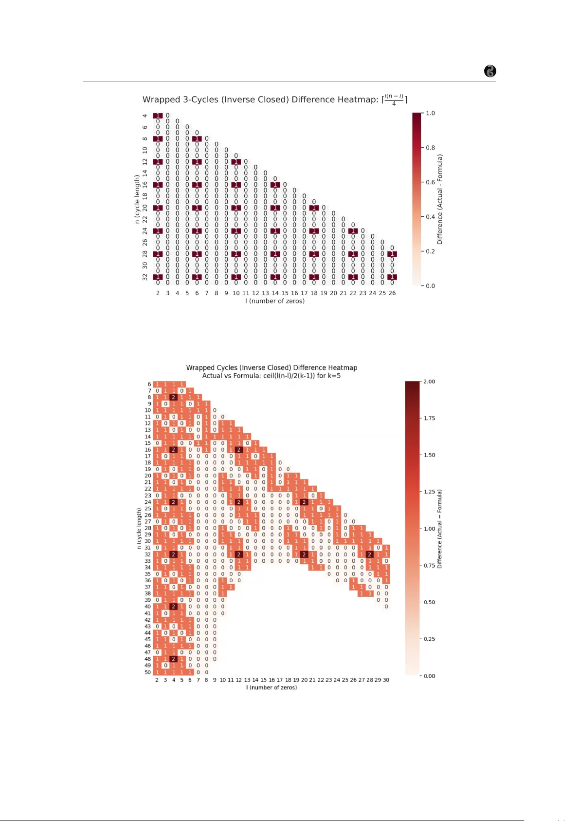
CA YLEYPY -4: AI-HOLOGRAPHY . TO W ARDS ANALOGS OF HOLOGRAPHIC STRING DU ALITIES FOR AI T ASKS. (PRELIMINAR Y VERSION) A. CHER V O V, F . LEVKO VICH-MASL YUK, A. SMOLENSKY, F . KHAFIZO V, I. KISELEV, D. MELNIK O V, I. K OL TSO V, S. KUD ASHEV, D. SHIL TSO V, M. OBOZO V, S. KR YMSKII, V . KIR O V A, E.V . K ONST ANTINO V A, A. SOIBELMAN, S. GALKIN, L. GR UNW ALD, A. KO TO V, A. ALEXANDR O V, S. L YTKIN, D. FEDORIAKA, A. CHEVYCHELO V, Z. K OGAN, A. NA TYR O V A, L. CHELDIEV A, O. NIKITIN A, S. FIRONO V, A. V AKHR USHEV, A. LUKY ANENK O, V . ILIN, D. GOR ODKO V, N. BOGACHEV, I. GAIUR, M. ZAITSEV, F . PETR O V, L. PETR O V, T . GAINTSEV A, A. GA VRILO V A, M. N. SMIRNO V, N. KALININ, A. KHAN, K. JUNG, H. MOUSSET, H. ISAMBER T, AND O. DEBEA UPUIS A B S T R AC T . This work is the fourth paper in the CayleyPy project, which aims to apply AI-based methods to large graphs. Here, we propose connections to a novel discretized analogue of holo- graphic string dualities originating in theoretical physics. W e argue that this perspecti ve can lead to more efﬁcient approaches to a wide range of AI tasks. Many modern AI problems—such as those addressed by GPT -style language models or rein- forcement learning systems—can be viewed as direct analogues of predicting particle trajectories on graphs. W e hypothesize that these tasks admit a holographically dual description in terms of discrete strings, and that working in this dual representation can provide a more tractable formu- lation of the original problems. In particular , strings - holographic images of states are proposed as natural candidates for embeddings, motiv ated by the “complexity = volume/action” principle in AdS/CFT . In a simple illustrative example, the R OC curv es serve as holographically dual strings to the nodes of some graphs. From a mathematical standpoint, we e xpect that all properties of graphs can be e xpressed entirely within this duality framew ork, yielding nontri vial identities. Furthermore, for Cayley graphs of the symmetric group S n , we conjecture that the corresponding dual objects are planar polygons and present various examples. Graph diameters equal the number of integer lat- tice points in the n -scaled polygon (Ehrhart quasi-polynomials). V ertices of graphs can be mapped (“holography”) to lattice paths inside the polygon in such a way that word metrics (“gate com- plexities”) are equal to the areas under the corresponding paths in accordance to “complexity = volume/action” principle. This thus pro vides an e xplanation for the quasi-polynomiality conjecture regarding diameters and word metrics from our pre vious paper . Stanley-type formulas for count- ing shortest paths can be reinterpreted as identities relating particle extremals on Cayley graphs to string extremals on the associated polygons. In some cases, the graph Laplacian coincides with integrable spin-chain Hamiltonians and yields conformal ﬁeld theories in the large-size limit. W e also study the corresponding H-polynomials and their properties, including positi vity , unimodality , duality , and analogues of the Riemann conjecture. Project page: https://github.com/CayleyPy/CayleyPy K ey wor ds and phrases. Machine learning, reinforcement learning, Cayley graphs. 1 CayleyPy-4: Holography CayleyPy collaboration C O N T E N T S 1. Introduction 3 1.1. Main hypothesis: particle-string holographic duality for AI-tasks 5 1.2. Guiding principle: “complexity = volume/action” 5 1.3. S n -Cayley graphs to planar polygon duality: lattice paths as discrete strings holographically dual to graph nodes 6 1.4. List of contributions 8 1.5. Organization of the paper 9 2. Simplest Examples. ROC curv e = string dual to Gr ( k, n ) graph node 11 3. AI tasks as predictions of particle trajectories. General AI-holography expectations 14 3.1. Particle trajectories as te xts or action sequences 14 3.2. AI-holography 18 3.3. Further remarks. 19 4. Case studies 19 4.1. S n Cayley graphs and polygon duality 19 4.2. CayleyPy AI methodology for assisting in determining the duality 23 4.3. S L (2 , Z ) and the F arey graph 24 5. Neighbor transpositions Cayley and Schreier graphs 26 5.1. Multiset { 0 n 0 1 n 1 . . . m n m } 26 5.2. Cosets with 0,1,2 components - alternativ e representation 27 5.3. Box-Ball System ev olution as a deterministic walk on a Schreier/Cayley graph and the A UC–AAC duality 29 5.4. Schreier graphs for orbits of tuples 31 5.5. Large size limits, to wards ”macroscopic” descriptions 33 5.6. V ershik’ s (1996) limit shapes for rectangular Y oung diagrams, general q 33 5.7. V ershik’ s (1985) limit shapes for rectangular Y oung diagrams q = 1 34 5.8. Limit shape for R OC-curves (Dyck paths) 35 5.9. Dynamics in large size limits. T ASEP-Burgers correspondence. KPZ. 36 5.10. Spanning trees for ﬁnite spin-up sector , 1/n expansion, Benjamini-Schramm limit to lattices, Mahler measures 38 5.11. Limit to ﬁeld theory string-like model. Spanning trees for many spins up and do wn sector 45 6. Neighbor transpositions extended by (0 , n − 1) (“wrapped” or “afﬁne” case) 49 6.1. Duality for the Wrapped Case 49 6.2. Diameters for the Schreier coset graphs “few-coincide”: S n /S d 51 7. Bethe ansatz and graph spectrum 52 7.1. Spectral gap 53 7.2. Relation to Laplacian spectrum 53 7.3. Schreier graph with non-wrapped 2-cycles 53 7.4. Relation between Schreier and Johnson graphs 54 8. Consecutiv e-(k)-cycles. Quasi-polynomiality , etc. 55 8.1. Section outline 55 8.2. ( k − 1) -Shrinkage heuristics: Results and Difﬁculties 55 8.3. Theoretical lower and upper bounds on the diameters. Cayley graphs. 55 8.4. Theoretical diameters estimate. Schreier coset graphs S n /  S ⌊ n/ 2 ⌋ × S n −⌊ n/ 2 ⌋  56 8.5. Quasi-polynomials for diameters. Cayley graphs. 57 8.6. Schreier coset graph: S n /  S ⌊ n/ 2 ⌋ × S n −⌊ n/ 2 ⌋  (not in verse-closed) 62 8.7. Schreier coset graph: S n /  S ⌊ n/ 2 ⌋ × S n −⌊ n/ 2 ⌋  (in verse-closed) 65 8.8. Schreier coset graph: S n /  S l × S n − l  (“ k -shrunken” Grassmannian Gr ( l, n, k ) ) 74 8.9. Schreier coset graph: ”few coincide” 76 8.10. Schreier coset graph: ”L-Different” in verse closed 82 8.11. W ord-metrics for [012]-repeated full ﬂips, 3-cycles 86 9. Wrapped (”afﬁne” or ”periodic”) (k)-consecuti ve cycles. Quasi-polynomiality , etc. 88 9.1. Section outline 88 9.2. 2( k − 1) -Shrinkage heuristics: Results and Difﬁculties 88 9.3. Theoretical diameters estimate. Schreier coset graphs S n /  S ⌊ n/ 2 ⌋ × S n −⌊ n/ 2 ⌋  88 2 CayleyPy-4: Holography CayleyPy collaboration 9.4. Schreier coset graph: S n /  S l × S n − l  (“ k -shrunken” af ﬁne Grassmannian Gr af f ( l, n, k ) ) 89 9.5. Schreier coset graph: S n /  S ⌊ n/ 2 ⌋ × S n −⌊ n/ 2 ⌋  (not in verse-closed) 91 9.6. Schreier coset graph: S n /  S ⌊ n/ 2 ⌋ × S n −⌊ n/ 2 ⌋  (in verse-closed) 98 9.7. Some eccentricities for Schreier coset graph: S n /  S ⌊ n/ 2 ⌋ × S n −⌊ n/ 2 ⌋  101 9.8. W ord metrics to full ﬂips for Cayley and Schreier ( S n /S d ) graphs 106 9.9. Coset 2-different 115 9.10. Coset 3-different 116 9.11. Coset 4-different 121 10. Reminder . Background and related works 122 10.1. Cayley and Schreier graphs, diameters, gro wth 122 10.2. Quasi-polynomial functions 124 10.3. Ehrhart polynomials 124 10.4. R OC curves and A UC 125 Acknowledgments 128 References 129 1. I N T RO D U C T I O N The deep learning re volution is one of the most exciting scientiﬁc breakthroughs of our time. The second superstring rev olution [ W itten1995 ; Schwarz1996 ] was one of these in the past. The present paper takes a step tow ard merging these two. The theme of duality is one of the central ideas in theoretical physics: the belief that for many complex systems there exists a “dual” descrip- tion in which questions that are difﬁcult in the original (“strong-coupling”) formulation become simpler in the dual (“weak-coupling”) one (e.g. [ Polyako v1987 ]). In particular , the AdS/CFT holographic duality [ Maldacena1998 ] marked the culmination of the second superstring rev olu- tion with the disco very of the long-sought duality between gauge theory and string theory , and has since become the most cited paper in high-energy theoretical physics. Here, we present evidence that a similar principle may apply to artiﬁcial intelligence tasks, arguably leading to more ef ﬁcient approaches than those currently av ailable. W e draw a parallel between dualities in physics and the concept of embedding (“latent represen- tation”) in cognitiv e theory , both for natural and artiﬁcial neural netw orks. The role of embeddings in AI is analogous to the notion of duality in physics: they transform an input representation, in which semantic relations are difﬁcult to analyze, into a representation where these relations be- come more tractable. A well-kno wn example in ML is the relation ”king - man + woman = queen” ( W ord2vec [ Mik olov2013 ]), where a nontri vial semantic relationship is mapped to a simple vec- tor arithmetic operation. Finding appropriate embeddings is a central problem in modern AI. W e argue that the perspecti ve of the AdS/CFT correspondence offers a ne w conceptual frame work for approaching this problem. Brief outline of the main ideas. (1) Setup. The starting point is that AI tasks such as language or RL modeling can be vie wed as particle trajectory prediction tasks on edge-labeled graphs. (2) W e hypothesize that in many cases such particle systems admit a holographically dual string de- scription (in the spirit of AdS/CFT), conv erting difﬁcult problems into more tractable ones. W e outline how this can be used to build more effecti ve AI systems: embeddings (”latent representa- tions”) are strings, training is based on the ”complexity = v olume” principle in AdS/CFT . From the mathematical viewpoint, we expect that all properties of graphs can be seen from the dual side, as is typical in string dualities, leading to new mathematical insights. (3) For the case of S n Cayley graphs, we present signiﬁcant evidence that the dual objects are planar rational polygons, and that holography maps nodes of the graphs to lattice paths (discrete strings) inside the poly- gons. W e also present connections to various deep questions and conjectures in mathematics. (4) As simplest e xamples, R OC curves (Dyck paths) can be used to illustrate the ideas in a clear and straightforward manner . 3 CayleyPy-4: Holography CayleyPy collaboration Surprisingly , the simplest example – which is just the Cayley (Schreier) graph generated by neighboring transpositions – is connected to sev eral advanced areas of research: quantum inte- grable systems and the Bethe ansatz (since the graph Laplacian coincides with the Hamiltonian of the Heisenberg spin chain), Mahler measures (related to supersymmetric Landau–Ginzburg models and mirror symmetry for Fano varieties ) for counting spanning trees, Burgers and Kar- dar–Parisi–Zhang ( KPZ ) equations for description of geodesic ﬂow in a dual formulation for lar ge size, limit shapes of Y oung diagrams, Beilinson’ s conjectures on special values of L -functions, and more. Moreo ver , we propose that conformal ﬁeld theory arising in large size limit for such graphs is dual (in AdS/CFT manner) to a simple free scalar with radius of compactiﬁcation related to normalized area of the dual polygon (in this case it plays the role of the dual ”string”) and propose conjectures on spectrum of conformal dimensions. Let us present a more detailed outline. (1) AI as particle on edge-labeled graphs . AI tasks in volving languages or reinforcement learning can be naturally interpreted as problems of predicting particle dynamics on edge- labeled graphs (for instance, Cayley graphs). The data — texts or sequences of actions — correspond to particle trajectories, that is, sequences of traversed edges. Such edge (”token”) sequences naturally deﬁne the corresponding “te xts. ” T ypical tasks then amount to determining the trajectory given initial (the ”prompt” for generativ e models) or bound- ary conditions (the ”masked language modeling objective” for e.g. BER T or ”win the game/reach the goal” in RL). (2) Particle-string holographic duality . W e hypothesize that many such tasks admit a holo- graphically dual equiv alent description in terms of discrete string theory , transforming a dif ﬁcult problem on the original graph-side (”CFT -side”) into a more tractable one on the dual string-side (”AdS-side”), in the spirit of strong–weak coupling duality , thus giving a key to build more efﬁcient AI-systems. This perspectiv e is inspired by the landmark AdS/CFT correspondence. W e further ar gue that strings (vie wed as holographic duals of states) provide natural candidates for embeddings (latent representations), and that un- con ventional (“tropical”) string actions may be required to capture phenomena intrinsic to discrete settings. W e remark that “embeddings, ” whether in natural or artiﬁcial neural systems, play a role analogous to “duality” in physics: they transform input data into repre- sentations that are more tractable than the original formulation. The celebrated AdS/CFT principle ”complexity = volume/action” can be used as a training objective for string em- beddings, and also plays many other ke y roles. From a mathematical point of view , we expect that all properties of the graph admit a complete description in terms of the dual theory , as it is typical in string dualities. This dual perspecti ve may provide ne w results and structural insights, some of which are presented here. W e suggest v arious connec- tions with integrable systems, matrix models, conformal ﬁeld theory , cluster algebras, the thermodynamic Bethe ansatz, and related structures. (3) S n Cayley graphs / planar polygon duality . In the case of Cayley graphs of the per- mutation group S n , we propose that the holographically dual objects are planar rational polygons. The holographic correspondence maps graph nodes to lattice paths (discrete strings). Diameters and word metrics can then be described in terms of Ehrhart quasi- polynomials of the associated polygons or of their subregions (e.g. areas under lattice paths), thus explaining the quasi-polynomiality conjecture from our previous paper . This is consistent with the “complexity = volume/action” principle from AdS/CFT : complex- ities coincide with word metrics in Cayley graphs, while counting lattice points corre- sponds to discretized v olumes. Using the CayleyPy AI-based library and methodology , we obtained v arious results and conjectures concerning the corresponding quasi-polynomials and related H -polynomials. That is, we compute “complexities” and demonstrate their agreement with the corresponding “volumes. ” 4 CayleyPy-4: Holography CayleyPy collaboration (4) Simplest examples. R OC-curves (Dyck like paths) as strings. As a starting point, we present simple and explicit examples in which classical R OC curves can be interpreted as discrete strings holographically dual to nodes of an appropriate graph. Sev eral combina- torial facts then admit a natural interpretation in terms of discrete string duality . Surpris- ingly , ev en this simple example is connected to deep recent mathematical results, and in fact touches upon se veral open problems. 1.1. Main hypothesis : particle-string holographic duality for AI-tasks. The AdS/CFT holo- graphic duality [ Maldacena1998 ] predicts that difﬁcult questions on the CFT side (”strong cou- pling”) can be computed via more tractable geometric methods on the AdS side (where string theory at ”weak coupling” reduces to gravity). W e hypothesize the existence, outline expecta- tions and elaborate se veral examples of a similar holographic duality in the context of graphs, languages, and reinforcement-learning “en vironments” — systems of interest in artiﬁcial intelli- gence, mathematics, and physics. First, we emphasize that many such settings can be viewed as particle trajectories on edge-labeled graphs (e.g. Cayley graphs ), where the trajectories deﬁne a “language, ” i.e., sequences of admissible tokens/moves. Second, we hypothesize that a “particle” moving on such graphs may admit a holographically dual description as a (discrete) “string” living on an appropriate dual object. If such a duality e xists, the string description may be more tractable (analogous to a weak-coupling regime) and could provide a key to constructing more powerful AI models. In particular we expect that strings understood as holographic images of states may provide ”good embeddings”. Our examples suggest that one should consider unusual (“tropical”) analogues of discrete string actions that inv olve functions of the form max( · , 0) (also known as ReLU ). Such terms ensure that, ev en after ﬁxing initial or boundary conditions, the equations of motion retain substantial local freedom in their solutions — a feature that appears necessary for describing discrete setups. From a mathematical perspective, we e xpect that the properties of a graph (or the associated language, etc.) may be computable from the dual object, potentially leading to non-trivial identities and ne w structural insights. In particular , various combinatorial results might be reinterpreted as manifestations of string dualities. If indeed true as stated, our proposal would imply that string-theoretic holographic dual de- scriptions, in the sense outlined abov e, may exist for a wide range of AI systems. Examples of this could potentially include even such settings as English and other natural languages; programming languages; robotic manipulator systems; mathematics viewed as a formal proof system; games such as Go, chess, etc.; the languages of life (admissible protein and DN A sequences); chemical molecules encoded in databases; and so on. One may e ven ar gue that one reason a duality or sim- pliﬁcation of this kind might e xist for e.g. English language is that we indeed can learn it! Both humans and machines master it, which would be impossible without ability to con vert information to some latent representation where complex semantic relations can be seen via simple operations (which is the basically the duality: complex to simple). Our current proposal is more subtle: we expect that duality may be holographic in the spirit of AdS/CFT and that these efﬁcient latent representations (”embeddings”) could be interpreted as strings – that is, as holographic images of states (sentences in this case). Downstream computations performed on these embeddings may naturally inv olve Riemannian metrics –reminiscent of the AdS metric – while more subtle phe- nomena could correspond to ﬁnite-size corrections. More broadly , this perspective may e ven lead to a deeper geometric understanding of ke y concepts in AI. 1.2. Guiding principle: “complexity = volume/action”. The celebrated AdS/CFT principle “complexity = volume/action” (L. Susskind et al: [ Stanford2014 ; Bro wn2016 ]), together with subsequent works (including [ Lin2019 ] and work by one of the present authors, D. Melnikov , [ Camilo2019 ]) that bridge this idea with Cayley graphs , serves as one of the key insights and guiding framew orks for what follows. In the graph-theoretic setting, complexity admits a very simple interpretation. The complexity of one node with respect to another is deﬁned as the length of the shortest path between them in the graph. Then the ”complexity=volume/action” (abbrevi- ated to ”C=V/A” belo w) principle becomes a particular manifestation of particle-string duality . 5 CayleyPy-4: Holography CayleyPy collaboration Indeed, the extremal action of a particle – namely , the length of the shortest path – can be directly vie wed as ”complexity”. According to the duality principle, it should be equiv alent to the e xtremal action of the corresponding string worldsheet, which is naturally related to a volume-type quantity . Let us list a few other reasons this principle is important for us. One key point is that estab- lishing the duality itself is not e xpected to be a trivial task, e ven for relativ ely simple graphs. In contrast, results supporting the ”complexity = v olume/action” principle appear to be more acces- sible, and in some cases ev en numerical simulations can provide valuable insight. In particular , the primary goal of the CayleyPy project is to develop AI-based tools to estimate “comple xities” (i.e. lengths of shortest paths) using modern machine learning methods. Pre vious papers in the project hav e already achie ved state-of-the-art results in this direction. Moreover , one of the ke y conjectures formulated in our earlier work is that the “complexities” (diameters and word met rics) for S n -Cayley graphs are quasi-polynomials in n . In the present paper, we propose an extension of this conjecture: we observ e that these quasi-polynomials appear to be closely related to Ehrhart quasi-polynomials of certain planar polygons. This conjecture can be viewed as a manifestation and reﬁnement of the “C=V/A ” principle for S n -Cayley graphs, since it identiﬁes complexities with the number of lattice points in corresponding polygons. These lattice point counts may be interpreted as discrete “volumes, ” or “volumes” with ﬁnite-size corrections. Another reason is that the principle “C = V/A” can itself be viewed as a manifestation of a strong–weak coupling duality . Computing complexity for lar ge systems (such as graphs) is typ- ically extremely difﬁcult—often NP-hard—whereas the computation of geometric quantities like volumes is comparativ ely more tractable. In this way , a complicated problem is translated into a simpler one through a dual description. This perspectiv e also underlies our proposal to in- terpret strings (i.e., holographic images of states) as good embeddings (latent representations). The primary goal of embeddings—whether in natural neural networks or artiﬁcial systems—is to transform an original representation of information into a more tractable format, so that questions which are dif ﬁcult in the original representation become easier in the embedding space. From this vie wpoint, the principle “C = V/A” can be seen as predicting precisely such a mechanism: by representing states through strings, one effecti vely moves to a dual geometric description where complexity-lik e quantities become accessible through simpler geometric computations. W e pro- vide a more detailed discussion of this perspecti ve in the main text. In the present work, we use the term “area” rather than “volume”, since our examples are pla- nar . W e also typically use other terms instead of “complexity , ” which are more standard in graph theory . Often, a distinguished reference node is chosen—such as the identity element in the case of a Cayley graph—and the complexity of all other nodes is measured relati ve to this reference. In group-theoretic language, this notion is known as the word metric . In coding theory and bioinfor- matics, it is related to metric codes and e volution metrics and mutations, respectiv ely (see [ Kon- stantinov a2008 ] for more details). In computer science, it is closely related to circuit complexity , while in quantum computing it appears as quantum gate complexity , quantifying the minimal num- ber of elementary gates required to generate a gi ven element. Complexity optimization is one of the central challenges in quantum computing [ Nam2018 ; Ruiz2025 ], while the computation of word metrics is a fundamental problem in computational group theory . Previous papers from the CayleyPy project [ Chervov2025c ; Chervo v2025a ; Chervo v2025b ] hav e provided state-of-the-art solutions to this problem. 1.3. S n -Cayley graphs to planar polygon duality: lattice paths as discrete strings holo- graphically dual to graph nodes. The present paper elaborate the conjectures for S n -Cayley and Schreier graphs. W e propose that the corresponding dual objects are rational planar polygons (or line se gments in de generate cases). The holographic map associates each node of the graph with a lattice path on the dual polygon. Our central conjecture is that the diameter of the graph equals the number of integer lattice points in the polygon, while more generally , the word metric of any node corresponds to the area under its associated lattice path. Consequently , both diameters and word metrics can be described as Ehrhart quasi-polynomials of the n -rescaled polygon, providing a 6 CayleyPy-4: Holography CayleyPy collaboration natural explanation for the quasi-polynomiality conjecture in our previous work [ Cherv ov2025b ]. These conjectures can be viewed as reﬁnements of the “complexity = area” principle, since word metrics—interpreted as computational complexities—are predicted to correspond directly to areas under the dual lattice paths. The planarity of those polygons is conditioned to the celebrated 50+ years old open problem [ Rubtsov1975 ] (revie ws [ Glukhov1999 ], [ Helfgott2013 ]) that diameters of S n Cayley graphs are bounded by n 2 . The conjecture can be a seen a special case of the L.Babai conjecture on diameter of any ﬁnite simple group, for which certain progress has been achieved by T .T ao et.al. Still both conjectures are widely open, ev en establishing a polynomial bound is not achie ved. For further discussion and reﬁnements, we refer to [ Chervo v2025b ] and discussions below . Each quasi-polynomial has a naturally associated H -polynomial, that is simply the numerator of the generating function, which coincides with the Poincar ´ e polynomial of the corresponding toric v ariety under appropriate smoothness assumptions. Important questions in combinatorics are whether these H -polynomials satisfy the same properties as those arising from ”good” toric v arieties, namely: positivity , duality (Poincar ´ e symmetry), unimodality , and an analogue of the “Riemann conjecture” (i.e., that all roots lie on the unit circle). In the present paper , we compute v arious H -polynomials associated with diameters and word metrics, and inv estigate their prop- erties, formulating a number of conjectures. In some cases, all of the expected properties hold; ho wev er , in other situations we observe that each of them may be violated. The cases of the Cayley graphs with neighbor transposition (Coxeter) generators of S n are the most classical ones. W e present quite an detailed picture of the dualities here. The holography map can be described by e.g. Lehmer codes or by related constructions e.g. R OC-curves. ”Complex- ity = Area” reduces to kno wn statements that areas under the R OC-curves correspond to Mann- Whitney statistics, and similar statements for the Lehmer codes. Bijectiv e description of shortest paths on these graphs [ Stanley1984 ; Edelman1987 ] can be interpreted as bijections between the extremals of a particle and the corresponding strings, in accordance with the conjectured dual- ity . In this frame work, extremal string worldsheets are naturally associated with Y oung tableaux. String action is ”tropical” (or ”ReLU”) analogue of the conv entional string action. Graph Lapla- cians can be identiﬁed with the Hamiltonians of Heisenberg XXX spin chains. Etc. The other cases studied in the present paper are generalizations of neighboring transpositions to k -neighbor versions, such as k -consecuti ve cycles of the form ( i, i + 1 , i + 2 , . . . , i + k − 1) and their v ariations. W e present evidence that, in this setting, the results can be described by a ( k − 1) -shrinkage prin- ciple: namely , the quantities (in particular dual polyygons) in the standard case should be rescaled by ( k − 1) to obtain the corresponding results in the general case, at least at the lev el of leading terms. W e present various conjectures on diameters, word metrics, as well as the corresponding quasi-polynomials and H -polynomials in these generalized settings, obtained with our CayleyPy library . In general, determining the dualities and the corresponding dual polygons is a highly nontri vial task. Already the computation of diameters and w ord metrics is well known to be dif ﬁcult in its o wn right. Our approach is based on the CayleyPy library , in particular on its AI component. The heuristic strategy for identifying dual polygons is as follows. First, we attempt to determine quasi-polynomials for the diameters. Second, we try to identify polygons whose Ehrhart quasi- polynomials match the observ ed data. T o determine diameters, we proceed in se veral steps. Using ef ﬁcient implementations within CayleyPy , we perform brute-force computations of diameters for the ﬁrst sev eral v alues of n , and we identify the corresponding longest elements (states). Next, we attempt to detect patterns in these longest states and formulate conjectural descriptions valid for all n . If this step is successful, we then use the AI component of CayleyPy to compute word metrics of these candidate longest states, which allo ws us to reach signiﬁcantly larger v alues of n than are accessible by brute force alone. W ith sufﬁciently e xtensiv e data at hand, we ﬁt quasi-polynomials for the diameters and compare them with Ehrhart quasi-polynomials of suitable polygons. W e demonstrate that this approach is successful in a number of cases. 7 CayleyPy-4: Holography CayleyPy collaboration 1.4. List of contributions. Let us outline contrib utions of the present paper in the itemized form, which mainly follo w the order of the exposition: • Simplest examples. ROC curve (Dyck like paths). Surprisingly , the basic quality met- rics in machine learning such as the R OC curve and ROC-A UC score can be used to illustrate our holographic duality for graphs in a very simple and explicit way . In this frame work, R OC curves (which are quite similar to Dyck paths ) are strings “holograph- ically dual” to nodes of a certain class of graphs. ( S n / ( S k × S n − k ) or ”Grassmanians” ov er ”ﬁeld with one element. ”) Within this setting, the analogue of the AdS/CFT relation “complexity = area” reduces to the familiar equality between the Mann–Whitney statistic and the area under the R OC curve. Bijecti ve description of shortest paths on these graphs [ Stanley1984 ; Edelman1987 ] can be interpreted as bijections between the extremals of a particle and the corresponding strings, in accordance with the conjectured duality . In this frame work, extremal string worldsheets are naturally associated with Y oung tableaux. String action is ”tropical” (or ”ReLU”) analogue of the con ventional string action. Graph Laplacians can be identiﬁed with the Hamiltonians of Heisenber g XXX spin chains. The number of spanning trees is related to the Mahler measure, in accordance with general expectations. W e also present an analysis of the limit shapes of ROC curves and outline se veral open questions. • Charting general holographic duality f or AI. W e hypothesize that for many graphs and corresponding AI-systems (languages, and RL-en vironments) there are dual objects whose features include: – Holography . [ Hooft1993 ; Susskind1995 ] Meaning that d -dimensional objects on graph side are mapped to ( d + 1) -dimensional ones on the dual side. I.e. graph nodes to paths (”strings”) on the dual side, paths on graph to 2-dimensional objects - like Y oung tableaux (”string worldsheets”). W e expect that the strings which are holographic images of states and ”good embeddings”. – Particle on the graph side (“CFT”-side) = Discrete String on dual side (“AdS”- side). As is typical in string dualities, we e xpect that a theory deﬁned on one side is equi valent to a theory deﬁned on the other side, and our proposal consists of duality between particle theory and string theory . – Corollary: Complexity = Area/Action. This is a consequence of the previous prin- ciple: values of action for particles on extremals are lengths of the shortest path, while for the string these are related to certain areas. – Strong coupling to weak coupling. As in con ventional string theory , we expect that dif ﬁcult problems on the original side are con verted into more tractable problems on the dual side. In particular we expect that strings dual to nodes of the original graph provide ”good” embeddings (from AI point of vie w). • Case studies and mathematical conjectures. W e outline sev eral concrete examples of duality for Cayley graphs. W e explain its relation to quasi-polynomiality hypothesis and the n 2 conjectural bound for diameters of S n Cayley graphs, which is a celebrated open problem in mathematics for more than 50 years. W e explain ho w CayleyPy AI methodol- ogy assists in determining the duality . W e discuss other examples related to SL(2 , Z ) and Fare y graphs, etc. – S n -Cayley to planar polygon duality . For S n - Cayley and Schreier graphs, we con- jecture that the dual objects are rational polygons in the plane (or , in degenerate cases, line segments) such that the graph diameter equals the number of integer lattice points in the n -scaled polygon. This provides an illustration of a reﬁned version of the “complexity = area” principle in this context. In other words, diameters are given by the Ehrhart quasi-polynomials of the polygons, explaining the conjecture from our 8 CayleyPy-4: Holography CayleyPy collaboration pre vious work. Such a relation is far from trivial: in particular , it implies the cel- ebrated open problem predicting that the diameters of these graphs are bounded by n 2 , a conjecture that has resisted the ef forts of leading mathematicians for decades [ Rubtsov1975 ] (re vie ws [ Glukhov1999 ], [ Helfgott2013 ]). – Holography: nodes to lattice paths; word-metrics quasi-polynomiality . In this frame work, ”holography” predicts that vertices of the graph can be mapped to lattice paths inside the polygon in such a way that word metrics (or “gate complexities”) coincide with the areas under the corresponding paths. This again mirrors the “com- plexity = area” principle familiar from AdS/CFT , and implies that word metrics are also described by Ehrhart quasi-polynomials, e xplaining the conjecture from [ Cher- vo v2025b ] that word metrics are quasi-polynomials in n for S n . – Holography = Lehmer code (f or Coxeter generators graphs). For Cayley graphs generated by neighboring transpositions, such a mapping is closely related to the Lehmer code . – CayleyPy AI-methodology to ﬁnd diameters and wordmetrics. W e present a methodology how we can ﬁnd diameters using our AI-based CayleyPy library , and present multiple successful examples of computations discussed before are based on it. – Behavior under taking G/H . Empirically , we observe the following pattern: the polygon associated with the Schreier coset graph of G/H appears as a subpolygon of the polygon corresponding to Cayley graph of the full group G . – Consecutive k -cycles and variations — ( k − 1) -shrinkage principle. W e present se veral computations of diameters and word metrics for generators giv en by con- secuti ve k -cycles, explicitly obtaining the corresponding quasi-polynomials. Em- pirically , we observe that these formulas approximately correspond to shrinking the graph ( k − 1) times, a behavior that is particularly reﬂected in the associated dual polygons. – SL(2 , Z ) and F arey graphs. W e put into the frame work of the present paper results from the pre vious paper by one use: (D.Melnikov et.al. [ Camilo2019 ]). – Properties of the corresponding H -polynomials. T o each quasi-polynomial, one naturally associates an H -polynomial, and we study their properties. In many cases, we observe positivity , unimodality , Poincar ´ e duality , and analogues of the Riemann conjecture. While some examples satisfy all of these properties, there are cases in which one or more of them are violated. – Limit shapes. W e study the limit shape of the corresponding ”strings” in lar ge size limit, on the example of the Coxeter group, we proposed exact formulas for limit shapes with ﬁxed areas under the curves, which are consistent with pre vious results by A.M.V ershik et.al. – Evolution in large size limit, Burgers equation and KPZ. W e study numerically the geodesic ﬂow on the graph in the dual picture and conjecture its relation with Burgers and KPZ equations. – Spanning tr ees, Mahler measur es, string-lik e model with polygonal w orldsheets, spin chains in thermodynamic limits, spectra of conformal dimensions. W e study Laplacian and spectral properties in large size limits. W e propose various conjectures on numbers of spanning trees. W e also propose identiﬁcation of limitings theories with a free bosonic model (playing here the role of a string-like dual) which surpris- ingly may ha ve polygonal worldsheets. The conformal dimensions of primary ﬁelds are conjectured to be eigen v alues of the Laplacian on the dual planar polygon. 1.5. Organization of the paper. The ﬁrst ﬁve sections present the main examples and core ideas, while the remaining sections provide further details and technical computations. Although the ov erall length of the paper is substantial, we hope that the ﬁrst ﬁ ve sections are sufﬁcient for the 9 CayleyPy-4: Holography CayleyPy collaboration reader to grasp the central concepts and motiv ation. W e put reminders on background material to the last section. AI, mathematics and physics The second superstring rev olution and related de velopments rev ealed highly nontrivial du- alities among string-related theories and uncovered far-reaching consequences [ Candelas1991 ; Seiberg1994 ; W itten1995 ; Polchinski1995 ; Schw arz1996 ; Strominger1996 ; V afa1996 ; Strominger1996 ; Banks1997 ; Connes1998 ; Maldacena1998 ; Gubser1998 ; W itten1998 ; Kontse vich2003 ; Catta- neo2000 ; Gross2000 ; De Boer2000 ; Dijkgraaf2002 ; Nekrasov2003 ; Minahan2003 ; Okounko v2003 ; Ooguri2004 ; Gukov2005 ; Dabholkar2005 ; Ryu2006 ; Kapustin2007 ; Pestun2012 ; Mironov2010 ; Alday2010 ; V erlinde2011 ; Gaiotto2013 ; Stanford2014 ; Grassi2016 ; Gaiotto2015 ; Bro wn2016 ; Hijano2016 ]. These de velopments hav e profoundly inﬂuenced the e volution of modern mathe- matics in a variety of directions. W e hope that the dualities proposed here may e xtend the scope of string-theoretic ideas to new domains, including artiﬁcial intelligence, as well as to such areas of mathematics such as graph theory , group theory and combinatorics. One of the ”pre-AdS/CFT” ex- amples of dualities w as proposed for two-dimensional Y ang-Mills (its string description, ”Gross- T aylor formula”) [ W itten1992 ; Gross1993b ; Gross1993a ; Cordes1995 ], recently it has been con- nected to Cayley graphs via ”Y ang-Mill/Hurwitz correspondence” [ Nov ak2024 ], moreover quasi- polynomial expressions which play ke y role in the present paper , also appear in Hurwitz theory [ Norbury2010 ; Andersen2018 ; Kramer2020 ], it would be tempting to understand relations to the present paper . The present time is characterized by growing interest in and number of applications of deep learning methods to mathematics and physics: machine learning has been emerging as “a tool in theoretical science” [ Douglas2022 ]. In recent years, this has led to several notew orthy ap- plications to mathematical and physical problems: [ Lample2019 ; Davies2021 ; Bao2023 ; Romera- Paredes2024 ; Coates2023 ; Alf arano2025 ; Charton2024 ; Shehper2024 ; Swirszcz2025 ; Hashemi2025 ; He2024 ; Lal2024 ; Lal2025 ; Douglas2025 ; Georgie v2025 ; Berczi2026 ; Ju2026 ; Gue vara2026 ; El- lenberg2026 ; Chen2026 ; Knuth2026 ; Morozov2026 ]. Seewoo Lee created a repository that col- lects papers in AI for mathematics, A wesome AI for Math . The present paper can be seen as an attempt at a dual-sided application of AI to mathematics and physics, and vice versa. 10 CayleyPy-4: Holography CayleyPy collaboration 2. S I M P L E S T E X A M P L E S . R O C C U RV E = S T R I N G D U A L T O Gr ( k , n ) G R A P H N O D E F I G U R E 1 . Left to right: the graph Gr 2 , 5 with marked vertices (red and green), and a polygon illustrating the corresponding paths (red and green). F I G U R E 2 . Left to right: the graph Gr 2 , 6 with marked vertices (red and green), and a polygon illustrating the corresponding paths (red and green). Interactiv e widget (F .Khaﬁzov) av ailable at link . The distance between nodes on graph is equal to area between the paths - ”complexity = area” principle. Which in that case is equality of the Mann–Whitne y statistic and the area under the R OC curve. Section Outline. Here we present the basic example for the main ideas of the present paper . W e consider a simple Cayley graph and describe the duality for it. R OC curves (Receiv er Operating Characteristic curves) and area under the R OC curves are widely used quality metrics in ML. (See e.g. the exposition by A. G. Dyakono v , ﬁrst Kaggle top-1 Grandmaster .) Surprisingly , these e xamples can be used to illustrate the idea of holographic string duality , as well as to highlight various non-trivial results and open questions. The “complexity = area” principle reduces here to the familiar equality between the Mann–Whitney statistic and the area under the R OC curve. Figures 1 , 2 illustrate the discussion below . So we describe below two sides of the correspondence: the graph (“CFT -side”) and the rectangle polygon (“ AdS-side”); the map from graph nodes to paths on rectangle (“holography map”). W e demonstrate its simple, but non-trivial properties which can be summarized a “particle on a graph dual to a string on the rectangle”. The discrete string has an simple action which is a ”tropical” (”ReLU”) analogue of the conv entional action. The explanations ho w it is applied in ML tasks as a quality metric are also provided. 11 CayleyPy-4: Holography CayleyPy collaboration Graph. “CFT -side”. Graph nodes correspond to vectors of length n with entries k zeros and n − k ones. T wo nodes are connected by an edge if there is a transposition of some neighbor elements ( i, i + 1) which sends one vector to the other one. This graph is the Schreier coset graph for S n with neighbor-transposition generators; it is a quotient of the permutohedron graph by S k × S n − k and should be thought of as the Grassmanian Gr ( k, n ) = GL ( n ) / ( GL ( k ) × GL ( n − k )) ov er the ﬁeld with one element , by the usual analogy S n = GL n ( F 1 ) . Polygon = rectangle. “AdS-side”. Consider the rectangle of the size k × ( n − k ) on the plane with integer coordinates. Set of our paths (“strings”) are paths making steps right and up going from (0 , 0) to ( k , n − k ) . These are similar to Dyck paths , but there is no restriction for them to be under the diagonal. “Holography map” from graph nodes to paths (“strings”). T ake a vector of 0’ s and 1’ s and associate to it a path by the rule: each “1” is a step up, each “0” is a step right. Clearly it is a bijection from graph nodes to paths described above. As we will discuss belo w these are precisely the R OC curves for certain machine learning models. “Complexity = ar ea”. Mann-Whitney = area under the R OC curve. T ake tw o nodes on the graph and consider the distance between them, i.e., length of the shortest path, or , equi valently , the minimal number of neighbor transpositions which are needed to transform one vector to the other one (“gate complexity”). One can check: Proposition 1. For any two nodes the distance between them on the graph (i.e. the complexity of one with respect to the other) is equal to the area between corresponding paths. T ypically as one of the nodes we take the sorted vector 0 ... 01 ... 1 , which corresponds to the path going along the bottom-right border . So in that case we get that the area under the curve equals the complexity of the other node. Use in ML. Notation abuse of “under” vs. “above” the cur ve. Consider a binary classiﬁca- tion task with n observ ations, of which k hav e ground-truth label 0 and n − k have label 1 . A machine-learning model assigns a probability score to each observation. Sorting the observations by these scores produces an ordered binary v ector consisting of zeros and ones (ground truth la- bels). For a perfect model, this vector is 0 k 1 n − k (i.e. it is sorted). An imperfect model produces a non-trivial interleaving of zeros and ones. Any metric that quantiﬁes deviation from the per- fectly sorted vector therefore can serve as a natural measure of model quality . One such metric is obtained by encoding the binary vector as a lattice path, as described abov e. The area under this path provides a quantitati ve measure of de viation from the perfectly sorted v ector 0 k 1 n − k . Indeed, the lattice path corresponding to that vector is the bottom-right boundary of the corresponding rectangle and hence has zero enclosed area. Proposition 1 shows that this measure has a natural combinatorial interpretation: it equals the minimal number of neighboring transpositions required to transform the giv en vector into the sorted one. This is precisely the statistic introduced by Mann, Whitney , Wilcoxon, and Kendall in classical rank-based hypothesis testing, and it admits modern group-theoretic interpretations as dev eloped in foundational work by P . Diaconis (see, e.g., [ Chat- terjee2016 ] and references therein). W e note a minor ab use of terminology: in our con vention, the area under the path measures deviation from the perfectly sorted vector , whereas in the standard R OC-curve exposition, the area under the curve measures similarity to the ideal classiﬁer . Our choice of con vention aligns naturally with the guiding principle “comple xity = area”. Stanley–Edelman–Greene corr espondence as a bijection of extremals f or a particle on a graph and strings on a polygon. [ Stanley1984 ] computed the number of shortest paths between the two most distant vertices of the permutohedron graph; such paths are known as sorting networks . As discussed in the inﬂuential paper Random Sorting Networks [ Angel2006 ]: “another breakthrough w as achie ved by Edelman and Greene” [ Edelman1987 ], who constructed a bijection between sorting networks and staircase-shaped standard Y oung tableaux of size n . W e now formulate an analogue of this result for our graph and provide its string theory interpretation. 12 CayleyPy-4: Holography CayleyPy collaboration Proposition 2. Let A and B be two vertices of the graph abov e. Then the shortest paths between A and B are in bijection with Y oung-type tableaux associated with the re gion bounded by the corresponding holographically dual lattice paths. Discrete string action whose extr emals are Y oung tableaux: standard + ReLU . The simplest continuum string action is R R  X 2 a + X 2 b  da db . In the discrete setting, deri va- ti ves are replaced by ﬁnite differences, X a = X ( a, b ) − X ( a + 1 , b ) , X b = X ( a, b ) − X ( a, b + 1) . Consider the discrete action: P a,b  ReLU( X a ) + ReLU( X b )  , where ReLU = max( · , 0) is ReLU function. It follows that the minima of this action are precisely Y oung tableaux, i.e. they provide solutions for equations of motion; at the same time, the action closely resembles that of a con ventional string theory . Corollary . (Stringy interpretation of analogue of Stanley–Edelman–Greene correspondence). Extremals of a particle mo ving on a graph (i.e. shortest paths) between vertices A and B are in bi- jection with extremals of the discrete string action (i.e. Y oung tableaux) with boundary conditions deﬁned by the holographic images of A and B . F I G U R E 3 . The Y oung tableau (upper left corner) provides a solution to the string equations of motion. It encodes the motion of the string as depicted on the right. In the right panel, each position of the string at times t = 1 , . . . , 6 is shown in a dif ferent color, and the number in each box indicates the step at which the string passes through it. Each obtained string is a non-decreasing path, thus it belongs to the image of the holography map. In the holographically dual picture, the tableau encodes one of the shortest paths on the graph – indicated by wa vy edges. It would be natural to consider other acti vation functions, and also other distances on graphs, e.g. dif fusion distances (see e.g. the second paper of the project) related to supersymmetric LG models. Further results. W e discuss further results on this example in the ne xt section ”Neighbor transpo- sitions Cayley and Schreier graphs”. Open questions. W e hope that the answers can be naturally formulated using duality . The spectral density of the eigenv alues (as opposed to Bethe roots) is, to the best of our knowl- edge, unknown. Similarly , the properties of the resolvent—such as the equations it satisﬁes—are not kno wn. The Jacobian (also called the sandpile, critical, or Picard) group of these graphs is also un- kno wn. While its order , given by the number of spanning trees, is known, the group structure itself has not been determined. Graph in v ariants like T utte polynomial are not kno wn. In large n limit CFT description is not well-understood, duality may might be related to a version of AdS/CFT . In particular , we may expect the spectrum of conformal dimensions can be related to the eigen values of the ordinary Laplacian on the plane in the rectangle, by analogy with AdS/CFT principles: Casimir of conformal algebra maps to Laplacian in the bulk. 13 CayleyPy-4: Holography CayleyPy collaboration 3. A I TA S K S A S P R E D I C T I O N S O F PA RT I C L E T R A J E C T O R I E S . G E N E R A L A I - H O L O G R A P H Y E X P E C TA T I O N S Section Outline. Here we ﬁrst discuss an analogy in which common tasks in AI are viewed as predicting particle trajectories. Then outline the idea of “ AI holography”: rather than working directly with a particle (difﬁcult, ”strongly coupled” regime), it is advantageous to seek a dual string description, which provides a more tractable (”weakly coupled”) formulation. W e also em- phasize that, in a certain sense, modern AI systems—as well as natural neural networks—already operate according to a some what similar principle through the use of embeddings. Ho wev er , we belie ve that fully exploiting the po wer of string dualities can lead to a deeper and more systematic understanding of these mechanisms, enabling the design of more effecti ve AI systems. But to work in discrete setting it is necessary to consider unusual ”tropical” string actions which in volv e e.g. ”ReLU” ( max( · , 0) ) functions, and lead to some unexpected, but desirable properties of equations of motion. 3.1. Particle trajectories as texts or action sequences. The goal of this subsection is to draw the attention of the physics community to the f act that man y core aspects of AI — including input data, prediction objecti ves, and ev en methodological approaches — are closely analogous to the study of particle dynamics on graphs with labeled edges. Cayley graphs serve as particularly natural and representativ e examples. Such questions are not uncommon in mathematical physics, and their conceptual and technical tools may prov e beneﬁcial for the dev elopment of AI. T exts / robot manipulations / game play / theor em pr oofs as discrete particle trajectories on edge-labeled graphs. Let us bridge the settings and tasks commonly used in AI—such as text corpora or action sequences in reinforcement learning—with more traditional problems in physics, namely particle trajectories on graphs and the study of their dynamics. W e also provide a brief re view of se veral AI concepts from this perspecti ve, which may be of interest to physicists. Modern large language models operate on texts, while other po werful systems—such as those based on reinforcement learning—w ork with sequences of actions: robot manipulations, mo ves in games, and so on. In all these cases, the primary data consist of sequences of discrete tokens, for example ABBCADB . . . These tokens may represent letters of the English alphabet, commands for a robotic manipulator , moves in a game such as chess, or the names of theorems and lemmas in a mathematical proof. T o connect this viewpoint with frame works commonly used in physics, it is natural to interpret such sequences as trajectories of a particle, where each tok en speciﬁes an elementary increment of the particle’ s motion. Pushing the analogy further , one may re gard all possible states (for instance, sentences or conﬁgurations) as nodes of a graph, with tokens labeling the edges. Appending a new token then corresponds to moving from the current node to a neighboring node along the edge labeled by that token. Thus toke sequences can be view as trajectories of particle on graph where edges are marked by the token labels. An archetypal example of this consideration is provided by Cayley graphs in group theory . There, nodes correspond to the elements of a group, and edges correspond to a chosen generating set: tw o nodes are connected if a = g b for some generator g . Thus, edges labeled by group generators and thus paths (particle trajectories) on the Cayley graph correspond to words formed from these generators. One may further restrict attention to those words that correspond to shortest paths in the graph, thereby deﬁning the geodesic language of the group. Thus, a quite standard task in physics and mathematics – to study a free particle on a graph, appears to be essentially equi valent to studying the graph’ s geodesic language. More generally , one can consider a variety of related languages, such as words whose associated paths de viate from geodesics by at most a prescribed amount, or that satisfy other geometric constraints. These choices lead to different classes of admissible trajectories, interpolating between strictly geodesic motion and more ﬂexible, near-geodesic dynamics. The considerations above do not require working with groups. Similar arguments apply to arbitrary state-transition graphs whose edges are labeled by tok ens, and where edge weights can be naturally incorporated as probabilities of selecting a giv en transition. In this 14 CayleyPy-4: Holography CayleyPy collaboration perspecti ve, recorded sequences of moves in games such as Go or chess play a role analogous to words in group-theoretic settings: each game record corresponds to a path in the underlying state- transition graph, while indi vidual moves act as tokens labeling the edges. Collections of such records therefore form a “language” of admissible trajectories, shaped by the rules of the game. Let us r ephrase the same idea as above with dif ferent emphasizes and provide more examples. What is a “language”? One ﬁxes a set of tokens (i.e., an alphabet) and considers a collection of admissible sequences built from these tokens — this collection is, essentially , the language. In other words, a language is a rule (explicit or implicit) that selects, among all possible sequences, those that are allo wed. For example, the set of all texts written in English deﬁnes the English language. There are man y other such languages: admissable sequences of moves in games such as Go or chess deﬁne the corresponding game languages; all possible protein sequences over the 20–amino-acid alphabet deﬁne the language of proteins; all possible DN A sequences deﬁne the DN A language; all v alid SMILES encodings deﬁne a language for chemical molecules, etc. As discussed abo ve, one can interpret these e xamples as collections of particle trajectories on a graph whose edges are labeled by elements of the alphabet. In this sense, the current AI paradigm is closely analogous to experimental physics: one observes a collection of trajectories of a parti- cle — here represented by a language, that is, a set of admissible sequences — and attempts to uncov er the hidden laws governing its dynamics. It is remarkable that essentially the same tech- niques originally developed for natural language processing, namely transformer-based models, can be transferred to other “languages, ” such as protein language models (e.g. ESM2 [ Lin2023 ]) or chemical languages based on SMILES representations, (e.g. ChemBER T a [ Ahmad2022 ]), etc. This transfer has led to the creation of tools that have become indispensable in modern bioinfor- matics and cheminformatics, achieving top results on a wide range of benchmarks, for example in the CAF A protein properties prediction challenge [ Cherv ov2024 ]. Let us reemphasize that nothing more than a set of sequences—a “language”—is required to begin AI modeling. I.e., having a collection of texts—where “texts” may be completely arbitrary sequences o ver any alphabet—is already suf ﬁcient to apply AI techniques. Modern AI techniques are remarkably successful across a variety of such “languages, ” many of which are quite dif ferent from natural ones. T o some extent, this reﬂects a simple principle: what the human brain can do, artiﬁcial neural networks may also learn to do. Since humans can master natural languages, programming languages, and games such as Go or chess, it is perhaps not entirely surprising that similar AI techniques are capable of mastering these domains as well. Thus, texts in natural languages or sequences of actions in reinforcement learning can be vie wed as collections of particle trajectories on a graph whose edges are labeled by tokens, with admissible words corresponding to trajectories that satisfy constraints imposed by both the graph structure and the particle dynamics. Studying dynamics on graphs is a well-established problem in physics and mathematics. AI tasks as pr ediction of particle trajectories with prescribed initial or boundary condi- tions. Let us discuss the close analogy between typical AI tasks and computing particle trajectories with gi ven initial or boundary conditions. The basic training paradigms of modern LLM systems can be broadly divided into two modes. The ﬁrst is the GPT -style setting of generati ve modeling , where one is given the beginning of a text and the task is to generate—or predict—its continuation. The second is the masked mode (as in classical W ord2vec and related models), where both the beginning and the end of a sequence are provided, and the goal is to infer the missing middle portion. Closely related reinforcement-learning systems—such as those used for robot manipulation, gameplay , or automated theorem pro ving—are typically generative as well: at each step, the ob- jecti ve is to predict the next action in a sequence. F or example, the task of ﬁnding a path on a Cayley graph—which is mathematically equi v alent to decomposing a group element into a prod- uct of generators—can be viewed as ﬁnding a trajectory with prescribed boundary conditions: gi ven element and identity of the group. In the case of the Rubik’ s cube group, this corresponds to solving the cube. For games such as Go or chess, the objecti ve is to ﬁnd a path from an initial 15 CayleyPy-4: Holography CayleyPy collaboration position to a position labeled “victory” in an en vironment where a second player is simultane- ously attempting to achie ve the same goal. Despite this added complexity , the problem can still be framed as ﬁnding a particle trajectory with boundary conditions on a state-transition graph, with the additional complication that the state e volv es in response to the opponent’ s mov es (a kind of randomized en vironment). Similarly , proving a mathematical theorem can be seen as ﬁnding a particle trajectory on the state-transition graph of all admissible proofs. Overall, these examples are representativ e of a broad class of problems in AI: generating a sequence of tokens such that the resulting sequence satisﬁes speciﬁed constraints or desired properties. From the physical perspective suggested abov e, these learning tasks admit a natural interpreta- tion in terms of particle dynamics. The generative setting corresponds to predicting a trajectory gi ven ﬁxed initial conditions, whereas the masked or inﬁlling setting corresponds to predicting a trajectory subject to ﬁxed boundary conditions. Counterintuitive - multiple local classical trajectories with ﬁxed initial/boundary condi- tions. T o what extent are discrete systems—such as particles moving on graphs, or more gener - ally symbolic systems like languages—similar to classical physical systems? In particular , can one meaningfully apply the standard ph ysical language of actions and equations of motion to such settings? At ﬁrst sight, there appears to be a serious obstacle to such a description. In classical mechanics, actions are smooth functionals of coordinates and their deri vati ves, leading to equations of motion in which ﬁxing the initial position and momentum (and possibly higher deriv ativ es) uniquely deter- mines the trajectory of a particle. (In a discrete setup, this is analogous to ﬁxing several positions in the history , which should completely determine the continuation.) By contrast, in typical discrete systems like on graphs, ﬁxing initial conditions generally allows for a large number of possible continuations. For example, a particle moving on an inﬁnite tree (such as the Cayley graph of a free group) may move in essentially any direction e xcept immediately backtracking (i.e. previous history almost hav e no effect on next moves), and each such choice produces a geodesic. In this sense, initial conditions impose only weak constraints on the subsequent motion. A similar phenomenon occurs in languages: the beginning of a sentence often does not uniquely determine its continuation. This apparent non-uniqueness may giv e the impression that the classi- cal frame work of actions and equations of motion is inapplicable to discrete systems. Unusual ”tropical/ReLU” discrete string actions - for the rescue. Our observation is that modifying classical string actions so as to include tropically inspired expressions such as max( · , 0) (also known as the ReLU function) leads to string equations of motion that are well suited to dis- crete settings. In particular , the resulting equations admit solutions in the form of Y oung tableaux, which are highly non-unique ev en ﬁxing initial conditions, yet still subject to nontrivial global constraints. The example has been decsribed in the pre vious section. In a broader sense, this behavior might be consistent with the perspectiv e of tropical geometry . Graphs can be viewed as tropical limits of Riemann surfaces, and it is therefore natural to expect that the corresponding action functionals should also in volve operations characteristic of tropical geometry , such as the max operation. Although such analogy may not be fully correct. Embeddings: LLMs and natural brains are already perf orming a f orm of “duality . ” In a nutshell, the idea of duality in physics is to replace a given description of a system by a dual one in which previously dif ﬁcult questions become unexpectedly tractable. This closely parallels a central paradigm of modern AI: before solving a task, one ﬁrst seeks a more con venient repre- sentation of the data called —an ”embedding” or ”latent space representation”—and then operates primarily within that representation. Even more striking is the parallel with the AdS/CFT principle that “complexity = area”: in modern AI, a key feature of embeddings is that notions of similar- ity (dif ﬁcult to compute in original setting) are reduced to simple geometric quantities, such as dot products or distances. While these ideas are not identical, they share the same essential fea- ture: transforming a hard-to-compute notion of comple xity or similarity into an easily computable geometric measure—whether an area, a distance, or a scalar product. 16 CayleyPy-4: Holography CayleyPy collaboration Let us reiterate the points made above, adding some details and providing perspective from both natural brains and artiﬁcial neural networks. From the perspectiv e of natural brains, all incoming information—whether visual, auditory , or tactile—ultimately af fects the neurons, leading to their acti vation or deactiv ation. The de gree of acti vation of a neuron can be approximated by a number , so the state of the brain at any moment can be represented as a vector of real numbers indexed by neurons. In other words, the brain essentially con verts all incoming information into a v ector rep- resentation, or an embedding. The goal of the brain is to operate ef fecti vely on these neural states. One can reasonably expect that, through ev olution, brains have been optimized to ﬁnd the most suitable representations of an y incoming information. Effecti ve cognitiv e operations can then be thought of as relativ ely simple operations on these vectors. In this sense, the brain naturally per- forms a process analogous to the concept of duality in physics: transforming a complex problem into a representation where simple operations suf ﬁce to solve it. Modern artiﬁcial intelligence follows the same principle. Regardless of the task—whether lan- guage translation, summarization, sentiment analysis, prediction of protein properties or of chemi- cal molecules, or other applications — the ﬁrst step is typically not the task itself, but the construc- tion of high-quality vector representations (embeddings). Once these embeddings are obtained, all subsequent operations are performed on them, without directly interacting with the original data. Consequently , designing “good” embeddings becomes a central problem in AI. Analogous to the AdS/CFT principle in physics, where “complexity = area, ” embeddings in AI often trans- form computationally difﬁcult similarity measures of raw information into simple, tractable oper- ations—such as dot products—allowing complex problems to be solved ef ﬁciently . The famous examples on W ord2vec [ Mikolov2013 ] word embeddings which are sometimes shortened (not quite accurately) to ”King - Man + W oman = Queen” (i.e., the corresponding vector embeddings approximately satisfy this equality) - represents the same phenomena: semantic and not tri vial relations in the language are transformed to simple operation on good embeddings (just the addi- tion of vectors in that example). Which is intriguing, as the constraint was not explicitly imposed during training, yet it emerged naturally . Despite the success of modern AI, most embedding constructions have been achiev ed in an ad hoc manner . There is still no clear understanding of how to internally characterize “good” em- beddings, nor how to systematically improv e them beyond trial-and-error methods. The currently dominant approach in AI is “scaling”: training ever -larger neural networks on ev er-lar ger v olumes of data. This strategy indeed works. Howe ver , it is some what akin to trying to approximate a highly non-trivial function using a tri vial one. Increasing the number of parameters and data can improv e the ﬁt, but a better approach may be to understand the underlying nature of the function from ﬁrst principles and to choose an approximation strategy more wisely . The perspectiv e offered by string dualities may provide v aluable insight into these questions, potentially guiding the design of more principled and effecti ve representations. In our idea, good embeddings are holographic dual strings corresponding to the original particle states. T o compute do wnstream quantities from embeddings one should take into account possibly not ﬂat Riemannian metric (similar to AdS metric), which is e xpected to be a part of the dual description, more subtle ef fects should take into account ﬁnite-size corrections. Let us recall the difference between older W ord2V ec-style embeddings and newer context- dependent, transformer-based embeddings. W ord2V ec produces embeddings for words them- selves, but not for words in context. In direct analogy with our picture, words may be viewed as nodes of a graph (states), and the goal is to construct embeddings for these nodes. (Moreov er , W ord2V ec admits a direct generalization to graph embeddings, as demonstrated in the well-kno wn works DeepW alk and Node2vec [ Perozzi2014 ; Grover2016 ]). In contrast, modern transformer - based architectures generate embeddings sequentially , so that the representation of a word depends on the preceding te xt—that is, it is context-dependent. In this sense, embeddings are effecti vely constructed for sequences rather than isolated tokens. This perspecti ve is fully consistent with our frame work: paths on a graph can be identiﬁed with their terminal states, and therefore embed- dings of these states naturally correspond to context-dependent embeddings of words. Our setup 17 CayleyPy-4: Holography CayleyPy collaboration encompasses both scenarios: one in which multiple paths can lead to the same state, and another in which this is not allo wed (as in the case of a tree graph). 3.2. AI-holography. Here we outline our e xpectations for analogues of holographic string duali- ties in AI tasks. In brief, we expect that for broad classes of systems there e xists a dual formulation in which states of the original system are mapped (‘holographically’) to paths (strings) in a dual space. In this picture, the particle system on one side (the ‘CFT side’) is equi valent to a string theory on the dual side (the ‘ AdS side’). This dual description may offer a more tractable frame- work; in particular , these paths (strings) can serve as ‘good’ embeddings. Thus, providing ne w approaches for improving AI methods. As described in the previous subsection, we may vie w AI systems of interest as deﬁned by a set of admissible token sequences (‘language’), which can be interpreted as paths (‘particle tra- jectories’) on an edge-labeled graph and basic AI questions can be view as predicting particle trajectories with initial or boundary conditions. The nodes of this graph represent the states of the original system. (In AdS/CFT terminology that is ‘CFT side’). W e expect the existence of a dual object equipped with a holographic map that sends nodes of the original graph to paths (strings) in the dual space. Such that ‘particle theory’ on the original graph would be equi valent to ‘string the- ory’ on the dual object: any question about particles could be reformulated and computed via their holographic images, with the expectation that the dual description is more tractable. Moreov er , based on examples and general considerations, we expect that uncon ventional, ‘tropical’ actions for discrete strings are necessary to describe AI-related systems. In suitable large-size limits, ho wev er , these discrete models may con verge to more familiar geometric (gravitational) descrip- tions. Thus, questions that are especially difﬁcult when original system is large could translate into geometric (gravitational) computations that are more tractable. This perspectiv e parallels the original AdS/CFT proposal, where quantum observ ables such as W ilson loops on CFT -side admit dual gravitational des criptions on AdS-side, as well as subsequent dev elopments, in particular the ‘complexity = v olume/action’ principles. Let us summarize expectations in the itemized form: • Holography . [ Hooft1993 ; Susskind1995 ] Meaning that d -dimensional objects of the orig- inal system are mapped to ( d + 1) -dimensional, i.e. nodes of graph are mapped to paths (strings) on the dual object. Similarly , paths on graphs (i.e. 1-dimensional objects) are mapped to 2-dimensional surf aces (string worldsheets ). W e expect that the strings which are holographic images of states and ”good embeddings” for the states in original system. • Particle on the graph side (“CFT”-side) = Discrete String on dual side (“AdS”-side). As is typical in string dualities, we expect that a theory deﬁned on one side is equiv a- lent to a theory deﬁned on the other side. On one side, the dynamics describe a particle moving on a graph, while on the other side they are captured by a discrete string theory deﬁned on the dual object. Holography provides a map between the two descriptions, under which the quantities computed in one theory are equal to corresponding quanti- ties computed in the other one. W e illustrate what we mean by discrete string theory through concrete e xamples, e.g. worldsheets are naturally associated with Y oung di- agrams, while their images in target space correspond to Y oung tableaux. Moreov er , based on examples and general considerations, we expect that uncon ventional, ‘tropi- cal’ actions for discrete strings are necessary to describe AI-related systems. E.g. such as P a,b  ReLU( X a ) + ReLU( X b )  , where ReLU = max( · , 0) is ReLU function and X a = X ( a, b ) − X ( a + 1 , b ) , X b = X ( a, b ) − X ( a, b + 1) - common analogs of discrete deri vati ves. • Corollary: Complexity = Area/Action. (Similarity = Geometric Measure). Similar to the principle disco vered in AdS/CFT correspondence (L. Susskind et. al. [ Stanford2014 ; Bro wn2016 ]), we expect that lengths of paths on the graph side—serving as measures of complexity— are mapped to areas under the corresponding curves on the dual side. That is a consequence of the previous principle: v alues of action for particles on extremals are 18 CayleyPy-4: Holography CayleyPy collaboration lengths of the shortest path, while for the string these are related to certain areas. Howe ver results in that direction are typically far more accessible than establishing the duality . • Strong coupling to weak coupling. As in con ventional string theory , we expect that dif ﬁcult problems on the original side are con verted into more tractable problems on the dual side. For example, the computation of complexity is typically NP-hard in general and remains dif ﬁcult e ven in speciﬁc cases, with the difﬁculty gro wing rapidly as the size of the system increases. The key idea of the duality is that it maps this hard computational problem to the ev aluation of a geometric quantity—namely , an area—which is often much easier to compute. 3.3. Further remarks. Let us comment on further analogies with, as well as differences from, the AdS/CFT correspondence. In string theory , graphs (e.g., Feynman diagrams) can be vie wed as degenerate string worldsheets; in more mathematical terms, graphs arise as tropical limits of Riemann surfaces. From this perspecti ve, particle theories on graphs may be regarded as degen- erations of particle theories on Riemann surfaces. Which are closely related to conformal ﬁeld theories (for metrics of constant curvature on Riemann surfaces). One may therefore speculate that the con ventional AdS/CFT correspondence for CFT related to Riemann surfaces, in an appro- priate tropical limit, could be connected to the considerations proposed in the present paper . Secondly , in the original AdS/CFT correspondence, the CFT side liv es on the boundary of the AdS space, whereas in our proposal, based on the examples considered, there is no direct relation between the graph and its dual object. In particular , there is no b ulk/boundary correspondence. T o our mind, this is an advantage, indicating that holographically dual theories may arise in more gen- eral setups than the con ventional b ulk/boundary scenario. W e also expect that holographic duality is not restricted to conformal ﬁeld theories, which is natural from a general duality perspecti ve. Moreov er , for the S n -Cayley graph, the dual polygon emer ges from an abstract mathematical ex- istence conjecture, rather than from a geometric picture. In this sense, the approach is reminiscent of S. W olfram’ s ideas [ W olfram2002 ], suggesting that cellular automata might provide insight into physics on the Planck scale, and con ventional theories may emerge from such microscopic descriptions. Modern AI systems are data-dri ven, as reﬂected in the well-known phrase ‘ﬁre the linguist — the language system starts working better . ’ Meaning that language models can learn to solve tasks on their own, without e xplicitly encoding structural linguistic kno wledge. Indeed, modern LLMs learn entirely from data and have achie ved remarkable success. At the same time, it is widely argued that the human brain learns far more efﬁciently (e ven —orders of magnitude more). From our perspectiv e, these may be two sides of the same coin. Languages are, of course, constrained by grammatical rules, ignoring that may partly explain why current models require more training ef- fort than one might ideally expect. Ho we ver , the question of how to incorporate these grammatical rules in the most ef ﬁcient way and combine with successful AI approaches might not be tri vial. From our point of view structural linguistic knowledge may provide insight into understanding the holographically dual description of languages, thereby offering a path tow ard building more ef ﬁcient and po werful AI systems than those currently av ailable. In this sense, the goal is not to ‘ﬁre the linguist, ’ but to bring linguists together with string theorists in pursuit of further progress. 4. C A S E S T U D I E S 4.1. S n Cayley graphs and polygon duality. 4.1.1. General idea: gr aph-polygon duality and the quasi-polynomiality hypothesis. Here we ar- gue that the holographic duals of graphs associated with S n are planar polygons. This perspecti ve provides a natural—and essentially unique—e xplanation for the quasi-polynomiality conjectured in our previous paper . The construction of polygons and holography maps from graphs is not ex- pected to be easy in general, since it is related to the computation of diameters and word metrics, which are kno wn to be NP-hard. This task is dif ﬁcult ev en in speciﬁc cases; for e xample, it took 19 CayleyPy-4: Holography CayleyPy collaboration ov er 30 years of continuous effort to determine the diameter of the Rubik’ s cube [ Rokicki2014 ]. In subsequent sections we work out some e xplicit examples. Hypothesis: S n -Cayley to polygon duality . For S n - Cayley and Schreier graphs, we conjecture that the corresponding dual objects are rational polygons in the plane (or , in degenerate cases, interv als), such that the diameter of the graph equals the number of integer lattice points in the n -scaled polygon. Moreover , we expect the existence of a holography map such that vertices of the graph are associated with lattice paths inside the polygon in a way that word metrics (or “gate complexities”) coincide with the areas under the corresponding paths. So both diameters and word-metrics are Ehrhart quasi-polynomials associated with certain rational polygons. Both expectations can be viewed as reﬁnements and concrete realizations of the AdS/CFT principle “complexity = area”. Quasi-polynomiality h ypothesis. The moti vation for these conjectures is as follo ws. In earlier work within the CayleyPy project, we computed diameters and w ord metrics for a large class of Cayley and Schreier graphs. Empirically , these quantities were observed to be ev entually quasi- polynomial functions of n , of degree at most tw o. W e further hypothesized that this beha vior is generic under conditions, such as when the generating sets are Presbur ger-deﬁnable . Ehrhart quasi-polynomials. Quasi-polynomials arise most naturally as Ehrhart quasi-polynomials associated with rational polygons, which count the number of integer lattice points inside n -scaled polygons. This observation moti v ates the search for polygons whose Ehrhart quasi-polynomials coincide with those obtained from the corresponding graphs. In the present paper , we consider multiple examples and observ e that such a correspondence can indeed be established. Moreov er , this analysis re veals a clear connection with AdS/CFT ideas and holographic string dualities, pro- viding ne w examples and insights. Planarity from the n 2 conjecture. The appearance of plane polygons, rather than higher- dimensional analogues, is a consequence of the fact that the observed quasi-polynomials are al- ways of de gree at most two. This behavior is conditional on a celebrated open problem predicting that the diameters of these graphs are bounded by n 2 . This conjecture has resisted the efforts of leading mathematicians for several decades. This statement can be viewed as a special case of the Babai conjecture [ Babai1988 ], for which partial progress has been achieved (notably by B. Green, T . T ao, and collaborators [ Breuillard2011 ; Breuillard2012 ]). Ne vertheless, the speciﬁc n 2 bound for these graph diameters has remained open for at least ﬁfty years [ Rubtso v1975 ] (re- vie ws [ Glukhov1999 ], [ Helfgott2013 ] ). F or reﬁnements and further discussion of this conjecture, we refer to our pre vious work [ Chervo v2025b ]. Beha vior under taking G/H . Empirically , we observe the following pattern: the polygon associated with the Schreier coset graph of G/H appears as a subpolygon of the polygon corre- sponding to Cayley graph of the full group G . H-polynomial pr operties. Given any quasi-polynomial, it is natural to associate to it what is kno wn as the H-polynomial . F or Ehrhart polynomials of integral polytopes, the corresponding H-polynomial coincides with the Poincar ´ e polynomial of the associated toric variety if this toric v ariety is smooth and projectiv e (equiv alently , the polytop admits a unimodular triangulation, which is always the case for polygons). As a result, it enjoys sev eral strong properties, such as non-negati vity of coef ﬁcients, Poincar ´ e duality , and unimodality . A deep question in combinatorics is whether analogous properties continue to hold for more general quasi-polynomials. W e observe that in many examples the H-polynomials arising from graphs e xhibit these desirable properties. Ne vertheless, there also exist e xamples in which all of them are violated. Of particular interest is a combinatorial analog of the Riemann hypothesis, which predicts that all roots of the H-polynomial have modulus equal to one. W e ﬁnd that this phenomenon occurs frequently in our examples, although countere xamples do exist. Bulk-boundary is unnecessary . In contrast to conv entional AdS/CFT , the graph and its dual object are not related by the requirement that the boundary of the dual object coincide with the 20 CayleyPy-4: Holography CayleyPy collaboration graph. Instead, the polygon arises from a purely mathematical existence hypothesis and has no immediate geometric relation to the original graph. 4.1.2. P ermutohedr on and Lehmer code. Here we discuss the well-kno wn example of the permu- tohedron graph, argue that its holographic dual is an isosceles right triangle in the plane, identify the holography map with the Lehmer code , and demonstrate that the desired properties indeed hold. 5 serves as an illustration. P ermutohedron graph. Here we discuss another example: the Cayley graph of S n with respect to the neighbor transposition generators ( i, i + 1) , which are the Coxeter generators of S n . The nodes of the graph are all the n ! permutation vectors, and an edge exists between two nodes if they dif fer by a transposition of neighbors. This graph is known to be the 1 -skeleton (i.e., the set of vertices and edges) of the permutohedron polytope. It is also called the bubble-sort graph, since the bubble-sort algorithm operates exactly by neighbor transpositions ( i, i + 1) and, in fact, provides an optimal path-ﬁnding method for tra versing the graph. Holography dual polygon is a triangle. W e will argue that the dual polygon is just the isosceles right triangle with nodes (0 , 0) , ( n, 0) , (0 , n ) . The number of possible lattice paths (without backtracking) that can move right, up, or down starting at (0 , 0) with ending in ( n, 0) and are restricted to the triangle is exactly n ! which matches the graph size. Holography map via Lehmer code. The Lehmer code maps a permutation to a tuple of n integers such that they satisfy L ( k ) < n − k , for k = 0 , . . . , n − 1 . That is, the image belongs to the triangle above. The map is known to be a bijection. One can think of the image as a lattice path tracing the upper boundary of the resulting re gion. Such lattice paths lie inside the triangle and consist only of right, up, and do wn steps, as illustrated in Figure 5 . F I G U R E 4 . Lehmer-code representation of the permutations (3 , 2 , 1 , 0) (cyan) and (1 , 0 , 2 , 3) (magenta). Their Lehmer codes are L (3 , 2 , 1 , 0) = (3 , 2 , 1 , 0) and L (1 , 0 , 2 , 3) = (1 , 0 , 0 , 0) , respecti vely . On the left, the corresponding ver- tices of the permutohedron are marked in matching colors. On the right, each permutation is represented by a lattice path giv en by the upper boundary of its Lehmer diagram inside the staircase Y oung diagram. The complexities of these permutations are 1 and 6, respectively , which coincide with the areas under the corresponding paths. “Complexity = area”. The analogue of that AdS/CFT principle is known to experts in this context. For an y permutation, one can compute its complexity , deﬁned as the number of neighbor transposition generators ( i, i + 1) in its shortest decomposition — in other words, the number of steps required by bubble sort to transform it to the sorted form, or equiv alently , the number of in versions in the permutation. (Example: 5 ). It turns out that the number of boxes under the Lehmer code path, or equiv alently the sum P i L ( i ) , exactly equals this quantity . This means, that the complexity equals the area under the holographic image of the node - in accordance with general expectations. Bijection between particle extremals and string extremals on a polygon. Similar to the pre- vious section on R OC curves, the Stanle y–Edelman–Greene correspondence can be interpreted as 21 CayleyPy-4: Holography CayleyPy collaboration a bijection between shortest paths on a graph and Y oung tableaux in the triangle, which represent string extremals. Open questions. This case appears to be more difﬁcult than the previous R OC curve case, and e ven results that are known for R OC curve scenarios remain open here. In addition to the open questions in the ROC case. For example, the Laplacian of the graph also serves as the Hamiltonian of the XXX-Heisenberg spin chain. Howe ver , it is not in the spin- 1 / 2 representation, making it less tractable from the Bethe ansatz vie wpoint. Moreov er , the number of spanning trees is not kno wn, ev en asymptotically . Lehmer code and adjacent transpositions. Fix a permutation σ ∈ S n and its Lehmer code L ( σ ) = ( k 0 , k 1 , . . . , k i , k i +1 , . . . , k n − 1 ) , where k i = # { j > i : σ ( i ) > σ ( j ) } , 0 ≤ k i ≤ n − 1 − i. Consider the action of the adjacent transposition ( i, i + 1) on σ , for i = 0 , . . . , n − 2 . Each component k i is the number of in versions of the element σ ( i ) . When two elements of the permutation are swapped, we obtain a new permutation σ ′ . The new Lehmer code L ( σ ′ ) can be obtained from the old one L ( σ ) as follows. The in version numbers move together with the elements. After the transposition, the in version numbers are written again according to the positions, as in the deﬁnition of the Lehmer code. In particular , the coordinates of the Lehmer vector stay in the same places; only the data attached to the elements mov e. Let a = σ ( i ) , b = σ ( i + 1) . The next step is to check the follo wing cases. • If σ ( i ) > σ ( i + 1) , then the pair ( a, b ) is an in version. After applying ( i, i + 1) , the element a loses exactly one in version. Hence the Lehmer code changes as L 7− → ( k 0 , k 1 , . . . , k i +1 , k i − 1 , . . . , k n − 1 ) . • If σ ( i ) < σ ( i + 1) , then the pair ( a, b ) is not an inv ersion. After applying ( i, i + 1) , the element a gains exactly one in version. Hence the Lehmer code changes as L 7− → ( k 0 , k 1 , . . . , k i +1 + 1 , k i , . . . , k n − 1 ) . In both cases, all other components of the Lehmer code with index  = i, i + 1 stay unchanged. F I G U R E 5 . Example of the adjacent transposition (0 , 1) . T op: σ = (0 , 3 , 1 , 2) , σ ′ = (3 , 0 , 1 , 2) ; one inv ersion is added. Bottom: σ = (2 , 0 , 1 , 3) , σ ′ = (0 , 2 , 1 , 3) ; one inv ersion is remov ed. Only the components k 0 and k 1 of the Lehmer code change. All other components remain unchanged. 22 CayleyPy-4: Holography CayleyPy collaboration 4.2. CayleyPy AI methodology for assisting in determining the duality. T o determine the dual polygon, we currently follo w the procedure belo w . First, we attempt to determine the diameters, then guess quasi-polynomials for them, and ﬁnally ﬁt polygons whose Ehrhart quasi-polynomials match. Determining the diameters is the most dif ﬁcult step. Our currently successful cases use the follo wing workﬂow , based on the AI-assisted CayleyPy library . (1) BFS (Brute for ce). Compute the entire Cayle y graph for small n using brute-force BFS ( CayleyPy currently allows up to n ≤ 15 ). (2) Guess the longest elements. Examine the elements in the last layer (i.e., those whose word metric equals the diameter) and identify patterns that may generalize to arbitrary n . (3) AI pathﬁnding. For larger n , take these candidate elements and apply AI-based algo- rithms to estimate their word metrics. The current version of CayleyPy allo ws exact computations (optimal paths) up to around n = 30 (graph size ∼ 10 30 ). Extending this to n = 40 (graph size ∼ 10 50 ) is a work in progress. (4) Fit quasi-polynomials. Fit quasi-polynomial expressions to the resulting data. In partic- ular , one needs to determine both the starting v alue of n from which the formula becomes v alid and the period of the quasi-polynomial. The most difﬁcult part of the pipeline is Step 2, where one must identify a pattern for the longest elements. Whether this can be done in general remains unclear , but there are e xamples where it is possible, such as for consecuti ve cycles and related generators – discussed belo w . 4.2.1. k -Consecutive cycles ( i, i + 1 , i + 2 , . . . , i + k − 1) . Fix an integer k . For n > k , we consider elements of S n gi ven by the cyclic permutations ( i, i + 1 , . . . , i + k − 1) for i = 0 , . . . , n − k . For k = 2 , these are the neighbor transpositions (Coxeter or bubble sort generators) considered pre viously . For odd k , they generate A n inside S n , for e ven k they giv e S n . There are two natural options: whether or not to include in verses in the generating set. W e consider both cases. Here we present quasi-polynomial formulas for some of the diameters associated with these generators and brieﬂy outline the shape of the dual polygon, leaving the determination of the holography map for future in vestigation. T o the best of our knowledge, formulas for the diameters are new for k > 3 . From the physical point of view , the Laplacian of such graphs corresponds to the situation when k neighboring spins interact, spin chains of that sort appear e.g. in AdS/CFT . Inf ormally . k leads to ( k − 1) shrinkage. V arious effects for general k compared to basic k = 2 can be informally summarized as shrinkage ( k − 1) -times. For e xample, the diameter of the Cayley graph for k = 2 is n ( n − 1) / 2 , while the leading term for the diameters for general k is n ( n − 1) / (2( k − 1)) , the same concerns various Schreier coset graphs and not only diameters, but also w ord metrics. Dual polygon as a ( k − 1) -shrinkage. For k = 2 , the Cayley graph has as its dual polygon the triangle with vertices (0 , 0) , ( n, 0) , and (0 , n ) . For general k , we expect the dual polygon to be close to the triangle with vertices (0 , 0) , ( n/ ( k − 1) , 0) , and (0 , n ) , although exact results have yet to be obtained. Similarly , for v arious Schreier coset graphs associated with these generators, we expect a ( k − 1) -fold shrinkage comparing to k = 2 case, along the x -axis. Conjecture on diameters of the coset graph. Consider the generating set gi ven by consecutive k -c ycles (without in verses), acting on { 0 , 1 } -vectors with ⌊ n/ 2 ⌋ zeros and n − ⌊ n/ 2 ⌋ ones. W e conjecture that the diameters are as follo ws for large enough n : n ≡ 0 (mod (2 k − 2)) : D k ( n ) = n 2 + 4( k − 1) 4( k − 1) , n ≡ − 1 (mod (2 k − 2)) : D k ( n ) = n 2 + 4( k − 1) − 1 4( k − 1) , 23 CayleyPy-4: Holography CayleyPy collaboration and else, denoting p = n (mo d (2 k − 2)) , D k ( n ) = n ( n + 2 k − p − 2) 4( k − 1) , p is ev en D k ( n ) = ( n − 1)( n + 2 k − p − 2) 4( k − 1) , p is odd . “Riemann conjecture” for H -polynomials. W e computed quasi-polynomials and H -polynomials for the coset graphs discussed above, as well as for their modiﬁcations with in verse-closed gen- erating sets. W e observe that for small k (up to k = 6 ) all zeros of the H -polynomials in the in verse-closed case lie on the unit circle, whereas this is not the case for the non–in verse-closed generators. In this sense, the “Riemann conjecture” [ Rodriguez-V ille gas2002 ],[ Bump2000 ] holds in the inv erse-closed setting. It is unclear whether this pattern persists for larger k . For example, for the full Cayley graph with in verse closed generators the “Riemann conjecture” holds up to k = 5 , but already f ails for k = 6 . F I G U R E 6 . Roots of the H -polynomials in the complex plane. In the left panel, all non-trivial roots hav e modulus equal to one, so the “Riemann conjecture” holds, whereas in the right panel it is violated. Both panels correspond to k - consecuti ve cycle generators with k = 6 : the left uses an in verse-closed gener- ating set, while the right uses generators without inv erses. These correspond to Schreier coset graphs for the subgroup S ⌊ n/ 2 ⌋ × S n −⌊ n/ 2 ⌋ . Whether the property that all roots hav e modulus one persists for larger k remains unclear . Conjectures on diameters of the Cayley graph. Consider consecutiv e k -c ycle generators including in verses and consider the Cayley graph. (Not the Schreier coset graph as abov e). W e conjecture: the diameters are gi ven by D k ( n ) = j n ( n − 1) 2( k − 1) k + Q 0 ( n ) , where Q 0 ( n ) is a periodic function of n , that is, a quasi-polynomial of degree zero. It should be understood as a small correction to the leading term j n ( n − 1) 2( k − 1) k . The period is ( k − 1) for e ven k and 2( k − 1) for odd k . The quasi-polynomial formulas are v alid for n ≥ 2 k . Explicit quasi-polynomials for k ≤ 7 are presented in the Supplementary Material. It is worth looking at the corresponding H-polynomial, e.g. for k = 6 it is: x 14 + 2 x 13 + 2 x 12 + 3 x 11 + 4 x 10 + 2 x 9 + x 8 + 2 x 7 + x 6 + 2 x 4 + 2 x 3 + x 2 + x + 1 , one can observe it is not unimodal. 4.3. S L (2 , Z ) and the Far ey graph. Here we reinterpret the results of by one the present authors (D.Melniko v et.al. [ Camilo2019 ]) in a way closer to the present exposition and to the principles of holography and “complexity = area”. It was argued there that to each element of S L (2 , Z ) one may associate a curve in the hyperbolic plane whose enclosed area approximately corresponds to the complexity of the element with respect to the standard generators S and T . In this language, the map from a group element (i.e. a node of the Cayley graph) to such a curve may be viewed as a holography map, in agreement with our framework. The cited results therefore imply that a v ariant of the “complexity = area” principle holds, at least approximately . An illustration is shown in Figure 7 . 24 CayleyPy-4: Holography CayleyPy collaboration - 1 0 1 2 3 2 4 3 5 3 F I G U R E 7 . Farey graph on the upper halfplane. From [ Camilo2019 ]. The dashed curves are “holography images” of some elements of S L (2 , Z ) areas under them correspond to comple xities of these elements. “Complexity = area” holds approx- imately . 25 CayleyPy-4: Holography CayleyPy collaboration 5. N E I G H B O R T R A N S P O S I T I O N S C A Y L E Y A N D S C H R E I E R G R A P H S 5.1. Multiset { 0 n 0 1 n 1 . . . m n m } . In this section we show how to build polygons for vertices of graphs generated by mulitsets. F I G U R E 8 . Multiset { 0 4 1 3 2 5 3 2 } , i.e. ( n 0 , n 1 , n 2 , n 3 ) = (4 , 3 , 5 , 2) ; N = 4 + 3 + 5 + 2 = 14 . The rectangles from left to right are R 0 (size 2 × 12 ), R 1 ( 5 × 7 ), and R 2 ( 3 × 4 ). E = [0 , 0 , 0 , 0 , 1 , 1 , 1 , 2 , 2 , 2 , 2 , 2 , 3 , 3] , P = [2 , 1 , 3 , 2 , 2 , 0 , 0 , 2 , 0 , 1 , 2 , 1 , 3 , 0] , and d ( P , E ) = A 0 + A 1 + A 2 = 11 + 25 + 6 = 42 . An e xample for { 0 4 1 3 2 5 3 2 } . W e illustrate the construction on a graph G whose vertices are permutations of the multiset { 0 4 1 3 2 5 3 2 } , with edges giv en by adjacent transpositions ( i, i + 1) . Let E = [0 , 0 , 0 , 0 , 1 , 1 , 1 , 2 , 2 , 2 , 2 , 2 , 3 , 3] . The construction produces a polygon f ( E ) such that, for any vertex P in G , the polygon f ( P ) is a subset of f ( E ) . Moreover , the bubble-sort distance from P to E equals the area dif ference area( f ( E )) − area( f ( P )) . Let ( n 0 , n 1 , n 2 , n 3 ) = (4 , 3 , 5 , 2) . Consider the rectangles • R 0 of size n 3 × ( n 0 + n 1 + n 2 ) = 2 × (4 + 3 + 5) = 2 × 12 (area 24 ), • R 1 of size n 2 × ( n 0 + n 1 ) = 5 × (4 + 3) = 5 × 7 (area 35 ), • R 2 of size n 1 × n 0 = 3 × 4 (area 12 ). Deﬁne f ( E ) as the union of these rectangles, so that area( f ( E )) = 24 + 35 + 12 = 71 ; see Figure 8 . Giv en P = [2 , 1 , 3 , 2 , 2 , 0 , 0 , 2 , 0 , 1 , 2 , 1 , 3 , 0] , deﬁne • P 0 = P = [2 , 1 , 3 , 2 , 2 , 0 , 0 , 2 , 0 , 1 , 2 , 1 , 3 , 0] , • P 1 = P 0 − { 3 } = [2 , 1 , 2 , 2 , 0 , 0 , 2 , 0 , 1 , 2 , 1 , 0] , • P 2 = P 1 − { 2 } = [1 , 0 , 0 , 0 , 1 , 1 , 0] . Next, in each rectangle R i we draw a green lattice path from the lo wer-left corner to the upper- right corner , moving one step either up or right at each mo ve. The choice of step is determined by the symbols of P i , read from left to right, as follo ws: • In R 0 , read P 0 : if the symbol is 3 , step right; otherwise step up. • In R 1 , read P 1 : if the symbol is 2 , step right; otherwise step up. • In R 2 , read P 2 : if the symbol is 1 , step right; otherwise step up. Let f ( P ) be the union of the regions below these green paths. Then f ( P ) ⊆ f ( E ) . Fur - thermore, if A i denotes the area in R i between the corresponding red and green curves, then the bubble-sort distance satisﬁes d ( P , E ) = area( f ( E )) − area( f ( P )) = A 0 + A 1 + A 2 = 11 + 25 + 6 = 42 , as sho wn in Figure 8 . 26 CayleyPy-4: Holography CayleyPy collaboration Generalization for an arbitrary multiset. Given a multiset { 0 n 0 1 n 1 . . . m n m } . Let N = n 0 + n 1 + · · · + n m , and let P = π ( E ) for some permutation π ∈ S N , where E =  0 , . . . , 0 | {z } n 0 , 1 , . . . , 1 | {z } n 1 , . . . , m, . . . , m | {z } n m  . Set P 0 = P = π ( E ) and, for k = 1 , . . . , m − 1 , deﬁne P k to be the sequence obtained from P k − 1 by deleting all occurrences of the letter m − k + 1 . Note that P k contains only letters from { 0 , 1 , 2 , . . . , m − k } . For each k = 0 , . . . , m − 1 , consider rectangle R k of size n m − k ×  P m − k − 1 i =0 n i  . Inside R k we draw two lattice paths (red and green); both start at the lower -left corner . The red path goes straight up to the top edge and then straight right to the upper-right corner . The green path is constructed by reading P k from left to right: if the current letter is ( m − k ) , mov e one step to the right; otherwise, move one step up. After | P k | steps, the path reaches the upper-right corner . Let A k denote the area between the red and green paths in R k . Then the total bubble-sort sw ap steps con verting P to E is d ( P , E ) = m − 1 X k =0 A k . An example of this construction for the multiset { 0 4 1 3 2 5 3 2 } is shown in Figure 8 . Mor e details for the multi-set { 0 n 0 1 n 1 . . . m n m } . count n 0 n 1 . . . n m letter 0 1 . . . m Let’ s ﬁx notation for vectors • P 0 = P = π ( E ) contains letters { 0 , 1 , 2 , . . . , m − 2 , m − 1 , m } • P 1 = P 0 − { m } contains letters { 0 , 1 , 2 , . . . , m − 2 , m − 1 } • P 2 = P 1 − { m − 1 } contains letters { 0 , 1 , 2 , . . . , m − 2 } • . . . • P m − 2 = P m − 1 − { 3 } contains letters { 0 , 1 , 2 } • P m − 1 = P m − 2 − { 2 } contains letters { 0 , 1 } Rectangle R 0 R 1 . . . R m − 1 Rectangle Size n m × P m − 1 i =0 n i n m − 1 × P m − 2 i =0 n i . . . n 1 × n 0 V ector P 0 P 1 . . . P m − 1 Curve m vs { 0 , . . . , ( m − 1) } ( m − 1) vs { 0 , . . . , ( m − 2) } . . . 1 vs 0 • For rectangle R 0 , read the word P 0 = P from left to right. If you see m , take a step to the right; otherwise mov e up. • For rectangle R 1 , read the word P 1 from left to right. If you see m − 1 , take a step to the right; otherwise mov e up. • . . . • For rectangle R m − 1 , read the word P m − 1 from left to right. If you see 1 , tak e a step to the right; otherwise mov e up. 5.2. Cosets with 0,1,2 components - alternativ e representation. Coset space as an orbit of words. Throughout this section, cosets refers to the S n –orbits of words with ﬁxed symbol multiplici- ties, equiv alently to the Schreier coset space S n / ( S λ 0 × S λ 1 × S λ 2 ) under the action by adjacent 27 CayleyPy-4: Holography CayleyPy collaboration transpositions. Let E = 0 λ 0 1 λ 1 2 λ 2 . The Schreier coset space can be identiﬁed with the S n –orbit of E , i.e. the set of all words of length n with exactly λ 0 0 ’ s, λ 1 1 ’ s, and λ 2 2 ’ s: O = { W ∈ { 0 , 1 , 2 } n : #0 = λ 0 , #1 = λ 1 , #2 = λ 2 } , |O | = n ! λ 0 ! λ 1 ! λ 2 ! . Let s i = ( i i +1) ∈ S n be the adjacent transposition. It acts on a word W = w 1 . . . w n by swapping adjacent letters: s i · W = s i · ( w 1 . . . w i w i +1 . . . w n ) = ( w 1 . . . w i +1 w i . . . w n ) . Thus, in the Schreier graph picture, vertices are words in O and edges connect W to s i · W for each adjacent transposition s i (ignoring loops when the swap does not change the word). Permuting positions among equal symbols does not change the word, so the stabilizer in S n is H = S λ 0 × S λ 1 × S λ 2 . T o a word W ∈ O we associate a lattice path P ( W ) starting at the point (0 , 0) , using the following encoding of steps: 0 : ( x, y ) 7→ ( x + 1 , y ) , 1 : ( x, y ) 7→ ( x, y + 1) , 2 : ( x, y ) 7→ ( x − 1 , y + 1) . The reference word E is encoded analogously , yielding a path P ( E ) . The two paths share the same start and terminal points. Claim 1. Let S ( W , E ) denote the oriented area of the polygon enclosed by the paths P ( W ) and P ( E ) . Then the area S ( W, E ) is equal to the number of bubble sort operations r equir ed to transform the wor d W into the refer ence wor d E , that is, the minimal number of adjacent transpositions needed to sort the symbols of W . Sketc h. Let W be a word over the alphabet { 0 , 1 , 2 } with ﬁxed multiplicities λ 0 , λ 1 , λ 2 , and let E = 0 λ 0 1 λ 1 2 λ 2 be the sorted reference word. It is classical that the minimal number of adjacent transpositions required to transform W into E equals the total number of inv ersions with respect to the order 0 < 1 < 2 , In v ( W ) = # { ( i, j ) : i < j, W i > W j } . The in versions decompose into three disjoint types, In v ( W ) = In v 10 ( W ) + Inv 20 ( W ) + Inv 21 ( W ) , where In v ab ( W ) counts occurrences of the pattern a preceding b with a > b . The lattice path encoding 0 : (1 , 0) , 1 : (0 , 1) , 2 : ( − 1 , 1) admits a corresponding decomposition of the oriented area S ( W, E ) into three independent con- tributions. Indeed, projecting the path P ( W ) onto the directions associated with the pairs (1 , 0) , (2 , 0) , and (2 , 1) yields three binary lattice paths whose enclosed areas coincide with Inv 10 ( W ) , In v 20 ( W ) , and Inv 21 ( W ) , respecti vely . By the binary case, each such area equals the correspond- ing in version count. Summing ov er the three pairs, we obtain S ( W, E ) = Inv 10 ( W ) + Inv 20 ( W ) + Inv 21 ( W ) = Inv( W ) . Since b ubble sort (or insertion sort) performs exactly one adjacent transposition per in version, the minimal number of adjacent sw aps required to transform W into E equals S ( W, E ) , as claimed. □ Hence, the word metric induced by adjacent swaps admits a geometric interpretation as the area between the corresponding lattice paths. 28 CayleyPy-4: Holography CayleyPy collaboration Example 1. Consider E = [0 , 1 , 2] , P = [2 , 1 , 0] . In F ig. 9 , the wor ds 012 and 210 ar e encoded by lattice paths, shown in blue and red, r espec- tively . The area enclosed by the polygon formed by these two paths equals S = 3 . (0 , 0) (0 , 2) S = 3 F I G U R E 9 . Encoding the words 012 and 210 by the lattice paths. The distance between the words coincides with the oriented area S between the associated paths. In Fig. 10 , the same encoding is shown for several other pairs of words: (a) for the words 012 and 102 , the enclosed area equals S = 1 ; (b) for the words 012 and 021 , the enclosed area equals S = 1 ; (c) for the words 012 and 120 , the enclosed area equals S = 2 ; (d) for the words 012 and 201 , the enclosed area equals S = 2 . (a) 012 and 102 (b) 012 and 021 (c) 012 and 120 (d) 012 and 201 F I G U R E 1 0 . Encoding the words by the lattice paths. S = 8 (0 , 0) (1 , 3) F I G U R E 1 1 . Encoding of the words 00112 (blue) and 21100 (red) by lattice paths. 5.3. Box-Ball System e volution as a deterministic walk on a Schr eier/Cayley graph and the A UC–AA C duality. The box–ball system (BBS) is a simple discrete dynamical system on a row of boxes, each either empty ( 0 ) or containing a ball ( 1 ). The system e volv es over discrete time steps according to a deterministic rule. At each time step, balls are processed left to right. Each ball mo ves to the nearest empty box to its right that hasn’ t already been claimed by another ball in this step. If no such empty box exists, the ball stays put. This rule produces soliton-like behavior 29 CayleyPy-4: Holography CayleyPy collaboration S = 12 (0 , 0) (0 , 4) F I G U R E 1 2 . Encoding of the words 001122 (blue) and 221100 (red) by lattice paths. F I G U R E 1 3 . Box-Ball System Illustration. Example for K = 4 balls and N = 20 boxes. – clusters of balls propagate to the right and interact like solitons (they pass through each other and preserve their sizes). Box-ball demo application illustrates this concept. Figure 13 shows an orbit of the box–ball update on the conﬁguration space Ω N ,K = { x ∈ { 0 , 1 } N : P i x i = K } (here N = 20 , K = 4 ), displayed as ro ws t = 0 , 1 , . . . , T . Observe that N , K , T are the system parameters conﬁgurable in the application. V ie wing Ω N ,K as the vertex set of the Schreier graph obtained from the Cayley graph of S N with generators s i = ( i i +1) , each time step is a deterministic walk: the global “MO VE” map sends the current vertex x to a new vertex T ( x ) , and this map can be realized (conceptually) as a word in adjacent transpositions that performs the needed swaps. Y oung-diagram / lattice-path encoding . On the right, each ro w is encoded as a monotone lattice path in the K × ( N − K ) rectangle by interpreting entries as follows: 0 (empty box) → move UP; 1 (ball) → move RIGHT . After starting at (0 , 0) , reading the whole word, the endpoint is 30 CayleyPy-4: Holography CayleyPy collaboration ( K, N − K ) , so the path indeed ﬁts the rectangle. The displayed statistics satisfy the duality A UC( x ) + AAC( x ) = K ( N − K ) = 64 , so AUC and AA C are complementary potential functions. In the Cayley/Schreier picture, a single adjacent sw ap 01 ↔ 10 ﬂips a local corner of the path and changes A UC by ± 1 , making area a height function on the graph. In this particular run, A UC increases monotonically from 8 to 64 while AA C decreases to 0 , and the ﬁnal state is the extremal sorted w ord 0 N − K 1 K (all balls packed to the right), whose path maximizes area under the curve. Thus the dynamics is visibly ﬂo wing toward a distinguished verte x in the Schreier/Cayley geometry , while the A UC/AA C complementarity provides the dual (abov e/below) vie wpoint on the same walk. 5.4. Schreier graphs for orbits of tuples. In this section, we determine the diameters of a certain class of Schreier graphs that generalize the Cayley graph of S n for Coxeter generators (i.e. the permutohedron) and the 0 , 1 , 2 coset graphs seen earlier . Unlike Cayle y graphs, Schreier graphs need no longer be vertex-transiti ve, so it is not immediately clear the diameter is always the dis- tance to a ﬁx ed vertex. For our chosen class of graphs, we e xplicitly describe the pair of vertices realizing the diameter , as well as compute it based on the graph isomorphism type. Let X n := { 0 , 1 , . . . , n − 1 } n be the set of n -tuples with entries in a ﬁnite set of order n . The symmetric group S n acts on X n by permutation of the components. The stabilizer of each x ∈ X n under this action has the form G x ∼ = G λ := S λ 0 × · · · × S λ m , where λ = { λ 0 , . . . , λ m } and λ 0 + · · · + λ m = n (i.e. λ is a partition of n ). Let X n,λ ⊂ X n consist of all n -tuples with stabilizer isomorphic to G λ . Let S ⊂ S n be the set of Coxeter generators of S n . Multiplication by elements of G x (on the right) induces an action on Cay ( S n , S ) by graph automorphisms. Note that the Schreier graph Sch ( S n , G x , S ) of (left) cosets is obtained as the quotient graph of Cay ( S n , S ) with respect to this action. Moreov er , the vertices of Sch ( S n , G x , S ) may be identiﬁed with elements of the S n -orbit of x , with two vertices connected by an edge if and only if there is a transposition ( i, i + 1) sending one n -tuple to the other . It is not hard to see that all graphs Sch ( S n , G x , S ) for x ∈ X n,λ are isomorphic. Therefore, from no w on, we will assume x = [0 , . . . , 0 , 1 , . . . , 1 , . . . , m, . . . , m ] is an n -tuple consisting of λ 0 0 s, follo wed by λ 1 1 s, and so on, such that λ 0 ≤ λ 1 ≤ · · · ≤ λ m . Example 2. (a) If λ i = 1 for all 0 ≤ i ≤ n − 1 , then x = [0 , 1 , · · · , n − 1] . In this case, the stabilizer of x is trivial, so Sch ( S n , G x , S ) ∼ = Cay ( S n , S ) . (b) If λ = ( n − k , k ) , then x ∈ X n,λ = X n,k is a binary wor d and Sch ( S n , G x , S ) = G n,k . Let y ∈ X n , and let L i ( y ) := |{ i < j | y i > y j }| for each 0 ≤ i ≤ n − 1 (we inde x our n -tuple starting from 0 for the sake of consistenc y). This is the number of inv ersions of y for ﬁxed i . W e call L ( y ) := ( L 0 , . . . , L n − 1 ) the Lehmer code of y . For any y, y ′ ∈ S n · x , set In v ( y, y ′ ) := n − 1 X i =0 L i ( y ′ ) − L i ( y ) . W e have the follo wing: Proposition 1. F or any y = [ y 1 , . . . , y n ] ∈ S n · x , we have In v ( y, ( i, i + 1) y ) =      0 if y i = y i +1 , − 1 if y i +1 < y i , 1 if y i < y i +1 Pr oof. Note the transposition only affects L i ( y ) and L i +1 ( y ) . The case when y i = y i +1 is clear . Assuming y i +1 < y i , transposing these two entries decreases L i ( y ) by 1 and does not change 31 CayleyPy-4: Holography CayleyPy collaboration L i +1 ( y ) . For any j > i + 1 , we have the follo wing three cases: y i +1 < y i ≤ y j , y j < y i +1 < y i , and y i +1 ≤ y j < y i . In the ﬁrst two cases, the transposition does not change L i ( y ) , L i +1 ( y ) . In the third case, it decreases L i ( y ) by the number of such j and simultaneously increases L i +1 by the same number . This means Inv( y , ( i, i + 1) y ) = − 1 . A similar argument for y i +1 > y i sho ws that In v ( y, ( i, i + 1) y ) = 1 . □ Remark 2. Actually , the pr oof of Proposition 1 implies slightly mor e, as it completely describes L (( i, i + 1) y ) in terms of L ( y ) and y . Indeed, if y i = y i +1 , then L (( i, i + 1) y ) = L ( y ) . If y i +1 < y i , then L (( i, i + 1) y ) is obtained fr om L ( y ) by subtr acting 1 fr om L i ( y ) and exc hanging it with L i +1 ( y ) . If y i < y i +1 , then L (( i, i + 1) y ) is obtained fr om L ( y ) by adding 1 to L i +1 ( y ) and exc hanging it with L i ( y ) . Corollary 2. F or any two vertices y ′ , y ∈ Sch ( S n , G x , S ) , we have d ( y , y ′ ) ≥ | Inv( y , y ′ ) | . Pr oof. By deﬁnition, d ( y , y ′ ) = l , where l is the minimal nonnegati ve integer such that y ′ = σ l · · · σ 1 y and σ i ∈ S . Therefore, d ( y , y ′ ) = P l i =1 d ( v i − 1 , v i ) , where v i = σ i v i − 1 and v 0 = y . The statement follo ws by Proposition 1 and the triangle inequality . □ Corollary 3. F or any y ∈ Sch ( S n , G x , S ) , we have d ( x, y ) = Inv( x, y ) = In v ( y ) . The furthest vertex fr om x in the graph is x ′ = [ m, . . . , m, . . . , 1 , . . . , 1 , 0 , . . . , 0] . Pr oof. By Corollary 2 we have d ( x, y ) ≥ In v ( x, y ) = Inv( y ) , since the Lehmer code of x is (0 , . . . , 0) . Starting with the smallest component of y , we can apply adjacent transpositions ( i, i + 1) to move each component of y leftward to its place in x . By Proposition 1 each such action decreases Inv( y ) by exactly 1 . This process inducti vely constructs a path from y to x , so Inv( y ) ≥ d ( x, y ) . Thus d ( x, y ) = Inv( y ) . The maximal possible number of in versions is achieved by re versing x , which yields x ′ = [ m, . . . , m, . . . , 1 , . . . , 1 , 0 , . . . , 0] . □ Proposition 4. The diameter of Sch ( S n , G x , S ) is equal to d ( x, x ′ ) = P j >i λ i λ j . Pr oof. T o prove the diameter is achiev ed for x, x ′ ∈ Sch ( S n , G x , S ) , we show that for all y , y ′ ∈ Sch ( S n , G x , S ) we have d ( y , y ′ ) ≤ d ( x, x ′ ) = In v( x ′ ) (see Corollary 3 ). Let Inv ′ ( y ) = |{ i < j | y i < y j }| . Note that by deﬁnition In v ( x ′ ) = In v ( y ) + Inv ′ ( y ) . Let σ ∈ S n be the longest element. It acts by in volution on the graph Sch ( S n , G x , S ) , re versing each y ∈ S n · x , so that d ( y , y ′ ) = d ( σ y , σ y ′ ) . It is also easy to see Inv( y ) = In v ′ ( σ y ) . By Corollary 3 , it follows that d ( y , x ′ ) = In v ′ ( y ) . By the triangle inequality and Corollary 3 , we ha ve 2 d ( y , y ′ ) ≤ d ( x, y ) + d ( x, y ′ ) + d ( y , x ′ ) + d ( y ′ , x ′ ) = In v ( y ) + Inv ′ ( y ) + In v( y ′ ) + In v ′ ( y ′ ) = 2In v ( x ′ ) . Thus, d ( x, x ′ ) is the diameter , which we can compute as: d ( x, x ′ ) = In v ( x ′ ) = m X i =1 λ i i − 1 X j =0 λ j = X j >i λ i λ j . □ One can interpret the Lehmer code of y ∈ S n · x as a path P y along the lattice Z 2 ⊂ R 2 , starting at (0 , λ m ) and ending at ( n, 0) , with only vertical mov es and horizontal mov es to the right allo wed. Indeed, for each component of L i ( y ) of L ( y ) , deﬁne P y by connecting the points ( i, L i ( y )) and ( i + 1 , L i ( y )) with a horizontal line segment. Then, connect the endpoints of adjacent line segments v ertically , as well as the start of the ﬁrst line segment with the starting point and the end of the last line segment with the ending point. The area bounded by P y and the two axes is equal to In v ( y ) . TODO: Figure to illustrate? 32 CayleyPy-4: Holography CayleyPy collaboration 5.5. Large size limits, towards ”macroscopic” descriptions. Let us discuss lar ge-size limits ofr the graphs we considered above. The main point is that, in the dual description, the limit shapes (i.e., the “typical” or “random” conﬁgurations) of “strings” can be described rather explicitly by tractable formulas. This can be seen as a manifestation of the “strong-to-weak” principle of duality , since the dual description becomes simple when original description is not. Moreov er , the limiting dynamics can be described by (partial) differential equations, which corresponds to the standard microscopic-to-macroscopic change of description. In common ter ms, one may compare this to liquids: on one hand, they consist of atoms, which provide a microscopic description, while on the other hand, we typically describe them macroscopically using partial dif ferential equations, such as the Navier –Stokes equations. A similar picture arises in our setting: in the large-size limit, we can expect the dynamics to be described in terms of partial differential equations. In a sense, this picture is analogous to the AdS/CFT correspondence. On the CFT side, there is a parameter N — the size of the matrix group — which is exactly analogous to n in our setting, the size of permutation matrices. One considers the limit N → ∞ , and in this limit the dual theory simpliﬁes: the string-theoretic description reduces to its limiting gravitational description. Thus, the observ ables in the CFT correspond to areas or v olumes of certain surfaces in AdS space. In our case, instead of AdS and gravity , the S n duality picture is simpler: planar polygons instead of AdS and in the large- n limit dynamics is e xpected to be described by hydrodynamic equations, such as the in viscid Burgers equation, as discussed belo w . W e recall classical results and present several conjectures in this direction in the subsequent subsections. Modern studies of limit shapes for Y oung diagrams originate from the seminal works of V ershik– K erov [ V ershik1977 ] and Logan–Shepp [ Logan1977 ], and have been greatly extended with nu- merous applications; see, e.g., [ Borodin2000 ; Olshanski2001 ; Okounkov2006 ; K enyon2006 ; An- gel2006 ; Okounko v2006 ; Petrov2013 ; Corwin2012 ]. It is honor to mention the landmark paper [ Hooft1974 ] which inﬂuence on modern mathemati- cal physics is difﬁcult to ov erestimate. It was proposed that in large N limit gauge theories admit description similar to string theory . It is tempting to think that similar ideas can be applied in our setting, we hope to elaborate that in future. 5.6. V ershik’ s (1996) limit shapes f or rectangular Y oung diagrams, general q . Here we recall the classical analysis of limit shapes for rectangular diagrams, which are essentially R OC curves (or Dyck paths). This ﬁts into the general line of questions outlined in the previous subsection: one expects that, in the large-size limit, dual descriptions of discrete systems conv erge to contin- uous ones. Moreover , these limiting continuous systems often admit explicit descriptions, again conﬁrming the “strong-to-weak” transformation paradigm, since continuous models are typically more tractable. By a limit shape we mean, roughly speaking, the shape of a “random” or “typical” R OC curve. This can be made precise by considering an average ov er all possible R OC curves with a gi ven weight; the av erage is taken pointwise ov er the family of curves. Before proceeding, let us em- phasize that the results recalled here are, in a sense, q -deformations: they depend on a parameter q , which has a natural “quantum” interpretation. Our primary interest is the case q = 1 , which will be discussed in the next subsection. Ho wev er , this case requires a certain modiﬁcation of the classical setup, so we ﬁrst re view the classical results. The shape of these limit curves was determined by A. M. V ershik [ V ershik1996 ], building on the celebrated earlier joint work with S. Kerov [ V ershik1977 ] (see also [ Logan1977 ]). An interactiv e simulation widget has been dev eloped by one of the authors (L. Petrov): link . (Press “ About this simulation” for a detailed description.) Limit Shape: As N → ∞ with q = e − γ / N for ﬁxed γ > 0 , the rescaled partition boundary con ver ges to a deterministic curve gi ven by the implicit equation: Ae − γ y + B e − γ x = 1 33 CayleyPy-4: Holography CayleyPy collaboration where A = 1 − e − γ 1 − e − γ (1+ a ) and B = 1 − e − γ a 1 − e − γ (1+ a ) . F I G U R E 1 4 . Limit shape for R OC curves (rectangular Y oung diagrams, or equiv- alently Dyck paths), deﬁned as the av erage shape of the curve when all conﬁg- urations are weighted by q area . (Here q is a parameter; in the plot it is chosen to be 0 . 95 .) The solid red line represents the theoretical limit curve obtained by A. M. V ershik [ V ershik1996 ]. An interactiv e simulation widget de veloped by L. Petrov is a vailable at link . 5.7. V ershik’ s (1985) limit shapes f or rectangular Y oung diagrams q = 1 . Here we remind related results on limit shapes for q = 1 . A Y oung diagram chosen uniformly at random from the set of all Y oung diagrams with n boxes exhibits a limit shape phenomenon. After rescaling the diagram by a factor of 1 / √ n (so that the total area is normalized to 1 ), the boundary of the diagram concentrates, as n → ∞ , around the V ershik curve γ given by e − √ ζ (2) x + e − √ ζ (2) y = 1 , see [ V ershik1985 ] (last formula in the paper, attributed to unpublished work by A.M.V ershik). Here ζ (2) = π 2 / 6 . The proofs and actually certain generalizations appeared in works of sev eral mathematicians. Here we will rely on [ Petrov2009 ], where the follo wing generalization has been obtain: Proposition 1. The limit shape for young diagrams in r ectangle (R OC-curves) with ﬁxed number of boxes (ﬁxed ar ea under the curve is given by: e − c ( x − x 0 ) + e − c ( y − y 0 ) = 1 , for suitable constants c , x 0 , and y 0 . Mor eover they can be seen as se gments of the full V ershik’ s curve above . Sketch of proof: consider ﬁxed positi ve a and b with ab > 1 the Y oung diagrams with n boxes that ﬁt in the a √ n × b √ n rectangle (in other words, the length is at most a √ n and the height is at most b √ n ). Scaling by 1 / √ n we get a random set Y n of area 1 inside the rectangle a × b . 34 CayleyPy-4: Holography CayleyPy collaboration If ab = 2 , the boundary of Y n approaches (by probability) the diagonal of our a × b . If 1 < ab < 2 , passing to a complement of Y n to the a × b rectangle (and making a symmetry with respect to its center), we get a set of area ( ab − 1) < ab/ 2 , and another scaling reduces the question to the ab > 2 case. If ab > 2 , one can ﬁnd the unique point P = ( x 0 , y 0 ) belo w the V ershik curve γ , points A and B on γ so that the segment P B is vertical, P A is horizontal, and P B : P A : √ S = b : a : 1 , where S is the area in the triangle B AP below γ . Then this piece of γ is (after the scaling by a factor b : P B = a : P A ) is the limit shape of Y n . So, the equation of the limit curve is e − c ( x − x 0 ) + e − c ( y − y 0 ) = 1 for appropriate constants c , x 0 , y 0 . This phenomenon was rediscovered independently by sev eral mathematicians in v arious forms. An analogous result also holds for Y oung diagrams conﬁned to a strip, that is, under restrictions either on the length or on the height. 5.8. Limit shape for ROC-cur ves (Dyck paths). The ﬁrst nat ural question from our perspecti ve regarding the lar ge- n limits of discrete systems is: what is the shape of the “random” or “typical” string with a ﬁxed area under it? As discussed above, one can expect tractable formulas for such limit shapes, which may be interpreted as a manifestation of a “strong-to-weak” holographic du- ality . Moreov er from V ershik’ s results above one can expect the answer to be giv en by the simple equation on the exponential of coordinates. Based on computational e xperiments we propose such answer belo w . Here, we present the results of simulations and a conjectural answer to this question in the case of R OC curves, which, according to our picture, are the holographic dual strings corresponding to the nodes of S n / ( S k × S n − k ) . The same can be described as av eraging ov er Dyck paths the same result, since the dominant contribution comes from the curve’ s neighborhood (where all monotonic paths are Dyck paths); thus, av eraging ov er Dyck paths or over all monotonic paths from (0 , 0) to (1 , 1) yields essentially the same outcome. Conjecture 1 (Limit shape) . F ix C ∈ (0 , 1) and let k → ∞ with L = L ( k ) satisfying L/k 2 → C . Then the normalized avera ge path in layer L con ver ges uniformly to the curve y = y C ( x ) , x ∈ [0 , 1] , given by y C ( x ) = 1 − 1 λ ln  1 + e λ − e λx  , λ  = 0 , (1) and y 1 / 2 ( x ) = x when C = 1 2 ( i.e., λ = 0) . (2) Her e λ = λ ( C ) ∈ R is the unique solution of C = ln 2 (1 + e λ ) + 2 Li 2  1 1+ e λ  − π 2 6 λ 2 . (3) Equivalently , the limit curve satisﬁes the implicit equation e − λ (1 − x ) + e − λy = 1 + e − λ . (4) Equation (4) is a rescaled and translated segment of the univer sal exponential curve e − αX + e − αY = 1 , which arises in the arctic-circle phenomenon for boxed plane partitions [ Cohn1998 ] and in Ok- ounko v’ s theory of limit shapes for random surfaces [ Okounkov2016 ]. Our constraint to the box [0 , 1] 2 selects the appropriate segment; the parameter λ is determined by the area (equiv alently , the layer number). 35 CayleyPy-4: Holography CayleyPy collaboration F I G U R E 1 5 . Limit shape for the R OC curves (Dyck paths) with ﬁxed area under curve. That is - a verage of all R OC curves with ﬁx ed area under them. Related results by A.M.V ershik and [ Petrov2009 ] were discussed in the pre vious subsection. 5.9. Dynamics in large size limits. T ASEP-Burgers correspondence. KPZ.. As we discussed before Y oung tableaux can be considered as solutions of discrete string equations of motion and deﬁne the e volution of the paths (discrete strings). In lar ge size limit it is natural to think that ”typ- ical” Y oung tableaux would produce such kind of e volution which would be possible to describe by partial differential equations, such that their solutions would be monotonic curv es going from left-bottom to right-top. In particular the family of ”typical” curv es abo ve should be their solution, but more generally e v olution might ev olve any such monotonic curv e. Mathematically speaking we can describe e volution as follo ws take a discrete curve take all possible Y oung bounded by the curv e, mak e ev olution by each of these curv es and consider their av erages. That deﬁnes an ev olution on curves. For the case of the ROC-curv es, educated guess is that such dynamics can be described by the in viscid Burgers equation and with ﬁne granularity by KPZ-equations ([ Kardar1986 ]). Relying on the known results on T ASEP-Bur gers correspondence [ Rost1981 ; Ferrari2018 ; Ferrari2009 ; Quastel2021 ; Quastel2020 ] and relation to KPZ [ Bertini1997 ; Corwin2012 ]. Instead of the microscopic dynamics implemented by random adjacent updates, i.e. T ASEP- type e volution on { 0 , 1 } p it is better to consider macroscopic dynamics. In the large-size (hy- drodynamic) regime, with p → ∞ , k p /p → α ∈ (0 , 1) , and with the empirical initial proﬁle con ver ging to a limiting density u 0 ( x ) , the coarse-grained ﬁeld is described by a deterministic conserv ation la w . Denoting the macroscopic density by u ( x, s ) , the expected limit is the entropy solution of the in viscid Burgers equation ∂ s u + ∂ x  u (1 − u )  = 0 , u ( x, 0) = u 0 ( x ) . Analogy: think of a one-lane road with cars, where each site can be either occupied (1 = car) or empty (0 = space). The microscopic motion of the cars — each moving forward if the spot ahead is free — corresponds to a T ASEP process or the ev olution of nodes on a discrete graph. No w imagine observing this road from high above in the cosmos: individual cars are in visible, and you only see the average car density along the road. At this macroscopic lev el, the density e volves smoothly in time, and its dynamics are governed by the Burgers equation. If you zoom in and improv e the resolution, the random ﬂuctuations of cars around the av erage density become visible, and their collecti ve dynamics are described by the KPZ equation, capturing the wiggly , stochastic behavior of the system. Fluctuations around this limit under the KPZ scaling ( x ∼ ε − 1 , t ∼ ε − 3 / 2 ) , h ε con ver ges to the solution of the KPZ equation: ∂ t h = ν ∂ xx h + λ ( ∂ x h ) 2 + ξ , 36 CayleyPy-4: Holography CayleyPy collaboration where ξ is space-time white noise. Thus, T ASEP connects to KPZ through the limit of properly rescaled ﬂuctuations around the hydrodynamic density . Figure 16 shows the Monte Carlo tab after a completed run (‘2000/2000‘) for the initial path A = (0 k 1 p − k ) with smoothing r = 13 : on the left, the heatmap p ( position , time ) displays mean occupancy u ( x, s ) (blue ≈ 0 , red ≈ 1 ) together with an activ e green ‘DRA WBOUNDAR Y‘ over - lay giv en by the ﬁtted curv e s ( x ) ≈ 0 . 259 + 2 . 846 x − 2 . 574 x 2 , which tracks the visible separation between the mixed interior and near-pure corner regions; on the right, the multi-slice proﬁle panel compares exact Burgers curves and MC curves at se veral times (including highlighted s = 0 . 2 , s = 0 . 4 , and breaking-time slices), with per -slice L 2 errors indicating stronger agreement at earlier times and larger discrepancies near later , shock-inﬂuenced regimes, so the two panels together pro- vide both a spacetime picture of the ev olution and a quantitati ve slice-by-slice validation against the PDE prediction. F I G U R E 1 6 . Monte Carlo simulation results for starting sequence 0 k 1 p − k ) : left, the av eraged occupancy heatmap u ( x, s ) with ﬁtted green boundary s ( x ) ≈ 0 . 259 + 2 . 846 x − 2 . 574 x 2 ; right, multi-time comparison of exact Burgers proﬁles and MC data with per-slice L 2 errors. An interactive simulation is av ailable at link . 37 CayleyPy-4: Holography CayleyPy collaboration 5.10. Spanning trees for ﬁnite spin-up sector , 1/n expansion, Benjamini-Schramm limit to lattices, Mahler measures. In this subsection we analyze the limit S n / ( S d 1 × ... × S d j × S n − P d j ) for d j ﬁxed and n → inf ty . Overview: math part. The key message here is that in certain sense (Benjamini-Schramm) these graphs tend just to the standard lattice graph Z P d j . Hence all the ke y quantities for them in the limit tend to those for the standard lattice. In particular the number of spanning trees nor- malized by graph size con verges to logarithmic multi-variable Mahler measures . These measures count spanning trees for lattices and are interesting objects related to v alues of L -functions, deep Beilinson’ s conjectures, supersymmetric Landau-Ginzburg models used in mirror symmetry for Fano v arieties, etc. Additionally , we observe that many quantities here admit 1 /n expansions which are ef ﬁcient enough to reproduce numerical data with good accuracy . Overview: duality and string part. In physical language the claim is that the model that describes the graph Laplacian (the XXX spin chain) in the large n limit can be described in terms of d = P d j non-interacting particles. The appearance of d particles has a clear and simple explanation via our duality . Indeed, let us consider for simplicity the case S n / ( S d × S n − d ) , with d ﬁxed and n → ∞ . Our discrete duality describes that system as a discrete string whose worldsheet is a d × ( n − d ) rectangle. In the limit it becomes of size d × ∞ , so we can think that one variable on the w orldsheet becomes continuous, while the other one is discrete. The continuous v ariable leads to particle-like beha viour , and the discrete v ariable means that we hav e not just a single particle but d of them. As we described abo ve the action of the discrete system is a discretization of the standard string action, so we e xpect that in the limit it becomes an action for standard particles. In the next subsection we will describe another limit and ar gue that actual bosonic string-like scalar models appear in the same way . Our claims are of course closely related to the well-kno wn fact that magnons in XXX models are almost non-interacting at large length. At the same time we were unable to ﬁnd in the literature detailed discussions of the speciﬁc quantites we consider belo w , which are rather unusual from the spin chain point of view . In particular , surprisingly , it is not clear how to deri ve many of the proposals belo w directly from the Bethe ansatz, which in principle describes the full spectrum. It is interesting to note that a V an Hov e singularity can be clearly seen in the spectrum of S n / ( S 2 × S n − 2 ) for large n – see ﬁgure 21 (and notebook ). That conﬁrms that these systems can be described as two non-interacting particles since the V an Hove spectrum appears as for the sum of two cosines. (A single cosine is spectrum of line graph which is S n /S n − 1 ). Let us no w present our main statements and observations. Conjecture 2 (Spanning trees, XXX-determinants and Mahler measure) . Consider Coxeter (neig- bour transpositions) generator s of S n and consider Schr eier coset graphs S n / ( S d 1 × ... × S d j × S n − P d j ) for d j ﬁxed and n → ∞ . Denote the number of spanning tr ees by τ (Γ n ) and the graph size by V (Γ n ) , and denote d = P d j . (Remark: τ (Γ n ) is r elated to the determinant of the Laplace oper ator which is the XXX-Heisenber g spin chain Hamiltonian in a speciﬁc subsector , up to constants). W ith notation as above, log τ (Γ n ) | V (Γ n ) | n →∞ − − − → m 2 d − d X i =1 ( z i + z − 1 i ) ! , (5) wher e the logarithmic Mahler measure of a Laur ent polynomial P ∈ Z [ z ± 1 1 , . . . , z ± 1 d ] is m ( P ) = Z T d log   P ( e 2 π iθ 1 , . . . , e 2 π iθ d )   dθ 1 · · · dθ d (2 π ) d . F or d = 2 (i.e . r = 2 ), the right-hand side equals 4 G/π , where G is Catalan’ s constant. Numeri- cally this Mahler measure is ar ound 1 . 166243 , and for d = 3 it is ar ound 1 . 673389 . It is related to special values of L -functions, e xplicitly known for d = 2 , 3 and non-e xplicitly r elated to Beilin- son’ s conjectures for gener al d (see discussion below on C.Denininger’ s r esults). F or general d , the measur e equals the same expr ession for the lattice, i.e . logarithm of number of spanning tr ees 38 CayleyPy-4: Holography CayleyPy collaboration on the ﬁnite lattice again normalized by size, and it is sometimes called ”spanning-tr ee entr opy” of the d -dimensional inte ger lattice Z d . Similarly the traces, characteristic polynomial and entir e spectr al measur e con verg es to appr o- priate expr essions for the lattice: log det( Lapl acian G n − E ) | V (Γ n ) | n →∞ − − − → m 2 d − d X i =1 ( z i + z − 1 i ) − E ! , (6) T r( Lapl acian G n − E ) s | V (Γ n ) | n →∞ − − − → Z T d 2 d − d X i =1 ( e 2 π iθ d + e − 2 π iθ d ) − E ! s dθ 1 · · · dθ d (2 π ) d . (7) Instead of T r or det one can put any other function and a similar equality is e xpected. In other wor ds, moments and entir e spectr al measur e with appr opriate normalization tend to the one of the lattice. Remark. The expressions abov e are well-known and easy to understand for lattices (grid- graphs), see e.g. [ L yons2005 ; Silver2016 ]. The number of spanning trees is of course different for lattices and ﬁnite graphs above, b ut with normalization by graph sizes (which are also dif ferent) they coincide in the limit. Conjecture 3 (Benjamini–Schramm limit) . The sequence (Γ n ) n ≥ 1 con ver ges in the Benjamini– Schr amm (local weak) sense [ Benjamini2001 ; L yons2005 ] to the d -dimensional inte ger lattice Z d ,with its standard near est-neighbour structure . Consequently , the spectral measur e of Γ n con- ver ges weakly to the spectral measur e of the Laplacian on Z d . Conjecture 4 ( 1 /n expansion and numerical check) . The expr essions log τ (Γ n ) | V (Γ n ) | and similar expr es- sions for traces and characteristic polynomial admit an asymptotic expansion as series in 1 /n . The constant term is the Mahler measur e (given by e xpr essions in the conjectur e above). Con ver gence is fast enough such that determining only few values in n (which is easy numerically) one can determine the leading and sever al subleading coefﬁcients, thus obtaining numerical r esults for inﬁnite n fr om several quite small n values. Inf ormal arguments. It is clear that the key idea is to understand that the graph is close to the lattice in a certain sense. The Coxeter generators are very similar to commutative – all generators commute except neighbor pairs. Moreov er , for the case S n / ( S 2 × S n − 2 ) is has been already pictured on se veral ﬁgures abo ve that the graph is quarter of the lattice (”quarter Aztec diamond”). The same can be achieved for any d for S n / ( S d × S n − d ) . Indeed, nodes of the graph are sequences of 0’ s and 1’ s with e xactly d zeros. The embedding of the graph is deﬁned by the following rule: associate to a vector d integer numbers which are just the positions where these zeros appear . One can see that this gives an embedding of our graph into the lattice graph Z d . Figure 17 illustrates that embedding for d = 3 . See also ﬁgures 19 , 20 for S n /S n − 2 and S n /S n − 3 . 39 CayleyPy-4: Holography CayleyPy collaboration F I G U R E 1 7 . The Schreier graph S 8 / ( S 3 × S 5 ) with Coxeter generators, similarity to lattice can be clearly seen. W idget is av ailable link . Other graph examples av ailable by the link. Numerical checks. T o check the conjecture on Mahler measures numerically we rely on the 1 /n expansion. W e compute the number of spanning trees for sev eral values of n , and then make a numerical ﬁt for log τ (Γ n ) / | V (Γ n ) | in the form c 0 + c 1 /n + c 2 /n 2 + ... . The leading term c 0 should match the desired Mahler measure. W e observ e excellent correspondence between the two computations: c 0 from ﬁnite data and numerical computation of the Mahler measure. The Mahler measure itself is just an integral, so it can be computed e.g. in Mathematica with high precision. T echnically , to compute the number of spanning trees by Kirchoff ’ s theorem we take the prin- cipal minor of the Laplace matrix (to avoid problem with zero eigen value) and compute the log- arithm of the determinant directly , e.g. via the numpy function np.linalg.slogdet. In this way we get values up to n around 30. When we ﬁt the obtained data we exclude the ﬁrst sev eral values (for example, we start from n ∼ 10 ). W e can also ﬁt by polynomials of various degrees, and we observe that degrees from 5 to 10 giv e nearly the same result for the leading term. Figure 18 provides a screenshot from the notebook with ﬁt sho wing numerical coincidence up to 5 digits and near-independence on the choice of the degree of the ﬁtting polynomial. Computations of the numerical determinants themselves are a vailable in notebooks: notebook , notebook . 40 CayleyPy-4: Holography CayleyPy collaboration F I G U R E 1 8 . Fitted numerical data sho ws quite good coincidence of c 0 with Mahler measure which is around 1.67338. Leading coefﬁcient c 0 does not de- pend much on the degree of the polynomial approximation. Notebook Potential route to the pr oof. The two conjectures are related. The ﬁrst one follo ws from the second by a result of [ L yons2005 ]. By the visualization and arguments above it is clear that our graphs resemble lattices, the dif ﬁcult part is to control the difference and sho w that is disappears in large size limit – while clear in principle, it may be nontrivial to do it fully rigorously without also relying e.g. on unprov en properties of the Bethe ansatz. Step 1 (Local structure). A vertex of Γ n is an ordered partition [ n ] = B 1 ⊔ · · · ⊔ B r . The Coxeter generator s i acts non-trivially at v if and only if i and i +1 belong to differ ent blocks. For a uniformly random vertex and a ﬁxed radius R , the R -ball in Γ n is determined by O ( R ) consecuti ve positions of [ n ] , whose block-membership pattern con ver ges (as n → ∞ ) to that of an i.i.d. colouring of Z with r colours and frequencies ( k j /n ) . The resulting limit graph is the Cayley graph of Z d with the 2 d standard generators – exactly Z d . Step 2 (F ølner / BS conv ergence). The fraction of “boundary” vertices – those whose R -neighbourhood is not isomorphic to a ball in Z d —is at most O ( R/n ) → 0 . This is precisely the Følner condition, which implies Benjamini–Schramm con ver gence (Conjecture 3 ). Step 3 (L yons’ theorem). By [ L yons2005 , Theorem 1.2], if a sequence of ﬁnite connected graphs with uniformly bounded degree con verges in the Benjamini–Schramm sense to an inﬁnite unimod- ular random graph G ∞ , then log τ ( G n ) | V ( G n ) | − → h ( G ∞ ) , where h ( G ∞ ) denotes the tr ee entr opy of G ∞ and which is logarithmic Mahler measure in case when G ∞ is Z d . Step 4 (T r ee entropy = Mahler measure). For G ∞ = Z d , the tree entropy equals h ( Z d ) = Z T d log 2 d − 2 d X i =1 cos(2 π θ i ) ! dθ 1 · · · dθ d = m 2 d − d X i =1 ( z i + z − 1 i ) ! , 41 CayleyPy-4: Holography CayleyPy collaboration establishing Conjecture 2 conditionally on Conjecture 3 . The equality of the last two expressions is the tautological unfolding of the Mahler measure as a torus integral [ Silv er2016 ]. Related works. Multi-variable Mahler measures are very similar to supersymmetric Landau- Ginzbur g models used for mirror symmetry of Fano varieties [ Golyshev2007 ; Coates2013 ; Galkin2016 ] and earlier works [ W itten1993 ; Hori2000 ; Eguchi1991 ; V afa1989 ; Candelas1991 ; Kontse vich1995 ; Gi vental1998 ; Batyre v1994 ]. From physical point of vie w counting spanning trees on these graphs is equi v alent to compu- tation of the determinant of Hamiltonian of XXX spin chain (by Kirchhoff ’ s theorem and identi- ﬁcation of the Hamiltonian with graph Laplacian). The conjectures abov e are closely related to the Bethe ansatz, but establish them fully rigorously and in full generality is still a nontrivial task which seems to not hav e been addressed yet. For the most simple case, the subsector with just two spins-up (i.e. graph S n / ( S 2 × S n − 2 which is quatter of the Aztec diamond), there is a non-tri vial result by R.Stanley , D.Knuth, T .Chow , et.al. ( oeis-A007726 , observed and conjectured in [ Stanley1994 ], resolved in [ Knuth1997 ; Cho w1997 ; Ciucu1997 ], dev eloped [ K enyon2000 ; Ciucu2008 ] etc.). which provides the number of spanning trees e xactly for each ﬁnite n , (not only asymptotics that we discussed above). Our conjecture can be sho wn to be true in this case. At the same time, it w ould be v ery interesting to deri ve that exact ﬁnite- n result from the Bethe ansatz – which should be possible to do, b ut seems rather nontrivial. In general, the interest in this set of questions during that time seems to have come from seminal works on related questions of domino tilings (dimer model) for Aztec diamond [ Elkies1991 ], and more generally remarkable results on spanning trees [ Burton1993 ], in particular with relation to conformal ﬁeld theories [ Duplantier1989 ]. For Abelian groups, the relation of spanning trees and Mahler measures is quite natural and well documented in the literature. Indeed, by Kirchhof f ’ s theorem , the number of spanning trees of a ﬁnite graph equals the determinant of its Laplacian (with one ro w and column remov ed). In the Abelian case, the group algebra is essentially a quotient of the lattice algebra Z d . Thus group elements can be identiﬁed with Laurent polynomials, and con volution (or the action of the Laplacian) corresponds to multiplication by a Laurent polynomial. Consequently , the determinant of the Laplacian can be expressed in terms of this Laurent polynomial, and using the formula log (det( M )) = ] r mT r ( log ( M )) one arriv es at the logarithmic Mahler measure. On the one hand, it counts spanning trees; on the other hand, in the inﬁnite or periodic limit it naturally leads to the Mahler measure of the corresponding polynomial, modulo some technical details [ Silver2005 ; Grunwald2019 ; Grunwald2021 ]. The non-trivial situation is that our graphs come from non-abelian groups, but this non-abelianity is not that large, and in the appropriate limit one obtains similar results to the abelian case. Mahler measure and their generalizations play a k ey role in the number theory: [ Deninger2006 ; Lind1992 ; Lind1990 ; Deninger1997b ; Arzhakov a2021 ]. W onderful relations were found be- tween Mahler measures and values of L-functions in special points [ Smyth2008 ; Boyd1981 ; Rodriguez-V illegas1999 ; Boyd2003 ] and partly deriv ed by C.Deninger [ Deninger1997a ] condi- tioned to Beilinson conjectures, we refer to [ Brunault2020 ; T rieu2023 ] for further information. The general expectations according to C.Deninger and previous works by Smith, Boyd et.al. are the follo wing. The Mahler measure m ( P d ) is commensurable with the ﬁrst non-vanishing deri v a- ti ve of the L -function associated to the cohomology H d − 1 ( V P d ) (smooth compactiﬁcation of the zero locus of Laurent polynomial) e valuated at s = 0 (or at the central point of the critical strip, depending on the normalization). It might be that m ( P d ) ∼ Q × c d · L ′ ( M d , 0) where M d is the mo- ti ve attached to the projectiv e closure of V P d , c d is a rational normalization factor (often in volving po wers of π ), and ∼ Q × denotes equality up to a rational factor . Cases d = 2 , 3 hav e well-known explicit description. In some cases Mahler measure of A-polynomial of the knot giv es hyperbolic volume of the knot complement manifold e.g. [ Boyd2003 ]. Quantization of A-polynomial is con- jecturally related to colored Jones polynomials (”AJ-conjecture”) [ Le2006 ; Guk ov2005 ; Fuji2014 ; Grassi2016 ], fascinating topic deeply connected to v arious questions in topological string theory . 42 CayleyPy-4: Holography CayleyPy collaboration Related important conjecture is L ¨ uck’ s Determinant Conjecture. Let G be a ﬁnitely gener- ated group and ∆ the Laplacian on its Cayley graph. Then the Fuglede–Kadison determinant of ∆ satisﬁes det G (∆) ≥ 1 . More relations to deep conjectures and questions by Connnes, Gromov et.al brieﬂy sketched on page 5/1458 [ Aldous2007 ]. For abelian groups this is equiv alent to a lo wer bound on the growth rate of spanning trees in the graph [ L ¨ uck2002 ]. The papers abov e ha ve more analytic ﬂa vor , related purely algebraic considerations for free group can be found in [ K ont- se vich2009 ; Bellissard2007 ; Haiman1993 ] although terminology is different but constructions are essentially related - the key results show that resolvent of the Laplacian is algebraic function, more- ov er M.K ontsevich e xtends it to ”det(1-tM)” which is non-commutativ e analogue of Mahler mea- sure. Surprisingly , results rely on [ Chomsky1968 ] theory of conte xt free languages by Chomsky and Schutzenberger from 1968, and K ontsevich’ s generalization additionally on Grothendieck’ s conjecture on algebraic solutions of holonomic systems (see also lecture by M.Kontse vich and his ne wer lectures on the subject). In the case S n / ( S d × S n − d the graphs themselves apparently are special cases of ”token” graphs (applied to just a linear graph) [ Dalfo2020 ]. Use of Benjamini-Schramm limits is quite wide- spread technique no wadays e.g. [ Bille2023 ] section 2.2. F I G U R E 1 9 . Schreier coset graphs - Coxeter generators S n /S n − 2 . Similarity with lat- tice is e vident. Notebook . F I G U R E 2 0 . Schreier coset graphs - Coxeter generators S n /S n − 3 . Similarity with lat- tice is e vident. Notebook 43 CayleyPy-4: Holography CayleyPy collaboration F I G U R E 2 1 . Eigenv alues histogram Coxeter Schreier graph S 200 / ( S 2 × S 198 ) . Distributions tends to V an Hov e distribution (sum of tw o cosines). Notebook . F I G U R E 2 2 . Eigenv alues histogram Coxeter Schreier graph S 70 / ( S 3 × S 67 ) Distri- butions tends to sum of three cosines. Notebook . 44 CayleyPy-4: Holography CayleyPy collaboration 5.11. Limit to ﬁeld theory string-like model. Spanning trees f or many spins up and down sector. In the present subsection analyze limit S n / ( S k 1 × ... × S k j ) for k j /n = p j ﬁxed, and n → ∞ . Overview - math part. W e propose that eigenv alue distribution tends to Gaussian, propose formulas for mean, v ariance and hence conjecture the number of spanning trees (Laplacian de- terminant), and also spectral gap. Numeric simulations are provided to support. It is worth men- tioning why Benjamini–Schramm technique is not applicable in the setup of the limit considered here. It is because the degrees of the graph nodes tends to inﬁnity , thus it is obvious that there is no possible limit to usual graph. In some sense what is going on is deﬁning the ”renormalization” of the UV -di vergent limit. Overview - string part. W e also conjecture that limiting theories are conformal ﬁeld theories, which are almost the standard 1-dimensional scalar theories which here play the role of the string- like dual model. What is non-standard that in general the worldsheet has a non-standard shape in general - the shape of the polygon which appears in our discrete duality . For e xample for S n itself (without quotients) it is triangle. Appearance of the 1d boson is not surprising – the limit of XXX is described by such QFT goes back at least to [ Luttinger1963 ] and standard in modern literature. More surprising is appearance of non-standard worldsheets, relation to discrete duality and predictions of spectrum of conformal dimensions. In that sense we gi ve an answer what CFT may be vie wed in some sense as dual to the standard 1-dimensional scalar compactiﬁed on a radius R circle – in our setup it is the CFT arising from the graph S n / ( S d × S n − d ) , where the normalized area of the dual polygon plays role of R 2 , i.e. R 2 = d ( n − d ) /n 2 , where n → ∞ , in the other words this is XXX Heisenberg spin chain on subsector with k spins up, out of n total spins. The fact again goes back to [ Luttinger1963 ], but what is ne w is to put into the framework of discrete analogue of AdS/CFT duality . It it worth to compare the limit in the present section with the previous from string theory perspecti ve - the picture is surprisingly simple. Consider S n / ( S d × S n − d ) the dual polygon in our duality is rectangle d × ( n − d ) , the limit in the pre vious section is: d ﬁxed n → ∞ , think of the rectangle as a worldsheet, imagine that one of the coordinates disappear - so strings reduces to particle, now imagine it disappeared not completely but has d discrete possible values - so we get d independent particles - that is exactly what happened in the previous subsection. In the present section both d, n goes to inﬁnity and we get usual worldsheet, so appearance of usual string is natural. Our duality conjecture implies the answer on the spectrum of conformal dimensions for CFT arising as limits of XXX spins chains with v arious spin conﬁgurations - it corresponds to the spectrum of the Laplace operators on the planar polygons which shape is deﬁned by d i in particular for the full S n it is triangle, and S n / ( S d × S n − d ) to rectangle, general d i correspond to cutting do wn small triangles of with edges d i from the diagonal of the big triangle. Conjecture 5 (Guassian spectrum) . The spectrum of the Laplacian for the Schr eier graph S n / ( S k 1 × ... × S k j ) (XXX Hamiltonian) tends to the Gaussian distribution in the limit k i /n = p i ﬁxed, and n → ∞ . Informal explanation of the Gaussianity is quite simple and the following: graph Laplacian coincides with H X X X which up to constants is P i σ i,i +1 . Where σ i are commuting | i − j | > 1 , moreov er they acts on independent sets of spins. Thus eigenv alues are sums of individual eigen v alues, thus leading to Gaussian in large n limit. The effect of the non-commutati vity for j = i + 1 disappears at large n . That is closely parallel to classical central limit theorems, where independence basically appears from v ariables acting on different coordinates of the probability space. And weak dependence of v ariables do not spoil the Gaussian at the limit. The question has been studied a lot in related contexts ...todo-references... Proposition 2. Mean value equals to 2 n ( P i k , we consider elements of S n gi ven by the cyclic permutations ( i, i + 1 , . . . , i + k − 1) for i = 0 , . . . , n − k . For k = 2 , these are the neighbor transpositions (Coxeter or b ubble sort generators) considered previously . In CayleyPy these generators are denoted: consecutiv e k cycles . For odd k , they generate A n inside S n , for e ven k they giv e S n . There are two natural options: whether or not to include in verses in the generating set. W e consider both cases. T o the best of our kno wledge, these generators were not studied systematically in the literature, e.g. formulas for the diameters are ne w for k > 3 ( k = 4 brieﬂy discussed in our pre vious w ork: [ Chervo v2025b ]). From the physical point of view , the Laplacian of such graphs corresponds to the situation when k neighboring spins interact, spin chains of that sort (b ut not e xactly) appear e.g. [ V . A. Kazako v2004 ] in AdS/CFT . Let us note that cyclic permutations are used to characterize triples of preﬁx–re versals generating the whole group S n , see [ Blanco2025 ], and such triples are also discussed in the pre vious work. 8.2. ( k − 1) -Shrinkage heuristics: Results and Difﬁculties. Before going into details let us ﬁrst gi ve some informal heuristic principle summarizing the results: to obtain results on diameters, word-metrics and other characteristics one should take results for k = 2 case (which is standard neighbor transposition or Coxeter generators) and just di vide them by k − 1 . In all considered cases it gives correct leading terms and moreov er in some rare cases simple correction like adding ceil-rounding would sufﬁce to get the correct results. Howe ver exact results typically are more complicated. The only case where we were able to conjecture the result for all k is the case of the coset Schreier graph with n// 2 zeros and n − n// 2 ones with not in verse closed generators. For the other cases we present conjectures for k up to 5 to 8 depending on cases, and only leading terms for all k . Informal motiv ation of that heuristics is rather simple: the k -c ycle ( i, i + 1 , . . . , i + k − 1) is equal to product of ( k − 1) neighbor transpositions ( i, i + 1)( i + 1 , i + 2) ... , thus the nodes which are on distance 1 in k -cycle case are on distance k − 1 in standard neighbor transposition graph - so is some sense k -c ycle graph shrinks standard graph k − 1 times. 8.3. Theoretical lo wer and upper bounds on the diameters. Cayley graphs. Here we prov e lo wer and upper bounds for the diameters of the Cayley graph (not Schreier coset) of the con- secuti ve k c ycles in verse closed generators. They quite correspond to informal ( k − 1) -shrinkage principle abo ve: for the standard neighbor transposition graph the diameter is equal to n ( n − 1) / 2 so we expect that for consecutive k -cycles we get n ( n − 1) / (2( k − 1)) . Indeed we can prov e bounds with such leading term. Theorem 5. The diameter satisﬁes the inequality D k ( n ) ≥ l n ( n − 1) − 2 2( k − 1) m . 55 CayleyPy-4: Holography CayleyPy collaboration Pr oof. Let ℓ ( · ) denote the Cox eter length on S n with respect to adjacent transpositions of the form ( i i + 1) , i.e. ℓ ( σ ) = # { ( i, j ) : 1 ≤ i < j ≤ n, σ ( i ) > σ ( j ) } . For each consecuti ve k -cycle τ ∈ S n , we have ℓ ( τ ) = k − 1 . On the other hand, ℓ is subadditiv e, i.e. ℓ ( σ 1 σ 2 ) ≤ ℓ ( σ 1 ) + ℓ ( σ 2 ) . Hence, if σ is the product of m consecuti ve k -cycles, we hav e ℓ ( σ ) ≤ m ( k − 1) which implies that d ( σ ) = m ≥ ℓ ( σ ) k − 1 . W e consider the in verse permutation (rev ersal permutation?) deﬁned by σ 0 ( i ) = n + 1 − i , which has ℓ ( σ 0 ) =  n 2  = n ( n − 1) 2 . If k is odd or both k and σ 0 are ev en, then σ 0 lies in the subgroup generated by S and we may take σ = σ 0 . Otherwise, the subgroup generated by S is contained in A n , while σ 0 is odd (which happens when k is ev en and n ≡ 2 , 3 (mo d 4) ). Then we cannot reach σ 0 itself, so we can consider σ = σ 0 s i for some adjacent transposition s i = ( i i + 1) . In that case σ is ev en and hence lies in the subgroup, and ℓ ( σ ) = ℓ ( w 0 s i ) = ℓ ( w 0 ) − 1 = n ( n − 1) 2 − 1 = n ( n − 1) − 2 2 . Since the diameter is at least the distance d ( σ ) from the identity e to σ , we hav e that D k ( n ) ≥ d ( σ ) ≥ ℓ ( σ ) k − 1 ≥ n ( n − 1) − 2 2( k − 1) . □ Theorem 6. F or any n > 3 k , given k -cyclic gener ators, the distance between any permutation σ of n elements and the identity is at most n ( n − 1) 2( k − 1) + O ( n ) . Pr oof. First of all, we deliv er the elements 1 , . . . , k − 1 into [ k ; 2 k − 2] by repeatedly mo ving them k − 1 steps to the left or to the right. Then we have done n + O ( k ) operations or less. Next we need to order the elements correctly . For this purpose we rotate [ k ; 2 k − 1] . When- e ver an element i is k − 1 to the right of the correct position, we place the element in the correct position by using the permutation ( i, i + k − 1 , i + 2 k − 2) − 1 . Since ( k , . . . , 2 k − 1) − 1 (1 , 2 , . . . , k ) − 1 ( k , . . . , 2 k − 1)(1 , 2 , . . . , k ) = (1 , k , . . . , 2 k − 1) , we ﬁnd that we can place the elements from 1 to k − 1 onto their rightful places in O ( k ) mo ves. Then we can forget about the ﬁrst k − 1 elements and reorder the others. Repeating these operations with smaller and smaller n, we obtain the required result. □ 8.4. Theoretical diameters estimate. Schreier coset graphs S n /  S ⌊ n/ 2 ⌋ × S n −⌊ n/ 2 ⌋  . Here we provide theoretical diameters estimate for consecuti ve k cycles inv erse closed generators for the Schreier coset graph S n / ( S ⌊ n/ 2 ⌋ × S n −⌊ n/ 2 ⌋ ) , which can be alternati vely described as graph with nodes corresponding to vectors with components 0 and 1 with ⌊ n/ 2 ⌋ zeros, and n − ⌊ n/ 2 ⌋ ones. Estimate is again consistent with ( k − 1) -shrinkage principle. Theorem 7. The diameter of the coset with [ n/ 2] zer os and n − [ n/ 2] ones is equal to n 2 4( k − 1) + O ( n ) . Pr oof. Consider the sequence of zeros and ones where the zeros are located at places a 1 , a 2 , . . . , a l . Create a modiﬁed sequence where the zeros are located at a 1 , . . . , a 1 + k − 2 , a k , . . . , a k + k − 2 , . . . , a m ( k − 1)+1 , . . . , a m ( k − 1)+ k − 1 , . . . This modiﬁed sequence has the zeros come in groups of k − 1 . Since a group of size k − 1 or less can be mo ved to a distance of 1 by 1 turn of the cycle, the modiﬁed position is reachable in [ n/ 2 / ( k − 1)] X m =0 a m ( k − 1)+1 − m ( k − 1) mov es. Which is at most ⌈ n/ 2 ⌉ ([ n/ 2 / ( k − 1)] + 1) mo ves. 56 CayleyPy-4: Holography CayleyPy collaboration Next we reconstruct the original sequence by guiding e very zero to its rightful place in O ( n ) turns. □ 8.5. Quasi-polynomials f or diameters. Cayley graphs. Here we present conjectural quasi- polynomial expressions for the diameters of the Cayley graph (not Schreier coset) of the con- secuti ve k cycles in verse closed generators for k ≤ 6 , and partial information for larger k . The leading terms of the formulas is n ( n − 1) / (2( k − 1)) consistent with the theoretical estimates abov e and naiv e ( k − 1) -shrinkage principle. For n ≤ 14 the conjectures checked by effecti ve realization of the BFS algorithm pro vided by CayleyPy . For lar ger n the data obtained by AI-component of CayleyPy - according to methodol- ogy described abov e. Theorem 8. Case k = 3 from n = 6 : n ≡ 0 , 1 (mo d 4) : D 3 ( n ) = n ( n − 1) 4 , n ≡ 2 , 3 (mo d 4) : D 3 ( n ) = n ( n − 1) 4 − 1 2 . Or in the other wor ds D ( n ) = ⌊ n ( n − 1) 4 ⌋ Conjecture 11. Case k = 4 from n = 6 : n ≡ 0 , 1 (mo d 3) : D 4 ( n ) = n ( n − 1) 6 − 1 , n ≡ 2 (mod 3) : D 4 ( n ) = n ( n − 1) 6 + 2 3 . OGF = − x 9 + x 8 + 4 x 6 + x 5 + 4 x 4 + x 2 − x (1 − x 3 ) 3 . F I G U R E 3 0 . case k = 4 57 CayleyPy-4: Holography CayleyPy collaboration Case k = 5 from n = 8 : n ≡ 0 , 1 (mo d 8) : D 5 ( n ) = n ( n − 1) 8 , n ≡ 2 , 7 (mo d 8) : D 5 ( n ) = n ( n − 1) 8 − 1 4 = n ( n − 1) − 2 8 , n ≡ 3 , 6 (mo d 8) : D 5 ( n ) = n ( n − 1) 8 + 1 4 = n ( n − 1) + 2 8 , n ≡ 4 , 5 (mo d 8) : D 5 ( n ) = n ( n − 1) 8 + 1 2 = n ( n − 1) + 4 8 . OGF = H ( x ) (1 − x 8 ) 3 , wher e H ( x ) = x 22 + 2 x 21 + 3 x 20 + 4 x 19 + 5 x 18 + 7 x 17 + + 9 x 16 + 11 x 15 + 11 x 14 + 11 x 13 + 11 x 12 + 11 x 11 + + 11 x 10 + 9 x 9 + 7 x 8 + 5 x 7 + 4 x 6 + 3 x 5 + 2 x 4 + x 3 . Nonne gative Symmetric Unimodal W eakly log concave T rue F alse T rue F alse F I G U R E 3 1 . case k = 5 58 CayleyPy-4: Holography CayleyPy collaboration Case k = 6 from n = 10 : n ≡ 0 , 1 (mo d 5) : D 6 ( n ) = n ( n − 1) 10 + 1 , n ≡ 2 , 4 (mo d 5) : D 6 ( n ) = n ( n − 1) 10 + 4 5 = n ( n − 1) + 8 10 , n ≡ 3 (mod 5) : D 6 ( n ) = n ( n − 1) 10 + 7 5 = n ( n − 1) + 14 10 . OGF = H ( x ) (1 − x 5 ) 3 , wher e H ( x ) = x 14 + 2 x 13 + 2 x 12 + 3 x 11 + 4 x 10 + 2 x 9 + + x 8 + 2 x 7 + x 6 + 2 x 4 + 2 x 3 + x 2 + x + 1 . Nonne gative Symmetric Unimodal W eakly log concave T rue F alse F alse F alse F I G U R E 3 2 . case k = 6 59 CayleyPy-4: Holography CayleyPy collaboration Case k = 7 (period 12 ): n ≡ 0 , 1 , 4 , 9 (mo d 12) : D 7 ( n ) = n ( n − 1) 12 , n ≡ 2 , 11 (mo d 12) : D 7 ( n ) = n ( n − 1) 12 − 1 6 = n ( n − 1) − 2 12 , n ≡ 3 , 6 , 7 , 10 (mo d 12) : D 7 ( n ) = n ( n − 1) 12 + 1 2 = n ( n − 1) + 6 12 , n ≡ 5 , 8 (mo d 12) : D 7 ( n ) = n ( n − 1) 12 + 1 3 = n ( n − 1) + 4 12 . OGF = H ( x ) (1 − x 12 ) 3 , wher e H ( x ) = x 34 + x 33 + 2 x 32 + 3 x 31 + 4 x 30 + 5 x 29 + 6 x 28 + 8 x 27 + + 9 x 26 + 11 x 25 + 13 x 24 + 15 x 23 + 15 x 22 + 17 x 21 + 17 x 20 + + 17 x 19 + 17 x 18 + 17 x 17 + 17 x 16 + 15 x 15 + 15 x 14 + 13 x 13 + + 11 x 12 + 9 x 11 + 8 x 10 + 6 x 9 + 5 x 8 + 4 x 7 + 3 x 6 + 2 x 5 + x 4 + x 3 . Nonne gative Symmetric Unimodal W eakly log concave T rue F alse T rue F alse F I G U R E 3 3 . case k = 7 60 CayleyPy-4: Holography CayleyPy collaboration More generally: Conjecture 12. Let D k ( n ) be the diameter of S n Cayle y graphs generated by consecutive cycles of length k and their in verses. They ar e given by quadratic quasi-polynomials in n (for n lar ge enough) and the following holds: (1) All the statements below ar e valid for n ≥ 2 k . (The starting point for quasi-polynomials to be valid.) (2) The periods of quasi-polynomials ar e: τ = ( k − 1 , if k is even , 2( k − 1) , if k is odd . (3) The general form of the diameter: D k ( n ) = n ( n − 1) 2( k − 1) + Q 0 ( n ) , wher e Q 0 ( n ) is quasi-polynomial of de gr ee zer o, i.e . just the periodic function of n . Mor e- over in many cases Q 0 ( n ) is just the corr ection to make the ﬁrst term e xpr ession to be the inte ger (ﬂoor/ceil), howe ver it is not always the case. (4) The last layer always contains either the full r eversal R = ( n − 1 , n − 2 , . . . , 1 , 0) , or its modiﬁed form with one adjacent in version: R ′ = R ◦ ( i, i +1) . (5) The alternation between R and R ′ in the last layers has a period T = k − 1 . I.e. the sequence S ( n ) = R or R ′ whether the last layer contains R or R ′ will be periodic with the period k − 1 . For diameter k we hav e the following formulas for polynomials H 5 ( x ) = Φ 2 ( x ) 3 Φ 4 ( x ) 2 Φ 8 ( x ) 2 Φ 10 ( x ) . H 7 ( x ) = Φ 2 ( x ) 3 Φ 3 ( x ) 2 Φ 4 ( x ) 2 Φ 6 ( x ) 3 Φ 12 ( x ) 2 Φ 14 ( x ) . Conjecture (odd k ≥ 5 ). For odd k , H k ( x ) = ( x 2 k − 2 − 1) 2 ( x k + 1) ( x k − 4 + 1) ( x − 1) 2 ( x + 1) . Equi valently , in cyclotomic form, H k ( x ) = Φ 2 ( x ) Y d | (2 k − 2) d> 1 Φ d ( x ) 2 Y d | k d> 1 Φ 2 d ( x ) Y d | ( k − 4) d> 1 Φ 2 d ( x ) . 61 CayleyPy-4: Holography CayleyPy collaboration 8.6. Schreier coset graph: S n /  S ⌊ n/ 2 ⌋ × S n −⌊ n/ 2 ⌋  (not in verse-closed). Here we present a con- jectural formula for the diameters of Schreier coset graphs of the form S n  S ⌊ n/ 2 ⌋ × S n −⌊ n/ 2 ⌋  . In this setting, we were able to obtain an explicit formula for all values of k . The graph can be equiv alently described as follows: its vertices correspond to binary vectors with components in { 0 , 1 } , containing exactly ⌊ n/ 2 ⌋ zeros and n − ⌊ n/ 2 ⌋ ones. In CayleyPy , we deﬁne these graphs by setting the central state to be [0] n// 2 + [1] n − n// 2 . The generating set consists of consecuti ve k -c ycles; we consider the case where the generating set is not in verse-closed. The leading term of the diameter formulas are n 2 / (4( k − 1)) as it is expected from the ( k − 1) - shrinkage principle, since for the standard k = 2 (Coxeter or neighbor transposition) case the diameter is exactly ⌊ n/ 2 ⌋ ( n − ⌊ n/ 2 ⌋ ) . Informally , one may think of this graph as a “ k -shrunken” version of Grassmannian Gr ( ⌊ n/ 2 ⌋ , n ) ov er the ﬁeld with one element. From the point of view of that analogy diameter corresponds to di- mension of the manifold, and Poincare polynomial correspond to gro wth polynomial of the graph. Conjecture 13. Diameters of the Sc hr eier coset gr aphs S n / ( S ⌊ n/ 2 ⌋ × S n −⌊ n/ 2 ⌋ ) with consecutive k -cycles, not in verse closed case ar e given by : n ≡ 0 (mod (2 k − 2)) : D k ( n ) = n 2 + 4( k − 1) 4( k − 1) , n ≡ − 1 (mod (2 k − 2)) : D k ( n ) = n 2 + 4( k − 1) − 1 4( k − 1) , and else, denoting p = n (mo d (2 k − 2)) , D k ( n ) = n ( n + 2 k − p − 2) 4( k − 1) , p is ev en D k ( n ) = ( n − 1)( n + 2 k − p − 2) 4( k − 1) , p is odd . The formula is expected to be v alid for n large enough, exact bound is not clear, for k = 2 , 3 , 4 , 5 , 6 it starts from 4 , 4 , 7 , 16 , 31 , so in general it might be for n > 2 k , which would be quite surprising since in the other cases it is typical to hav e linear bound in terms of k . For general k the generating function reads OGF = H ( x ) (1 − x 2 k − 2 ) 3 (18) where where the H -polynomial is H ( x ) =  x − x k   x k + x  ( x − 1) 2 x 7 ( x + 1) ( − x 4 k + x 2 k +2 − 2 x 2 k +3 + k x 2 k +4 − x 2 k +4 + x 2 k +5 − k x 2 k +6 + x 4 k +1 + x 4 k +2 − x 4 k +3 + x 8 − x 6 + x 5 ) One can sho w that in fact H ( x ) is a polynomial. Belo w we present picture of roots the H -polynomials for small k , not all roots hav e modules equal to 1, so ”Riemann conjecture is not true” for these cases. Nev ertheless it is natural to believ e that there are some patterns which remains to be understood. 62 CayleyPy-4: Holography CayleyPy collaboration F I G U R E 3 4 . Consecutiv e 2- cycles [0..01..1] F I G U R E 3 5 . Consecutiv e 3- cycles [0..01..1] F I G U R E 3 6 . Consecutiv e 4- cycles [0..01..1] F I G U R E 3 7 . Consecutiv e 5- cycles [0..01..1] 63 CayleyPy-4: Holography CayleyPy collaboration F I G U R E 3 8 . Consecutiv e 6-cycles [0..01..1] 64 CayleyPy-4: Holography CayleyPy collaboration 8.7. Schreier coset graph: S n /  S ⌊ n/ 2 ⌋ × S n −⌊ n/ 2 ⌋  (in verse-closed). Almost the same setting as in the pre vious subsection - but no w in verse-closed generators. I.e. we study the Schreier coset graphs of the form S n  S ⌊ n/ 2 ⌋ × S n −⌊ n/ 2 ⌋  . The graph can be equi valently described as follo ws: its vertices correspond to binary vectors with components in { 0 , 1 } , containing exactly ⌊ n/ 2 ⌋ zeros and n − ⌊ n/ 2 ⌋ ones. In CayleyPy , we deﬁne these graphs by setting the central state to be [0] n// 2 + [1] n − n// 2 . The generating set consists of consecuti ve k -cycles; we consider the case where the generating set is in verse-closed. Informally , one may think of this graph as a “ k -shrunken” version of Grassmanian Gr ( ⌊ n/ 2 ⌋ , n ) over the ﬁeld with one element. From the point of view of that analogy diameter corresponds to dimension of the manifold, and Poincare polynomial correspond to gro wth polynomial of the graph. W e found quasi-polynomials and H -polynomials for small k . Surprisingly the roots of H - polynomials have modules equal one (”Riemann conjecture holds”) in the considered cases. Ho w- e ver it is not clear whether it would be true for larger k , there are plenty examples when it holds true for the beginning of the series, b ut not in general. Conjecture 14. All the quasi-polynomials below have leading term n 2 / (4( k − 1)) and liner term is absent, it natural to e xpect that it holds true for all k . H k ( x ) =  x 2 k − 2 − 1  2  x 2 k − 3 + 1  ( x − 1) 2 ( x + 1) , k ≥ 2 . H k ( x ) = Φ 2 ( x ) 2 Y d | (2 k − 2) d> 2 Φ d ( x ) 2 Y d | (2 k − 3) d> 1 Φ 2 d ( x ) , k ≥ 2 . Proposition 9. Let k ≥ 2 . Deﬁne inte ger s a k,n for 0 ≤ n ≤ 6 k − 10 by a k,n =            j n 2 k + 1 , 0 ≤ n ≤ 2 k − 5 , k − 1 +  ( n − (2 k − 4)) mo d 2  , 2 k − 4 ≤ n ≤ 4 k − 6 , k − 2 −  n − (4 k − 5) 2  , 4 k − 5 ≤ n ≤ 6 k − 10 . Let H k ( x ) := 6 k − 10 X n =0 a k,n x n ∈ Z [ x ] . Then H k ( x ) = ( x 2 k − 2 − 1) 2 ( x 2 k − 3 + 1) ( x − 1) 2 ( x + 1) ∈ Z [ x ] . Pr oof. Deﬁne U ( x ) := x 2 k − 2 − 1 x − 1 = 2 k − 3 X i =0 x i , V ( x ) := x 2 k − 3 + 1 x + 1 = 2 k − 4 X r =0 ( − 1) r x r . Since x 2 k − 2 − 1 is di visible by x − 1 and 2 k − 3 is odd (hence x 2 k − 3 + 1 is di visible by x + 1 ), the rational expression H ⋆ k ( x ) := ( x 2 k − 2 − 1) 2 ( x 2 k − 3 + 1) ( x − 1) 2 ( x + 1) lies in Z [ x ] . Moreov er , H ⋆ k ( x ) = U ( x ) 2 V ( x ) . Set W ( x ) := U ( x ) V ( x ) . W e compute W ( x ) e xplicitly: W ( x ) = ( x 2 k − 2 − 1)( x 2 k − 3 + 1) ( x − 1)( x + 1) = ( x 2 k − 2 − 1)( x 2 k − 3 + 1) x 2 − 1 . 65 CayleyPy-4: Holography CayleyPy collaboration Using x 2 k − 2 − 1 x 2 − 1 = 1 + x 2 + x 4 + · · · + x 2 k − 4 = k − 2 X j =0 x 2 j , we obtain W ( x ) = (1 + x 2 k − 3 ) k − 2 X j =0 x 2 j = k − 2 X j =0 x 2 j + k − 2 X j =0 x 2 k − 3+2 j . Therefore H ⋆ k ( x ) = U ( x ) W ( x ) =  2 k − 3 X i =0 x i  k − 2 X j =0 x 2 j + k − 2 X j =0 x 2 k − 3+2 j  . Let S := { 0 , 2 , 4 , . . . , 2 k − 4 } ∪ { 2 k − 3 , 2 k − 1 , . . . , 4 k − 7 } . Then the coefﬁcient of x m in W ( x ) equals 1 if m ∈ S and 0 otherwise. Since the coefﬁcient of x i in U ( x ) is 1 for 0 ≤ i ≤ 2 k − 3 (and 0 otherwise), the coefﬁcient of x n in H ⋆ k ( x ) = U ( x ) W ( x ) is c k,n = # { m ∈ S : n − (2 k − 3) ≤ m ≤ n } = #  S ∩ [ n − (2 k − 3) , n ]  . W e show that c k,n = a k,n for e very 0 ≤ n ≤ 6 k − 10 . This prov es H ⋆ k ( x ) = H k ( x ) . Range I: 0 ≤ n ≤ 2 k − 5 . Here n < 2 k − 3 , so S ∩ [ n − (2 k − 3) , n ] contains no element from the odd block { 2 k − 3 , 2 k − 1 , . . . } , and it contains precisely the ev en integers in [0 , n ] . Thus c k,n = # { 0 , 2 , 4 , · · · ≤ n } = j n 2 k + 1 = a k,n . Range II: 2 k − 4 ≤ n ≤ 4 k − 6 . Put L := n − (2 k − 3) (so − 1 ≤ L ≤ 2 k − 3 in this range). Split S = E ∪ O with E := { 0 , 2 , . . . , 2 k − 4 } , O := { 2 k − 3 , 2 k − 1 , . . . , 4 k − 7 } . W e count E ∩ [ L, n ] and O ∩ [ L, n ] separately . First, since n ≥ 2 k − 4 , the interval [ L, n ] contains all ev ens up to 2 k − 4 except those < L . The set E has exactly k − 1 elements. The number of e ven integers < L (and ≥ 0 ) equals  L + 1 2  for e very integer L ≥ − 1 . Hence #( E ∩ [ L, n ]) = ( k − 1) −  L + 1 2  . Second, since L ≤ 2 k − 3 , the interv al [ L, n ] meets the odd block O starting at 2 k − 3 , and it contains precisely those odds between 2 k − 3 and n . The number of such odds is #( O ∩ [ L, n ]) =  n − (2 k − 3) 2  + 1 =  L 2  + 1 . Adding, c k,n = ( k − 1) −  L + 1 2  +  L 2  + 1 = k +  L 2  −  L + 1 2  . No w  L 2  −  L +1 2  = 0 if L is ev en and equals − 1 if L is odd. Thus c k,n = k if L is even and c k,n = k − 1 if L is odd. Since L = n − (2 k − 3) and 2 k − 3 is odd, the parity condition “ L e ven” is equi valent to “ n odd”. Therefore c k,n = k − 1 +  n mo d 2  = k − 1 +  ( n − (2 k − 4)) mo d 2  = a k,n . Range III: 4 k − 5 ≤ n ≤ 6 k − 10 . Again put L = n − (2 k − 3) . Then 2 k − 2 ≤ L ≤ 4 k − 7 . The interv al [ L, n ] lies entirely abov e 2 k − 2 , so it contains no element of E = { 0 , 2 , . . . , 2 k − 4 } . 66 CayleyPy-4: Holography CayleyPy collaboration Also, since n ≥ 4 k − 5 > 4 k − 7 , intersecting with O truncates at the maximal element 4 k − 7 . Hence c k,n = # { t ∈ Z : L ≤ t ≤ 4 k − 7 , t odd } . The odd integers in that interv al form an arithmetic progression of step 2 , ending at 4 k − 7 , so c k,n = (2 k − 3) −  L 2  = 2 k − 3 −  n − (2 k − 3) 2  . Write n = (4 k − 5) + t with 0 ≤ t ≤ 2 k − 5 . Then n − (2 k − 3) = 2 k − 2 + t with 2 k − 2 ev en, so  n − (2 k − 3) 2  =  2 k − 2 + t 2  = ( k − 1) +  t 2  . Substituting, c k,n = 2 k − 3 −  ( k − 1) +  t 2   = k − 2 −  t 2  = k − 2 −  n − (4 k − 5) 2  = a k,n . W e hav e shown c k,n = a k,n for every 0 ≤ n ≤ 6 k − 10 , hence H ⋆ k ( x ) = H k ( x ) , as claimed. □ Case k = 3 from n = 4 n ≡ 0 (mod 4) : D 3 ( n ) = n 2 8 , n ≡ 1 (mod 4) : D 3 ( n ) = n 2 − 1 8 , n ≡ 2 (mod 4) : D 3 ( n ) = n 2 + 4 8 , n ≡ 3 (mod 4) : D 3 ( n ) = n 2 − 1 8 . OGF = x 10 + x 9 + 2 x 8 + 3 x 7 + 2 x 6 + 3 x 5 + 2 x 4 + x 3 + x 2 (1 − x 4 ) 3 . Nonnegati ve Symmetric Unimodal W eakly log concav e T rue False False False 67 CayleyPy-4: Holography CayleyPy collaboration F I G U R E 3 9 . Consecutiv e 3-cycles +in v [0..01..1] Case k = 4 from n = 11 n ≡ 0 (mod 6) : D 4 ( n ) = n 2 12 , n ≡ 1 , 5 (mo d 6) : D 4 ( n ) = n 2 − 1 12 , n ≡ 2 , 4 (mo d 6) : D 4 ( n ) = n 2 + 8 12 , n ≡ 3 (mod 6) : D 4 ( n ) = n 2 + 3 12 . OGF = H ( x ) (1 − x 6 ) 3 , where H ( x ) = x 16 + x 15 + 2 x 14 + 2 x 13 + 3 x 12 + 4 x 11 + 3 x 10 + 4 x 9 + 3 x 8 + 4 x 7 + 3 x 6 + 2 x 5 + 2 x 4 + x 3 + x 2 . Nonnegati ve Symmetric Unimodal W eakly log concav e T rue False False False 68 CayleyPy-4: Holography CayleyPy collaboration F I G U R E 4 0 . Consecutiv e 4-cycles +in v [0..01..1] Case k = 5 from n = 10 n ≡ 0 (mod 8) : D 5 ( n ) = n 2 16 , n ≡ 1 , 7 (mo d 8) : D 5 ( n ) = n 2 − 1 16 , n ≡ 2 , 6 (mo d 8) : D 5 ( n ) = n 2 + 12 16 , n ≡ 3 , 5 (mo d 8) : D 5 ( n ) = n 2 + 7 16 , n ≡ 4 (mod 8) : D 5 ( n ) = n 2 + 16 16 . OGF = H ( x ) (1 − x 8 ) 3 , where H ( x ) = x 22 + x 21 + 2 x 20 + 2 x 19 + 3 x 18 + 3 x 17 + 4 x 16 + 5 x 15 + 4 x 14 + 5 x 13 + 4 x 12 + 5 x 11 + 4 x 10 + 5 x 9 + 4 x 8 + 3 x 7 + 3 x 6 + 2 x 5 + 2 x 4 + x 3 + x 2 . 69 CayleyPy-4: Holography CayleyPy collaboration F I G U R E 4 1 . Consecutiv e 5-cycles +in v [0..01..1] Nonnegati ve Symmetric Unimodal W eakly log concav e T rue False False False 70 CayleyPy-4: Holography CayleyPy collaboration Case k = 6 , in verse-closed (empirical ﬁt fr om n ≥ 12 ) n ≡ 0 (mod 10) : D 6 ( n ) = n 2 20 , n ≡ 1 (mod 10) : D 6 ( n ) = n 2 − 1 20 , n ≡ 2 (mod 10) : D 6 ( n ) = n 2 + 16 20 , n ≡ 3 (mod 10) : D 6 ( n ) = n 2 + 11 20 , n ≡ 4 (mod 10) : D 6 ( n ) = n 2 + 24 20 , n ≡ 5 (mod 10) : D 6 ( n ) = n 2 + 15 20 , n ≡ 6 (mod 10) : D 6 ( n ) = n 2 + 24 20 , n ≡ 7 (mod 10) : D 6 ( n ) = n 2 + 11 20 , n ≡ 8 (mod 10) : D 6 ( n ) = n 2 + 16 20 , n ≡ 9 (mod 10) : D 6 ( n ) = n 2 − 1 20 . OGF = H ( x ) (1 − x 10 ) 3 , where H ( x ) = x 28 + x 27 + 2 x 26 + 2 x 25 + 3 x 24 + 3 x 23 + 4 x 22 + 4 x 21 + 5 x 20 + 6 x 19 + 5 x 18 + 6 x 17 + 5 x 16 + 6 x 15 + 5 x 14 + 6 x 13 + 5 x 12 + 6 x 11 + 5 x 10 + 4 x 9 + 4 x 8 + 3 x 7 + 3 x 6 + 2 x 5 + 2 x 4 + x 3 + x 2 . Nonnegati ve Symmetric Unimodal W eakly log concav e T rue False False False 71 CayleyPy-4: Holography CayleyPy collaboration F I G U R E 4 2 . Consecutiv e 6-cycles +in v [0..01..1] 72 CayleyPy-4: Holography CayleyPy collaboration n k=2 k=3 k=4 k=5 d ∆ d ∆ 2 d d ∆ d ∆ 2 d d ∆ d ∆ 2 d d ∆ d ∆ 2 d 4 4 2 1 2 1 1 2 1 0 5 6 3 0 3 2 -1 3 1 -1 2 1 0 6 9 3 1 5 1 1 4 0 2 3 1 0 7 12 4 0 6 2 0 4 2 -1 4 1 -1 8 16 4 1 8 2 1 6 1 1 5 0 2 9 20 5 0 10 3 -1 7 2 -1 5 2 -1 10 25 5 1 13 2 1 9 1 1 7 1 1 11 30 6 0 15 3 0 10 2 0 8 2 -1 12 36 6 1 18 3 1 12 2 1 10 1 1 13 42 7 0 21 4 -1 14 3 -1 11 2 -1 14 49 7 1 25 3 1 17 2 1 13 1 1 15 56 8 0 28 4 0 19 3 -1 14 2 0 16 64 8 1 32 4 1 22 2 1 16 2 1 17 72 9 0 36 5 -1 24 3 0 18 3 -1 18 81 9 1 41 4 1 27 3 1 21 2 1 19 90 10 0 45 5 0 30 4 -1 23 3 -1 20 100 10 1 50 5 1 34 3 1 26 2 1 21 110 11 0 55 6 -1 37 4 -1 28 3 -1 22 121 11 1 61 5 1 41 3 1 31 2 1 23 132 12 0 66 6 0 44 4 0 33 3 0 24 144 12 1 72 6 1 48 4 1 36 3 1 25 156 13 0 78 7 -1 52 5 -1 39 4 -1 26 169 13 1 85 6 1 57 4 1 43 3 1 27 182 14 0 91 7 0 61 5 -1 46 4 -1 28 196 14 1 98 7 1 66 4 1 50 3 1 29 210 15 105 8 70 5 53 4 -1 30 225 113 75 57 3 1 31 60 4 0 32 64 4 33 68 T A B L E 2 . Diameters D k ( n ) and increments, consecutiv e k -cycle, in verse closed 73 CayleyPy-4: Holography CayleyPy collaboration 8.8. Schreier coset graph: S n /  S l × S n − l  (“ k -shrunken” Grassmannian Gr ( l, n, k ) ). Here we present conjectural formula for the diameters of Schreier coset graphs of the form S n /  S l × S n − l  . The graph can be equiv alently described as follows: its vertices correspond to binary vectors with components in { 0 , 1 } , containing exactly l zeros and n − l ones. In CayleyPy , we deﬁne these graphs by setting the central state to be [0] l + [1] n − l . The generating set consists of consecuti ve k -c ycles. W e discuss both cases in verse-closed and not in the present section. The leading term of the formulas are l ( n − l ) / ( k − 1) as it is expected from the ( k − 1) -shrinkage principle, since for the standard k = 2 (Coxeter or neighbor transposition) case the diameter is exactly l ( n − l ) . Informally , one may think of this graph as a “ k -shrunk en” version of Grassmannian Gr ( l , n, k ) ov er the ﬁeld with one element, since for k = 2 by standard analogies it is indeed Grassmanian ov er ﬁeld with one element. From the point of view of that analogy diameter corresponds to dimension of the manifold, and Poincare polynomial correspond to growth polynomial of the graph. Striking new phenomena - bi-variable quasi-polynomiality of the diameter formulas, i.e. formulas beha ve as quasi-polynomials in both v ariables n and n − l . It is expected to be true in larger generality e.g. for more general vector with repeats (”partial ﬂag manifolds”) and more general families of generators. Conjecture 15. (Not in verse closed case). F or consecutive k -cycle g enerators not in verse closed, the diameters of the Schr eier coset graph: S n /  S l × S n − l  (“ k -shrunken” Grassmannian Gr ( l , n, k ) ) ar e given by quasi-polynomials in two variables n and t = n − ( l + 1) . F or k = 3 with period 2 : D l ( n ) = l  t 2  + 1  + ( t mod 2) , t = n − ( l + 1) , n ≥ l + 1 . Under the condition: l ≥ 3 . F or l = 2 , the formula is: D 2 ( n ) = n − 1 , n ≥ 4 . F or k = 4 with period 3 (a gain t = n − ( l + 1) ): D l ( n ) =                          l, t = 0 , l + 1 , t = 1 , l + 2 , t = 2 , l  2 +  t − 3 3  , t ≥ 3 , t ≡ 0 , 1 (mo d 3) , l  2 +  t − 3 3  + 1 , t ≥ 3 , t ≡ 2 (mo d 3) . F or k = 5 with period 4 (again t = n − ( l + 1) , for all L ≥ 4 , starting fr om t + 1 ≥ 9 that is, N ≥ L + 9 ): D ( L, N ) = L  t + 1 4  + 1 ( t +1) ≡ 0 (mod 4) . Conjecture 16. (In verse closed case). Same setup as above , but in verse closed case. F or k = 3 fr om L ≥ 2 (?): D ( L, N ) =  L ( N − L ) 2  F or k = 4 fr om L ≥ 2 : D ( L, N ) =      L 3 ( N − L ) , 3 | L, j L ( N − L )+2 3 k , 3 ∤ L. 74 CayleyPy-4: Holography CayleyPy collaboration F or k = 5 for N , L, N − L lar ge enough: D ( L, N ) =  LN + 2 4  − 2  L 2 8  − 1 L ≡ 2 (mo d 4) 1 N ≡ 2 (mod 4) 75 CayleyPy-4: Holography CayleyPy collaboration 8.9. Schreier coset graph: ”few coincide”. Here we present some partial results on diameters of the Schreier coset graphs of the form S n /S D which can be equiv alently described as graphs with nodes corresponding to vectors where D elements coincide. In CayleyPy we deﬁne them by setting ”central state” to be (0 , 1 , 2 , ...n − D − 1 , n − D , n − D , ..., n − D ) ( D coincide at the end). The generators are the same - consecutiv e k cycles, as in the ev erywhere in this section. 8.9.1. In verse closed case. Conjecture 17. F or k = 3 and coincide 4 the next quasi polynomial formulas ar e corr ect fr om n = 5 : n ≡ 0 , 1 (mo d 4) : D 3 ( n ) = n 2 − n − 12 4 , n ≡ 2 , 3 (mo d 4) : D 3 ( n ) = n 2 − n − 10 4 , F or k = 3 and coincide 3 the next quasi polynomial formulas ar e correct fr om n = 2 : n ≡ 0 , 1 (mo d 4) : D 3 ( n ) = n 2 − n − 4 4 , n ≡ 2 , 3 (mo d 4) : D 3 ( n ) = n 2 − n − 6 4 , For k = 3 and coincide 3 D: OGF = H ( x ) (1 − x 4 ) 3 , where H ( x ) = − x 12 − x 11 + 2 x 9 + 7 x 8 + 9 x 7 + 9 x 6 + 7 x 5 + 2 x 4 − x 2 − x. For k = 3 and coincide 4 D: OGF = H ( x ) (1 − x 4 ) 3 , where H ( x ) = − 3 x 12 − 2 x 11 − x 10 + 11 x 8 + 11 x 7 + 11 x 6 + 11 x 5 − x 3 − 2 x 2 − 3 x For the case k = 4 and the consecutive cycles with in verses coset coincide, God’ s number D 4 ( n ) for different coincidence conditions D is described by the follo wing quasipolynomials: For coincide 3D (from n = 7 ): D 4 ( n ) =  n ( n − 1) 6  − 1 For coincide 4D (from n = 8 ): D 4 ( n ) =  n ( n − 1) 6  − 2 For k = 4 and coincide 3 D: OGF = H ( x ) (1 − x 3 ) 3 , where H ( x ) = − x 9 + 4 x 6 + 3 x 5 + 4 x 4 − x For k = 4 and coincide 4 D: OGF = H ( x ) (1 − x 3 ) 3 , where H ( x ) = − 2 x 9 − x 8 − x 7 + 6 x 6 + 5 x 5 + 6 x 4 − x 3 − x 2 − 2 x 76 CayleyPy-4: Holography CayleyPy collaboration where n is the length of the graph. F I G U R E 4 3 . Consecutiv e k=3 +in v (coincide 3) F I G U R E 4 4 . Consecutiv e k=3 +in v (coincide 4) 77 CayleyPy-4: Holography CayleyPy collaboration F I G U R E 4 5 . Consecutiv e k=4 +in v (coincide 3) F I G U R E 4 6 . Consecutiv e k=4 +in v (coincide 4) 78 CayleyPy-4: Holography CayleyPy collaboration T A B L E 3 . God’ s numbers for consecuti ve cycles with in verses coset: central state (0 , 1 , 2 , ...n − D − 1 , n − D , n − D , ..., n − D ) ( D coincide at the end) k n no coincide D coincide 2 D coincide 3 D coincide 4 D 3 4 3 3 2 – 3 5 5 5 4 2 3 6 7 7 6 5 3 7 10 10 9 8 3 8 14 14 13 11 3 9 18 18 17 15 3 10 22 22 21 20 3 11 27 27 26 25 3 12 33 33 32 30 4 5 7 5 3 2 4 6 7 5 5 4 4 7 8 7 6 6 4 8 10 9 9 8 4 9 13 12 11 10 4 10 16 15 14 13 4 11 19 18 18 17 4 12 23 22 21 20 4 13 25 24 5 6 9 9 7 4 5 7 8 8 7 5 5 8 8 8 7 7 5 9 9 9 9 8 5 10 11 11 11 10 5 11 14 14 13 13 5 12 17 17 16 15 6 7 13 11 9 8 6 8 12 10 9 7 6 9 12 10 9 8 6 10 12 10 10 9 6 11 13 12 11 10 6 12 14 13 13 12 79 CayleyPy-4: Holography CayleyPy collaboration 8.9.2. Not in verse closed case. T A B L E 4 . God’ s numbers for consecutiv e cycles without in verses coset: central state (0 , 1 , 2 , . . . , n − D − 1 , n − D , n − D , . . . , n − D ) ( D coincide at the end) k n no c. D D = 2 D = 3 D = 4 D = 5 D = 6 2 3 3 2 – – – – 2 4 6 5 3 – – – 2 5 10 9 7 4 – – 2 6 15 14 12 9 5 – 2 7 21 20 18 15 11 6 2 8 28 27 25 22 18 13 2 9 36 35 33 30 26 21 2 10 45 44 42 39 35 30 2 11 55 54 52 49 45 40 2 12 66 65 63 60 56 51 2 13 78 77 75 72 68 63 2 14 ?? ?? 88 85 81 76 3 4 4 4 3 – – – 3 5 6 6 5 3 – – 3 6 9 9 8 6 4 – 3 7 12 12 11 9 7 4 3 8 16 16 15 13 11 8 3 9 20 20 19 17 15 12 3 10 25 25 24 22 20 17 3 11 30 30 29 27 25 22 3 12 36 36 35 33 31 28 3 13 42 42 41 39 37 34 3 14 ?? ?? 48 46 44 41 4 5 9 8 5 4 – – 4 6 9 7 6 5 4 – 4 7 10 9 8 7 6 4 4 8 13 12 11 10 8 7 4 9 16 15 14 13 11 9 4 10 19 18 17 16 14 12 4 11 23 22 21 20 18 16 4 12 27 26 25 24 22 20 4 13 31 30 29 28 26 24 4 14 ?? ?? ?? 33 31 29 5 6 11 11 9 6 5 – 5 7 10 10 9 7 6 5 5 8 11 11 10 8 7 6 5 9 13 13 12 10 9 8 5 10 15 15 14 13 12 10 5 11 18 18 17 16 15 13 5 12 21 21 20 19 18 16 5 13 24 24 23 22 21 19 5 14 ?? ?? ?? 26 25 23 6 7 19 16 13 11 7 6 Continued on next pa ge 80 CayleyPy-4: Holography CayleyPy collaboration k n no c. D D = 2 D = 3 D = 4 D = 5 D = 6 6 8 14 13 11 10 8 7 6 9 14 13 11 10 9 8 6 10 15 13 12 11 10 9 6 11 17 15 14 13 12 11 6 12 19 18 17 16 15 14 6 13 22 21 20 19 18 17 6 14 ?? ?? ?? 22 21 20 81 CayleyPy-4: Holography CayleyPy collaboration 8.10. Schreier coset graph: ”L-Different” in verse closed. Here we present some partial results on diameters of the Schreier coset graphs of the form S n /S n − L which can be equi valently de- scribed as graphs with nodes corresponding to vectors where only L elements are different. In CayleyPy we deﬁne them by setting the central state to (0 , 1 , 2 , . . . , L − 2 , L − 1 , . . . , L − 1) = 0 1 1 1 2 1 . . . ( L − 2) 1 ( L − 1) n − L − 1 . The generators are the same — consecutiv e k cycles, as everywhere in this section. The next two conjectures for 2- and 3-Different coset graphs are based on the data obtained in this Kaggle notebook . 8.10.1. 2-Differ ent coset. Conjecture 18. The diameter for k -cycles 2-Dif fer ent coset graph with central state of length n is d k ( n ) = j 2 n + k ( k − 4) 2 k − 2 k + 1 − I [ k is odd , 2 ⩽ n mo d ( k − 1) ⩽ ( k − 1) / 2] 8.10.2. 3-Differ ent. Conjecture 19. W e conjectur e that the diameter for k -cycles 3-Dif fer ent coset graph with centr al state of length n equals to d k ( n ) =  2 n + c k k − 1  , k ⩾ 2 , n ⩾ N k , (19) wher e c 2 = − 3 , c 3 = − 1 , and for k ⩾ 4 the offset c k is a quadratic function of k whose form depends on the parity of k : c k =      k ( k − 1) 2 − 5 if k is e ven , ( k − 1) 2 2 − 4 if k is odd. (20) The indices N k , from which the formula ( 19 ) starts working, and c k are tabulated in T able 5 . The v alues N k also e ventually seem to obey the quadratic la w: N k =        k 2 − 9 k + 14 2 , k is ev en , ( k − 3) 2 2 , k is odd. Our calculations for L = 4 show that d k ( n ) ≈ j 3 n k − 1 + k − 5 2 k if k ⩾ 5 . Combining this observ ation with two previous conjectures, we propose the follo wing: Conjecture 20. The diameter for k -cycles L-Differ ent coset gr aph with central state of length n is d k ( n ) = j Ln 2( k − 1) + c k k + r k ( n ) , wher e c k = O ( k ) , r k ( n ) is a ”small” r emainder (possibly O (1) ). 8.10.3. Last layer size (3-Differ ent). Let s k ( n ) denote the size of the last layer of the k -c ycle 3-Dif ferent inv erse-closed Schreier coset graph with central state of length n . W e conjecture that, for ﬁxed k , the sequence s k ( n ) is e ventually periodic in n , with behavior depending on the parity of k . Conjecture 21 (Even k ) . F or even k ≥ 6 , we conjectur e that, for all sufﬁciently larg e n , the sequence s k ( n ) follows a single periodic pattern of odd values. Let C k = k ( k − 1) 2 − 5 , m = (2 n + C k ) mo d ( k − 1) . 82 CayleyPy-4: Holography CayleyPy collaboration T A B L E 5 . 3-Different diameter conjectures for 2 ⩽ k ⩽ 20 k N k Offset ( c k ) d k ( n ) 2 3 − 3 2 n − 3 3 4 − 1 n − 1 4 5 1  2 n +1 3  5 6 4  2 n +4 4  6 8 10  2 n +10 5  7 8 14  2 n +14 6  8 10 23  2 n +23 7  9 18 28  2 n +28 8  10 13 40  2 n +40 9  11 32 46  2 n +46 10  12 25 61  2 n +61 11  13 50 68  2 n +68 12  14 42 86  2 n +86 13  15 72 94  2 n +94 14  16 63 115  2 n +115 15  17 98 124  2 n +124 16  18 88 148  2 n +148 17  19 128 158  2 n +158 18  20 117 185  2 n +185 19  Then s k ( n ) = m +  1 − ( m mo d 2)  +  1 | m − ( k − 2) | + 1  + 2  1 | m − ( k − 3) | + 1  . Conjecture 22 (Odd k ) . F or odd k ≥ 7 , we conjecture that, for all sufﬁciently lar ge n , the sequence s k ( n ) follows a two-half alternating periodic pattern, wher e each half has length H = k − 1 2 . Let C k = ( k − 1) 2 2 − 4 , m =  n + C k 2 + H  mo d ( k − 1) . Deﬁne the two corr ection locations by ( m origin , m spike ) = ( ( H , 2 H − 1) , k ≡ 1 (mo d 4) , (0 , H − 1) , k ≡ 3 (mo d 4) . Then s k ( n ) = m +  1 − ( m mo d 2)  +  1 | m − m origin | + 1  + 2  1 | m − m spike | + 1  . 83 CayleyPy-4: Holography CayleyPy collaboration F I G U R E 4 7 . Last layer size for k=6...10. Empirical data coincides with the pro- posed formula for large enough n . 84 CayleyPy-4: Holography CayleyPy collaboration F I G U R E 4 8 . Last layer size for k=16...20. Empirical data coincides with the proposed formula for large enough n . 85 CayleyPy-4: Holography CayleyPy collaboration 8.11. W ord-metrics for [012]-r epeated full ﬂips, 3-cycles. Here we consider consecutiv e 3 cy- cles generators. The Schreir coset graph of the form S n / ( S n// 3 × S n// 3 × S n − 2 n// 3 ) , which alternati vely can be described as graph with nodes giv en by taking all vectors with only 0 , 1 , 2 components where 0 is repeated n// 3 times, 1 is repeated n// 3 times, and the rest is 2 . In Cay- leyPy such coset Schreier graph is deﬁned by setting ”central state” appropriately . Here we present a conjectural quasi-polynomial expression for the word-metric between two families v ertices of such graphs. Let us denote by r residue of n modulo 3 and by m its integer di vision by 3: n = 3 m + r with r ∈ { 0 , 1 , 2 } . Consider the ﬁrst family of states gi ven by: [0 , 1 , 2] m if r = 0 [0 , 1 , 2] m + [0] if r = 1 [0 , 1 , 2] m + [0 , 1] if r = 2 And the other states: [2] m + [1] m + [0] m if r = 0 [2] m + [1] m + [0] m +1 if r = 1 [2] m + [1] m +1 + [0] m +1 if r = 2 (21) Conjecture 23. (1) The second states ar e farthest states fr om the ﬁrst ones (2) Starting fr om n = 5 the distance between them is given by the following degr ee two quasipolynomial n ≡ 0 (mo d 12) : D ( n ) = 1 12 n 2 + 1 4 n, n ≡ 1 (mo d 12) : D ( n ) = 1 12 n 2 + 1 12 n − 1 6 , n ≡ 2 (mo d 12) : D ( n ) = 1 12 n 2 + 1 12 n + 1 2 , n ≡ 3 (mo d 12) : D ( n ) = 1 12 n 2 + 1 4 n + 1 2 , n ≡ 4 (mo d 12) : D ( n ) = 1 12 n 2 + 1 12 n + 1 3 , n ≡ 5 (mo d 12) : D ( n ) = 1 12 n 2 + 1 12 n + 1 2 , n ≡ 6 (mo d 12) : D ( n ) = 1 12 n 2 + 1 4 n + 1 2 , n ≡ 7 (mo d 12) : D ( n ) = 1 12 n 2 + 1 12 n + 1 3 , n ≡ 8 (mo d 12) : D ( n ) = 1 12 n 2 + 1 12 n, n ≡ 9 (mo d 12) : D ( n ) = 1 12 n 2 + 1 4 n, n ≡ 10 (mo d 12) : D ( n ) = 1 12 n 2 + 1 12 n − 1 6 , n ≡ 11 (mo d 12) : D ( n ) = 1 12 n 2 + 1 12 n, 86 CayleyPy-4: Holography CayleyPy collaboration of period 12 . Note that the leading term is always n 2 / 12 and the period appears as its denominator . Also note that we have D (0) = D (1) = 0 . (3) The corr esponding generating function is given by H ( x ) (1 − x 12 ) 3 , (22) wher e H ( x ) = x 32 + 2 x 31 + 2 x 30 + 4 x 29 + 5 x 28 + 5 x 27 + 8 x 26 + 9 x 25 + 9 x 24 + 13 x 23 + 15 x 22 + 15 x 21 + 17 x 20 + 17 x 19 + 17 x 18 + 17 x 17 + 17 x 16 + 17 x 15 + 15 x 14 + 15 x 13 + 15 x 12 + 11 x 11 + 9 x 10 + 9 x 9 + 6 x 8 + 5 x 7 + 5 x 6 + 3 x 5 + 2 x 4 + 2 x 3 + x 2 The polynomial H ( x ) has the following pr operties: • its coefﬁcients ar e nonnegative and unimodal; • its coefﬁcients ar e neither symmetric nor weakly log concave; • its r oots ar e not necessarily on the unit cir cle (can be both inside and outside). (4) The H -polynomial factors as H ( x ) = x 2 ( x + 1) 3 ( x 2 + x + 1)( x 2 + 1) 2 ( x 2 − x + 1) 3 ( x 4 − x 2 + 1) 2 ( x 7 + x 6 − x 3 + x + 1) Hence, the gener ating function ( 22 ) can be r ewritten as x 2 ( x 7 + x 6 − x 3 + x + 1) (1 − x ) 3 ( x 2 + 1)( x 2 + x + 1) 2 ( x 4 − x 2 + 1) , The conjecture is checked up to n = 42 . The follo wing data was obtained on Kaggle using CayleyPy in this notebook . It is a dictionary of value pairs n : v , where n is as above and v is the (experimentally) shortest path from the initial state to the central state. 4 { 4 : 3 , 5 : 3 , 6 : 5 , 7 : 5 , 8 : 6 , 9 : 9 , 10 : 9 , 11 : 11 , 12 : 15 , 13 : 15 , 14 : 18 , 15 : 23 , 16 : 23 , 17 : 26 , 18 : 32 , 19 : 32 , 20 : 35 , 21 : 42 , 22 : 42 , 23 : 46 , 24 : 54 , 25 : 54 , 26 : 59 , 27 : 68 , 28 : 68 , 29 : 73 , 30 : 83 , 31 : 83 , 32 : 88 , 33 : 99 , 34 : 99 , 35 : 105 , 36 : 117 , 37 : 117 , 38 : 124 , 39 : 137 , 42 : 158 } The computations regarding the properties of the H -polynomial are done in this notebook . 4 There might be some issue with the v alue for n = 4 , but we don’t need it below anyway . 87 CayleyPy-4: Holography CayleyPy collaboration 9. W R A P P E D ( ” A FFI N E ” O R ” P E R I O D I C ” ) ( K ) - C O N S E C U T I V E C Y C L E S . Q UA S I - P O LY N O M I A L I T Y , E T C . 9.1. Section outline. Quasi-polynomiality . In this section, we present sev eral quasi-polynomial formulas for the diameters and word metrics associated with the ”wrapped” version of the consec- uti ve k -cycle generators (also can be called ”afﬁne” or ”cyclic” or ”periodic”) deﬁned below . W e also compute the corresponding H -polynomials and study their properties. Both Cayley graphs and Schreier coset graphs are considered. W e also provide some other results like theoretical lo wer and upper bounds on diameters which are in agreement with our experimental studies. The section is quite parallel to the pre vious one dev oted to consecutiv e cycles case. Generators deﬁnition. Related works. Fix an integer k . For n > k , we consider elements of S n gi ven by the cyclic permutations ( i, ( i + 1) mo d n, . . . , ( i + k − 1) mo d n ) for i = 0 , . . . , n − 1 . For k = 2 , these are the neighbor transpositions (cyclic Coxeter) considered previously . In CayleyPy these generators are denoted: wrapped k cycles . F or odd k , they generate A n inside S n , for ev en k they giv e S n . There are two natural options: whether or not to include in verses in the generating set. W e consider both cases. T o the best of our kno wledge, these generators were not studied systematically in the literature, brief discussion is in our previous work: [ Chervov2025b ]). From the physical point of vie w , the Laplacian of such graphs corresponds to the situation when k neighboring spins interact. The simplest case k = 2 corresponds to ”periodic” or ”closed” or ”af ﬁne” spin chain. 9.2. 2( k − 1) -Shrinkage heuristics: Results and Difﬁculties. Before going into details let us ﬁrst giv e some informal heuristic principle summarizing the results: to obtain results on diame- ters, word-metrics and other characteristics one should take results for the standard Coxeter (i.e. neighbor transpositions case) case and just di vide them by 2( k − 1) . In all considered cases it gives correct leading terms and moreo ver in some rare cases simple correction lik e adding ceil-rounding would suf ﬁce to get the correct results. Howe ver e xact results typically are more complicated. 9.3. Theoretical diameters estimate. Schr eier coset graphs S n /  S ⌊ n/ 2 ⌋ × S n −⌊ n/ 2 ⌋  . Theorem 10. The diameter of the coset with ⌊ n/ 2 ⌋ zer os and n − ⌊ n/ 2 ⌋ ones is equal to n 2 8( k − 1) + O ( n ) . Pr oof. Since the k -cycle is wrapped, one can consider a modiﬁed setup where we are to obtain any permutation from the one where the zeros are located at the ﬁrst ⌊ n/ 4 ⌋ points and the last ⌊ n/ 2 ⌋ − ⌊ n/ 4 ⌋ points. Suppose that we want to achiev e the sequence of zeros and ones where the zeros are located at places a 1 , a 2 , . . . , a l . Create a modiﬁed sequence where the zeros are located at ( k − 1) ⌊ a 1 / ( k − 1) ⌋ , . . . , ( k − 1) ⌊ a 1 / ( k − 1) ⌋ + k − 2 , ( k − 1) ⌊ a k / ( k − 1) ⌋ , . . . , ( k − 1) ⌊ a k / ( k − 1) ⌋ + k − 2 , . . . , ( k − 1) ⌊ a m ( k − 1)+1 / ( k − 1) ⌋ , . . . , ( k − 1) ⌊ a m ( k − 1)+1 / ( k − 1) ⌋ , . . . This modiﬁed sequence has the zeros and ones come in groups of k − 1 . Since a group of size k − 1 or less can be moved to a distance of 1 to the right by 1 turn of the cycle, one can e xchange two such groups in k − 1 mov es. This time the modiﬁed position is reachable in at most ( k − 1) ⌈ n/ 4 / ( k − 1) ⌉ ( ⌊ n/ 2 / ( k − 1) ⌋ + 1) moves, because one can choose whether any group will be deli vered from the left or from the right. Next we reconstruct the original sequence by guiding e very zero to its rightful place in O ( n ) turns. □ 88 CayleyPy-4: Holography CayleyPy collaboration 9.4. Schreier coset graph: S n /  S l × S n − l  (“ k -shrunken” afﬁne Grassmannian Gr af f ( l, n, k ) ). Here we present conjectural formula for the diameters of Schreier coset graphs of the form S n /  S l × S n − l  . The graph can be equiv alently described as follows: its vertices correspond to binary vec- tors with components in { 0 , 1 } , containing exactly l zeros and n − l ones. In CayleyPy , we deﬁne these graphs by setting the central state to be [0] l + [1] n − l . The generating set con- sists of wrapped consecutive k -c ycles. W e discuss both cases in verse-closed and not in the present section. The leading term of the formulas are l ( n − l ) / 2( k − 1) as it is expected from the 2( k − 1) - shrinkage principle, since for the standard k = 2 (Coxeter or neighbor transposition) case the diameter is exactly l ( n − l ) . Informally , one may think of this graph as a “ k -shrunken” version of af ﬁne Grassmannian Gr af f ( l, n, k ) o ver the ﬁeld with one element, since for k = 2 by standard analogies it is indeed Grassmanian over ﬁeld with one element. From the point of view of that analogy diameter corre- sponds to dimension of the manifold, and Poincare polynomial correspond to gro wth polynomial of the graph. Striking new phenomena - bi-variable quasi-polynomiality of the diameter formulas, i.e. formulas beha ve as quasi-polynomials in both v ariables n and n − l . It is expected to be true in larger generality e.g. for more general vector with repeats (”partial ﬂag manifolds”) and more general families of generators. Conjecture 24. F or k = 3 , in verse closed, diameters ar e given by: d n =  ℓ ( n − ℓ ) 4  + [ n ≡ 0 (mo d 4) , ℓ ≡ 2 (mod 4)] F I G U R E 4 9 . Difference to naiv e estimation ⌈ l ( n − l ) / 2( k − 1) ⌉ wrapped 4 cycles in verse closed. Bi-v ariable quasi-polynomials pattern. 89 CayleyPy-4: Holography CayleyPy collaboration F I G U R E 5 0 . Difference to naiv e estimation ⌈ l ( n − l ) / 2( k − 1) ⌉ wrapped 3 cycles in verse closed. Bi-v ariable quasi-polynomials pattern. F I G U R E 5 1 . Difference to naiv e estimation ⌈ l ( n − l ) / 2( k − 1) ⌉ wrapped 5 cycles in verse closed. Bi-v ariable quasi-polynomials pattern. 90 CayleyPy-4: Holography CayleyPy collaboration 9.5. Schreier coset graph: S n /  S ⌊ n/ 2 ⌋ × S n −⌊ n/ 2 ⌋  (not in verse-closed). Here we present a con- jectural formula for the diameters of Schreier coset graphs of the form S n  S ⌊ n/ 2 ⌋ × S n −⌊ n/ 2 ⌋  . The graph can be equi valently described as follows: its vertices correspond to binary vectors with components in { 0 , 1 } , containing exactly ⌊ n/ 2 ⌋ zeros and n − ⌊ n/ 2 ⌋ ones. In CayleyPy , we deﬁne these graphs by setting the central state to be [0] n// 2 + [1] n − n// 2 . The generating set consists of wrappped consecuti ve k -c ycles; we consider the case where the generating set is not in verse-closed. The leading term of the diameter formulas are n 2 / (8( k − 1)) as it is e xpected from the 2( k − 1) - shrinkage principle, since for the standard k = 2 (Coxeter or neighbor transposition) case the diameter is exactly ⌊ n/ 2 ⌋ ( n − ⌊ n/ 2 ⌋ ) . Informally , one may think of this graph as a “ k -shrunken” version of af ﬁne Grassmannian Gr af f ( ⌊ n/ 2 ⌋ , n ) over the ﬁeld with one element. From the point of vie w of that analogy diam- eter corresponds to dimension of the manifold, and Poincare polynomial correspond to gro wth polynomial of the graph. W e experimentally ha ve found the coefﬁcients and we conjecture that the formula is the follo w- ing polynomial H k ( x ) = ( x 4 k − 4 − 1) 2 ( x 2 k − 1 + 1) ( x − 1) 2 ( x + 1) ∈ Z [ x ] . based on the follo wing proposition. Proposition 11 (Closed form for H k ) . Let k ≥ 2 and m := 3( k − 1) . Deﬁne inte gers h i for 0 ≤ i ≤ 10( k − 1) by h i =                                        1 , i = 0 , 1 , 2 +  i − 2 2  , 2 ≤ i ≤ 2 k − 3 , i − ( k − 2) , 2 k − 2 ≤ i ≤ 4 k − 5 , ( m − 1) +  ( i − (4 k − 4)) mo d 2  , 4 k − 4 ≤ i ≤ 6 k − 6 , ( m − 2) − ( i − (6 k − 5)) , 6 k − 5 ≤ i ≤ 8 k − 10 , ( k − 1) −  i − (8 k − 9) 2  , 8 k − 9 ≤ i ≤ 10 k − 14 , 1 , i = 10 k − 13 , 10 k − 12 , 0 , i = 10 k − 11 , 10 k − 10 , wher e “ mo d 2 ” denotes the remainder in { 0 , 1 } . Let H k ( x ) := 10( k − 1) X i =0 h i x i ∈ Z [ x ] . Then H k ( x ) = ( x 4 k − 4 − 1) 2 ( x 2 k − 1 + 1) ( x − 1) 2 ( x + 1) ∈ Z [ x ] . Before a proof we need two lemmas. Lemma 1 (Counting e ven/odd integers in an interv al) . Let A, B ∈ Z with A ≤ B . Then # { t ∈ Z : A ≤ t ≤ B , t even } =  B 2  −  A − 1 2  , and # { t ∈ Z : A ≤ t ≤ B , t odd } =  B + 1 2  −  A 2  . 91 CayleyPy-4: Holography CayleyPy collaboration Mor eover , for every n ∈ Z , j n 2 k +  n − 1 2  = n − 1 . Pr oof. For the ev en-count, the map t 7→ t/ 2 is a bijection between e ven integers t ∈ [ A, B ] and integers u ∈ [ ⌈ A/ 2 ⌉ , ⌊ B / 2 ⌋ ] , hence the count equals ⌊ B / 2 ⌋ − ⌈ A/ 2 ⌉ + 1 . Using ⌈ A/ 2 ⌉ = ⌊ ( A + 1) / 2 ⌋ = ⌊ ( A − 1) / 2 ⌋ + 1 , we obtain the stated formula. For the odd-count, odd t ∈ [ A, B ] correspond bijectiv ely to e ven t − 1 ∈ [ A − 1 , B − 1] , so the ﬁrst formula gi ves # { t ∈ [ A, B ] ∩ Z : t odd } =  B − 1 2  −  A − 2 2  =  B + 1 2  −  A 2  . Finally , write n = 2 q or n = 2 q + 1 . If n = 2 q , then ⌊ n/ 2 ⌋ + ⌊ ( n − 1) / 2 ⌋ = q + ( q − 1) = 2 q − 1 = n − 1 . If n = 2 q + 1 , then ⌊ n/ 2 ⌋ + ⌊ ( n − 1) / 2 ⌋ = q + q = 2 q = n − 1 . □ Lemma 2 (A ﬂoor identity used in Range II) . Let k ≥ 2 and i ∈ Z . Then  i 2  +  i − (2 k − 1) 2  = i − k . Pr oof. Write i = 2 q or i = 2 q + 1 . If i = 2 q , then i − (2 k − 1) = 2 q − 2 k + 1 is odd, so  i 2  +  i − (2 k − 1) 2  = q +  q − k + 1 2  = q + ( q − k ) = 2 q − k = i − k . If i = 2 q + 1 , then i − (2 k − 1) = 2 q + 2 − 2 k = 2( q − k + 1) is e ven, so  i 2  +  i − (2 k − 1) 2  = q + ( q − k + 1) = 2 q − k + 1 = i − k . □ Pr oof. Deﬁne U ( x ) := x 4 k − 4 − 1 x − 1 = 4 k − 5 X a =0 x a , V ( x ) := x 2 k − 1 + 1 x + 1 = x 2 k − 2 − x 2 k − 3 + · · · − x + 1 . Since 2 k − 1 is odd, x 2 k − 1 + 1 is divisible by x + 1 , hence V ( x ) ∈ Z [ x ] ; clearly also U ( x ) ∈ Z [ x ] . Therefore H ⋆ k ( x ) := ( x 4 k − 4 − 1) 2 ( x 2 k − 1 + 1) ( x − 1) 2 ( x + 1) = U ( x ) 2 V ( x ) ∈ Z [ x ] . W e prove that H ⋆ k ( x ) = H k ( x ) by comparing coefﬁcients. Set W ( x ) := U ( x ) V ( x ) . Then W ( x ) = ( x 4 k − 4 − 1)( x 2 k − 1 + 1) ( x − 1)( x + 1) = ( x 4 k − 4 − 1)( x 2 k − 1 + 1) x 2 − 1 . Because 4 k − 4 is ev en, x 4 k − 4 − 1 x 2 − 1 = 1 + x 2 + x 4 + · · · + x 4 k − 6 = 2 k − 3 X j =0 x 2 j . Hence W ( x ) = ( x 2 k − 1 + 1) 2 k − 3 X j =0 x 2 j = 2 k − 3 X j =0 x 2 j + 2 k − 3 X j =0 x 2 k − 1+2 j . The ﬁrst sum has only ev en exponents, the second only odd exponents; thus the supports are disjoint and e very nonzero coef ﬁcient of W equals 1 . 92 CayleyPy-4: Holography CayleyPy collaboration Let S := { 0 , 2 , 4 , . . . , 4 k − 6 } ∪ { 2 k − 1 , 2 k + 1 , . . . , 6 k − 7 } . Then the coef ﬁcient of x t in W ( x ) is 1 if t ∈ S and 0 otherwise. Since H ⋆ k ( x ) = U ( x ) W ( x ) =  4 k − 5 X a =0 x a  W ( x ) , the coef ﬁcient of x i in H ⋆ k ( x ) is c i = # { t ∈ S : i − (4 k − 5) ≤ t ≤ i } = #  S ∩ [ i − (4 k − 5) , i ]  . W e show c i = h i for all 0 ≤ i ≤ 10( k − 1) , by splitting into the index ranges deﬁning h i . Range 0: i = 0 , 1 . Here i − (4 k − 5) ≤ 0 and i < 2 , so S ∩ [ i − (4 k − 5) , i ] = { 0 } . Thus c i = 1 = h i . Range I: 2 ≤ i ≤ 2 k − 3 . Then i < 2 k − 1 , so the odd block { 2 k − 1 , 2 k + 1 , . . . } does not contribute. Also i − (4 k − 5) < 0 , hence all e ven elements of S up to i are counted: c i = # { 0 , 2 , 4 , · · · ≤ i } =  i 2  + 1 = 2 +  i − 2 2  = h i . Range II: 2 k − 2 ≤ i ≤ 4 k − 5 . Again i − (4 k − 5) ≤ 0 , hence c i counts all elements of S in [0 , i ] . The ev en contribution equals ⌊ i/ 2 ⌋ + 1 . The odd contribution counts the odd numbers 2 k − 1 , 2 k + 1 , · · · ≤ i , which is j i − (2 k − 1) 2 k + 1 (this is 0 when i = 2 k − 2 ). Thus c i =  i 2  + 1 +  i − (2 k − 1) 2  + 1 . By Lemma 2 , ⌊ i/ 2 ⌋ + ⌊ ( i − (2 k − 1)) / 2 ⌋ = i − k , so c i = i − k + 2 = i − ( k − 2) = h i . Range III: 4 k − 4 ≤ i ≤ 6 k − 6 . Write i = 4 k − 4 + s with 0 ≤ s ≤ 2 k − 2 . Then the interval becomes [ i − (4 k − 5) , i ] = [ 1 + s, 4 k − 4 + s ] . Since 4 k − 4 + s ≤ 6 k − 6 < 6 k − 7 , the odd block contrib utes odds from 2 k − 1 up to 4 k − 4 + s , while the e ven block contrib utes e vens from 1 + s up to 4 k − 6 : #  { 0 , 2 , . . . , 4 k − 6 }∩ [1+ s, 4 k − 4+ s ]  = # { t ∈ Z : 1+ s ≤ t ≤ 4 k − 6 , t even } = 2 k − 3 − j s 2 k , #  { 2 k − 1 , 2 k +1 , . . . }∩ [1+ s, 4 k − 4+ s ]  = # { t ∈ Z : 2 k − 1 ≤ t ≤ 4 k − 4+ s, t odd } =  4 k − 3 + s 2  − ( k − 1) , where we used Lemma 1 in each line. Adding, c i =  2 k − 3 − j s 2 k +   4 k − 3 + s 2  − ( k − 1)  = k − 2 +  4 k − 3 + s 2  − j s 2 k . Since 4 k − 3 is odd, writing s = 2 r or s = 2 r + 1 gi ves  4 k − 3 + s 2  − j s 2 k = ( 2 k − 2 , s ev en , 2 k − 1 , s odd . Hence c i = 3 k − 4 for e ven s and c i = 3 k − 3 for odd s . Since m = 3 k − 3 and s = i − (4 k − 4) , c i = ( m − 1) +  s mo d 2  = ( m − 1) +  ( i − (4 k − 4)) mo d 2  = h i . Range IV : 6 k − 5 ≤ i ≤ 8 k − 10 . Write i = 6 k − 5 + t with 0 ≤ t ≤ 2 k − 5 . Then [ i − (4 k − 5) , i ] = [ 2 k + t, 6 k − 5 + t ] . Since 6 k − 5 + t ≥ 6 k − 5 > 6 k − 7 , the odd block 93 CayleyPy-4: Holography CayleyPy collaboration contributes odd integers from the moving lower bound up to the ﬁxed top 6 k − 7 , and the even block contributes e ven inte gers from the same lower bound up to the ﬁx ed top 4 k − 6 : # { t ′ ∈ Z : 2 k + t ≤ t ′ ≤ 6 k − 7 , t ′ odd } = (3 k − 3) −  2 k + t 2  , # { t ′ ∈ Z : 2 k + t ≤ t ′ ≤ 4 k − 6 , t ′ e ven } = (2 k − 3) −  2 k + t − 1 2  , again by Lemma 1 . Adding and using Lemma 1 with n = 2 k + t , c i = (5 k − 6) −  2 k + t 2  +  2 k + t − 1 2  = (5 k − 6) − (2 k + t − 1) = 3 k − 5 − t. Since m − 2 = 3 k − 5 and t = i − (6 k − 5) , this gives c i = ( m − 2) − ( i − (6 k − 5)) = h i . Range V : 8 k − 9 ≤ i ≤ 10 k − 14 . Write i = 8 k − 9 + t with 0 ≤ t ≤ 2 k − 5 . Then [ i − (4 k − 5) , i ] = [ 4 k − 4 + t, 8 k − 9 + t ] . Because 4 k − 4 + t > 4 k − 6 , the e ven block contributes nothing. The odd block contributes odd integers from the mo ving lo wer bound up to the ﬁxed top 6 k − 7 , hence c i = # { t ′ ∈ Z : 4 k − 4 + t ≤ t ′ ≤ 6 k − 7 , t ′ odd } = (3 k − 3) −  4 k − 4 + t 2  . Since 4 k − 4 is ev en,  4 k − 4+ t 2  = 2 k − 2 +  t 2  , so c i = (3 k − 3) −  2 k − 2 +  t 2   = ( k − 1) −  t 2  = ( k − 1) −  i − (8 k − 9) 2  = h i . Range VI: i = 10 k − 13 , 10 k − 12 . W e show S ∩ [ i − (4 k − 5) , i ] = { 6 k − 7 } , hence c i = 1 . For i = 10 k − 13 , the interv al is [ i − (4 k − 5) , i ] = [ 10 k − 13 − (4 k − 5) , 10 k − 13 ] = [ 6 k − 8 , 10 k − 13 ] , which contains 6 k − 7 and is strictly above 4 k − 6 , so it meets S only at the last odd element 6 k − 7 . For i = 10 k − 12 , the interval is [ i − (4 k − 5) , i ] = [ 6 k − 7 , 10 k − 12 ] , again containing 6 k − 7 and lying above 4 k − 6 . Thus c i = 1 = h i in both cases. Range VII: i = 10 k − 11 , 10 k − 10 . For i = 10 k − 11 , the interv al is [ 6 k − 6 , 10 k − 11 ] ; for i = 10 k − 10 , it is [ 6 k − 5 , 10 k − 10 ] . In both cases the lower bound is > 6 k − 7 , the maximum element of S , so the intersection is empty and c i = 0 = h i . Thus c i = h i for all i , hence H ⋆ k ( x ) = H k ( x ) , proving the closed form. □ Corollary 12 (Cyclotomic f actorization) . F or k ≥ 2 , H k ( x ) = Y d | (4 k − 4) d> 1 Φ d ( x ) 2 Y d | (2 k − 1) d> 1 Φ 2 d ( x ) , hence every irr educible factor of H k is cyclotomic. Pr oof. Use x n − 1 = Q d | n Φ d ( x ) and, for odd n , x n + 1 = Q d | n Φ 2 d ( x ) . Also ( x 4 k − 4 − 1) 2 / ( x − 1) 2 remov es the Φ 1 ( x ) 2 factor , and ( x 2 k − 1 + 1) / ( x + 1) remo ves the Φ 2 ( x ) factor . □ 94 CayleyPy-4: Holography CayleyPy collaboration Theorem 13. Case k = 2 from n = 4 n ≡ 0 (mo d 4) : D 2 ( n ) = n 2 8 , n ≡ 1 (mo d 4) : D 2 ( n ) = n 2 − 1 8 , n ≡ 2 (mo d 4) : D 2 ( n ) = n 2 + 4 8 , n ≡ 3 (mo d 4) : D 2 ( n ) = n 2 − 1 8 . OGF = x 10 + x 9 + 2 x 8 + 3 x 7 + 2 x 6 + 3 x 5 + 2 x 4 + x 3 + x 2 (1 − x 4 ) 3 . Conjecture 25. Case k = 3 from n = 8 n ≡ 0 , 6 (mo d 8) : D 3 ( n ) = n 2 + 2 n 16 = n ( n + 2) 16 , n ≡ 1 , 5 (mo d 8) : D 3 ( n ) = n 2 + 2 n − 3 16 , n ≡ 2 , 4 (mo d 8) : D 3 ( n ) = n 2 + 2 n + 8 16 , n ≡ 3 , 7 (mo d 8) : D 3 ( n ) = n 2 + 2 n + 1 16 = ( n + 1) 2 16 . OGF = H ( x ) (1 − x 8 ) 3 , wher e H ( x ) = x 20 + x 19 + 2 x 18 + 2 x 17 + 3 x 16 + 4 x 15 + 5 x 14 + 6 x 13 + 5 x 12 + 6 x 11 + 5 x 10 + 6 x 9 + 5 x 8 + 4 x 7 + 3 x 6 + 2 x 5 + 2 x 4 + x 3 + x 2 . Case k = 4 from n = 12 n ≡ 0 , 8 (mo d 12) : D 4 ( n ) = n ( n + 4) 24 , n ≡ 1 , 7 (mo d 12) : D 4 ( n ) = n 2 + 4 n − 5 24 , n ≡ 2 , 6 (mo d 12) : D 4 ( n ) = n 2 + 4 n + 12 24 , n ≡ 3 , 9 , 11 (mo d 12) : D 4 ( n ) = n 2 + 4 n + 3 24 , n ≡ 4 (mo d 12) : D 4 ( n ) = n 2 + 4 n + 16 24 , n ≡ 5 (mo d 12) : D 4 ( n ) = n 2 + 4 n + 3 24 , n ≡ 10 (mo d 12) : D 4 ( n ) = n 2 + 4 n + 4 24 . OGF = H ( x ) (1 − x 12 ) 3 , 95 CayleyPy-4: Holography CayleyPy collaboration wher e H ( x ) = x 30 + x 29 + 2 x 28 + 2 x 27 + 3 x 26 + 3 x 25 + 4 x 24 + 5 x 23 + 6 x 22 + 7 x 21 + 8 x 20 + 9 x 19 + 8 x 18 + 9 x 17 + 8 x 16 + 9 x 15 + 8 x 14 + 9 x 13 + 8 x 12 + 7 x 11 + 6 x 10 + 5 x 9 + 4 x 8 + 3 x 7 + 3 x 6 + 2 x 5 + 2 x 4 + x 3 + x 2 . wrapped 2-cycles [0..01..1] wrapped 3-c ycles [0..01..1] wrapped 4-cycles [0..01..1] F I G U R E 5 2 . Zeros of H -polynomials for wrapped k -cycle Schreier graphs S n /  S ⌊ n/ 2 ⌋ × S n −⌊ n/ 2 ⌋  (not in verse-closed) for k = 2 , 3 , 4 . 96 CayleyPy-4: Holography CayleyPy collaboration n k=2 k=3 k=4 k=5 k=6 d ∆ d ∆ 2 d d ∆ d ∆ 2 d d ∆ d ∆ 2 d d ∆ d ∆ 2 d d ∆ d ∆ 2 d 3 1 1 0 4 2 1 1 2 0 1 5 3 2 -1 2 1 0 3 0 0 6 5 1 1 3 1 0 3 0 1 4 0 0 7 6 2 0 4 1 0 3 1 0 4 0 0 5 0 0 8 8 2 1 5 1 1 4 1 0 4 0 1 5 0 0 9 10 3 -1 6 2 -1 5 1 0 4 1 0 5 0 0 10 13 2 1 8 1 1 6 1 0 5 1 0 5 0 1 11 15 3 0 9 2 -1 7 1 0 6 1 0 5 1 0 12 18 3 1 11 1 1 8 1 1 7 1 0 6 1 0 13 21 4 -1 12 2 0 9 2 -1 8 1 0 7 1 0 14 25 3 1 14 2 0 11 1 1 9 1 0 8 1 0 15 28 4 0 16 2 0 12 2 -1 10 1 0 9 1 0 16 32 4 1 18 2 1 14 1 1 11 1 1 10 1 0 17 36 5 -1 20 3 -1 15 2 -1 12 2 -1 11 1 0 18 41 4 1 23 2 1 17 1 1 14 1 1 12 1 0 19 45 5 0 25 3 -1 18 2 0 15 2 -1 13 1 0 20 50 5 1 28 2 1 20 2 0 17 1 1 14 1 1 21 55 6 -1 30 3 0 22 2 0 18 2 -1 15 2 -1 22 61 5 1 33 3 0 24 2 0 20 1 1 17 1 1 23 66 6 0 36 3 0 26 2 0 21 2 -1 18 2 -1 24 72 6 1 39 3 1 28 2 1 23 1 1 20 1 1 25 78 7 -1 42 4 -1 30 3 -1 24 2 0 21 2 -1 26 85 6 1 46 3 1 33 2 1 26 2 0 23 1 1 27 91 7 0 49 4 -1 35 3 -1 28 2 0 24 2 -1 28 98 7 1 53 3 1 38 2 1 30 2 0 26 1 1 29 105 8 -1 56 4 0 40 3 -1 32 2 0 27 2 -1 30 113 7 1 60 4 0 43 2 1 34 2 0 29 1 1 31 120 8 0 64 4 0 45 3 0 36 2 0 30 2 0 32 128 8 1 68 4 1 48 3 0 38 2 1 32 2 0 33 136 9 -1 72 5 -1 51 3 0 40 3 -1 34 2 0 34 145 8 77 4 54 3 43 2 36 2 35 153 81 57 45 38 T A B L E 6 . Diameters D k ( n ) and their increments and second increments for wrapped k -c ycle coset S n /  S ⌊ n/ 2 ⌋ × S n −⌊ n/ 2 ⌋  (not in verse-closed). In that example second increments allo w to see periodic structure, i.e. ﬁt quasi- polynomials. 97 CayleyPy-4: Holography CayleyPy collaboration 9.6. Schreier coset graph: S n /  S ⌊ n/ 2 ⌋ × S n −⌊ n/ 2 ⌋  (in verse-closed). The setup is almost iden- tical to the pre vious subsection, but no w consider in verse closed generators. Conjecture 26. Case k = 3 from n = 3 n ≡ 0 (mo d 8) : D 3 ( n ) = n 2 16 , n ≡ 1 , 7 (mo d 8) : D 3 ( n ) = n 2 − 1 16 , n ≡ 2 , 6 (mo d 8) : D 3 ( n ) = n 2 + 12 16 , n ≡ 3 , 5 (mo d 8) : D 3 ( n ) = n 2 + 7 16 , n ≡ 4 (mo d 8) : D 3 ( n ) = n 2 + 16 16 . OGF = H ( x ) (1 − x 8 ) 3 , wher e H ( x ) = x 22 + x 21 + 2 x 20 + 2 x 19 + 3 x 18 + 3 x 17 + 4 x 16 + 5 x 15 + 4 x 14 + 5 x 13 + 4 x 12 + 5 x 11 + 4 x 10 + 5 x 9 + 4 x 8 + 3 x 7 + 3 x 6 + 2 x 5 + 2 x 4 + x 3 + x 2 . Case k = 4 from n = 12 n ≡ 0 (mo d 12) : D 6 ( n ) = n 2 − 2 n + 48 24 = ( n − 1) 2 + 47 24 , n ≡ 1 , 11 (mo d 12) : D 6 ( n ) = n 2 − 1 24 , n ≡ 2 , 10 (mo d 12) : D 6 ( n ) = n 2 + 20 24 , n ≡ 3 , 9 (mo d 12) : D 6 ( n ) = n 2 + 15 24 , n ≡ 4 , 8 (mo d 12) : D 6 ( n ) = n 2 + 32 24 , n ≡ 5 , 7 (mo d 12) : D 6 ( n ) = n 2 + 23 24 , n ≡ 6 (mo d 12) : D 6 ( n ) = n 2 + 36 24 . OGF = H ( x ) (1 − x 12 ) 3 , wher e H ( x ) = x 34 + x 33 + 2 x 32 + 2 x 31 + 3 x 30 + 3 x 29 + 4 x 28 + 4 x 27 + 5 x 26 + 5 x 25 + 9 x 24 + 7 x 23 + 6 x 22 + 7 x 21 + 6 x 20 + 7 x 19 + 6 x 18 + 7 x 17 + 6 x 16 + 7 x 15 + 6 x 14 + 7 x 13 + x 12 + 5 x 11 + 5 x 10 + 4 x 9 + 4 x 8 + 3 x 7 + 3 x 6 + 2 x 5 + 2 x 4 + x 3 + x 2 + 2 . 98 CayleyPy-4: Holography CayleyPy collaboration F I G U R E 5 3 . wrapped 3- cycles in verse closed [0..01..1] F I G U R E 5 4 . wrapped 4- cycles in verse closed [0..01..1] 99 CayleyPy-4: Holography CayleyPy collaboration n k=2 inv k=3 in v k=4 in v k=5 in v k=6 in v d ∆ d ∆ 2 d d ∆ d ∆ 2 d d ∆ d ∆ 2 d d ∆ d ∆ 2 d d ∆ d ∆ 2 d 3 1 1 0 4 2 1 1 2 0 1 5 3 2 -1 2 1 -1 2 1 -1 6 5 1 1 3 0 1 3 0 1 3 0 1 7 6 2 0 3 1 0 3 1 -1 3 1 -1 3 1 -1 8 8 2 1 4 1 1 4 0 1 4 0 1 4 0 1 9 10 3 -1 5 2 -1 4 1 0 4 1 -1 4 1 -1 10 13 2 1 7 1 1 5 1 0 5 0 1 5 0 1 11 15 3 0 8 2 -1 6 1 -1 5 1 -1 5 1 -1 12 18 3 1 10 1 1 7 0 2 6 0 1 6 0 1 13 21 4 -1 11 2 -1 7 2 -1 6 1 0 6 1 -1 14 25 3 1 13 1 1 9 1 1 7 1 0 7 0 1 15 28 4 0 14 2 0 10 2 -1 8 1 -1 7 1 -1 16 32 4 1 16 2 1 12 1 1 9 0 2 8 0 1 17 36 5 -1 18 3 -1 13 2 -1 9 2 -1 8 1 0 18 41 4 1 21 2 1 15 1 1 11 1 1 9 1 0 19 45 5 0 23 3 -1 16 2 -1 12 2 -1 10 1 -1 20 50 5 1 26 2 1 18 1 1 14 1 1 11 0 2 21 55 6 -1 28 3 -1 19 2 -1 15 2 -1 11 2 -1 22 61 5 1 31 2 1 21 1 1 17 1 1 13 1 1 23 66 6 0 33 3 0 22 2 0 18 2 -1 14 2 -1 24 72 6 1 36 3 1 24 2 1 20 1 1 16 1 1 25 78 7 -1 39 4 -1 26 3 -1 21 2 -1 17 2 -1 26 85 6 1 43 3 1 29 2 1 23 1 1 19 1 1 27 91 7 0 46 4 -1 31 3 -1 24 2 -1 20 2 -1 28 98 7 1 50 3 1 34 2 1 26 1 1 22 1 1 29 105 8 -1 53 4 -1 36 3 -1 27 2 -1 23 2 -1 30 113 7 1 57 3 1 39 2 1 29 1 1 25 1 1 31 120 8 0 60 4 0 41 3 -1 30 2 0 26 2 -1 32 128 8 1 64 4 1 44 2 1 32 2 1 28 1 1 33 136 9 -1 68 5 -1 46 3 -1 34 3 -1 29 2 -1 34 145 8 73 4 49 2 37 2 31 1 35 153 77 51 39 32 T A B L E 7 . Diameters D k ( n ) and their increments, wrapped k-cycle, in verse closed, S n /  S ⌊ n/ 2 ⌋ × S n −⌊ n/ 2 ⌋  100 CayleyPy-4: Holography CayleyPy collaboration 9.7. Some eccentricities f or Schreier coset graph: S n /  S ⌊ n/ 2 ⌋ × S n −⌊ n/ 2 ⌋  . Here we consider eccentricities for elements [0 , 1] ⌊ n/ 2 ⌋ + [0] n − 2 ⌊ n/ 2 ⌋ ) for the Schreier coset graph: S n /  S ⌊ n/ 2 ⌋ × S n −⌊ n/ 2 ⌋  , wrapped k cycles, both inv erse-closed and not cases. And propose quasi-polynomial expressions for them, and study corresponding H -polynomials. Conjecture 27. Case k = 2 from n = 5 p r ( n ) = n 2 16 + a r n + b r . residue ( r ) a r b r polynomial p r ( n ) (0) 0 0 n 2 16 (1) 1 8 − 3 16 n 2 16 + n 8 − 3 16 (2) 0 12 16 = 3 4 n 2 16 + 3 4 (3) 1 8 1 16 n 2 16 + n 8 + 1 16 OGF = H ( x ) (1 − x 4 ) 3 , H ( x ) = x 10 + x 8 + x 7 + 2 x 5 + x 4 + x 3 + x 2 . In verse close or not - coincide, case k = 3 from n = 9 p r ( n ) = n 2 32 + a r n + b r . residue r a r b r polynomial p r ( n ) 0 1 8 0 n 2 32 + n 8 1 3 16 − 7 32 n 2 32 + 3 n 16 − 7 32 2 1 8 5 8 n 2 32 + n 8 + 5 8 3 3 16 5 32 n 2 32 + 3 n 16 + 5 32 4 1 8 0 n 2 32 + n 8 5 3 16 9 32 n 2 32 + 3 n 16 + 9 32 6 1 8 1 8 n 2 32 + n 8 + 1 8 7 3 16 5 32 n 2 32 + 3 n 16 + 5 32 OGF = H ( x ) (1 − x 8 ) 3 , wher e H ( x ) = x 18 + x 16 + x 15 + 2 x 14 + 2 x 13 + 3 x 12 + 3 x 11 + 2 x 10 + 4 x 9 + 3 x 8 + 3 x 7 + 2 x 6 + 2 x 5 + x 4 + x 3 + x 2 . 101 CayleyPy-4: Holography CayleyPy collaboration Not in verse closed, case k = 4 from n = 7 p r ( n ) = n 2 48 + a r n + b r . residue ( r ) a r b r polynomial p r ( n ) 0 1 6 0 n 2 48 + n 6 1 5 24 − 11 48 n 2 48 + 5 n 24 − 11 48 2 1 6 7 12 n 2 48 + n 6 + 7 12 3 5 24 3 16 n 2 48 + 5 n 24 + 3 16 4 1 6 0 n 2 48 + n 6 5 5 24 7 16 n 2 48 + 5 n 24 + 7 16 6 1 6 1 4 n 2 48 + n 6 + 1 4 7 5 24 25 48 n 2 48 + 5 n 24 + 25 48 8 1 6 1 3 n 2 48 + n 6 + 1 3 9 5 24 7 16 n 2 48 + 5 n 24 + 7 16 10 1 6 1 4 n 2 48 + n 6 + 1 4 11 5 24 3 16 n 2 48 + 5 n 24 + 3 16 OGF = H ( x ) (1 − x 12 ) 3 , wher e H ( x ) = x 26 + x 24 + x 23 + 2 x 22 + 2 x 21 + 3 x 20 + 3 x 19 + 4 x 18 + 4 x 17 + 5 x 16 + 5 x 15 + 4 x 14 + 6 x 13 + 5 x 12 + 5 x 11 + 4 x 10 + 4 x 9 + 3 x 8 + 3 x 7 + 2 x 6 + 2 x 5 + x 4 + x 3 + x 2 . Case k = 4 from n = 7 p r ( n ) = n 2 48 + a r n + b r . 102 CayleyPy-4: Holography CayleyPy collaboration residue r a r b r polynomial p r ( n ) 0 0 2 n 2 48 + 2 1 1 24 31 16 n 2 48 + n 24 + 31 16 2 1 12 3 4 n 2 48 + n 12 + 3 4 3 1 8 7 16 n 2 48 + n 8 + 7 16 4 1 12 1 3 n 2 48 + n 12 + 1 3 5 1 8 41 48 n 2 48 + n 8 + 41 48 6 1 12 3 4 n 2 48 + n 12 + 3 4 7 1 8 5 48 n 2 48 + n 8 + 5 48 8 1 6 − 5 3 n 2 48 + n 6 − 5 3 9 5 24 − 25 16 n 2 48 + 5 n 24 − 25 16 10 1 6 − 7 4 n 2 48 + n 6 − 7 4 11 5 24 − 29 16 n 2 48 + 5 n 24 − 29 16 OGF = H ( x ) (1 − x 12 ) 3 , wher e H ( x ) = − 2 x 35 − 2 x 34 − 2 x 33 − 2 x 32 + x 30 + x 29 + x 28 + x 27 + 2 x 26 + 4 x 25 + 5 x 24 + 5 x 23 + 6 x 22 + 6 x 21 + 7 x 20 + 4 x 19 + 3 x 18 + 3 x 17 + 4 x 16 + 4 x 15 + 3 x 14 − x 12 + 3 x 11 + 2 x 10 + 2 x 9 + x 8 + 2 x 7 + 2 x 6 + 2 x 5 + x 4 + x 3 + x 2 + 2 x + 2 . 103 CayleyPy-4: Holography CayleyPy collaboration F I G U R E 5 5 . wrapped 2- cycles [0101...] F I G U R E 5 6 . wrapped 3- cycles [0101...] (in verse closed or not coincide) F I G U R E 5 7 . wrapped 4- cycles [0101...] F I G U R E 5 8 . wrapped 4- cycles in verse closed [0101...] 104 CayleyPy-4: Holography CayleyPy collaboration n k=2 k=3 k=4 k=5 d ∆ d ∆ 2 d d ∆ d ∆ 2 d d ∆ d ∆ 2 d d ∆ d ∆ 2 d 3 1 1 -1 4 2 0 1 2 0 1 5 2 1 0 2 1 -1 2 1 -1 6 3 1 -1 3 0 1 3 0 0 3 0 0 7 4 0 2 3 1 0 3 0 1 3 0 1 8 4 2 -1 4 1 -1 3 1 -1 3 1 -1 9 6 1 1 5 0 1 4 0 1 4 0 1 10 7 2 -2 5 1 -1 4 1 -1 4 1 -1 11 9 0 3 6 0 2 5 0 1 5 0 1 12 9 3 -2 6 2 -2 5 1 0 5 1 -1 13 12 1 2 8 0 2 6 1 0 6 0 1 14 13 3 -3 8 2 -2 7 1 -1 6 1 -1 15 16 0 4 10 0 2 8 0 2 7 0 1 16 16 4 -3 10 2 -1 8 2 -2 7 1 0 17 20 1 3 12 1 1 10 0 2 8 1 0 18 21 4 -4 13 2 -2 10 2 -2 9 1 -1 19 25 0 5 15 0 3 12 0 2 10 0 2 20 25 5 -4 15 3 -3 12 2 -2 10 2 -2 21 30 1 4 18 0 3 14 0 2 12 0 2 22 31 5 -5 18 3 -3 14 2 -2 12 2 -2 23 36 0 6 21 0 3 16 0 2 14 0 2 24 36 6 -5 21 3 -2 16 2 -1 14 2 -2 25 42 1 5 24 1 2 18 1 1 16 0 2 26 43 6 -6 25 3 -3 19 2 -2 16 2 -2 27 49 0 7 28 0 4 21 0 3 18 0 2 28 49 7 -6 28 4 -4 21 3 -3 18 2 -2 29 56 1 6 32 0 4 24 0 3 20 0 2 30 57 7 -7 32 4 -4 24 3 -3 20 2 -2 31 64 0 8 36 0 4 27 0 3 22 0 2 32 64 8 -7 36 4 -3 27 3 -3 22 2 -1 33 72 1 7 40 1 3 30 0 3 24 1 1 34 73 8 41 4 30 3 25 2 35 81 45 33 27 T A B L E 8 . eccentricities and increments for [0 , 1] ⌊ n/ 2 ⌋ + [0] n − 2 ⌊ n/ 2 ⌋ ) , wrapped k-cycle, not in verse-closed 105 CayleyPy-4: Holography CayleyPy collaboration n k=2 in v k=3 inv k=4 in v k=5 inv d ∆ d ∆ 2 d d ∆ d ∆ 2 d d ∆ d ∆ 2 d d ∆ d ∆ 2 d 3 1 1 -1 4 2 0 1 2 0 1 5 2 1 0 2 1 -1 2 1 -2 6 3 1 -1 3 0 1 3 -1 2 3 -1 2 7 4 0 2 3 1 0 2 1 0 2 1 0 8 4 2 -1 4 1 -1 3 1 -1 3 1 -1 9 6 1 1 5 0 1 4 0 1 4 0 0 10 7 2 -2 5 1 -1 4 1 -1 4 0 1 11 9 0 3 6 0 2 5 0 1 4 1 0 12 9 3 -2 6 2 -2 5 1 -1 5 1 -1 13 12 1 2 8 0 2 6 0 1 6 0 1 14 13 3 -3 8 2 -2 6 1 -1 6 1 -1 15 16 0 4 10 0 2 7 0 2 7 0 1 16 16 4 -3 10 2 -1 7 2 -2 7 1 -1 17 20 1 3 12 1 1 9 0 1 8 0 1 18 21 4 -4 13 2 -2 9 1 -1 8 1 -1 19 25 0 5 15 0 3 10 0 2 9 0 1 20 25 5 -4 15 3 -3 10 2 -2 9 1 0 21 30 1 4 18 0 3 12 0 2 10 1 0 22 31 5 -5 18 3 -3 12 2 -2 11 1 -1 23 36 0 6 21 0 3 14 0 2 12 0 2 24 36 6 -5 21 3 -2 14 2 -1 12 2 -2 25 42 1 5 24 1 2 16 1 1 14 0 1 26 43 6 -6 25 3 -3 17 2 -2 14 1 0 27 49 0 7 28 0 4 19 0 3 15 1 1 28 49 7 -6 28 4 -4 19 3 -3 16 2 -2 29 56 1 6 32 0 4 22 0 2 18 0 2 30 57 7 -7 32 4 -4 22 2 -1 18 2 -2 31 64 0 8 36 0 4 24 1 2 20 0 2 32 64 8 -7 36 4 -3 25 3 -3 20 2 -2 33 72 1 7 40 1 3 28 0 3 22 0 2 34 73 8 41 4 28 3 22 2 35 81 45 31 24 T A B L E 9 . eccentricities and increments for [0 , 1] ⌊ n/ 2 ⌋ + [0] n − 2 ⌊ n/ 2 ⌋ ) , wrapped k-cycle, in verse-closed 9.8. W ord metrics to full ﬂips f or Cayley and Schr eier ( S n /S d ) graphs. Here we will consider in verse closed wrapped k -cycles generators. And will look on both Cayley and Schreier ( S n /S d ) graphs. W e will study the word metric to the ”full ﬂipp”, i.e. the element [( n − d, n − d, . . . , n − d, n − d − 1 , . . . , 2 , 1 , 0) , of in the other words lengths of the shortest paths between (0 , 1 , 2 , . . . , n − d − 1 , n − d, n − d, . . . , n − d ) and ( n − d, n − d, . . . , n − d, n − d − 1 , . . . , 2 , 1 , 0) . Computations are performed with CayleyPy for small n by BFS and for n > 14 by AI- compenent. T A B L E 1 0 . Experimental data ( d coincide) k n no c. d d = 2 d = 3 d = 4 d = 5 d = 6 4 5 3 3 2 1 4 6 4 4 3 2 1 Continued on next pa ge 106 CayleyPy-4: Holography CayleyPy collaboration k n no c. d d = 2 d = 3 d = 4 d = 5 d = 6 4 7 6 5 5 4 3 1 4 8 7 6 6 5 4 3 4 9 7 7 6 6 5 4 4 10 10 8 8 7 7 6 4 11 10 10 9 9 9 8 4 12 11 10 10 10 10 10 4 13 13 12 12 12 12 11 4 14 14 14 14 13 13 13 4 15 16 16 16 15 15 15 4 16 19 19 19 18 17 17 4 17 21 21 21 20 19 19 4 18 24 24 24 23 22 22 4 19 28 27 26 25 24 24 4 20 31 30 29 28 27 27 4 21 35 34 33 32 31 29 4 22 38 37 36 35 34 32 4 23 42 41 40 39 38 36 4 24 44 44 43 42 41 39 4 25 48 48 47 46 45 43 4 26 50 52 52 51 49 48 4 27 56 56 56 55 53 52 4 28 61 61 61 60 58 57 4 29 65 65 64 62 62 4 30 70 70 69 67 67 4 31 75 74 73 72 70 4 32 80 79 78 77 75 4 33 85 84 83 83 107 CayleyPy-4: Holography CayleyPy collaboration Case k = 4 , d = 2 fr om n = 12 n ≡ 0 (mo d 12) : D ( n ) = n ( n − 2) 12 , n ≡ 1 (mo d 12) : D ( n ) = n ( n − 2) 12 + 1 12 , n ≡ 2 (mo d 12) : D ( n ) = n ( n − 2) 12 , n ≡ 3 (mo d 12) : D ( n ) = n ( n − 2) 12 − 1 4 , n ≡ 4 (mo d 12) : D ( n ) = n ( n − 2) 12 + 1 3 , n ≡ 5 (mo d 12) : D ( n ) = n ( n − 2) 12 − 1 4 , n ≡ 6 (mo d 12) : D ( n ) = n ( n − 2) 12 , n ≡ 7 (mo d 12) : D ( n ) = n ( n − 2) 12 + 1 12 , n ≡ 8 (mo d 12) : D ( n ) = n ( n − 2) 12 , n ≡ 9 (mo d 12) : D ( n ) = n ( n − 2) 12 + 3 4 , n ≡ 10 (mo d 12) : D ( n ) = n ( n − 2) 12 + 1 3 , n ≡ 11 (mo d 12) : D ( n ) = n ( n − 2) 12 + 3 4 . The corresponding generating function is gi ven by H ( x ) (1 − x 12 ) 3 , where H ( x ) = x 35 + x 34 + 2 x 33 + 2 x 32 + 3 x 31 + 4 x 30 + 5 x 29 + 7 x 28 + + 8 x 27 + 10 x 26 + 12 x 25 + 14 x 24 + 14 x 23 + 16 x 22 + 16 x 21 + 18 x 20 + + 18 x 19 + 18 x 18 + 18 x 17 + 16 x 16 + 16 x 15 + 14 x 14 + 12 x 13 + 10 x 12 + + 9 x 11 + 7 x 10 + 6 x 9 + 4 x 8 + 3 x 7 + 2 x 6 + x 5 + x 4 108 CayleyPy-4: Holography CayleyPy collaboration The polynomial H ( x ) has the follo wing properties: • its coefﬁcients are nonne gativ e and unimodal; • its coefﬁcients are not symmetric; • its roots are not necessarily on the unit circle (can be both inside and outside). F I G U R E 5 9 . case k = 4 , d = 2 The H -polynomial factors as H ( x ) = x 4 ( x + 1) 2 ( x 2 + 1) 3 ( x 2 − x + 1) 2 ( x 2 + x + 1) 2 ( x 4 − x 2 + 1) 2 ( x 7 − x 6 + x 3 − x + 1) Hence, the generating function can be re written as x 4 ( x 7 − x 6 + x 3 − x + 1) (1 + x )(1 − x ) 3 ( x 2 + x + 1)( x 2 − x + 1)( x 4 − x 2 + 1) 109 CayleyPy-4: Holography CayleyPy collaboration Case k = 4 , d = 3 fr om n = 14 n ≡ 0 (mo d 12) : D ( n ) = n ( n − 2) 12 − 1 , n ≡ 1 (mo d 12) : D ( n ) = n ( n − 2) 12 − 11 12 , n ≡ 2 (mo d 12) : D ( n ) = n ( n − 2) 12 , n ≡ 3 (mo d 12) : D ( n ) = n ( n − 2) 12 − 1 4 , n ≡ 4 (mo d 12) : D ( n ) = n ( n − 2) 12 + 1 3 , n ≡ 5 (mo d 12) : D ( n ) = n ( n − 2) 12 − 1 4 , n ≡ 6 (mo d 12) : D ( n ) = n ( n − 2) 12 , n ≡ 7 (mo d 12) : D ( n ) = n ( n − 2) 12 − 11 12 , n ≡ 8 (mo d 12) : D ( n ) = n ( n − 2) 12 − 1 , n ≡ 9 (mo d 12) : D ( n ) = n ( n − 2) 12 − 1 4 , n ≡ 10 (mo d 12) : D ( n ) = n ( n − 2) 12 − 2 3 , n ≡ 11 (mo d 12) : D ( n ) = n ( n − 2) 12 − 1 4 . The corresponding generating function is gi ven by H ( x ) (1 − x 12 ) 3 , where H ( x ) = − x 36 + x 33 + x 32 + 2 x 31 + 4 x 30 + 5 x 29 + 7 x 28 + + 8 x 27 + 10 x 26 + 11 x 25 + 16 x 24 + 16 x 23 + 18 x 22 + 18 x 21 + 20 x 20 + + 20 x 19 + 18 x 18 + 18 x 17 + 16 x 16 + 16 x 15 + 14 x 14 + 14 x 13 + 9 x 12 + + 8 x 11 + 6 x 10 + 5 x 9 + 3 x 8 + 2 x 7 + 2 x 6 + x 5 + x 4 − x 110 CayleyPy-4: Holography CayleyPy collaboration The polynomial H ( x ) has the follo wing properties: • its coefﬁcients are neither nonne gativ e nor unimodal; • its coefﬁcients are not symmetric; • its roots are not necessarily on the unit circle (can be both inside and outside). F I G U R E 6 0 . case k = 4 , d = 3 The H -polynomial factors as H ( x ) = − x ( x + 1) 2 ( x 2 + 1) 2 ( x 2 − x + 1) 2 ( x 2 + x + 1) 2 ( x 4 − x 2 + 1) 2 ( x 13 − 2 x 12 + x 11 − x 10 + x 9 − x 8 − x 7 + x 6 − x 5 + x 4 − x 3 + x 2 − 2 x + 1) Hence, the generating function can be re written as − x ( x 13 − 2 x 12 + x 11 − x 10 + x 9 − x 8 − x 7 + x 6 − x 5 + x 4 − x 3 + x 2 − 2 x + 1) (1 + x 2 )(1 + x )(1 − x ) 3 ( x 2 + x + 1)( x 2 − x + 1)( x 4 − x 2 + 1) 111 CayleyPy-4: Holography CayleyPy collaboration Case k = 4 , d = 4 fr om n = 14 n ≡ 0 (mo d 12) : D ( n ) = n ( n − 2) 12 − 2 , n ≡ 1 (mo d 12) : D ( n ) = n ( n − 2) 12 − 23 12 , n ≡ 2 (mo d 12) : D ( n ) = n ( n − 2) 12 − 1 , n ≡ 3 (mo d 12) : D ( n ) = n ( n − 2) 12 − 5 4 , n ≡ 4 (mo d 12) : D ( n ) = n ( n − 2) 12 − 2 3 , n ≡ 5 (mo d 12) : D ( n ) = n ( n − 2) 12 − 5 4 , n ≡ 6 (mo d 12) : D ( n ) = n ( n − 2) 12 − 1 , n ≡ 7 (mo d 12) : D ( n ) = n ( n − 2) 12 − 23 12 , n ≡ 8 (mo d 12) : D ( n ) = n ( n − 2) 12 − 2 , n ≡ 9 (mo d 12) : D ( n ) = n ( n − 2) 12 − 5 4 , n ≡ 10 (mo d 12) : D ( n ) = n ( n − 2) 12 − 5 3 , n ≡ 11 (mo d 12) : D ( n ) = n ( n − 2) 12 − 5 4 . The corresponding generating function is gi ven by H ( x ) (1 − x 12 ) 3 , where H ( x ) = − 2 x 36 − x 35 − x 34 + x 31 + 3 x 30 + 4 x 29 + 6 x 28 + + 7 x 27 + 9 x 26 + 10 x 25 + 18 x 24 + 18 x 23 + 20 x 22 + 20 x 21 + 22 x 20 + + 22 x 19 + 20 x 18 + 20 x 17 + 18 x 16 + 18 x 15 + 16 x 14 + 16 x 13 + 8 x 12 + + 7 x 11 + 5 x 10 + 4 x 9 + 2 x 8 + x 7 + x 6 − x 3 − x 2 − 2 x 112 CayleyPy-4: Holography CayleyPy collaboration The polynomial H ( x ) has the follo wing properties: • its coefﬁcients are neither nonne gativ e nor unimodal; • its coefﬁcients are not symmetric; • its roots are not necessarily on the unit circle (can be both inside and outside). F I G U R E 6 1 . case k = 4 , d = 4 The H -polynomial factors as H ( x ) = − x ( x + 1) 2 ( x 2 + 1) 2 ( x 2 − x + 1) 2 ( x 2 + x + 1) 2 ( x 4 − x 2 + 1) 2 (2 x 13 − 3 x 12 + x 11 − x 10 + x 9 − x 8 − x 7 + x 6 − x 5 + x 4 − x 3 + x 2 − 3 x + 2) Hence, the generating function can be re written as − x (2 x 13 − 3 x 12 + x 11 − x 10 + x 9 − x 8 − x 7 + x 6 − x 5 + x 4 − x 3 + x 2 − 3 x + 2) (1 + x 2 )(1 + x )(1 − x ) 3 ( x 2 + x + 1)( x 2 − x + 1)( x 4 − x 2 + 1) 113 CayleyPy-4: Holography CayleyPy collaboration Case k = 4 , d = 5 fr om n = 19 n ≡ 0 (mo d 12) : D ( n ) = n ( n − 2) 12 − 3 , n ≡ 1 (mo d 12) : D ( n ) = n ( n − 2) 12 − 35 12 , n ≡ 2 (mo d 12) : D ( n ) = n ( n − 2) 12 − 3 , n ≡ 3 (mo d 12) : D ( n ) = n ( n − 2) 12 − 13 4 , n ≡ 4 (mo d 12) : D ( n ) = n ( n − 2) 12 − 8 3 , n ≡ 5 (mo d 12) : D ( n ) = n ( n − 2) 12 − 13 4 , n ≡ 6 (mo d 12) : D ( n ) = n ( n − 2) 12 − 3 , n ≡ 7 (mo d 12) : D ( n ) = n ( n − 2) 12 − 35 12 , n ≡ 8 (mo d 12) : D ( n ) = n ( n − 2) 12 − 3 , n ≡ 9 (mo d 12) : D ( n ) = n ( n − 2) 12 − 9 4 , n ≡ 10 (mo d 12) : D ( n ) = n ( n − 2) 12 − 8 3 , n ≡ 11 (mo d 12) : D ( n ) = n ( n − 2) 12 − 9 4 . The corresponding generating function is gi ven by H ( x ) (1 − x 12 ) 3 , where H ( x ) = − 3 x 36 − 2 x 35 − 2 x 34 − x 33 − x 32 + x 30 + 2 x 29 + 4 x 28 + + 5 x 27 + 7 x 26 + 9 x 25 + 20 x 24 + 20 x 23 + 22 x 22 + 22 x 21 + 24 x 20 + + 24 x 19 + 24 x 18 + 24 x 17 + 22 x 16 + 22 x 15 + 20 x 14 + 18 x 13 + 7 x 12 + + 6 x 11 + 4 x 10 + 3 x 9 + x 8 − x 6 − 2 x 5 − 2 x 4 − 3 x 3 − 3 x 2 − 3 x 114 CayleyPy-4: Holography CayleyPy collaboration The polynomial H ( x ) has the follo wing properties: • its coefﬁcients are neither nonne gativ e nor unimodal; • its coefﬁcients are not symmetric; • its roots are not necessarily on the unit circle (can be both inside and outside). F I G U R E 6 2 . case k = 4 , d = 5 The H -polynomial factors as H ( x ) = − x ( x + 1) 2 ( x 2 + 1) 3 ( x 2 − x + 1) 2 ( x 2 + x + 1) 2 ( x 4 − x 2 + 1) 2 (3 x 11 − 4 x 10 − 2 x 9 + 3 x 8 + 3 x 7 − 4 x 6 − 3 x 5 + 4 x 4 + 2 x 3 − 3 x 2 − 3 x + 3) Hence, the generating function can be re written as − x (3 x 11 − 4 x 10 − 2 x 9 + 3 x 8 + 3 x 7 − 4 x 6 − 3 x 5 + 4 x 4 + 2 x 3 − 3 x 2 − 3 x + 3) (1 + x )(1 − x ) 3 ( x 2 + x + 1)( x 2 − x + 1)( x 4 − x 2 + 1) 9.9. Coset 2-different. Consider in verse-closed coset with central state 011 . . . 11 = 0 1 1 n − 1 . According to calculations in the notebook , one can hypothesize that the diameter of the wrapped k -c ycles coset is giv en by d k ( n ) = j n + ( k − 1)( k − 2) 2 k − 2 k + r k ( n ) , where r k ( n ) is a ”small” remainder . This remainder term seems to be (2 k − 2) -periodic function of n for n ⩾ N k . See table 12 for details. 115 CayleyPy-4: Holography CayleyPy collaboration T A B L E 1 1 . r k ( n ) period k N k period r k ( n ) 3 4 4 (0 , 0 , 0 , 0) 4 5 6 (0 , 0 , 0 , 0 , 0 , 1) 5 6 8 (0 , 0 , 0 , 0 , 0 , 0 , 0 , 0) 6 7 10 (0 , 0 , 0 , 0 , 0 , 0 , − 1 , 0 , 0 , 1) 7 9 12 ( − 1 , − 1 , 0 , 0 , 0 , 0 , 0 , 0 , 0 , 0) 8 10 14 (0 , − 1 , 0 , 0 , 0 , 0 , 0 , − 1 , − 1 , − 1 , 0 , 0 , 1 , 0) 9 14 16 ( − 1 , 0 , 0 , 0 , 0 , − 1 , − 1 , − 1 , 0 , 0 , 0 , 0 , 0 , − 1 , − 1 , − 1) 10 13 18 ( − 1 , − 1 , − 1 , 0 , 0 , 0 , 0 , 0 , − 1 , − 1 , − 2 , − 1 , − 1 , 0 , 0 , 1 , 0 , 0) 11 18 20 ( − 1 , 0 , 0 , 0 , 0 , − 1 , − 1 , − 1 , − 1 , − 1 , 0 , 0 , 0 , 0 , 0 , − 1 , − 1 , − 2 , − 2 , − 1) 12 20 22 (0 , 0 , 0 , 0 , 0 , − 2 , − 2 , − 2 , − 2 , − 2 , − 1 , − 1 , 0 , 0 , 1 , 0 , 0 , − 1 , − 1 , − 2 , − 1 , − 1) 9.10. Coset 3-different. The follo wing data correspond to the graph name part4 3Different 0122 . . . 2222 line in the code. [ t ] := ⌊ t ⌋ , p := 2 k − 2 , r := n mod p. For each k , the formula below is exact for all observed data points with n ≥ N k in the current spreadsheet, f k ( n ) = 2  n + x k 2 k − 2  + e k ( r ) , min r e k ( r ) = 0 . • k = 3 ( p = 4 , x = 0 , N k = 4 , observed to n = 200 ; tail covers ≈ 49 . 25 periods, well veriﬁed): f 3 ( n ) = 2  n + 0 4  + e 3 ( r ) , r = n mo d 4 . e 3 = (0 , 0 , 1 , 1) . • k = 4 ( p = 6 , x = 2 , N k = 7 , observed to n = 200 ; tail covers ≈ 32 . 33 periods, well veriﬁed): f 4 ( n ) = 2  n + 2 6  + e 4 ( r ) , r = n mo d 6 . e 4 = (0 , 1 , 1 , 1 , 0 , 0) . • k = 5 ( p = 8 , x = 7 , N k = 6 , observed to n = 200 ; tail covers ≈ 24 . 38 periods, well veriﬁed): f 5 ( n ) = 2  n + 7 8  + e 5 ( r ) , r = n mo d 8 . e 5 = (1 , 0 , 0 , 0 , 0 , 1 , 1 , 1) . • k = 6 ( p = 10 , x = 6 , N k = 8 , observed to n = 200 ; tail covers ≈ 19 . 30 periods, well veriﬁed): f 6 ( n ) = 2  n + 6 10  + e 6 ( r ) , r = n mo d 10 . e 6 = (2 , 2 , 2 , 2 , 0 , 1 , 1 , 2 , 1 , 2) . • k = 7 ( p = 12 , x = 17 , N k = 17 , observed to n = 200 ; tail cov ers ≈ 15 . 33 periods, well veriﬁed): f 7 ( n ) = 2  n + 17 12  + e 7 ( r ) , r = n mo d 12 . e 7 = (0 , 1 , 1 , 0 , 0 , 1 , 1 , 0 , 0 , 0 , 0 , 0) . 116 CayleyPy-4: Holography CayleyPy collaboration • k = 8 ( p = 14 , x = 19 , N k = 35 , observed to n = 200 ; tail cov ers ≈ 11 . 86 periods, well veriﬁed): f 8 ( n ) = 2  n + 19 14  + e 8 ( r ) , r = n mo d 14 . e 8 = (1 , 2 , 1 , 1 , 1 , 1 , 1 , 2 , 2 , 1 , 0 , 0 , 0 , 0) . • k = 9 ( p = 16 , x = 23 , N k = 55 , observed to n = 200 ; tail cov ers ≈ 9 . 12 periods, well veriﬁed): f 9 ( n ) = 2  n + 23 16  + e 9 ( r ) , r = n mo d 16 . e 9 = (2 , 2 , 2 , 2 , 1 , 2 , 1 , 2 , 2 , 1 , 1 , 1 , 0 , 0 , 1 , 1) . • k = 10 ( p = 18 , x = 35 , N k = 69 , observed to n = 200 ; tail cov ers ≈ 7 . 33 periods, well veriﬁed): f 10 ( n ) = 2  n + 35 18  + e 10 ( r ) , r = n mo d 18 . e 10 = (2 , 1 , 0 , 0 , 0 , 0 , 0 , 0 , 0 , 1 , 1 , 2 , 1 , 1 , 0 , 1 , 1 , 2) . • k = 11 ( p = 20 , x = 40 , N k = 88 , observed to n = 200 ; tail cov ers ≈ 5 . 65 periods, well veriﬁed): f 11 ( n ) = 2  n + 40 20  + e 11 ( r ) , r = n mo d 20 . e 11 = (1 , 1 , 1 , 1 , 0 , 0 , 0 , 0 , 0 , 1 , 2 , 2 , 2 , 2 , 1 , 1 , 1 , 1 , 2 , 2) . • k = 12 ( p = 22 , x = 43 , N k = 129 , observed to n = 200 ; tail cov ers ≈ 3 . 27 periods, well veriﬁed): f 12 ( n ) = 2  n + 43 22  + e 12 ( r ) , r = n mo d 22 . e 12 = (3 , 2 , 1 , 2 , 1 , 0 , 0 , 1 , 1 , 1 , 2 , 2 , 2 , 3 , 2 , 2 , 1 , 2 , 1 , 2 , 2 , 3) . • k = 13 ( p = 24 , x = 60 , N k = 129 , observed to n = 200 ; tail cov ers ≈ 3 . 00 periods, well veriﬁed): f 13 ( n ) = 2  n + 60 24  + e 13 ( r ) , r = n mo d 24 . e 13 = (2 , 2 , 2 , 2 , 2 , 1 , 1 , 1 , 1 , 1 , 2 , 2 , 1 , 1 , 1 , 1 , 0 , 0 , 0 , 0 , 0 , 0 , 1 , 1) . • k = 14 ( p = 26 , x = 65 , N k = 165 , observed to n = 200 ; tail cov ers ≈ 1 . 38 periods, moderate e vidence): f 14 ( n ) = 2  n + 65 26  + e 14 ( r ) , r = n mo d 26 . e 14 = (2 , 3 , 2 , 3 , 2 , 2 , 1 , 1 , 1 , 2 , 2 , 2 , 3 , 2 , 1 , 2 , 1 , 1 , 0 , 0 , 0 , 1 , 0 , 1 , 1 , 2) . • k = 15 ( p = 28 , x = 84 , N k = 151 , observed to n = 200 ; tail cov ers ≈ 1 . 79 periods, moderate e vidence): f 15 ( n ) = 2  n + 84 28  + e 15 ( r ) , r = n mo d 28 . e 15 = (1 , 1 , 1 , 1 , 1 , 0 , 0 , 0 , 0 , 0 , 0 , 0 , 1 , 2 , 2 , 2 , 2 , 2 , 2 , 1 , 0 , 0 , 1 , 1 , 1 , 1 , 2 , 2) . • k = 16 ( p = 30 , x = 89 , N k = 149 , observed to n = 200 ; tail cov ers ≈ 1 . 73 periods, moderate e vidence): f 16 ( n ) = 2  n + 89 30  + e 16 ( r ) , r = n mo d 30 . e 16 = (3 , 2 , 1 , 2 , 1 , 1 , 0 , 0 , 0 , 0 , 1 , 1 , 1 , 2 , 2 , 3 , 2 , 3 , 2 , 2 , 2 , 1 , 1 , 1 , 2 , 2 , 2 , 2 , 2 , 3) . 117 CayleyPy-4: Holography CayleyPy collaboration • k = 17 ( p = 32 , x = 97 , N k = 127 , observed to n = 200 ; tail cov ers ≈ 2 . 31 periods, well veriﬁed): f 17 ( n ) = 2  n + 97 32  + e 17 ( r ) , r = n mo d 32 . e 17 = (2 , 2 , 2 , 2 , 2 , 1 , 1 , 0 , 0 , 1 , 1 , 2 , 2 , 2 , 2 , 3 , 3 , 3 , 3 , 3 , 3 , 2 , 2 , 1 , 1 , 2 , 2 , 2 , 3 , 3 , 3 , 2) . • k = 18 ( p = 34 , x = 119 , N k = 167 , observ ed to n = 200 ; tail co vers ≈ 1 . 00 periods, moderate e vidence): f 18 ( n ) = 2  n + 119 34  + e 18 ( r ) , r = n mo d 34 . e 18 = (2 , 3 , 3 , 3 , 2 , 2 , 1 , 1 , 0 , 1 , 1 , 2 , 2 , 2 , 2 , 3 , 3 , 2 , 1 , 2 , 1 , 2 , 1 , 0 , 0 , 0 , 0 , 0 , 1 , 1 , 1 , 2 , 2 , 2) . • k = 19 ( p = 36 , x = 127 , N k = 230 , observ ed to n = 300 ; tail co vers ≈ 1 . 97 periods, moderate e vidence): f 19 ( n ) = 2  n + 127 36  + e 19 ( r ) , r = n mo d 36 . e 19 = (3 , 3 , 3 , 3 , 3 , 2 , 2 , 1 , 1 , 1 , 2 , 2 , 2 , 2 , 2 , 3 , 3 , 2 , 2 , 2 , 2 , 2 , 2 , 2 , 1 , 0 , 0 , 0 , 0 , 1 , 1 , 1 , 1 , 2 , 2 , 3) . • k = 20 ( p = 38 , x = 133 , N k = 262 , observ ed to n = 300 ; tail co vers ≈ 1 . 03 periods, moderate e vidence): f 20 ( n ) = 2  n + 133 38  + e 20 ( r ) , r = n mo d 38 . e 20 = (3 , 4 , 3 , 4 , 3 , 3 , 2 , 2 , 1 , 1 , 2 , 2 , 2 , 3 , 3 , 3 , 3 , 4 , 4 , 3 , 2 , 3 , 2 , 3 , 2 , 2 , 1 , 0 , 0 , 1 , 1 , 2 , 2 , 1 , 2 , 2 , 3 , 4) . • k = 21 ( p = 40 , x = 162 , N k = 259 , observ ed to n = 300 ; tail co vers ≈ 1 . 05 periods, moderate e vidence): f 21 ( n ) = 2  n + 162 40  + e 21 ( r ) , r = n mo d 40 . e 21 = (2 , 2 , 2 , 2 , 2 , 2 , 1 , 0 , 0 , 0 , 0 , 0 , 1 , 1 , 2 , 1 , 2 , 2 , 2 , 3 , 3 , 3 , 3 , 3 , 3 , 3 , 2 , 2 , 1 , 1 , 1 , 1 , 2 , 2 , 2 , 3 , 3 , 3 , 2 , 2) . • k = 22 ( p = 42 , x = 169 , N k = 253 , observ ed to n = 300 ; tail co vers ≈ 1 . 14 periods, moderate e vidence): f 22 ( n ) = 2  n + 169 42  + e 22 ( r ) , r = n mo d 42 . e 22 = (2 , 3 , 3 , 3 , 2 , 2 , 2 , 1 , 0 , 0 , 0 , 0 , 1 , 1 , 2 , 2 , 2 , 2 , 3 , 3 , 3 , 4 , 4 , 4 , 3 , 4 , 3 , 3 , 2 , 2 , 1 , 1 , 2 , 2 , 2 , 3 , 3 , 3 , 3 , 4 , 4 , 3) . Hypothesis (Last-Layer Periodicity , 3-Differ ent Coset). Retain the notation of §11.11: let p := 2 k − 2 and r := n mo d p . The diameter of the 3-dif ferent wrapped coset graph is gi ven by f k ( n ) = 2  n + x k 2 k − 2  + e k ( r ) , min r e k ( r ) = 0 , where e k is p -periodic for n ≥ N k . Let ℓ k ( n ) denote the size of the last BFS layer at depth n . W e conjecture that ℓ k ( n ) is also e ventually p -periodic (i.e., with the same period p = 2 k − 2 ) for n ≥ N k . Equiv alently , the quasi-polynomial period of f k and the period of ℓ k coincide. This is supported empirically for k = 11 , 12 , 15 , 17 (see Figures 63 – 66 ); in each case both e k ( r ) and ℓ k ( n ) exhibit synchronized periodicity with period p = 2 k − 2 . 118 CayleyPy-4: Holography CayleyPy collaboration F I G U R E 6 3 . k = 11 : period p = 2 k − 2 = 20 F I G U R E 6 4 . k = 12 : period p = 2 k − 2 = 22 F I G U R E 6 5 . k = 15 : period p = 2 k − 2 = 28 119 CayleyPy-4: Holography CayleyPy collaboration F I G U R E 6 6 . k = 17 : period p = 2 k − 2 = 32 120 CayleyPy-4: Holography CayleyPy collaboration 9.11. Coset 4-different. Notebook link T A B L E 1 2 . Last layer size period for wrapped consecutive coset 4-dif ferent. k N k period l k ( n ) 3 8 4 (16 , 4 , 2 , 30) 4 11 6 (2 , 29 , 2 , 34 , 114 , 34) 5 22 8 (62 , 124 , 10 , 84 , 2 , 6 , 87 , 6) 6 37 10 (258 , 5 , 26 , 168 , 10 , 28 , 48 , 203 , 18 , 117) 7 44 12 (37 , 14 , 98 , 278 , 34 , 96 , 225 , 218 , 1 , 34 , 235 , 2) 8 76 14 (1 , 14 , 61 , 118 , 137 , 190 , 3 , 20 , 225 , 2 , 4 , 2 , 9 , 82) 9 92 16 (658 , 2 , 84 , 276 , 11 , 20 , 40 , 34 , 54 , 170 , 6 , 22 , 154 , 252 , 451 , 392) 10 − − − 11 − − − 12 − − − 121 CayleyPy-4: Holography CayleyPy collaboration e (12) (123) (13) (132) (23) F I G U R E 6 7 . The Cayley graph Γ S 3 ,S where S = { (12) , (23) } 10. R E M I N D E R . B AC K G R O U N D A N D R E L AT E D W O R K S 10.1. Cayley and Schreier graphs, diameters, growth. Here we recollect basic deﬁnitions: Cayley and Schreier graphs, diameters, God’ s numbers, gro wth, quasi-polynomials, discuss pre vi- ous and related works. There are not many works on Cayley graphs of consecutiv e cycles per se, and we focus on more general perspecti ves. Cayley graphs give a way of treating groups as geometric objects. In what follo ws, G denotes a (ﬁnite) group with a set of gener ators S . Deﬁnition 1. The Cayle y gr aph of G with r espect to S is a dir ected graph Cay( G, S ) (or Γ G,S ) such that its set of vertices is precisely G , and its oriented edges are all pairs ( g , g s ) with g ∈ G and s ∈ S . It is kno wn that Cayley graphs are connected. The word metric on G with respect to S can be deﬁned in two natural ways, depending on whether one considers the directed or the undirected Cayley graph. The directed word metric dist → S ( g , h ) is deﬁned by as the length of the shortest word in letters from S representing the element g − 1 h ∈ G , if such a word exists. This metric corresponds to the path metric on the directed Cayley graph Ca y( G, S ) . In contrast, the symmetric word metric dist S ( g , h ) is deﬁned as the length of the shortest word in letters from S ∪ S − 1 representing g − 1 h ∈ G . Geometrically , this is the standard path metric on the underlying undirected graph obtained from Ca y ( G, S ) by for getting edge orientations. Unless e xplicitly stated otherwise, all distances and diameters in this paper are understood with respect to the symmetric word metric induced by S ∪ S − 1 . Deﬁnition 2. Let Γ = ( V , E ) be a (directed or undir ected) graph equipped with the path metric d ( v , w ) , deﬁned as the length of a shortest path fr om v to w (if suc h a path exists). The diameter of Γ is deﬁned as diam(Γ) := sup v ,w ∈ V d ( v , w ) . If Γ is ﬁnite and str ongly connected (or connected in the undir ected case), the supremum is a maximum. Deﬁnition 3. Let H ≤ G be a subgr oup. W e deﬁne the Schr eier coset graph (or simply the Schr eier graph) Sc h( G, H , S ) as follows: • the vertices ar e the right cosets H g of H in G , where g ∈ G ; • for each verte x H g and each generator s ∈ S , ther e is a directed edg e H g s − → H g s. Notice that if H = { e } , the Schreier graph Sch( G, H , S ) coincides with the Cayley graph Ca y ( G, S ) . 122 CayleyPy-4: Holography CayleyPy collaboration H e H (13) H (23) (12) (12) (23) (23) F I G U R E 6 8 . Schreier graph Sch( S 3 , H , S ) for H = ⟨ (12) ⟩ and S = { (12) , (23) } . V ertices are right cosets H g (not group elements). In contrast to Cayley graphs, Schreier graphs are generally not vertex-transiti ve. As a conse- quence, metric properties such as gro wth and distances may depend on the choice of a basepoint. Deﬁnition 4. Let Γ = ( V , E ) be a ﬁnite graph endowed with a path metric d , and let v 0 ∈ V be a ﬁxed basepoint. The God’ s number of Γ r elative to v 0 is deﬁned as Go d(Γ , v 0 ) := max v ∈ V d ( v 0 , v ) . In graph theory , the quantity Go d(Γ , v 0 ) deﬁned abo ve is classically known as the eccentricity of the verte x v 0 , that is, ecc( v 0 ) := max v ∈ V d ( v 0 , v ) . W e adopt the term God’ s number to emphasize its interpretation as the maximal number of moves required to reach any state from a ﬁxed initial state, follo wing the terminology commonly used in the theory of combinatorial puzzles. Example 4. F or the Rubik’ s Cube gr oup G with the standar d gener ating set S of face turns, the diameter of the Cayle y graph Cay( G, S ) is 20 . Since Cayle y graphs ar e verte x-transitive, the God’ s number (equivalently , the eccentricity of any vertex) coincides with the diameter . If Γ is verte x-transitiv e (in particular , if Γ is a Cayley graph), then Go d(Γ , v 0 ) does not depend on the choice of v 0 and coincides with the diameter diam(Γ) . For Schreier graphs this need not be the case. For a Schreier graph Sc h( G, H , S ) , the basepoint is typically chosen to be the trivial coset H . In this case, the God’ s number measures the maximal distance from H to any coset H g . Deﬁnition 5. Let Γ = ( V , E ) be a graph endowed with the path metric d , and let v 0 ∈ V be a ﬁxed basepoint. The gr owth function of Γ r elative to v 0 is deﬁned as γ Γ ,v 0 ( n ) :=   { v ∈ V | d ( v 0 , v ) ≤ n }   . For Cayley graphs we write γ G,S , omitting the basepoint v 0 , since by verte x-transitivity the gro wth function is independent of the choice of basepoint. W e say that the group G (or the Cayley graph Ca y( G, S ) ) has • polynomial gr owth if there exist constants C, d > 0 such that γ G,S ( n ) ≤ C n d for all n, • exponential gr owth if there exists λ > 1 such that γ G,S ( n ) ≥ λ n for all suf ﬁciently large n. 123 CayleyPy-4: Holography CayleyPy collaboration From this point on, when working with Cayle y graphs, we denote the diameter by diam( G, S ) . For a ﬁnite group G , the diameter diam( G, S ) is the minimal radius n such that the ball of radius n in the Cayley graph exhausts the group, i.e. γ G,S ( n ) = | G | . Thus, the diameter measures the extremal beha vior of the growth function. 10.2. Quasi-polynomial functions. Deﬁnition 6. A function f : N → Q is called a quasi-polynomial if there e xists a positive inte ger m and polynomials P 0 , P 1 , . . . , P m − 1 ∈ Q [ n ] such that f ( n ) = P r ( n ) for all n ∈ N with n ≡ r (mo d m ) . The minimal such m is called the period of f . Example 5. Let S = { (1 , 2) , (2 , 3) , . . . , ( n − 1 , n ) } be the set of Coxeter generator s of S n . Then the diameter of the Cayle y graph Ca y( S n , S ) is given by diam( S n , S ) = n ( n − 1) 2 , which is a quasi-polynomial of period 1 (i.e. an or dinary polynomial). Example 6. Let S = { (1 , 2 , . . . , n − 1 , n ) , (1 , 2) } be the set of LX generators of S n . In our pr evi- ous paper [ Chervov2025b ], we conjectur ed that the diameter of the LX Cayley graph Ca y ( S n , S ) is given by diam( S n , S ) = ( 3 n 2 4 − 2 n + 3 , n ≡ 0 (mo d 2) , 3 n 2 4 − 2 n + 9 4 , n ≡ 1 (mo d 2) , which is a quasi-polynomial of period 2 . 10.3. Ehrhart polynomials. Deﬁnition 7. Let L ⊂ R d be a lattice , and let P ⊂ R d be a d -dimensional con vex polytope such that all vertices of P lie in L . F or a positive inte ger t , let tP denote the t -fold dilation of P , that is, the polytope obtained by multiplying the coor dinates of each vertex of P , with r espect to a ﬁxed basis of L , by the factor t . Deﬁne L ( P , t ) := #  tP ∩ L  , the number of lattice points contained in the polytope tP . Then L ( P , t ) is a polynomial in t of de gr ee d with rational coefﬁcients, called the Ehrhart polynomial of P . Example 7. Let P = con v { (0 , 0) , (0 , 1) , (1 , 0) } ⊂ R 2 . Then tP = { ( x, y ) ∈ R 2 : x ≥ 0 , y ≥ 0 , x + y ≤ t } . Hence the lattice points in tP ar e exactly the inte ger pairs ( i, j ) with i, j ≥ 0 and i + j ≤ t , so L P ( t ) = #( tP ∩ Z 2 ) = t X i =0 ( t − i + 1) = ( t + 1)( t + 2) 2 . Thus the Ehrhart polynomial of P equals L P ( t ) = t 2 + 3 t + 2 2 . 124 CayleyPy-4: Holography CayleyPy collaboration Deﬁnition 8 (Ehrhart counting function) . Let L ⊂ R d be a full-rank lattice, and let P ⊂ R d be a d -dimensional con vex polytope . F or t ∈ Z > 0 deﬁne the lattice-point counting function L L ( P , t ) := #  tP ∩ L  , wher e tP = { tx | x ∈ P } is the t -fold dilation of P . W e say that P is L -inte gral if all vertices of P lie in L , and L -r ational if all v ertices of P lie in L ⊗ Z Q . Then: • If P is L -integral, then L L ( P , t ) is a polynomial in t of degree d (with rational coef ﬁ- cients), called the Ehrhart polynomial of P (with respect to L ). • If P is L -rational, then L L ( P , t ) is a quasi-polynomial in t of de gree d , called the Ehrhart quasi-polynomial of P (with respect to L ). In the standard lattice L = Z d , if P = { x ∈ R d | Ax ≤ b } , A ∈ Q k × d , b ∈ Q k , then L Z d ( P , t ) = #  tP ∩ Z d  = # { x ∈ Z d | Ax ≤ tb } . In particular , when A, b are integral (equiv alently , P is Z d -integral), this becomes an Ehrhart polynomial; otherwise it is an Ehrhart quasi-polynomial. When L = Z d , we write L ( P , t ) := L Z d ( P , t ) . Example 8. Let P = con v { (0 , 0) , (1 , 0) , (0 , 1 2 ) } ⊂ R 2 . F or a positive integ er t , the dilation tP is given by tP = { ( x, y ) ∈ R 2 | x ≥ 0 , y ≥ 0 , x + 2 y ≤ t } . Hence the lattice points in tP ar e exactly the inte ger pairs ( x, y ) ∈ Z 2 ≥ 0 satisfying x + 2 y ≤ t , and ther efor e L P ( t ) = #( tP ∩ Z 2 ) = ⌊ t/ 2 ⌋ X y =0 ( t − 2 y + 1) . A dir ect computation shows that L P ( t ) is a quasi-polynomial of period 2 , given explicitly by L P ( t ) =        t 2 4 + t + 1 , t ≡ 0 (mo d 2) , t 2 + 4 t + 3 4 , t ≡ 1 (mo d 2) . W e refer to [ Stanley1997 ; Stanley2001 ] for more information. 10.4. R OC curves and A UC. Given a ranked list of examples with binary ground-truth labels, the induced label sequence x ∈ { 0 , 1 } n deﬁnes the same monotone path P ( x ) . In this encoding, the R OC curve is a scaled version of P ( x ) , while the A UC is the corresponding normalized area. Theorem T ODO sho ws that, in the binary orbit model, this area also measures the Cayley-graph distance to the sorted baseline, i.e., the number of adjacent misorderings (in versions) in the ranked sequence. Examples belo w illustrate that for x with n = 10 and k = 5 , d ( e, x ) = AA C, area abov e R OC curve measured in unit squares. In the context of binary classiﬁcation we can ﬁx outputs R of a hypothetical binary classiﬁcaion model listed in ascending order , theshold values T , and predictions of classes PRED j corresponding to each selected threshold T j ∈ T . In this conte xt x should be interpreted as ”ground truth”. T rue Positi ve Rate (TPR) and False Positiv e Rate (FPR) are used to build corresponding R OC curves. R = [0 . 05 , 0 . 15 , 0 . 25 , 0 . 35 , 0 . 45 , 0 . 55 , 0 . 65 , 0 . 75 , 0 . 85 , 0 . 95] , T = P + 0 . 01 , PRED j = int ( P > T j ) , ∀ j = 0 , . . . , n − 1 . 125 CayleyPy-4: Holography CayleyPy collaboration 10.4.1. Example 1. x = [0 , 0 , 0 , 0 , 0 , 1 , 1 , 1 , 1 , 1] , FPR = [1 . 0 , 0 . 8 , 0 . 6 , 0 . 4 , 0 . 2 , 0 . 0 , 0 . 0 , 0 . 0 , 0 . 0 , 0 . 0 , 0] , TPR = [1 . 0 , 1 . 0 , 1 . 0 , 1 . 0 , 1 . 0 , 1 . 0 , 0 . 8 , 0 . 6 , 0 . 4 , 0 . 2 , 0] . In this example the area abov e the R OC curve is AA C = 0 (see Figure 69 ). Since e = x , we hav e d ( x, e ) = 0 = AAC. No w suppose x = [0 , 0 , 0 , 0 , 1 , 0 , 1 , 1 , 1 , 1] , then In v ( x ) = 1 and d ( x, e ) = 1 . Observe that exactly one unit square is abo ve R OC curve (see Figure 70 ). So AA C = 1 = d ( x, e ) . 10.4.2. Example 2. x = [0 , 0 , 0 , 1 , 0 , 1 , 1 , 0 , 1 , 1] , FPR = [1 , 0 . 8 , 0 . 6 , 0 . 4 , 0 . 4 , 0 . 2 , 0 . 2 , 0 . 2 , 0 . 0 , 0 . 0 , 0 . 0] , TPR = [1 , 1 . 0 , 1 . 0 , 1 . 0 , 0 . 8 , 0 . 8 , 0 . 6 , 0 . 4 , 0 . 4 , 0 . 2 , 0 . 0] . F I G U R E 6 9 . R OC: TPR vs. FPR — perfect predictions. Here d ( x, e ) = 4 . On the other hand, the R OC A UC is 0 . 84 (see Figure 71 ). The maximum possible area is ( n − k ) k = 25 (a 5 × 5 grid), so the area above the curve is (1 − 0 . 84) · 25 = 4 . Thus AA C = 4 = d ( x, e ) . 126 CayleyPy-4: Holography CayleyPy collaboration F I G U R E 7 0 . R OC: TPR vs. FPR — one adjacent swap. F I G U R E 7 1 . R OC curve sho wing TPR vs. FPR — four adjacent swaps. 127 CayleyPy-4: Holography CayleyPy collaboration A C K N O W L E D G M E N T S A.C. is deeply grateful to M. Douglas, A. Hayt, C .Simpson, P .A. Melies, F . Charton, Y . Fregier , S. Nechaev , V . Rubtsov , G. W illiamson, J. Ellenberg, for stimulating discussions, interest and encouragement, without whom the project may not exist in the present form. A.C. is grateful to J. Mitchel for in volving into the Kaggle Santa 2023 challenge, from which this project originated, to M.K ontsevich, N.Nekrasov , T .Rokicki, M.Shapiro, A.Mironov , A.Gorski, V . Fock, V . Gorbunov , V .Golyshev , Y .Soibelman, S.Gukov , T . Smirnov a-Nagnibeda, D.Osin, V . Kleptsyn, G.Olshanskii, A. Sutherland, I. Vlassopoulos, A.Zinovye v , M. Alekseye v , S.Kle vtsov , A. Mellit, V .Dotsenko, L.Rybnikov , D.Grinberg for the discussions, interest and comments, to his wife A.Chervov a and daugther K.Chervo va for support, understanding and help with computa- tional experiments. W e are deeply grateful to many colleagues who have contrib uted to the CayleyPy project at v arious stages of its dev elopment, including: D. Kamenetsky , S.Shakirov , N.Bukhal, J.Naghiev , K.Khoruzhii, A.Romanov , A. Naumov , A.Syche v , A.Lenin, E.Uryvano v , A. Abramov , M.Urako v , A.Kuchin, B.Bulatov , F .Faizullin, U.Kniaziuk, D.Naumov , S.Botman, A.Kostin, R.V inogradov , N.Narynbae v , A.Korolk ov a, N. Rokotyan, S.K ov alev , A.Eliseev , A.Ogurtsov , G.Antiufee v , G.V erbii, A.Rozanov , V .Nelin, S.Ermilov , A. Trepetsk y , A. Dolgorukov a, N. Narynbaev , S. Nikolenko, R. T urtaye v , K.Y akovle v , V .Shitov , E.Durymanov , R.Magdiev , M.Krinitskiy , P .Snopov , M. Evsee v , A.Aparne v , A.T itarenko, M. Litvinov , N. V ilkin-Krom, A. Bidzhiev , A. Krasnyi, E. Gerase va, E. K oldunov , S. Diner , E. Kudashe va, A. Kra vchenko, V . Zamko voy , D. K ovalenk o, O. Papulov , D. Mamaye va, M.Kazemina, et. al. The work of F . Levk ovich-Maslyuk was supported by the STFC grant APP69281. 128 CayleyPy-4: Holography CayleyPy collaboration R E F E R E N C E S [Adin2025] R. M. Adin, N. Alon, and Y . Roichman. Cir cular sorting . 2025. arXi v: 2502 . 14398 . [Alfarano2025] A. Alfarano, Franc ¸ ois Charton, and A. Hayat. “Global L yapunov functions: a long-standing open problem in mathematics, with symbolic transformers”. In: Advances in Neural Information Pr ocessing Systems . V ol. 37. 2025, pp. 93643–93670. [Alday2010] Luis F . Alday , Davide Gaiotto, and Y uji T achikaw a. “Liouville Correlation Func- tions from Four -dimensional Gauge Theories”. In: Letters in Mathematical Physics 91.2 (2010), pp. 167–197. D O I : 10 .1007 /s11005 - 010 - 0369 - 5 . arXiv: 0906. 3219 [hep-th] . [Ahmad2022] W alid Ahmad et al. “ChemBER T a-2: T owards Chemical F oundation Models”. In: arXiv pr eprint (2022). Preprint; chemical foundation model for SMILES-based repre- sentation learning. arXiv: 2209 . 01712 . U R L : https : / / arxiv . org / abs / 2209.01712 . [Aldous2007] David Aldous and Russell L yons. “Processes on unimodular random networks”. In: Electr onic J ournal of Pr obability (2007). [Andersen2018] J. E. Andersen et al. “T opological recursion for Gaussian means and cohomo- logical ﬁeld theories”. In: Nuclear Physics B 926 (2018), pp. 48–75. D O I : 10 . 1016 / j.nuclphysb.2017.10.012 . arXi v: 1709.06779 [math-ph] . [Angel2006] Omer Angel et al. Random Sorting Networks . 2006. arXiv: math / 0609538 [math.PR] . U R L : https://arxiv.org/abs/math/0609538 . [Arzhako va2021] Elizaveta Arzhako va et al. “Decimation limits of principal algebraic Z d -actions”. In: arXiv pr eprint arXiv:2104.04408 (2021). [Banks1997] T om Banks et al. “M-theory as a matrix model: A conjecture”. In: Physical Revie w D 55.8 (1997), pp. 5112–5128. arXi v: hep- th/9610043 [hep-th] . U R L : https: //arxiv.org/abs/hep- th/9610043 . [Bao2023] J. Bao et al. “Polytopes and machine learning”. In: International Journal of Data Science in the Mathematical Sciences 1.02 (2023), pp. 181–211. [Batyre v1994] V ictor Batyre v. “Dual polyhedra and mirror symmetry for Calabi-Y au hypersur - faces in toric varieties”. In: J ournal of Algebraic Geometry 3 (1994), pp. 493–535. arXi v: alg- geom/9310003 . [Bellissard2007] Jean Bellissard and Stavros Garoufalidis. “Algebraic G-functions associated to matrices ov er a group-ring”. In: arXiv pr eprint arXiv:0708.4234 (2007). [Bertini1997] Lorenzo Bertini and Giambattista Giacomin. “Stochastic Bur gers and KPZ equa- tions from particle systems”. In: Communications in Mathematical Physics 183 (1997). Classical deri vation of stochastic Bur gers/KPZ from exclusion processes, pp. 571–607. [Breuillard2011] Emmanuel Breuillard, Ben Green, and T erence T ao. “Approximate subgroups of linear groups”. In: Geometric and Functional Analysis 21.4 (2011), pp. 774–819. D O I : 10 . 1007 / s00039 - 011 - 0132 - 5 . U R L : https : / / arxiv . org / abs / 1005.1881 . [Breuillard2012] Emmanuel Breuillard, Ben Green, and T erence T ao. “The structure of approx- imate groups”. In: Publications Math ´ ematiques de l’IH ´ ES 116.1 (2012), pp. 115–221. D O I : 10 . 1007 / s10240 - 012 - 0043 - 9 . U R L : https : / / www . numdam . org / item/PMIHES_2012__116__115_0/ . [Berczi2026] Gergely Berczi, Baran Hashemi, and Jonas Klver. “Flow-based Extremal Mathe- matical Structure Discov ery”. In: arXiv preprint (2026). arXi v: 2601 . 18005 . U R L : https://arxiv.org/abs/2601.18005 . [Bille2023] Artur Bille et al. “Random eigen v alues of graphenes and the triangulation of plane”. In: arXiv pr eprint arXiv:2306.01462 (2023). 129 CayleyPy-4: Holography CayleyPy collaboration [Blanco2025] Sa ´ ul A. Blanco et al. Generating the symmetric gr oup by three preﬁx r eversals . 2025. arXiv: 2511 . 16959 [math.CO] . U R L : https : / / arxiv . org / abs / 2511.16959 . [Borodin2000] Alex ei Borodin, Andrei Okounkov , and Grigori Olshanski. “ Asymptotics of Plancherel Measures for Symmetric Groups”. In: Journal of the American Mathematical Society 13.3 (2000), pp. 481–515. D O I : 10.1090/S0894- 0347- 00- 00337- 4 . [Boyd1981] David W . Boyd. “Speculations concerning the range of Mahler’ s measure”. In: Canadian Mathematical Bulletin 24.4 (1981), pp. 453–469. D O I : 10 . 4153 / CMB - 1981- 074- 6 . [Burton1993] Robert Burton and Robin Pemantle. “Local characteristics, entropy and limit the- orems for spanning trees and domino tilings via transfer-impedances”. In: The Annals of Pr obability (1993), pp. 1329–1371. [Boyd2003] David W . Boyd, Fernando Rodriguez-V illegas, and Nathan M. Dunﬁeld. “Mahler’ s Measure and the Dilogarithm II”. In: arXiv preprint (2003). arXiv: math / 0308041 [math.NT] . [Bro wn2016] Adam R. Brown et al. “Holographic Complexity Equals Bulk Action?” In: Phys- ical Review Letters 116 (2016), p. 191301. D O I : 10 . 1103 / PhysRevLett . 116 . 191301 . arXiv: 1509 . 07876 [hep-th] . U R L : https : / / arxiv . org / abs / 1509.07876 . [Benjamini2001] Itai Benjamini and Oded Schramm. “Recurrence of Distributional Limits of Finite Planar Graphs”. In: Electr onic J ournal of Pr obability 6.23 (2001), pp. 1–13. D O I : 10.1214/EJP.v6- 96 . [Babai1988] L ´ aszl ´ o Babai and ´ Akos Seress. “On the Diameter of Cayley Graphs of the Sym- metric Group”. In: J ournal of Combinatorial Theory , Series A 49.1 (1988), pp. 175– 179. [Bump2000] Daniel Bump et al. “A Local Riemann Hypothesis, I”. In: Mathematische Zeitschrift 233.1 (2000), pp. 1–19. D O I : 10.1007/PL00004784 . [Brunault2020] Francois Brunault and W adim Zudilin. Many V ariations of Mahler Measur es . Cambridge Uni versity Press, 2020. D O I : 10.1017/9781108885553 . [Camilo2019] G. Camilo et al. “Circuit Complexity of Knot States in Chern–Simons Theory”. In: Journal of High Ener gy Physics 2019.07 (2019), p. 163. D O I : 10.1007/JHEP07(2019) 163 . [Candelas1991] Philip Candelas et al. “A Pair of Calabi–Y au Manifolds as an Exactly Soluble Superconformal Theory”. In: Nuclear Physics B 359.1 (1991), pp. 21–74. D O I : 10 . 1016/0550- 3213(91)90292- 6 . [Chatterjee2016] Sourav Chatterjee and Persi Diaconis. A Central Limit Theorem for a New Statistic on P ermutations . 2016. arXi v: 1608 . 01666 [math.PR] . U R L : https : //arxiv.org/abs/1608.01666 . [Connes1998] Alain Connes, Michael R. Douglas, and Albert Schwarz. “Noncommutative ge- ometry and matrix theory: Compactiﬁcation on tori”. In: Journal of High Ener gy Physics 1998.2 (1998), p. 003. D O I : 10 .1088 /1126 - 6708 /1998 /02 / 003 . arXiv: hep - th/9711162 [hep-th] . [Cattaneo2000] Alberto S Cattaneo and Giov anni Felder. “A Path Integral Approach to the K ontsevich Quantization Formula”. In: Communications in Mathematical Physics 212.3 (2000), pp. 591–611. [Charton2024] Franc ¸ ois Charton et al. P atternBoost: Constructions in mathematics with a little help fr om AI . 2024. arXi v: 2411.00566 . [Chervo v2024] Alexander Chervo v et al. “ProtBoost: Protein Function Prediction with Py-Boost and Graph Neural Networks — CAF A5 T op2 Solution”. In: arXiv pr eprint (2024). Ranked second in the CAF A5 (Critical Assessment of Functional Annotation) challenge with ov er 1600 participants; combines pretrained protein language models, Py-Boost 130 CayleyPy-4: Holography CayleyPy collaboration gradient boosting, and GCN stacking :contentReference[oaicite:0]index=0. arXiv: 2412. 04529 . U R L : https://arxiv.org/abs/2412.04529 . [Chervo v2025a] A. Chervo v et al. CayleyPy RL: P athﬁnding and Reinforcement Learning on Cayle y Graphs . 2025. arXi v: 2502 . 18663 [cs.LG] . U R L : https : / / arxiv . org/abs/2502.18663 . [Chervo v2025b] Alexander Chervov et al. CayleyPy Gr owth: Efﬁcient Gr owth Computations and Hundr eds of New Conjectur es on Cayle y Graphs . 2025. arXi v: 2509 . 19162 [math.CO] . U R L : https://arxiv.org/abs/2509.19162 . [Chervo v2025c] Alexander Chervov et al. “A Machine Learning Approach That Beats Large Ru- bik’ s Cubes”. In: Advances in Neural Information Pr ocessing Systems (NeurIPS 2025) . Spotlight. 2025. arXiv: 2502 . 13266 [cs.LG] . U R L : https : / / arxiv . org / abs/2502.13266 . [Chen2026] Ev an Chen et al. F el’ s Conjectur e on Syzygies of Numerical Semigr oups . 2026. arXi v: 2602.03716 [math.CO] . [Cho w1997] Timoth y Y . Cho w. “The Q -Spectrum and Spanning T rees of T ensor Products of Bi- partite Graphs”. In: Pr oceedings of the American Mathematical Society 125.11 (1997), pp. 3155–3161. D O I : 10.1090/S0002- 9939- 97- 04049- 5 . [Ciucu2008] Mihai Ciucu. “Symmetry Classes of Spanning T rees of Aztec Diamonds and Per- fect Matchings of Odd Squares with a Unit Hole”. In: Journal of Algebraic Combina- torics 27.4 (2008), pp. 493–527. D O I : 10 . 1007 / s10801 - 007 - 0099 - 7 . arXiv: 0710.4500 [math.CO] . [Ciucu1997] Mihai Ciucu. “Enumeration of Perfect Matchings of Graphs with Reﬂecti ve Sym- metry”. In: Journal of Combinatorial Theory , Series A 77.1 (1997), pp. 67–97. D O I : 10.1006/jcta.1996.2721 . [Coates2023] T . Coates, A. Kasprzyk, and S. V eneziale. “Machine learning detects terminal singularities”. In: Advances in Neural Information Pr ocessing Systems . V ol. 36. 2023, pp. 67183–67194. [Cohn1998] Henry Cohn, Michael Larsen, and James Propp. “The shape of a typical box ed plane partition”. In: New Y ork J ournal of Mathematics 4 (1998). arXiv:math/9801059 , pp. 137–165. [Cordes1995] S. Cordes, G. Moore, and S. Ramgoolam. “Lectures on 2D Y ang–Mills Theory , Equi variant Cohomology and T opological Field Theories”. In: Nuclear Physics B - Pr oceedings Supplements 41 (1995). A vailable at arXiv:hep-th/9411210, pp. 184–244. arXi v: hep- th/9411210 [hep-th] . [Coates2013] T om Coates et al. “Mirror Symmetry and F ano Manifolds”. In: Eur opean Congr ess of Mathematics . European Mathematical Society, 2013, pp. 285–300. D O I : 10.4171/ 120- 1/16 . [Corwin2012] Iv an Corwin. “The KPZ univ ersality class”. In: Random Matrices: Theory and Applications (2012). [Chomsky1968] N. Chomsky and M. P . Schutzenberger . “The algebraic theory of context-free languages”. In: Computer Pr ogramming and F ormal Systems . North-Holland, 1968, pp. 118–161. [Dabholkar2005] Atish Dabholkar et al. “Precision counting of small black holes”. In: Journal of High Ener gy Physics 2005.10 (2005), pp. 096–096. [Dalfo2020] C. Dalfo et al. “On the Laplacian Spectra of T oken Graphs”. In: arXiv pr eprint (2020). arXiv: 2012 . 00808 [math.CO] . U R L : https : / / arxiv . org / abs / 2012.00808 . [Davies2021] Alex Da vies et al. “Adv ancing mathematics by guiding human intuition with AI”. In: Natur e 600.7887 (2021), pp. 70–74. [Deninger2006] Christopher Deninger. “Fuglede-Kadison determinants and entropy for actions of discrete amenable groups”. In: Journal of the American Mathematical Society 19.3 (2006), pp. 737–758. D O I : 10.1090/S0894- 0347- 06- 00459- 0 . 131 CayleyPy-4: Holography CayleyPy collaboration [Deninger1997a] Christopher Deninger. “Deligne periods of mixed motiv es, K -theory and the entropy of certain Z n -actions”. In: J ournal of the American Mathematical Society 10.2 (1997), pp. 259–281. D O I : 10.2307/2952556 . [Deninger1997b] Christopher Deninger. “Deligne periods of mixed moti ves, K -theory and the entropy of certain Z n -actions”. In: J ournal of the American Mathematical Society 10.2 (1997), pp. 259–281. D O I : 10.2307/2952556 . [Douglas2025] M. R. Douglas and K. Fraser-T aliente. Diffusion Models for Cayle y Graphs . 2025. arXi v: 2503.05558 . [Douglas2022] Michael R. Douglas. “Machine learning as a tool in theoretical science”. In: Natur e Revie ws Physics 4.3 (2022), pp. 145–146. D O I : 10 . 1038 / s42254 - 022 - 00431- 9 . [Duplantier1989] Bertrand Duplantier . “Statistical mechanics of polymer networks of any topol- ogy”. In: J ournal of Statistical Physics 54.3 (1989), pp. 581–680. [Dijkgraaf2002] Robbert Dijkgraaf and Cumrun V afa. “Matrix models, topological strings, and supersymmetric gauge theories”. In: Nuclear Physics B 644.1-2 (2002), pp. 3–20. [De Boer2000] Jan De Boer, Erik V erlinde, and Herman V erlinde. “On the holographic renor- malization group”. In: J ournal of High Energy Physics 2000.08 (2000), pp. 003–003. [Edelman1987] Paul Edelman and Curtis Greene. “Balanced tableaux”. In: Advances in Mathe- matics 63.1 (1987), pp. 42–99. D O I : 10.1016/0001- 8708(87)90063- 6 . [Ehrenborg2021] Richard Ehrenborg. “The number of spanning trees of the Bruhat graph”. In: Advances in Applied Mathematics 125 (2021), p. 102150. [Eguchi1991] T ohru Eguchi, Shun’ichi Kawai, and Y oshihisa Y amada. “Landau-Ginzbur g De- scription of N=2 Minimal Models”. In: Physics Letters B 254.3-4 (1991), pp. 373–378. D O I : 10.1016/0370- 2693(91)90478- V . [Elkies1991] Noam Elkies et al. Alternating sign matrices and domino tilings . 1991. arXiv: math / 9201305 [math.CO] . U R L : https : / / arxiv . org / abs / math / 9201305 . [Ellenberg2026] Jordan Ellenberg et al. “Bruhat intervals that are large hypercubes”. In: arXiv pr eprint (2026). arXiv: 2601. 01235 [math.CO] . U R L : https :// arxiv. org/ abs/2601.01235 . [Ferrari2018] Pablo A. Ferrari. “T ASEP hydrodynamics using microscopic characteristics”. In: Pr obability Surve ys 15 (2018). Simpliﬁed proof of T ASEP → Burgers via second-class particles and characteristics, pp. 1–27. D O I : 10.1214/17- PS284 . [Ferrari2009] Pablo A. Ferrari, Patricia Gonc ¸ alves, and James B. Martin. “Collision probabili- ties in the rarefaction fan of asymmetric exclusion processes”. In: Annales de l’I.H.P . Pr obabilit ´ es et Statistiques 45.4 (2009). ASEP raref action and Burgers hydrodynamics, pp. 1048–1064. D O I : 10.1214/08- AIHP303 . [Fuji2014] Hiroyuki Fuji, Ser gei Guk ov, and Piotr Sulko wski. “V olume Conjecture: Reﬁned and Categoriﬁed”. In: Communications in Mathematical Physics 326 (2014), pp. 657–693. arXi v: 1203.2182 . [Georgie v2025] Bogdan Geor giev et al. “Mathematical exploration and discovery at scale”. In: arXiv pr eprint (2025). arXiv: 2511 . 02864 [cs.NE] . U R L : https : / / arxiv . org/abs/2511.02864 . [Galkin2016] Serge y Galkin, V asily Golyshev , and Hiroshi Iritani. “Gamma Conjectures for Fano Manifolds”. In: Duke Mathematical J ournal 165.11 (2016), pp. 2005–2077. arXiv: 1404.6407 [math.AG] . [Grassi2016] Alba Grassi, Y asuyuki Hatsuda, and Marcos Marino. “T opological Strings from Quantum Mechanics”. In: Annales Henri P oincar e 17 (2016), pp. 3177–3235. arXi v: 1410.3382 . [Gi vental1998] Alexander Gi vental. “A mirror theorem for toric complete intersections”. In: T opological F ield Theory , Primitive F orms and Related T opics (1998), pp. 141–175. arXi v: alg- geom/9701016 . 132 CayleyPy-4: Holography CayleyPy collaboration [Gubser1998] Ste ven S. Gubser, Igor R. Klebanov, and Alexander M. Polyak ov. “Gauge Theory Correlators from Non-Critical String Theory”. In: Physics Letters B 428.1-2 (1998), pp. 105–114. D O I : 10 . 1016 / S0370 - 2693(98 ) 00377 - 3 . arXiv: hep - th / 9802109 [hep-th] . [Grov er2016] Aditya Grov er and Jure Lesko vec. “node2v ec: Scalable Feature Learning for Net- works”. In: Pr oceedings of the 22nd ACM SIGKDD International Confer ence on Knowl- edge Discovery and Data Mining (KDD) . 2016, pp. 855–864. D O I : 10.1145/2939672. 2939754 . [Grunwald2019] Lilya A Grunwald and Ilya A Medn ykh. “The number of rooted forests in cir- culant graphs”. In: arXiv pr eprint arXiv:1907.02635 (2019). [Grunwald2021] Liliya A. Grunwald and Ilya A. Mednykh. “On the Jacobian Group of a Cone ov er a Circulant Graph”. In: Mathematical Notes of NEFU 28.2 (2021), pp. 88–101. D O I : 10.25587/SVFU.2021.32.84.006 . [Gaiotto2013] Davide Gaiotto, Gregory W . Moore, and Andre w Neitzke. “W all-crossing, Hitchin systems, and the WKB approximation”. In: Advances in Mathematics 234 (2013). Also av ailable as arXiv:0907.3987 [hep-th], pp. 239–403. D O I : 10 .1016/ j. aim.2012 . 09.027 . [Gaiotto2015] Davide Gaiotto, Gre gory W . Moore, and Edward W itten. “ Algebra of the Infrared: String Field Theoretic Structures in Massive N = (2 , 2) Field Theory in T wo Dimen- sions”. In: arXiv pr eprint (2015). arXiv:1506.04087 [hep-th]. arXi v: 1506.04087 . [Gross2000] David J. Gross and Nikita A. Nekrasov. “Dynamics of Strings in Noncommutative Gauge Theory”. In: Journal of High Ener gy Physics 10 (2000), p. 021. D O I : 10.1088/ 1126- 6708/2000/10/021 . arXiv: hep- th/0007204 [hep-th] . [Golyshe v2007] V asily Golyshe v . “Classiﬁcation Problems and Mirror Duality”. In: Surveys in Geometry and Number Theory (2007), pp. 88–121. arXiv: math/0510287 [math.AG] . [Gross1993a] David J. Gross and W ashington T aylor. “T wists and W ilson Loops in the String Theory of T wo-Dimensional QCD”. In: Nuclear Physics B 403.1–2 (1993). Follo w-up paper analyzing Wilson loops and twist sectors, pp. 395–452. D O I : 10. 1016/0550- 3213(93)90304- 6 . arXiv: hep- th/9303046 [hep-th] . [Gross1993b] David J. Gross and W ashington T aylor . “T wo-Dimensional QCD is a String The- ory”. In: Nuclear Physics B 400.1–3 (1993). Gross–T aylor string e xpansion of 2D YM partition function, pp. 181–208. D O I : 10.1016/0550- 3213(93)90315- B . arXi v: hep- th/9301068 [hep-th] . [Gue vara2026] Alfredo Gue vara et al. “Single-minus gluon tree amplitudes are nonzero”. In: arXiv pr eprint (2026). arXiv: 2602 . 12176 [hep-th] . U R L : https : / / arxiv . org/abs/2602.12176 . [Guko v2005] Sergei Gukov. “Three-Dimensional Quantum Gravity , Chern–Simons Theory , and the A-Polynomial”. In: Communications in Mathematical Physics 255.3 (2005), pp. 577– 627. D O I : 10.1007/s00220- 005- 1312- y . U R L : https://link.springer. com/article/10.1007/s00220- 005- 1312- y . [Glukhov1999] M. M. Glukhov and A. Y u. Zubov. “On the lengths of symmetric and alternating permutation groups in various generating systems (Revie w)”. In: Mathematical Ques- tions on Cybernetics 8 (1999). In Russian, pp. 5–32. U R L : https://keldysh .ru/ papers/1999/mvk/mvk1999_5.pdf . [Haiman1993] M. Haiman. “Noncommutativ e rational po wer series and algebraic generating functions”. In: Eur opean J ournal of Combinatorics 14 (1993), pp. 335–339. [Hashemi2025] B. Hashemi, R. G. Corominas, and A. Giacchetto. Can T ransformers Do Enu- merative Geometry? 2025. arXi v: 2408.14915 . [He2024] Y ang-Hui He. “AI-driven research in pure mathematics and theoretical physics”. In: Natur e Revie ws Physics 6.9 (2024), pp. 546–553. [Helfgott2013] Harald A. Helfgott. “Growth in Groups: Ideas and Perspecti ves”. In: arXiv pr eprint arXiv:1303.0239 (2013). arXi v: 1303.0239 [math.GR] . 133 CayleyPy-4: Holography CayleyPy collaboration [Hijano2016] Eliot Hijano et al. “W itten diagrams revisited: the AdS geometry of conformal blocks”. In: J ournal of High Energy Physics 2016.1 (2016), pp. 1–51. [Hooft1974] Gerard t Hooft. “A Planar Diagram Theory for Strong Interactions”. In: Nuclear Physics B 72 (1974), pp. 461–473. D O I : 10.1016/0550- 3213(74)90154- 0 . [Hooft1993] Gerard ’t Hooft. Dimensional Reduction in Quantum Gravity . Conference Proceed- ings C930308. 1993. arXiv: gr- qc/9310026 [gr-qc] . U R L : https://arxiv. org/abs/gr- qc/9310026 . [Hori2000] K entaro Hori and Cumrun V afa. “Mirror Symmetry”. In: arXiv pr eprint (2000). arXi v: hep- th/0002222 . [Itzykson1998] Claude Itzykson, Hubert Saleur, and Jean-Bernard Zuber. Conformal in variance and applications to statistical mechanics . W orld Scientiﬁc, 1998. [Ju2026] Haocheng Ju and Bin Dong. “AI for Mathematics: Progress, Challenges, and Prospects”. In: arXiv pr eprint arXiv:2601.13209 (2026). [Jerrum1985] Mark R. Jerrum. “The complexity of ﬁnding minimum-length generator sequences”. In: Theor etical Computer Science 36 (1985), pp. 265–289. [Kramer2020] Reinier Kramer, Danilo Lew a ´ nski, and Sergey Shadrin. “Quasi-Polynomiality of Monotone Orbifold Hurwitz Numbers and Grothendieck’ s Dessins d’Enfants”. In: In- ternational Mathematics Researc h Notices 8 (2020), pp. 2636–2689. D O I : 10 . 1093/ imrn/rny243 . arXi v: 1702.07192 [math.CO] . [Knuth2026] Donald E. Knuth. Claude’ s cycles . February 28, 2026; revised March 2, 2026. 2026. U R L : https://cs.stanford.edu/papers/claude- cycles.pdf . [Knuth1997] Donald E. Knuth. “Aztec Diamonds, Checkerboard Graphs, and Spanning T rees”. In: J ournal of Algebraic Combinatorics 6 (1997), pp. 253–257. D O I : 10 . 1023 / A : 1008605912200 . arXi v: math/9501234 . [K ontsevich2003] Maxim Kontse vich. “Deformation quantization of Poisson manifolds”. In: Letters in Mathematical Physics 66.3 (2003), pp. 157–216. [K onstantinov a2008] Elena Konstantino va. “Some Problems on Cayley Graphs”. In: Discrete Mathematics 308.2–3 (2008), pp. 171–179. [K ontsevich2009] Maxim K ontse vich. “Noncommutati ve Identities”. In: arXiv pr eprint (2009). unpublished manuscript, av ailable at https : / / arxiv . org / abs / 0909 . 5125 . arXi v: 0909.5125 [math.QA] . [K ontsevich1995] Maxim K ontse vich. “Homological algebra of mirror symmetry”. In: Pr oceed- ings of the International Congress of Mathematicians . V ol. 1. 1995, pp. 120–139. arXi v: alg- geom/9411018 . [K enyon2006] Richard K enyon, Andrei Okounk ov, and Scott Shef ﬁeld. “Dimers and amoebae”. In: Annals of Mathematics 163.3 (2006), pp. 1019–1056. D O I : 10 . 4007 / annals . 2006.163.1019 . arXi v: math- ph/0311005 . [K enyon2000] Richard K enyon, James Propp, and David B. W ilson. “T rees and Matchings”. In: Electr onic Journal of Combinatorics 7.1 (2000). Special Issue on Formal Power Series and Algebraic Combinatorics, p. 25. arXiv: math/ 9807011 . U R L : https ://www . combinatorics.org/ojs/index.php/eljc/article/view/v7i1r25 . [Kardar1986] Mehran Kardar, Giorgio Parisi, and Y i-Cheng Zhang. “Dynamic Scaling of Grow- ing Interfaces”. In: Physical Re view Letters 56.9 (1986), pp. 889–892. D O I : 10.1103/ PhysRevLett.56.889 . [Kapustin2007] Anton Kapustin and Edward Witten. “Electric-Magnetic Duality and the Geo- metric Langlands Program”. In: Communications in Number Theory and Physics 1.1 (2007), pp. 1–236. D O I : 10 . 4310 / CNTP . 2007 . v1 . n1 . a1 . arXiv: hep - th / 0604151 [hep-th] . [Lample2019] Guillaume Lample and Franc ¸ ois Charton. Deep learning for symbolic mathemat- ics . 2019. arXi v: 1912.01412 . [Le2006] Thang T . Q. Le. “The Colored Jones Polynomial and the A-Polynomial of Knots”. In: Advances in Mathematics 207 (2006), pp. 782–804. arXi v: math/0407521 . 134 CayleyPy-4: Holography CayleyPy collaboration [Lin2023] Zeming Lin et al. “Evolutionary-scale prediction of atomic-lev el protein structure with a language model”. In: Science 379.6637 (2023), pp. 1123–1130. D O I : 10.1126/ science . ade2574 . U R L : https : / / www . science . org / doi / 10 . 1126 / science.ade2574 . [Lin2019] Henry W . Lin. “Cayley Graphs and Complexity Geometry”. In: J ournal of High En- er gy Physics 2019.02 (2019), p. 063. D O I : 10 . 1007 / JHEP02(2019 ) 063 . arXiv: 1808.06620 [hep-th] . U R L : https://arxiv.org/abs/1808.06620 . [Lal2024] Shailesh Lal, Suvajit Majumder, and Evgeny Sobko. “The r-matrix net”. In: Machine Learning: Science and T echnology 5.3 (2024), p. 035003. [Lal2025] Shailesh Lal, Suv ajit Majumder, and Evgeny Sobko. “Deep Learning based disco very of Integrable Systems”. In: arXiv pr eprint arXiv:2503.10469 (2025). [Logan1977] B. F . Logan and L. A. Shepp. “A V ariational Problem for Random Y oung T ableaux”. In: Advances in Mathematics 26.2 (1977), pp. 206–222. [Lind1990] Douglas Lind, Klaus Schmidt, and T om W ard. “Mahler measure and entropy for commuting automorphisms of compact groups”. In: Inventiones Mathematicae 101.3 (1990), pp. 593–629. D O I : 10.1007/BF01232219 . [L ¨ uck2002] W olfgang L ¨ uck. L 2 -In variants: Theory and Applications to Geometry and K -Theory . V ol. 44. Ergebnisse der Mathematik und ihrer Grenzgebiete. Springer-V erlag, 2002. I S B N : 3-540-42533-8. [Luttinger1963] JM Luttinger . “An exactly soluble model of a many-fermion system”. In: Jour - nal of mathematical physics 4.9 (1963), pp. 1154–1162. [Lind1992] Douglas Lind and T om W ard. “Automorphisms of Solenoids and p -Adic Entropy”. In: Er godic Theory and Dynamical Systems 12.3 (1992), pp. 411–419. D O I : 10.1017/ S0143385700008016 . [L yons2005] Russell L yons. “ Asymptotic Enumeration of Spanning T rees”. In: Combinatorics, Pr obability and Computing 14.4 (2005), pp. 491–522. D O I : 10.1017/S096354830500684X . arXi v: math/0212165 . [Maldacena1998] Juan M. Maldacena. “The Large N Limit of Superconformal Field Theories and Supergravity”. In: Advances in Theor etical and Mathematical Physics 2 (1998), pp. 231–252. arXiv: hep - th / 9711200 [hep-th] . U R L : https : / / arxiv . org/abs/hep- th/9711200 . [Mikolo v2013] T om ´ as Mikolov et al. “Distributed Representations of W ords and Phrases and Their Compositionality”. In: Advances in Neural Information Pr ocessing Systems . V ol. 26. 2013, pp. 3111–3119. arXi v: 1310.4546 [cs.CL] . U R L : abs/1310.4546 . [Mironov2010] Andrey Mironov and Alex ei Morozov . “Nekrasov Functions and Exact Bohr–Sommerfeld Integrals”. In: J ournal of High Ener gy Physics 2010.04 (2010), p. 040. D O I : 10.1007/ JHEP04(2010)040 . arXi v: 0910.5670 [hep-th] . [Morozov2026] Nikita Morozov et al. “Learning Shortest Paths with Generati ve Flow Networks”. In: arXiv pr eprint arXiv:2603.01786 (2026). [Minahan2003] Joseph A. Minahan and K onstantin Zarembo. “The Bethe-ansatz for N = 4 Super Y ang–Mills”. In: Journal of High Energy Physics 2003.03 (2003), p. 013. D O I : 10.1088/1126- 6708/2003/03/013 . arXiv: hep- th/0212208 [hep-th] . [Nam2018] Y unseong Nam et al. “ Automated optimization of large quantum circuits with con- tinuous parameters”. In: npj Quantum Information 4.1 (2018), p. 23. [Nekrasov2003] Nikita A. Nekrasov. “Seiberg–W itten Prepotential from Instanton Counting”. In: Advances in Theor etical and Mathematical Physics 7.5 (2003), pp. 831–864. D O I : 10.4310/ATMP.2003.v7.n5.a4 . arXi v: hep- th/0206161 [hep-th] . [Norbury2010] Paul Norbury . “Cell decompositions of moduli space, lattice points and Hur- witz problems”. In: Advances in Mathematics 219.3 (2010), pp. 1079–1115. D O I : 10 . 1016/j.aim.2008.06.009 . arXi v: 1006.1153 [math.AG] . 135 CayleyPy-4: Holography CayleyPy collaboration [Nov ak2024] Jonathan Nov ak. “On the 2D Y ang-Mills/Hurwitz Correspondence”. In: arXiv pr eprint arXiv:2401.00628 (2024). [Okounko v2006] Andrei Okounko v. “Random partitions and geometry”. In: Pr oceedings of ICM 2006 . 2006. [Okounko v2016] Andrei Okounkov . “Limit shapes, real and imagined”. In: Bulletin of the Amer - ican Mathematical Society 53.2 (2016), pp. 187–216. D O I : 10 . 1090 / bull / 1512 . arXi v: . U R L : . [Olshanski2001] Grigori Olshanski. “Gaussian limit for the Plancherel measure of the symmetric group”. In: Pr oceedings of the American Mathematical Society 129.5 (2001), pp. 1341– 1348. D O I : 10.1090/S0002- 9939- 00- 06053- 6 . [Okounko v2003] Andrei Okounkov , Nikolai Reshetikhin, and Cumrun V afa. “Quantum Calabi-Y au and Classical Crystals”. In: arXiv pr eprint (2003). arXiv: hep- th/0309208 . [Okounko v2006] Andrei Okounko v, Nikolay Reshetikhin, and Cumrun V afa. “Quantum Calabi– Y au and classical crystals”. In: Pr ogr ess in Mathematics 244 (2006), pp. 597–618. D O I : 10.1007/0- 8176- 4467- 9_16 . arXiv: hep- th/0309208 . [Ooguri2004] Hirosi Ooguri, Andre w Strominger, and Cumrun V afa. “Black Hole Attractors and the T opological String”. In: Physical Revie w D 70.106007 (2004), pp. 1–18. D O I : 10.1103/PhysRevD.70.106007 . arXi v: hep- th/0405146 [hep-th] . [Perozzi2014] Bryan Perozzi, Rami Al-Rfou, and Ste ven Skiena. “DeepW alk: Online Learning of Social Representations”. In: Pr oceedings of the 20th ACM SIGKDD International Confer ence on Knowledge Discovery and Data Mining (KDD) . 2014, pp. 701–710. D O I : 10.1145/2623330.2623732 . [Pestun2012] V asily Pestun. “Localization of Gauge Theory on a Four -Sphere and Supersym- metric W ilson Loops”. In: Communications in Mathematical Physics 313.1 (2012), pp. 71–129. D O I : 10.1007/s00220- 012- 1485- 0 . arXi v: 0712.2824 [hep-th] . [Petrov2009] Fedor Petrov. “T wo elementary approaches to the limit shapes of Y oung diagrams”. In: Zap. Nauchn. Sem. S.-P eterbur g. Otdel. Mat. Inst. Steklov .(POMI) 370 (2009), pp. 111– 131. [Petrov2013] Leonid Petrov. “ sl (2) Operators and Marko v Processes on Branching Graphs”. In: J ournal of Algebraic Combinatorics 38.3 (2013). arXiv preprint, pp. 663–720. arXi v: 1111.3399 [math.CO] . [Polyako v1987] A. M. Polyakov. Gaug e F ields and Strings . Chur: Harw ood Academic Publish- ers, 1987. [Polchinski1995] Joseph Polchinski. “Dirichlet-Branes and Ramond-Ramond Charges”. In: Phys- ical Revie w Letters 75.26 (1995), pp. 4724–4727. D O I : 10 . 1103 / PhysRevLett . 75.4724 . arXi v: hep- th/9510017 [hep-th] . [Quastel2020] Jeremy Quastel and Mustazee Rahman. “T ASEP ﬂuctuations with soft-shock ini- tial data”. In: Annales Henri Lebesgue 3 (2020). Fluctuations near shock solutions in T ASEP/KPZ context, pp. 999–1021. D O I : 10.5802/ahl.52 . [Quastel2021] Jeremy Quastel and Li-Cheng Tsai. “Hydrodynamic large de viations of T ASEP”. In: Communications on Pur e and Applied Mathematics XX (2021). Lar ge deviation principles related to Burgers limit; b uilds on Jensen–V aradhan, pp. XXX–XXX. [Rodriguez-V illegas2002] Fernando Rodriguez-V illegas. “On the zeros of certain polynomials”. In: Pr oceedings of the American Mathematical Society 130.8 (2002), pp. 2251–2254. D O I : 10.1090/S0002- 9939- 02- 06454- 7 . [Rodriguez-V illegas1999] Fernando Rodriguez-V illegas. “Modular Mahler Measures I”. In: T op- ics in Number Theory (1999), pp. 17–48. arXi v: math/9806180 . [Rokicki2014] T omas Rokicki et al. “The diameter of the Rubik’ s Cube group is twenty”. In: SIAM Revie w (2014). [Romera-Paredes2024] Bernardino Romera-Paredes et al. “Mathematical discov eries from pro- gram search with large language models”. In: Natur e 625.7995 (2024), pp. 468–475. 136 CayleyPy-4: Holography CayleyPy collaboration [Rost1981] Hermann Rost. “Nonequilibrium behaviour of a many-particle process: density pro- ﬁle and local equilibria”. In: Z. W ahrscheinlic hkeitstheorie verw . Gebiete 58 (1981). Hydrodynamic limit of T ASEP to Burgers’ equation (rarefaction f an), pp. 41–53. [Ryu2006] Shinsei Ryu and T adashi T akayanagi. “Holographic Deriv ation of Entanglement En- tropy from AdS/CFT”. In: Physical Revie w Letters 96.18 (2006), p. 181602. D O I : 10 . 1103/PhysRevLett.96.181602 . arXi v: hep- th/0603001 [hep-th] . [Rubtsov1975] V . A. Rubtsov. “Some bounds for the measure of information redundancy of systems of generators of a symmetric substitution group”. In: Kibernetika 5 (1975), pp. 51–55. [Ruiz2025] Francisco JR Ruiz et al. “Quantum circuit optimization with AlphaT ensor”. In: Na- tur e Machine Intelligence (2025), pp. 1–12. [Schwarz1996] J. H. Schwarz. The Second Superstring Revolution . 1996. arXi v: hep - th / 9607067 [hep-th] . U R L : https://arxiv.org/abs/hep- th/9607067 . [Shehper2024] A. Shehper et al. What makes math pr oblems hard for r einfor cement learning: a case study . 2024. arXi v: 2408.15332 . [Smyth2008] Chris Smyth. “The Mahler measure of algebraic numbers: a surve y”. In: Bulletin of the London Mathematical Society 40.3 (2008), pp. 307–338. D O I : 10.1112/blms/ bdn004 . [Stanford2014] Douglas Stanford and Leonard Susskind. “Comple xity and Shock W av e Geome- tries”. In: Physical Review D 90 (2014), p. 126007. D O I : 10.1103/PhysRevD .90. 126007 . arXiv: 1406 . 2678 [hep-th] . U R L : https : / / arxiv . org / abs / 1406.2678 . [Stanley2001] Richard P . Stanley. Enumerative Combinatorics, V olume 2 . V ol. 62. Cambridge Studies in Advanced Mathematics. Reprint/illustrated edition. Cambridge University Press, 2001. I S B N : 9780521789875. [Stanley1984] Richard P . Stanley. “On the Number of Reduced Decompositions of Elements of Coxeter Groups”. In: Eur opean Journal of Combinatorics 5.4 (1984), pp. 359–372. [Stanley1994] Richard P . Stanley. Spanning tr ees of Aztec diamonds . DIMA CS Center, Rutgers Uni versity. Open problem presented at the DIMA CS meeting “Formal Power Series and Algebraic Combinatorics”. Piscataw ay , NJ, May 1994. [Stanley1997] Richard P . Stanley. Enumerative Combinatorics, V olume 1 . V ol. 49. Cambridge Studies in Advanced Mathematics. Reprint/illustrated edition. Cambridge University Press, 1997. I S B N : 9780521663519. [Susskind1995] Leonard Susskind. “The W orld as a Hologram”. In: J ournal of Mathematical Physics 36.11 (1995), pp. 6377–6396. arXiv: hep - th / 9409089 [hep-th] . U R L : https://arxiv.org/abs/hep- th/9409089 . [Strominger1996] Andre w Strominger and Cumrun V afa. “Microscopic Origin of the Bekenstein– Hawking Entropy”. In: Physics Letters B 379.1–4 (1996), pp. 99–104. arXi v: hep- th/ 9601029 [hep-th] . U R L : https://arxiv.org/abs/hep- th/9601029 . [Silver2005] Daniel S. Silver and Susan G. W illiams. “Mahler Measure, Links and Homology Gro wth”. In: T opology 44.5 (2005), pp. 979–991. D O I : 10 . 1016 / j . top . 2005 . 01.001 . arXi v: math/0408365 . [Silver2016] Daniel S. Silver and Susan G. W illiams. Spanning T r ees and Mahler Measur e . 2016. arXi v: 1602.02797 [math.CO] . [Seiberg1994] Nathan Seiberg and Edward W itten. “Electric–magnetic duality , monopole con- densation, and conﬁnement in N = 2 supersymmetric Y ang–Mills theory”. In: Nuclear Physics B 426.1 (1994), pp. 19–52. arXiv: hep - th / 9407087 [hep-th] . U R L : https://arxiv.org/abs/hep- th/9407087 . [Swirszcz2025] Grzegorz Swirszcz et al. Advancing Geometry with AI: Multi-agent Generation of P olytopes . 2025. arXiv: 2502.05199 . 137 CayleyPy-4: Holography CayleyPy collaboration [Strominger1996] Andre w Strominger, Shing-T ung Y au, and Eric Zaslo w. “Mirror Symmetry is T -Duality”. In: Nuclear Physics B 479.1-2 (1996), pp. 243–259. D O I : 10 . 1016 / 0550- 3213(96)00434- 8 . arXiv: hep- th/9606040 . [T rieu2023] T . H. T rieu. “The Mahler Measure of Exact Polynomials in Three V ariables”. In: arXiv pr eprint (2023). arXiv: 2310.06563 [math.NT] . [V . A. Kazako v2004] V . A. Kazako v et al. “Classical/quantum integrability in AdS/CFT”. In: J ournal of High Energy Physics 05 (2004), p. 024. D O I : 10 . 1088 / 1126 - 6708 / 2004/ 05/ 024 . arXiv: hep - th /0402207 [hep-th] . U R L : https :/ /arxiv . org/abs/hep- th/0402207 . [V afa1996] Cumrun V afa. “Evidence for F-theory”. In: Nuclear Physics B 469.3 (1996), pp. 403– 415. [V erlinde2011] Erik V erlinde. “On the origin of gravity and the laws of Newton”. In: Journal of High Ener gy Physics 2011.4 (2011), pp. 1–27. [V ershik1996] A. M. V ershik. “Statistical Mechanics of Combinatorial Partitions, and Their Limit Shapes”. In: Functional Analysis and Its Applications 30.2 (1996), pp. 90–105. D O I : 10.1007/BF02509583 . [V ershik1977] A. M. V ershik and S. V . K erov. “Asymptotics of the Plancherel measure of the symmetric group and the limiting form of Y oung tableaux”. In: Dokl. Akad. Nauk SSSR 233.6 (1977). English translation: Soviet Math. Dokl., pp. 1024–1027. [V ershik1985] A V ershik and S Kero v. “ Asymptotics of the maximal and typical dimension of irreducible representations of symmetric group, Func”. In: Anal. Appl 19.1 (1985), pp. 25–36. [V afa1989] Cumrun V afa and Nicholas W arner. “Catastrophes and the classiﬁcation of confor- mal theories”. In: Physics Letters B 218 (1989), pp. 51–58. D O I : 10 . 1016 / 0370 - 2693(89)90436- 6 . [W itten1992] Edward W itten. “T wo-Dimensional Gauge Theories Re visited”. In: Journal of Ge- ometry and Physics 9 (1992), pp. 303–368. D O I : 10 . 1016 / 0393 - 0440(92 ) 90016- 1 . arXiv: hep- th/9204083 [hep-th] . [W itten1993] Edward W itten. “Phases of N=2 theories in two dimensions”. In: Nuclear Physics B 403 (1993), pp. 159–222. D O I : 10 . 1016 / 0550 - 3213(93 ) 90033 - L . arXiv: hep- th/9301042 . [W itten1995] Edward W itten. “String Theory Dynamics in V arious Dimensions”. In: Nuclear Physics B 443.1–2 (1995), pp. 85–126. D O I : 10.1016/0550- 3213(95)00158- O . arXi v: hep- th/9503124 [hep-th] . [W itten1998] Edward W itten. “Anti–de Sitter Space and Holography”. In: Advances in Theo- r etical and Mathematical Physics 2.2 (1998), pp. 253–291. D O I : 10 . 4310 / ATMP . 1998.v2.n2.a2 . arXi v: hep- th/9802150 [hep-th] . [W olfram2002] Stephen W olfram. A New Kind of Science . Champaign, IL: W olfram Media, 2002. U R L : https://www.wolframscience.com/nks/ . [Zuylen2016] Anke v an Zuylen et al. “A tight upper bound on the number of cyclically adjacent transpositions to sort a permutation”. In: Information Pr ocessing Letters 116 (2016), pp. 718–722. I N S T I T U T I M AG I N E , P A R I S , F R A N C E Email addr ess , A. Chervov: al.chervov@gmail.com C E N T R E F O R M AT H E M A T I C A L S C I E N C E , C I T Y S T G E O R G E ’ S , U N I V E R S I T Y O F L O N D O N Email addr ess , F . Levko vich-Maslyuk: fedor.levkovich-maslyuk@citystgeorges.ac.uk N E A P O L I S U N I V E R S I T Y P A F O S , C Y P RU S Email addr ess , A. Smolensky: andrei.smolensky@gmail.com U N I V E R S I T Y O F T E X A S A T D A L L A S Email addr ess , Farid Khaﬁzov: farid.khafizov@utdallas.edu 138 CayleyPy-4: Holography CayleyPy collaboration A C C E N T U R E Email addr ess , I. Kiselev: igor.kiselev@gmail.com I N T E R NAT I O NA L I N S T I T U T E O F P H Y S I C S Email addr ess , Dmitry Melnikov: dmitry.melnikov@iip.ufrn.br I N D E P E N D E N T R E S E A R C H E R Email addr ess , I. Koltso v: ivankolt@gmail.com I N D E P E N D E N T R E S E A R C H E R Email addr ess , S. Kudashe v: sergey0474@gmail.com I N D E P E N D E N T R E S E A R C H E R Email addr ess , D. Shiltsov: da.shiltsov@gmail.com R E S E A R C H C E N T E R O F T H E A RT I FI C I A L I N T E L L I G E N C E I N S T I T U T E , I N N O P O L I S U N I V E R S I T Y Email addr ess , M. Obozov: obozovmark9@gmail.com S TAN F O R D U N I V E R S I T Y Email addr ess , Stanislav Krymskii: skrymskii@stanford.edu N R N U M E P H I ( N A T I O NA L R E S E A R C H N U C L E A R U N I V E R S I T Y ) Email addr ess , V aleriia Kirova: valeriia.kirova@mephi.ru T H R E E G O R G E S M A T H E M A T I C A L R E S E A R C H C E N T E R , C H I N A T H R E E G O R G E S U N I V E R S I T Y , S O B O L E V I N - S T I T U T E O F M AT H E M A T I C S , N OVO S I B I R S K S TA T E U N I V E R S I T Y Email addr ess , E. V . K onstantinova: e konsta@ctgu.edu.cn, e konsta@math.nsc.ru I H E S Email addr ess , A. Soibelman: asoibelman@gmail.com P U C - R I O , D E PA RT A M E N T O D E M A T E M ´ A T I C A , R U A M A R Q U ˆ E S D E S ˜ A O V I C E N T E 2 2 5 , G ´ A V E A , R I O D E J A N E I RO , B R A Z I L Email addr ess , S. Galkin: sergey@puc-rio.br S O B O L E V I N S T I T U T E O F M A T H E M A T I C S , T H E M A T H E M A T I C A L C E N T E R I N A K A D E M G O R O D O K Email addr ess , L. Grunwald: mathmanlily@gmail.com U N I V E R S I T Y O F H R A D E C K R ´ A L OV ´ E Email addr ess , Alexei K otov: alexei.kotov@uhk.cz I B S C E N T E R F O R G E O M E T RY A N D P H Y S I C S Email addr ess , Alexander Alexandro v: alexander.alexandrov@ibs.re.kr K A Z A K H - B R I T I S H T E C H N I C A L U N I V E R S I T Y Email addr ess , S. L ytkin: smlytkin@gmail.com U N I V E R S I T Y O F W A S H I N G T O N Email addr ess , D. Fedoriaka: fedimser@cs.washington.edu I N D E P E N D E N T R E S E A R C H E R Email addr ess , A. Chevychelo v: heavy4evy@gmail.com I N D E P E N D E N T R E S E A R C H E R Email addr ess , Z. Kog an: zahar1991@gmail.com I N D E P E N D E N T R E S E A R C H E R Email addr ess , A. Natyrov a: natyrovaaltana@gmail.com I N D E P E N D E N T R E S E A R C H E R Email addr ess , L. Cheldiev a: liuda.tarusina@gmail.com I N D E P E N D E N T R E S E A R C H E R Email addr ess , O. Nikitina: ol.ya.nik.dev@gmail.com I N D E P E N D E N T R E S E A R C H E R Email addr ess , Sergei Fironov: sergei.fironov@iai.spb.ru 139 CayleyPy-4: Holography CayleyPy collaboration I N D E P E N D E N T R E S E A R C H E R Email addr ess , Anton V akhrushev: anton.vakhrushev.math@gmail.com I N D E P E N D E N T R E S E A R C H E R Email addr ess , Andrey Lukyanenk o: andrey.lukyanenko.math@gmail.com U N I V E R S I T Y O F W A S H I N G T O N Email addr ess , V asily Ilin: vasilyi@uw.edu I N D E P E N D E N T R E S E A R C H E R Email addr ess , Denis Gorodkov: denis.gorodkov.math@gmail.com U N I V E R S I T Y O F T O RO N T O Email addr ess , Nikolay Bogache v: n.bogachev@utoronto.ca I H E S ( L ’ I N S T I T U T D E S H AU T E S ´ E T U D E S S C I E N T I FI Q U E S ) Email addr ess , Ilia Gaiur: ilia.gaiur@ihes.fr H I G H E R S C H O O L O F E C O N O M I C S Email addr ess , Mikhail Zaitsev: mrzaytsev@edu.hse.ru S T . P E T E R S B U R G S TA T E U N I V E R S I T Y Email addr ess , Fedor Petrov: fedyapetrov@gmail.com U N I V E R S I T Y O F V I R G I N I A , C H A R L OT T E S V I L L E Email addr ess , Leonid Petrov: lenia.petrov@gmail.com Q U E E N M A RY U N I V E R S I T Y O F L O N D O N Email addr ess , T atiana Gaintsev a: t.gaintseva@qmul.ac.uk I N D E P E N D E N T R E S E A R C H E R Email addr ess , Alina Gavrilov a: alinagavrilova2024@gmail.com I N D E P E N D E N T R E S E A R C H E R Email addr ess , Maxim N. Smirnov: maxim.n.smirnov@gmail.com G UA N G D O N G T E C H N I O N - I S R A E L I N S T I T U T E O F T E C H N O L O G Y Email addr ess , Nikita Kalinin: nikita.kalinin@gtiit.edu.cn I N D E P E N D E N T R E S E A R C H E R Email addr ess , Anastasiia Khan: boykova.irk@yandex.ru I N D E P E N D E N T R E S E A R C H E R Email addr ess , Kyuseok Jung: wjdrbtjr495@gmail.com C E N T R A L E L Y O N Email addr ess , Hugo Mousset: hugo.mousset@etu.ec-lyon.fr I N S T I T U T C U R I E , C N R S U M R 1 6 8 , P A R I S , F R A N C E Email addr ess , H. Isambert: Herve.Isambert@curie.fr I N S T I T U T C U R I E , C N R S U M R 1 6 8 , I M A G I N E I N S T I T U T E , I N S E R M U M R 1 1 6 3 , P AR I S , F R A N C E Email addr ess , O. Debeaupuis: orianne.debeaupuis@curie.fr, orianne.debeaupuis@institutimagine.org, orianne.debeaupuis@gmail.com 140

CayleyPy-4: AI-Holography. Towards analogs of holographic string dualities for AI tasks

Original Paper

Comments & Academic Discussion

Leave a Comment

Original Paper

Related Papers

Comments & Academic Discussion

Leave a Comment