A robust method for classification of chimera states

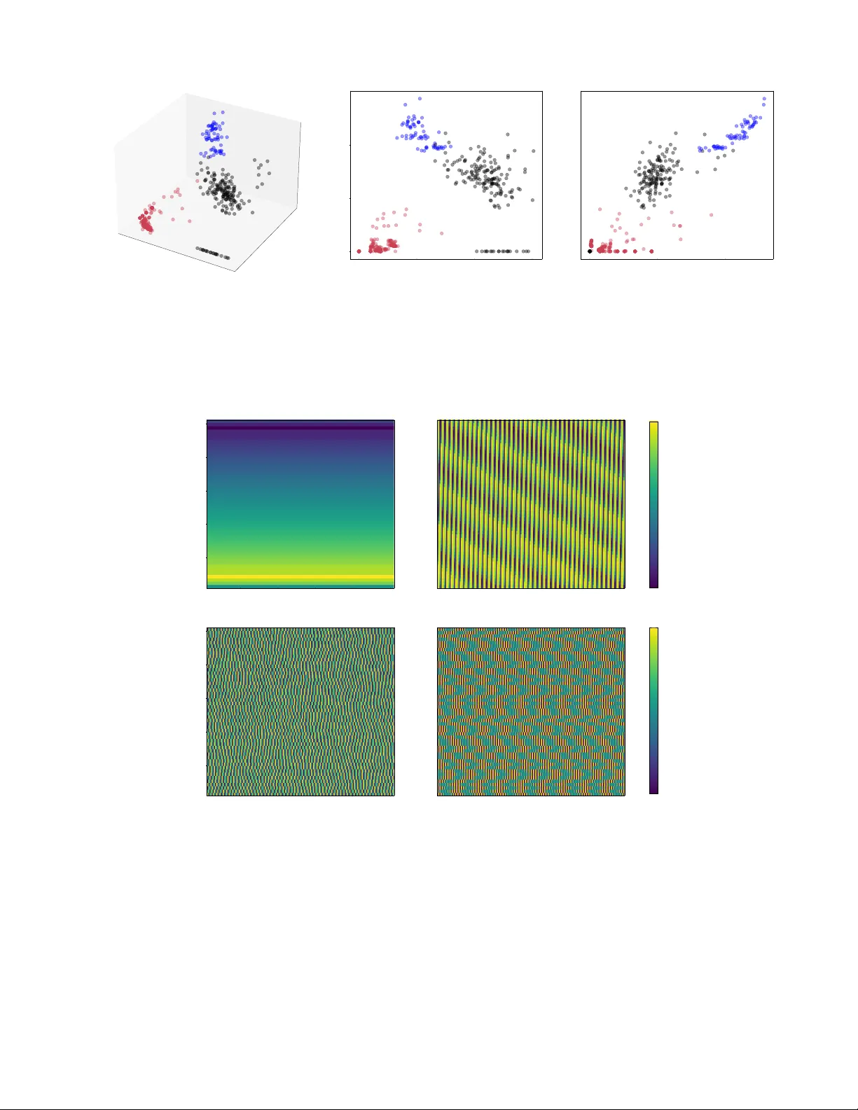
A robust metho d for classification of c himera states S. Nirmala Jenifer, 1, 2 , ∗ Riccardo Muolo, 3, 4 P aulsamy Muruganandam, 1, 5 and Timoteo Carletti 2 , † 1 Dep artment of Physics, Bhar athidasan University, Tiruchir app al li 620 024, T amil Nadu, India 2 Dep artment of Mathematics and naXys, Namur Institute for Complex Systems, University of Namur, Namur, Belgium 3 RIKEN Center for Inter disciplinary The oretic al and Mathematic al Scienc es (iTHEMS), Saitama, Jap an 4 Dep artment of Systems and Contr ol Engine ering, Institute of Scienc e T okyo (former T okyo T e ch), T okyo, Jap an 5 Dep artment of Me dic al Physics, Bhar athidasan University, Tiruchirapp al li 620 024, T amil Nadu, India Chimera states are one of the most in triguing phenomena in nonlinear dynamics, characterized b y the co existence of coheren t and incoherent b ehavior in systems of coupled iden tical oscillators. De- spite extensive studies and numerous observ ations in different settings, the developmen t of reliable and systematic metho ds to classify chimera states and distinguish them from other dynamical pat- terns remains a challenging task. Existing approac hes are often limited in scope and lac k robustness. In this w ork, we prop ose a method based on F ourier analysis com bined with statistical classification to c haracterize chimera behavior. The metho d is applied to a system of top ological signals coupled via the Dirac op erator, where it successfully captures the ric h dynamical regimes exhibited by the mo del. W e demonstrate that the prop osed approach is robust with respect to v ariations in netw ork top ology and system parameters. Beyond the specific mo del considered, the framework provides a general and automated to ol for distinguishing differen t dynamical regimes in complex systems. I. INTR ODUCTION Complex netw orks pro vide a natural framew ork for de- scribing large collections of interacting dynamical units whose collectiv e b eha vior cannot b e inferred from indi- vidual comp onen ts alone [ 1 ]. Suc h systems arise in di- v erse contexts, by including neural populations, c hemical oscillators, p o wer-grid dynamics, and ecological in terac- tions, where the interpla y b etw een in trinsic dynamics and net work structure gives rise to rich spatiotemp oral pat- terns [ 2 – 5 ]. Among these emergen t behaviors, c himera states, characterized by the coexistence of coherent and incoheren t dynamical regions within a p opulation of iden- tical oscillators, hav e attracted sustained interest due to their coun terintuitiv e nature and p otential relev ance to real-w orld phenomena. Chimera states were first rep orted by Kaneko for cou- pled maps [ 6 , 7 ], and later observed for global [ 8 – 10 ], i.e., all-to-all, and nonlo cal [ 11 – 15 ], i.e., first neighbors, couplings. How ev er, such patterns b ecame popular af- ter the studies on phase oscillators by Kuramoto and Battogtokh [ 16 ], and b y Abrams and Strogatz [ 17 ], who coined its actual name. Since then, they hav e been ob- serv ed in a wide range of mo dels and exp erimen tal sys- tems, for instance, in Josephson junction arra ys [ 18 ], electronic circuits [ 19 , 20 ], lasers [ 21 ], mec hanical oscilla- tors [ 22 ], and nano-electromechanical systems [ 23 ]. They ha ve sparked also interest b eyond the nonlinear science comm unity , since c himera-like patterns ha ve b een sug- gested as models for unihemispheric sleep observ ed in certain animals [ 24 – 26 ]. Strictly dynamically speaking, their imp ortance lies in the fact that they pro vide a con- ∗ nirmala-jenifer.selv ara j@unamur.be † timoteo.carletti@unamur.be crete example of partial sync hronization, where iden ti- cal units sub ject to identical coupling self-organize into distinct dynamical groups [ 27 – 29 ], and, now adays, sev- eral kinds of patterns ha v e b een observ ed, suc h as am- plitude chimeras [ 30 ], amplitude-mediated c himeras [ 31 ], and phase chimeras [ 32 ], to name a few. Despite their conceptual imp ortance, reliably identify- ing and characterizing c himera states remains a nontriv- ial task. A v ariety of classification metho ds hav e been prop osed, ranging from global order parameters to local coherence measures. Ho wev er, these approaches often dep end sensitively on parameter c hoices, system size, or thresholds, and may lead to ambiguous interpretations when applied to weak, transien t, or spatially irregular patterns. In practice, the distinction b et w een chimera and non-chimera regimes is not alwa ys sharply defined, and in termediate b eha viors can b e difficult to categorize in a consistent and robust wa y . Because the problem do es not hav e a definite solution yet, the developmen t of signal-based approaches that can capture gradual v aria- tions in local correlations without relying on ad ho c cri- teria, op ens new in teresting researc h av enues. In this work, we consider a system of top ological sig- nals defined on a 1 -simplicial complex, i.e., a netw ork, where dynamical v ariables are asso ciated not only with no des but also with links [ 33 ]. The mo del fits, th us, in the recen t framew ork of higher-order netw orks [ 34 – 38 ], where in teractions are not limited to pairwise connec- tions but can in v olve more complex relations enco ded by h yp ergraphs, and simplicial or cell complexes [ 39 , 40 ]. More specifically , we consider the dynamics of top ologi- cal signals coupled via the discrete Dirac op erator [ 41 ], suc h that the no des behav e as coupled oscillators, de- spite having no intrinsic oscillatory dynamics. Such set- ting has been shown to yield ric h synchronization [ 42 , 43 ] and pattern formation [ 44 – 46 ] dynamics. The adapted FitzHugh-Nagumo model [ 47 , 48 ] considered here, with 2 dynamics on b oth no des and links, exhibits a rich range of b eha viors, by including c himera, coheren t and incoherent regimes, making it a suitable b enchmark for classification tasks. Note that, while chimera states hav e b een found on hypergraphs [ 49 – 56 ], such behavior had not b een ob- serv ed in systems of coupled top ological signals. Motiv ated b y this researc h question, we develop a F ourier transform-based framework to analyze the time series, i.e., the time evolution of node signals; by start- ing from simulated data, we extract instan taneous am- plitude, phase, and frequency for the time series gener- ated from the dynamics of eac h node b y using a refined windo wed F ourier transform. W e then quantify their lo- cal v ariations across the netw ork b y computing the to- tal normalized v ariations [ 57 ], a measure of the (spatial) smo othness of the signal under study . In this wa y , we asso ciate to each time series three quan tities, the total normalized v ariation of amplitude, phase and frequency , that form the basis of a classification sc heme capable of distinguishing betw een sync hronized, c himera, and irreg- ular regimes. More precisely , w e lev erage on the use of hierarc hical clustering and dendrograms to cluster the data and thus automatically determine the class and the asso ciated dynamical behavior. The prop osed approac h pro vides a robust w ay to identify different dynamical pat- terns b y using directly measurable signal features, and it is applicable to a broad class of net work ed dynamical systems, b ey ond the one prop osed hereb y . The remainder of the man uscript is organized as fol- lo ws. Sec. I I introduces the theoretical mo del, the gov- erning equations of the system, and shows the existence of the homogeneous solutions along with their stability analysis. Sec. I I I presents the main results and the clas- sification metho d. W e conclude Sec. I I I by exploring the effects of system parameters on the observed dynamical regimes. Finally , in Sec. IV we resume our main findings and discuss p ossible future researc h directions. I I. THE MODEL W e consider a ring comp osed b y n nonlocally cou- pled identical FitzHugh-Nagumo oscillators (FHN) [ 47 , 48 , 58 ], eac h one described b y tw o dynamical v ariables, the membrane p oten tial, u i , and the rec o v ery v ariable, v j . This mo del has been prop osed to study the dynam- ics of neurons, with neurons in teracting with synaptic v ariables and vice-v ersa [ 59 ]. In this work, w e assume the membrane p otential to be anc hored to eac h node, while the recov ery v ariable is asso ciated to each link; let us observe that a similar mo del has b een prop osed in [ 43 ]. This assumption naturally sets our model in the framework of top ological signals defined on simplicial complexes, where, i.e., a no de is a 0 -simplex and a link a 1 -simplex. Moreov er, simplices of differen t dimensions are coupled through the Dirac operator [ 41 , 44 ]. Our sys- tem naturally includes simplices up to dimension 1 , hence in volving only pairwise interactions. It can, how ever, b e extended to higher-dimensional simplicial complexes to represen t higher-order, non-pairwise in teractions such as three-b ody or four-b o dy in teractions [ 34 , 35 ], as well as on cell-complexes [ 60 , 61 ]. Based on the ab o v e, the equations ruling the system ev olution, comprising no de and link dynamics coupled b y the Dirac op erator [ 41 , 44 ], are given by a du i dt = u i − u 3 i 3 − ( B 1 v ) i , (1) dv j dt = b + cv j + ( B ⊤ 1 u ) j , (2) where B 1 is the incidence matrix [ 62 ] of size n × m for a system with n no des and m links. Because each no de is connected to P neigh b ors on ei- ther side, the resulting node degree is k i = 2 P , for all i = 1 , . . . , n . The incidence matrix B 1 can thus be com- puted as follows: given an oriented link j = [ i, k ] , then B 1 [ i, j ] =      1 , k − i ≥ n − P , − 1 , k − i < n − P , 0 , otherwise . (3) Finally , let us observ e that the num b er of incoming and outgoing links of each no de is the same; w e refer to this configuration as orientation 1 (see left panel of Fig. 1 for an example with n = 8 and P = 3 ). The parameter b in Eq. ( 2 ) determines whether no des exhibit oscillatory , | b | < 1 , or excitable b ehavior, | b | > 1 [ 63 ]. Because the matrix B 1 satisfies B 1 (1 , . . . , 1) ⊤ = 0 , one can pro ve the existence of three homogeneous equi- libria ( u i , v j ) = ( √ 3 , − b/c ) , ( u i , v j ) = ( − √ 3 , − b/c ) and ( u i , v j ) = (0 , − b/c ) , the first tw o are stable while the latter is unstable. Because in the following we will b e in terested in studying a ring structure with different ori- en tations with resp ect to the one giv en by ( 3 ), we ob- serv e that, when b = 0 , the system is in v arian t under the transformations ( u, v ) → ( − u, − v ) and, thus, the dynam- ics will not dep end on the c hosen orien tation. How ev er, this inv ariance is broken when b  = 0 . F or the following analysis, w e fix b = 0 . 5 and a = 0 . 05 . The condition c < 0 ensures that recov ery v ariables deca y when w e si- lence the interactions of the latter with neurons, we thus fix c = − 0 . 01 . Let us rewrite Eqs. ( 1 ) and ( 2 ) as du i dt = a ′ ( u i − u 3 i 3 ) − a ′ X l B 1 [ i, l ] v l dv j dt = X i B 1 [ i, j ] u i + b + cv j where a ′ = 1 /a . T o determine the stability of the ho- mogeneous solution ( u i , v j ) = ( u ∗ , v ∗ ) , where ( u ∗ , v ∗ ) = ( ± √ 3 , − b/c ) or ( u ∗ , v ∗ ) = (0 , − b/c ) , w e consider the p er- turbations, δ u i = u i − u ∗ and δ v j = v j − v ∗ , w e insert them into the ab o ve equations and then we linearize to 3 1 2 3 4 5 6 7 8 1 2 3 4 5 6 7 8 1 2 3 4 5 6 7 8 FIG. 1. Sc hematic illustration of orien tation 1 , for the case n = 8 and P = 3 . In the left panel, we report the original ring, where each one of the eight no des is connected to P = 3 neigh b ors on either side. The middle panel refers to the case where Q = 1 links incident to no de 1 , hav e b een reoriented (drawn in red). In the right panel, w e sho w the case Q = P = 3 , where again we fixed no de 1 as reference (red links are the reoriented ones). get dδ u i dt = a ′ (1 − ( u ∗ ) 2 ) δ u i − a ′ X l B 1 [ i, l ] δ v l (4) dδ v j dt = X i B 1 [ i, j ] δ u i + cδ v j , (5) or in matrix form d dt  δ u δ v  = J  δ u δ v  , where we in tro duced the ( n + m ) × ( n + m ) Jacobian matrix J =  a ′ (1 − ( u ∗ ) 2 ) I n − a ′ B 1 B ⊤ 1 c I m  and the stack vec- tors δ u = ( δ u 1 , . . . , δ u n ) ⊤ and δ v = ( δ v 1 , . . . , δ v m ) ⊤ . T o gain some analytical insight into the problem, let us re- duce the dimension of the latter b y using B 1 B ⊤ 1 = L 0 , i.e., the netw ork Laplace matrix, and B ⊤ 1 B 1 = L 1 , the 1 -Ho dge-Laplace matrix. The eigen v alues of L 0 and L 1 are Λ ( α ) 0 = Λ ( α ) 1 and they can b e expressed as the square of the singular v alue b α of the matrix B 1 , namely Λ ( α ) 0 = Λ ( α ) 1 = b 2 α . On the other hand the eigenv ectors ψ α 0 and ψ α 1 ob ey B 1 ψ 1 α = b α ψ 0 α (6) B ⊤ 1 ψ 0 α = b α ψ 1 α . (7) W e can no w pro ject δ u i and δ v j on to the eigen basis: δ u i = P α δ ˆ u α ( ψ 0 α ) i and δ v j = P α δ ˆ v α ( ψ 1 α ) j . By using Eqs. ( 6 ) and ( 7 ) we then get from Eqs. ( 4 ) and ( 5 ) dδ ˆ u α dt = a ′ (1 − ( u ∗ ) 2 ) δ ˆ u α − a ′ b α δ ˆ v α dδ ˆ v α dt = cδ ˆ v α + b α δ ˆ u α or in matrix form d dt  δ ˆ u α δ ˆ v α  =  a ′ (1 − ( u ∗ ) 2 ) − a ′ b α b α c   δ ˆ u α δ ˆ v α  =: J α  δ ˆ u α δ ˆ v α  The stability of the homogeneous solution ( u ∗ , v ∗ ) can b e determined by studying the sp ectrum of J α . A straigh t- forw ard computation returns the roots of the c haracter- istic p olynomial λ = a ′ u ′ + c ± p ( a ′ u ′ + c ) 2 − 4( ca ′ u ′ + a ′ b 2 α ) 2 , where u ′ = (1 − ( u ∗ ) 2 ) . By direct insp ection of those ro ots, w e can thus conclude that the fixed point ( u ∗ , v ∗ ) = (0 , − b/c ) is alw ays unstable, whereas the fixed p oin ts ( u ∗ , v ∗ ) = ( ± √ 3 , − b/c ) are alw a ys stable, and this holds true for an y P . T o determine the domain of stability of the homoge- neous solution, ( u i , v j ) = ( √ 3 , − b/c ) , we p erformed n u- merical simulations to determine the fraction, f , of initial conditions starting inside a ball of radius R , centered at the equilibrium, whose orbits remain in the same ball after a giv en interv al of time. W e are in particular inter- ested in the dependence of f on P for a fixed netw ork size. More precisely w e fixed n = 100 and for P ranging in [1 , 30] , w e considered 50 v alues of R in the in terv al [0 . 01 , 1 . 5] . F or every radius, the simulation w as rep eated N = 20 times with differen t initial conditions. Let N ′ denote the num ber of realizations for which the solution remains within the prescrib ed radius R , we then compute the ratio f = N ′ / N . When N ′ / N = 1 , the equilibrium is stable for all realizations and it is therefore classified as stable. As the radius increases, N ′ decreases, indicating the onset of instability (see Fig. 2 ). The existence of the homogeneous solution, where all u i con verge to √ 3 and v j to − b/c and its relativ ely large attraction basin, impedes the emergence of c himera states as well as other spatially heterogeneous solutions. F or this reason, we decided to modify the links orienta- tion and determine conditions to ensure the emergence of those states. Th us, starting from the oriented ring with a given num b er of nearest neighbors for each no de, 2 P , evenly distributed on the left and on the right, w e 4 10 20 30 P 0 . 3 0 . 6 0 . 9 1 . 2 1 . 5 Sphere radius ( R ) 0 . 0 0 . 2 0 . 4 0 . 6 0 . 8 1 . 0 N 0 / N FIG. 2. Stability domain of the homogeneous solution u i = √ 3 , v j = − b/c for the FHN model defined on a ring of n = 100 no des with a v ariable n um b er of links con trolled by the parameter P . The fraction f = N ′ / N of initial conditions, starting within a ball of radius R and remaining in the same ball after a sufficiently long time (i.e., sta ying “close” to the starting p oin t), is shown as a function of P . A nonmonotonic b eha vior is observ ed: for small P , nearly 100% of the orbits remain within a ball of radius R ∼ 0 . 6 . F or larger P , the stability domain expands, with f = 1 up to R ∼ 1 at P = 20 . F or ev en larger v alues of P , the stabilit y domain slowly decreases. in verted the orientation of Q ∈ { 1 , . . . , P } links (see mid- dle panel of Fig. 1 for the case Q = 1 and the righ t panel where we sho w the case Q = 3 , in b oth cases P = 3 ). Because of the inv ariance by rotation, all the nodes are equiv alent, before to reorient the links, and thus we de- cided to fo cus on node 1 . Let us observ e that now the homogeneous state is no longer a solution: indeed, the underlying structure does not exhibit anymore a rotation in v ariance. Before to pro ceed with the presentation of the numer- ical results, let us observe that w e can define a different orien tation strategy , where again the homogeneous state cannot be a solution. The latter structure is defined b y using the incidence matrix B 1 [ i, j ] =      1 , i > k , − 1 , i < k , 0 , otherwise , (8) b eing j = [ i, k ] the oriented link according to the no de index. W e refer to this case as orientation 2 . The inter- ested reader can find a definition of this orien tation in App endix D and an example of a ring with n = 8 nodes and P = 3 is shown in Fig. 17 . By an ticipating on the follo wing, we will sho w that this second structure will be more robust with resp ect to the emergence of c himera state, once we randomly reorien t links (see Appendix D ). I II. METHOD AND RESUL TS The aim of this section is to introduce and discuss the metho d used to classify the dynamical b ehav iors exhib- ited b y the FHN system and the numerical results ab out the p ossible dynamical states exhibited by system ( 1 )- ( 2 ) defined on the ring with orientation 1 . W e first present our analysis in the case where we reorien t the maxim um allo wed num ber of links, i.e., Q = P , still fo cusing on no de 1 , and we let P to v ary from 1 to n/ 2 − 1 , b eing n an even integer. Then w e will show the remaining case where also Q v aries in { 0 , . . . , P } . This analysis will b e presen ted for a fixed set of mo del parameters, a , b and c , their impact will b e shortly studied next. Based on some preliminary study , we observ e that the system exhibits an oscillatory b eha vior, that c an b e reg- ular or irregular, b oth in time and in space. In Fig. 3 , we rep ort three typical cases for a ring of n = 50 no des and parameters a = 0 . 05 , b = 0 . 5 and c = − 0 . 01 ; in panel (a) w e can observ e a regular state in whic h the system b eha v es as a trav eling wa v e ( Q = P = 9 ), in panel (b) w e displa y a chimera state where regular oscillations co exist with irregular behavior ( Q = P = 12 ), in panel (c) we sho w a disordered state where, i.e., no regular oscillations can b e detected ( Q = P = 21 ). T o numerically integrate the equations of motion w e set initial conditions δ -close to ( u ∗ , v ∗ ) = (0 , 0) and we then use the tsit5 solv er (5th order adaptiv e step size Runge Kutta method [ 64 ]) to ob- tain time series in the time in terv al [0 , 1000] , ev ery 0 . 01 time units. More precisely , w e set δ = 0 . 001 and w e draw uniform random n um b ers ∆ u i ∈ U [ − 1 , 1] and, similarly , for ∆ v j , to even tually set u i (0) = u ∗ + δ ∆ u i i = 1 , . . . , n v j (0) = v ∗ + δ ∆ v j j = 1 , . . . , m . T o quan tify these dynamics, w e prop ose a metho d ro oted on the extraction of information ab out the instantaneous phases, amplitudes and frequencies from the time series obtained by numerically solving the dynamical equations. The metho d is based on an adapted use of F ourier anal- ysis and consists, roughly , in associating to each no de a v alue for the oscillation amplitude, ⟨ a i ⟩ , the oscillation frequency , ⟨ Ω i ⟩ , and its constan t phase, ⟨ θ i ⟩ (see Ap- p endix A for a complete description and Fig. 4 where w e presen t the latter quan tities asso ciated to the dynamical b eha viors shown in Fig. 3 ). Even tually , to measure the spatial dep endence of those quan tities, we define the to- tal (normalized) v ariation [ 57 ] for phases, amplitudes and frequencies. The total normalized v ariation is a measure of the lo cal regularity of those quantities computed by 5 960 970 980 990 1000 t 10 20 30 40 50 nodes 960 970 980 990 1000 t 10 20 30 40 50 960 970 980 990 1000 t 10 20 30 40 50 (a) (b) (c) ° 2 0 2 u ( t ) FIG. 3. Typical dynamical b ehaviors . Numerical sim ulations of mo del ( 1 ) and ( 2 ) in orientation 1 , illustrating three distinct dynamical regimes: ordered behavior (panel (a), Q = P = 9 ), a chimera state (panel (b), Q = P = 12 ), and a disordered state (panel (c), Q = P = 21 ). The remaining parameters are n = 50 , a = 0 . 05 , b = 0 . 5 , and c = − 0 . 01 . Simulations are p erformed using the T sit5 solver o ver the time interv al [0 , 1000] . F or clarity , only the ev olution of u i ( t ) ov er the final time windo w t ∈ [950 , 1000] is shown. considering differences among nearby p oin ts: V θ = 1 π n n X i =1 min { v θ i , 2 π − v θ i } (9) V a = 1 n n X i =1 |⟨ a ⟩ i +1 − ⟨ a ⟩ i | (10) V Ω = 1 n n X i =1 |⟨ Ω ⟩ i +1 − ⟨ Ω ⟩ i | , (11) with v θ i = |⟨ θ ⟩ i +1 − ⟨ θ ⟩ i | . Let us also observe that indexes should be considered modulo n , i.e., n + 1 ≡ 1 , b ecause of the ring structure. The smaller the v ariation, the smoother the signal and vice v ersa. Hence, the latter qualifies to b e a useful metric to classify chimera patterns. Let us consider the results presen ted in Fig. 4 . Panels in the column (a) show a v ery regular b eha vior for the v ariations: the frequency is constant, the amplitude slo wly oscillated in space, fi- nally the phases clearly shown a linear dep endence on the no de p osition. W e are th us facing to a wa v e whose amplitude is not constan t across the ring. This b ehav- ior can thus b e classified as regular one. The panels in the column (b) displa y a differen t behavior: some no des sho w a constant frequency while other one a “parabola– lik e” dep endence on the no de index, this is the classical b eha vior observ ed for chimera states [ 16 , 17 , 65 ]. The amplitudes also exhibit a nontrivial but smo oth dep en- dence on the node index, whereas the phases b ehav e in a more irregular wa y . Finally , panels in the column (c) displa y an irregular b eha vior in the three quantities, even if small in amplitude and frequency . By applying the prop osed metho d to compute the v ariations of data shown in Fig. 4 w e obtain the fol- lo wing v alues for ( V θ , V a , V Ω ) : (0 . 0683 , 0 . 082 , 0 . 0022) in the case of ordered b eha vior (column (a)), (0 . 2301 , 0 . 1110 , 0 . 1087) for the chimera state (column (b)) and (0 . 4554 , 0 . 04452 , 0 . 0478) for the disordered case (column (c)). Ev en if a clear trend is shown, with higher v ariations associated to more irregular b eha vior as al- ready stated, it also app ears that there is not a clear “uni- v ersal” threshold allowing to separate the differen t cases. F or this reason, we resort to a classification algorithm to extract hidden patterns in the data. More precisely , w e compute ( V θ , V a , V Ω ) for all Q = P in { 2 , . . . , 24 } and for eac h P w e rep eat 20 times the sim ulation. W e thus obtain a database comp osed by 460 triplets ( V θ , V a , V Ω ) , that w e pre-pro cess b y rescaling in [0 , 1] by using the Python function MinMaxsc aler . The use of the agglomerative clustering algorithm [ 66 ], i.e., a w ell known hierarc hical clustering algorithm, allows us to construct a dendrogram of the giv en data (see panel (a) of Fig. 5 ). F or the c ho- sen v alue of the depth thr eshold , d , w e observ e three, well separated, classes that, interestingly enough, corresp ond to the three typical b eha viors ab ov e emphasized: regular, c himera and irregular states. In the panel (b) of Fig. 5 , w e present a 2 D pro jection of the 3 D database, where we used only the coordinates ( V θ , V a ) ; let us observe that w e here used to original v alues for the v ariations, i.e., prior to the pre-processing. Three clusters are clearly visible; the red cluster (class 1) corresp onds to the ordered states asso ciated to smaller v ariations, the blue cluster (class 2) corresp ond to c himeras, showing larger v ariations in am- plitudes and medium v ariation in phases, the black clus- ter (class 3) corresp onds to the disordered states, with larger v ariation in phases and medium v ariation in am- plitude. In Fig. 15 we will present a complete 3 D view of the data (panel (a)) together with the pro jections on the planes ( V θ , V Ω ) (panel (b)) and ( V a , V Ω ) (panel (c)). With this pro jection, but also in the construction of the dendogram, we lose information ab out the used v alue of Q = P . Hence, for each v alue of Q = P ∈ { 2 , . . . , 24 } , w e computed the statistical mo de to identify the most frequen t class among the 20 realizations. Let us observe that this step is necessary b ecause, for some v alues of 6 10 20 30 40 50 ° 3 ° 2 ° 1 0 1 2 3 10 20 30 40 50 ° 3 ° 2 ° 1 0 1 2 3 10 20 30 40 50 ° 3 ° 2 ° 1 0 1 2 3 (a1) (b1) (c1) AAAB/nicbVBNSwMxEM36WetXVTx5CRbBU9kVqR6LXjxWsB/QXUo2nbah2eySzAplKfhXvHhQxKu/w5v/xrTdg7Y+GHh5b4bMvDCRwqDrfjsrq2vrG5uFreL2zu7efungsGniVHNo8FjGuh0yA1IoaKBACe1EA4tCCa1wdDv1W4+gjYjVA44TCCI2UKIvOEMrdUvHvmRqIIH6OARkvp69uqWyW3FnoMvEy0mZ5Kh3S19+L+ZpBAq5ZMZ0PDfBIGMaBZcwKfqpgYTxERtAx1LFIjBBNlt/Qs+s0qP9WNtSSGfq74mMRcaMo9B2RgyHZtGbiv95nRT710EmVJIiKD7/qJ9KijGdZkF7QgNHObaEcS3srpQPmWYcbWJFG4K3ePIyaV5UvGqlen9Zrt3kcRTICTkl58QjV6RG7kidNAgnGXkmr+TNeXJenHfnY9664uQzR+QPnM8fU0aVvg== → ω ↑ 10 20 30 40 50 1 2 3 10 20 30 40 50 1 2 3 10 20 30 40 50 1 2 3 (a2) (b2) (c2) AAAB+XicbZDLSsNAFIZP6q3WW9Slm8EiuCqJSHVZdOOygr1AE8pketoOnUzCzKRQQt/EjQtF3Pom7nwbp5eFtv4w8PGfczhn/igVXBvP+3YKG5tb2zvF3dLe/sHhkXt80tRJphg2WCIS1Y6oRsElNgw3AtupQhpHAlvR6H5Wb41RaZ7IJzNJMYzpQPI+Z9RYq+u6gaByIJDQQM2h65a9ijcXWQd/CWVYqt51v4JewrIYpWGCat3xvdSEOVWGM4HTUpBpTCkb0QF2LEoaow7z+eVTcmGdHuknyj5pyNz9PZHTWOtJHNnOmJqhXq3NzP9qncz0b8OcyzQzKNliUT8TxCRkFgPpcYXMiIkFyhS3txI2pIoyY8Mq2RD81S+vQ/Oq4lcr1cfrcu1uGUcRzuAcLsGHG6jBA9ShAQzG8Ayv8Obkzovz7nwsWgvOcuYU/sj5/AFUWZN7 → a ↑ 10 20 30 40 50 1 2 3 4 10 20 30 40 50 1 2 3 4 10 20 30 40 50 1 2 3 4 (a3) (b3) (c3) AAAB/nicbVDLSsNAFJ3UV62vqLhyM1gEVyURqS6LbtxZwT6gCWUyvWmHTiZhZiKUUPBX3LhQxK3f4c6/cZpmoa0HLpw5517m3hMknCntON9WaWV1bX2jvFnZ2t7Z3bP3D9oqTiWFFo15LLsBUcCZgJZmmkM3kUCigEMnGN/M/M4jSMVi8aAnCfgRGQoWMkq0kfr2kceJGHLA3l0EQ+LJ/NW3q07NyYGXiVuQKirQ7Ntf3iCmaQRCU06U6rlOov2MSM0oh2nFSxUkhI7JEHqGChKB8rN8/Sk+NcoAh7E0JTTO1d8TGYmUmkSB6YyIHqlFbyb+5/VSHV75GRNJqkHQ+UdhyrGO8SwLPGASqOYTQwiVzOyK6YhIQrVJrGJCcBdPXibt85pbr9XvL6qN6yKOMjpGJ+gMuegSNdAtaqIWoihDz+gVvVlP1ov1bn3MW0tWMXOI/sD6/AENRZWR → ! ↑ AAAB7HicbVBNS8NAEJ3Ur1q/qh69BIvgqSQi1WPRi8cKpi20oWw2k3bpZjfsboRS+hu8eFDEqz/Im//GbZuDVh8MPN6bYWZelHGmjed9OaW19Y3NrfJ2ZWd3b/+genjU1jJXFAMquVTdiGjkTGBgmOHYzRSSNOLYica3c7/ziEozKR7MJMMwJUPBEkaJsVIgZIx6UK15dW8B9y/xC1KDAq1B9bMfS5qnKAzlROue72UmnBJlGOU4q/RzjRmhYzLEnqWCpKjD6eLYmXtmldhNpLIljLtQf05MSar1JI1sZ0rMSK96c/E/r5eb5DqcMpHlBgVdLkpy7hrpzj93Y6aQGj6xhFDF7K0uHRFFqLH5VGwI/urLf0n7ou436o37y1rzpoijDCdwCufgwxU04Q5aEAAFBk/wAq+OcJ6dN+d92Vpyiplj+AXn4xv5yo7Q nodes AAAB7HicbVBNS8NAEJ3Ur1q/qh69BIvgqSQi1WPRi8cKpi20oWw2k3bpZjfsboRS+hu8eFDEqz/Im//GbZuDVh8MPN6bYWZelHGmjed9OaW19Y3NrfJ2ZWd3b/+genjU1jJXFAMquVTdiGjkTGBgmOHYzRSSNOLYica3c7/ziEozKR7MJMMwJUPBEkaJsVIgZIx6UK15dW8B9y/xC1KDAq1B9bMfS5qnKAzlROue72UmnBJlGOU4q/RzjRmhYzLEnqWCpKjD6eLYmXtmldhNpLIljLtQf05MSar1JI1sZ0rMSK96c/E/r5eb5DqcMpHlBgVdLkpy7hrpzj93Y6aQGj6xhFDF7K0uHRFFqLH5VGwI/urLf0n7ou436o37y1rzpoijDCdwCufgwxU04Q5aEAAFBk/wAq+OcJ6dN+d92Vpyiplj+AXn4xv5yo7Q nodes AAAB7HicbVBNS8NAEJ3Ur1q/qh69BIvgqSQi1WPRi8cKpi20oWw2k3bpZjfsboRS+hu8eFDEqz/Im//GbZuDVh8MPN6bYWZelHGmjed9OaW19Y3NrfJ2ZWd3b/+genjU1jJXFAMquVTdiGjkTGBgmOHYzRSSNOLYica3c7/ziEozKR7MJMMwJUPBEkaJsVIgZIx6UK15dW8B9y/xC1KDAq1B9bMfS5qnKAzlROue72UmnBJlGOU4q/RzjRmhYzLEnqWCpKjD6eLYmXtmldhNpLIljLtQf05MSar1JI1sZ0rMSK96c/E/r5eb5DqcMpHlBgVdLkpy7hrpzj93Y6aQGj6xhFDF7K0uHRFFqLH5VGwI/urLf0n7ou436o37y1rzpoijDCdwCufgwxU04Q5aEAAFBk/wAq+OcJ6dN+d92Vpyiplj+AXn4xv5yo7Q nodes FIG. 4. F ourier indicators . A v erage phases ⟨ θ ⟩ (top ro w), a v erage amplitudes ⟨ a ⟩ (middle row), and av erage frequencies ⟨ Ω ⟩ (bottom row) obtained from the time series shown in Fig. 3 for P = 9 , P = 12 , and P = 21 . Column (a) corresponds to ordered b eha vior, showing a smooth dep endence of all three quantities on the no de index. Column (b) displays a c himera state, c haracterized by the typical distribution of frequencies; here, the av erage amplitudes remain smo oth, while the phases exhibit less regularity . Column (c) shows a disordered state, mark ed b y small but irregular v ariations in b oth amplitude and frequency , and highly irregular phase b ehavior. The corresp onding v ariation v alues ( V θ , V a , V Ω ) are (0 . 0683 , 0 . 082 , 0 . 0022) for the ordered state in column (a), (0 . 2301 , 0 . 1110 , 0 . 1087) for the chimera state in column (b), and (0 . 4554 , 0 . 04452 , 0 . 0478) for the disordered state in column (c). Q = P , different dynamical b eha viors can b e observed. The results are rep orted in the panel (c) of Fig. 5 and w e can obv erse the presence of ordered states for Q = P ranging from 2 to 10 , c himera states for the Q = P ∈ { 11 , 12 , 13 } , and then disordered states for larger v alues of Q = P , but for the v alues { 16 , 17 , 18 } asso ciated to regular b eha vior. Let us note that by lo wering the depth threshold, the dendrogram first iden tifies four classes and then fiv e (see, Fig. 12 and Fig. 13 , resp ectiv ely). It is w orth mention- ing that, in the former case, the irregular class splits into t wo new classes, while, in the latter case, the regular class also splits in to tw o classes. How ev er, in all the cases, the c himera class main tains its “in tegrit y”. It is w orth men- tion here that other clustering algorithms could b e used based on the “shap e” of the av ailable data, for instance if 7 0 2 4 6 8 10 12 d 0 . 0 0 . 2 0 . 4 0 . 6 V µ 0 . 00 0 . 05 0 . 10 V a 4 8 12 16 20 24 P 3 1 2 C lasses (a) (b) (c) FIG. 5. Classification of dynamical behaviors by using the v ariations V θ , V a and V Ω , in the case of orien tation 1 and Q = P links ha v e b een reoriented. In panel (a) we rep ort the dendrogram obtained from the hierarchical clustering by using the v alues of ( V θ , V a , V Ω ) . Branch lengths represent in ter-cluster distances prior to merging, indicating tw o well-separated groups. The horizon tal black line denotes the depth threshold used to determine the num b er of classes. In panel (b) we rep ort the pro jection in the plane ( V θ , V a ) of the three obtained clusters b y using the agglomerativ e clustering: the red cluster (class 1) corresp onds to the ordered states, the blue cluster (class 2) corresp ond to chimeras, and the blac k cluster (class 3) corresp onds to the disordered states. Panel (c) sho ws an alternativ e view of the classification as a function of P = Q in the range { 2 , . . . , 24 } ; to each v alue of P = Q we asso ciate the dominant class, i.e., determined from the statistical mo dal cluster mem b ership of ( V θ , V a , V Ω ) and we can obv erse the presence of ordered states for Q = P ranging from 2 to 10 , chimera states for the Q = P ∈ { 11 , 12 , 13 } , and then disordered states for larger v alues of Q = P , but for the v alues { 16 , 17 , 18 } . a preliminary analysis sho ws that clusters are w ell spher- ically separated, we could use K-me ans . W e then consider the more general case where P and Q v ary separately . More precisely for each P ∈ { 3 , . . . , 24 } w e let Q ∈ { 0 , . . . , P } and for eac h couple ( P, Q ) we con- sider 20 realizations b y randomly changing initial con- ditions. By follo wing the same procedure ab o ve pre- sen ted, we gather 6380 triplets ( V θ , V a , V Ω ) and we apply the same classification algorithm. Three main classes are again found, corresp onding to ordered, c himera and dis- ordered states, see panel (a) of Fig. 6 ; in panel (b) we sho w a pro jection in the plane ( V θ , V a ) . Finally in the panel (c) we sho w, for eac h v alue of ( P , Q ) the associated class, defined again by using the statistical mo de of the 20 realizations; black points corresp ond to disordered state, blue points to chimera b eha vior and red p oints to regu- lars one. In addition to the P v alues for whic h we found c himera in the case P = Q , we here observe c himera also for P = 10 and Q = 4 , 5 , 6 , 7 . The results presen ted so far ha v e b een obtained for a fixed set of model parameters, a = 0 . 05 , b = 0 . 5 and c = − 0 . 01 , our aim is to no w briefly study the effects of those parameters on the dynamics. W e thus fix again a ring made of n = 50 nodes, and select three v alues of P (w e are here considering the case Q = P ), each one cor- resp onding to a main dynamical b eha vior, i.e., regular ( P = 6 ), chimera ( P = 12 ) and irregular ( P = 21 ), for the ab ov e fixed v alues of a , b and c . W e then v ary a and b and we determine the system outcome; let us observe that to realize this last step we used the classification metho d described ab o ve. More precisely , for some v alues of b ∈ [0 . 6 , 1 . 5] , we n umerically determine the time evo- lution of u i ( t ) and v j ( t ) , we apply the F ourier method to compute ⟨ a i ⟩ , ⟨ Ω i ⟩ and ⟨ θ i ⟩ , and then we compute the normalized v ariations. Ev en tually we lo ok to whic h class the triplet ( V a , V Ω , V θ ) b elongs to, to conclude ab out the dynamical behavior. The results are rep orted in Fig. 7 where w e show, for ease of visualization, the pro jection in the ( V θ , V a ) plane where the background shows with light colors the classes obtained with fixed b = 0 . 5 . Panel (a) corresp onds to the choice P = 6 ; for each b we show the v alues of ( V θ , V a ) corresp onding to the statistical mo de computed from 10 replicas, as colored diamonds accord- ing to the v alue of b . One can observe that all the points lie in the region corresp onding to the regular b ehavior. Stated differen tly , for all v alues of b the system exhibits a regular behavior. P anel (b) displa ys the case P = 12 , b y using the same ideas w e rep ort the v alues of ( V θ , V a ) computed for each b as colored diamonds, the darker the larger the v alue of b ; all the p oin ts b elong to the class asso ciated to chimera states. Finally , panel (c) presents the case P = 21 ; the v alues of ( V θ , V a ) lie in the class asso ciated to irregular b ehavior for all b . In conclusion, w e hav e shown that b y changing b ∈ [0 . 6 , 1 . 5] the system cannot change dynamical b eha vior. W e then rep eat a similar analysis by v arying a ∈ [0 . 01 , 0 . 1] . The results are sho wn in Fig. 8 b y applying the same ideas of the previous case. In panel (a) ( P = 6 ) and panel (c) ( P = 21 ), we can observe that the couples ( V θ , V a ) , again rep orted as diamond colored according to the v alue of a , remain in the same class, i.e., the system exhibits the same behavior. A new phenomenon is visi- ble in panel (b)( P = 12 ): w e can now observ e that points are spread among tw o classes, the regular one for small 8 0 10 20 30 d 0 . 0 0 . 2 0 . 4 0 . 6 V µ 0 . 00 0 . 05 0 . 10 V a 4 8 12 16 20 24 P 0 4 8 12 16 20 24 Q (a) (b) (c) FIG. 6. Classification of dynamical behaviors by using the v ariations V θ , V a and V Ω , in the case of orien tation 1 and P , Q links ha v e b een reorien ted with 0 ≤ Q ≤ P . In panel (a) we sho w the dendrogram obtained from hierarc hical clustering of ( V θ , V a , V Ω ) ; branc h lengths represent inter-cluster distances prior to merging, indicating t wo well-separated groups. P anel (b) displa ys a 2 D pro jection in the plane V θ , V a of the clusters so far obtained; p oints hav e b een colored according to their class: class 1 (red) asso ciated to the ordered states, class 2 (blue) to denote chimeras and class 3 (black) corresp onds to the disordered states. In panel (c) w e rep ort the classification as a function of P and Q . F or eac h v alue of the latter the dominan t class i s determined from the mo dal cluster membership of ( V θ , V a , V Ω ) . 0 . 0 0 . 2 0 . 4 0 . 6 V µ 0 . 00 0 . 05 0 . 10 0 . 00 V a 0 . 0 0 . 2 0 . 4 0 . 6 V µ 0 . 00 0 . 05 0 . 10 0 . 0 0 . 2 0 . 4 0 . 6 V µ 0 . 00 0 . 05 0 . 10 (a) (b) (c) 0 . 6 0 . 8 1 . 0 1 . 2 1 . 4 b FIG. 7. Impact of the parameter b on system dynamics . F or v alues of the parameter b in [0 . 6 , 1 . 5] w e compute the normalized total v ariations associated to the F ourier metrics for the orbits. W e then rep ort the v alues ( V θ , V a ) as diamonds in the plane ( V θ , V a ) containing in bac kground also the classes obtained so far with fixed b = 0 . 5 . Diamonds are colored according to the v alue of b , the larger the v alue the darker the color. P anel (a) corresponds to Q = P = 6 , we can observe that all the v alues of ( V θ , V a ) lie in the same class, that corresp onds to regular behavior. P anel (b) sho ws the case Q = P = 12 , here again the diamonds all remain in the class asso ciated to chimera states. Panel (c) displays the case Q = P = 21 , one more time the p oin ts b elong to a single class, the irregular one. v alues of a , i.e., lighter color, and the chimera one for larger v alues of a , i.e., dark er color. The transition v alue b eing ab out a ∼ 0 . 03 . In this Section, we ha ve in tro duced and discussed a classification metho d capable to cle arly discriminate b e- t ween regular, irregular and chimera state, allo wing thus to answ er to the c hallenging question on the existence of a threshold v alue used with the v arious chimera indi- cators a v ailable in the literature. The proposed metho d can b e summ arized in the following pip eline: 1. T o create time series from n umerical simulations or obtain them from exp erimen ts; 2. T o p erform the (mo dified) F ourier analysis to ex- tract relev ant information ab out phases, ampli- tudes and frequency; 3. T o compute the (normalized) total v ariations to compact the information obtained from the previ- ous p oin t; 4. T o apply a statistical classification sc heme to ex- tract the dynamical features from the data. Let us observ e that the prop osed sc heme goes beyond the presen t application on chimera states, b oth in terms of used mo del and researc h question. Let us also stress that the strength of the metho d relies on the se quence 9 0 . 0 0 . 2 0 . 4 0 . 6 V µ 0 . 00 0 . 05 0 . 10 V a 0 . 0 0 . 2 0 . 4 0 . 6 V µ 0 . 00 0 . 05 0 . 10 0 . 0 0 . 2 0 . 4 0 . 6 V µ 0 . 00 0 . 05 0 . 10 (a) (b) (c) 2 4 6 8 10 a £ 10 ° 2 FIG. 8. Impact of the parameter a on system dynamics . F or v alues of the parameter a in [0 . 01 , 0 . 1] we compute the normalized total v ariations associated to the F ourier metrics for the orbits. W e then rep ort the v alues ( V θ , V a ) as diamonds in the plane ( V θ , V a ) containing in bac kground also the classes obtained so far with fixed a = 0 . 05 . Diamonds are colored according to the v alue of a , the larger the v alue the darker the color. P anel (a) corresp onds to Q = P = 6 , w e can observ e that all the v alues of ( V θ , V a ) lie in the same class, that corresp onds to regular b eha vior. Panel (b) sho ws the case Q = P = 12 . Here, ligh t diamonds, i.e., associated to small v alues of a , remain in the regular class, while dark er diamonds, i.e., for larger v alues of a , fall in the c himera states. Panel (c) displa ys the case Q = P = 21 ; one more time the p oints b elong to a single class, the irregular one. of steps. Ho w ever, each steps can b e realized with large freedom, i.e., one can use any n umerical sc heme to in te- grate the system or use data gathered from exp eriments. One can use other metho ds to extract information about the oscillating behavior of the orbit, suc h as w av elets, and, finally , also for the classification step, one can re- sort to other metho ds, c hosen according to a preliminary analysis of data distribution. IV. CONCLUSION In this work, we in tro duced a method to classify c himera states based on signal features extracted from time series. Starting from the simulated dynamics, i.e., the time series of each node, we computed instantaneous phases, amplitudes, and frequencies via the a mo dified F ourier method, relying on the use of windo wed data. Then, w e ev aluated their total normalized v ariations to obtain a measure of local regularity of the computed quan tities. These indicators yield a compact represen- tation of the spatial organization of the system. By em- b edding the latter in a three-dimensional space and by applying hierarc hical clustering algorithms and dendro- grams, w e obtained a classification of the observed dy- namical regimes without relying on ad ho c thresholds. As an example, we considered the FitzHugh–Nagumo mo del with dynamics defined on b oth nodes and links within the framew ork of topological signals. This set- ting, provided a system with sufficien tly ric h b ehavior, by including coherent, c himera, and irregular regimes. W e analyzed t w o orien tations for the links of the 1 -simplicial complex used to couple the v ariables. W e then in ves- tigated the effects of the coupling range and the num- b er of reoriented links to generate a v ariet y of dynam- ical patterns on whic h to test the metho d. W e then tested the prop osed approach on the resulting time se- ries and sho wed that it was able to distinguish betw een ordered, chimera, and disordered states. In particular, the metho d captured intermediate and w eakly structured regimes that are usually difficult to identify by using stan- dard measures. The classification remained stable across differen t parameter v alues and net w ork configurations, indicating that the pro cedure is robust. Finally , since the metho d relies only on signal-based quan tities and not on specific prop erties of the underly- ing mo del, it is not restricted to the framework consid- ered here, but can b e directly applied to other dynamical systems, as well as to exp erimen tal or real-w orld data, whenev er a systematic identification of different dynam- ical regimes is required. A CKNOWLEDGMENTS The work of S.N.J. is supp orted by the Institutional call for do ctoral fellowship (CER UNA), Universit y of Na- m ur. R.M. ac knowledges JSPS KAKENHI 24KF0211 for financial support. The w ork of P .M. is supp orted by the Ministry of Education-Rashtriy a Uc hchatar Shiksha Abhiy an (MoE R USA 2.0): Bharathidasan Universit y – Ph ysical Sciences. A UTHOR’S CONTRIBUTION S.N.J.: soft ware, metho dology , in vestigation, visual- ization, formal analysis, v alidation, writing – original 10 draft, writing – review and editing. R.M.: conceptu- alization, supervision, writing – original draft, writing – review and editing. P .M. sup ervision. T.C.: conceptual- ization, metho dology , inv estigation, visualization, formal analysis, supervision, writing – original draft, writing – review and editing. All authors read and appro ved the man uscript. [1] V. Latora, V. Nicosia, and G. Russo, Complex Net- works: Principles, Metho ds and Applic ations , edited b y V. Nicosia and G. Russo (Cam bridge Universit y Press, Cam bridge, 2017). [2] S. Bo ccaletti, V. Latora, Y. Moreno, M. Cha vez, and D.- U. Hwang, Complex netw orks: Structure and dynamics, Ph ys. Rep. 424 , 175 (2006) . [3] A. Arenas, A. Díaz-Guilera, J. Kurths, Y. Moreno, and C. Zhou, Synchronization in complex netw orks, Phys. Rep. 469 , 93 (2008) . [4] C. R. Laing, The dynamics of chimera states in heteroge- neous Kuramoto netw orks, Physica D 238 , 1569 (2009) . [5] J. Sawic ki, R. Berner, S. A. M. Loos, M. An v ari, R. Bader, W. Barfuss, N. Botta, N. Brede, I. F rano vić, D. J. Gauthier, et al. , P ersp ectiv es on adaptive dynami- cal systems, Chaos 33 , 071501 (2023) . [6] K. Kanek o, Period-doubling of kink-antikink patterns, quasip eriodicity in antiferro-lik e structures and spatial in termittency in coupled logistic lattice: T ow ards a pre- lude of a “field theory of chaos”, Prog. Theor. Phys. 72 , 480 (1984) . [7] K. Kanek o, Clustering, coding, switc hing, hierarchical ordering, and control in a netw ork of chaotic elements, Ph ysica D 41 , 137 (1990) . [8] V. Hakim and W.-J. Rapp el, Dynamics of the globally coupled complex Ginzburg-Landau equation, Phys. Rev. A 46 , R7347 (1992) . [9] N. Nak agaw a and Y. Kuramoto, Collective chaos in a p opulation of globally coupled oscillators, Prog. Theor. Ph ys. 89 , 313 (1993) . [10] M.-L. Chabanol, V. Hakim, and W.-J. Rapp el, Collec- tiv e chaos and noise in the globally coupled complex Ginzburg-Landau equation, Physica D 103 , 273 (1997) . [11] Y. Kuramoto, Scaling behavior of turbulent oscillators with non-lo cal in teraction, Prog. Theor. Phys. 94 , 321 (1995) . [12] Y. Kuramoto and H. Nak ao, Origin of p ow er-law spa- tial correlations in distributed oscillators and maps with nonlo cal coupling, Phys. Rev. Lett. 76 , 4352 (1996) . [13] Y. Kuramoto and H. Nak ao, Po wer-la w spatial cor- relations and the onset of individual motions in self- oscillatory media with non-lo cal coupling, Physica D 103 , 294 (1997) . [14] Y. Kuramoto, D. Battogtokh, and H. Nak ao, Multiaffine c hemical turbulence, Ph ys. Rev. Lett. 81 , 3543 (1998) . [15] Y. Kuramoto, H. Nak ao, and D. Battogtokh, Multi-scaled turbulence in large p opulations of oscillators in a diffusive medium, Physica A 288 , 244 (2000) . [16] Y. Kuramoto and D. Battogtokh, Co existence of coher- ence and incoherence in nonlo cally coupled phase oscil- lators, Nonlinear Phenom. Complex Syst. 5 , 380 (2002) . [17] D. M. Abrams and S. H. Strogatz, Chimera states for coupled oscillators, Phys. Rev. Lett. 93 , 174102 (2004) . [18] D. Domínguez and H. A. Cerdeira, Order and turbulence in rf-driven josephson junction series arra ys, Ph ys. Rev. Lett. 71 , 3359 (1993) . [19] L. V. Gambuzza, A. Buscarino, S. Chessari, L. F ortuna, R. Meucci, and M. F rasca, Experimental inv estigation of c himera states with quiescent and synchronous domains in coupled electronic oscillators, Ph ys. Rev. E 90 , 032905 (2014) . [20] L. Gambuzza, L. Minati, and M. F rasca, Experimental observ ations of chimera states in lo cally and non-lo cally coupled Stuart-Landau oscillator circuits, Chaos Solitons F ractals 138 , 109907 (2020) . [21] A. M. Hagerstrom, T. E. Murphy , R. Roy , P . Höv el, I. Omelchenk o, and E. Schöll, Exp erimental observ ation of c himeras in coupled-map lattices, Nat. Ph ys. 8 , 658 (2012) . [22] E. A. Martens, S. Thutupalli, A. F ourrière, and O. Hal- latsc hek, Chimera states in mec hanical oscillator net- w orks, Pro c. Natl. Acad. Sci. 110 , 10563 (2013) . [23] M. H. Mathen y , J. Emenheiser, W. F on, A. Chapman, A. Salov a, M. Rohden, J. Li, M. Hudoba de Badyn, M. Pósfai, et al. , Exotic states in a simple net w ork of nano electromec hanical oscillators, Science 363 , eaav7932 (2019) . [24] T. Chouzouris, I. Omelchenk o, A. Zakharov a, J. Hlink a, P . Jirusk a, and E. Schöll, Chimera states in brain net- w orks: Empirical neural vs. mo dular fractal connectivity , Chaos 28 , 045112 (2018) . [25] S. Ma jhi, B. K. Bera, D. Ghosh, and M. P erc, Chimera states in neuronal netw orks: A review, Phys. Life Rev. 28 , 100 (2019) . [26] N. Rattenborg, C. Amlaner, and S. Lima, Beha vioral, neuroph ysiological and evolutionary p erspectives on uni- hemispheric sleep, Neurosci. Biob eha v. Rev. 24 , 817 (2000) . [27] M. J. Panaggio and D. M. Abrams, Chimera states: co- existence of coherence and incoherence in net w orks of coupled oscillators, Nonlinearity 28 , R67 (2015) . [28] A. Zakharov a, Chimer a Patterns in Networks: Inter- play b etwe en Dynamics, Structur e, Noise, and Delay (Springer International Publishing, 2020). [29] F. Parastesh, S. Jafari, H. Azarnoush, Z. Shahriari, Z. W ang, S. Bo ccaletti, and M. Perc, Chimeras, Ph ys. Rep. 898 , 1 (2021) . [30] A. Zakharo v a, M. Kap eller, and E. Schöll, Chimera death: Symmetry breaking in dynamical netw orks, Phys. Rev. Lett. 112 , 154101 (2014) . [31] G. C. Sethia, A. Sen, and G. L. Johnston, Amplitude- mediated chimera states, Ph ys. Rev. E 88 , 042917 (2013) . [32] E. R. Za jdela and D. M. Abrams, Phase chimera states: F rozen patterns of disorder, Chaos 35 , 083131 (2025) . [33] G. Bianconi, Higher-Or der Networks (Cam bridge Univ er- sit y Press, 2021). [34] F. Battiston, G. Cencetti, I. Iacopini, V. Latora, M. Lu- cas, A. P atania, J.-G. Y oung, and G. Petri, Netw orks b ey ond pairwise in teractions: Structure and dynamics, Ph ys. Rep. 874 , 1 (2020) . 11 [35] S. Ma jhi, M. Perc, and D. Ghosh, Dynamics on higher- order netw orks: A review, J. R. So c. Interface 19 , 20220043 (2022) . [36] C. Bic k, E. Gross, H. A. Harrington, and M. T. Schaub, What are higher-order net works?, SIAM Rev. 65 , 686 (2023) . [37] S. Bo ccaletti, P . De Lellis, C. del Genio, K. Alfaro- Bittner, R. Criado, S. Jalan, and M. Romance, The struc- ture and dynamics of netw orks with higher order inter- actions, Phys. Rep. 1018 , 1 (2023) . [38] F. Battiston, C. Bick, M. Lucas, A. P . Millán, P . S. Sk ardal, and Y. Zhang, Collective dynamics on higher- order netw orks, Nat. Rev. Phys. 8 , 146 (2026) . [39] F. Battiston, E. Amico, A. Barrat, G. Bianconi, G. F er- raz de Arruda, B. F ranceschiello, I. Iacopini, S. Kéfi, V. Latora, et al. , The physics of higher-order interactions in complex systems, Nat. Ph ys. 17 , 1093 (2021) . [40] A. P . Millán, H. Sun, L. Giambagli, R. Muolo, T. Car- letti, J. J. T orres, F. Radicchi, J. Kurths, and G. Bian- coni, T opology shap es dynamics of higher-order net- w orks, Nat. Phys. 21 , 353 (2025) . [41] G. Bianconi, The topological Dirac equation of netw orks and simplicial complexes, J. Ph ys. Complexity 2 , 035022 (2021) . [42] T. Carletti, L. Giambagli, R. Muolo, and G. Bianconi, Global topological Dirac sync hronization, J. Ph ys. Com- plexit y 6 , 025009 (2025) . [43] R. Muolo, I. León, Y. Kato, and H. Nak ao, Sync hroniza- tion of Dirac–Bianconi driven oscillators, J. Phys. Math. Theor. 59 , 095201 (2026) . [44] L. Giam bagli, L. Calmon, R. Muolo, T. Carletti, and G. Bianconi, Diffusion-driven instabilit y of top ological signals coupled by the Dirac op erator, Ph ys. Rev. E 106 , 064314 (2022) . [45] R. Muolo, T. Carletti, and G. Bianconi, The three w a y Dirac operator and dynamical T uring and Dirac induced patterns on nodes and links, Chaos Solitons F ractals 178 , 114312 (2024) . [46] R. Muolo, L. Giambagli, H. Nak ao, D. F anelli, and T. Carletti, T uring patterns on discrete top ologies: from net works to higher-order structures, Pro c. R. So c. A. 480 , 20240235 (2024) . [47] R. FitzHugh, Impulses and physiological states in the- oretical models of nerv e membrane, Biophys. J. 1 , 445 (1961) . [48] J. Nagumo, S. Arimoto, and S. Y oshizaw a, An activ e pulse transmission line simulating nerve axon, Pro c. IRE 50 , 2061 (1962) . [49] Y. Zhang, V. Latora, and A. E. Motter, Unified treat- men t of sync hronization patterns in generalized netw orks with higher-order, m ultilay er, and temp oral interactions, Comm un. Phys. 4 , 195 (2021) . [50] S. Kundu and D. Ghosh, Higher-order interactions pro- mote c himera states, Phys. Rev. E 105 , L042202 (2022) . [51] X. Li, D. Ghosh, and Y. Lei, Chimera states in coupled p endulum with higher-order in teraction, Chaos Solitons F ractals 170 , 113325 (2023) . [52] C. Bic k, T. Böhle, and C. Kuehn, Phase oscillator net- w orks with nonlocal higher-order in teractions: T wisted states, stability , and bifurcations, SIAM J. Appl. Dyn. Syst. 22 , 1590 (2023) . [53] Y. Zhang, P . S. Sk ardal, F. Battiston, G. Petri, and M. Lucas, Deeper but smaller: Higher-order in teractions increase linear stability but shrink basins, Sci. A dv. 10 , eado8049 (2024) . [54] E. T. K. Mau, O. E. Omel’c henko, and M. Rosen blum, Phase reduction explains c himera shap e: When multi- b ody interaction matters, Ph ys. Rev. E 110 , l022201 (2024) . [55] R. Muolo, L. V. Gambuzza, H. Nak ao, and M. F rasca, Pinning control of chimera states in systems with higher- order interactions, Nonlinear Dynam. 113 , 28233 (2025) . [56] R. T. Djeudjo, T. Carletti, H. Nak ao, and R. Muolo, Chimera states on m-directed h yp ergraphs (2025), arXiv:2506.12511 . [57] R. Muolo, T. Njougouo, L. V. Gam buzza, T. Carletti, and M. F rasca, Phase chimera states on nonlo cal hyper- rings, Phys. Rev. E 109 , L022201 (2024) . [58] J. Rinzel and J. B. Keller, T rav eling wa ve solutions of a nerv e conduction equation, Biophys. J. 13 , 1313 (1973). [59] B. Ermentrout and D. H. T erman, Mathematic al founda- tions of neur oscienc e , V ol. 35 (Springer, 2010). [60] M. T. Schaub, Y. Zhu, J.-B. Seby , T. M. Ro dden b erry , and S. Segarra, Signal pro cessing on higher-order net- w orks: Livin’ on the edge... and b ey ond, Signal Pro cess. 187 , 108149 (2021) . [61] T. Carletti, L. Giam bagli, and G. Bianconi, Global topo- logical synchronization on simplicial and cell complexes, Ph ys. Rev. Lett. 130 , 187401 (2023). [62] L. Lek-Heng, Ho dge laplacians on graphs, SIAM Rev. 62 , 685 (2020) . [63] L. Ramlow, J. Sawic ki, A. Zakharov a, J. Hlink a, J. C. Claussen, and E. Schöll, Partial sync hronization in empir- ical brain netw orks as a mo del for unihemispheric sleep, Europh ys. Lett. 126 , 50007 (2019) . [64] C. T sitouras, Runge–kutta pairs of order 5(4) satisfying only the first column simplifying assumption, Comput. Math. Appl. 62 , 770 (2011) . [65] R. Gopal, V. K. Chandrasek ar, A. V enk atesan, and M. Lakshmanan, Observ ation and characterization of c himera states in coupled dynamical systems with non- lo cal coupling, Phys. Rev. E 89 , 052914 (2014) . [66] E. K. T okuda, C. H. Comin, and L. d. F. Costa, Re- visiting agglomerative clustering, Physica A 585 , 126433 (2022) . App endix A: The F ourier method The F ourier transform can b e used to extract information from signals; in particular, it enables the computation of quan tities that are effectively “lo cal” in time, such as amplitudes, frequencies, and phases. By restricting attention to the dominant amplitude within a given time window, any sufficien tly regular signal y ( t ) can b e approximated as y ( t ) ∼ a ( w ) 0 + a ( w ) e i(2 π Ω ( w ) t + θ ( w ) ) , 12 where a ( w ) 0 ∈ R represents the baseline lev el, a ( w ) ∈ R + is the p ositiv e amplitude, Ω ( w ) ∈ R + is the frequency , and θ ( w ) ∈ [ − π , π ) is the phase. The superscript ( w ) indicates that these quan tities are defined within the time window w , ov er which the appro ximation is assumed to hold true. Notably , if the signal is strictly p erio dic, these quantities are indep enden t of the chosen window; therefore, by examining their v ariation across adjacen t windows, one can infer the degree of regularity of the signal. It is well known that the accuracy of the reconstructed amplitude, frequency , and phase obtained from the F ourier transform strongly depends on the length of the signal under consideration; in general, longer time windows reduce the reconstruction errors. Ho w ever, in the presen t framework, the signals are not necessarily p eriodic, and relatively short time windo ws are required to capture lo cal v ariations in amplitude, frequency , and phase. T o balance these comp eting requirements, w e devise a mo dified F ourier method consisting of three steps. First of all we compute the F ast F ourier T ransform of the signal y ( t ) − ⟨ y ⟩ on a giv en time window, w = [ t 0 , t 1 ] , where ⟨ y ⟩ is the time a verage of y ( t ) in the time window. Let assume the latter to b e large enough to con tain n peaks maxima. In this wa y we obtain a first approximation of amplitude, frequency and phase, resp ectiv ely ˜ a ( w ) , ˜ Ω ( w ) and ˜ θ ( w ) . Hence w e also get the baseline ˜ a ( w ) 0 = ⟨ y ⟩ . These v alues may , in principle, lack precision due to the finite size of the windo w. T o obtain a more accurate estimate of Ω ( w ) , we exploit the fact that the amplitude of the FFT sp ectrum is approximately quadratic in the vicinit y of its maxim um. By p erforming a quadratic fit in this region, we obtain improv ed estimates of the amplitude and frequency , denoted b y ˆ a ( w ) and ˆ Ω ( w ) , resp ectiv ely . The third and last approximation is based on a nonlinear fit of the signal y ( t ) in the form ˜ y ( t ) = p 1 cos  2 π ˆ Ω ( w ) t + p 2  + p 3 , where we wan t to determine the unknown amplitude, p 1 , phase, p 2 , and baseline oscillation, p 3 , b y assuming ˆ Ω ( w ) to b e precise enough. The nonlinear fit is initialized with the v alues previously obtained for the desired quantities, i.e., ˆ a ( w ) , ˜ θ ( w ) , and ˜ a ( w ) 0 . With the last step, we hav e even tually computed a ( w ) 0 , a ( w ) and θ ( w ) , while Ω ( w ) = ˆ Ω ( w ) . W e then consider another time window, w ′ = [ t ′ 0 , t ′ 1 ] and we repeat the same construction to finally get a ( w ′ ) 0 , a ( w ′ ) , θ ( w ′ ) and Ω ( w ′ ) . T o ensure “some kind of contin uity” of the computed v alues, we imp ose the t wo windows to o verlap, i.e., [ t 0 , t 1 ] ∩ [ t ′ 0 , t ′ 1 ]  = ∅ . More precisely w e ensure they share a given num b er of maxima, n share . In this wa y w e construct a sequence of time windows, w i , i = 1 , . . . , m , and for each window w e compute baseline, amplitude, phase and frequency , a ( w i ) 0 , a ( w i ) , θ ( w i ) and Ω ( w i ) . W e even tually compute the av erage: ⟨ a 0 ⟩ = 1 m m X i =1 a ( w i ) 0 , ⟨ a ⟩ = 1 m m X i =1 a ( w i ) , ⟨ Ω ⟩ = 1 m m X i =1 Ω ( w i ) and , ⟨ θ ⟩ = 1 m m X i =1 θ ( w i ) . (A1) T o measure the v ariation of eac h quan tity across the different windows we compute the resp ective standard deviations ( σ a 0 ) 2 = 1 m − 1 P m i =1 ( a ( w i ) 0 − ⟨ a 0 ⟩ ) 2 , ( σ a ) 2 = 1 m − 1 P m i =1 ( a ( w i ) − ⟨ a ⟩ ) 2 , ( σ Ω ) 2 = 1 m − 1 P m i =1 (Ω ( w i ) − ⟨ Ω ⟩ ) 2 , ( σ θ ) 2 = 1 m − 1 P m i =1 ( θ ( w i ) − ⟨ θ ⟩ ) 2 . (A2) Fig. 4 in the main text, displays few examples of those metrics computed from three characteristic signals, regular, c himera and irregular. The blue dots represen t the a v eraged ( A1 ) while the size of the shaded light blue regions are giv en by the standard deviations ( A2 ). In Fig. 10 we rep ort some n umerical results ab out the reconstruction of phase, amplitude and frequency of a given signal of the form x j ( t ) = a 0 ( j ) cos [2 π Ω 0 ( j ) t + θ 0 ( j )] ∀ j = 1 , . . . , 100 . (A3) Where the phases depend linearly on the no de index j , i.e., θ 0 ( j ) = π ( j − 1) / 100 (see black squares in panel (a) of Fig. 10 ). The amplitude a 0 dep ends on the no de index j in a “multi-bumps parab ola–like” w ay (see black squares in panel (b) of Fig. 10 ), i.e., a 0 ( s ) = 1 + 20              s (1 / 5 − s ) if 0 ≤ s ≤ 1 / 5 ( s − 1 / 5)(2 / 5 − s ) if 1 / 5 < s ≤ 2 / 5 ( s − 2 / 5)(3 / 5 − s ) if 2 / 5 < s ≤ 3 / 5 ( s − 3 / 5)(4 / 5 − s ) if 3 / 5 < s ≤ 4 / 5 ( s − 4 / 5)(1 − s ) if 4 / 5 < s ≤ 1 13 with s = ( j − 1) / 100 . Similarly the frequency exhibits tw o-bumps (see black squares in panel (c) of Fig. 10 ) Ω 0 ( s ) = 1 + 0 . 1      ( s − 1 / 5)(2 / 5 − s ) if 1 / 5 ≤ s ≤ 2 / 5 ( s − 3 / 5)(4 / 5 − s ) if 3 / 5 ≤ s ≤ 4 / 5 0 otherwise with s = ( j − 1) / 100 . Let us observ e that such functional dep endence has been chosen to mimic the b eha vior of a i and Ω i sho wn in Fig. 4 , as we can appreciate by lo oking at the time space-time plot of the signal x j ( t ) (see Fig. 9 ). tim e 950 960 970 980 990 1000 nod es 20 40 60 80 100 -1 -0.5 0 0.5 1 AAAB7XicbVBNSwMxEJ2tX7V+VT16CRahXsquSPVY9OKxgv2AdinZNNumzSZLkhXL0v/gxYMiXv0/3vw3pu0etPXBwOO9GWbmBTFn2rjut5NbW9/Y3MpvF3Z29/YPiodHTS0TRWiDSC5VO8CaciZowzDDaTtWFEcBp61gfDvzW49UaSbFg5nE1I/wQLCQEWys1HzqjcrmvFcsuRV3DrRKvIyUIEO9V/zq9iVJIioM4VjrjufGxk+xMoxwOi10E01jTMZ4QDuWChxR7afza6fozCp9FEplSxg0V39PpDjSehIFtjPCZqiXvZn4n9dJTHjtp0zEiaGCLBaFCUdGotnrqM8UJYZPLMFEMXsrIkOsMDE2oIINwVt+eZU0LypetVK9vyzVbrI48nACp1AGD66gBndQhwYQGMEzvMKbI50X5935WLTmnGzmGP7A+fwBA52Oxw== x j ( t ) FIG. 9. Synthetic signal used to show the application of the F ourier method . W e display the synthetic signal x j ( t ) , built according to Eq. ( A3 ) and whose reconstructed features are presented in Fig. 10 . F rom the kno wledge of the signal x j ( t ) on the time interv al [500 , 1000] for all j = 1 , . . . , 100 , we reconstruct ⟨ θ j ⟩ , ⟨ a j ⟩ and ⟨ Ω j ⟩ , b y using n peaks = 10 , i.e., b y considering a time window containing 10 oscillations, and n share = 5 , i.e., b y letting the consecutive time windows to ov erlap by 5 oscillations. The results are rep orted in Fig. 10 panels (a), (b) and (c), b y using green dots sup erp osed to the original v alues (black squares); we can observ e that the agreement is v ery go od as it can be confirmed b y lo oking at the errors, i.e., ⟨ θ ⟩ − θ 0 (panel (d)), ⟨ a ⟩ − a 0 (panel (e)), and ⟨ Ω ⟩ − Ω 0 (panel (f )). App endix B: More details ab out the dynamics Let us observe that in the case of orientation 1 with Q = P = 1 , the dynamics do es not show an oscillatory b eha vior, it mo ves aw a y from the small perturbation of the initial homogeneous state, it (almost) reac hes another homogeneous state but without any clear pattern in the studied time window (see Fig. 11 for a t ypical dynamical behavior), so our metho d cannot be applied to compute ⟨ θ ⟩ , ⟨ a ⟩ and ⟨ Ω ⟩ . A similar conclusion holds true for P = 2 and Q = 0 , 1 . Hence, we present in Fig. 5 the result of the analysis for P ≥ 2 , and P ≥ 3 in Fig. 6 . App endix C: More details ab out the classification In Fig. 5 , we hav e set a depth threshold returning three clusters, how ever we can obtain a finer classification b y lo wering the depth. F rom the dendrogram displa y ed in Fig. 5 , one can observe that the next p ossible clustering is four where class 3 splits in to t wo classes, the results are shown in panel (a) of Fig. 12 . In panel (b), w e rep ort the pro jection in the plane ( V θ , V a ) of the four obtained clusters: the red cluster (class 1) corresp onds to the ordered states, the blue cluster (class 2) corresponds to c himeras, and the the black (class 3,1) and light black cluster (class 3,2) corresp ond to the disordered states. Let us observ e that they formed a single class in the previous classification. In Panel (c) we present an alternative view of the classification as a function of P = Q in the range { 2 , . . . , 24 } . Fig. 14 shows the same results with four classes when w e v ary b oth P and Q . 14 nodes 20 40 60 80 100 h 3 i 0 0.5 1 1.5 2 2.5 3 nodes 0 20 40 60 80 100 h a i 0.95 1 1.05 1.1 1.15 1.2 1.25 nodes 0 20 40 60 80 100 h + i 0.95 1 1.05 1.1 1.15 1.2 1.25 (a) (b) (c) nodes 1 20 40 60 80 100 h 3 i ! 3 0 -0.06 -0.04 -0.02 0 0.02 0.04 0.06 0.08 nodes 1 20 40 60 80 100 -8 -6 -4 -2 0 2 4 6 8 10 12 h a i ! a 0 # 10 -4 nodes 1 20 40 60 80 100 -3 -2.5 -2 -1.5 -1 -0.5 0 0.5 1 1.5 h + i ! + 0 # 10 -3 (d) (e) (f) FIG. 10. The F ourier metho d . W e presen t an application of the F ourier metho d to reconstruct phase, amplitude and frequency of a given signal. In panel (a) we rep ort the original (black square) and reconstructed (green dots) phases, in panel (b) the original (black square) and reconstructed (green dots) amplitudes and in panel (c) the original (black square) and reconstructed (green dots) frequency . The b ottom panels show the reconstruction error θ 0 − ⟨ θ ⟩ (panel (d)), a 0 − ⟨ a ⟩ (panel (e)), and Ω 0 − ⟨ Ω ⟩ (panel (f )). 960 970 980 990 1000 t 10 20 30 40 50 nodes ° 2 0 2 u ( t ) FIG. 11. Dynamical b ehavior in the case P = 1 for orien tation 1 . W e sho w the dynamical behavior of a typical n umerical solution of the FHN system in the case of orientation 1 with P = Q = 1 reoriented links. One can observe that the system diverges from the initial almost homogeneous solution, but it do es not seem to exhibit any oscillatory behavior in the considered time window. If w e decrease the depth threshold even more, we obtain five clusters, now the ordered state split into tw o clusters 15 corresp onds to tw o differen t regular b eha viors. The results are shown in panel (a) of Fig. 13 . In panel (b) we rep ort the pro jection in the plane ( V θ , V a ) of the four obtained clusters: the ligh t red cluster (class 1,1) and dark red cluster (class 1,2) corresp ond to the ordered states, emerging from the unique regular class sho wn in Fig. 12 , the blue cluster (class 2) corresp onds to c himeras, and the black (class 3,1) and light black cluster (class 3,2) corresp ond to the disordered states. The new dynamical behaviors for the split classes are sho wn in Fig. 16 . The top ro w correspond to the regular b eha vior while the b ottom ro w corresp ond to the irregular one. The former can b e classified as weakly homogeneous solution and (almost) twisted state, and they are shown for the cases P = Q = 3 and P = Q = 7 resp ectively . In the b ottom row tw o disordered states are shown for the cases P = Q = 21 and P = Q = 24 . The v alues of ( V θ , V a , V Ω ) are (0 . 0000 , 0 . 0336 , 0 . 0000) for (a) sho wing w eakly homogeneous solution , (0 . 0747 , 0 . 0070 , 0 . 0019) for (b) exhibiting t wisted states, (0 . 4297 , 0 . 0495 , 0 . 0637) for (c) with irregular b ehavior and (0 . 4082 , 0 . 00005 , 0 . 00002) for (d) showing irregular b eha vior with very small v ariation in a and Ω . 0 2 4 6 8 10 12 d 0 . 0 0 . 2 0 . 4 0 . 6 V µ 0 . 00 0 . 05 0 . 10 V a 4 8 12 16 20 24 P 1 (3,1) 2 (3,2) C lasses (a) (b) (c) FIG. 12. Finer classification of dynamical b eha viors b y using the v ariations V θ , V a and V Ω , in the case of orien tation 1 and Q = P links hav e b een reorien ted. In panel (a) w e rep ort the dendrogram obtained from the hirearc hical clustering obtained b y using the v alues of ( V θ , V a , V Ω ) . Branch lengths represen t in ter-cluster distances prior to merging, indicating tw o w ell-separated groups. With respect to the results shown in Fig. 5 we low ered the depth threshold d so to hav e a classification in to four groups. In panel (b) we rep ort the pro jection in the plane ( V θ , V a ) of the four clusters obtained b y using the agglomerativ e clustering: the red cluster (class 1) corresp onds to the ordered states, the blue cluster (class 2) corresp onds to c himeras, and the black (class 3,1) and light blac k cluster (class 3,2) correspond to the disordered states, let us observ e that they formed a single class in the previous classification. Panel (c) sho ws an alternativ e view of the classification as a function of P = Q in the range { 2 , . . . , 24 } ; to each v alue of P = Q we asso ciated the dominant class, i.e., determined from the statistical mo dal cluster membership of ( V θ , V a , V Ω ) . App endix D: Orien tation 2 As already in tro duced in the main text, we also considered a second orientation obtained from the initial ring sho wn in the left panel of Fig. 5 to satisfy the constraint : if j = [ i, k ] , then i < k returns a p ositiv ely orien ted link. A sc hematic illustration of orientation 2 , for the case n = 8 and P = 3 is sho wn in Fig. 17 . In this example, w e fix one no de, say 1 , and we reorien t links incident to it according to the no de index lab el, i.e., [1 , 6] , [1 , 7] and [1 , 8] . W e then tak e the no de next to 1 , i.e., 2 , and we reorient as many links incident to 2 as p ossible, with the constraint ab out the no de index label, in this case [2 , 7] and [2 , 8] . W e then consider node 3 and we act on its incoming links b y reorien ting according to the same rule, i.e., [3 , 8] . All links do no w satisfy the constraint. The red links indicate those whose orien tations differ with resp ect to the original ring. Once the orientation 2 constructed, we used it to define the FHN and th us studied its b ehavior as done for the orien tation 1 . Finally , we classify the dynamics for orientation 2 as w e v ary P . The results are sho wn in Fig. 18 and 19 for depth thresholds returning three and four classes. In Fig. 18 , the three obtained clusters corresp ond to: red cluster (class 1) is the ordered states, the blue cluster (class 2) the c himera state, and the black cluster (class 3) is asso ciated to the disordered states. W e observ e c himeras for P = 13 , 14 , 15 . In Fig. 19 , we hav e sho wn a finer classification where the disordered class splits into tw o disordered ones. Let us conclude b y emphasizing an in teresting property of the FHN defined on the ring with orientation 2 : c himera states are more robust against random reorientation of links as opp osed to orientation 1 . T o supp ort this claim we considered a ring with orientation 1 and another with orientation 2 where in both cases P = 13 links 16 0 2 4 6 8 10 12 d 0 . 0 0 . 2 0 . 4 0 . 6 V µ 0 . 00 0 . 05 0 . 10 V a 4 8 12 16 20 24 P (3,1) (1,1) 2 (3,2) (1,2) C lasses (a) (b) (c) FIG. 13. Ev en more fine classification of dynamical behaviors b y using the v ariations V θ , V a and V Ω , in the case of orien tation 1 and Q = P links hav e b een reoriented. In panel (a) we rep ort the dendrogram obtained from the hierarchical clustering obtained by using the v alues of ( V θ , V a , V Ω ) . Branch lengths represent in ter-cluster distances prior to merging, indicating tw o w ell-separated groups. With respect to the results shown in Fig. 12 we low ered the depth threshold d so to ha v e a classification into five groups. In panel (b) we report the pro jection in the plane ( V θ , V a ) of the four obtained clusters: the light red cluster (class 1,1) and dark red cluster (class 1,2) corresp ond to the ordered states, emerging from the unique regular class shown in Fig. 12 , the blue cluster (class 2) corresp onds to chimeras, and the black (class 3,1) and light black cluster (class 3,2) corresp ond to the disordered states. Panel (c) shows an alternativ e view of the classification as a function of P = Q in the range { 2 , . . . , 24 } ; to each v alue of P = Q w e asso ciated the dominant class, i.e., determined from the statistical mo dal cluster membership of ( V θ , V a , V Ω ) . 0 10 20 30 d 0 . 0 0 . 2 0 . 4 0 . 6 V µ 0 . 00 0 . 05 0 . 10 V a 4 8 12 16 20 24 P 0 4 8 12 16 20 24 Q (a) (b) (c) FIG. 14. Finer classification of dynamical b eha viors b y using the v ariations V θ , V a and V Ω , in the case of orien tation 1 and P , Q links hav e been reoriented with 0 ≤ Q ≤ P . In panel (a) we show the dendrogram obtained from hierarchical clustering of ( V θ , V a , V Ω ) ; branch lengths represen t inter-cluster distances prior to merging, indicating tw o w ell-separated groups, we fixed a smaller depth threshold with resp ect to the one of Fig. 6 and w e th us ha ve four classes. Panel (b) displa ys a 2 D pro jection in the plane V θ , V a of the four clusters so far obtained; points ha v e b een colored according to their class: class 1 (red) associated to the ordered states, class 2 (blue) to denote c himera, class 3,1 (black) and 3,2 (ligh t gray) corresp ond to the disordered states. Let us observe that those tw o classes were merged in a single class in Fig. 6 . In panel (c) w e rep ort the classification as a function of P and Q . F or each v alue of the latter the dominant class is determined from the mo dal cluster membership of ( V θ , V a , V Ω ) . Let us observe that the new class 3,2, offspring of the class 3 in Fig. 6 , arises only for P = 24 and sufficiently large Q (ligh t gray points). ha ve been reorien ted with respect to the initial ring configuration. Let us observe that for the c hoice of the mo del parameters, those configurations return chimera states (see Fig. 5 and Fig. 18 ). W e then randomly reorient Q r links, with Q r ∈ { 0 , . . . , 50 } , and w e determine the prese nce or lack thereof of chimeras; for each v alue of Q r w e rep eat the construction T = 10 times, obtaining th us T different random realizations of the orien tation 1 and 2 with Q r reorien ted links. Let J b e the num b er of times c himera states hav e b een obtained and ev en tually let W = J /T be the fraction of chimera outcomes for a giv en Q r . In Fig. 20 , w e hav e plotted the ratio W as a function of the num b er of reoriented links Q r , teal dots corresp ond to orien tation 2 and green stars to orien tation 1 . W e can observ e that 17 0 . 0 0 . 2 0 . 4 0 . 6 0 . 8 1 . 0 0 . 0 0 . 2 0 . 4 0 . 6 0 . 8 1 . 0 V µ V a V ≠ 0 . 0 0 . 2 0 . 4 0 . 6 V µ 0 . 00 0 . 05 0 . 10 V ≠ 0 . 00 0 . 05 0 . 10 V a 0 . 00 0 . 05 0 . 10 V ≠ (a) (b) (c) FIG. 15. A complete view of the classification of dynamical b ehaviors b y using the v ariations V θ , V a and V Ω , in the case of orien tation 1 and Q = P links hav e b een reoriented. In panel (a) we rep ort a 3 D view of the clusters obtained by using the agglomerativ e clustering obtained by using the v alues of ( V θ , V a , V Ω ) , with the depth threshold fixed at the same v alue used in Fig.fig:hvsnmin:orien t:1. In panel (b) we rep ort the pro jection in the plane ( V θ , V Ω ) while in panel (c) the 2 D pro jection ( V a , V Ω ) . 960 970 980 990 1000 t 10 20 30 40 50 nodes 960 970 980 990 1000 t 10 20 30 40 50 (a) (b) 960 970 980 990 1000 t 10 20 30 40 50 nodes 960 970 980 990 1000 t 10 20 30 40 50 (c) (d) ° 2 0 2 u ( t ) ° 2 0 2 u ( t ) FIG. 16. Comparison of the dyn amics in the case of 5 classes for orie n tation 1 . W e sho w the dynamical behavior of tw o represen tativ e examples in the case of 5 classes obtained with the finer classification sho wn in Fig. 13 . T op panel corresp ond to the tw o regular classes, ((a) class (1,1) P = 3 , (b) class (1,2) P = 7 ), bottom panels display the irregular classes ((c) class (3,1) P = 21 , (d) class (3,2) P = 24 ). The v alues of ( V θ , V a , V Ω ) are (0.0000, 0.0336, 0.0000) for (a) showing weakly homogeneous solution , (0.0747, 0.0070, 0.0019) for (b) exhibiting twisted states, (0.4297, 0.0495, 0.0637) for (c) with irregular b eha vior and (0.4082,0.00005,0.00002) for (d) showing irregular behavior with very small v ariation in a and Ω . for small Q r , b oth orien tations return c himera states and indeed W = 1 , ho wev er w e can appreciate that already at Q r = 15 orien tation 1 is no longer capable to sustain c himera and indeed W = 0 , on the other hand chimera p ersist for the orientation 2 case. In terestingly enough, we can reorient Q r = 40 links and still hav e W = 1 ; only for a larger 18 1 2 3 4 5 6 7 8 FIG. 17. Schematic illustration of orientation 2 , for the case n = 8 and P = 3 . This structure has been obtained from the initial ring shown in the left panel of Fig. 5 . More precisely , we fix one no de, say 1 , and w e reorient links inciden t to it according to the no de index lab el, i.e., [1 , 6] , [1 , 7] and [1 , 8] . W e then take the node next to 1 , i.e., 2 , and w e reorien t as many links incident to 2 as possible, with the constrain t ab out the no de index lab el, in this case [2 , 7] and [2 , 8] . W e then consider no de 3 and we act on its incoming links by reorien ting according to the same rule, i.e., [3 , 8] . All links do now satisfy the constraint : if ℓ = [ i, j ] , then i < j . The red links indicate those whose orientations differ with respect to the original ring. n umber of reoriented links, chimera states fade out and disapp ear. 2 4 6 8 10 12 d 0 . 0 0 . 2 0 . 4 0 . 6 V µ 0 . 02 0 . 04 0 . 06 0 . 08 0 . 10 0 . 12 V a 4 8 12 16 20 24 P 3 1 2 C lasses (a) (b) (c) FIG. 18. Classification of dynamical b eha viors b y using the v ariations V θ , V a and V Ω , in the case of orien tation 2 . In panel (a) we rep ort the dendrogram obtained from the hierarc hical clustering obtained b y using the v alues of ( V θ , V a , V Ω ) . Branc h lengths represen t inter-cluster distances prior to merging, indicating t w o well-separated groups. In panel (b) w e rep ort the pro jection in the plane ( V θ , V a ) of the three clusters obtained with the agglomerativ e clustering: the red cluster (class 1) corresp onds to the ordered states, the blue cluster (class 2) corresp onds to chimeras, and the blac k cluster (class 3) corresp onds to the disordered states. P anel (c) shows an alternativ e view of the classification as a function of P in the range { 1 , . . . , 24 } ; to eac h v alue of P we asso ciated the dominant class, i.e., determined from the statistical mo dal cluster membership of ( V θ , V a , V Ω ) and we observ e chimeras for P = 13 , 14 , 15 . 19 2 4 6 8 10 12 d 0 . 0 0 . 2 0 . 4 0 . 6 V µ 0 . 02 0 . 04 0 . 06 0 . 08 0 . 10 0 . 12 V a 4 8 12 16 20 24 P (3,1) 1 2 (3,2) C lasses (a) (b) (c) FIG. 19. Finer classification of dynamical b eha viors b y using the v ariations V θ , V a and V Ω , in the case of orien tation 2 . In panel (a) we report the dendrogram obtained from the hierarchical clustering obtained by using the v alues of ( V θ , V a , V Ω ) . Branch lengths represent inter-cluster distances prior to merging, indicating tw o well-separated groups. With resp ect to the results shown in Fig. 18 we low ered the depth threshold d so to hav e a classification into four groups. In panel (b) w e rep ort the pro jection in the plane ( V θ , V a ) of the four obtained clusters: the red cluster (class 1) corresp onds to the ordered states, the blue cluster (class 2) corresponds to chimeras, and the the black (class 3,1) and light black cluster (class 3,2) corresp ond to the disordered states, let us observe that they formed a single class in th e previous classification. Panel (c) sho ws an alternative view of the classification as a function of P in the range { 1 , . . . , 24 } ; to each v alue of P we associated the dominan t class, i.e., determined from the statistical modal cluster membership of ( V θ , V a , V Ω ) . 0 20 40 Q r 0 . 0 0 . 2 0 . 4 0 . 6 0 . 8 1 . 0 W FIG. 20. Robustness of chimera states for orientation 2 with resp ect to orien tation 1 . Starting from the orien tation 1 and 2 cases with P = 13 where c himeras are presen t, we reorien t Q r links and w e determine the emergence of chimera states. F or eac h Q r w e rep eat the pro cess T times and we define J to be n umber of times chimeras are observed. W e thus plot W = J /T as a function of Q r , teal dots corresp ond to orientation 2 and green stars corresp ond to orientation 1 . One can observ e that orien tation 2 supp ort c himeras up to Q r = 40 while orientation 1 no longer exhibits c himeras already at Q r = 15 . W e can thus conclude that the chimera states from orientation 2 are more robust.