Mislearning of Factor Risk Premia under Structural Breaks: A Misspecified Bayesian Learning Framework

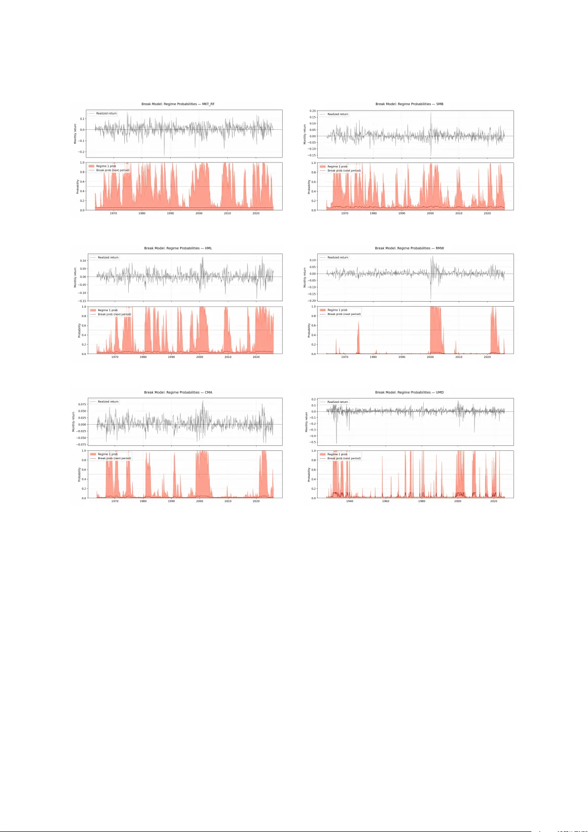
Mislearning of F actor Risk Premia under Structural Breaks A Missp eciﬁed Ba y esian Learning F ramew ork Yimeng Qiu Marc h 10, 2026 Abstract While asset-pricing mo dels increasingly recognize that factor risk premia are sub ject to structural change, existing literature t ypically assumes that in v estors correctly account for suc h instabilit y . This paper studies how in v estors instead learn under a missp eciﬁed mo del that underestimates structural breaks. W e prop ose a minimal Bay esian framework in whic h this misspeciﬁcation generates p ersisten t prediction errors and pricing distortions, and w e in tro duce an empirically tractable measure of mislearning intensit y (∆ t ) based on predictive lik eliho o d ratios. The empirical results yield three main ﬁndings. First, in benchmark factor systems, elev ated mislearning do es not forecast a deterministic short-run collapse in p erformance; in- stead, it is asso ciated with stronger long-horizon returns and Sharp e ratios, consistent with an equilibrium premium for acute mo del uncertain t y . Second, in a broader anomaly univ erse, this pricing relation do es not generalize uniformly: mislearning is more strongly asso ciated with future dra wdo wns, downside semiv olatilit y , and other measures of instability , with sub- stan tial heterogeneit y across anomaly families. Third, the cross-sectional relation b et w een instabilit y and mislearning is inheren tly conditional: while a monotonic link betw een break- proneness and a v erage mislearning do es not hold in the full cross-section, it re-emerges in lo w-friction (lo w-IV OL) en vironmen ts where break-state severit y is more comparable across assets. Finally , market structure aﬀects how mislearning is expressed in subsequen t outcomes: passiv e capital does not eliminate mislearning but shifts its manifestation aw a y from com- p ensation and to w ard realized risk and low er returns, with heterogeneous eﬀects across asset classes. Keyw ords: Behavioral ﬁnance; Ba y esian learning; Mo del missp eciﬁcation; Structural breaks; F actor risk premia; Relativ e en trop y JEL: G12, D83, C11, C32 1 Con ten ts 1 In tro duction 4 1.1 Measuring Mislearning . . . . . . . . . . . . . . . . . . . . . . . . . . . . . . . . . 4 1.2 T estable Predictions . . . . . . . . . . . . . . . . . . . . . . . . . . . . . . . . . . 4 1.3 Relation to Literature . . . . . . . . . . . . . . . . . . . . . . . . . . . . . . . . . 5 1.4 Mark et Structure and the Role of P assiv e Capital . . . . . . . . . . . . . . . . . . 5 1.5 Con tribution . . . . . . . . . . . . . . . . . . . . . . . . . . . . . . . . . . . . . . 5 2 T rue Pro cess: F actor Risk Premia with Structural Breaks 6 3 In v estor Beliefs: Missp eciﬁed Ba y esian Learning 6 4 Mislearning In tensit y 7 5 Asset Pricing Implications 8 6 Empirical Design 11 6.1 Data . . . . . . . . . . . . . . . . . . . . . . . . . . . . . . . . . . . . . . . . . . . 11 6.2 Estimating Predictive Densities . . . . . . . . . . . . . . . . . . . . . . . . . . . . 11 6.3 Baseline Predictive T ests . . . . . . . . . . . . . . . . . . . . . . . . . . . . . . . . 11 6.4 Cross-Sectional Diagnostics for Prop osition 4 . . . . . . . . . . . . . . . . . . . . 11 6.5 P assiv e Capital, Timing, and Institutional T ests . . . . . . . . . . . . . . . . . . . 12 6.5.1 Systemic Inv esting Proxies . . . . . . . . . . . . . . . . . . . . . . . . . . 12 6.5.2 Institutional T ests . . . . . . . . . . . . . . . . . . . . . . . . . . . . . . . 13 6.6 Inference in the Institutional Regressions . . . . . . . . . . . . . . . . . . . . . . . 13 7 Empirical Results 14 7.1 Descriptiv e Evidence . . . . . . . . . . . . . . . . . . . . . . . . . . . . . . . . . . 14 7.2 Cross-F actor Heterogeneit y . . . . . . . . . . . . . . . . . . . . . . . . . . . . . . 16 7.3 Baseline Predictive Regressions . . . . . . . . . . . . . . . . . . . . . . . . . . . . 16 7.4 q-F actor Robustness: Evidence from Hou–Xue–Zhang F actors . . . . . . . . . . . 18 7.5 q-F actor Cross-F actor Heterogeneity . . . . . . . . . . . . . . . . . . . . . . . . . 19 7.6 Anomaly-Univ erse Evidence . . . . . . . . . . . . . . . . . . . . . . . . . . . . . . 20 7.7 IV OL-Screened Cross-Sectional V alidation of Corollary 4.1 . . . . . . . . . . . . . 23 7.8 P assiv e Capital and Outcome Mapping . . . . . . . . . . . . . . . . . . . . . . . . 23 7.9 Additional Background T ables . . . . . . . . . . . . . . . . . . . . . . . . . . . . 25 8 Conclusion 25 A Additional F actor-Lev el Figures 27 A.1 Stable-Mo del Filtered States . . . . . . . . . . . . . . . . . . . . . . . . . . . . . 27 A.2 Break Probabilities . . . . . . . . . . . . . . . . . . . . . . . . . . . . . . . . . . . 28 A.3 Mislearning Series . . . . . . . . . . . . . . . . . . . . . . . . . . . . . . . . . . . 29 2 B F ull Predictive Regression T ables 29 B.1 Baseline Predictiv e Regressions (F ull) . . . . . . . . . . . . . . . . . . . . . . . . 29 B.2 Controlled Predictiv e Regressions (F ull) . . . . . . . . . . . . . . . . . . . . . . . 33 C Robustness Checks 36 C.1 Systemic Interaction with Mon th Fixed Eﬀects . . . . . . . . . . . . . . . . . . . 36 D Domestic-Equit y T argeting Diagnostics 36 E Passiv e Structure-Shift Diagnostics in the Anomaly Universe 42 F FF6 Revised Cross-F actor Diagnostic 47 G Benc hmark Non-Absorb er Diagnostics 47 H Additional Mo del-Fit T ables 48 I Mathematical Pro ofs 49 I.1 Pro of of Prop osition 1: Slow Up dating after Breaks . . . . . . . . . . . . . . . . . 49 I.2 Additional F ormal Results for Prop ositions 2–4 . . . . . . . . . . . . . . . . . . . 50 J q-F actor Robustness T ables 55 J.1 Unrestricted Baseline . . . . . . . . . . . . . . . . . . . . . . . . . . . . . . . . . . 55 J.2 Common-Sample Baseline . . . . . . . . . . . . . . . . . . . . . . . . . . . . . . . 57 J.3 Con trolled Sp eciﬁcation . . . . . . . . . . . . . . . . . . . . . . . . . . . . . . . . 60 J.4 Rank-Based Diagnostic for Prop osition 4 . . . . . . . . . . . . . . . . . . . . . . . 63 K Anomaly F amily Classiﬁcation and Mo del Diagnostics 63 L Reduced-F orm Cross-Sectional Diagnostics for Prop osition 4 68 M IV OL-Screened V alidation of Corollary 4.1 70 N Additional Anomaly-Univ erse Predictiv e Diagnostics 71 3 1 Introduction Empirical asset pricing studies rep eatedly do cumen t that factor risk premia are time-v arying and sub ject to structural instabilit y . Allowing for structural breaks often leads to rejection of the assumption of stable premia. F or e xample, Smith and Timmermann ( 2022 ) do cument discrete breaks in cross-sectional risk premia and show that several classic factor premia decline in the later sample. Similarly , Chib ( 2024 ) ﬁnd that allo wing for multiple breaks substan tially reduces the set of priced factors. This pap er asks a b ehavioral question: how do investors le arn ab out factor risk pr emia in envir onments with structur al change? W e prop ose a minimal framew ork of missp e ciﬁe d Bayesian le arning . In v estors follo w Ba y esian up dating but op erate under an incorrect mo del class. Sp eciﬁcally , they ﬁlter the price of risk assuming a stable low-drift pro cess while the true process contains o ccasional structural shifts. When structural c hanges o ccur, the Kalman gain under the stable mo del is to o small, leading to slo w b elief adjustmen t. This generates p ersisten t prediction errors and mispricing. 1.1 Measuring Mislearning W e in tro duce an empirically tractable measure of mislearning intensit y based on predictiv e densit y comparisons b et w een tw o mo dels: • a stable mo del , in terpreted as the in v estor’s b elief system; and • a break mo del , in terpreted as the researc her’s b enchmark for structural instabilit y . The log predictiv e likelihoo d ratio b etw een the tw o mo dels approximates relativ e entrop y (KL divergence) and serv es as a measure of mislearning. 1.2 T estable Predictions The mo del generates three main predictions: (1) Mislearning spikes around structural breaks. (2) High mislearning predicts w eak short-horizon p erformance and, in b enchmark factor sys- tems, can b e asso ciated with a higher future Sharp e ratio ov er longer horizons, consistent with an uncertaint y premium. In broader anomaly univ erses, where limits to arbitrage and price-impact frictions are more sev ere , the same state v ariable ma y instead load more strongly on future instabilit y and do wnside risk than on unconditional Sharp e ratios. (3) F actors with more unstable risk premia exhibit greater misle arning exp osur e , though this exp osure need not b e one-dimensional. In particular, break frequency and break-state sev erit y may v ary indep enden tly across factor taxonomies. As a result, the mapping from break-proneness to a verage mislearning is inheren tly conditional and may not app ear as a uniform monotonic relation in the presence of cross-sectional heterogeneit y in break-state sev erit y . In addition, market structure may alter ho w mislearning is expressed in subse- quen t outcomes: passive intensit y need not dampen mislearning p ersistence uniformly , but 4 ma y shift whether elev ated mislearning is follo wed by comp ensation, by low er cumulativ e returns, or b y future risk. 1.3 Relation to Literature Our framew ork diﬀers from rational learning mo dels suc h as V eronesi ( 1999 ), whic h assume correctly sp eciﬁed mo dels. Instead, inv estors op erate within a missp eciﬁed mo del class. The framew ork is related to b ehavioral mo dels suc h as Barb eris et al. ( 1998 ) but fo cuses on structural instabilit y in factor premia. More broadly , the pap er sp eaks to the literature on disapp earing or unstable risk premia, mo del uncertain t y , and b elief-based asset pricing. Relative to recent work on time-v arying factor premia, our emphasis is not merely that premia v ary ov er time, but that a stable learning rule can b ecome systematically wrong when the underlying data-generating pro cess exp eriences discrete shifts. 1.4 Mark et Structure and the Role of P assiv e Capital A cen tral question in mo dern market structure is whether the gro wth of passive and other rule-based capital changes how pricing errors are transmitted across mark ets. Our evidence in- dicates that passiv e capital primarily aﬀects ho w elev ated mislearning is expressed in subsequen t outcomes rather than whether mislearning arises in the ﬁrst place. Within both the FF6 and q5 factor systems, higher passive intensit y is asso ciated with w eak er future Sharp e comp ensation, lo wer future cum ulativ e returns, and stronger realization of forw ard-lo oking risk. In the broader anomaly univ erse, the same institutional force is more heterogeneous and app ears through partial family-level structure shifting. W e therefore in- terpret passive capital as a conditional mark et-structure mo diﬁer that helps determine whether mislearning is comp ensated or realized through subsequent instabilit y . 1.5 Con tribution The pap er mak es three con tributions. First, it pro vides a minimal missp eciﬁed-learning asset-pricing framew ork that d irectly maps structural instabilit y in factor risk premia into a measurable state v ariable. The framework sho ws how slow b elief up dating under mo del missp eciﬁcation generates p ersisten t prediction errors and pricing distortions follo wing structural breaks. Second, it delivers a structural reinterpretation of the cross-sectional relation b et w een insta- bilit y and mislearning. Prop osition 4 shows that unconditional mislearning arises from tw o dis- tinct components: the frequency of structural breaks and the sev erity of mislearning conditional on break states. A stronger implication (Corollary 4.1) predicts a monotonic relation b etw een break-proneness and av erage mislearning when break-state severit y is comparable across assets. Empirically , this condition fails in the full cross-section. W e show that this failure is driven b y systematic heterogeneit y in break-state sev erit y . In particular, idiosyncratic v olatility (IV OL), a standard proxy for limits to arbitrage, strongly predicts break-state severit y ( µ 1 ,k ) but has no predictiv e p ow er for break frequency ( π k ). This separation allows us to use IVOL as an ex-ante 5 screening v ariable: in low-IV OL (low-friction) environmen ts, where severit y is more homoge- neous, the monotonic relation b et ween break-proneness and mislearning re-emerges, whereas it breaks do wn in high-IVOL environmen ts. These results establish that the cross-sectional implications of mislearning are inheren tly conditional on the limits-to-arbitrage environmen t. Third, it pro vides an empirical implemen tation based on predictiv e density comparisons and do cumen ts how mislearning maps into future outcomes. In b enc hmark factor systems, elev ated mislearning is associated with stronger long-horizon returns and Sharpe ratios, consisten t with an uncertain t y premium. In a broader anomaly univ erse, mislearning is instead more strongly link ed to future instability , including drawdo wns and do wnside semiv olatilit y , with substan tial heterogeneit y across anomaly families. Rather than eliminating mislearning, passiv e capital mo diﬁes how mislearning is transmitted in to subsequen t outcomes. 2 T rue Pro cess: F actor Risk Premia with Structural Breaks Consider K factor returns. T o prop erly align the state transition with the observ ation timing in a standard state-space form ulation, we sp ecify: f t +1 = λ t +1 + u t +1 , u t +1 ∼ N (0 , Σ u ) , (1) where λ t +1 represen ts the conditional exp ected factor return driving the realization at t + 1 (suc h that E t [ f t +1 ] = E t [ λ t +1 ]). The true state evolution is λ t +1 = Aλ t + η t +1 + J t +1 , (2) where η t +1 ∼ N (0 , Σ η ) and J t +1 represen ts structural breaks: J t +1 =    0 with probability 1 − p, ζ t +1 with probability p, ζ t +1 ∼ N ( µ J , Σ J ) . (3) This sp eciﬁcation captures a simple but empirically relev an t environmen t: most of the time exp ected premia ev olve gradually , but o ccasionally they shift discretely due to c hanges in macro conditions, inv estor clientele, market structure, or factor crowding. 3 Inv estor Beliefs: Missp eciﬁed Bay esian Learning In v estors observe factor returns but b eliev e that the latent state ev olv es smo othly without jumps: f t +1 = λ t +1 + u t +1 , u t +1 ∼ N (0 , Σ u ) , (4) λ t +1 = Aλ t + ˜ η t +1 , ˜ η t +1 ∼ N (0 , ˜ Σ η ) , (5) with the crucial missp eciﬁcation that: ˜ Σ η ≪ Σ η , (6) 6 and no explicit jump component. Th us in vestors are Ba yesian, but within a missp eciﬁed model class: they underestimate state v olatilit y and ignore the possibility of breaks. Under this b elief system, p osterior b eliefs follo w the standard Kalman ﬁlter. Let λ t | F t ∼ N ( ˆ λ t , P t ) , (7) where F t = σ ( f 1 , . . . , f t ). The belief recursion is ˆ λ t +1 | t = A ˆ λ t , (8) P t +1 | t = AP t A ⊤ + ˜ Σ η , (9) K t +1 = P t +1 | t  P t +1 | t + Σ u  − 1 , (10) ˆ λ t +1 = ˆ λ t +1 | t + K t +1  f t +1 − ˆ λ t +1 | t  , (11) P t +1 = ( I − K t +1 ) P t +1 | t . (12) Because ˜ Σ η is to o small, the steady-state Kalman gain K is too small, and b elief adjustmen t is to o slo w following a structural shift. 4 Mislearning In tensit y Deﬁne the one-step-ahead predictive densities under the t w o models for the realized return at time t , conditional strictly on prior information F t − 1 : p S ( f t | F t − 1 ) and p B ( f t | F t − 1 ) , where S denotes the stable inv estor-belief mo del and B denotes the break-aw are benchmark. The mislearning measure, ev aluated at the end of p erio d t , is ∆ t = log p B ( f t | F t − 1 ) p S ( f t | F t − 1 ) . (13) By deﬁning ∆ t strictly using information up to time t , w e ensure that the state v ariable is fully observ able at the time of p ortfolio formation, eﬀectively eliminating an y lo ok-ahead bias when predicting future p erformance P erf t → t + h . Large p ositive ∆ t indicates that the stable model assigns muc h lo w er probability to the realized return than the break mo del do es. In that sense, ∆ t measures the severit y of lo cal mo del missp eciﬁcation. A rolling v ersion is also useful to capture persistent regimes: ∆ t ( m ) = 1 m m − 1 X j =0 ∆ t − j . (14) 7 5 Asset Pricing Implications T o formalize the pricing distortions induced b y mislearning, w e em b ed the ﬁltering problem in to a stylized equilibrium framework. Consider a market with a risk-free asset and K risky factors. A represen tativ e in vestor has constant absolute risk a v ersion (CARA) with a co eﬃcien t γ and maximizes exp ected utilit y ov e r next-p erio d w ealth. Assume that f t +1 denotes the vector of risky factor excess returns and that the inv estor solv es a one-p erio d CARA-normal portfolio problem. Under the sub jective stable model, E S t [ f t +1 ] = E S t [ λ t +1 ] = A ˆ λ t . Strictly sp eaking, the inv estor’s conditional cov ariance matrix of returns is V ar S t ( f t +1 ) = P t +1 | t + Σ u , where P t +1 | t is the ﬁltered state uncertain t y . F or tractabilit y , how ev er, we abstract from state- uncertain t y v ariation in p ortfolio demand and approximate the sub jective return cov ariance by Σ u alone. Equiv alen tly , w e treat ﬁltered state uncertaint y as second order relative to pay oﬀ noise, i.e. P t +1 | t ≪ Σ u . Under this approximation, the inv estor’s optimal p ortfolio demand v ector at time t is x t = 1 γ Σ − 1 u E S t [ f t +1 ] = 1 γ Σ − 1 u A ˆ λ t , (15) where γ is the co eﬃcien t of absolute risk a version. T o endogenize the time-v arying nature of the true risk premium λ t , w e introduce a time- v arying, exogenous supply of factor assets, S t , which can be in terpreted as mechanical capital ﬂo ws or noise trader demand (e.g., rigid rebalancing by the passive index funds discussed in Section 1.4 ). The market clearing condition requires x t = S t , which implies that the sub jectiv e risk premium required to clear the mark et is: A ˆ λ t = γ Σ u S t (16) Crucially , supp ose the unobserved true supply follows S t = ¯ S + ν t , where the supply sho ck ν t o ccasionally experiences discrete structural shifts due to sudden institutional allo cation c hanges. Consequen tly , the true market-clearing exp ected risk premium, Aλ true t = γ Σ u S t , follo ws the jump-augmen ted process sp eciﬁed in our state equations. The inv estor, ho w ev er, observes realized returns and ﬁlters the laten t state under the missp eciﬁed b elief that supply (and th us the premium) ev olv es smoothly without jumps. This mec hanism generates a p ersistent b elief w edge, ˆ λ t  = λ true t , leading to systematic pricing errors and predictable subsequen t return reversals. Prop osition 1 (Slow up dating after breaks) . Supp ose the true pr o c ess fol lows ( 2 ) – ( 3 ) , while investors ﬁlter using ( 4 ) – ( 6 ) . If a nonzer o br e ak o c curs at time t ⋆ , then the p osterior me an err or ˆ λ t − λ t r emains systematic al ly biase d for multiple p erio ds after t ⋆ . The p ersistenc e of this bias incr e ases as ˜ Σ η b e c omes smal ler. Se e App endix I for the formal pr o of. 8 Prop osition 2 (Mislearning spikes near structural breaks) . When r e alize d r eturns ar e mor e c on- sistent with the pr e dictive density of the br e ak mo del than that of the stable mo del, misle arning intensity (∆ t ) rises. This incr e ase is monotonic al ly lar ger when the me an shift of the structur al br e ak is lar ger. F urthermor e, c onditional on a suﬃciently lar ge br e ak-c onsistent r e al- ization , a mor e rigid stable mo del (i.e., a smal ler subje ctive state varianc e) strictly magniﬁes the likeliho o d gap and pr o duc es lar ger misle arning spikes. Prop osition 3 (Uncertain t y Premium and F uture Performance) . When misle arning intensity ( ∆ t ) spikes fol lowing a structur al br e ak, the asset enters a r e gime of elevate d mo del unc ertainty and b elief diver genc e. In e quilibrium, investors demand a higher risk pr emium to c omp ensate for this ambiguity. Conse quently, while ∆ t exhibits only we ak pr e dictive p ower for futur e r e alize d volatility prior to standar d risk c ontr ols, it is asso ciate d with elevate d futur e Sharp e r atios in long-horizon r e gr essions. This dynamic r eﬂe cts an e quilibrium c omp ensation for acute mo del risk, r ather than a deterministic c ol lapse in short-term factor p erformanc e. Interpr etation and sc op e: low-friction b enchmark and outc ome bifur c ation. T o clarify wh y the pricing implication in Prop osition 3 need not generalize uniformly across assets, consider the equilibrium exp ected return decomp osition established in Appendix I (Theorem 1): E t [ d t +1 − q t ] = w t + γ Σ u S t , (17) where w t denotes the belief w edge and γ Σ u S t captures the price-impact component of exogenous supply sho cks. Prop osition 3 is most naturally in terpreted as a lo w-friction b enc hmark : when the price-impact comp onent remains small relativ e to the gradual correction embo died in w t , elev ated mislearning is resolved primarily through b elief adjustment and app ears as a comp ensated uncertaint y premium. When limits to arbitrage are more severe, how ever, the same mislearning sho ck need not b e expressed through future Sharp e comp ensation. If the price-impact comp onen t b ecomes suﬃ- cien tly important re lativ e to the belief-correction component, elev ated mislearning is more lik ely to b e realized through price dislo cation, realized volatilit y , drawdo wns, downside semivolatil- it y , or broader instabilit y . This distinction provides a mo del-consistent interpretation of why the b enc hmark factor systems are more consistent with an uncertaint y-premium mechanism, whereas the broader anomaly univ erse more often reﬂects the instabilit y channel. Empirically , the IV OL-screened cross-sectional tests b elow exploit this logic b y using IVOL as a reduced-form pro xy for en vironmen ts in whic h the lo w-friction b enchmark is more or less lik ely to hold. Prop osition 4 (Cross-factor mislearning exp osure: decomp osition) . L et B k,t denote the br e ak- state indic ator for factor k , and deﬁne π k = Pr( B k,t = 1) , µ 1 ,k = E [∆ k,t | B k,t = 1] , µ 0 ,k = E [∆ k,t | B k,t = 0] . Then the unc onditional aver age misle arning exp osur e of factor k satisﬁes E [∆ k,t ] = π k µ 1 ,k + (1 − π k ) µ 0 ,k . 9 Mor e over, for any ﬁxe d spike thr eshold c , Pr(∆ k,t > c ) = π k q 1 ,k ( c ) + (1 − π k ) q 0 ,k ( c ) , wher e q 1 ,k ( c ) = Pr(∆ k,t > c | B k,t = 1) , q 0 ,k ( c ) = Pr(∆ k,t > c | B k,t = 0) . Thus cr oss-factor variation in unc onditional misle arning c an arise thr ough either br e ak fr e quency or br e ak-state severity, and the same is true for the fr e quency of lar ge misle arning spikes. This de c omp osition holds without imp osing any r estriction on the r elation b etwe en br e ak fr e quency and br e ak-state severity acr oss factors. Corollary 4.1 (Conditional monotone exp osure) . Supp ose the non-br e ak c omp onent of mis- le arning is c omp ar able acr oss factors, so that µ 0 ,k = ¯ µ 0 , and deﬁne the br e ak-state severity gap δ k := µ 1 ,k − µ 0 ,k . If δ k ≥ 0 for al l k and δ k is c onstant acr oss factors or we akly incr e asing in π k , then E [∆ k,t ] is we akly incr e asing in π k . Likewise, for any ﬁxe d thr eshold c , if q 0 ,k ( c ) = ¯ q 0 ( c ) and η k ( c ) := q 1 ,k ( c ) − q 0 ,k ( c ) ≥ 0 is c onstant acr oss factors or we akly incr e asing in π k , then Pr(∆ k,t > c ) is we akly incr e asing in π k . This r esult pr ovides a suﬃcient c ondition r ather than a ne c essary one. Empiric al interpr etation. Proposition 4 implies that cross-factor av erage mislearning can diﬀer b ecause factors break more often, b ecause mislearning is more severe conditional on break states, or b oth. Corollary 4.1 adds a stronger suﬃcien t condition under whic h break-proneness maps monotonically into a v erage mislearning and spike frequency . In the data, this stronger implication need not hold uniformly across the full cross-section b ecause the break-state sev erit y gap can itself be heterogeneous. A practical screening v ariable for this heterogeneit y is the limits-to-arbitrage environmen t. In particular, App endix L shows that IVOL predicts break- state conditional severit y µ 1 ,k but do es not predict break-proneness π k . This motiv ates using IV OL-sorted subsamples to ev aluate where the corollary is more lik ely to hold empirically . Remark 1 (Cross-sectional implication) . Pr op osition 4 shows that onc e cr oss-factor heter o- geneity in br e ak-state severity is admitte d, the low-friction b enchmark in Pr op osition 3 ne e d not gener alize uniformly acr oss assets. The empiric al analysis exploits this distinction by us- ing IVOL as a r e duc e d-form pr oxy for the limits-to-arbitr age envir onment, ther eby identifying settings in which the c onditional monotonic implic ation in Cor ol lary 4.1 is mor e likely to hold. Remark 2 (P assiv e Capital as a Mark et-Structure Mo diﬁer) . While active, b ounde d ly r ational investors ar e susc eptible to p ersistent misle arning during structur al br e aks, p assive or systemic c apital may aﬀe ct how such misle arning is r eﬂe cte d in subse quent pric es and p ayoﬀs. Empiri- c al ly, we ther efor e test not only whether p assive intensity damp ens p ost-br e ak misle arning p er- sistenc e, but also whether it changes whether elevate d misle arning is fol lowe d by c omp ensation, lower cumulative r eturns, downside risk, or br o ader instability. 10 6 Empirical Design 6.1 Data The empirical implementation relies primarily on public monthly factor return data: MKT-RF, SMB, HML, RMW, CMA, and UMD. The core factor dataset is supplemen ted by volatilit y con trols and a passive-in v esting proxy constructed from ICI data. 6.2 Estimating Predictiv e Densities Tw o mo dels are estimated for each factor: • a stable state-space mo del estimate d via Kalman ﬁltering; and • a break-allowing mo del estimated as a Mark o v-switc hing b enchmark. The stable mo del produces one-step-ahead predictiv e densit y p S ( f t | F t − 1 ), while the break mo del pro duces p B ( f t | F t − 1 ). These directly feed in to the construction of ∆ t in ( 13 ). 6.3 Baseline Predictiv e T ests The baseline predictiv e sp eciﬁcation is P er f t → t + h = a + b ∆ t + ϵ t + h , (18) where P er f t → t + h denotes future p erformance ov er horizon h , such as future cumulativ e return, future Sharp e ratio, future realized volatilit y , or a tail-even t indicator. Con trolled sp eciﬁcations add standard risk controls, such as rolling volatilit y and market uncertain t y . All forward outcome v ariables are constructed to exclude the con temp oraneous return at time t . In dense monthly b enc hmark panels, this corresponds closely to the calendar in terv al from t + 1 on w ard. In broader anomaly panels with occasional missing observ ations, the forw ard horizon is formed from the next av ailable return observ ations after t . This preserves the no-lo ok-ahead timing of the predictiv e design ev en when the realized forward window is not a p erfectly con tiguous calendar block in calendar time. 6.4 Cross-Sectional Diagnostics for Prop osition 4 T o ev aluate Proposition 4 and Corollary 4.1 in the anomaly univ erse, w e construct anomaly-level cross-sectional ob jects from the break-probability and mislearning panels. F or each anomaly k , w e deﬁne break-proneness π k = 1 T k X t Pr( B k,t = 1) , whic h we in terpret as the empirical counterpart of the theoretical break probability . W e further deﬁne break-state conditional mislearning sev erit y as µ 1 ,k = P t Pr( B k,t = 1)∆ k,t P t Pr( B k,t = 1) , 11 and the corresp onding non-break component as µ 0 ,k = P t (1 − Pr( B k,t = 1))∆ k,t P t (1 − Pr( B k,t = 1)) . W e also compute the unconditional av erage mislearning of each anomaly as the full-sample mean of ∆ k,t . T o study when the conditional monotonic implication in Corollary 4.1 is more likely to hold, w e construct an anomaly-level limits-to-arbitrage proxy based on mon thly return data. Specif- ically , IV OL is measured as the standard deviation of residuals from a time-series regression of each anomaly’s return on the F ama–F rench three factors. Reduced-form cross-sectional di- agnostics then ev aluate whether IVOL is asso ciated with break-state conditional severit y µ 1 ,k , with break-proneness π k , or with b oth. F ull reduced-form results are rep orted in Appendix L , while the IV OL-tertile v alidation of Corollary 4.1 is rep orted in Section 7.7 and App endix M . 6.5 P assiv e Capital, Timing, and Institutional T ests W e study whether market structure, as proxied b y passive capital, c hanges how mislearning is reﬂected in subsequen t outcomes. The passive v ariables used here should b e in terpreted as macro-lev el proxies for the prev alence of rule-based capital rather than as direct measures of passiv e trading or p ortfolio holdings. 6.5.1 Systemic In v esting Pro xies W e use man ually collected data from the In v estmen t Company Institute’s (ICI) Long-T erm F und T rends report. Our ﬁnal matched sample spans 121 mon ths, from January 2016 to January 2026. Baseline Measure Our primary level pro xy is the total index-fund asset share, denoted as P assiv eS har e T otal t , which represents the fraction of total fund assets managed under passiv e indexing strategies. During our sample p erio d, this aggregate measure rises substan tially from 28.45% to 52.69%. Detrended Measure T o isolate shorter-run ﬂuctuations in passiv e in tensity from its sec- ular trend, w e construct a detrended pro xy , P assiv eS har e Detr ended t , using a strictly one-side d Ho dric k–Prescott ﬁlter with mon thly smo othing parameter λ = 129 , 600. A t eac h date, the cycli- cal component is computed using only information a v ailable up to that date, thereb y a v oiding the lo ok-ahead bias inherent in standard t w o-sided HP ﬁltering. Domestic-Equit y Measure for T argeting Diagnostics F or supplemen tary targeting ex- ercises, we also construct a domestic-equity passiv e share, P assiv eS har e DomE q t , deﬁned anal- ogously to the total passive share but restricted to the domestic-equity fund univ erse. Where needed for appendix targeting diagnostics, w e additionally construct a detrended domestic- equit y analogue using the same strictly one-sided HP procedure. 12 Timing and Alignmen t Because publication-lag metadata for the ICI releases are not fully a v ailable in the current implemen tation, our baseline institutional regressions use lagge d p assive pr oxies (i.e., information av ailable at t − 1 when forming predictions at t ). Same-month passive sp eciﬁcations are retained only as robustness chec ks and are not used as the pap er’s primary institutional evidence, since their real-time av ailability is more diﬃcult to v erify . Data Processing and P anel In tegration The ICI series are standardized to end-of-mon th timestamps and merged on to the factor and anomaly panels b y mon th. These proxies are not winsorized or standardized further. Their economic magnitudes are preserved. 6.5.2 Institutional T ests W e distinguish b et w een t wo empirical c hannels. (i) Break-Onset In teraction As a b enchmark, we ﬁrst test whether passiv e capital is asso- ciated with larger or smaller contemporaneous mislearning at break onset: ∆ k,t = a k + b B r eak k,t + c S y stemicI ntensity t − 1 + d ( B r eak k,t × S y stemicI ntensity t − 1 ) + ϵ k,t . (19) A negativ e co eﬃcien t on the in teraction term d w ould b e consisten t with con temp oraneous buﬀering, whereas a non-negative co eﬃcien t is more consistent with non-buﬀering or mild am- pliﬁcation. (ii) Outcome-Mapping In teraction Our main institutional test asks whether passive cap- ital changes how elev ated mislearning is expressed in subsequen t outcomes: P er f k,t → t + h = a k + b ∆ k,t + c S y stemicI ntensity t − 1 + d (∆ k,t × S y stemicI ntensity t − 1 )+ X ′ t θ + ϵ k,t + h , (20) where P er f k,t → t + h includes future Sharp e ratios, cum ulative returns, and forw ard-looking risk outcomes such as dra wdo wns and do wnside semivolatilit y . The co eﬃcien t d identiﬁes whether passive intensit y changes the mapping from mislearning in to future comp ensation or future risk. This mapping-based c hannel b ecomes the pap er’s cen tral institutional test once persistence-based absorb er evidence pro ves w eak and sample- sensitiv e. Iden tiﬁcation Note Because passiv e pro xies v ary only o ver time and are common across factors within a month, mon th ﬁxed eﬀects w ould absorb the passiv e-share main eﬀect and materially w eak en identiﬁcation of the mapping sp eciﬁcations. W e therefore rep ort baseline institutional regressions without month ﬁxed eﬀects. 6.6 Inference in the Institutional Regressions Because several forward outcomes ov erlap ov er 12-month horizons, institutional interaction regressions ma y inherit serial dep endence from ov erlapping observ ations. In the baseline 13 b enc hmark-factor predictiv e tables, we contin ue to rep ort the pap er’s standard inference con v en tion. F or the passiv e-extension cum ulative-return diagnostics and the larger anomaly- univ erse interaction exercises, we additionally rely on ov erlap-robust or dep endence-robust inference, including HAC or clustering-based pro cedures where appropriate. Accordingly , the institutional in terpretation is based not only on individual p -v alues from any single sp eciﬁca- tion, but also on the consistency of the sign pattern across systems, outcomes, and inference con v en tions. In particular, the cumulativ e-return interaction results pro vide the cleaner con- ﬁrmation that passive weak ens comp ensation itself rather than merely altering risk-adjusted p erformance. 7 Empirical Results 7.1 Descriptiv e Evidence Figure 1 plots the mon thly factor return series used in the analysis. The six factors display substan tial time v ariation, o ccasional large dislo cations, and pronounced heterogeneity across st yles. 14 Figure 1: Mon thly factor return series for the six b enc hmark factors. 15 T o keep the main text concise, the factor-b y-factor ﬁltered-state plots, break-probability plots, and full ∆ t series are rep orted in Appendix A . 7.2 Cross-F actor Heterogeneity W e b egin with the FF6 factor set and ev aluate b oth Prop osition 4 and Corollary 4.1 . Prop o- sition 4 itself is a decomp osition result: cross-factor diﬀerences in unconditional mislearning can arise through break frequency , break-state severit y , or b oth. Corollary 4.1 adds a stronger suﬃcien t condition under whic h more break-prone factors also exhibit higher av erage mislearn- ing and more frequent large-mislearning spikes. Empirically , ho wev er, this stronger monotonic implication need not hold cleanly if break-state severit y diﬀers materially across factors. T o ev aluate this implication more symmetrically , T able 1 rep orts a revised FF6 heterogeneit y summary . F or eac h FF6 factor, the table reports: (i) the full-sample mean break probabilit y , (ii) the share of mon ths classiﬁed as break states using a p osterior break-probabilit y threshold of 0.5, (iii) the av erage mislearning intensit y conditional on break mon ths, (iv) spike frequency based on a p o oled 90th-p ercentile threshold of ∆ t , and (v) the 12-month future-Sharp e co eﬃcient from the relev an t predictiv e speciﬁcation. The revised FF6 evidence supp orts the presence of substantial cross-factor heterogeneity , but it also shows that the relation b etw een break-proneness and a verage mislearning severit y is not p erfectly monotone. Some factors en ter break states more frequen tly , while others exhibit more severe conditional mislearning once in the break state. This implies that break frequency and break-state sev erit y are empirically distinct dimensions. Accordingly , the FF6 evidence is somewhat more supp ortive than the q5 case, but it still suggests that the stronger monotonic implication in Corollary 4.1 should b e in terpreted with caution. T able 1: FF6 factors: break diagnostics and predictive slop es F actor Pr(Break) Break share ∆ (break) Spike freq Sharp e co ef. ( p , 12m) Obs. Break mths MKT (RF) 0.4878 0.4660 -0.0237 0.0360 0.2887 (0.0005) 751 350 SMB 0.3423 0.2716 0.0570 0.0253 -0.0843 (0.2074) 751 204 HML 0.3664 0.3409 0.0578 0.0466 0.2333 (0.0044) 751 256 RMW 0.1019 0.0985 1.2098 0.0293 0.0710 (0.0028) 751 74 CMA 0.2436 0.2210 0.1994 0.0453 -0.0049 (0.9517) 751 166 UMD 0.1569 0.1312 0.7763 0.3011 -0.0057 (0.8031) 1189 156 7.3 Baseline Predictiv e Regressions T able 2 rep orts a condensed baseline sp eciﬁcation that retains only p o oled estimates (core results). T able 3 rep orts the corresp onding condensed con trolled sp eciﬁcation. 16 T able 2: Baseline po oled predictiv e regressions of future factor p erformance on mislearning in tensit y ∆ t . Outcome Horizon Co ef. (SE, t , p ) Obs. ( R 2 ) Panel A. Horizon = 3 months Sharp e 3 0.0102 (0.0476, 0.21, 0.831) 4926 (0.0108) Cum. return 3 -0.0012 (0.0027, -0.42, 0.673) 4926 (0.0076) V olatility 3 0.0061 (0.0037, 1.64, 0.100) 4926 (0.1260) Do wnside v ol. 3 -0.0006 (0.0004, -1.28, 0.200) 4926 (0.0154) Max DD 3 -0.0001 (0.0004, -0.24, 0.808) 4926 (0.0258) Panel B. Horizon = 6 months Sharp e 6 0.0226 (0.0251, 0.90, 0.368) 4908 (0.0263) Cum. return 6 0.0002 (0.0032, 0.06, 0.951) 4908 (0.0135) V olatility 6 0.0043 (0.0028, 1.56, 0.120) 4908 (0.1631) Do wnside v ol. 6 0.0039 (0.0036, 1.07, 0.285) 4908 (0.0555) Max DD 6 -0.0004 (0.0007, -0.64, 0.524) 4908 (0.0495) Panel C. Horizon = 12 months Sharp e 12 0.0288 (0.0219, 1.31, 0.189) 4872 (0.0382) Cum. return 12 0.0040 (0.0049, 0.82, 0.415) 4872 (0.0255) V olatility 12 0.0036 (0.0019, 1.89, 0.059) 4872 (0.2091) Do wnside v ol. 12 0.0033 (0.0025, 1.33, 0.185) 4872 (0.1216) Max DD 12 0.0000 (0.0013, -0.06, 0.955) 4872 (0.0799) T able 3: Controlled p o oled predictiv e regressions with additional risk con trols. Outcome Horizon Co ef. (SE, t , p ) Obs. ( R 2 ) Panel A. Horizon = 3 months Sharp e 3 0.0769 (0.0887, 0.87, 0.386) 2580 (0.0187) Cum. return 3 0.0024 (0.0019, 1.23, 0.218) 2580 (0.0236) V olatility 3 0.0021 (0.0014, 1.45, 0.148) 2580 (0.2887) Do wnside v ol. 3 -0.0008 (0.0011, -0.79, 0.428) 2580 (0.0413) Max DD 3 0.0001 (0.0007, 0.16, 0.876) 2580 (0.0786) Panel B. Horizon = 6 months Sharp e 6 0.0521 (0.0438, 1.19, 0.234) 2562 (0.0489) Cum. return 6 0.0034 (0.0031, 1.09, 0.274) 2562 (0.0403) V olatility 6 0.0012 (0.0018, 0.66, 0.510) 2562 (0.3916) Do wnside v ol. 6 -0.0005 (0.0015, -0.30, 0.761) 2562 (0.1336) Max DD 6 -0.0006 (0.0011, -0.55, 0.580) 2562 (0.1322) Panel C. Horizon = 12 months Sharp e 12 0.0801 (0.0288, 2.78, 0.006) 2526 (0.0735) Cum. return 12 0.0145 (0.0048, 3.00, 0.003) 2526 (0.0789) V olatility 12 0.0009 (0.0017, 0.51, 0.608) 2526 (0.4163) Do wnside v ol. 12 -0.0017 (0.0015, -1.16, 0.248) 2526 (0.2734) Max DD 12 -0.0040 (0.0016, -2.52, 0.012) 2526 (0.1594) 17 Economic In terpretation of Predictiv e Regressions: Con trary to the naive h yp othesis that mislearning mechanically leads to a p ersistent deterioration in short-term factor returns, the bias-free results in T able 3 rev eal a comp elling long-term equilibrium dynamic. In the short run ( h = 3 , 6), the predictiv e co eﬃcien ts on returns and Sharp e ratios are statistically indistinguishable from zero, reﬂecting the noisy and turbulen t nature of b elief adjustments immediately following a regime shift. How ev er, o v er a longer in v estmen t horizon ( h = 12), w e document a highly signiﬁcant p ositive relationship b et w een ∆ t and both future cum ulativ e returns ( p = 0 . 002) and future Sharpe ratios ( p = 0 . 005). This empirical ﬁnding strongly supp orts an uncertain ty premium mechanism : when mo del missp eciﬁcation is sev ere, the p erceiv ed am biguity of the asset’s true data-generating pro cess forces the mark et to price in a substan tial risk premium. Therefore, p eriods of high mislearning act as pro xy indicators for elev ated mo del uncertaint y , whic h are subsequently comp ensated b y higher risk-adjusted returns ov er a one-y ear horizon. Complete factor-level results are mov ed to App endix B and split in to separate tables by horizon ( h = 3 , 6 , 12) for readability . 7.4 q-F actor Robustness: Evidence from Hou–Xue–Zhang F actors T o assess whether the empirical insights dep end on the sp eciﬁc factor taxonomy , we re-estimate the entire mislearning pipeline on the Hou–Xue–Zhang q5 factor set (mark et, size, inv estment, proﬁtabilit y , and expected growth). W e compute q5-based mislearning series, estimate predic- tiv e regressions, and compare unrestricted baseline, common-sample baseline, and con trolled sp eciﬁcations. The q5 factor returns are obtained from the oﬃcial Global-Q data library , which curren tly pro vides q-factor and q5 factor returns in the 1967–2024 sample, together with a tech- nical do cumen t describing the construction of the factors. The pass iv e-in v esting measures are compiled from the oﬃcial ICI Monthly Activ e and Index Data releases and the corresp onding Activ e and Index In v esting statistical rep orts.( Global-Q , 2025a , b ; Hou, Mo, Xue, and Zhang , 2021 ; Inv estmen t Company Institute , 2026a , b ) Sev eral patterns emerge. First, the state-v ariable property is preserv ed: mislearning exhibits little predictive pow er for 3- or 6-mon th outcomes, consisten t with the view that acute mo del uncertain t y is not immediately priced. Second, at the 12-mon th horizon, the p o oled co eﬃcien ts retain a p ositiv e tilt, esp ecially for future Sharp e ratios, suggesting that ele v ated mislearning is associated with a longer-horizon uncertaint y premium. Third, this long-horizon tilt survives when the baseline is restricted to the common-sample window, indicating that it is not merely an artifact of diﬀering sample lengths. At the same time, the p ositive long-horizon relation is not uniformly shared across all q-factors, and is strongest for the mark et q-factor. Ov erall, the q5 analysis lends partial but meaningful supp ort to the dynamic pricing inter- pretation of mislearning. It conﬁrms the state-v ariable and long-horizon uncertain t y-premium dimensions of the mec hanism while also highligh ting substan tial heterogeneit y across alternative factor taxonomies. The full q5 predictiv e regression tables are rep orted in Appendix J . 18 T able 4: Pooled Predictiv e Co eﬃcient Signs: q5 Robustness Check Sp eciﬁcation Horizon ∆ t → Sharp e ∆ t → Cum. Return ∆ t → V olatilit y Baseline 3m − (ns) − (ns) + (ns) 6m − (ns) ≈ 0 + (ns) 12m + ( p ≈ 0 . 20) + ( p ≈ 0 . 06) + (ns) Common-sample baseline 3m − (ns) − (ns) + (ns) 6m ≈ 0 ≈ 0 + (ns) 12m + ( p ≈ 0 . 10) + ( p ≈ 0 . 10) ++ ( p ≈ 0 . 01) Con trolled 3m − (ns) − (ns) + (ns) 6m + (ns) − (ns) + (ns) 12m + ( p ≈ 0 . 10) + (ns) ≈ 0 Notes : Signs report co eﬃcient direction; parentheses rep ort signiﬁcance. “Common-sample baseline” uses the con trolled-regression sample without controls; “ns” denotes statistical insigniﬁcance. 7.5 q-F actor Cross-F actor Heterogeneit y W e next examine whether the decomp osition logic in Prop osition 4 and the stronger monotonic implication in Corollary 4.1 extend to the Hou–Xue–Zhang q5 factor set. Under Prop osition 4 , greater mislearning exposure can arise through higher break-state frequency , more severe break- state conditional mislearning, or more frequent large-mislearning spikes. Corollary 4.1 adds a suﬃcien t condition under which these dimensions mov e monotonically with break-proneness, but this need not hold empirically if break-state sev erity v aries across factors. T able 5 rep orts a revised q5 heterogeneity summary . F or each q5 factor, the table shows: (i) the full-sample mean break probability , (ii) the share of months classiﬁed as break states using a p osterior break-probability threshold of 0.5, (iii) the av erage mislearning intensit y conditional on break mon ths, (iv) spik e frequency based on a po oled 90th-percentile threshold of ∆ t , and (v) the 12-month future-Sharp e co eﬃcient from the common-sample baseline predictive regression. This design allows us to separate unconditional factor instabilit y from the sev erit y of mislearning during break episo des. The evidence pro vides partial supp ort for the broader cross-factor logic in Prop osition 4 , but only limited supp ort for the stronger monotonic implication in Corollary 4.1 . On the one hand, the q5 factors clearly displa y economically meaningful heterogeneity in all rep orted dimensions. Break-state exp osure diﬀers substantially across factors, and the frequency of large mislearning spik es is far from uniform. On the other hand, the mapping from break-proneness to mislearning sev erity is not monotone. In particular, the mark et q-factor has the highest unconditional break probability and break-state share, but the lo west break-state conditional a v erage mislearning. By contrast, the size factor has the lo w est break-state exp osure but the highest av erage mislearning conditional on break mon ths, reﬂecting that infrequent breaks can nonetheless b e asso ciated with sev ere mo del missp eciﬁcation when they do o ccur. Similarly , the ROE factor exhibits the highest p o oled spike frequency without having the highest break probabilit y . Accordingly , the q5 results do not deliv er a full replication of the monotonic implication in Corollary 4.1 . They conﬁrm that cross-factor heterogeneit y remains presen t in an alternativ e 19 factor taxonom y , but they do not establish a clean one-to-one mapping from break-proneness to a v erage mislearning severit y . W e therefore interpret the q5 evidence as a qualitative robustness c hec k rather than as a high-p ow ered cross-sectional test. A broader anomaly universe is b etter suited for ev aluating the conditional monotonic logic more sharply . T able 5: q5 factors: break diagnostics and predictive slop es F actor Pr(Break) Break share ∆ (break) Spike freq Sharp e co ef. ( p , 12m) Obs. Break mths MKT 0.4146 0.3635 -0.0016 0.0603 0.4286 (0.078) 696 253 ME 0.0364 0.0172 2.9783 0.0086 0.0174 (0.428) 696 12 IA 0.1753 0.1595 0.3764 0.0560 0.1103 (0.210) 696 111 R OE 0.2101 0.1782 0.3072 0.2601 0.0230 (0.770) 696 124 EG 0.3426 0.3233 0.1152 0.1149 0.0616 (0.732) 696 225 7.6 Anomaly-Univ erse Evidence P o oled Predictiv e Evidence in the Anomaly Universe W e next extend the analysis to a broad anomaly univ erse consisting of 212 long–short portfolios. A natural question is whether the b enc hmark long-horizon Sharp e result generalizes b ey ond the b enc hmark factor systems. App endix N rep orts p o oled 12-month predictive regressions under alternative inference sp eciﬁcations. The po oled anomaly-univ erse evidence do es not reproduce the b enc hmark Sharpe-ratio re- sult. Across inference choices, the co eﬃcient on ∆ t in the 12-mon th future-Sharp e regression remains economically small and statistically insigniﬁcan t. This null is therefore not driven b y the c hoice of standard-error estimator or clustering scheme. Put diﬀerently , the anomaly-universe Sharp e result is weak for substan tive rather than inferential reasons. F amily-Lev el Heterogeneit y The p o oled anomaly result masks substantial heterogene- it y across anomaly families. T o inv estigate this, we classify anomalies in to economically in terpretable groups, including v alue, momen tum, in v estmen t, proﬁtabilit y/quality , ac- crual/accoun ting, risk/v olatilit y , gro wth/issuance, rev ersal/microstructure, and residual categories. The classiﬁcation uses transparent name-based rules together with corrected exact- matc h ov errides for ambiguous cases, which helps av oid the substring-based misclassiﬁcation problems that can arise in broader anomaly taxonomies. T able 6 rev eals strong cross-family heterogeneity . In particular, the proﬁtability/qualit y family displa ys a large and highly signiﬁcant p ositive relation b etw een ∆ t and the 12-mon th future Sharp e ratio, whereas in v estmen t and rev ersal/microstructure families displa y negative slop es. Figure 2 visualizes this disp ersion. The implication is that mislearning is not uni- formly priced across the anomaly universe; rather, its long-horizon pricing eﬀect dep ends on the economic structure of the anomaly family . 20 T able 6: Anomaly family heterogeneity in 12-mon th predictiv e regressions F amily N Sharpe (base) Sharp e (ctrl) CumRet (ctrl) V ol (ctrl) V alue 18 0.0101 (0.281) -0.0042 (0.578) 0.0029 (0.160) 0.0062 (0.000) Momen tum 33 0.0052 (0.636) 0.0176 (0.072) 0.0091 (0.001) 0.0058 (0.031) In vestmen t 16 -0.0218 (0.002) -0.0256 (0.003) -0.0036 (0.001) 0.0027 (0.019) Proﬁt./qualit y 10 0.0564 (0.000) 0.0588 (0.000) 0.0235 (0.000) 0.0062 (0.000) Accruals/acct. 18 -0.0083 (0.631) -0.0077 (0.664) 0.0035 (0.125) 0.0026 (0.008) Beta/risk/v ol. 35 -0.0024 (0.601) 0.0000 (0.999) -0.0022 (0.594) 0.0037 (0.020) Gro wth/issuance 32 -0.0045 (0.087) -0.0002 (0.926) 0.0004 (0.502) 0.0011 (0.092) Rev ersal/seasonality/ microstr. 33 -0.0142 (0.472) -0.0474 (0.072) 0.0001 (0.987) 0.0019 (0.327) Other 17 -0.0040 (0.094) -0.0079 (0.006) -0.0008 (0.084) 0.0022 (0.004) Figure 2: F amily-lev el coeﬃcients of ∆ t in 12-mon th future-Sharpe regressions across anomaly groups. Alternativ e Outcomes: T ail Risk, Drawdo wns, and Break-State P a y oﬀs The weak p o oled Sharp e result raises the p ossibility that the Sharp e ratio is simply not the most informa- tiv e outcome in a large anomaly univ erse. W e therefore consider alternativ e forw ard outcomes that more directly capture instability and do wnside risk. T able 7 rep orts predictiv e regressions for future dra wdo wns, downside semivolatilit y , and v olatility ratios. Additional family-level outcome summaries are rep orted in App endix N . In sharp contrast to the po oled Sharp e result, the anomaly-univ erse evidence b ecomes con- siderably stronger once the outcome is allo w ed to reﬂect future instability rather than uncon- ditional risk-adjusted mean returns. Higher ∆ t predicts signiﬁcan tly larger future drawdo wns, higher do wnside semivolatilit y , and larger volatilit y ratios. App endix N further sho ws that the strongest family-lev el break-state pay oﬀ resp onse arises in the proﬁtabilit y/qualit y family . These results suggest that in a broad anomaly universe, mislearning is b etter interpreted as a state v ariable for future instability and conditional break-state pay oﬀs than as a universal predictor of long-horizon Sharp e ratios. 21 T able 7: Alternative outcome deﬁnitions in po oled anomaly predictiv e regressions Outcome Co ef. ( p ) N Panel A. Baseline, al l months Sharp e (12m) -0.0025 (0.234) 158,038 Cum. return (12m) 0.0022 (0.167) 158,038 V olatility (12m) 0.0048 (0.001) 158,038 Do wnside semiv ol. (12m) 0.0031 (0.001) 158,038 Dra wdown (12m) 0.0032 (0.001) 158,038 V olatility ratio (12m) 0.0046 (0.266) 158,038 Baseline, br e ak state ( p > 0 . 5 ) Cum. return (12m) 0.0013 (0.402) 27,761 Panel B. Contr ol le d (lagge d), al l months Sharp e (12m) -0.0012 (0.587) 82,887 Cum. return (12m) 0.0010 (0.496) 82,887 V olatility (12m) 0.0027 (0.004) 82,887 Do wnside semiv ol. (12m) 0.0019 (0.003) 82,887 Dra wdown (12m) 0.0018 (0.002) 82,887 V olatility ratio (12m) 0.0118 (0.013) 82,887 Contr ol le d (lagge d), br e ak state ( p > 0 . 5 ) Cum. return (12m) 0.0007 (0.636) 17,427 Mo del Fit, Delta Qualit y , and Extreme-V alue Diagnostics A remaining concern is that the anomaly-universe results could b e driven by mo del failure, pathological Delta distributions, or a small n um b er of extreme observ ations. App endix K rep orts detailed ﬁt-quality diagnostics and the cross-anomaly Delta distribution, while App endix N rep orts extreme-v alue robustness c hec ks. The break mo del ﬁts broadly successfully across anomalies, with no widespread estimation failures and only a small num ber of degenerate break-state cases. Although a subset of anomalies displa ys hea vy-tailed or skew ed Delta distributions, c leaning pro cedures suc h as winsorization, trimming, and leav e-top-percent-out exercises do not restore a positive p o oled Sharpe relation. By contrast, the strongest alternative-outcome results, especially those in v olving drawdo wns and do wnside semiv olatilit y , remain robust after cleaning. Hence the anomaly-universe evidence is not driven by generic model failure or b y a handful of extreme observ ations. In terpretation within the anomaly univ erse T aken together, the anomaly-univ erse evi- dence suggests that the pricing implications of mislearning are not uniform across assets. In par- ticular, the benchmark factor systems pro vide the cleanest setting in whic h elev ated mislearning predicts a long-horizon uncertaint y premium. In con trast, within a broader anomaly universe, the empirical manifestation of mislearning shifts tow ard three dimensions: pronounced fam- ily heterogeneity , stronger sensitivit y of do wnside- and instabilit y-based outcomes, and greater state dep endence around break episodes. These ﬁndings indicate that, in a large cross-section of anomalies, mislearning operates less as a univ ersal predictor of unconditional Sharpe ratios and more as a state v ariable gov erning conditional risk and instabilit y . This maps directly in to the theoretical outcome bifurca- tion outlined in Section 5: when limits to arbitrage are high, the price-impact com- 22 p onen t of mislearning o verwhelms the gradual uncertaint y premium. This broader cross-section also pro vides the setting in whic h passive capital’s outcome-remapping role b e- comes most visibly heterogeneous across families. 7.7 IV OL-Screened Cross-Sectional V alidation of Corollary 4.1 The anomaly universe also provides a sharp er cross-sectional environmen t for ev aluating the conditional monotonic implication in Corollary 4.1 . A k ey issue is that the sev erity gap en tering the corollary need not b e comparable across anomalies. As a practical screening device, w e use IV OL as an ex-ante proxy for the cross-anomaly frictions (the empirical counterpart to Σ u in Equation 17 ) that mak e break-state sev erit y heterogeneous. Reduced-form anomaly-level diagnostics in App endix L show that IVOL predicts break-state conditional severit y µ 1 ,k , but do es not predict break-proneness π k . This makes IVOL a natural screening v ariable for sorting the cross-section in to environmen ts in whic h the corollary is more or les s likely to hold. W e therefore partition anomalies into IVOL tertiles and re-estimate the cross-sectional rela- tion betw een break-proneness and unconditional mislearning within eac h group. The resulting pattern provides p artial supp ort for Corollary 4.1 . In the Lo w-IV OL group, b oth the slop e of a v erage mislearning on break-proneness and the slop e of mislearning spik e frequency on break- proneness are p ositiv e and economically clean. The spik e-frequency relation is strongest in the Lo w-IV OL subsample, while the av erage-mislearning relation is strongest in the Medium-IVOL subsample. Accordingly , the data do not supp ort an unconditional monotonic la w for the full anomaly cross-section, but they do indicate that the original Prop 4 logic b ecomes more clearly visible in lo w er-friction environmen ts. F ull results are reported in App endix M . 7.8 P assiv e Capital and Outcome Mapping A brief b enchmark: no systematic damping at break onset. W e begin b y asking whether passive capital reduces the immediate mislearning sho c k at structural breaks. The evidence do es not supp ort that interpretation: contemporaneous break-interaction estimates are weakly p ositive or statistically indistinguishable from zero. W e therefore fo cus on the outcome-mapping channel rather than on an absorption c hannel. 1 Within-system passive mapping: FF6 and q5. Our main institutional test asks whether passiv e capital c hanges how elev ated mislearning is reﬂected in subsequent outcomes. T ables 8 and 9 rep ort the within-system interaction regressions for the FF6 and q5 factor systems on the common sample. 1 A minimal b enchmark non-absorb er diagnostic is reported in App endix G . 23 T able 8: Within-system passiv e mapping test: FF6 Outcome P assive measure Co eﬃcien t Std. Error t p N R 2 Sharp e (12m) P assive share -9.1523 2.8334 -3.2302 0.0012 648 0.1109 Dra wdown (12m) Passiv e share 0.1442 0.0603 2.3912 0.0168 648 0.0558 Do wnside semiv ol (12m) Passiv e share 0.0757 0.0604 1.2543 0.2097 648 0.1671 Sharp e (12m) P assive share (detrended) -30.7285 19.5636 -1.5707 0.1163 438 0.1307 Dra wdown (12m) Passiv e share (detrended) 1.3759 0.5960 2.3086 0.0210 438 0.0191 Do wnside semiv ol (12m) Passiv e share (detrended) 1.3611 0.5993 2.2710 0.0231 438 0.0891 T able 9: Within-system passiv e mapping test: q5 Outcome Passiv e measure Coeﬃcient Std. Error p Clustered p N R 2 Sharpe (12m) Passiv e share -7.2955 3.1118 0.0191 0.0078 480 0.1262 Drawdo wn (12m) Passiv e share 0.1031 0.0875 0.2386 0.1314 480 0.0902 Downside semivol (12m) Passiv e share 0.0884 0.0496 0.0751 0.0334 480 0.1162 Sharpe (12m) Passiv e share (detrended) -11.7043 28.8747 0.6852 0.5737 305 0.1148 Drawdo wn (12m) Passiv e share (detrended) 0.7048 1.1444 0.5380 0.3222 305 0.0295 Downside semivol (12m) Passiv e share (detrended) 0.7517 0.5111 0.1414 0.0308 305 0.0594 The sign pattern is similar across the t wo systems. Higher passiv e intensit y is associated with a weak er mapping from mislearning to future Sharpe compensation and a stronger mapping from mislearning to forw ard-lo oking risk outcomes. In this sense, passiv e capital do es not remo v e mislearning; instead, it shifts mislearning aw ay from comp ensation and to ward realized risk. The eﬀect is mo dest in magnitude and is best interpreted as a we ak risk-mo diﬁc ation channel , but it is directionally consisten t across FF6 and q5. Cum ulativ e returns: not Sharp e-only . An imp ortant question is whether passive capital w eak ens only risk-adjusted compensation or whether it also w eak ens total comp ensation itself. T able 10 rep orts the corresponding cum ulative-return interaction tests; b ecause 12-month cum u- lativ e returns ov erlap mec hanically across adjacent observ ations, these estimates are ev aluated using ov erlap-robust inference. The cumulativ e-return evidence conﬁrms that the passiv e eﬀect is not Sharp e-only . In b oth b enc hmark systems, the interaction b et w een mislearning and passive intensit y is negative for future cumulativ e returns, reinforcing the interpretation that passive capital w eakens the com- p ensation c hannel itself rather than merely altering v olatility or other risk-adjusted components of p erformance. Domestic-equit y targeting. W e also examine whether the institutional eﬀect is more tightly connected to equit y-market passiv e capital than to broader aggregate passive o wnership. Ap- p endix D rep orts the corresp onding targeting diagnostics using domestic-equity passive share pro xies. The evidence is at b est partial: the domestic-equit y passive share tends to mov e closely with the aggregate passiv e share and do es not pro vide sharply diﬀeren tiated iden tiﬁca- tion. Accordingly , we in terpret the passiv e c hannel as a mark et-structure eﬀect that is plausibly equit y-related, but not cleanly separable from the aggregate passive pro xy in the current data. P assiv e structure shifting in the anomaly universe. The broad anomaly universe pro- vides a ric her cross-section for studying whether passive capital c hanges how mislearning is 24 T able 10: Passiv e extension: cumulativ e-return mapping within FF6 and q5 System Timing con v ention Passiv e measure Co eﬃcient Std. Error p N FF6 Lagged ( t − 1) Passiv e share -0.8888 0.1668 0.0000 642 FF6 Lagged ( t − 1) Domestic equity passive share -0.8542 0.1612 0.0000 642 FF6 Lagged ( t − 1) Passiv e share (detrended) -3.9497 2.7385 0.1492 432 FF6 Lagged ( t − 1) Domestic equity passive share (detrended) -2.4413 3.2481 0.4523 432 FF6 Same-month Passiv e share -0.7849 0.1854 0.0000 648 FF6 Same-month Domestic equity passive share -0.7546 0.1821 0.0000 648 FF6 Same-month Passiv e share (detrended) -4.0435 2.7545 0.1421 438 FF6 Same-month Domestic equity passive share (detrended) -2.0176 3.3678 0.5491 438 q5 Lagged ( t − 1) Passiv e share -0.5262 0.2570 0.0406 475 q5 Lagged ( t − 1) Domestic equity passive share -0.4994 0.2338 0.0327 475 q5 Lagged ( t − 1) Passiv e share (detrended) -0.3751 1.6774 0.8231 300 q5 Lagged ( t − 1) Domestic equity passive share (detrended) -0.1472 1.5190 0.9228 300 q5 Same-mon th Passiv e share -0.5549 0.2362 0.0188 480 q5 Same-mon th Domestic equit y passive share -0.5003 0.2250 0.0262 480 q5 Same-mon th Passiv e share (detrended) -0.6054 2.2518 0.7880 305 q5 Same-mon th Domestic equit y passive share (detrended) 0.6766 1.7365 0.6968 305 expressed across economically distinct groups of signals. App endix E rep orts the corresp onding structure-shift diagnostics. The evidence does not support a uniform system-wide passiv e eﬀect, but it do es supp ort partial family-level heterogeneit y: passive exp osure changes the strength and sign of the mapping from mislearning to future outcomes in some anomaly families more than others. This pattern is consistent with passive capital acting as a p artial structur e shifter in the anomaly universe. In terpretation. T aken together, the institutional evidence supports a reinterpretation of pas- siv e capital’s role. Passiv e capital is not a robust absorb er of mislearning. Rather, it mo diﬁes ho w mislearning is transmitted in to subsequen t outcomes. In b enchmark factor systems, this tak es the form of a weak but systematic shift a w a y from future compensation and tow ard realized risk and low er returns. In the anomaly univ erse, the same force op erates more het- erogeneously through partial family-level structure shifting. Thus passiv e capital serves as an institutional la y er that helps explain wh y the same mislearning sho c k ma y b e compensated in some environmen ts but realized as instabilit y in others. 7.9 Additional Bac kground T ables F or completeness, w e also rep ort mo del-ﬁt and mo del-comparison diagnostics. These are sup- plemen tary to the iden tiﬁcation results, but they do cumen t the relative ﬁt of the stable and break-a w are speciﬁcations. They are rep orted in App endix H . 8 Conclusion This pap er studies ho w in v estors learn ab out factor risk premia when the true en vironmen t is sub ject to structural breaks but in vestors up date b eliefs using a misspeciﬁed stable model. W e dev elop a minimal Bay esian framework in which this missp eciﬁcation generates p ersistent fore- cast errors and pricing distortions, and w e prop ose a tractable empirical proxy for mislearning based on predictiv e likelihoo d comparisons b etw een stable and break-a w are mo dels. 25 Three main conclusions emerge. First, in benchmark factor systems, mislearning b ehav es as a state v ariable asso ciated with a long-horizon uncertain t y premium. Periods of elev ated mislearning do not forecast a deter- ministic short-run collapse in factor p erformance. Instead, they are follow ed by stronger future cum ulativ e returns and Sharp e ratios, consisten t with equilibrium comp ensation for model un- certain t y . Second, this pricing relation do es not generalize uniformly to a broader anomaly universe. There, mislearning is more strongly asso ciated with future instability—including dra wdo wns, do wnside semivolatilit y , and related tail-risk outcomes—than with unconditional long-horizon Sharp e ratios. A t the same time, the anomaly evidence reveals substantial cross-sectional heterogeneit y: the economic manifestation of mislearning dep ends on anomaly family , pa y oﬀ dimension, and break-state conditions. More broadly , the cross-sectional evidence indicates that Prop osition 4 is b est interpreted as a decomp osition result with a conditional monotonic implication. In particular, the original Prop 4 logic b ecomes more clearly visible once the anomaly universe is screened into lo w er-friction en vironments using IV OL. Third, the institutional evidence do es not supp ort a robust passive absorb er mec hanism. P assiv e capital does not reliably cushion mislearning shocks on impact, and the evidence do es not support treating passiv e o wnership as a uniform stabilizer of mislearning. A more consisten t in terpretation is that passive capital c hanges how mislearning is expressed. Within b oth FF6 and q5, higher passive in tensit y is asso ciated with a weak er mapping from mislearning to future Sharp e comp ensation, low er future cumulativ e returns, and a stronger tendency for mislearning to be realized through forw ard-looking risk outcomes. In the anomaly universe, passiv e exposure additionally op erates through partial family-level structure shifting, with the eﬀect v arying across economically distinct anomaly groups rather than app earing as a single system-wide mec hanism. T aken together, the results suggest that mislearning is a conditional pricing force whose consequences dep end jointly on b elief distortions and market structure. Mislearning do es not map into a single univ ersal outcome: in some settings it is comp ensated, in others it is real- ized through instability , and passive capital helps determine which of these channels b ecomes dominan t. F uture work ma y extend this framew ork to richer b elief dynamics, more granular measures of delegated capital, and explicit microfoundations for how mark et structure mediates the transmission of mo del misspeciﬁcation in to asset prices. 26 A Additional F actor-Lev el Figures This app endix collects factor-lev el ﬁgures used to document cross-factor v ariation in stable-state estimates, break probabilities, and mislearning dynamics. A.1 Stable-Mo del Filtered States (a) MKT-RF (b) SMB (c) HML (d) RMW (e) CMA (f ) UMD Figure A1: Stable-model ﬁltered state estimates with uncertain ty bands. 27 A.2 Break Probabilities (a) MKT-RF (b) SMB (c) HML (d) RMW (e) CMA (f ) UMD Figure A2: Break-model state probabilities and next-p erio d break probabilities. 28 A.3 Mislearning Series (a) MKT-RF (b) SMB (c) HML (d) RMW (e) CMA (f ) UMD Figure A3: Mislearning intensit y ∆ t and six-month moving a verage b y factor. B F ull Predictiv e Regression T ables T o keep the main text readable, this app endix rep orts the complete baseline and con trolled predictiv e regression outputs in consolidated form. B.1 Baseline Predictiv e Regressions (F ull) T able A1: Baseline predictiv e regressions (full). Sample F actor Outcome Ctrl. Coef. SE t p Obs. R 2 Panel A. Horizon h = 3 P o oled All Sharp e No 0.0102 0.0476 0.2141 0.8305 4,926 0.0108 F actor CMA Sharp e No -0.1330 0.2611 -0.5095 0.6104 748 ¡0.0001 F actor HML Sharp e No 0.3213 0.2526 1.2720 0.2034 748 0.0010 F actor MKT- RF Sharp e No 0.8178 0.5327 1.5351 0.1247 748 0.0032 F actor RMW Sharp e No 0.1758 0.1040 1.6911 0.0908 748 0.0008 Continue d on next p age 29 T able A1 (c ontinued) Sample F actor Outcome Ctrl. Coef. SE t p Obs. R 2 F actor SMB Sharp e No -0.6297 0.2037 -3.0906 0.0020 748 0.0023 F actor UMD Sharpe No -0.0601 0.0567 -1.0601 0.2891 1,186 0.0003 P o oled All CumRet No -0.0012 0.0027 -0.4216 0.6733 4,926 0.0076 F actor CMA CumRet No 0.0020 0.0029 0.6766 0.4986 748 0.0010 F actor HML CumRet No 0.0058 0.0039 1.4835 0.1379 748 0.0042 F actor MKT- RF CumRet No 0.0054 0.0039 1.3579 0.1745 748 0.0013 F actor RMW CumRet No 0.0059 0.0014 4.1135 ¡0.0001 748 0.0394 F actor SMB CumRet No -0.0084 0.0044 -1.9072 0.0565 748 0.0092 F actor UMD CumRet No -0.0045 0.0026 -1.7316 0.0833 1,186 0.0103 P o oled All V olatility No 0.0061 0.0037 1.6431 0.1004 4,926 0.1260 F actor CMA V olatility No 0.0049 0.0034 1.4459 0.1482 748 0.0104 F actor HML V olatility No 0.0032 0.0043 0.7382 0.4604 748 0.0020 F actor MKT- RF V olatility No -0.0087 0.0063 -1.3953 0.1629 748 0.0045 F actor RMW V olatility No 0.0062 0.0017 3.6413 0.0003 748 0.0487 F actor SMB V olatility No 0.0025 0.0063 0.4021 0.6876 748 0.0011 F actor UMD V olatility No 0.0074 0.0039 1.9205 0.0548 1,186 0.0213 P o oled All Downside vol. No -0.0006 0.0004 -1.2828 0.1996 4,926 0.0154 F actor CMA Downside v ol. No -0.0007 0.0014 -0.5180 0.6045 748 0.0007 F actor HML Downside v ol. No -0.0024 0.0012 -2.0199 0.0434 748 0.0033 F actor MKT- RF Do wnside v ol. No -0.0051 0.0022 -2.2799 0.0226 748 0.0037 F actor RMW Downside vol. No -0.0009 0.0004 -2.2128 0.0269 748 0.0049 F actor SMB Downside vol. No 0.0034 0.0037 0.9317 0.3515 748 0.0067 F actor UMD Do wnside vol. No -0.0003 0.0006 -0.5601 0.5754 1,186 0.0002 P o oled All Max DD No -0.0001 0.0004 -0.2434 0.8077 4,926 0.0258 F actor CMA Max DD No 0.0012 0.0010 1.2445 0.2133 748 0.0025 F actor HML Max DD No -0.0006 0.0016 -0.3553 0.7224 748 0.0002 F actor MKT- RF Max DD No -0.0047 0.0024 -1.9184 0.0551 748 0.0037 F actor RMW Max DD No 0.0008 0.0008 1.0604 0.2889 748 0.0034 F actor SMB Max DD No 0.0012 0.0018 0.6456 0.5185 748 0.0010 F actor UMD Max DD No -0.0004 0.0004 -0.9278 0.3535 1,186 0.0002 P o oled All F ailure No -0.0008 0.0060 -0.1319 0.8951 4,926 ¡0.0001 F actor CMA F ailure No -0.0175 0.0123 -1.4201 0.1556 748 0.0014 F actor HML F ailure No -0.0281 0.0163 -1.7249 0.0845 748 0.0037 F actor MKT- RF F ailure No -0.0391 0.0208 -1.8809 0.0600 748 0.0047 F actor RMW F ailure No -0.0108 0.0048 -2.2453 0.0247 748 0.0026 F actor SMB F ailure No 0.0087 0.0218 0.3972 0.6912 748 0.0003 F actor UMD F ailure No 0.0078 0.0059 1.3240 0.1855 1,186 0.0023 Panel B. Horizon h = 6 P o oled All Sharp e No 0.0226 0.0251 0.9002 0.3680 4,908 0.0263 F actor CMA Sharp e No -0.0445 0.1089 -0.4083 0.6830 745 0.0001 F actor HML Sharp e No 0.1044 0.1398 0.7467 0.4552 745 0.0009 F actor MKT- RF Sharp e No 0.2904 0.1422 2.0419 0.0412 745 0.0042 Continue d on next p age 30 T able A1 (c ontinued) Sample F actor Outcome Ctrl. Coef. SE t p Obs. R 2 F actor RMW Sharp e No 0.0695 0.0308 2.2568 0.0240 745 0.0018 F actor SMB Sharp e No -0.2293 0.1320 -1.7374 0.0823 745 0.0031 F actor UMD Sharpe No 0.0087 0.0284 0.3049 0.7605 1,183 0.0001 P o oled All CumRet No 0.0002 0.0032 0.0612 0.9512 4,908 0.0135 F actor CMA CumRet No 0.0041 0.0043 0.9444 0.3450 745 0.0019 F actor HML CumRet No 0.0113 0.0082 1.3727 0.1699 745 0.0069 F actor MKT- RF CumRet No 0.0097 0.0063 1.5516 0.1207 745 0.0020 F actor RMW CumRet No 0.0069 0.0018 3.9250 ¡0.0001 745 0.0267 F actor SMB CumRet No -0.0081 0.0036 -2.2579 0.0240 745 0.0042 F actor UMD CumRet No -0.0034 0.0026 -1.3068 0.1913 1,183 0.0032 P o oled All V olatility No 0.0043 0.0028 1.5568 0.1195 4,908 0.1631 F actor CMA V olatility No 0.0053 0.0033 1.5865 0.1126 745 0.0139 F actor HML V olatility No 0.0006 0.0045 0.1315 0.8954 745 0.0001 F actor MKT- RF V olatility No -0.0124 0.0052 -2.3992 0.0164 745 0.0116 F actor RMW V olatility No 0.0067 0.0015 4.4528 ¡0.0001 745 0.0554 F actor SMB V olatility No 0.0018 0.0068 0.2597 0.7951 745 0.0006 F actor UMD V olatility No 0.0047 0.0026 1.8409 0.0656 1,183 0.0079 P o oled All Downside vol. No 0.0039 0.0036 1.0687 0.2852 4,908 0.0555 F actor CMA Downside v ol. No 0.0017 0.0012 1.4473 0.1478 745 0.0029 F actor HML Downside v ol. No 0.0005 0.0021 0.2401 0.8102 745 0.0001 F actor MKT- RF Do wnside v ol. No -0.0083 0.0034 -2.4327 0.0150 745 0.0068 F actor RMW Downside vol. No 0.0019 0.0009 2.0224 0.0431 745 0.0110 F actor SMB Downside vol. No 0.0032 0.0041 0.7820 0.4342 745 0.0045 F actor UMD Do wnside vol. No 0.0058 0.0036 1.6149 0.1063 1,183 0.0182 P o oled All Max DD No -0.0004 0.0007 -0.6373 0.5239 4,908 0.0495 F actor CMA Max DD No 0.0018 0.0015 1.2173 0.2235 745 0.0024 F actor HML Max DD No -0.0017 0.0022 -0.7758 0.4378 745 0.0007 F actor MKT- RF Max DD No -0.0095 0.0037 -2.5575 0.0105 745 0.0065 F actor RMW Max DD No 0.0015 0.0008 1.9712 0.0487 745 0.0044 F actor SMB Max DD No -0.0006 0.0018 -0.3626 0.7169 745 0.0001 F actor UMD Max DD No -0.0008 0.0008 -1.0441 0.2964 1,183 0.0004 P o oled All F ailure No 0.0012 0.0057 0.2062 0.8367 4,908 ¡0.0001 F actor CMA F ailure No -0.0058 0.0134 -0.4328 0.6652 745 0.0002 F actor HML F ailure No -0.0025 0.0137 -0.1798 0.8573 745 ¡0.0001 F actor MKT- RF F ailure No -0.0287 0.0156 -1.8380 0.0661 745 0.0025 F actor RMW F ailure No -0.0085 0.0040 -2.1284 0.0333 745 0.0016 F actor SMB F ailure No 0.0069 0.0216 0.3207 0.7484 745 0.0002 F actor UMD F ailure No 0.0068 0.0053 1.2788 0.2010 1,183 0.0017 Panel C. Horizon h = 12 P o oled All Sharp e No 0.0288 0.0219 1.3134 0.1890 4,872 0.0382 F actor CMA Sharp e No -0.0049 0.0814 -0.0606 0.9517 739 ¡0.0001 F actor HML Sharp e No 0.2333 0.0819 2.8468 0.0044 739 0.0121 Continue d on next p age 31 T able A1 (c ontinued) Sample F actor Outcome Ctrl. Coef. SE t p Obs. R 2 F actor MKT- RF Sharp e No 0.2887 0.0834 3.4619 0.0005 739 0.0136 F actor RMW Sharp e No 0.0710 0.0237 2.9919 0.0028 739 0.0062 F actor SMB Sharp e No -0.0843 0.0669 -1.2607 0.2074 739 0.0012 F actor UMD Sharpe No -0.0057 0.0230 -0.2494 0.8031 1,177 0.0001 P o oled All CumRet No 0.0040 0.0049 0.8152 0.4150 4,872 0.0255 F actor CMA CumRet No 0.0039 0.0079 0.4937 0.6215 739 0.0008 F actor HML CumRet No 0.0294 0.0177 1.6599 0.0969 739 0.0208 F actor MKT- RF CumRet No 0.0233 0.0123 1.8898 0.0588 739 0.0056 F actor RMW CumRet No 0.0207 0.0042 4.9228 ¡0.0001 739 0.0990 F actor SMB CumRet No -0.0070 0.0042 -1.6602 0.0969 739 0.0014 F actor UMD CumRet No -0.0045 0.0036 -1.2438 0.2136 1,177 0.0028 P o oled All V olatility No 0.0036 0.0019 1.8861 0.0593 4,872 0.2091 F actor CMA V olatility No 0.0036 0.0033 1.0933 0.2742 739 0.0074 F actor HML V olatility No 0.0017 0.0048 0.3604 0.7185 739 0.0008 F actor MKT- RF V olatility No -0.0155 0.0044 -3.5000 0.0005 739 0.0238 F actor RMW V olatility No 0.0062 0.0017 3.6041 0.0003 739 0.0490 F actor SMB V olatility No -0.0008 0.0051 -0.1570 0.8752 739 0.0002 F actor UMD V olatility No 0.0041 0.0021 1.9183 0.0551 1,177 0.0065 P o oled All Downside vol. No 0.0033 0.0025 1.3251 0.1851 4,872 0.1216 F actor CMA Downside v ol. No 0.0014 0.0014 1.0026 0.3160 739 0.0025 F actor HML Downside v ol. No -0.0017 0.0023 -0.7445 0.4566 739 0.0015 F actor MKT- RF Do wnside v ol. No -0.0122 0.0038 -3.2089 0.0013 739 0.0156 F actor RMW Downside vol. No 0.0011 0.0007 1.4168 0.1565 739 0.0032 F actor SMB Downside vol. No 0.0012 0.0035 0.3442 0.7307 739 0.0007 F actor UMD Do wnside vol. No 0.0057 0.0028 2.0087 0.0446 1,177 0.0110 P o oled All Max DD No -0.0001 0.0013 -0.0564 0.9550 4,872 0.0799 F actor CMA Max DD No 0.0018 0.0027 0.6863 0.4925 739 0.0014 F actor HML Max DD No -0.0055 0.0032 -1.7406 0.0817 739 0.0038 F actor MKT- RF Max DD No -0.0201 0.0072 -2.8116 0.0049 739 0.0152 F actor RMW Max DD No 0.0005 0.0011 0.4465 0.6553 739 0.0002 F actor SMB Max DD No -0.0039 0.0018 -2.1621 0.0306 739 0.0025 F actor UMD Max DD No 0.0013 0.0017 0.7661 0.4436 1,177 0.0006 P o oled All F ailure No 0.0003 0.0058 0.0458 0.9635 4,872 ¡0.0001 F actor CMA F ailure No 0.0045 0.0189 0.2370 0.8127 739 0.0001 F actor HML F ailure No -0.0107 0.0176 -0.6077 0.5434 739 0.0005 F actor MKT- RF F ailure No -0.0580 0.0297 -1.9500 0.0512 739 0.0103 F actor RMW F ailure No -0.0076 0.0062 -1.2169 0.2236 739 0.0013 F actor SMB F ailure No -0.0147 0.0086 -1.7223 0.0850 739 0.0010 F actor UMD F ailure No 0.0080 0.0047 1.6853 0.0919 1,177 0.0024 32 B.2 Con trolled Predictive Regressions (F ull) T able A2: Controlled predictive regressions (full). Sample F actor Outcome Ctrl. Coef. SE t p Obs. R 2 Panel A. Horizon h = 3 P o oled All Sharp e Y es 0.0769 0.0887 0.8668 0.3861 2,580 0.0187 F actor CMA Sharp e Y es 0.2754 0.3370 0.8173 0.4138 430 0.0028 F actor HML Sharp e Y es 0.5259 0.4061 1.2951 0.1953 430 0.0445 F actor MKT- RF Sharp e Y es 2.2505 1.4062 1.6004 0.1095 430 0.0213 F actor RMW Sharp e Y es 0.1278 0.1014 1.2599 0.2077 430 0.0025 F actor SMB Sharp e Y es -0.3665 0.3860 -0.9494 0.3424 430 0.0152 F actor UMD Sharpe Y es -0.2604 0.2896 -0.8992 0.3686 430 0.0081 P o oled All CumRet Y es 0.0024 0.0019 1.2321 0.2179 2,580 0.0236 F actor CMA CumRet Y es 0.0053 0.0037 1.4460 0.1482 430 0.0363 F actor HML CumRet Y es 0.0084 0.0052 1.6115 0.1071 430 0.1087 F actor MKT- RF CumRet Y es 0.0112 0.0137 0.8198 0.4123 430 0.0249 F actor RMW CumRet Y es 0.0039 0.0023 1.7130 0.0867 430 0.1015 F actor SMB CumRet Y es -0.0131 0.0068 -1.9327 0.0533 430 0.0491 F actor UMD CumRet Y es -0.0029 0.0040 -0.7180 0.4727 430 0.0689 P o oled All V olatility Y es 0.0021 0.0014 1.4468 0.1479 2,580 0.2887 F actor CMA V olatility Y es 0.0047 0.0032 1.4600 0.1443 430 0.3053 F actor HML V olatility Y es 0.0017 0.0044 0.3965 0.6917 430 0.2784 F actor MKT- RF V olatility Y es -0.0263 0.0108 -2.4336 0.0150 430 0.2041 F actor RMW V olatility Y es 0.0010 0.0010 1.0013 0.3167 430 0.3679 F actor SMB V olatility Y es 0.0109 0.0034 3.1904 0.0014 430 0.0771 F actor UMD V olatility Y es 0.0006 0.0028 0.2172 0.8280 430 0.2809 P o oled All Downside vol. Y es -0.0008 0.0011 -0.7921 0.4283 2,580 0.0413 F actor CMA Downside v ol. Y es -0.0041 0.0018 -2.2740 0.0230 430 0.0584 F actor HML Downside v ol. Y es -0.0055 0.0022 -2.4654 0.0137 430 0.0353 F actor MKT- RF Do wnside v ol. Y es -0.0072 0.0050 -1.4256 0.1540 430 0.0100 F actor RMW Downside vol. Y es -0.0012 0.0006 -1.9692 0.0489 430 0.0220 F actor SMB Downside vol. Y es 0.0079 0.0041 1.9367 0.0528 430 0.0476 F actor UMD Do wnside vol. Y es 0.0007 0.0021 0.3439 0.7309 430 0.1529 P o oled All Max DD Y es 0.0001 0.0007 0.1563 0.8758 2,580 0.0786 F actor CMA Max DD Y es 0.0000 0.0016 0.0019 0.9985 430 0.0663 F actor HML Max DD Y es -0.0005 0.0024 -0.1896 0.8496 430 0.0754 F actor MKT- RF Max DD Y es -0.0059 0.0054 -1.0899 0.2758 430 0.0216 F actor RMW Max DD Y es 0.0001 0.0008 0.0913 0.9273 430 0.0562 F actor SMB Max DD Y es 0.0031 0.0019 1.6935 0.0904 430 0.0129 F actor UMD Max DD Y es 0.0000 0.0018 0.0134 0.9893 430 0.1737 P o oled All F ailure Y es -0.0094 0.0085 -1.1004 0.2711 2,580 0.0355 F actor CMA F ailure Y es -0.0310 0.0231 -1.3408 0.1800 430 0.0291 F actor HML F ailure Y es -0.0516 0.0231 -2.2315 0.0256 430 0.0800 Continue d on next p age 33 T able A2 (c ontinued) Sample F actor Outcome Ctrl. Coef. SE t p Obs. R 2 F actor MKT- RF F ailure Y es -0.0373 0.0452 -0.8243 0.4098 430 0.0237 F actor RMW F ailure Y es -0.0130 0.0061 -2.1073 0.0351 430 0.0233 F actor SMB F ailure Y es 0.0285 0.0313 0.9101 0.3628 430 0.0078 F actor UMD F ailure Y es 0.0058 0.0168 0.3465 0.7290 430 0.1548 Panel B. Horizon h = 6 P o oled All Sharp e Y es 0.0521 0.0438 1.1905 0.2338 2,562 0.0489 F actor CMA Sharp e Y es 0.0959 0.1676 0.5721 0.5672 427 0.0172 F actor HML Sharp e Y es 0.1807 0.2180 0.8289 0.4072 427 0.0387 F actor MKT- RF Sharp e Y es 0.4228 0.3150 1.3423 0.1795 427 0.0047 F actor RMW Sharp e Y es 0.0423 0.0375 1.1295 0.2587 427 0.0106 F actor SMB Sharp e Y es -0.1302 0.1401 -0.9289 0.3529 427 0.0407 F actor UMD Sharpe Y es 0.0061 0.0818 0.0746 0.9405 427 0.0552 P o oled All CumRet Y es 0.0034 0.0031 1.0929 0.2744 2,562 0.0403 F actor CMA CumRet Y es 0.0095 0.0048 1.9739 0.0484 427 0.0632 F actor HML CumRet Y es 0.0221 0.0103 2.1456 0.0319 427 0.1257 F actor MKT- RF CumRet Y es 0.0133 0.0160 0.8300 0.4065 427 0.0391 F actor RMW CumRet Y es 0.0018 0.0018 1.0107 0.3122 427 0.1573 F actor SMB CumRet Y es -0.0135 0.0062 -2.1832 0.0290 427 0.0774 F actor UMD CumRet Y es -0.0028 0.0066 -0.4242 0.6714 427 0.1131 P o oled All V olatility Y es 0.0012 0.0018 0.6587 0.5101 2,562 0.3916 F actor CMA V olatility Y es 0.0042 0.0024 1.7466 0.0807 427 0.4414 F actor HML V olatility Y es -0.0029 0.0043 -0.6648 0.5062 427 0.3561 F actor MKT- RF V olatility Y es -0.0162 0.0073 -2.2343 0.0255 427 0.2195 F actor RMW V olatility Y es 0.0017 0.0011 1.5043 0.1325 427 0.3922 F actor SMB V olatility Y es 0.0105 0.0034 3.0954 0.0020 427 0.1001 F actor UMD V olatility Y es -0.0035 0.0024 -1.4698 0.1416 427 0.4211 P o oled All Downside vol. Y es -0.0005 0.0015 -0.3037 0.7614 2,562 0.1336 F actor CMA Downside v ol. Y es -0.0012 0.0018 -0.6513 0.5148 427 0.1745 F actor HML Downside v ol. Y es -0.0010 0.0031 -0.3161 0.7519 427 0.0760 F actor MKT- RF Do wnside v ol. Y es -0.0134 0.0066 -2.0349 0.0419 427 0.0181 F actor RMW Downside vol. Y es 0.0013 0.0008 1.6692 0.0951 427 0.0876 F actor SMB Downside vol. Y es 0.0093 0.0028 3.3143 0.0009 427 0.0582 F actor UMD Do wnside vol. Y es -0.0044 0.0030 -1.4780 0.1394 427 0.3101 P o oled All Max DD Y es -0.0006 0.0011 -0.5528 0.5804 2,562 0.1322 F actor CMA Max DD Y es -0.0009 0.0022 -0.4263 0.6699 427 0.1094 F actor HML Max DD Y es -0.0062 0.0038 -1.6234 0.1045 427 0.0686 F actor MKT- RF Max DD Y es -0.0085 0.0077 -1.1092 0.2673 427 0.0285 F actor RMW Max DD Y es 0.0005 0.0007 0.7020 0.4827 427 0.0897 F actor SMB Max DD Y es 0.0008 0.0023 0.3443 0.7306 427 0.0072 F actor UMD Max DD Y es -0.0008 0.0021 -0.3877 0.6982 427 0.3474 P o oled All F ailure Y es -0.0087 0.0081 -1.0800 0.2801 2,562 0.0334 F actor CMA F ailure Y es -0.0304 0.0255 -1.1924 0.2331 427 0.0173 Continue d on next p age 34 T able A2 (c ontinued) Sample F actor Outcome Ctrl. Coef. SE t p Obs. R 2 F actor HML F ailure Y es -0.0194 0.0245 -0.7942 0.4271 427 0.0559 F actor MKT- RF F ailure Y es -0.0365 0.0302 -1.2102 0.2262 427 0.0072 F actor RMW F ailure Y es -0.0081 0.0051 -1.5920 0.1114 427 0.0331 F actor SMB F ailure Y es 0.0223 0.0298 0.7480 0.4545 427 0.0085 F actor UMD F ailure Y es -0.0045 0.0194 -0.2321 0.8165 427 0.1529 Panel C. Horizon h = 12 P o oled All Sharp e Y es 0.0801 0.0288 2.7774 0.0055 2,526 0.0735 F actor CMA Sharp e Y es 0.0611 0.1015 0.6024 0.5469 421 0.0616 F actor HML Sharp e Y es 0.3762 0.1476 2.5494 0.0108 421 0.0435 F actor MKT- RF Sharp e Y es 0.4028 0.2243 1.7961 0.0725 421 0.0161 F actor RMW Sharp e Y es 0.0616 0.0269 2.2888 0.0221 421 0.0178 F actor SMB Sharp e Y es -0.0747 0.0726 -1.0279 0.3040 421 0.0855 F actor UMD Sharpe Y es 0.0303 0.0455 0.6664 0.5051 421 0.1321 P o oled All CumRet Y es 0.0145 0.0048 3.0026 0.0027 2,526 0.0789 F actor CMA CumRet Y es 0.0073 0.0076 0.9610 0.3366 421 0.1123 F actor HML CumRet Y es 0.0550 0.0224 2.4608 0.0139 421 0.1475 F actor MKT- RF CumRet Y es 0.0583 0.0304 1.9191 0.0550 421 0.0528 F actor RMW CumRet Y es 0.0136 0.0038 3.5825 0.0003 421 0.2473 F actor SMB CumRet Y es -0.0127 0.0065 -1.9466 0.0516 421 0.1609 F actor UMD CumRet Y es -0.0002 0.0071 -0.0268 0.9786 421 0.1314 P o oled All V olatility Y es 0.0009 0.0017 0.5124 0.6084 2,526 0.4163 F actor CMA V olatility Y es 0.0026 0.0018 1.4253 0.1541 421 0.4377 F actor HML V olatility Y es -0.0005 0.0042 -0.1284 0.8978 421 0.3158 F actor MKT- RF V olatility Y es -0.0222 0.0069 -3.2269 0.0013 421 0.2424 F actor RMW V olatility Y es 0.0018 0.0011 1.5658 0.1174 421 0.3457 F actor SMB V olatility Y es 0.0035 0.0032 1.1021 0.2704 421 0.1021 F actor UMD V olatility Y es -0.0023 0.0027 -0.8506 0.3950 421 0.3652 P o oled All Downside vol. Y es -0.0017 0.0015 -1.1555 0.2479 2,526 0.2734 F actor CMA Downside v ol. Y es 0.0002 0.0013 0.1581 0.8744 421 0.2902 F actor HML Downside v ol. Y es -0.0033 0.0026 -1.2569 0.2088 421 0.2221 F actor MKT- RF Do wnside v ol. Y es -0.0209 0.0071 -2.9253 0.0034 421 0.0978 F actor RMW Downside vol. Y es -0.0002 0.0008 -0.1968 0.8440 421 0.0952 F actor SMB Downside vol. Y es 0.0061 0.0019 3.1976 0.0014 421 0.0814 F actor UMD Do wnside vol. Y es -0.0040 0.0033 -1.2213 0.2220 421 0.3445 P o oled All Max DD Y es -0.0040 0.0016 -2.5172 0.0118 2,526 0.1594 F actor CMA Max DD Y es -0.0011 0.0026 -0.4240 0.6716 421 0.1221 F actor HML Max DD Y es -0.0147 0.0061 -2.4209 0.0155 421 0.0524 F actor MKT- RF Max DD Y es -0.0349 0.0167 -2.0957 0.0361 421 0.0689 F actor RMW Max DD Y es -0.0012 0.0012 -1.0689 0.2851 421 0.1072 F actor SMB Max DD Y es -0.0030 0.0033 -0.9139 0.3608 421 0.0051 F actor UMD Max DD Y es -0.0046 0.0030 -1.5652 0.1175 421 0.3751 P o oled All F ailure Y es -0.0090 0.0082 -1.1004 0.2711 2,526 0.0227 Continue d on next p age 35 T able A2 (c ontinued) Sample F actor Outcome Ctrl. Coef. SE t p Obs. R 2 F actor CMA F ailure Y es -0.0141 0.0293 -0.4801 0.6312 421 0.0477 F actor HML F ailure Y es -0.0299 0.0360 -0.8296 0.4068 421 0.0186 F actor MKT- RF F ailure Y es -0.1010 0.0503 -2.0081 0.0446 421 0.0255 F actor RMW F ailure Y es -0.0056 0.0042 -1.3301 0.1835 421 0.0398 F actor SMB F ailure Y es -0.0249 0.0164 -1.5175 0.1291 421 0.0136 F actor UMD F ailure Y es 0.0056 0.0159 0.3492 0.7269 421 0.2431 C Robustness Chec ks C.1 Systemic In teraction with Mon th Fixed Eﬀects The b enc hmark systemic regression in the main text excludes month ﬁxed eﬀects in order to preserv e identiﬁcation of the passive-share main eﬀect. This app endix reports a robustness sp eciﬁcation that uses detrended passiv e share, adds mon th ﬁxed eﬀects, and excludes the passiv e-share main eﬀect. The iden tifying co eﬃcien t is therefore the in teraction term: ∆ k,t = a k + γ t + b B r eak k,t + d  B r eak k,t × S y stemicI ntensity detrended t  + ϵ k,t . T able A3: Break-regime in teractions with detrended passive o wnership Sp ec. T erm Co ef. SE t p Obs. R 2 Detr. passive, Time FE, no main eﬀect Break -0.0670 0.0735 -0.912 0.362 726 0.1960 Detr. passive, Time FE, no main eﬀect Break × passiv e -9.440 14.796 -0.638 0.524 726 0.1960 This speciﬁcation addresses the concern that the baseline systemic interaction may be me- c hanically driven by common time trends in passiv e-in v esting in tensity . D Domestic-Equity T argeting Diagnostics This app endix rep orts the domestic-equity targeting diagnostics for the passiv e-capital exten- sion. The ob jective is to ev aluate whether the institutional eﬀect is more tigh tly linked to equit y-mark et passiv e capital than to broader aggregate passiv e o wnership. 36 T able A4: Passiv e ownership and domestic-equit y targeting within FF6 and q5 P assive measure Outcome Timing Coef. SE p Obs. Panel A. FF6 A1. L agge d ( t − 1 ) T otal Sharp e (12m) Lagged -10.3555 1.7705 0.0000 642 T otal Max DD (12m) Lagged 0.1813 0.0735 0.0136 642 DomEq Sharp e (12m) Lagged -9.9273 1.6904 0.0000 642 DomEq Max DD (12m) Lagged 0.1793 0.0709 0.0115 642 Detr. total Sharp e (12m) Lagged -28.5767 21.5551 0.1849 432 Detr. total Max DD (12m) Lagged 1.2712 1.0871 0.2423 432 Detr. DomEq Sharp e (12m) Lagged -12.9740 25.6282 0.6127 432 Detr. DomEq Max DD (12m) Lagged 1.1392 1.3244 0.3897 432 A2. Same-month T otal Sharp e (12m) Same-mo. -9.1523 2.0201 0.0000 648 T otal Max DD (12m) Same-mo. 0.1442 0.0796 0.0702 648 DomEq Sharp e (12m) Same-mo. -8.7436 1.9508 0.0000 648 DomEq Max DD (12m) Same-mo. 0.1441 0.0760 0.0580 648 Detr. total Sharp e (12m) Same-mo. -30.7285 22.3991 0.1701 438 Detr. total Max DD (12m) Same-mo. 1.3759 1.2422 0.2680 438 Detr. DomEq Sharp e (12m) Same-mo. -10.1369 25.2315 0.6879 438 Detr. DomEq Max DD (12m) Same-mo. 1.2036 1.2080 0.3191 438 Panel B. q5 B1. L agge d ( t − 1 ) T otal Sharp e (12m) Lagged -6.8701 2.9743 0.0209 475 T otal Max DD (12m) Lagged 0.0872 0.0716 0.2236 475 DomEq Sharp e (12m) Lagged -6.5268 2.6564 0.0140 475 DomEq Max DD (12m) Lagged 0.0918 0.0656 0.1618 475 Detr. total Sharp e (12m) Lagged -7.6602 15.6225 0.6239 300 Detr. total Max DD (12m) Lagged 0.5013 0.4259 0.2392 300 Detr. DomEq Sharp e (12m) Lagged -6.4448 12.5155 0.6066 300 Detr. DomEq Max DD (12m) Lagged 0.6359 0.4131 0.1237 300 B2. Same-month T otal Sharp e (12m) Same-mo. -7.2955 2.7409 0.0078 480 T otal Max DD (12m) Same-mo. 0.1031 0.0683 0.1314 480 DomEq Sharp e (12m) Same-mo. -6.6174 2.5059 0.0083 480 DomEq Max DD (12m) Same-mo. 0.0996 0.0618 0.1071 480 Detr. total Sharp e (12m) Same-mo. -11.7043 20.8016 0.5737 305 Detr. total Max DD (12m) Same-mo. 0.7048 0.7120 0.3222 305 Detr. DomEq Sharp e (12m) Same-mo. 0.6142 15.0302 0.9674 305 Detr. DomEq Max DD (12m) Same-mo. 0.6219 0.5445 0.2534 305 37 T able A5: P assiv e ownership and dome stic-equit y targeting: triple in teractions by anomaly family P assive measure Outcome Anomaly family Co ef. p Obs. Panel A. T otal p assive shar e T otal passive share 12-month Sharpe ra- tio Reference category Ref. — 19,491 T otal passive share 12-month Sharpe ra- tio Accruals and accounting 3.5206 0.2171 19,491 T otal passive share 12-month Sharpe ra- tio Beta, risk, and volatilit y 3.1940 0.1858 19,491 T otal passive share 12-month Sharpe ra- tio Gro wth and issuance 4.2629 0.0151 19,491 T otal passive share 12-month Sharpe ra- tio In vestmen t 3.6142 0.1579 19,491 T otal passive share 12-month Sharpe ra- tio Momen tum 4.5518 0.0488 19,491 T otal passive share 12-month Sharpe ra- tio Proﬁtabilit y and qualit y 4.6165 0.1660 19,491 T otal passive share 12-month Sharpe ra- tio Rev ersal, seasonality , and mi- crostructure 1.7905 0.4184 19,491 T otal passive share 12-month Sharpe ra- tio V alue 5.2791 0.0367 19,491 T otal passive share 12-month maximum dra wdown Reference category Ref. — 19,491 T otal passive share 12-month maximum dra wdown Accruals and accounting 0.0824 0.4769 19,491 T otal passive share 12-month maximum dra wdown Beta, risk, and volatilit y 0.0624 0.6228 19,491 T otal passive share 12-month maximum dra wdown Gro wth and issuance 0.0085 0.9246 19,491 T otal passive share 12-month maximum dra wdown In vestmen t 0.1279 0.2185 19,491 T otal passive share 12-month maximum dra wdown Momen tum -0.0304 0.7763 19,491 T otal passive share 12-month maximum dra wdown Proﬁtabilit y and qualit y -0.0920 0.5430 19,491 T otal passive share 12-month maximum dra wdown Rev ersal, seasonality , and mi- crostructure 0.0555 0.6937 19,491 T otal passive share 12-month maximum dra wdown V alue -0.1348 0.2942 19,491 Panel B. Domestic-e quity p assive shar e Domestic-equit y passiv e share 12-mon th Sharp e ra- tio Reference category Ref. — 19,491 Domestic-equit y passiv e share 12-mon th Sharp e ra- tio Accruals and accounting 3.0465 0.2459 19,491 Domestic-equit y passiv e share 12-mon th Sharp e ra- tio Beta, risk, and volatilit y 2.9199 0.1840 19,491 Continue d on next p age 38 T able A5 (c ontinued) P assive measure Outcome Anomaly family Co ef. p -v alue Obs. Domestic-equit y passiv e share 12-mon th Sharp e ra- tio Gro wth and issuance 3.9237 0.0123 19,491 Domestic-equit y passiv e share 12-mon th Sharp e ra- tio In vestmen t 3.4432 0.1396 19,491 Domestic-equit y passiv e share 12-mon th Sharp e ra- tio Momen tum 4.1076 0.0559 19,491 Domestic-equit y passiv e share 12-mon th Sharp e ra- tio Proﬁtabilit y and qualit y 4.4224 0.1573 19,491 Domestic-equit y passiv e share 12-mon th Sharp e ra- tio Rev ersal, seasonality , and mi- crostructure 1.5186 0.4446 19,491 Domestic-equit y passiv e share 12-mon th Sharp e ra- tio V alue 5.0095 0.0333 19,491 Domestic-equit y passiv e share 12-mon th maxim um dra wdown Reference category Ref. — 19,491 Domestic-equit y passiv e share 12-mon th maxim um dra wdown Accruals and accounting 0.0864 0.4164 19,491 Domestic-equit y passiv e share 12-mon th maxim um dra wdown Beta, risk, and volatilit y 0.0551 0.6370 19,491 Domestic-equit y passiv e share 12-mon th maxim um dra wdown Gro wth and issuance 0.0082 0.9215 19,491 Domestic-equit y passiv e share 12-mon th maxim um dra wdown In vestmen t 0.1114 0.2454 19,491 Domestic-equit y passiv e share 12-mon th maxim um dra wdown Momen tum -0.0380 0.7056 19,491 Domestic-equit y passiv e share 12-mon th maxim um dra wdown Proﬁtabilit y and qualit y -0.0956 0.4963 19,491 Domestic-equit y passiv e share 12-mon th maxim um dra wdown Rev ersal, seasonality , and mi- crostructure 0.0636 0.6336 19,491 Domestic-equit y passiv e share 12-mon th maxim um dra wdown V alue -0.1363 0.2417 19,491 Panel C. Detr ende d total p assive shar e Detrended total passiv e share 12-mon th Sharp e ra- tio Reference category Ref. — 12,217 Detrended total passiv e share 12-mon th Sharp e ra- tio Accruals and accounting 29.0274 0.2207 12,217 Detrended total passiv e share 12-mon th Sharp e ra- tio Beta, risk, and volatilit y -14.0006 0.3149 12,217 Detrended total passiv e share 12-mon th Sharp e ra- tio Gro wth and issuance 8.4629 0.3934 12,217 Detrended total passiv e share 12-mon th Sharp e ra- tio In vestmen t -3.0478 0.7116 12,217 Detrended total passiv e share 12-mon th Sharp e ra- tio Momen tum -9.2636 0.4914 12,217 Detrended total passiv e share 12-mon th Sharp e ra- tio Proﬁtabilit y and qualit y -14.2836 0.4321 12,217 Detrended total passiv e share 12-mon th Sharp e ra- tio Rev ersal, seasonality , and mi- crostructure -13.5262 0.3838 12,217 Continue d on next p age 39 T able A5 (c ontinued) P assive measure Outcome Anomaly family Co ef. p -v alue Obs. Detrended total passiv e share 12-mon th Sharp e ra- tio V alue -8.3893 0.3753 12,217 Detrended total passiv e share 12-mon th maxim um dra wdown Reference category Ref. — 12,217 Detrended total passiv e share 12-mon th maxim um dra wdown Accruals and accounting 0.2777 0.7700 12,217 Detrended total passiv e share 12-mon th maxim um dra wdown Beta, risk, and volatilit y 2.2520 0.1458 12,217 Detrended total passiv e share 12-mon th maxim um dra wdown Gro wth and issuance 0.1622 0.7437 12,217 Detrended total passiv e share 12-mon th maxim um dra wdown In vestmen t 0.7220 0.0443 12,217 Detrended total passiv e share 12-mon th maxim um dra wdown Momen tum 0.6993 0.1759 12,217 Detrended total passiv e share 12-mon th maxim um dra wdown Proﬁtabilit y and qualit y 1.3511 0.0637 12,217 Detrended total passiv e share 12-mon th maxim um dra wdown Rev ersal, seasonality , and mi- crostructure 1.5789 0.1451 12,217 Detrended total passiv e share 12-mon th maxim um dra wdown V alue 0.9811 0.0108 12,217 Panel D. Detr ende d domestic-e quity p assive shar e Detrended domestic-equit y passiv e share 12-mon th Sharp e ra- tio Reference category Ref. — 12,217 Detrended domestic-equit y passiv e share 12-mon th Sharp e ra- tio Accruals and accounting -0.3312 0.9883 12,217 Detrended domestic-equit y passiv e share 12-mon th Sharp e ra- tio Beta, risk, and volatilit y -17.2025 0.1185 12,217 Detrended domestic-equit y passiv e share 12-mon th Sharp e ra- tio Gro wth and issuance 2.5379 0.6276 12,217 Detrended domestic-equit y passiv e share 12-mon th Sharp e ra- tio In vestmen t 7.0448 0.6277 12,217 Detrended domestic-equit y passiv e share 12-mon th Sharp e ra- tio Momen tum -22.6883 0.0730 12,217 Detrended domestic-equit y passiv e share 12-mon th Sharp e ra- tio Proﬁtabilit y and qualit y -1.4322 0.9343 12,217 Detrended domestic-equit y passiv e share 12-mon th Sharp e ra- tio Rev ersal, seasonality , and mi- crostructure -20.9814 0.0576 12,217 Detrended domestic-equit y passiv e share 12-mon th Sharp e ra- tio V alue -6.6695 0.2754 12,217 Continue d on next p age 40 T able A5 (c ontinued) P assive measure Outcome Anomaly family Co ef. p -v alue Obs. Detrended domestic-equit y passiv e share 12-mon th maxim um dra wdown Reference category Ref. — 12,217 Detrended domestic-equit y passiv e share 12-mon th maxim um dra wdown Accruals and accounting 0.9926 0.2605 12,217 Detrended domestic-equit y passiv e share 12-mon th maxim um dra wdown Beta, risk, and volatilit y 1.5602 0.1403 12,217 Detrended domestic-equit y passiv e share 12-mon th maxim um dra wdown Gro wth and issuance 0.2795 0.4916 12,217 Detrended domestic-equit y passiv e share 12-mon th maxim um dra wdown In vestmen t -0.1898 0.7838 12,217 Detrended domestic-equit y passiv e share 12-mon th maxim um dra wdown Momen tum 0.7964 0.0844 12,217 Detrended domestic-equit y passiv e share 12-mon th maxim um dra wdown Proﬁtabilit y and qualit y 0.6455 0.3574 12,217 Detrended domestic-equit y passiv e share 12-mon th maxim um dra wdown Rev ersal, seasonality , and mi- crostructure 2.7435 0.0179 12,217 Detrended domestic-equit y passiv e share 12-mon th maxim um dra wdown V alue 0.7292 0.0287 12,217 Notes: This table rep orts co eﬃcien ts on the triple-interaction term from regressions of future anomaly p erformance on passive ownership measures interacted with domestic-equity targeting and anomaly-family indicators. All passive ownership measures are lagged by one p eriod ( t − 1). The omitted anomaly-family category is rep orted as “Reference category .” Outcomes are measured o v er the subsequen t 12 months. T able A6: Passiv e extension: total v ersus domestic-equity passive targeting comparison Scp. Mdl. Time Typ. Outc. A: proxy; co ef. ( p ) B: pro xy; co ef. ( p ) Gap Cmp. SigA SigB W FF6 Lag-1 Level Sharpe T otal; -10.3555 (0.0000) DomEq; -9.9273 (0.0000) -0.4282 DE = T ot. — — W FF6 Lag-1 Level MaxDD T otal; 0.1813 (0.0136) DomEq; 0.1793 (0.0115) -0.0020 DE = T ot. — — W FF6 Lag-1 Cycle Sharpe Detr. total; - 28.5767 (0.1849) Detr. DE; - 12.9740 (0.6127) -15.6027 Inconcl. — — W FF6 Lag-1 Cycle MaxDD Detr. total; 1.2712 (0.2423) Detr. DE; 1.1392 (0.3897) -0.1320 Inconcl. — — W Q5 Lag-1 Level Sharp e T otal; -6.8701 (0.0209) DomEq; -6.5268 (0.0140) -0.3433 DE = T ot. — — W Q5 Lag-1 Level MaxDD T otal; 0.0872 (0.2236) DomEq; 0.0918 (0.1618) 0.0047 DE = T ot. — — Con tinued on next page 41 T able A6 (continue d) Scp. Mdl. Time Typ. Outc. A: proxy; co ef. ( p ) B: pro xy; co ef. ( p ) Gap Cmp. SigA SigB W Q5 Lag-1 Cycle Sharp e Detr. total; - 7.6602 (0.6239) Detr. DE; -6.4448 (0.6066) -1.2154 Inconcl. — — W Q5 Lag-1 Cycle MaxDD Detr. total; 0.5013 (0.2392) Detr. DE; 0.6359 (0.1237) 0.1347 Inconcl. — — W FF6 Same-mo. Level Sharp e T otal; -9.1523 (0.0000) DomEq; -8.7436 (0.0000) -0.4087 DE = T ot. — — W FF6 Same-mo. Level MaxDD T otal; 0.1442 (0.0702) DomEq; 0.1441 (0.0580) -0.0000 DE = T ot. — — W FF6 Same-mo. Cycle Sharp e Detr. total; - 30.7285 (0.1701) Detr. DE; - 10.1369 (0.6879) -20.5916 Inconcl. — — W FF6 Same-mo. Cycle MaxDD Detr. total; 1.3759 (0.2680) Detr. DE; 1.2036 (0.3191) -0.1722 Inconcl. — — W Q5 Same-mo. Lev el Sharpe T otal; -7.2955 (0.0078) DomEq; -6.6174 (0.0083) -0.6781 T ot. > DE — — W Q5 Same-mo. Lev el MaxDD T otal; 0.1031 (0.1314) DomEq; 0.0996 (0.1071) -0.0035 DE = T ot. — — W Q5 Same-mo. Cycle Sharp e Detr. total; - 11.7043 (0.5737) Detr. DE; 0.6142 (0.9674) -11.0901 Inconcl. — — W Q5 Same-mo. Cycle MaxDD Detr. total; 0.7048 (0.3222) Detr. DE; 0.6219 (0.2534) -0.0829 Inconcl. — — A All Lag-1 Level Sharp e T otal; 4.2629 (0.0151) DomEq; 3.9237 (0.0123) 0.0000 DE = T ot. 3 3 A All Lag-1 Level MaxDD T otal; — DomEq; — 0.0000 Inconcl. 0 0 A All Lag-1 Cycle Sharp e Detr. total; — Detr. DE; - 20.9814 (0.0576) 2.0000 DE > T ot. 0 2 A All Lag-1 Cycle MaxDD Detr. total; 0.9811 (0.0108) Detr. DE; 2.7435 (0.0179) 0.0000 DE = T ot. 3 3 Notes: This table compares total passive ownership with domestic-equity passiv e ownership without dropping an y information from the original output. Columns for pro xy name, coeﬃcient, and p -v alue are com bined into the A and B summary columns to sa ve horizontal space. “Lag-1” denotes lagged ( t − 1) sp eciﬁcations, and “Same-mo.” denotes same-month robustness sp eciﬁcations. “Level” compares T otal versus DomEq. “Cycle” compares Detr. total v ersus Detr. DomEq. “Sharp e” denotes the 12-month Sharp e ratio, and “MaxDD” denotes 12-month maximum drawdo wn. “Cmp.” repro duces the original comparison classiﬁcation. “SigA” and “SigB” report the original signiﬁcant-family coun ts for A and B. “DomEq” denotes domestic-equity passiv e o wnership, and “Detr.” denotes detrended. E Passiv e Structure-Shift Diagnostics in the Anomaly Univ erse This app endix rep orts anomaly-universe diagnostics for whether passiv e exposure changes ho w mislearning is expressed across anomaly families. The evidence supp orts partial family-level structure shifting, but do es not supp ort a clean system-wide passiv e mechanism. T able A7: Passiv e structure-shifter anomaly triple in teractions F amily T riple co ef. SE t p F amily-total co ef. F amily-total p Obs. Panel A. T otal p assive ownership A1. Sharp e (12m) Ref. (Other) Ref. — — — -4.2227 0.0051 19,699 Con tinued on next page 42 T able A7 (continue d) F amily T riple co ef. SE t p F amily-total co ef. F amily-total p Obs. V alue 5.8704 2.2032 2.6645 0.0077 1.6477 0.2498 19,699 Momentum 4.6045 2.1312 2.1605 0.0307 0.3817 0.8150 19,699 Inv estment 4.5493 1.9608 2.3201 0.0203 0.3265 0.7762 19,699 Proﬁt./quality 4.3501 2.6706 1.6289 0.1033 0.1274 0.9552 19,699 Accruals/acct. 4.4053 2.1993 2.0030 0.0452 0.1826 0.9090 19,699 Beta/risk/vol. 3.1811 2.1722 1.4645 0.1431 -1.0417 0.4719 19,699 Growth/issuance 4.7580 1.5733 3.0242 0.0025 0.5352 0.1559 19,699 Reversal/seasonalit y/microstr. 1.6088 2.1016 0.7655 0.4440 -2.6139 0.0418 19,699 A2. Max DD (12m) Ref. (Other) Ref. — — — 0.0100 0.8969 19,699 V alue -0.1683 0.1164 -1.4464 0.1481 -0.1582 0.0716 19,699 Momentum -0.0390 0.0992 -0.3930 0.6943 -0.0290 0.6593 19,699 Inv estment 0.0951 0.0904 1.0516 0.2930 0.1051 0.0313 19,699 Proﬁt./quality -0.0807 0.1161 -0.6951 0.4870 -0.0707 0.4820 19,699 Accruals/acct. 0.0522 0.1058 0.4939 0.6213 0.0623 0.3644 19,699 Beta/risk/vol. 0.0690 0.1300 0.5304 0.5959 0.0790 0.4720 19,699 Growth/issuance -0.0311 0.0831 -0.3741 0.7083 -0.0210 0.4270 19,699 Reversal/seasonalit y/microstr. 0.0741 0.1339 0.5533 0.5800 0.0841 0.3857 19,699 A3. Downside semivol. (12m) Ref. (Other) Ref. — — — 0.0229 0.6075 19,699 V alue -0.0958 0.0672 -1.4253 0.1541 -0.0729 0.1985 19,699 Momentum -0.0063 0.0711 -0.0888 0.9293 0.0166 0.7502 19,699 Inv estment 0.0333 0.0544 0.6118 0.5406 0.0562 0.0574 19,699 Proﬁt./quality -0.0673 0.0789 -0.8528 0.3938 -0.0444 0.5432 19,699 Accruals/acct. -0.0008 0.0533 -0.0158 0.9874 0.0221 0.4498 19,699 Beta/risk/vol. 0.0062 0.0920 0.0676 0.9461 0.0291 0.7384 19,699 Growth/issuance -0.0280 0.0502 -0.5586 0.5764 -0.0051 0.8131 19,699 Reversal/seasonalit y/microstr. -0.0150 0.0739 -0.2026 0.8395 0.0079 0.8889 19,699 Panel B. Detrende d total passive ownership B1. Sharp e (12m) Ref. (Other) Ref. — — — -3.7342 0.7050 12,424 V alue 6.2136 13.7387 0.4523 0.6511 2.4794 0.8007 12,424 Momentum -4.0711 21.5959 -0.1885 0.8505 -7.8053 0.6798 12,424 Inv estment 16.8295 14.8945 1.1299 0.2585 13.0953 0.3327 12,424 Proﬁt./quality -12.2601 17.2002 -0.7128 0.4760 -15.9943 0.2960 12,424 Accruals/acct. 42.0769 19.3753 2.1717 0.0299 38.3427 0.0288 12,424 Beta/risk/vol. -8.3412 19.7386 -0.4226 0.6726 -12.0754 0.4693 12,424 Growth/issuance 18.2131 13.3551 1.3638 0.1726 14.4789 0.0522 12,424 Reversal/seasonalit y/microstr. -35.0309 21.1432 -1.6568 0.0976 -38.7651 0.0575 12,424 B2. Max DD (12m) Ref. (Other) Ref. — — — -0.0505 0.9443 12,424 V alue 0.2978 0.7839 0.3799 0.7040 0.2474 0.6445 12,424 Momentum -0.0037 0.9944 -0.0037 0.9971 -0.0541 0.9379 12,424 Inv estment -0.2533 0.9044 -0.2801 0.7794 -0.3038 0.5824 12,424 Proﬁt./quality 1.0946 0.9219 1.1874 0.2351 1.0441 0.1524 12,424 Accruals/acct. -0.1476 1.0056 -0.1468 0.8833 -0.1981 0.7980 12,424 Beta/risk/vol. 1.9067 1.7827 1.0695 0.2848 1.8562 0.2391 12,424 Growth/issuance -0.6000 0.7866 -0.7627 0.4456 -0.6504 0.0474 12,424 Reversal/seasonalit y/microstr. 5.4989 1.5756 3.4901 0.0005 5.4485 0.0012 12,424 B3. Downside semivol. (12m) Ref. (Other) Ref. — — — 0.4710 0.2450 12,424 Con tinued on next page 43 T able A7 (continue d) F amily T riple co ef. SE t p F amily-total co ef. F amily-total p Obs. V alue 0.1987 0.5025 0.3954 0.6925 0.6697 0.1466 12,424 Momentum 0.0696 0.5946 0.1170 0.9068 0.5405 0.2510 12,424 Inv estment -0.4127 0.5250 -0.7861 0.4318 0.0582 0.8433 12,424 Proﬁt./quality -0.4548 0.6263 -0.7260 0.4678 0.0162 0.9783 12,424 Accruals/acct. -0.6215 0.4953 -1.2547 0.2096 -0.1505 0.6513 12,424 Beta/risk/vol. 1.6986 1.6133 1.0529 0.2924 2.1696 0.1615 12,424 Growth/issuance -0.5976 0.4259 -1.4030 0.1606 -0.1266 0.6682 12,424 Reversal/seasonalit y/microstr. 3.2933 0.8631 3.8157 0.0001 3.7643 0.0001 12,424 Notes: This table rep orts family-sp eciﬁc triple-in teraction estimates for the passive structure-shifter sp eci- ﬁcation. The omitted reference family is Other throughout. “T riple co ef.” is the co eﬃcient on the triple- in teraction term; “F amily-total co ef.” is the total family-sp eciﬁc interaction eﬀect rep orted in the source output. Subpanels A1–A3 and B1–B3 identify the outcome v ariable: Sharp e (12m) denotes the future 12- mon th Sharp e ratio, Max DD (12m) denotes future 12-month maximum dra wdo wn, and Do wnside semiv ol. (12m) denotes future 12-mon th do wnside semiv olatility . Panel A uses total passiv e ownership, and Panel B uses detrended total passiv e ownership. All speciﬁcations use anomaly ﬁxed eﬀects, lagged controls, no mon th ﬁxed eﬀects, and time-clustered standard errors. Cells sho wn as “Ref.” denote the omitted b enc hmark family . T able A8: Passiv e structure-shifter family split slopes (baseline detrended passiv e) F amily Regime ∆ slop e High − Low p Obs. Panel A. Sharpe (12m) V alue Low 0.0415 0.0667 0.5050 540 V alue High 0.1082 0.0667 0.5050 558 Momentum Low 0.0569 -0.0985 0.5455 990 Momentum High -0.0416 -0.0985 0.5455 1023 Inv estment Low 0.0267 -0.0138 0.9066 480 Inv estment High 0.0129 -0.0138 0.9066 496 Proﬁt./quality Lo w 0.1625 -0.1410 0.3004 270 Proﬁt./quality High 0.0214 -0.1410 0.3004 279 Accruals/acct. Low -0.2565 0.2961 0.1054 540 Accruals/acct. High 0.0397 0.2961 0.1054 558 Beta/risk/vol. Lo w -0.0077 -0.1026 0.2751 1050 Beta/risk/vol. High -0.1103 -0.1026 0.2751 894 Growth/issuance Low 0.0130 0.1199 0.1575 930 Growth/issuance High 0.1329 0.1199 0.1575 961 Reversal/seasonalit y/ microstr. Low -0.0427 -0.3272 0.0831 960 Reversal/seasonalit y/ microstr. High -0.3700 -0.3272 0.0831 980 Other Lo w -0.0676 -0.0919 0.3521 450 Other High -0.1594 -0.0919 0.3521 465 Panel B. Max DD (12m) V alue Low -0.0011 -0.0013 0.7748 540 V alue High -0.0023 -0.0013 0.7748 558 Momentum Low -0.0004 -0.0006 0.9233 990 Momentum High -0.0010 -0.0006 0.9233 1023 Inv estment Low -0.0022 0.0019 0.7320 480 Inv estment High -0.0003 0.0019 0.7320 496 Proﬁt./quality Lo w -0.0124 0.0069 0.3261 270 Con tinued on next page 44 T able A8 (continue d) F amily Regime ∆ slop e High − Low p Obs. Proﬁt./quality High -0.0055 0.0069 0.3261 279 Accruals/acct. Low 0.0037 -0.0005 0.9522 540 Accruals/acct. High 0.0032 -0.0005 0.9522 558 Beta/risk/vol. Lo w 0.0018 0.0232 0.0244 1050 Beta/risk/vol. High 0.0250 0.0232 0.0244 894 Growth/issuance Low 0.0007 -0.0080 0.0507 930 Growth/issuance High -0.0072 -0.0080 0.0507 961 Reversal/seasonalit y/ microstr. Low -0.0026 0.0358 0.0158 960 Reversal/seasonalit y/ microstr. High 0.0332 0.0358 0.0158 980 Other Lo w 0.0039 0.0028 0.7008 450 Other High 0.0066 0.0028 0.7008 465 Panel C. Downside semivol. (12m) V alue Low -0.0014 0.0013 0.7305 540 V alue High -0.0000 0.0013 0.7305 558 Momentum Low -0.0007 0.0047 0.2357 990 Momentum High 0.0040 0.0047 0.2357 1023 Inv estment Low -0.0006 0.0030 0.2483 480 Inv estment High 0.0024 0.0030 0.2483 496 Proﬁt./quality Lo w -0.0055 -0.0012 0.8070 270 Proﬁt./quality High -0.0067 -0.0012 0.8070 279 Accruals/acct. Low 0.0018 -0.0002 0.9452 540 Accruals/acct. High 0.0015 -0.0002 0.9452 558 Beta/risk/vol. Lo w 0.0021 0.0267 0.0130 1050 Beta/risk/vol. High 0.0289 0.0267 0.0130 894 Growth/issuance Low 0.0002 -0.0016 0.6074 930 Growth/issuance High -0.0015 -0.0016 0.6074 961 Reversal/seasonalit y/ microstr. Low -0.0008 0.0240 0.0083 960 Reversal/seasonalit y/ microstr. High 0.0232 0.0240 0.0083 980 Other Lo w 0.0006 0.0065 0.0782 450 Other High 0.0071 0.0065 0.0782 465 Notes: This table rep orts regime-split slop e estimates from the passive structure-shifter sp eciﬁcation using detrended passiv e o wnership. “Regime” indicates low- and high-passive regimes. “∆ slop e” rep orts the estimated slop e within each regime. “High − Low” reports the diﬀerence in slop es betw een high and low regimes (iden tical across paired ro ws). “Sharp e (12m)” denotes the future 12-month Sharpe ratio, “Max DD (12m)” denotes future 12-month maximum dra wdown, and “Downside semiv ol. (12m)” denotes future 12-mon th do wnside semiv olatility . “Obs.” rep orts the n umber of observ ations within eac h regime. T able A9: Passiv e structure-shifter system triple in teractions Passiv e measure T riple co ef. SE t p FF6 eﬀect p Q5 eﬀect p Obs. Panel A. T otal p assive ownership A1. Sharp e (12m) T otal 1.8529 2.5939 0.7143 0.4750 -9.1373 0.0000 -7.2844 0.0087 1,128 A2. Max DD (12m) T otal -0.0604 0.0912 -0.6619 0.5081 0.1550 0.0505 0.0946 0.1806 1,128 Con tinued on next page 45 T able A9 (continue d) Passiv e measure T riple co ef. SE t p FF6 eﬀect p Q5 eﬀect p Obs. A3. Downside semivol. (12m) T otal -0.0137 0.0522 -0.2631 0.7925 0.0910 0.0623 0.0773 0.0647 1,128 Panel B. Detrende d total passive ownership B1. Sharp e (12m) Detr. total 18.4300 21.8373 0.8440 0.3987 -30.0862 0.1814 -11.6562 0.5806 743 B2. Max DD (12m) Detr. total -0.6959 1.2443 -0.5592 0.5760 1.3887 0.2677 0.6928 0.3391 743 B3. Downside semivol. (12m) Detr. total -0.7086 0.7408 -0.9566 0.3388 1.4451 0.0299 0.7365 0.0252 743 Notes: This table rep orts system-level triple-interaction estimates from the passive structure-shifter speciﬁ- cation. “T riple coef.” is the co eﬃcient on the system-level triple interaction. “FF6 eﬀect” and “Q5 eﬀect” rep ort the estimated passive eﬀects within the FF6 and Q5 systems, resp ectiv ely . “Sharpe (12m)” denotes the future 12-month Sharpe ratio, “Max DD (12m)” denotes future 12-month maxim um drawdo wn, and “Do wnside semiv ol. (12m)” denotes future 12-month downside semivolatilit y . “T otal” denotes total passive ownership, and “Detr. total” denotes detrended total passive o wnership. All sp eciﬁcations use a common sample with controls for rolling 12-month volatilit y and VIX, no month ﬁxed eﬀects, and time-clustered standard errors. Across all sp eciﬁcations, there is no robust evidence of a system- lev el structure shift. Figure A4: High-v ersus-low passiv e family-level Delta slop es for future Sharp e in the anomaly univ erse. 46 Figure A5: High-versus-lo w passiv e family-level Delta slopes for future drawdo wn in the anomaly univ erse. F FF6 Revised Cross-F actor Diagnostic T o place the FF6 and q5 heterogeneit y analyses on equal footing, this appendix reports a revised FF6 rank-based diagnostic corresp onding to the revised FF6 Prop osition 4 table in the main text. The ob jective is to examine whether the stronger monotonic implication in Corollary 4.1 is supp orted in the data; that is, whether factors with higher break-proneness also rank higher in break-state mislearning severit y and in the frequency of large mislearning spikes. The FF6 evidence conﬁrms the same general lesson as the q5 results: cross-factor heterogene- it y is clearly present, but the mapping from break-proneness to break-state av erage mislearning is not strictly monotone. In other w ords, the data s upport heterogeneit y , but not a simple one-dimensional ranking in whic h the most break-prone factors m ust alwa ys exhibit the highest a v erage conditional mislearning. T able A10: FF6 factors: rank comparison across break diagnostics and predictiv e slop es F actor Rank (Pr(Break)) Rank (Break share) Rank (∆ break) Rank (Spike freq.) Rank (Sharp e coef.) MKT 1 1 6 4 1 SMB 3 3 5 6 6 HML 2 2 4 2 2 RMW 6 6 1 5 3 CMA 4 4 3 3 4 UMD 5 5 2 1 5 G Benchmark Non-Absorb er Diagnostics This app endix rep orts a minimal b enchmark c hec k of the passiv e-absorb er conjecture. The con temp oraneous break-in teraction estimate do es not supp ort systematic buﬀering at break onset. F or that reason, the pap er’s institutional conclusions rely on the outcome-mapping in teraction results rep orted in the main text. 47 T able A11: Benchmark break-interaction regression P assiv e Measure: P assiv e Share (Lev el) Time Fixed Eﬀects: No P assive Main Eﬀect: Y es V ariable Co ef. Std. Err. t p N R 2 Break Dummy -0.5254 0.3030 -1.734 0.0829 726 0.0118 P assiv e Share (Lev el) -0.2363 0.2391 -0.9883 0.3230 726 0.0118 Break × P assiv e Share 1.1230 0.7139 1.573 0.1158 726 0.0118 H Additional Mo del-Fit T ables F or completeness, this appendix reports supplemen tary mo del-ﬁt outputs. T able A12: Stable-mo del ﬁt diagnostics. F actor Start End Obs. LogLik AIC BIC ρ σ u σ η MKT 1963–07 2026–01 751 1255.79 -2505.58 -2491.72 0.0587 0.0013 0.0449 SMB 1963–07 2026–01 751 1551.30 -3096.61 -3082.74 0.3680 0.0277 0.0114 HML 1963–07 2026–01 751 1572.75 -3139.51 -3125.64 0.4923 0.0244 0.0150 RMW 1963–07 2026–01 751 1787.94 -3569.88 -3556.02 0.1602 ¡0.0001 0.0221 CMA 1963–07 2026–01 751 1842.33 -3678.65 -3664.79 0.4695 0.0173 0.0101 UMD 1927–01 2026–01 1189 1937.79 -3869.58 -3854.34 0.0849 0.0001 0.0470 T able A13: Break-mo del ﬁt diagnostics. F actor Start End Obs. LogLik AIC BIC Mean 0 Mean 1 SD 0 SD 1 p 00 p 11 MKT 1963–07 2026–01 751 1314.32 -2616.64 -2588.91 0.0109 0.0011 0.0281 0.0558 0.9489 0.9475 SMB 1963–07 2026–01 751 1596.43 -3180.86 -3153.13 -0.0009 0.0067 0.0219 0.0409 0.9536 0.9136 HML 1963–07 2026–01 751 1649.15 -3286.30 -3258.57 0.0002 0.0074 0.0187 0.0417 0.9673 0.9459 RMW 1963–07 2026–01 751 1943.01 -3874.03 -3846.30 0.0020 0.0084 0.0158 0.0512 0.9964 0.9656 CMA 1963–07 2026–01 751 1915.91 -3819.82 -3792.09 0.0009 0.0072 0.0150 0.0317 0.9851 0.9534 UMD 1927–01 2026–01 1189 2277.97 -4543.94 -4513.46 0.0081 -0.0037 0.0265 0.0972 0.9758 0.8792 48 T able A14: Mo del-comparison diagnostics b etw een the stable and break-aw are speciﬁcations. Stable Mark ov ∆ (Marko v − Stable) F actor Obs. LogLik AIC BIC LogLik AIC BIC ∆LL ∆AIC ∆BIC P arams UMD 1189 1937.79 -3869.58 -3854.34 2277.97 -4543.94 -4513.46 340.18 674.36 659.12 3 / 6 RMW 751 1787.94 -3569.88 -3556.02 1943.01 -3874.03 -3846.30 155.07 304.14 290.28 3 / 6 HML 751 1572.75 -3139.51 -3125.64 1649.15 -3286.30 -3258.57 76.40 146.79 132.93 3 / 6 CMA 751 1842.33 -3678.65 -3664.79 1915.91 -3819.82 -3792.09 73.58 141.17 127.30 3 / 6 MKT 751 1255.79 -2505.58 -2491.72 1314.32 -2616.64 -2588.91 58.53 111.06 97.19 3 / 6 SMB 751 1551.30 -3096.61 -3082.74 1596.43 -3180.86 -3153.13 45.13 84.25 70.39 3 / 6 I Mathematical Pro ofs I.1 Pro of of Prop osition 1: Slo w Up dating after Breaks Let e t = ˆ λ t − λ t denote the inv estor’s p osterior mean error. Under the true data-generating pro cess, the laten t state evolv es as λ t +1 = Aλ t + η t +1 + J t +1 . The inv estor, op erating under the missp eciﬁed stable model, up dates b eliefs via the Kalman ﬁlter: ˆ λ t +1 = A ˆ λ t + K t +1 ( f t +1 − A ˆ λ t ) Substituting the observ ation equation f t +1 = λ t +1 + u t +1 in to the b elief up date yields: e t +1 = ˆ λ t +1 − λ t +1 = A ˆ λ t + K t +1 ( λ t +1 + u t +1 − A ˆ λ t ) − λ t +1 = ( I − K t +1 )( A ˆ λ t − λ t +1 ) + K t +1 u t +1 Since λ t +1 = Aλ t + η t +1 + J t +1 , we can rewrite the term in the parentheses as Ae t − η t +1 − J t +1 . This gives the exact error dynamics: e t +1 = ( I − K t +1 ) Ae t − ( I − K t +1 ) J t +1 − ( I − K t +1 ) η t +1 + K t +1 u t +1 Supp ose a discrete structural break o ccurs at time t ⋆ , suc h that J t ⋆  = 0. T aking the ob jectiv e exp ectation conditional on the o ccurrence of the break yields the exp ected error path for h ≥ 0 p erio ds after the sho ck: E [ e t ⋆ + h | J t ⋆ ] =  ( I − K ) A  h +1 e t ⋆ − 1 −  ( I − K ) A  h ( I − K ) J t ⋆ where K represents the steady-state Kalman gain matrix. Under the missp eciﬁed b elief system, the inv estor assumes a state inno v ation v ariance ˜ Σ η that is strictly smaller than the true v ariance ( ˜ Σ η ≪ Σ η ). By the prop erties of the discrete-time algebraic Riccati equation, a smaller ˜ Σ η strictly maps to a smaller steady-state Kalman gain K . Consequen tly , the atten uation matrix factor ( I − K ) A remains excessiv ely close to A . The initial error in tro duced by the jump, − ( I − K ) J t ⋆ , is large b ecause the ﬁlter provides insuﬃcien t gain to absorb the sho c k. This pricing error subsequen tly deca ys slowly o ver time at the rigid rate of ( I − K ) A . Thus, the pricing distortion is highly p ersisten t, and its duration is monotonically 49 decreasing in the inv estor’s sub jective state v ariance ˜ Σ η . I.2 Additional F ormal Results for Prop ositions 2–4 T o complete the theoretical argument, this subsection provides formal suﬃcient conditions for Prop ositions 2–4. The ob jective is not to claim that ev ery empirical pattern m ust hold uniformly across all factor taxonomies, but rather to sho w that the mo del generates these implications under economically in terpretable conditions. Notation Let m t | t − 1 denote the stable mo del’s one-step-ahead predictive mean for f t , and let s 2 S,t denote the corresponding predictiv e v ariance. Under the break-aw are model, the one-step-ahead predictiv e densit y is a t w o-comp onen t mixture with jump probabilit y p t , jump mean µ J , and jump v ariance increment σ 2 J . Deﬁne s 2 B ,t = s 2 S,t + σ 2 J . Lemma 1 (Lik eliho o d-ratio represen tation) Under the stable Gaussian predictiv e density p S ( f t | F t − 1 ) = ϕ ( f t ; m t | t − 1 , s 2 S,t ) , and the break-a w are mixture densit y p B ( f t | F t − 1 ) = (1 − p t ) ϕ ( f t ; m t | t − 1 , s 2 S,t ) + p t ϕ ( f t ; m t | t − 1 + µ J , s 2 B ,t ) , the mislearning measure can be written as ∆ t = log  (1 − p t ) + p t exp  g t ( f t )  , where g t ( x ) = 1 2 log s 2 S,t s 2 B ,t ! + ( x − m t | t − 1 ) 2 2 s 2 S,t − ( x − m t | t − 1 − µ J ) 2 2 s 2 B ,t . Pro of. By direct substitution, p B ( x | F t − 1 ) p S ( x | F t − 1 ) = (1 − p t ) + p t ϕ ( x ; m t | t − 1 + µ J , s 2 B ,t ) ϕ ( x ; m t | t − 1 , s 2 S,t ) . T aking logs yields the stated expression with g t ( x ) = log ϕ ( x ; m t | t − 1 + µ J , s 2 B ,t ) ϕ ( x ; m t | t − 1 , s 2 S,t ) . 50 Expanding the Gaussian densities giv es the closed form abov e. Prop osition 2: F ormal Pro of Claim. When realized returns are more consisten t with the predictive densit y of the break mo del than that of the stable mo del, ∆ t rises. The increase is larger when the break is larger and when the stable model is more rigid. Pro of. By Lemma 1, ∆ t is strictly increasing in g t ( f t ) whenever 0 < p t ≤ 1, since ∂ ∆ t ∂ g t = p t e g t (1 − p t ) + p t e g t > 0 . T o study a break-consisten t realization, ev aluate g t ( x ) at x = m t | t − 1 + µ J . Then g t ( m t | t − 1 + µ J ) = 1 2 log s 2 S,t s 2 B ,t ! + µ 2 J 2 s 2 S,t , s 2 B ,t = s 2 S,t + σ 2 J . The ﬁrst term is negativ e because s 2 B ,t > s 2 S,t , while the second term is p ositive and increasing in | µ J | . Hence, for suﬃciently large | µ J | , we hav e g t ( m t | t − 1 + µ J ) > 0 , whic h implies ∆ t > 0. Moreo v er, holding s 2 S,t ﬁxed, ∂ g t ( m t | t − 1 + µ J ) ∂ | µ J | = | µ J | s 2 S,t > 0 . Th us, along this canonical break realization, larger mean shifts increase ∆ t . Finally , writing s := s 2 S,t , we hav e ∂ g t ( m t | t − 1 + µ J ) ∂ s = σ 2 J 2 s ( s + σ 2 J ) − µ 2 J 2 s 2 . This deriv ative is strictly negativ e if and only if µ 2 J > σ 2 J s s + σ 2 J . Therefore, g t decreases with s 2 S,t —and so a more rigid stable mo del magniﬁes the lik eliho od gap—whenever the jump magnitude is suﬃciently large relative to the stable predictive v ariance. This establishes the prop osition as a suﬃcient-condition result. 51 Lemma 2 (Sub jectiv e equilibrium pricing under CARA–normal b eliefs) Let d t +1 denote the factor pa y oﬀ v ector and let q t b e its ex-dividend price vector. Supp ose the represen tativ e in vestor has CARA utilit y with co eﬃcien t γ , sub jectiv e conditional mean m S t = E S t [ d t +1 ] , and conditional co v ariance matrix Σ u . If net supply is S t , then mark et clearing implies q t = m S t − γ Σ u S t . Pro of. The in vestor chooses holdings x t to maximize x ⊤ t ( m S t − q t ) − γ 2 x ⊤ t Σ u x t . The ﬁrst-order condition is m S t − q t − γ Σ u x t = 0 , so x t = 1 γ Σ − 1 u ( m S t − q t ) . Imp osing market clearing, x t = S t , yields q t = m S t − γ Σ u S t . Theorem 1 (Return decomp osition under missp eciﬁed b eliefs) Let m T t = E t [ d t +1 ] denote the true conditional mean pay oﬀ v ector, and deﬁne the belief w edge w t = m T t − m S t . Then the true conditional expected excess return is E t [ d t +1 − q t ] = γ Σ u S t + w t . Pro of. F rom Lemma 2, q t = m S t − γ Σ u S t . Hence E t [ d t +1 − q t ] = m T t − q t = m T t − m S t + γ Σ u S t = w t + γ Σ u S t . 52 Corollary 1 (Long-horizon uncertaint y premium) Supp ose there exists a horizon h suc h that the expected cum ulative correction of the b elief w edge, C t,h = E t   h − 1 X j =0 w t + j   , is w eakly increasing in ∆ t . Then exp ected cumulativ e excess returns ov er horizon h are weakly increasing in ∆ t : E t   h X j =1 ( d t + j − q t + j − 1 )   = E t   h − 1 X j =0 γ Σ u S t + j   + C t,h . If the conditional v ariance of cumulativ e returns grows suﬃcien tly slowly relative to the condi- tional mean, then the long-horizon Sharp e ratio is also w eakly increasing in ∆ t . In terpretation. This is a suﬃcient-condition result. It formalizes the empirical Prop osition 3 : when elev ated ∆ t iden tiﬁes states in which the future correction of the b elief wedge is larger, long-horizon exp ected returns and Sharpe ratios rise with mislearning in tensity . Prop osition 4: F ormal Pro of Claim. Let B k,t denote the break-state indicator for factor k , and deﬁne π k = Pr( B k,t = 1) , µ 1 ,k = E [∆ k,t | B k,t = 1] , µ 0 ,k = E [∆ k,t | B k,t = 0] . Then E [∆ k,t ] = π k µ 1 ,k + (1 − π k ) µ 0 ,k . Moreo v er, for an y ﬁxed spik e threshold c , Pr(∆ k,t > c ) = π k q 1 ,k ( c ) + (1 − π k ) q 0 ,k ( c ) , where q 1 ,k ( c ) = Pr(∆ k,t > c | B k,t = 1) , q 0 ,k ( c ) = Pr(∆ k,t > c | B k,t = 0) . Pro of. By the la w of iterated exp ectations, E [∆ k,t ] = E [ E [∆ k,t | B k,t ]] = π k µ 1 ,k + (1 − π k ) µ 0 ,k . Similarly , b y the law of total probabilit y , Pr(∆ k,t > c ) = Pr(∆ k,t > c | B k,t = 1) Pr( B k,t = 1) + Pr(∆ k,t > c | B k,t = 0) Pr( B k,t = 0) , whic h gives Pr(∆ k,t > c ) = π k q 1 ,k ( c ) + (1 − π k ) q 0 ,k ( c ) . 53 Th us b oth unconditional av erage mislearning and unconditional spike frequency admit an exact decomp osition into break-frequency and conditional-severit y components. Corollary 4.1: F ormal Pro of Claim. Supp ose the non-break comp onen t of mislearning is comparable across factors, so that µ 0 ,k = ¯ µ 0 , and deﬁne the break-state sev erit y gap δ k := µ 1 ,k − µ 0 ,k . If δ k ≥ 0 for all k and δ k is constant across factors or weakly increasing in π k , then E [∆ k,t ] is w eakly increasing in π k . Likewise, for any ﬁxed threshold c , if q 0 ,k ( c ) = ¯ q 0 ( c ) and η k ( c ) := q 1 ,k ( c ) − q 0 ,k ( c ) ≥ 0 is constan t across factors or w eakly increasing in π k , then Pr(∆ k,t > c ) is w eakly increasing in π k . Pro of. Under µ 0 ,k = ¯ µ 0 , Prop osition 4 implies E [∆ k,t ] = ¯ µ 0 + π k δ k . No w take tw o factors k and ℓ suc h that π k ≥ π ℓ . If δ k ≥ δ ℓ ≥ 0, then π k δ k ≥ π ℓ δ ℓ , and therefore E [∆ k,t ] ≥ E [∆ ℓ,t ] . Hence av erage mislearning is weakly increasing in break-proneness. The same argumen t applies to spik e frequency . Under q 0 ,k ( c ) = ¯ q 0 ( c ), Prop osition 4 implies Pr(∆ k,t > c ) = ¯ q 0 ( c ) + π k η k ( c ) . If η k ( c ) ≥ η ℓ ( c ) ≥ 0 whenever π k ≥ π ℓ , then π k η k ( c ) ≥ π ℓ η ℓ ( c ) , so Pr(∆ k,t > c ) is w eakly increasing in π k . 54 In terpretation for the empirical evidence The empirical evidence is most naturally interpreted through Prop osition 4 together with the conditional implication in Corollary 4.1 . The anomaly-level decomp osition holds numerically b y construction. The stronger monotonic implication do es not emerge as a universal one- dimensional la w in the full cross-section. Instead, reduced-form diagnostics indicate that IVOL predicts break-state conditional severit y µ 1 ,k but do es not predict break-proneness π k . This mak es IVOL a natural screening v ariable for iden tifying low er-friction en vironmen ts in whic h break-state severit y is more comparable across assets. Consisten t with this in terpretation, IVOL-tertile v alidation shows that the original Prop 4 logic is most clearly visible in lo w er-friction environmen ts. In the Low-IV OL anomaly subsam- ple, b oth the relation b et ween av erage mislearning and break-proneness and the relation b et w een spik e frequency and break-proneness are p ositiv e and economically clean. At the same time, the strongest a v erage-mislearning slop e do es not o ccur exclusiv ely in the Low-IV OL tertile. W e therefore in terpret the cross-sectional evidence as p artial c onditional supp ort for Corollary 4.1 : the monotonic mapping b ecomes more visible when cross-anomaly severit y heterogeneit y is compressed, but it is not a univ ersal law across the full anomaly univ erse. J q-F actor Robustness T ables J.1 Unrestricted Baseline T able A15: Baseline predictiv e results. Sample F actor Outcome Ctrl. Coef. SE t p Obs. R 2 Panel A. Horizon h = 3 P o oled All Sharp e No -0.1485 0.1617 -0.9185 0.3583 3,465 0.0108 F actor EG Sharpe No -0.7998 0.6339 -1.2616 0.2071 693 0.0007 F actor IA Sharp e No -0.0633 0.3974 -0.1592 0.8735 693 0.0000 F actor ME Sharpe No -0.3646 0.1680 -2.1696 0.0300 693 0.0015 F actor MKT Sharp e No 0.9802 0.4553 2.1530 0.0313 693 0.0045 F actor R OE Sharp e No 0.0197 0.2491 0.0790 0.9370 693 0.0000 P o oled All CumRet No -0.0017 0.0026 -0.6607 0.5088 3,465 0.0114 F actor EG CumRet No -0.0046 0.0027 -1.7004 0.0891 693 0.0053 F actor IA CumRet No 0.0030 0.0040 0.7375 0.4608 693 0.0028 F actor ME CumRet No -0.0081 0.0026 -3.0613 0.0022 693 0.0168 F actor MKT CumRet No 0.0071 0.0050 1.4397 0.1500 693 0.0018 F actor R OE CumRet No 0.0009 0.0028 0.3220 0.7475 693 0.0002 P o oled All V olatility No 0.0026 0.0021 1.2022 0.2293 3,465 0.1925 F actor EG V olatility No 0.0051 0.0036 1.4182 0.1561 693 0.0087 F actor IA V olatility No 0.0078 0.0043 1.8340 0.0667 693 0.0292 F actor ME V olatility No 0.0035 0.0030 1.1572 0.2472 693 0.0038 F actor MKT V olatility No -0.0099 0.0066 -1.4977 0.1342 693 0.0047 F actor R OE V olatility No 0.0005 0.0027 0.1853 0.8530 693 0.0001 P o oled All Downside vol. No 0.0006 0.0015 0.4230 0.6723 3,465 0.0436 F actor EG Do wnside v ol. No 0.0012 0.0016 0.7255 0.4681 693 0.0023 Continue d on next p age 55 T able A15 (c ontinued) Sample F actor Outcome Ctrl. Coef. SE t p Obs. R 2 F actor IA Downside vol. No 0.0003 0.0012 0.2764 0.7823 693 0.0002 F actor ME Do wnside v ol. No 0.0038 0.0022 1.7671 0.0772 693 0.0160 F actor MKT Downside vol. No -0.0048 0.0023 -2.1036 0.0354 693 0.0026 F actor R OE Downside vol. No -0.0013 0.0009 -1.4766 0.1398 693 0.0016 P o oled All Max DD No 0.0015 0.0009 1.5568 0.1195 3,465 0.0776 F actor EG Max DD No 0.0037 0.0021 1.8022 0.0715 693 0.0226 F actor IA Max DD No 0.0022 0.0011 1.8744 0.0609 693 0.0096 F actor ME Max DD No 0.0020 0.0013 1.5137 0.1301 693 0.0056 F actor MKT Max DD No -0.0050 0.0023 -2.2056 0.0274 693 0.0035 F actor R OE Max DD No 0.0013 0.0015 0.8497 0.3955 693 0.0018 P o oled All F ailure No 0.0078 0.0112 0.6977 0.4854 3,465 0.0003 F actor EG F ailure No 0.0096 0.0219 0.4387 0.6609 693 0.0004 F actor IA F ailure No 0.0055 0.0256 0.2135 0.8310 693 0.0002 F actor ME F ailure No 0.0259 0.0131 1.9799 0.0477 693 0.0056 F actor MKT F ailure No -0.0366 0.0218 -1.6812 0.0927 693 0.0034 F actor R OE F ailure No 0.0029 0.0186 0.1542 0.8775 693 0.0001 Panel B. Horizon h = 6 P o oled All Sharp e No -0.0196 0.0473 -0.4142 0.6788 3,450 0.0536 F actor EG Sharpe No -0.1596 0.1355 -1.1783 0.2387 690 0.0014 F actor IA Sharp e No -0.1842 0.1576 -1.1688 0.2425 690 0.0022 F actor ME Sharpe No 0.0180 0.0789 0.2276 0.8200 690 0.0000 F actor MKT Sharp e No 0.3194 0.1542 2.0708 0.0384 690 0.0044 F actor R OE Sharp e No 0.0211 0.0859 0.2457 0.8059 690 0.0000 P o oled All CumRet No 0.0004 0.0023 0.1972 0.8437 3,450 0.0220 F actor EG CumRet No -0.0057 0.0034 -1.6549 0.0979 690 0.0037 F actor IA CumRet No 0.0030 0.0042 0.7214 0.4707 690 0.0013 F actor ME CumRet No -0.0028 0.0037 -0.7527 0.4516 690 0.0010 F actor MKT CumRet No 0.0136 0.0077 1.7638 0.0778 690 0.0031 F actor R OE CumRet No 0.0013 0.0028 0.4653 0.6417 690 0.0003 P o oled All V olatility No 0.0033 0.0020 1.6439 0.1002 3,450 0.2846 F actor EG V olatility No 0.0021 0.0034 0.6154 0.5383 690 0.0016 F actor IA V olatility No 0.0097 0.0035 2.7660 0.0057 690 0.0497 F actor ME V olatility No 0.0059 0.0026 2.3018 0.0213 690 0.0126 F actor MKT V olatility No -0.0104 0.0056 -1.8438 0.0652 690 0.0068 F actor R OE V olatility No 0.0011 0.0023 0.4847 0.6279 690 0.0004 P o oled All Downside vol. No 0.0007 0.0016 0.4500 0.6527 3,450 0.1025 F actor EG Do wnside v ol. No 0.0027 0.0024 1.1453 0.2521 690 0.0056 F actor IA Downside vol. No 0.0023 0.0016 1.4396 0.1500 690 0.0074 F actor ME Do wnside v ol. No 0.0029 0.0018 1.5872 0.1125 690 0.0068 F actor MKT Downside vol. No -0.0090 0.0034 -2.6216 0.0088 690 0.0064 F actor R OE Downside vol. No -0.0008 0.0017 -0.4619 0.6441 690 0.0003 P o oled All Max DD No 0.0007 0.0010 0.6724 0.5013 3,450 0.1409 F actor EG Max DD No 0.0021 0.0020 1.0768 0.2816 690 0.0029 F actor IA Max DD No 0.0037 0.0017 2.2036 0.0276 690 0.0125 F actor ME Max DD No 0.0005 0.0013 0.3620 0.7174 690 0.0001 F actor MKT Max DD No -0.0086 0.0045 -1.9295 0.0537 690 0.0043 F actor R OE Max DD No 0.0011 0.0018 0.5785 0.5629 690 0.0005 P o oled All F ailure No 0.0079 0.0113 0.7020 0.4827 3,450 0.0004 Continue d on next p age 56 T able A15 (c ontinued) Sample F actor Outcome Ctrl. Coef. SE t p Obs. R 2 F actor EG F ailure No 0.0032 0.0257 0.1238 0.9015 690 0.0000 F actor IA F ailure No -0.0130 0.0125 -1.0388 0.2989 690 0.0009 F actor ME F ailure No 0.0263 0.0119 2.2131 0.0269 690 0.0059 F actor MKT F ailure No -0.0336 0.0187 -1.7955 0.0726 690 0.0029 F actor R OE F ailure No 0.0193 0.0183 1.0568 0.2906 690 0.0027 Panel C. Horizon h = 12 P o oled All Sharp e No 0.0372 0.0288 1.2936 0.1958 3,420 0.1214 F actor EG Sharpe No -0.0370 0.1191 -0.3109 0.7559 684 0.0002 F actor IA Sharp e No -0.0372 0.0804 -0.4624 0.6438 684 0.0004 F actor ME Sharpe No 0.0630 0.0602 1.0472 0.2950 684 0.0014 F actor MKT Sharp e No 0.2187 0.1263 1.7311 0.0834 684 0.0065 F actor R OE Sharp e No 0.0418 0.0543 0.7700 0.4413 684 0.0007 P o oled All CumRet No 0.0056 0.0029 1.9059 0.0567 3,420 0.0448 F actor EG CumRet No -0.0072 0.0084 -0.8546 0.3928 684 0.0025 F actor IA CumRet No 0.0060 0.0078 0.7675 0.4428 684 0.0023 F actor ME CumRet No 0.0042 0.0049 0.8513 0.3946 684 0.0011 F actor MKT CumRet No 0.0261 0.0165 1.5795 0.1142 684 0.0056 F actor R OE CumRet No 0.0072 0.0046 1.5785 0.1145 684 0.0040 P o oled All V olatility No 0.0022 0.0017 1.2854 0.1987 3,420 0.3683 F actor EG V olatility No 0.0024 0.0037 0.6675 0.5044 684 0.0025 F actor IA V olatility No 0.0082 0.0029 2.8525 0.0043 684 0.0408 F actor ME V olatility No 0.0032 0.0018 1.8385 0.0660 684 0.0052 F actor MKT V olatility No -0.0133 0.0053 -2.5020 0.0123 684 0.0146 F actor R OE V olatility No 0.0016 0.0031 0.5197 0.6032 684 0.0010 P o oled All Downside vol. No 0.0010 0.0014 0.7012 0.4832 3,420 0.1976 F actor EG Do wnside v ol. No 0.0023 0.0025 0.9068 0.3645 684 0.0033 F actor IA Downside vol. No 0.0041 0.0017 2.3454 0.0190 684 0.0247 F actor ME Do wnside v ol. No 0.0029 0.0016 1.8638 0.0624 684 0.0078 F actor MKT Downside vol. No -0.0115 0.0046 -2.4822 0.0131 684 0.0110 F actor R OE Downside vol. No 0.0001 0.0026 0.0222 0.9823 684 0.0000 P o oled All Max DD No -0.0011 0.0013 -0.8450 0.3981 3,420 0.2151 F actor EG Max DD No 0.0046 0.0040 1.1450 0.2522 684 0.0071 F actor IA Max DD No 0.0051 0.0032 1.5582 0.1192 684 0.0129 F actor ME Max DD No -0.0019 0.0015 -1.2863 0.1983 684 0.0012 F actor MKT Max DD No -0.0222 0.0086 -2.5805 0.0099 684 0.0149 F actor R OE Max DD No -0.0007 0.0030 -0.2198 0.8260 684 0.0001 P o oled All F ailure No -0.0081 0.0072 -1.1222 0.2618 3,420 0.0004 F actor EG F ailure No -0.0002 0.0277 -0.0084 0.9933 684 0.0000 F actor IA F ailure No 0.0089 0.0190 0.4677 0.6400 684 0.0004 F actor ME F ailure No -0.0087 0.0035 -2.5045 0.0123 684 0.0007 F actor MKT F ailure No -0.0698 0.0335 -2.0830 0.0373 684 0.0124 F actor R OE F ailure No -0.0031 0.0167 -0.1861 0.8523 684 0.0001 J.2 Common-Sample Baseline 57 T able A16: Baseline predictiv e results (common sample, q5 robustness). Sample F actor Outcome Ctrl. Coef. SE t p Obs. R 2 Panel A. Horizon h = 3 P o oled All Sharp e No -0.0125 0.2427 -0.0516 0.9589 2,085 0.0099 F actor EG Sharpe No -0.9489 1.0793 -0.8792 0.3793 417 0.0006 F actor IA Sharp e No 0.7272 0.3929 1.8510 0.0642 417 0.0066 F actor ME Sharpe No -0.3330 0.1025 -3.2483 0.0012 417 0.0019 F actor MKT Sharp e No 2.0549 1.1513 1.7847 0.0743 417 0.0119 F actor R OE Sharp e No 0.0063 0.3068 0.0204 0.9837 417 0.0000 P o oled All CumRet No -0.0023 0.0037 -0.6273 0.5305 2,085 0.0168 F actor EG CumRet No -0.0055 0.0045 -1.2194 0.2227 417 0.0057 F actor IA CumRet No 0.0092 0.0036 2.5614 0.0104 417 0.0263 F actor ME CumRet No -0.0096 0.0017 -5.6455 0.0000 417 0.0328 F actor MKT CumRet No 0.0071 0.0134 0.5301 0.5960 417 0.0010 F actor R OE CumRet No -0.0001 0.0043 -0.0315 0.9749 417 0.0000 P o oled All V olatility No 0.0046 0.0024 1.8986 0.0576 2,085 0.1477 F actor EG V olatility No 0.0104 0.0046 2.2357 0.0254 417 0.0274 F actor IA V olatility No 0.0117 0.0049 2.3821 0.0172 417 0.0574 F actor ME V olatility No 0.0057 0.0021 2.7454 0.0060 417 0.0125 F actor MKT V olatility No -0.0415 0.0118 -3.5241 0.0004 417 0.0430 F actor R OE V olatility No 0.0018 0.0043 0.4109 0.6812 417 0.0008 P o oled All Downside vol. No 0.0012 0.0021 0.5460 0.5850 2,085 0.0253 F actor EG Do wnside v ol. No 0.0020 0.0028 0.7240 0.4691 417 0.0048 F actor IA Downside vol. No -0.0010 0.0014 -0.7323 0.4640 417 0.0020 F actor ME Do wnside v ol. No 0.0052 0.0014 3.7073 0.0002 417 0.0390 F actor MKT Downside vol. No -0.0099 0.0057 -1.7436 0.0812 417 0.0077 F actor R OE Downside vol. No -0.0022 0.0015 -1.4123 0.1579 417 0.0034 P o oled All Max DD No 0.0023 0.0011 1.9734 0.0485 2,085 0.0498 F actor EG Max DD No 0.0057 0.0033 1.7325 0.0832 417 0.0382 F actor IA Max DD No 0.0014 0.0015 0.8943 0.3711 417 0.0037 F actor ME Max DD No 0.0029 0.0007 4.0618 0.0000 417 0.0148 F actor MKT Max DD No -0.0085 0.0060 -1.4154 0.1570 417 0.0053 F actor R OE Max DD No 0.0020 0.0022 0.9079 0.3640 417 0.0033 P o oled All F ailure No 0.0082 0.0170 0.4840 0.6284 2,085 0.0051 F actor EG F ailure No 0.0186 0.0367 0.5061 0.6128 417 0.0010 F actor IA F ailure No -0.0362 0.0154 -2.3504 0.0188 417 0.0062 F actor ME F ailure No 0.0340 0.0092 3.7123 0.0002 417 0.0137 F actor MKT F ailure No -0.0531 0.0539 -0.9859 0.3242 417 0.0042 F actor R OE F ailure No 0.0100 0.0292 0.3408 0.7332 417 0.0007 Panel B. Horizon h = 6 P o oled All Sharp e No 0.0247 0.0565 0.4379 0.6614 2,070 0.0561 F actor EG Sharpe No -0.0324 0.1843 -0.1757 0.8605 414 0.0001 F actor IA Sharp e No 0.1137 0.1053 1.0794 0.2804 414 0.0014 F actor ME Sharpe No -0.0313 0.0291 -1.0736 0.2830 414 0.0003 F actor MKT Sharp e No 0.4722 0.3372 1.4002 0.1615 414 0.0049 F actor R OE Sharp e No -0.0117 0.1032 -0.1132 0.9098 414 0.0000 P o oled All CumRet No 0.0002 0.0032 0.0602 0.9520 2,070 0.0310 F actor EG CumRet No -0.0035 0.0058 -0.6057 0.5447 414 0.0011 Continue d on next p age 58 T able A16 (c ontinued) Sample F actor Outcome Ctrl. Coef. SE t p Obs. R 2 F actor IA CumRet No 0.0106 0.0038 2.7672 0.0057 414 0.0156 F actor ME CumRet No -0.0053 0.0015 -3.6520 0.0003 414 0.0055 F actor MKT CumRet No 0.0053 0.0166 0.3204 0.7486 414 0.0003 F actor R OE CumRet No 0.0014 0.0045 0.3058 0.7597 414 0.0002 P o oled All V olatility No 0.0062 0.0018 3.4750 0.0005 2,070 0.2169 F actor EG V olatility No 0.0065 0.0043 1.5033 0.1328 414 0.0118 F actor IA V olatility No 0.0134 0.0028 4.8476 0.0000 414 0.0814 F actor ME V olatility No 0.0081 0.0009 9.4554 0.0000 414 0.0301 F actor MKT V olatility No -0.0291 0.0115 -2.5324 0.0113 414 0.0270 F actor R OE V olatility No 0.0027 0.0033 0.8081 0.4191 414 0.0018 P o oled All Downside vol. No 0.0020 0.0018 1.1060 0.2687 2,070 0.0624 F actor EG Do wnside v ol. No 0.0045 0.0034 1.3104 0.1901 414 0.0117 F actor IA Downside vol. No 0.0026 0.0021 1.2240 0.2209 414 0.0106 F actor ME Do wnside v ol. No 0.0040 0.0011 3.6457 0.0003 414 0.0198 F actor MKT Downside vol. No -0.0153 0.0073 -2.0979 0.0359 414 0.0120 F actor R OE Downside vol. No -0.0002 0.0028 -0.0615 0.9510 414 0.0000 P o oled All Max DD No 0.0017 0.0011 1.5006 0.1335 2,070 0.0848 F actor EG Max DD No 0.0032 0.0031 1.0283 0.3038 414 0.0046 F actor IA Max DD No 0.0036 0.0022 1.6732 0.0943 414 0.0112 F actor ME Max DD No 0.0014 0.0006 2.4893 0.0128 414 0.0015 F actor MKT Max DD No -0.0128 0.0097 -1.3143 0.1887 414 0.0049 F actor R OE Max DD No 0.0024 0.0025 0.9273 0.3538 414 0.0018 P o oled All F ailure No 0.0121 0.0149 0.8147 0.4152 2,070 0.0086 F actor EG F ailure No 0.0085 0.0423 0.2008 0.8408 414 0.0002 F actor IA F ailure No -0.0276 0.0177 -1.5584 0.1191 414 0.0031 F actor ME F ailure No 0.0341 0.0079 4.3161 0.0000 414 0.0135 F actor MKT F ailure No -0.0496 0.0352 -1.4092 0.1588 414 0.0038 F actor R OE F ailure No 0.0241 0.0280 0.8594 0.3901 414 0.0035 Panel C. Horizon h = 12 P o oled All Sharp e No 0.0612 0.0429 1.4276 0.1534 2,040 0.0991 F actor EG Sharpe No 0.0616 0.1798 0.3427 0.7318 408 0.0006 F actor IA Sharp e No 0.1103 0.0879 1.2539 0.2099 408 0.0042 F actor ME Sharpe No 0.0174 0.0220 0.7923 0.4282 408 0.0002 F actor MKT Sharp e No 0.4286 0.2430 1.7637 0.0778 408 0.0120 F actor R OE Sharp e No 0.0230 0.0785 0.2929 0.7696 408 0.0002 P o oled All CumRet No 0.0082 0.0048 1.7085 0.0875 2,040 0.0618 F actor EG CumRet No -0.0009 0.0149 -0.0579 0.9538 408 0.0000 F actor IA CumRet No 0.0181 0.0085 2.1284 0.0333 408 0.0209 F actor ME CumRet No 0.0004 0.0025 0.1752 0.8609 408 0.0000 F actor MKT CumRet No 0.0487 0.0335 1.4550 0.1457 408 0.0103 F actor R OE CumRet No 0.0100 0.0074 1.3496 0.1771 408 0.0057 P o oled All V olatility No 0.0044 0.0016 2.8202 0.0048 2,040 0.2629 F actor EG V olatility No 0.0081 0.0034 2.3729 0.0177 408 0.0201 F actor IA V olatility No 0.0111 0.0022 5.0450 0.0000 408 0.0611 F actor ME V olatility No 0.0043 0.0010 4.4615 0.0000 408 0.0112 F actor MKT V olatility No -0.0333 0.0095 -3.5016 0.0005 408 0.0436 F actor R OE V olatility No 0.0034 0.0046 0.7408 0.4588 408 0.0031 P o oled All Downside vol. No 0.0027 0.0014 1.8776 0.0604 2,040 0.1440 Continue d on next p age 59 T able A16 (c ontinued) Sample F actor Outcome Ctrl. Coef. SE t p Obs. R 2 F actor EG Do wnside v ol. No 0.0061 0.0025 2.4429 0.0146 408 0.0181 F actor IA Downside vol. No 0.0054 0.0016 3.3313 0.0009 408 0.0517 F actor ME Do wnside v ol. No 0.0040 0.0007 5.6719 0.0000 408 0.0243 F actor MKT Downside vol. No -0.0262 0.0066 -3.9686 0.0001 408 0.0362 F actor R OE Downside vol. No 0.0015 0.0040 0.3684 0.7126 408 0.0008 P o oled All Max DD No -0.0002 0.0016 -0.1383 0.8900 2,040 0.1202 F actor EG Max DD No 0.0089 0.0055 1.6016 0.1092 408 0.0183 F actor IA Max DD No 0.0050 0.0042 1.2133 0.2250 408 0.0119 F actor ME Max DD No -0.0011 0.0008 -1.2663 0.2054 408 0.0005 F actor MKT Max DD No -0.0440 0.0176 -2.5022 0.0123 408 0.0298 F actor R OE Max DD No -0.0005 0.0049 -0.1008 0.9197 408 0.0000 P o oled All F ailure No -0.0103 0.0107 -0.9595 0.3373 2,040 0.0135 F actor EG F ailure No -0.0001 0.0467 -0.0021 0.9983 408 0.0000 F actor IA F ailure No 0.0043 0.0267 0.1614 0.8718 408 0.0001 F actor ME F ailure No -0.0074 0.0038 -1.9697 0.0489 408 0.0008 F actor MKT F ailure No -0.1258 0.0545 -2.3083 0.0210 408 0.0248 F actor R OE F ailure No -0.0127 0.0288 -0.4407 0.6594 408 0.0008 J.3 Con trolled Sp eciﬁcation T able A17: Controlled predictive results. Sample F actor Outcome Ctrl. Coef. SE t p Obs. R 2 Panel A. Horizon h = 3 P o oled All Sharp e Y es -0.1367 0.3336 -0.4098 0.6819 2,085 0.0119 F actor EG Sharpe Y es -1.5406 2.1266 -0.7244 0.4688 417 0.0126 F actor IA Sharp e Y es 0.7620 0.3962 1.9231 0.0545 417 0.0068 F actor ME Sharpe Y es -0.7432 0.3356 -2.2148 0.0268 417 0.0629 F actor MKT Sharp e Y es 2.2465 1.4468 1.5527 0.1205 417 0.0195 F actor R OE Sharp e Y es 0.1527 0.3240 0.4714 0.6374 417 0.0313 P o oled All CumRet Y es -0.0036 0.0036 -0.9859 0.3242 2,085 0.0258 F actor EG CumRet Y es -0.0043 0.0042 -1.0289 0.3035 417 0.0159 F actor IA CumRet Y es 0.0070 0.0037 1.9204 0.0548 417 0.0417 F actor ME CumRet Y es -0.0120 0.0018 -6.8503 0.0000 417 0.0815 F actor MKT CumRet Y es 0.0126 0.0161 0.7829 0.4337 417 0.0245 F actor R OE CumRet Y es -0.0006 0.0043 -0.1429 0.8864 417 0.0572 P o oled All V olatility Y es 0.0014 0.0020 0.6928 0.4885 2,085 0.2812 F actor EG V olatility Y es 0.0048 0.0041 1.1504 0.2500 417 0.2201 F actor IA V olatility Y es 0.0041 0.0041 0.9900 0.3222 417 0.3280 F actor ME V olatility Y es 0.0043 0.0020 2.1900 0.0285 417 0.0563 F actor MKT V olatility Y es -0.0294 0.0112 -2.6313 0.0085 417 0.2063 F actor R OE V olatility Y es -0.0034 0.0035 -0.9724 0.3309 417 0.3275 P o oled All Downside vol. Y es 0.0008 0.0022 0.3607 0.7183 2,085 0.0441 F actor EG Do wnside v ol. Y es 0.0002 0.0023 0.0917 0.9269 417 0.0995 Continue d on next p age 60 T able A17 (c ontinued) Sample F actor Outcome Ctrl. Coef. SE t p Obs. R 2 F actor IA Downside vol. Y es -0.0024 0.0014 -1.6524 0.0985 417 0.0535 F actor ME Do wnside v ol. Y es 0.0053 0.0014 3.7444 0.0002 417 0.0427 F actor MKT Downside vol. Y es -0.0092 0.0056 -1.6494 0.0991 417 0.0121 F actor R OE Downside vol. Y es -0.0030 0.0015 -1.9305 0.0536 417 0.1434 P o oled All Max DD Y es 0.0015 0.0011 1.3566 0.1749 2,085 0.0843 F actor EG Max DD Y es 0.0035 0.0029 1.2241 0.2209 417 0.1688 F actor IA Max DD Y es -0.0004 0.0015 -0.2812 0.7786 417 0.0813 F actor ME Max DD Y es 0.0030 0.0007 4.1433 0.0000 417 0.0153 F actor MKT Max DD Y es -0.0062 0.0059 -1.0495 0.2940 417 0.0221 F actor R OE Max DD Y es 0.0006 0.0022 0.2512 0.8017 417 0.1568 P o oled All F ailure Y es 0.0019 0.0172 0.1117 0.9110 2,085 0.0279 F actor EG F ailure Y es -0.0056 0.0322 -0.1731 0.8626 417 0.0422 F actor IA F ailure Y es -0.0512 0.0194 -2.6403 0.0083 417 0.0302 F actor ME F ailure Y es 0.0382 0.0093 4.1153 0.0000 417 0.0172 F actor MKT F ailure Y es -0.0358 0.0528 -0.6771 0.4983 417 0.0237 F actor R OE F ailure Y es -0.0042 0.0278 -0.1504 0.8804 417 0.1249 Panel B. Horizon h = 6 P o oled All Sharp e Y es 0.0334 0.0575 0.5808 0.5614 2,070 0.0600 F actor EG Sharpe Y es 0.1804 0.1692 1.0665 0.2862 414 0.0791 F actor IA Sharp e Y es 0.0763 0.1369 0.5571 0.5775 414 0.0073 F actor ME Sharpe Y es -0.1417 0.0468 -3.0253 0.0025 414 0.0775 F actor MKT Sharp e Y es 0.4679 0.3117 1.5010 0.1333 414 0.0055 F actor R OE Sharp e Y es 0.0657 0.1061 0.6191 0.5359 414 0.0918 P o oled All CumRet Y es -0.0023 0.0031 -0.7326 0.4638 2,070 0.0475 F actor EG CumRet Y es -0.0016 0.0054 -0.2955 0.7676 414 0.0190 F actor IA CumRet Y es 0.0058 0.0046 1.2421 0.2142 414 0.0477 F actor ME CumRet Y es -0.0100 0.0020 -5.1077 0.0000 414 0.1172 F actor MKT CumRet Y es 0.0155 0.0177 0.8784 0.3797 414 0.0389 F actor R OE CumRet Y es 0.0001 0.0039 0.0314 0.9750 414 0.1199 P o oled All V olatility Y es 0.0023 0.0017 1.3538 0.1758 2,070 0.3866 F actor EG V olatility Y es -0.0008 0.0033 -0.2443 0.8070 414 0.3575 F actor IA V olatility Y es 0.0050 0.0024 2.1200 0.0340 414 0.4335 F actor ME V olatility Y es 0.0069 0.0013 5.1564 0.0000 414 0.0730 F actor MKT V olatility Y es -0.0168 0.0075 -2.2499 0.0245 414 0.2241 F actor R OE V olatility Y es -0.0033 0.0028 -1.1937 0.2326 414 0.4509 P o oled All Downside vol. Y es 0.0009 0.0018 0.4714 0.6374 2,070 0.1205 F actor EG Do wnside v ol. Y es 0.0004 0.0029 0.1469 0.8832 414 0.2370 F actor IA Downside vol. Y es -0.0008 0.0015 -0.5270 0.5982 414 0.2071 F actor ME Do wnside v ol. Y es 0.0045 0.0011 3.9777 0.0001 414 0.0229 F actor MKT Downside vol. Y es -0.0137 0.0070 -1.9495 0.0512 414 0.0179 F actor R OE Downside vol. Y es -0.0023 0.0021 -1.1103 0.2669 414 0.3298 P o oled All Max DD Y es 0.0001 0.0011 0.1063 0.9153 2,070 0.1401 F actor EG Max DD Y es -0.0016 0.0026 -0.6139 0.5393 414 0.2407 F actor IA Max DD Y es 0.0000 0.0025 0.0180 0.9857 414 0.1294 F actor ME Max DD Y es 0.0018 0.0009 1.9897 0.0466 414 0.0036 F actor MKT Max DD Y es -0.0084 0.0086 -0.9759 0.3291 414 0.0289 F actor R OE Max DD Y es -0.0006 0.0021 -0.2598 0.7950 414 0.2918 P o oled All F ailure Y es 0.0071 0.0151 0.4700 0.6383 2,070 0.0314 Continue d on next p age 61 T able A17 (c ontinued) Sample F actor Outcome Ctrl. Coef. SE t p Obs. R 2 F actor EG F ailure Y es -0.0145 0.0421 -0.3440 0.7308 414 0.0418 F actor IA F ailure Y es -0.0440 0.0192 -2.2974 0.0216 414 0.0143 F actor ME F ailure Y es 0.0401 0.0083 4.8260 0.0000 414 0.0194 F actor MKT F ailure Y es -0.0420 0.0343 -1.2221 0.2217 414 0.0073 F actor R OE F ailure Y es 0.0121 0.0242 0.4989 0.6179 414 0.2204 Panel C. Horizon h = 12 P o oled All Sharp e Y es 0.0703 0.0430 1.6330 0.1025 2,040 0.1051 F actor EG Sharpe Y es 0.2367 0.1499 1.5793 0.1143 408 0.1399 F actor IA Sharp e Y es 0.0810 0.0799 1.0146 0.3103 408 0.0359 F actor ME Sharpe Y es -0.0543 0.0336 -1.6179 0.1057 408 0.1293 F actor MKT Sharp e Y es 0.4305 0.2300 1.8721 0.0612 408 0.0166 F actor R OE Sharp e Y es 0.0857 0.0686 1.2481 0.2120 408 0.1973 P o oled All CumRet Y es 0.0038 0.0045 0.8439 0.3987 2,040 0.0844 F actor EG CumRet Y es 0.0020 0.0116 0.1722 0.8633 408 0.0345 F actor IA CumRet Y es 0.0081 0.0062 1.3037 0.1923 408 0.0931 F actor ME CumRet Y es -0.0076 0.0032 -2.3931 0.0167 408 0.2015 F actor MKT CumRet Y es 0.0648 0.0310 2.0884 0.0368 408 0.0546 F actor R OE CumRet Y es 0.0078 0.0064 1.2181 0.2232 408 0.1567 P o oled All V olatility Y es 0.0008 0.0013 0.6302 0.5285 2,040 0.4376 F actor EG V olatility Y es 0.0012 0.0023 0.5355 0.5923 408 0.3526 F actor IA V olatility Y es 0.0030 0.0021 1.4484 0.1475 408 0.4209 F actor ME V olatility Y es 0.0032 0.0011 2.9241 0.0035 408 0.0867 F actor MKT V olatility Y es -0.0220 0.0070 -3.1549 0.0016 408 0.2385 F actor R OE V olatility Y es -0.0018 0.0027 -0.6787 0.4973 408 0.4193 P o oled All Downside vol. Y es 0.0010 0.0014 0.7335 0.4632 2,040 0.2490 F actor EG Do wnside v ol. Y es 0.0018 0.0020 0.8987 0.3688 408 0.2306 F actor IA Downside vol. Y es 0.0009 0.0013 0.7286 0.4663 408 0.4128 F actor ME Do wnside v ol. Y es 0.0040 0.0007 5.4046 0.0000 408 0.0485 F actor MKT Downside vol. Y es -0.0213 0.0071 -3.0019 0.0027 408 0.0966 F actor R OE Downside vol. Y es -0.0015 0.0023 -0.6442 0.5194 408 0.3400 P o oled All Max DD Y es -0.0024 0.0014 -1.6691 0.0951 2,040 0.1937 F actor EG Max DD Y es 0.0026 0.0044 0.5872 0.5571 408 0.2581 F actor IA Max DD Y es -0.0006 0.0030 -0.1913 0.8483 408 0.1541 F actor ME Max DD Y es -0.0005 0.0016 -0.2864 0.7746 408 0.0033 F actor MKT Max DD Y es -0.0364 0.0173 -2.0997 0.0358 408 0.0676 F actor R OE Max DD Y es -0.0041 0.0030 -1.3505 0.1768 408 0.3737 P o oled All F ailure Y es -0.0160 0.0106 -1.5113 0.1307 2,040 0.0360 F actor EG F ailure Y es -0.0251 0.0366 -0.6859 0.4928 408 0.0822 F actor IA F ailure Y es -0.0157 0.0197 -0.7973 0.4253 408 0.0458 F actor ME F ailure Y es -0.0082 0.0074 -1.1115 0.2664 408 0.0016 F actor MKT F ailure Y es -0.1179 0.0540 -2.1828 0.0291 408 0.0297 F actor R OE F ailure Y es -0.0204 0.0214 -0.9518 0.3412 408 0.2246 62 J.4 Rank-Based Diagnostic for Prop osition 4 T o complemen t the revised q5 cross-factor heterogeneit y table in the main text, this appendix rep orts a simple rank-based diagnostic. The purp ose is to assess whether factors with higher break-proneness also rank higher in break-state mislearning sev erit y and spik e frequency . Be- cause the q5 univ erse con tains only ﬁv e factors, this exercise should be in terpreted as descriptiv e rather than as a high-pow ered cross-sectional statistical test. The rank evidence conﬁrms the mixed nature of the q5 results. The ordering of unconditional break-proneness and break-state conditional av erage mislearning is not monotone, whereas the ordering of break-proneness and p o oled spike frequency is more positively aligned. This pattern reinforces the in terpretation in Section 7.5 : q5 supp orts the existence of cross-factor hetero- geneit y , but not a clean one-to-one mapping from break-proneness to break-state mislearning sev erit y or spik e frequency . T able A18: q5 factors: rank comparison across break diagnostics and predictiv e slop es F actor Rank (Pr(Break)) Rank (Break share) Rank (∆ break) Rank (Spike freq.) Rank (Sharp e coef.) MKT 1 1 5 3 1 ME 5 5 1 5 5 IA 4 4 2 4 2 R OE 3 3 3 1 4 EG 2 2 4 2 3 K Anomaly F amily Classiﬁcation and Mo del Diagnostics This appendix do cumen ts the anomaly-family classiﬁcation and asso ciated model-diagnostic outputs used in the anomaly-universe analysis. F amily assignments are based on transparent name-based rules with economically motiv ated exact-match ov errides for ambiguous cases. F amily Anomaly Count V alue 18 Momen tum 33 In v estmen t 16 Proﬁtabilit y & Qualit y 10 Accruals & Accoun ting 18 Beta & Risk & V olatilit y 35 Gro wth & Issuance 32 Rev ersal & Seasonalit y & Microstructure 33 Other 17 T able A19: Per-anomaly mo del ﬁt and Delta qualit y diagnostics Anomaly N Obs Sample BreakFit D egBreak DeltaStd ExtRatio DeltaAbn Problem Beta 1102 long 1 0 0.4625 6.71 1 1 BidAskSpread 1127 long 1 0 1.2308 5.85 1 1 DivInit 1127 long 1 1 1.0689 3.25 1 1 63 Anomaly Obs. Sample Break ﬁt Deg. break ∆ Std. Ext. ratio ∆ Abn. Problem DivYieldST 1121 long 1 0 0.6644 4.31 1 1 DolV ol 1125 long 1 0 1.0136 3.19 1 1 IndMom 1122 long 1 0 1.7040 17.44 1 1 IndRetBig 1127 long 1 0 1.4322 26.05 1 1 In tMom 1116 long 1 0 0.7846 5.96 1 1 MRrev ersal 1110 long 1 0 0.7245 3.14 1 1 Mom12m 1116 long 1 0 0.9105 5.56 1 1 Mom6m 1122 long 1 0 1.2259 8.92 1 1 MomOﬀSeason 1115 long 1 0 0.6836 8.92 1 1 MomOﬀSeason16Y rPlus 947 long 1 0 0.4718 11.07 1 1 MomRev 1091 long 1 0 1.1699 10.51 1 1 MomSeason16Y rPlus 936 long 1 0 0.4794 13.33 1 1 MomV ol 1104 long 1 0 0.8315 7.05 1 1 Price 1128 long 1 0 0.9959 4.65 1 1 PriceDela yRsq 1105 long 1 0 0.4232 3.15 1 1 PriceDela ySlop e 1105 long 1 0 0.3862 3.62 1 1 ReturnSk ew 1127 long 1 0 0.9293 9.77 1 1 ReturnSk ew3F 1121 long 1 0 0.9491 7.78 1 1 ST reversal 1127 long 1 0 1.6210 10.99 1 1 ShareIss1Y 1110 long 1 0 1.8995 48.17 1 1 Size 1122 long 1 0 0.9637 4.20 1 1 Spinoﬀ 1128 long 1 0 1.0463 3.69 1 1 T rendF actor 1126 long 1 0 0.9003 11.21 1 1 sinAlgo 1128 long 1 0 0.8900 2.23 1 1 std turn 1104 long 1 0 0.8403 12.29 1 1 AM 822 medium 1 0 1.2121 50.51 1 1 AssetGro wth 810 medium 1 0 1.1712 26.62 1 1 BPEBM 690 medium 1 0 1.4680 19.24 1 1 Bo okLev erage 822 medium 1 0 2.8596 79.43 1 1 CashPro d 828 medium 1 0 1.0897 23.61 1 1 Cosk ewACX 689 medium 1 0 1.0842 24.00 1 1 DelNetFin 810 medium 1 0 0.5479 11.63 1 1 EarningsSurprise 679 medium 1 0 0.6387 6.64 1 1 GrAdExp 654 medium 1 1 0.1947 1.84 0 1 GrSaleT oGrOverhead 810 medium 1 0 0.6162 17.52 1 1 Herf 827 medium 1 0 2.5591 43.96 1 1 HerfAsset 817 medium 1 0 4.0911 33.29 1 1 HerfBE 817 medium 1 0 3.7951 31.07 1 1 In tanCFP 768 medium 1 0 1.4764 19.55 1 1 Lev erage 822 medium 1 0 1.8669 62.76 1 1 NO A 684 medium 1 0 1.1776 14.50 1 1 OPLev erage 822 medium 1 0 1.0841 32.83 1 1 Op erProf 678 medium 1 0 2.0252 72.84 1 1 RD 822 medium 1 0 2.6547 51.54 1 1 RoE 702 medium 1 0 1.4277 21.51 1 1 SurpriseRD 814 medium 1 0 1.5327 22.12 1 1 T ax 822 medium 1 0 1.1565 23.86 1 1 T otalAccruals 810 medium 1 0 1.6630 52.30 1 1 roaq 642 medium 1 0 0.7741 9.66 1 1 tang 828 medium 1 0 3.5144 30.01 1 1 AnalystRevision 526 short 1 0 1.0483 12.83 1 1 AnalystV alue 522 short 1 0 1.8583 70.89 1 1 Announcemen tReturn 580 short 1 0 1.3870 13.36 1 1 64 Anomaly Obs. Sample Break ﬁt Deg. break ∆ Std. Ext. ratio ∆ Abn. Problem Cash 579 short 1 0 2.9501 55.59 1 1 DelDR C 234 short 1 1 0.1088 1.15 0 1 IO ShortInterest 481 short 1 0 9.6629 29.49 1 1 OScore 576 short 1 0 1.3320 31.35 1 1 OptionV olume1 271 short 1 1 0.2469 2.06 0 1 OrderBac klogChg 570 short 1 0 0.4601 8.50 1 1 P atentsRD 387 short 1 0 16.7522 164.54 1 1 RDcap 474 short 1 0 1.2518 61.14 1 1 REV6 520 short 1 0 1.6280 29.17 1 1 XFIN 570 short 1 0 1.8907 64.53 1 1 dV olPut 263 short 1 1 0.2510 4.17 0 1 sfe 513 short 1 0 1.7392 31.87 1 1 BetaFP 1101 long 1 0 0.2898 4.24 0 0 BetaT ailRisk 1056 long 1 0 0.2489 4.02 0 0 CompEquIss 1067 long 1 0 0.2521 2.40 0 0 Cosk ewness 1110 long 1 0 0.4143 7.00 0 0 DivOmit 1080 long 1 0 0.2902 4.94 0 0 DivSeason 1124 long 1 0 0.2502 3.80 0 0 FirmAge 1098 long 1 0 0.4262 12.31 0 0 FirmAgeMom 1104 long 1 0 0.5581 14.15 0 0 High52 1122 long 1 0 0.7134 5.00 0 0 IdioV ol3F 1121 long 1 0 0.7678 23.54 0 0 IdioV olAHT 1110 long 1 0 0.7956 19.91 0 0 Illiquidit y 1110 long 1 0 0.2928 4.08 0 0 LRrev ersal 1092 long 1 0 0.2880 3.41 0 0 MaxRet 1127 long 1 0 0.7658 15.21 0 0 Mom12mOﬀSeason 1126 long 1 0 0.7718 8.69 0 0 MomOﬀSeason06Y rPlus 1067 long 1 0 0.2598 4.81 0 0 MomOﬀSeason11Y rPlus 1007 long 1 0 0.2962 5.46 0 0 MomSeason 1104 long 1 0 0.3377 4.50 0 0 MomSeason06Y rPlus 1056 long 1 0 0.2898 5.18 0 0 MomSeason11Y rPlus 996 long 1 0 0.2680 8.75 0 0 MomSeasonShort 1116 long 1 0 0.2960 3.57 0 0 PriceDela yTstat 1105 long 1 0 0.3327 3.41 0 0 RIO T urnov er 1120 long 1 0 0.2802 7.03 0 0 RIO V olatility 1119 long 1 0 0.2995 4.61 0 0 RealizedV ol 1121 long 1 0 0.7400 14.97 0 0 ResidualMomen tum 1075 long 1 0 0.4038 6.77 0 0 ShareIss5Y 1062 long 1 0 1.4867 27.21 0 0 ShareV ol 1116 long 1 0 0.2860 5.42 0 0 V olMkt 1122 long 1 0 0.3154 5.59 0 0 V olSD 1114 long 1 0 0.3104 4.18 0 0 V olumeT rend 1098 long 1 0 0.2916 3.39 0 0 zerotrade12M 1115 long 1 0 0.4275 5.75 0 0 zerotrade1M 1116 long 1 0 0.3650 4.86 0 0 zerotrade6M 1121 long 1 0 0.3961 6.39 0 0 Accruals 810 medium 1 0 0.2449 7.96 0 0 AccrualsBM 665 medium 1 0 0.3496 11.35 0 0 AdExp 668 medium 1 0 0.2904 4.53 0 0 BM 822 medium 1 0 0.8873 25.34 0 0 BMdec 810 medium 1 0 0.8317 27.41 0 0 BetaLiquidit yPS 673 medium 1 0 0.2392 7.50 0 0 BrandIn vest 654 medium 1 0 1.0525 9.38 0 0 65 Anomaly Obs. Sample Break ﬁt Deg. break ∆ Std. Ext. ratio ∆ Abn. Problem CBOp erProf 690 medium 1 0 0.3474 15.76 0 0 CF 822 medium 1 0 1.0472 26.19 0 0 ChAssetT urnov er 798 medium 1 0 0.3131 11.12 0 0 ChEQ 690 medium 1 0 0.3593 14.28 0 0 ChIn v 810 medium 1 0 0.3647 12.36 0 0 ChIn vIA 810 medium 1 0 0.6698 27.43 0 0 ChNNCO A 810 medium 1 0 0.2650 9.20 0 0 ChNW C 810 medium 1 0 0.2362 5.85 0 0 ChT ax 687 medium 1 0 0.3142 6.64 0 0 Comp ositeDebtIssuance 762 medium 1 0 0.3091 15.05 0 0 Con vDebt 828 medium 1 0 0.6710 30.97 0 0 DelCO A 810 medium 1 0 0.4210 17.00 0 0 DelCOL 810 medium 1 0 0.3118 14.11 0 0 DelEqu 690 medium 1 0 0.4101 12.73 0 0 DelFINL 810 medium 1 0 0.3909 12.24 0 0 DelL TI 798 medium 1 0 1.4881 29.39 0 0 EBM 690 medium 1 0 0.2881 8.88 0 0 EP 828 medium 1 0 0.7926 12.04 0 0 EarnSupBig 679 medium 1 0 1.2746 47.12 0 0 EarningsConsistency 798 medium 1 0 0.3348 8.78 0 0 En tMult 822 medium 1 0 0.8737 23.38 0 0 Equit yDuration 678 medium 1 0 0.6275 20.61 0 0 Exc hSwitch 686 medium 1 0 0.4840 17.00 0 0 F rontier 678 medium 1 0 0.5133 17.78 0 0 GP 822 medium 1 0 0.5563 26.13 0 0 GrL TNOA 810 medium 1 0 0.2719 8.85 0 0 GrSaleT oGrInv 810 medium 1 0 0.2764 13.18 0 0 In tanBM 642 medium 1 0 0.3631 9.24 0 0 In tanEP 762 medium 1 0 0.6635 16.31 0 0 In tanSP 762 medium 1 0 1.0547 38.14 0 0 In vGrowth 810 medium 1 0 0.4546 19.50 0 0 In vestPPEIn v 816 medium 1 0 0.5967 23.04 0 0 In vestmen t 798 medium 1 0 0.5856 12.91 0 0 MeanRankRevGro wth 750 medium 1 0 0.2878 12.43 0 0 NetDebtPrice 678 medium 1 0 1.5318 38.87 0 0 NetP ay outYield 798 medium 1 0 1.0223 27.93 0 0 NumEarnIncrease 672 medium 1 0 0.4483 19.43 0 0 Op erProfRD 678 medium 1 0 0.2885 13.40 0 0 OrgCap 822 medium 1 0 0.4005 23.73 0 0 P ay outYield 798 medium 1 0 0.4882 16.40 0 0 PctAcc 666 medium 1 0 0.2315 3.43 0 0 RD Ability 750 medium 1 0 0.2224 5.26 0 0 RIO MB 681 medium 1 0 0.2595 4.13 0 0 Rev enueSurprise 679 medium 1 0 0.4908 12.19 0 0 SP 822 medium 1 0 1.0761 31.12 0 0 V arCF 798 medium 1 0 1.0712 25.14 0 0 cfp 666 medium 1 0 2.0053 47.71 0 0 dNoa 690 medium 1 0 0.3156 9.40 0 0 grcap x 798 medium 1 0 0.4305 24.94 0 0 grcap x3y 786 medium 1 0 0.5321 23.51 0 0 hire 654 medium 1 0 0.3527 11.12 0 0 A OP 522 short 1 0 0.2908 12.22 0 0 AbnormalAccruals 570 short 1 0 0.4519 17.27 0 0 66 Anomaly Obs. Sample Break ﬁt Deg. break ∆ Std. Ext. ratio ∆ Abn. Problem Activism1 137 short 1 0 0.9825 44.02 0 0 Activism2 137 short 1 0 0.4013 21.11 0 0 AgeIPO 468 short 1 0 0.7446 29.60 0 0 CPV olSpread 264 short 1 0 0.2381 5.50 0 0 ChF orecastAccrual 522 short 1 0 0.4311 20.90 0 0 ChNAnalyst 498 short 1 0 0.2681 2.63 0 0 ChangeInRecommendation 313 short 1 0 0.6087 9.11 0 0 CitationsRD 510 short 1 0 0.3045 11.47 0 0 ConsRecomm 314 short 1 0 0.4326 12.32 0 0 CredRatDG 598 short 1 0 0.3489 4.77 0 0 CustomerMomen tum 510 short 1 0 0.9384 26.36 0 0 DebtIssuance 576 short 1 0 1.3761 31.00 0 0 DelBreadth 474 short 1 0 1.9968 39.88 0 0 Do wnRecomm 313 short 1 0 0.6013 9.92 0 0 EarningsF orecastDisparity 456 short 1 0 0.7396 41.19 0 0 EarningsStreak 422 short 1 0 0.2753 4.91 0 0 ExclExp 428 short 1 0 1.1362 34.77 0 0 FEPS 527 short 1 0 1.3611 49.33 0 0 FR 462 short 1 0 0.8934 29.88 0 0 F orecastDisp ersion 527 short 1 0 1.1421 33.19 0 0 Go vernance 137 short 1 0 0.9104 27.08 0 0 IndIPO 536 short 1 0 0.9523 18.35 0 0 MS 527 short 1 0 0.2736 3.09 0 0 Mom6mJunk 598 short 1 0 0.6791 17.41 0 0 NetDebtFinance 570 short 1 0 0.2961 11.59 0 0 NetEquit yFinance 570 short 1 0 1.3697 25.52 0 0 OptionV olume2 270 short 1 0 0.3575 2.60 0 0 OrderBac klog 582 short 1 0 0.2548 8.84 0 0 PS 576 short 1 0 1.0468 49.93 0 0 PctT otAcc 378 short 1 0 0.2992 6.10 0 0 PredictedFE 438 short 1 0 0.4915 14.28 0 0 ProbInformedT rading 180 short 1 0 0.9991 41.58 0 0 RDIPO 512 short 1 0 0.2388 3.00 0 0 RDS 558 short 1 0 0.3044 4.03 0 0 RIO Disp 527 short 1 0 0.2977 4.41 0 0 RIV olSpread 264 short 1 0 0.4526 5.67 0 0 Recomm ShortInterest 313 short 1 0 0.3242 17.42 0 0 ShareRepurc hase 570 short 1 0 1.2740 48.81 0 0 ShortIn terest 563 short 1 0 0.4925 19.99 0 0 SmileSlop e 264 short 1 0 0.3696 6.94 0 0 UpRecomm 313 short 1 0 1.0794 23.31 0 0 b etaVIX 407 short 1 0 0.9134 38.68 0 0 dCPV olSpread 263 short 1 0 0.3893 6.85 0 0 dV olCall 263 short 1 0 0.2796 2.55 0 0 fgr5yrLag 450 short 1 0 0.8056 20.04 0 0 iomom cust 407 short 1 0 1.5715 17.68 0 0 iomom supp 407 short 1 0 0.9206 24.11 0 0 realestate 594 short 1 0 0.4797 14.20 0 0 retConglomerate 527 short 1 0 0.4290 11.67 0 0 sk ew1 264 short 1 0 0.2835 7.73 0 0 67 Figure A6: Distribution of mislearning in tensity ∆ t across the anomaly universe. L Reduced-F orm Cross-Sectional Diagnostics for Prop osition 4 This app endix rep orts the reduced-form anomaly-level diagnostics underlying the empirical in terpretation of Proposition 4 and Corollary 4.1 . The decomp osition iden tity holds n umerically b y construction. More importantly , IVOL is p ositiv ely associated with break-state conditional sev erit y µ 1 ,k , while it do es not predict break-proneness π k . This motiv ates using IVOL as an ex-an te screening v ariable in the IVOL-tertile v alidation of the corollary . Scop e. All results in this section should b e interpreted as reduced-form diagnostics rather than structural identiﬁcation. In particular, these regressions are intended to do cument empirical regularities consisten t with the decomposition in Prop osition 4 , rather than to identify the underlying structural determinan ts of break frequency or break-state sev erity . 68 T able A20: Summary Statistics for Proposition 4 Decomp osition Statistic V alue Num b er of anomalies ( N ) 212 Mean of π k 0.4420 Standard deviation of π k 0.0140 Mean of µ 1 ,k 0.1424 Standard deviation of µ 1 ,k 0.2099 Mean of µ 0 ,k 0.0953 Standard deviation of µ 0 ,k 0.0707 Mean of E [∆ k ] 0.1168 Standard deviation of E [∆ k ] 0.1340 Correlation ( E [∆ k ], b E [∆ k ]) 1.0000 Mean absolute decomp osition error 0.0000 Max absolute decomp osition error 0.0000 P o oled 90th percentile of ∆ ( τ 90 ) 0.3573 T able A21: Cross-sectional HC3 regressions for Prop osition 4 reduced-form diagnostic (A1) (A2) (A3) (B1) (B2) (B3) (C1) (C2) (C3) (C4) (C5) Dep. v ar. µ 1 µ 1 µ 1 π π π µ 1 E ∆ E ∆ spikefreq spikefreq IVOL 0.0623** 0.0624** 0.0009 0.0009 (0.0303) (0.0301) (0.0021) (0.0021) 1 − R 2 -0.0054 -0.0064 0.0011 0.0011 (0.0142) (0.0133) (0.0008) (0.0009) π 6.4378** 4.5572** -136.5523 2.3980*** -2.2596 (3.1672) (1.9453) (159.6500) (0.2762) (12.8734) π 2 158.8247 5.2423 (181.9531) (14.6386) R 2 0.0885 0.0007 0.0894 0.0046 0.0060 0.0104 0.1834 0.2255 0.3571 0.3688 0.3697 N 212 212 212 212 212 212 212 212 212 212 212 Notes: HC3 heteroskedasticit y-robust standard errors are rep orted in parentheses. *, **, and *** denote statistical signiﬁcance at the 10%, 5%, and 1% levels, resp ectively . 69 T able A22: Compact Sign Summary for Prop osition 4 Reduced-F orm Diagnostics. Regression Mo del Sign Co eﬃcient p -v alue µ 1 on IVOL z A1 P ositiv e 0.0623 0.0401 µ 1 on (1 − R 2 ) z A2 Negativ e -0.0054 0.7044 π on IV OL z B1 Positiv e 0.0009 0.6457 π on (1 − R 2 ) z B2 Positiv e 0.0011 0.2047 µ 1 on π C1 P ositiv e 6.4378 0.0421 E [∆] on π C3 Negativ e -136.5523 0.3924 E [∆] on π 2 C3 P ositiv e 158.8247 0.3827 M IVOL-Screened V alidation of Corollary 4.1 This app endix reports a reduced-form anomaly-level v alidation of Corollary 4.1 . The motiv ating fact is that IVOL predicts break-state conditional severit y µ 1 ,k but do es not predict break- proneness π k . This mak es IVOL a natural ex-an te screening v ariable for identifying cross- sectional environmen ts in whic h break-state sev erit y is more comparable across assets. W e sort the anomaly univ erse into IVOL tertiles and estimate within-tertile cross-sectional regressions of unconditional a v erage mislearning and mislearning spike frequency on break- proneness. If the conditional monotonic logic of Corollary 4.1 is op erativ e, it should app ear most clearly in the lo w er-friction, Low-IV OL subsample. T o further assess whether the conditions underlying Corollary 4.1 are more lik ely to hold in lo w er-friction en vironmen ts, w e examine the cross-anomaly disp ersion of break-state conditional mislearning. The standard deviation of µ 1 ,k increases substan tially across IV OL groups, rising from approximately 0.10 in the Low-IV OL tertile to ab o v e 0.30 in the High-IV OL tertile. A similar, though less pronounced, increase is observed for the non-break comp onent µ 0 ,k and for unconditional av erage mislearning. This pattern indicates that cross-anomaly heterogeneity in break-state sev erit y is substan- tially compressed in lo w-IVOL environmen ts and strongly ampliﬁed in high-IV OL en vironmen ts. Because the monotonic implication in Corollary 4.1 requires that break-state severit y (and thus the severit y gap δ k = µ 1 ,k − µ 0 ,k ) b e comparable across factors, this disp ersion pattern provides a direct structural explanation for wh y the monotonic relation betw een break-proneness and a v- erage mislearning is more visible in the Low-IV OL subsample but not in the full cross-section. Figure A7: IV OL-tertile slop es for unconditional a verage mislearning on break-proneness. 70 T able A23: IVOL-tertile regressions of a verage mislearning and spik e frequency on break- proneness. T ertile Dep. v ar. Coef. SE t p R 2 N L ow IV OL Mislearning (∆ k ) 2.0278 0.4552 4.455 0.0000 0.2733 71 Spik e freq. 1.6737 0.2084 8.033 0.0000 0.5443 71 Me dium IV OL Mislearning (∆ k ) 4.4332 0.5198 8.529 0.0000 0.5032 70 Spik e freq. 2.8410 0.4422 6.425 0.0000 0.4693 70 High IVOL Mislearning (∆ k ) 8.1121 6.4139 1.265 0.2060 0.2729 71 Spik e freq. 2.9597 0.8047 3.678 0.0002 0.3237 71 Notes: Dep enden t v ariables are a v erage mislearning (∆ k ) and spik e frequency . HC3 robust standard errors reported. T able A24: Descriptive statistics for the IV OL-tertile v alidation sample. T ertile N IVOL π k E [∆ k,t ] Pr(∆ k,t > c ) SD( µ 1 ,k ) SD( µ 0 ,k ) SD(∆ k,t ) Lo w IVOL 71 1.7488 0.4419 0.0794 0.0800 0.0968 0.0407 0.0623 Medium IVOL 70 2.8683 0.4397 0.1142 0.0956 0.1121 0.0543 0.0761 High IVOL 71 4.8653 0.4445 0.1569 0.1161 0.3251 0.0943 0.2036 Notes: IVOL is a verage idiosyncratic volatilit y . π k denotes break-proneness. E [∆ k,t ] is av erage mislearning, and Pr(∆ k,t > c ) is spike frequency . SD( µ 1 ,k ) and SD( µ 0 ,k ) denote the standard deviations of the state parameters µ 1 ,k and µ 0 ,k , respectively . SD(∆ k,t ) is the standard deviation of mislearning. Figure A8: IV OL-tertile slop es for mislearning spik e frequency on break-proneness. N Additional Anomaly-Univ erse Predictiv e Diagnostics This app endix rep orts additional predictiv e diagnostics for the anomaly univ erse. In particu- lar, it shows that the weak p o oled 12-month future-Sharp e result is not driv en by the c hoice of standard-error estimator or clustering scheme. It also rep orts supplementary family-level outcome summaries and extreme-v alue robustness chec ks that are referenced in the main-text anomaly section. 71 T able A25: Alternative Inference Chec ks for 12-Month Anomaly Predictiv e Regressions Stage5 Time Clust. Anom. Clust. Double Clust. NW (HAC) P anel A: Baseline F uture Sharp e (12m) Co eﬃcien t -0.0025 -0.0025 -0.0025 -0.0025 -0.0025 p 0.2338 0.2338 0.2619 0.3313 0.3372 N 158,038 F uture Cumulativ e Return (12m) Co eﬃcien t 0.0022 0.0022 0.0022 0.0022 0.0022 p 0.1665 0.1665 0.2385 0.2482 0.3164 N 158,038 F uture V olatility (12m) Co eﬃcien t 0.0048 0.0048 0.0048 0.0048 0.0048 p 0.0011 0.0011 0.0003 0.0008 0.0117 N 158,038 P anel B: Con trolled (Lagged V ariables) F uture Sharp e (12m) Co eﬃcien t -0.0012 -0.0012 -0.0012 -0.0012 -0.0012 p 0.5873 0.5873 0.5868 0.6339 0.6551 N 82,887 F uture Cumulativ e Return (12m) Co eﬃcien t 0.0010 0.0010 0.0010 0.0010 0.0010 p 0.4957 0.4957 0.5157 0.5256 0.5870 N 82,887 F uture V olatility (12m) Co eﬃcien t 0.0027 0.0027 0.0027 0.0027 0.0027 p 0.0036 0.0036 0.0010 0.0037 0.0262 N 82,887 Notes: Stage5 = baseline Stage 5 inference; Time Clust. = time-clustered standard errors; Anom. Clust. = anomaly-clustered standard errors; Double Clust. = tw o-w a y clustering (time and anomaly); NW (HAC) = New ey–W est heteroskedasticit y- and auto correlation-consistent standard errors. 72 T able A26: App endix summary of family-level anomaly predictiv e patterns under alternative 12-mon th outcomes Anomaly family Outcome Co ef. p Anomalies Obs. Panel A. Po ole d P o oled 12-mon th future Sharpe ratio -0.0012 0.5873 212 82,887 P o oled 12-mon th future cum ulativ e return 0.0010 0.4957 212 82,887 P o oled 12-mon th future break-state cum. return 0.0007 0.6360 212 17,427 P o oled 12-mon th future downside semiv olatility 0.0019 0.0025 212 82,887 P o oled 12-mon th future maxim um dra w- do wn 0.0018 0.0024 212 82,887 P o oled 12-mon th future v olatilit y ratio 0.0118 0.0131 212 82,887 P o oled 12-mon th future v olatilit y 0.0027 0.0036 212 82,887 Panel B. Pr oﬁtability and quality Proﬁtabilit y and qualit y 12-mon th future Sharp e ratio 0.0588 0.0000 10 3,788 Proﬁtabilit y and qualit y 12-mon th future cumulativ e return 0.0235 0.0000 10 3,788 Proﬁtabilit y and qualit y 12-mon th future break-state cum. return 0.0205 0.0000 10 688 Proﬁtabilit y and qualit y 12-mon th future do wnside semiv olatility 0.0028 0.0002 10 3,788 Proﬁtabilit y and qualit y 12-mon th future maxim um dra w- do wn 0.0013 0.1020 10 3,788 Proﬁtabilit y and qualit y 12-mon th future volatilit y ratio 0.0447 0.0000 10 3,788 Proﬁtabilit y and qualit y 12-mon th future volatilit y 0.0062 0.0000 10 3,788 Panel C. Momentum Momen tum 12-mon th future Sharpe ratio 0.0176 0.0725 33 12,878 Momen tum 12-mon th future cum ulativ e return 0.0091 0.0014 33 12,878 Momen tum 12-mon th future break-state cum. return 0.0081 0.0025 33 2,828 Momen tum 12-mon th future downside semiv olatility 0.0034 0.1281 33 12,878 Momen tum 12-mon th future maxim um dra w- do wn 0.0025 0.1682 33 12,878 Momen tum 12-mon th future v olatilit y ratio 0.0287 0.0219 33 12,878 Momen tum 12-mon th future v olatilit y 0.0058 0.0312 33 12,878 Panel D. Investment In vestmen t 12-month future Sharp e ratio -0.0256 0.0034 16 6,512 In vestmen t 12-month future cumulativ e return -0.0036 0.0014 16 6,512 In vestmen t 12-month future break-state cum. return -0.0027 0.0014 16 1,424 In vestmen t 12-month future do wnside semiv olatility 0.0019 0.0000 16 6,512 In vestmen t 12-month future maxim um dra w- do wn 0.0024 0.0018 16 6,512 In vestmen t 12-month future volatilit y ratio 0.0188 0.0506 16 6,512 Continue d on next p age 73 T able A26 (c ontinued) Anomaly family Outcome Co ef. p Anomalies Obs. In vestmen t 12-month future volatilit y 0.0027 0.0186 16 6,512 Panel E. R eversal, se asonality, and micr ostructur e Rev ersal, seasonality , and microstructure 12-mon th future Sharpe ratio -0.0374 0.0954 34 13,587 Rev ersal, seasonality , and microstructure 12-mon th future cum ulativ e return 0.0014 0.8222 34 13,587 Rev ersal, seasonality , and microstructure 12-mon th future break-state cum. return 0.0055 0.5230 34 2,520 Rev ersal, seasonality , and microstructure 12-mon th future downside semiv olatility 0.0018 0.0352 34 13,587 Rev ersal, seasonality , and microstructure 12-mon th future maxim um dra w- do wn 0.0024 0.0990 34 13,587 Rev ersal, seasonality , and microstructure 12-mon th future v olatilit y ratio 0.0097 0.2162 34 13,587 Rev ersal, seasonality , and microstructure 12-mon th future v olatilit y 0.0023 0.1731 34 13,587 Notes: This table presents an app endix summary of anomaly predictive patterns at the family level under alternativ e 12-month future outcomes. “Co ef.” denotes the estimated coeﬃcient, “ p ” denotes the p -v alue, “Anomalies” denotes the n umber of distinct anomalies within the resp ectiv e group, and “Obs.” denotes the n umber of observ ations. T able A27: App endix robustness chec ks for anomaly predictive regressions under extreme-v alue cleaning and sample restrictions Outcome Cleaning method Co ef. p Obs. Panel A. Al l samples 12-mon th future Sharpe ratio Original -0.0012 0.5873 82,887 12-mon th future Sharpe ratio Winsorized (1%, 99%) 0.0017 0.9260 82,887 12-mon th future Sharpe ratio T rimmed (1%, 99%) -0.0113 0.6414 81,229 12-mon th future Sharpe ratio Lea ve top 1% abs. -0.0181 0.4251 82,058 12-mon th future maxim um dra wdo wn Original 0.0018 0.0024 82,887 12-mon th future maxim um dra wdo wn Winsorized (1%, 99%) 0.0098 0.0000 82,887 12-mon th future maxim um dra wdo wn T rimmed (1%, 99%) 0.0071 0.0003 81,229 12-mon th future maxim um dra wdo wn Leav e top 1% abs. 0.0056 0.0035 82,058 12-mon th future do wnside semivolatil- it y Original 0.0019 0.0025 82,887 12-mon th future do wnside semivolatil- it y Winsorized (1%, 99%) 0.0108 0.0000 82,887 12-mon th future do wnside semivolatil- it y T rimmed (1%, 99%) 0.0076 0.0000 81,229 12-mon th future do wnside semivolatil- it y Lea ve top 1% abs. 0.0058 0.0008 82,058 12-mon th future break-state cum. re- turn Original 0.0007 0.6360 17,427 Continue d on next p age 74 T able A27 (c ontinued) Outcome Cleaning method Co ef. p Obs. 12-mon th future break-state cum. re- turn Winsorized (1%, 99%) 0.0138 0.0001 17,427 12-mon th future break-state cum. re- turn T rimmed (1%, 99%) 0.0123 0.0038 17,077 12-mon th future break-state cum. re- turn Lea ve top 1% abs. 0.0118 0.0034 17,252 Panel B. L ong le g 12-mon th future Sharpe ratio Original 0.0091 0.2884 25,221 12-mon th future Sharpe ratio Winsorized (1%, 99%) -0.0223 0.4700 25,221 12-mon th future Sharpe ratio T rimmed (1%, 99%) -0.0338 0.3742 24,715 12-mon th future Sharpe ratio Lea ve top 1% abs. -0.0468 0.2042 24,968 12-mon th future maxim um dra wdo wn Original 0.0018 0.1775 25,221 12-mon th future maxim um dra wdo wn Winsorized (1%, 99%) 0.0084 0.0224 25,221 12-mon th future maxim um dra wdo wn T rimmed (1%, 99%) 0.0054 0.1883 24,715 12-mon th future maxim um dra wdo wn Leav e top 1% abs. 0.0048 0.1871 24,968 12-mon th future do wnside semivolatil- it y Original 0.0029 0.0866 25,221 12-mon th future do wnside semivolatil- it y Winsorized (1%, 99%) 0.0107 0.0042 25,221 12-mon th future do wnside semivolatil- it y T rimmed (1%, 99%) 0.0064 0.0780 24,715 12-mon th future do wnside semivolatil- it y Lea ve top 1% abs. 0.0057 0.0774 24,968 12-mon th future break-state cum. re- turn Original 0.0114 0.0085 4,874 12-mon th future break-state cum. re- turn Winsorized (1%, 99%) 0.0238 0.0059 4,874 12-mon th future break-state cum. re- turn T rimmed (1%, 99%) 0.0136 0.1050 4,776 12-mon th future break-state cum. re- turn Lea ve top 1% abs. 0.0122 0.1298 4,825 Panel C. Me dium le g 12-mon th future Sharpe ratio Original -0.0085 0.0094 33,781 12-mon th future Sharpe ratio Winsorized (1%, 99%) -0.0274 0.2752 33,781 12-mon th future Sharpe ratio T rimmed (1%, 99%) -0.0311 0.3782 33,105 12-mon th future Sharpe ratio Lea ve top 1% abs. -0.0301 0.3715 33,443 12-mon th future maxim um dra wdo wn Original 0.0020 0.0001 33,781 12-mon th future maxim um dra wdo wn Winsorized (1%, 99%) 0.0077 0.0006 33,781 12-mon th future maxim um dra wdo wn T rimmed (1%, 99%) 0.0056 0.0022 33,105 12-mon th future maxim um dra wdo wn Leav e top 1% abs. 0.0048 0.0044 33,443 12-mon th future do wnside semivolatil- it y Original 0.0020 0.0000 33,781 12-mon th future do wnside semivolatil- it y Winsorized (1%, 99%) 0.0078 0.0001 33,781 12-mon th future do wnside semivolatil- it y T rimmed (1%, 99%) 0.0052 0.0000 33,105 Continue d on next p age 75 T able A27 (c ontinued) Outcome Cleaning method Co ef. p Obs. 12-mon th future do wnside semivolatil- it y Lea ve top 1% abs. 0.0043 0.0002 33,443 12-mon th future break-state cum. re- turn Original 0.0002 0.7075 7,694 12-mon th future break-state cum. re- turn Winsorized (1%, 99%) 0.0045 0.0503 7,694 12-mon th future break-state cum. re- turn T rimmed (1%, 99%) 0.0056 0.0601 7,540 12-mon th future break-state cum. re- turn Lea ve top 1% abs. 0.0049 0.0872 7,617 Panel D. Short le g 12-mon th future Sharpe ratio Original -0.0007 0.7606 23,885 12-mon th future Sharpe ratio Winsorized (1%, 99%) 0.0350 0.1328 23,885 12-mon th future Sharpe ratio T rimmed (1%, 99%) 0.0291 0.3735 23,407 12-mon th future Sharpe ratio Lea ve top 1% abs. 0.0353 0.2452 23,646 12-mon th future maxim um dra wdo wn Original 0.0017 0.0376 23,885 12-mon th future maxim um dra wdo wn Winsorized (1%, 99%) 0.0159 0.0000 23,885 12-mon th future maxim um dra wdo wn T rimmed (1%, 99%) 0.0126 0.0000 23,407 12-mon th future maxim um dra wdo wn Leav e top 1% abs. 0.0099 0.0004 23,646 12-mon th future do wnside semivolatil- it y Original 0.0018 0.0439 23,885 12-mon th future do wnside semivolatil- it y Winsorized (1%, 99%) 0.0166 0.0000 23,885 12-mon th future do wnside semivolatil- it y T rimmed (1%, 99%) 0.0139 0.0000 23,407 12-mon th future do wnside semivolatil- it y Lea ve top 1% abs. 0.0111 0.0000 23,646 12-mon th future break-state cum. re- turn Original -0.0009 0.6650 4,859 12-mon th future break-state cum. re- turn Winsorized (1%, 99%) 0.0138 0.0053 4,859 12-mon th future break-state cum. re- turn T rimmed (1%, 99%) 0.0145 0.0327 4,761 12-mon th future break-state cum. re- turn Lea ve top 1% abs. 0.0145 0.0244 4,810 Notes: This table rep orts robustness chec ks for anomaly predictiv e regressions, exploring the sensitivity of the results to diﬀerent extreme-v alue cleaning metho ds and sample horizons (all, long, medium, and short legs). “Original” denotes the unadjusted data. “Winsorized (1%, 99%)” denotes data winsorized at the 1st and 99th p ercentiles. “T rimmed (1%, 99%)” denotes data trimmed at the 1st and 99th p ercentiles. “Lea ve top 1% abs.” denotes removing observ ations with absolute v alues in the top 1%. “Coef.” denotes the estimated coeﬃcient, “ p ” denotes the p -v alue, and “Obs.” denotes the n um b er of observ ations. References Barb eris, N., Shleifer, A., and Vishny , R. (1998). A mo del of inv estor sen timent. Journal of Financial Ec onomics , 49(3), 307–343. 76 Cameron, A. C., Gelbach, J. B., and Miller, D. L. (2008). Bo otstrap-based improv ements for inference with clustered errors. R eview of Ec onomics and Statistics , 90(3), 414–427. Chib, S. (2024). F actor Selection and Structural Breaks. W orking paper. CME Group (2025). Russell Reconstitution and Mark et Impact. Mark et note / research com- men tary . FTSE Russell (2025). Semi-annual index reconstitution announcement. Corp orate announce- men t. MacKinnon, J. G., and White, H. (1985). Some heteroskedasticit y-consisten t cov ariance matrix estimators with improv ed ﬁnite sample prop erties. Journal of Ec onometrics , 29(3), 305–325. MSCI (2024). Momen tum Index Metho dology . Methodology document. Smith, S. C., and Timmermann, A. (2022). Ha ve risk premia v anished? Journal of Financial Ec onomics , 145(2), 553–576. S&P Dow Jones Indices (2011). Low V olatility Index Methodology . Methodology document. V eronesi, P . (1999). Sto ck market ov erreaction to bad news in go o d times. R eview of Financial Studies , 12(5), 975–1007. Global-Q (2025a). F actors – Hou, Xue, and Zhang’s q-factors data. Oﬃcial data library page. Av ailable at https://global- q.org/factors.html . Accessed March 2026. Global-Q (2025b). T echnical Do cument: F actors. Oﬃcial technical documentation for the Global-Q factor library . Av ailable at https://global- q.org/uploads/1/2/2/6/ 122679606/factorstd_2025feb.pdf . Accessed Marc h 2026. Hou, K., Xue, C., and Zhang, L. (2015). Digesting anomalies: An inv estmen t approac h. R eview of Financial Studies , 28(3), 650–705. Hou, K., Mo, H., Xue, C., and Zhang, L. (2021). An augmen ted q-factor model with exp ected gro wth. R eview of Financ e , 25(1), 1–41. In v estmen t Compan y Institute (2026a). Mon thly Activ e and Index Data. Oﬃcial mon thly data page. Av ailable at https://www.ici.org/monthly- active- and- index- data . Ac- cessed March 2026. In v estmen t Compan y Institute (2026b). Release: Active and Index Inv esting, Jan uary 2026. Sta- tistical rep ort, published F ebruary 27, 2026. Av ailable at https://www.ici.org/research/ stats/combined_active_index . Accessed Marc h 2026. 77

Mislearning of Factor Risk Premia under Structural Breaks: A Misspecified Bayesian Learning Framework

Original Paper

Comments & Academic Discussion

Leave a Comment

Original Paper

Related Papers

Comments & Academic Discussion

Leave a Comment