Individual-based stochastic model with unbounded growth, birth and death rates: a tightness result

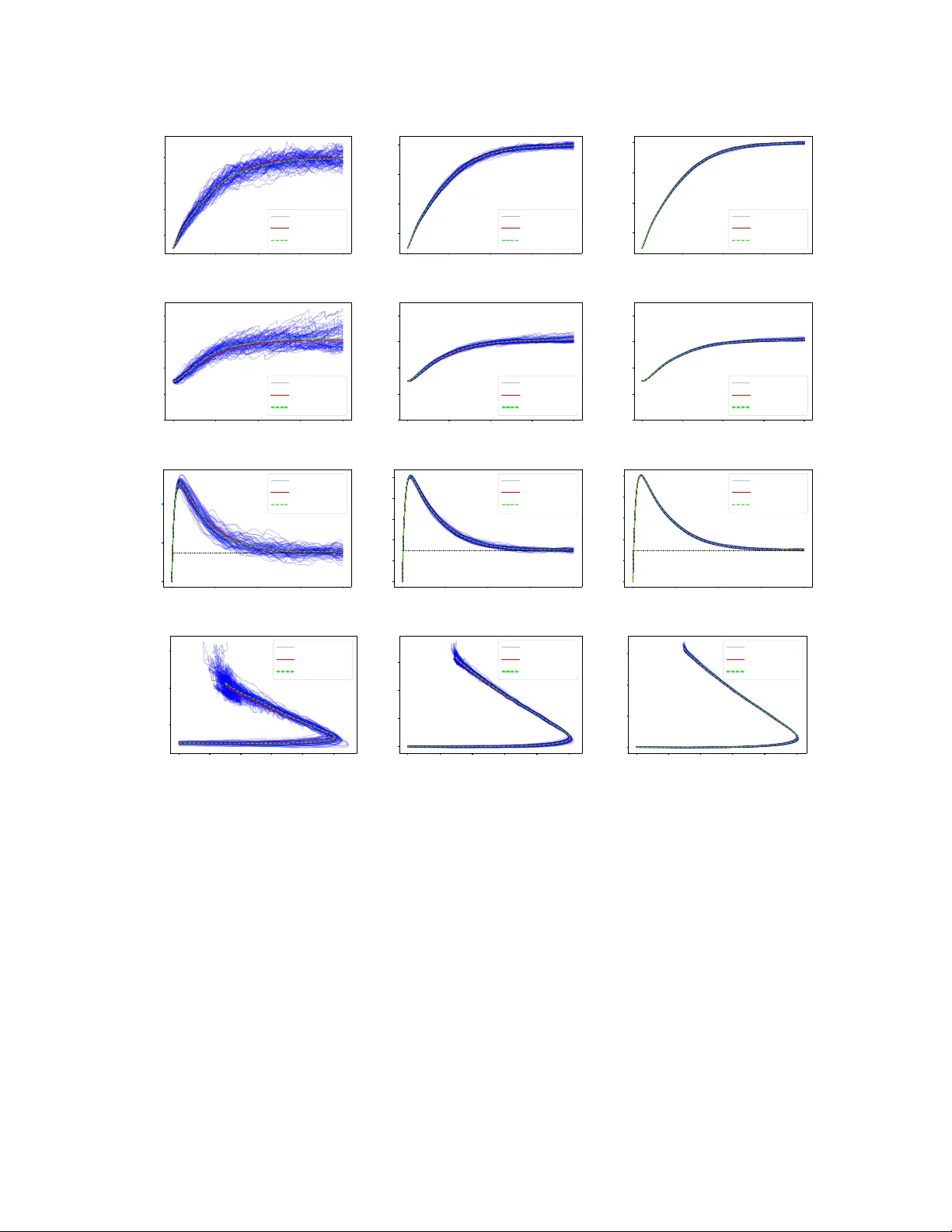
Individual-based sto c hastic mo del with un b ounded gro wth, birth and death rates: a tigh tness result Virgile Bro du ∗ Marc h 24, 2026 Abstract W e study population dynamics through a general growth/degro wth-fragmentation process, with resource consumption and un b ounded gro wth/degrowth, birth and death rates. Our model is structured in a p ositiv e trait called ener gy (whic h is a proxy for any biological parameter such as size, age, mass, protein quantit y ...), and the jump rates of the pro cess can b e arbitrarily high dep ending on individual energies, which has not been considered yet in the literature. After a preliminary study to construct well-deﬁned ob jects (which is necessary contrary to similar works, b ecause of the explosion of individual rates), we consider a classical sequence of renormalizations of the underlying process and obtain a tigh tness result for the associated laws in large-p opulation asymptotics. W e characterize the accumulation points of this sequence as solutions of an integro- diﬀeren tial system of equations, which prov es the existence of measure solutions to this system. F urthermore, if such a measure solution is unique, then our tigh tness result b ecomes a conv ergence result to wards this unique process. W e illustrate our w ork with the case of al lometric rates ( i.e. they are assumed to b e p o wer functions) and even tually present numerical simulations in this allometric setting. Keyw ords: individual-based mo del, Jumping Marko v Pro cess, large-p opulation asymptotics, martin- gale problem, measure-v alued pro cess, tightness, un b ounded jump rates. 1 In tro duction W e prop ose a general framework to study a p opulation, with comp etition b et ween individuals through resource consumption, and design a sto c hastic individual-based mo del. W e gather all individual tra- jectories into a measure-v alued p opulation pro cess. This work is in line with a rich literature ab out similar individual-based mo dels, originating with [ FM04 ], follow ed b y [ CFM08 ] with m utations, adding an age structure in [ T ra08 ], an interaction with resources in [ CF15 ], and a diﬀusion term in [ Tch24 ]. The main con tribution of all these pap ers is a con vergence result in large-population asymptotics, for a suitable renormalization of the underlying sto c hastic pro cesses, tow ards the solution µ ∗ to an in tegro- diﬀeren tial system of equations, which is deterministic conditionally to the initial condition (see the original Theorem 5.3. in [ FM04 ], or the recent Theorem 2.1. and Theorem 3.2. in [ Tch24 ]). The main result of our article is Theorem 4.1 , which is a tightness result similar to these con vergences established in the literature. One common feature b et ween previous pap ers is that growth, birth and death rates are b ounded, and µ ∗ in tegrates b ounded functions. Our work go es b ey ond these previous results for the following reasons. First, our jump rates are not necessarily b ounded, which adds p oten tial prob- lems of explosion of individual energy or p opulation size in ﬁnite time, and technical diﬃculties in the pro ofs, but allows more general and biologically relev ant mo dels. W e develop the case of al lometric scalings ( i.e. the jump rates are p ow er functions), which seem to b e a key ingredient for mo delling the b eha vior of sp ecies [ P et86 , BGA + 04 , MM19 , BBCF25 ], in Section 5 . Then, an y accumulation p oin t, ∗ Universit ´ e de Lorraine, Inria, IECL, F-54000 Nancy , F rance 1 still denoted as µ ∗ , integrates a broader set of functions, not necessarily b ounded (see Lemma 6.2 ). Hence, our w ork could b e adapted to generalize existing results on growth-fragmen tation mo dels such as [ T ra08 ] or [ CF15 ]. W e make a sp eciﬁc c hoice for the fragmentation modelling: ev ery oﬀspring in the p opulation ap- p ears with energy x 0 > 0, which is a ﬁxed parameter of the mo del. The introduction of this parameter is link ed to the biological motiv ation of this work, presented in [ BBCF25 ], where w e make x 0 v ary to obtain necessary conditions for our mo del to b e biologically relev an t with allometric functional param- eters. On the contrary , in the present article, x 0 is ﬁxed once and for all. Our work could certainly b e extended to other v arious fragmentation patterns, like binary ﬁssion [ DHKR15 ], conserv ative and symmetrical division k ernels [ CCF16 ], or self-similar splitting densities [ L W07 ]. Individual tra jectories dep end on the evolution of the resource o ver time, which in turn dep ends on individual energies. Th us, we study a pro cess ( µ t , R t ) t ≥ 0 , where µ is a ﬁnite p oint measure rep- resen ting the state of the p opulation, and R ∈ [0 , R max ] the amoun t of resources ( R max > 0 b eing a parameter of the mo del). This measure-v alued pro cess is constructed with Poisson p oin t measures and is piecewise deterministic. Compared to other existing mo dels [ T ra08 , CF15 ], due to the choice of unbounded jump rates in our case, additional work is necessary to ensure that the pro cess is well deﬁned for every t ≥ 0. Then, we introduce a sequence of renormalized pro cesses ( µ K t , R K t ) t ≥ 0 con- structed with the same pro cedure. The parameter K is a scaling parameter representing the n umber of individuals in the p opulation at time 0. W e w ant to understand the b eha vior of our mo del in a large p opulation asymptotic, when the parameter K go es to + ∞ . Imp ortan tly , unlike previous work on similar renormalizations of individual-based mo dels [ FM04 , CFM08 , T ra08 , CF15 , Tch24 ], we hav e to add an additional assumption, due to the fact that our rates are un b ounded. Precisely , we assume that there exists a “Lyapuno v-type” smo oth and non-decreasing function ω , asso ciated with the func- tional parameters of the mo del (see the up coming ( H2 ) in Theorem 1.1 ). This will allo w us to control sto c hastic integrals asso ciated to our renormalized pro cesses, and hav e tw o imp ortan t consequences. First, we can prov e martingale prop erties for our pro cesses (see Prop osition 3.3 ), which is a key in- gredien t of the pro of in Section 6 . Then, we can control the expectation of the population size at any time uniformly on K (see Prop osition 3.4 ). Pro vided that such a function ω exists, we endo w the set of measures integrating the function ω with a weigh ted top ology whic h is not standard. W e call it the ω -w eak top ology , and write ( M ω ( R ∗ + ) , w) for the asso ciated top ological space (see Section 4 and App endix B.2 in [ Bro25 ] for details). Let us give immediately a taste of our main result with as least tec hnical details as p ossible. In the following, b ( x ) is the birth rate for an individual with energy x , and similarly d ( x ) is the death rate. The functions b and d are non-negative. The function g : ( x, R ) 7→ g ( x, R ) accounts for the in- stan taneous rate of growth or degrowth for an individual with energy x and resources R . The function ρ : ( R , µ ) 7→ ρ ( R, µ ) is the instantaneous rate of increase or decrease of resources R consumed b y the p opulation µ . The functions g and ρ can change sign, dep ending on the resources R and the state of the individual/p opulation. F or more details ab out the previous functional parameters, we refer the reader to Section 2.1 . In the follo wing, we write ⟨ µ, φ ⟩ := Z R ∗ + φ ( x )d µ ( x ) for every µ ∈ M ω ( R ∗ + ) and φ measurable. A simpliﬁed summarization of our tigh tness result reads as follo w: Theorem 1.1. First, we assume that ( H0 ) ∀ x > 0 , g ( x, 0) < 0 < g ( x, R max ) , ( H1 ) ∀ x > 0 , Z x 0 d ( t ) g ( t, 0) d t = −∞ . Then, we assume that ther e exists a weight function ω such that 2 ( H2 ) ω ∈ C 1 ( R ∗ + ) is p ositive, non-de cr e asing, Lipschitz c ontinuous on (1 , + ∞ ) , and ( a ) ∃ c g > 0 , ∀ x > 0 , sup R ∈ [0 ,R max ] | g ( x, R ) | ≤ c g ω ( x ) , ( b ) ∃ c b > 0 , ∀ x > 1 , b ( x ) ≤ c b ω ( x ) , ( c ) ∃ c d > 0 , ∀ x > 0 , d ( x ) ω ( x ) ≤ c d . Final ly, we assume that the se quenc e   µ K t , R K t  t ≥ 0  K ∈ N ∗ of r enormalize d pr o c esses (formal ly deﬁne d in Se ction 3 ) is such that ( H3 ) ther e exists a r andom variable µ ∗ 0 ∈ M ω ( R ∗ + ) such that ( µ K 0 ) K ∈ N ∗ c onver ges in law towar ds µ ∗ 0 in ( M ω ( R ∗ + ) , w) , ( H4 ) ther e exists p > 1 such that sup K ∈ N ∗ E   µ K 0 , 1 + Id + ω  p  < + ∞ . Under ( H0 ) , ( H1 ) , ( H2 ) , ( H3 ) , ( H4 ) , for al l T ≥ 0 , the se quenc e   µ K t , R K t  t ∈ [0 ,T ]  K ∈ N ∗ is tight in the Skor okho d sp ac e D ([0 , T ] , ( M ω ( R ∗ + ) , w) × [0 , R max ]) . A ny of its ac cumulation p oint ( µ ∗ t , R ∗ t ) t ∈ [0 ,T ] is a c ontinuous pr o c ess and veriﬁes almost sur ely, for al l t ∈ [0 , T ] , R ∗ t = R ∗ 0 + Z t 0 ρ ( R ∗ s , µ ∗ s )d s, (1) and for every φ : ( t, x ) 7→ φ ( t, x ) =: φ t ( x ) smo oth enough and dominate d by ω , ⟨ µ ∗ t , φ t ⟩ = ⟨ µ ∗ 0 , φ 0 ⟩ + Z t 0 Z R ∗ +  ∂ 1 φ ( s, x ) + g ( x, R ∗ s ) ∂ 2 φ ( s, x ) + b ( x )( φ s ( x 0 ) + φ s ( x − x 0 ) − φ s ( x )) − d ( x ) φ s ( x )  µ ∗ s (d x )d s, (2) wher e ∂ 1 , r esp e ctively ∂ 2 , ar e the p artial derivatives with r esp e ct to the ﬁrst, r esp e ctively se c ond, vari- able. Assumptions ( H0 ) and ( H1 ) are part of the mo del, and necessary for the go od deﬁnition of individual tra jectories (see Section 2.3 ). Then, Assumption ( H2 ) is necess ary to obtain martingale prop erties for our pro cesses (see Section 3.2 ). Note that the case of b ounded rates is included in Theorem 1.1 , simply b y choosing ω ≡ 1. Finally , Assumptions ( H3 ) and ( H4 ) are classical assumptions to prov e this kind of tightness result (see the original Assumption C1.1 in [ FM04 ], or Assumption 4 in [ T ra08 ]), but adapted here to our setting with the weigh t function ω . Our main result, which is Theorem 4.1 in Section 4 , will b e stronger than Theorem 1.1 , b ecause it relies on weak er, though more complex, assumptions on the weigh t function ω . Assumption ( H2 ) will thus replaced by the combination of Assumption 2.9 and Assumption 4.1 . Note that the limiting system ( 1 )-( 2 ) is very similar to those obtained in previous works (see for example Theorem 5.2 in [ CF15 ]), but with tw o main diﬀerences. First, Equation ( 2 ) is not only v alid for b ounded functions, but for functions dominated by ω , whic h can be un b ounded (see Figure 1 ). Then, the term m ultiplied b y b ( x ) in Equation ( 2 ) can b e in terpreted as a birth term, and is naturally adapted to our sp eciﬁc fragmen tation mo delling with parameter x 0 . T o the b est of our knowledge, this is the ﬁrst tightness result with un b ounded rates for this kind of individual-based mo del. The sketc h of the pro of follows the pro cedure initially prop osed b y F ournier and M´ el ´ eard [ FM04 ], but at each step, w e encounter additional diﬃculties due to the interaction with the resource and unbounded rates. In particular, w e extend results of Ro elly [ Ro e86 ] in Theorem 6.1 , and M ´ el´ eard-Ro elly [ MR93 ] in Theorem 6.2 to w ork with the ω -w eak top ology . 3 In Section 2.1 and 2.2 , w e construct the process ( µ t , R t ) t . In Section 2.3 and 2.4 , w e provide as- sumptions under which this process is w ell-deﬁned for every t ≥ 0. W e also in tro duce the w eight function ω . In Section 2.5 , we show martingale prop erties of the pro cess. In Section 3 , we introduce the sequence of renormalized pro cesses ( µ K t , R K t ) t ∈ [0 ,T ] . W e present our main result in Theorem 4.1 of Section 4 , along with p ossible extensions of this result and conjectures in Section 4.2 . In particular, if there exists a unique solution to the system ( 1 )-( 2 ), then our tightness result b ecomes a conv ergence result. The uniqueness of the limiting pro cess in the case of b ounded rates is well-kno wn (see Prop o- sition I I.5.7. in [ Bro25 ]). It remains an op en question to know if w e can tackle more general cases with unbounded rates, and we provide some directions of researc h in Section 4.2.1 . In Section 5 , we illustrate our results, b oth theoretically and numerically , with p o wer functions for the jump rates. As far as individual-based mo dels are concerned, this so-called al lometric setting has not b een studied yet, except for our previous mo del with constan t resources in [ BBCF25 ]. Finally , the pro of of Theorem 4.1 is dev elop ed in Section 6 . In App endix A , we provide the pro ofs of intermediate results, including Theorem 6.1 and Theorem 6.2 ; and in App endix B , we giv e our simulation parameters and algorithms for Section 5 . Note that we will also refer extensiv ely to [ Bro25 ] for tec hnical, but classical details. 2 Deﬁnitions and assumptions First, in Section 2.1 , we deﬁne individual dynamics, i.e. deterministic metab olism and resource con- sumption, and random birth or death ev ents. Then, in Section 2.2 , w e in tro duce notations to gather all the individual ﬂo ws and resource dynamics in to one deterministic ﬂow b et ween random jumps. Then, w e provide an algorithmic construction of the process ( µ t , R t ) t with P oisson p oin t measures, v alid up to a stopping time accounting for tw o p ossible problematic ev ents. The ﬁrst one is the p ossibilit y for individual tra jectories to reac h 0 or + ∞ in ﬁnite time b et ween random jumps, and the second one is the p ossible accumulation of jump times at the p opulation level. In Section 2.3 , we pro vide an as- sumption to address the ﬁrst problematic even t. Then, in Section 2.4 , we resolve the second problem, b y giving a general setting under which the population pro cess is almost surely well-deﬁned for t ∈ R + . Once this is done, in Section 2.5 , w e show martingale prop erties for the pro cess ( µ t , R t ) t ≥ 0 . 2.1 Individual and resource dynamics In this section, w e in tro duce the functional parameters and main mechanisms of our mo del at the individual level, but note that the formal construction of the p opulation pro cess is done in Section 2.2 . T o distinguish b etw e en individuals, we deﬁne the set of indices as U := [ n ∈ N ( N ∗ ) n +1 . Ov er time, every individual in the p opulation will ha ve an index of the form u := u 1 ...u n +1 with some n ≥ 0, and some p ositiv e integers u 1 , ..., u n . A t time t ≥ 0, an aliv e individual indexed by u in the p opulation is c haracterized b y a trait called ener gy and written ξ u t ∈ R ∗ + ∪ { ∂ } , where ∂ is a cemetery state. Ev ery individual comp ete for a ﬂuctuating sto c k of resources R t ∈ R + , can die and reac h the cemetery state ∂ , and can repro duce several times during its life. When a birth o ccurs, w e add an individual to the p opulation, with a new index in U . In the p opulation, at time t ≥ 0, we denote as V t the set of alive individuals at this time ( i.e. whose energy is not ∂ at time t ). Ev ery alive individual u ∈ V t is represented by a Dirac mass at ξ u t . Thus, we will deﬁne the population pro cess µ t as a point measure giv en at time t b y µ t := X u ∈ V t δ ξ u t . (3) 4 An individual tra jectory is deterministic betw een some random jump times, corresponding to birth or death ev ents. Birth F or t ≥ 0, an individual indexed by u ∈ V t − with energy ξ u t − ∈ R ∗ + giv es birth to a single oﬀ- spring at rate b ( ξ u t − ). This individual transfers a constant amount of energy x 0 to the oﬀspring. The energy of the individual go es from ξ u t − to ξ u t := ξ u t − − x 0 . The p oin t measure then jumps to µ t := µ t − − δ ξ u t − + δ ξ u t − − x 0 + δ x 0 . If the parent has the lab el u := u 1 ...u n and this is the k -th birth jump for this paren t for k ≥ 1, the index of the oﬀspring is uk := u 1 ...u n k . Then, we set V t := V t − ∪ { uk } . ξ u t − x 0 ξ u t − − x 0 W e assume that the birth rate b is equal to 0 for every x ≤ x 0 , so that no individual with negative energy appears during a birth even t. Also, we assume that b is non-negative and con tinuous for x > x 0 . Death F or t ≥ 0, an individual indexed by u ∈ V t − with energy ξ u t − ∈ R ∗ + dies at p ositiv e and con tinu- ous rate d ( ξ u t − ). Then, the individual pro cess jumps to ξ u t := ∂ and we set ξ u s := ∂ for every s ≥ t . The point measure jumps to µ t := µ t − − δ ξ u t − , and w e set V t := V t − \ { u } . Energy loss and resource consumption 1. F or t ≥ 0, an individual u ∈ V t with energy ξ u t ∈ R ∗ + loses energy o ver time, at non-negative and C 1 ( R ∗ + ) rate ℓ ( ξ u t ). W e are interested in situations where ℓ is a p ositiv e function ( i.e. w e consider a true growth/degro wth-fragmentation mo del with p ossibly decreasing energies ov er time) to mo del the metab olic rate of individuals [ BGA + 04 , BBCF25 ]. Ho wev er, note that we also allow ℓ ≡ 0, so that our mo del can b e adapted to generalize previous growth-fragmen tation mo dels where individual traits are only increasing [ T ra08 , CF15 ]. 2. In order to balance this energy loss, this individual consumes the resource at rate f ( ξ u t , R t ). Imp ortan tly , we supp ose that f is of the form f ( ξ , R ) := ϕ ( R ) ψ ( ξ ) , where ψ is a C 1 ( R ∗ + ) p ositive function. Also, we assume that ϕ is a C 1 ( R + ) non-decreasing function on R + , verifying ϕ (0) = 0 and lim x → + ∞ ϕ ( x ) = 1. Finally , w e suppose that ϕ is Lipschitz contin uous on R + , meaning that ∃ k > 0 , ∀ R 1 , R 2 ≥ 0 , ∀ x > 0 , | f ( x, R 1 ) − f ( x, R 2 ) | ≤ k | R 1 − R 2 | ψ ( x ) . (4) Th us, b et ween t wo random jump times (due to birth or death even ts), the energy evolv es according to the follo wing equation: d ξ u t d t = f ( ξ u t , R t ) − ℓ ( ξ u t ) =: g ( ξ u t , R t ) . (5) Remark that g : ( x, R ) 7→ g ( x, R ) is C 1 , 1 ( R ∗ + × R + ), meaning that it is diﬀerentiable with contin uous deriv atives in b oth its v ariables. Also, one can replace f b y g in ( 4 ). It is p ossible that at some time t ≥ 0, ξ u t reac hes either 0 or + ∞ (v anishing energy or explosion of ( 5 ) in ﬁnite time b efore a jump ev ent). W e will make assumptions in Section 2.3 to av oid this situation almost surely . F or now, if this happ ens at some time t , we adopt the conv en tion ξ w s := ∂ for every s ≥ t and w ∈ V t − . Also, 5 w e set the p oin t measure to µ s := 0 for all s ≥ t , and V s := ∅ for s ≥ t . Finally , for any t ≥ 0 and u ∈ U , if u / ∈ V t , w e set ξ u t := ∂ (in particular, individuals that are not born yet at time t ha ve energy ∂ ). Resource dynamics Let χ > 1, R max > 0 and ς ∈ C 1 ( R + ), such that ς (0) ≥ 0 and ς ( R ) < 0 if R ≥ R max . Betw een random jumps, the quantit y of resource R t ∈ R + satisﬁes the follo wing equation d R t d t = ρ ( µ t , R t ) := ς ( R t ) − χ Z R ∗ + f ( x, R t ) µ t (d x ) . (6) The function ρ is w ell-deﬁned on M P ( R ∗ + ) × R + , where M P ( R ∗ + ) is the space of ﬁnite p oin t measures on R ∗ + . Equation ( 6 ) means that in the absence of individuals in the population, the amoun t of resource ev entually stabilizes at some R eq ∈ [0 , R max ]. F or the renewal function ς , one can think for example of a logistic gro wth R ≥ 0 7→ R ( R eq − R ) with R eq ≤ R max . This is a classical assumption in literature for biotic resources [ BLLD11 , YKR18 , FBC21 ]. Another example is the case of a chemostat, where we can tak e ς : R ≥ 0 7→ D ( R in − R ), with a dilution rate D > 0, and the constant R in ≤ R max can b e in terpreted as an abiotic nutrien t ﬂow in the c hemostat [ CF15 ]. The co eﬃcien t χ can b e interpreted as the in verse of the conv ersion eﬃciency . The ratio 1 /χ < 1 represen ts the prop ortion of resource consumed by individuals eﬀectively conv erted to energy . W e supp ose that χ is a cons tan t, which is a usual assumption in literature [ LL05 ], even if in [ FBC21 ], the authors make χ dep end on individual energy ov er time. The in tegral quantit y represents the speed at whic h the whole p opulation consumes the resource at time t . This non-linear term is an indirect source of comp etition b et ween individuals. If we choose an initial condition R 0 ∈ [0 , R max ], Equation ( 6 ) enforces that R t ∈ [0 , R max ] for ev- ery t ≥ 0, as long as Z R ∗ + ψ ( x ) µ t (d x ) < + ∞ (in particular, this is the case if µ t ∈ M P ( R ∗ + )). Moreov er, if R 0 > R max , even with no individuals in the p opulation, the resource will decrease to R max . Hence, without loss of generality , we assume that R 0 ∈ [0 , R max ]. Also, we make the following assumption. Assumption 2.1. ∀ x > 0 g ( x, R max ) > 0 . If Assumption 2.1 is not veriﬁed, as ϕ is non-decreasing, w e obtain ∃ M > 0 , ∀ x ≤ M , ∀ R ∈ [0 , R max ] g ( x, R ) ≤ 0 . Considering ( 5 ), this means that if the initial energy of an individual is in (0 , M ], then it will remain in this compact set ov er time. In other terms, if Assumption 2.1 is not v eriﬁed, we impose an a priori upp er b ound on the maximal energy in our mo del. Similar mass-structured mo dels where the maximal mass M of an individual is deterministically b ounded are already developed in previous works [ CF15 , CCF16 ]. Although observed living sp ecies ob viously hav e b ounded masses, w e wan t to design a mo del where this b ound is not artiﬁcially imp osed by the mo del, but results from interaction with a limiting resource. This is why in our setting, we allow individual energies to increase indeﬁnitely , at least if there are suﬃcient resources ( i.e. with R max resources are av ailable), whic h is expressed in Assumption 2.1 . In all the rest of this article, we implicitly w ork under Assumption 2.1 . Note that if ℓ is a p ositive function, Assumption 2.1 corresponds to Assumption ( H0 ) in Theorem 1.1 . Lemma 2.2. Assumption 2.1 implies that ϕ ( R max ) > 0 and ∀ x > 0 , ψ ( x ) > ℓ ( x ) . Pr o of . This is straightforw ard from our assumptions on ψ , ϕ and ℓ . 6 2.2 Algorithmic construction of the pro cess with Poisson p oin t measures 2.2.1 Deterministic ﬂow b et w een random jumps W e begin with the deﬁnition of the deterministic ﬂo w asso ciated to individual energies and the amount of resources b etw een random jumps. W e pro vide U with the lexicographical order, denoted as ≺ , and consider a ﬁnite subset V ⊆ U of cardinality | V | ∈ N . It means that there exists u 1 ≺ ... ≺ u | V | elemen ts of U , such that V = { u 1 , ..., u | V | } , with V = ∅ if | V | = 0. Let us ﬁx an initial condition R 0 ∈ [0 , R max ] and ( ξ u j 0 ) 1 ≤ j ≤| V | ∈  R ∗ +  | V | individual energies indexed by V . In the following, we will ligh ten this notation in to Ξ 0 := ( ξ u 0 ) u ∈ V . W e write  ( X u t (Ξ 0 , R 0 )) u ∈ V , X ℜ t (Ξ 0 , R 0 )  for a solution to the system of | V | + 1 coupled equations d X ℜ t (Ξ 0 , R 0 ) d t = ρ X u ∈ V δ X u t (Ξ 0 ,R 0 ) , X ℜ t (Ξ 0 , R 0 ) ! , (7) d X u t (Ξ 0 , R 0 ) d t = g ( X u t (Ξ 0 , R 0 ) , X ℜ t (Ξ 0 , R 0 )) for u ∈ V , (8) with initial condition at time 0 X ℜ 0 (Ξ 0 , R 0 ) = R 0 , X u 0 (Ξ 0 , R 0 ) = ξ u 0 for u ∈ V . Prop osition 2.3. L et V ⊆ U b e ﬁnite and (( ξ u 0 ) u ∈ V , R 0 ) ∈ ( R ∗ + ) | V | × [0 , R max ] . Then, ther e exists a neighb orho o d O ⊆ ( R ∗ + ) | V | × [0 , R max ] of (( ξ u 0 ) u ∈ V , R 0 ) , and a neighb orho o d J ⊆ R + of 0, such that 1. F or every (( ξ u ) u ∈ V , R ) ∈ O , ther e exists a unique lo c al solution with values in ( R ∗ + ) | V | × [0 , R max ] to the system of c ouple d e quations ( 7 ) - ( 8 ) , starting fr om (( ξ u ) u ∈ V , R ) at time 0. This solution is at le ast deﬁne d on J , and denote d as  ( X u t (Ξ , R )) u ∈ V , X ℜ t (Ξ , R )  , with Ξ := ( ξ u ) u ∈ V . 2. The function ( t, ( ξ u ) u ∈ V , R ) ∈ J × O 7→  ( X u t (Ξ , R )) u ∈ V , X ℜ t (Ξ , R )  is C 1 , 1 ( J × O ) , and C 2 in the variable t . Pr o of . As ς ∈ C 1 ( R + ), and f , g are C 1 , 1 ( R ∗ + × R + ), classical arguments entails the result (see Corollaire I I.2. and Th´ eor ` eme I I.10. in Chapter X of [ ZQ96 ]). Remark: The previous ob jects do not dep end on the set of indices V . W e use these notations to b e able to identify any individual b y an index and keep track of its energy ov er time, in the up coming construction of our p opulation pro cess. W e in tro duce t exp (Ξ 0 , R 0 ) ∈ (0 , + ∞ ] the maximal time of existence of the solution to ( 7 )-( 8 ) starting from (Ξ 0 , R 0 ) at time 0 highlighted in Prop osition 2.3 . The deterministic time t exp (Ξ 0 , R 0 ) is ﬁnite, if and only if one of the X u t (Ξ 0 , R 0 ) reaches 0 or + ∞ in ﬁnite time. Finally , we deﬁne a ﬂo w X with a measure-v alued ﬁrst comp onen t, to b e able to use it in the up coming deﬁnition of the sto c hastic measure-v alued pro cess ( µ t , R t ) t . Suppose that µ 0 ∈ M P ( R ∗ + ) is suc h that µ 0 = X u ∈ V δ ξ u 0 , with µ 0 = 0 if V = ∅ . Then, in the following, we write t exp ( µ 0 , R 0 ) := t exp (Ξ 0 , R 0 ), and this do es not dep end on the set of indices V . Also, for t ∈ [0 , t exp ( µ 0 , R 0 )), w e deﬁne X t ( µ 0 , R 0 ) :=  P u ∈ V δ X u t (Ξ 0 ,R 0 ) , X ℜ t (Ξ 0 , R 0 )  , 7 and this again do es not dep end on the indexing by V . Finally , we adopt the conv ention X t ( µ 0 , R 0 ) := (0 , 0) for every t ≥ t exp ( µ 0 , R 0 ). W e thus ha ve deﬁned the deterministic ﬂow with measure-v alued ﬁrst comp onen t X : M P ( R ∗ + ) × R + × R + → M P ( R ∗ + ) × R + ( µ, R, t ) 7→ X t ( µ, R ) . In the follo wing, for µ measure on R ∗ + and f measurable from R ∗ + to R , w e write ⟨ µ, f ⟩ := Z R ∗ + f d µ. 2.2.2 Algorithmic construction of the pro cess First, we deﬁne individual energies (( ξ u t ) u ∈U ) t , the set of alive individuals ( V t ) t and the amount of resources ( R t ) t inductiv ely , by constructing a sequence of successive random jump times ( J n ) n ≥ 0 , b et w een which the dynamics are deterministic (note immediately that our construction will then b e v alid only up to time sup n ∈ N J n ). Then, we gather individual pro cesses into a measure-v alued pro- cess ( µ t ) t . Betw een tw o jump times, the pro cess ( µ t , R t ) t will b e deterministic and will follo w the ﬂo w with measure-v alued ﬁrst comp onen t X deﬁned in Section 2.2.1 . W e consider N (d s, d u, d h ) and N ′ (d s, d u, d h ) tw o independent Poisson point measures on R + × U × R ∗ + , with in tensity d s × n (d u ) × d h , with n (d u ) := P w ∈U δ w (d u ). The supp ort of N , resp ectiv ely N ′ , on R + × U × R ∗ + is a count- able random set, denoted as supp( N ), resp ectiv ely supp( N ′ ). This is a random v ariable v erifying N (d s, d u, d h ) = P ( s,u,h ) ∈ supp( N ) δ ( s,u,h ) , respectively the same equation with N ′ . F or the initial condition, let ( µ 0 , R 0 ) b e a random v ariable taking v alues in M P ( R ∗ + ) × [0 , R max ]. W e deﬁne N 0 := ⟨ µ 0 , 1 ⟩ the initial num b er of individuals, V 0 := { 1 , ..., N 0 } ⊆ U , and Ξ 0 := ( ξ u 0 ) u ∈ V 0 the initial individual energies. Thus, w e index alive individuals at time 0 so that µ 0 := P u ∈ V 0 δ ξ u 0 . Also, for u / ∈ V 0 , we set ξ u 0 := ∂ . The Poisson p oint measures N and N ′ are independent from ( µ 0 , R 0 ). The canonical ﬁltration asso ciated to ( µ 0 , R 0 ), N and N ′ is ( F t ) t ≥ 0 . W e now deﬁne the sequence ( J n ) n ∈ N of successive jump times of the p opulation pro cess. First, we set J 0 := 0, and then supp ose that our pro cess is describ ed until some time J n < + ∞ with n ≥ 0. A t time J n , there exists a ﬁnite V J n ⊆ U , asso ciated to individual energies Ξ J n := ( ξ u J n ) u ∈ V J n . With the con ven tion inf ( ∅ ) = + ∞ , w e deﬁne J b n +1 := inf { t ∈ ( J n , J n + t exp (Ξ J n , R J n )) , ( t, u, h ) ∈ supp( N ) , u ∈ V J n , h ≤ b  X u t − J n (Ξ J n , R J n )  } , J d n +1 := inf { t ∈ ( J n , J n + t exp (Ξ J n , R J n )) , ( t, u, h ) ∈ supp( N ′ ) , u ∈ V J n , h ≤ d  X u t − J n (Ξ J n , R J n )  } . First if J n + t exp (Ξ J n , R J n ) = J b n +1 ∧ J d n +1 = + ∞ , it means that there are no jumps anymore, and no explosion of the solution to ( 7 )-( 8 ) starting from (Ξ J n , R J n ). Then, we set J n +1 = + ∞ , and for t ≥ J n , V t = V J n . Concerning individual energies, for t ≥ J n , if u / ∈ V J n , then ξ u t = ∂ , and  ( ξ u t ) u ∈ V J n , R t  =  ( X u t − J n (Ξ J n , R J n )) u ∈ V J n , X ℜ t − J n (Ξ J n , R J n )  . Else if J n + t exp (Ξ J n , R J n ) < J b n +1 ∧ J d n +1 = + ∞ , it means that one or several individual energies reac h 0 or + ∞ at time J n + t exp (Ξ J n , R J n ) (which is an ev ent that w e will av oid almost surely in Section 2.3 ). Then, w e set J n +1 = J n + t exp (Ξ J n , R J n ), and for t ∈ ( J n , J n +1 ), w e set V t = V J n and if u / ∈ V J n , then ξ u t = ∂ . In addition, for t ∈ ( J n , J n +1 ), w e set  ( ξ u t ) u ∈ V J n , R t  =  ( X u t − J n (Ξ J n , R J n )) u ∈ V J n , X ℜ t − J n (Ξ J n , R J n )  . 8 Next, we set V J n +1 = ∅ , R J n +1 = R J n +1 − and for u ∈ U , ξ u J n +1 = ∂ . Remark that with these con ven tions, we necessarily get bac k to the ﬁrst case describ ed ab o ve for the deﬁnition of J n +2 (so J n +2 = + ∞ ), and ev entually obtain that for all t ≥ J n +1 , V t = ∅ and for u ∈ U , ξ u t = ∂ . Finally , if J b n +1 ∧ J d n +1 < J n + t exp (Ξ J n , R J n ), it means that one birth or death ev ent o ccurs. By prop ert y of Poisson p oin t measures, we almost surely ha ve J b n +1  = J d n +1 , and the inﬁm um in the deﬁ- nition of J b n +1 or J d n +1 is reac hed at a single elemen t ( t, u, h ) ∈ supp( N ) or supp( N ′ ). W e distinguish again betw een tw o cases. • First if J b n +1 < J d n +1 , it means that one birth even t o ccurs. This even t concerns an individual indexed b y some w ∈ V J n . Then, w e set J n +1 = J b n +1 , and for all t ∈ [ J n , J n +1 ), V t = V J n . Concerning individual energies, if u / ∈ V J n , w e set ξ u t = ∂ and  ( ξ u t ) u ∈ V J n , R t  =  ( X u t − J n (Ξ J n , R J n )) u ∈ V J n , X ℜ t − J n (Ξ J n , R J n )  . Then, at time J n +1 , a new individual app ears in the p opulation. W e set V J n +1 = V J n ∪ { w k } , where k − 1 is the num ber of oﬀspring individual w already pro duced ( i.e. the cardinality of the set { ( t, u, h ) ∈ supp( N ) , u = w , ∃ 1 ≤ m ≤ n, J b m = t } ). W e also set ξ wk J n +1 = x 0 , ξ w J n +1 = ξ w J n +1 − − x 0 and ξ u J n +1 = ξ u J n +1 − for u ∈ U \ { w , w k } . Finally , R J n +1 = R J n +1 − . • Else if J d n +1 < J b n +1 , it means that a death ev ent o ccurs. This ev ent concerns an individual indexed b y some w ∈ V J n . Then, w e set J n +1 = J d n +1 , and for all t ∈ [ J n , J n +1 ), V t = V J n . Concerning individual energies, if u / ∈ V J n , w e set ξ u t = ∂ and  ( ξ u t ) u ∈ V J n , R t  =  ( X u t − J n (Ξ J n , R J n )) u ∈ V J n , X ℜ t − J n (Ξ J n , R J n )  . Then, at time J n +1 , individual w disapp ears from the p opulation. W e set V J n +1 = V J n \ { w } . W e also set ξ w J n +1 = ∂ and ξ u J n +1 = ξ u J n +1 − for u ∈ U \ { w } . Finally , R J n +1 = R J n +1 − . By conv en tion, for all n ∈ N , J b n +1 = J d n +1 = J n +1 = + ∞ if J n = + ∞ . The sequence ( J n ) n ∈ N ∗ is non-decreasing, so we can deﬁne J ∞ := lim n → + ∞ J n . Even tually , for every t ∈ [0 , J ∞ ), we deﬁne µ t as in ( 3 ), with µ t = 0 if V t = ∅ . W e verify immediately that, if no individual energy reaches 0 or explo des, for all n ∈ N , for all t ∈ [ J n , J n +1 ), µ t coincide with the deterministic ﬂow X t − J n ( µ J n , R J n ), and is mo diﬁed at an y jump time according to the rules giv en in Section 2.1 . Note that µ t (as well as the ( ξ u t ) u ∈U , V t and R t ) is well-deﬁned only for t ∈ [0 , J ∞ ), with J ∞ p ossibly ﬁnite or inﬁnite. F or all t ∈ [0 , J ∞ ), V t is the set containing the indices of alive individuals at time t (if u / ∈ V t , then ξ u t = ∂ ; and if u ∈ V t , then ξ u t ∈ R ∗ + ). The previously describ ed update rules of the set V t at eac h jump even t mak e it adapted with resp ect to the ﬁltration ( F t ) t . In the following, we wan t to av oid almost surely the follo wing situations: Situation 1 One of the individual energy v anishes/explo des. Situation 2 There is an accum ulation of jump times. W e deﬁne τ exp := inf { J n , J n +1 = J n + t exp (Ξ J n , R J n ) < + ∞} , with the conv en tion inf ( ∅ ) = + ∞ . T o av oid Situation 1 , resp ectively Situation 2 , we need to ensure that almost surely , τ exp = + ∞ , resp ectiv ely J ∞ = + ∞ . In Section 2.3 , we give an assumption under whic h τ exp = + ∞ holds true almost surely . In Section 2.4 , we work under the assumption of Section 2.3 , and w e deﬁne a general setting under which J ∞ = + ∞ holds true almost surely . 9 2.2.3 Classical writing of the pro cess on [0 , J ∞ ∧ τ exp ) Before time τ exp , individual energies never v anish or explo de, hence the global jump rate of the p op- ulation is ﬁnite at any time in [0 , J ∞ ∧ τ exp ). Thus, for every J n < τ exp , the next jump time J n +1 is either + ∞ or a birth/death jump in the inductive construction of Section 2.2.2 . Hence, for every t ∈ [0 , J ∞ ∧ τ exp ), w e can write, with the conv ention on the ﬂow X in mind, ( µ t , R t ) = X t ( µ 0 , R 0 ) + Z t 0 Z U × R ∗ + 1 { u ∈ V s − } 1 { h ≤ b ( ξ u s − ) } [ X t − s ( µ s − + δ x 0 + δ ξ u s − − x 0 − δ ξ u s − , R s ) − X t − s ( µ s − , R s )] N (d s, d u, d h ) + Z t 0 Z U × R ∗ + 1 { u ∈ V s − } 1 { h ≤ d ( ξ u s − ) } [ X t − s ( µ s − − δ ξ u s − , R s ) − X t − s ( µ s − , R s )] N ′ (d s, d u, d h ) . This formal writing is classical in the literature (Deﬁnition 2.4. in [ T ra08 ], Section 4.1 in [ CF15 ]), and should b e understo od as a telescopic sum. First, individual energies and resources evolv e determinis- tically , following the ﬂow X t ( µ 0 , R 0 ). Then, at eac h birth or death ev ent, w e erase the current ﬂo w and replace it with a new ﬂow, mo diﬁed according to our birth and death rules. 2.3 Assumption for non v anishing/explo ding individual energies In this section, we pro vide a framew ork under which τ exp = + ∞ almost surely . Recall that this ev ent o ccurs if no individual energy reaches 0 or + ∞ in ﬁnite time. First, without further assumption, w e will sho w that interaction with limiting resources preven ts individual energies from reaching + ∞ in ﬁnite time. Then, w e will in tro duce an additional assumption to preven t individual energies from reac hing 0 in ﬁnite time (see Assumption 2.6 ). W e b egin with a classical result, asso ciated to the writing of the process in Section 2.2.3 as a telescopic sum (see for example Proposition 4.1 in [ CF15 ]), and in tro duce some notations for this purp ose. Let φ : ( t, x ) 7→ φ t ( x ) b e a C 1 , 1 ( R + × R ∗ + ) function, which means that it is diﬀerentiable with con tin uous deriv atives in both its v ariables. Recall that w e write ∂ 1 φ , resp ectiv ely ∂ 2 φ , for the ﬁrst, respectively second partial deriv ative, and also for ev ery t ≥ 0 w e deﬁne Φ t : ( R, x ) ∈ R + × R ∗ + 7→ ∂ 1 φ ( t, x ) + g ( x, R ) ∂ 2 φ ( t, x ) . (9) Note that Φ dep ends on φ , but to ligh ten the notations, we c ho ose to write it this w ay in all the rest of this article. The notation Φ will alwa ys b e related to the deﬁnition in ( 9 ) with a function φ w e work with without am biguity . Lemma 2.4. L et φ ∈ C 1 , 1 ( R + × R ∗ + ) , and F ∈ C 1 , 1 ([0 , R max ] × R ) . The pr o c ess deﬁne d in Se ction 2.2.2 10 veriﬁes that, for al l t ∈ [0 , J ∞ ∧ τ exp ) , F ( R t , ⟨ µ t , φ t ⟩ ) = F ( R 0 , ⟨ µ 0 , φ 0 ⟩ ) + Z t 0  ρ ( µ s , R s ) ∂ 1 F ( R s , ⟨ µ s , φ s ⟩ ) + ⟨ µ s , Φ s ( R s , . ) ⟩ ∂ 2 F ( R s , ⟨ µ s , φ s ⟩ )  d s + Z t 0 Z U × R ∗ + 1 { u ∈ V s − } 1 { h ≤ b ( ξ u s − ) }  F ( R s , ⟨ µ s − + δ x 0 + δ ξ u s − − x 0 − δ ξ u s − , φ s ⟩ ) − F ( R s , ⟨ µ s − , φ s ⟩ )  N (d s, d u, d h ) + Z t 0 Z U × R ∗ + 1 { u ∈ V s − } 1 { h ≤ d ( ξ u s − ) }  F ( R s , ⟨ µ s − − δ ξ u s − , φ s ⟩ ) − F ( R s , ⟨ µ s − , φ s ⟩ )  N ′ (d s, d u, d h ) , with Φ asso ciate d to φ as in ( 9 ) . Pr o of . This is a classical result for a pro cess written like in Section 2.2.3 , v alid pathwisely until the random time J ∞ ∧ τ exp , b ecause our pro cess is a ﬁnite v ariation pro cess (see Deﬁnition page 39 in [ Pro05 ]) with right-con tinuous sample paths on this time windo w. W e use Itˆ o’s formula (Theorem 31 page 78 in [ Pro05 ]) and a classical decomp osition of ⟨ µ t , φ t ⟩ (see for example Prop osition 4.1 in [ CF15 ]). F or a detailed proof, we refer the reader to Lemma II.1.10. in [ Bro25 ]. In the following, for t ∈ [0 , J ∞ ∧ τ exp ), we deﬁne E t := ⟨ µ t , Id ⟩ the total energy of the p opulation at time t . In the dynamics describ ed in ( 6 ), as ς is C 1 , the sp eed of renewal of R t is upp er b ounded b y || ς || ∞ , [0 ,R max ] < + ∞ , for every t ≥ 0. This resource renewal is the only income of biomass into the system described by ( µ t , R t ) t , so this shall give us a control on the total biomass of the system. Prop osition 2.5. The pr o c ess deﬁne d in Se ction 2.2.2 veriﬁes that ∀ t ∈ [0 , J ∞ ∧ τ exp ) , R t + E t ≤ R 0 + E 0 + t || ς || ∞ , [0 ,R max ] < + ∞ . (10) Pr o of . Let t ∈ [0 , J ∞ ∧ τ exp ), b y Lemma 2.4 applied to F : ( r , x ) 7→ r + x and φ : ( t, x ) 7→ x , we hav e R t + E t = R 0 + E 0 + Z t 0  ρ ( µ s , R s ) + ⟨ µ s , Φ s ( R s , . ) ⟩  d s − Z t 0 Z U × R ∗ + 1 { u ∈ V s − } 1 { h ≤ d ( ξ u s − ) } ξ u s − N ′ (d s, d u, d h ) ≤ R 0 + E 0 + Z t 0 ς ( R s )d s, whic h concludes. Note that we used in particular the fact that the constant χ in the deﬁnition ( 6 ) of ρ is larger than 1. This control of the total biomass of the system entails that individual energies almost surely do not explo de in ﬁnite time. In order to gather all our intermediate results in to the upcoming Proposition 2.7 , w e no w introduce an assumption to preven t individual energies from reaching 0 in ﬁnite time. W e adopt the con ven tion that for any x > 0, if ℓ ( x ) = 0, then d ℓ ( x ) = + ∞ . Assumption 2.6 ( Individual energy av oids 0 ) . F or al l x > 0 , Z x 0 d ℓ ( y )d y = + ∞ . 11 The only random ev ent that allo ws to a void 0 is a death, and there is no energy gain in the worst p ossible case, which is R = 0. Hence, it is natural to compare the death rate d and the energy loss ℓ in a neighborho od of 0. Assumption 2.6 expresses as an integral condition that the death rate d should dominate the energy loss ℓ near 0. Note that if ℓ is a p ositiv e function, Assumption 2.6 corresp onds to Assumption ( H1 ) in Theorem 1.1 . Prop osition 2.7. Under Assumption 2.6 , the pr o c ess deﬁne d in Se ction 2.2.2 veriﬁes ( J 1 = + ∞ ) or ( J 1 < t exp ( µ 0 , R 0 )) . The pro of of Prop osition 2.7 can b e found in App endix A.1 . W e conclude with the following corollary , using Mark ov prop ert y . Corollary 2.8. Under Assumption 2.6 , the pr o c ess deﬁne d in Se ction 2.2.2 veriﬁes τ exp = + ∞ almost sur ely. Pr o of . By deﬁnition of τ exp and construction of the process, it suﬃces to show that for every n ∈ N , w e almost surely ha ve ( J n +1 = + ∞ ) or ( J n +1 < J n + t exp ( µ J n , R J n ) < + ∞ ) . Let us ﬁx n ∈ N and work in the follo wing conditionnally to the even t { J n + t exp ( µ J n , R J n ) < + ∞} ∩ { J n +1 < + ∞} . W e aim to show that J n +1 < J n + t exp ( µ J n , R J n ) almost surely . W e deﬁne ( ˜ µ 0 , ˜ R 0 ) a random v ariable with same la w as ( µ J n , R J n ), and ( ˜ µ t , ˜ R t ) t a pro cess starting from the random initial condition ( ˜ µ 0 , ˜ R 0 ) and constructed with the algorithmic procedure described in Section 2.2.2 . The jump times with indices 0 and 1 asso ciated to ( ˜ µ t , ˜ R t ) t are naturally written ˜ J 0 and ˜ J 1 , and note that b y construction, ˜ J 0 := 0. Under the ev en t { J n +1 < + ∞} , from the strong Mark o v prop ert y for P oisson p oin t pro cesses (see Example 10.4(a) in [ DVJ07 ]), the law of J n + t exp ( µ J n , R J n ) − J n +1 conditionnally to { J n + t exp ( µ J n , R J n ) < + ∞} and F J n is equal to the la w of ˜ J 0 + t exp ( ˜ µ 0 , ˜ R 0 ) − ˜ J 1 = t exp ( ˜ µ 0 , ˜ R 0 ) − ˜ J 1 , whic h concludes thanks to Proposition 2.7 . 2.4 Assumption for a well-deﬁned p opulation pro cess ( µ t ) t for ev ery t ≥ 0 A t this step, thanks to Assumption 2.6 , we hav e τ exp = + ∞ almost surely (it is Corollary 2.8 ), and w e work under this ev ent. The pro cess ( µ t , R t ) t is still well-deﬁned only on [0 , J ∞ ), with J ∞ p ossibly ﬁnite, i.e. there is a p ossible accumulation of jump times. In Section 2.4.1 , we assume the existence of an appropriate weigh t function ω . Then, using this weigh t function, we give in Section 2.4.2 a setting under whic h almost surely , J ∞ = + ∞ . W e will even obtain in Prop osition 2.12 a stronger result, whic h implies in particular that the exp ectation of the p opulation size is ﬁnite for every t ≥ 0. 2.4.1 Deﬁnition of the w eight function ω W e deﬁne a weigh t function ω adapted to the functional parameters b , d , ϕ and ψ for t wo reasons. First, if suc h a weigh t function exists, w e shall prov e in Section 2.4.2 that ( µ t ) t is well-deﬁned on R + . Then, we will obtain in Section 2.5 imp ortan t martingale prop erties for our pro cess. W e write ℏ : x ∈ R + 7→ x + x 2 , and g : x > 0 7→ sup R ∈ [0 ,R max ] | g ( x, R ) | . Note that for x > 0, g ( x ) = max( ℓ ( x ) , ϕ ( R max ) ψ ( x ) − ℓ ( x )). Assumption 2.9 ( Existence of an appropriate w eight function ) . Ther e exists ω ∈ C 1 ( R ∗ + ) p ositive and non-de cr e asing such that • ∃ C g > 0 , ∀ x > 0 , g ( x )(1 + ω ′ ( x )) ≤ C g (1 + x + ω ( x )) , • ∃ C b > 0 , ∀ x > 0 , b ( x )(1 + ℏ ( | ω ( x 0 ) + ω ( x − x 0 ) − ω ( x ) | )) ≤ C b (1 + x + ω ( x )) , 12 • ∃ C d > 0 , ∀ x > 0 , d ( x ) ℏ ( ω ( x )) ≤ C d (1 + x + ω ( x )) . Remark: Recall that b ≡ 0 on (0 , x 0 ], so if ω is Lipschitz contin uous on (1 , + ∞ ) (whic h is equiv alent to ω ′ b ounded on (1 , + ∞ ), and en tails that x > 1 7→ ω ( x ) /x is b ounded on a neighborho od of + ∞ ), the second point of Assumption 2.9 is equiv alent to the lighter assumption ∃ C b > 0 , ∀ x > 1 , b ( x ) ≤ C b (1 + x ) . (11) Th us, we let the reader chec k that if ( H2 ) in Theorem 1.1 is v eriﬁed, then Assumption 2.9 holds true. Assumption ( H2 ) is wa y more readable, though more restrictive on ω . W e b eliev e, although it is not prov en in this pap er, that As sumption 2.9 on ω is sharp in our framework, in the sense that it is necessary and suﬃcient to obtain martingale prop erties for our pro cess with the usual techniques dev elop ed originally in [ FM04 ]. In general, pro ving the existence of a weigh t function ω verifying As- sumption 2.9 could b e a diﬃcult problem, similar to the search for Lyapuno v functions asso ciated to the extended generator of a F eller pro cess (see for example condition (CD2) in Section 4.1. of [ MT93 ], or Assumption (E) in Section 2 of [ CV23 ]). W e present in Section 5.1 an al lometric setting with unbounded functional parameters, where jump rates are pow er functions, and prov e that there exists weigh t functions ω v erifying Assumption 2.9 in this sp eciﬁc con text. It is of order x κ 1 , resp ectiv ely x κ 2 , in a neighborho o d of 0, resp ectiv ely + ∞ , with 0 ≤ κ 1 ≤ κ 2 ≤ 1. The t ypical shap e of the weigh t function ω in this setting is sho wn on Figure 1 . 0 1 2 3 4 0 1 2 3 4 ω Id Figure 1: Possible shap e of the w eight function ω with an allometric c hoice of parameters. Notice that in general, the third p oin t of Assumption 2.9 implies that dω should be bounded in a neigh b orho od of 0. Hence, if d ( x ) − − − → x → 0 + ∞ , which can be a biological assumption for the death rate d , then ω ( x ) − − − → x → 0 0 as shown on Figure 1 . W e will discuss in Section 4 how this impacts the in terpretation of the tigh tness result in Theorem 4.1 . Lemma 2.10. Assumption 2.9 is e quivalent to the c ombination of the fol lowing pr op erties. First, ω ∈ C 1 ( R ∗ + ) , is p ositive and non-de cr e asing, and then ∃ ω 1 > 0 , ∀ x > 0 , g ( x )(1 + ω ′ ( x )) + b ( x ) (1 + | ω ( x 0 ) + ω ( x − x 0 ) − ω ( x ) | ) + d ( x ) ω ( x ) ≤ ω 1 (1 + x + ω ( x )) , (12) and ∃ ω 2 > 0 , ∀ x > 0 , b ( x )( ω ( x 0 ) + ω ( x − x 0 ) − ω ( x )) 2 + d ( x ) ω 2 ( x ) ≤ ω 2 (1 + x + ω ( x )) . (13) 13 Pr o of . The fact that Assumption 2.9 implies ( 12 ) and ( 13 ) is immediate. W e can take ω 1 = C g + C b + C d and ω 2 = C b + C d . Conv ersely , if ( 12 ) and ( 13 ) hold true, we can take C g = ω 1 and C b = C d = ω 1 + ω 2 . Remark: Lemm a 2.10 giv es us an insigh t on wh y Assumption 2.9 is interesting to obtain martingale prop erties for our pro cess. Equation ( 12 ) shall provide a control for the sto c hastic integrals app earing in the decomp osition of ⟨ µ t , φ t ⟩ , using Lemma 2.4 with F : ( r, x ) 7→ x . Also, ( 13 ) is mean t to con trol the quadratic v ariation of the martingale part of these stochastic integrals (see Corollary 2.15 in Section 2.5 ). 2.4.2 Pro of of the non-accumulation of jump times F or t ∈ [0 , J ∞ ), we deﬁne N t := ⟨ µ t , 1 ⟩ . It represen ts the num b er of individuals in the p opulation at time t . W e also deﬁne Ω t := ⟨ µ t , ω ⟩ , and for M > 0, we introduce the stopping time τ M := inf { t ∈ [0 , J ∞ ) , E t + N t + Ω t ≥ M } , with the conv ention inf ( ∅ ) = + ∞ . Finally , for an y p ositiv e function w on R ∗ + , w e write φ ∈ B w ( R ∗ + ), if φ w is a bounded function on R ∗ + . Deﬁnition 2.11 ( General setting ) . In the fol lowing, we denote as ‘the gener al setting’, the fr ame- work gathering the dynamics describ e d in Se ctions 2.1 and 2.2 , Assumptions 2.6 and 2.9 , and the additional assumption E ( E 0 + N 0 + Ω 0 ) < + ∞ . W e are now ready to give the main result of this section. Prop osition 2.12. Under the gener al setting , we almost sur ely have τ M − − − − − → M → + ∞ + ∞ . (14) Then, for al l T ≥ 0 , E sup t ∈ [0 ,T ∧ J ∞ ) ( E t + N t + Ω t ) ! < + ∞ . (15) This imme diately implies that for every φ ∈ B 1+Id+ ω ( R ∗ + ) , we have E sup t ∈ [0 ,T ∧ J ∞ ) |⟨ µ t , φ ⟩| ! < + ∞ . The pro of of Prop osition 2.12 can b e found in App endix A.2 . It uses classical arguments, adapted to our general setting with the weigh t function ω . Corollary 2.13. Under the gener al setting , the pr o c ess ( µ t ) t is almost sur ely wel l-deﬁne d for every t ≥ 0 , i.e. P ( τ exp ∧ J ∞ = + ∞ ) = 1 . Pr o of . This is a direct adaptation of the pro of of p oin t (i) of Theorem 3.1 in [ FM04 ], using ( 14 ). Remark: It is p ossible to obtain the conclusion of Corollary 2.13 by replacing Assumption 2.9 with ( 11 ), using Prop osition 2.5 and classical argumen ts as in the pro of of p oint (i) in Theorem 3.1 in [ FM04 ]. One can then wonder why we work under Assumption 2.9 instead of ( 11 ), which do es not in volv e an additional w eight function ω . What makes Assumption 2.9 necessary in our work is that w e also need martingale prop erties for our pro cess (see Corollary 2.15 ) to obtain the tightness result in Theorem 4.1 . 14 2.5 Martingale prop erties In this section, w e work under the general setting , so the pro cess ( µ t , R t ) t ≥ 0 is almost surely well- deﬁned thanks to Corollary 2.13 . W e write F for the set of functions of the form F φ : ( µ, r ) ∈ M P ( R ∗ + ) × [0 , R max ] 7→ F ( r, ⟨ µ, φ ⟩ ) ∈ R , with F : ( r , x ) 7→ F ( r , x ) in C 1 , 1 ([0 , R max ] × R ) and φ ∈ C 1 ( R ∗ + ). F or such a function, we write ∂ 1 F φ ( µ, r ) := ∂ 1 F ( r , ⟨ µ, φ ⟩ ) and ∂ 2 F φ ( µ, r ) := ∂ 2 F ( r , ⟨ µ, φ ⟩ ). Finally , for F ∈ C 1 , 1 ([0 , R max ] × R ) and φ ∈ C 1 , 1 ( R + × R ∗ + ) (so that for all t ≥ 0, F φ t is w ell-deﬁned in F ), w e deﬁne M F,φ,t := F φ t ( R t , µ t ) − F φ 0 ( R 0 , µ 0 ) − Z t 0 ρ ( µ s , R s ) ∂ 1 F φ s ( R s , µ s ) + ⟨ µ s , Φ s ( R s , . ) ⟩ ∂ 2 F φ s ( R s , µ s )d s − Z t 0 Z R ∗ + b ( x )  F φ s ( R s , µ s + δ x 0 + δ x − x 0 − δ x ) − F φ s ( R s , µ s )  µ s (d x )d s − Z t 0 Z R ∗ + d ( x )  F φ s ( R s , µ s − δ x ) − F φ s ( R s , µ s )  µ s (d x )d s, (16) with Φ associated to φ as in ( 9 ). The pro cess ( M F,φ,t ) t ≥ 0 is almost surely well-deﬁned under the general setting b y Lemma 2.4 and Corollary 2.13 . In the follo wing, quadratic v ariations of square- in tegrable martingales are predictable quadratic v ariation deﬁned as in Theorem 4.2. in [ JS + 87 ]. Also, w e write e N and f N ′ for the comp ensated measures asso ciated with the Poisson p oin t measures N and N ′ ( i.e. e N (d s, d u, d h ) := N (d s, d u, d h ) − d s d u d h , and the same deﬁnition with N ′ ). Prop osition 2.14. Under the gener al setting , let F ∈ C 1 , 1 ([0 , R max ] × R ) and φ ∈ C 1 , 1 ( R + × R ∗ + ) . (i) Assume that for al l t ≥ 0 , E Z t 0 Z R ∗ + b ( x )     F φ s ( R s , µ s + δ x 0 + δ x − x 0 − δ x ) − F φ s ( R s , µ s )     µ s (d x )d s ! < + ∞ , and E Z t 0 Z R ∗ + d ( x )     F φ s ( R s , µ s − δ x ) − F φ s ( R s , µ s )     µ s (d x )d s ! < + ∞ . Then ( M F,φ,t ) t ≥ 0 is a ( F t ) t ≥ 0 -martingale. (ii) Supp ose in addition that for al l t ≥ 0 , E Z t 0 Z R ∗ + b ( x )  F φ s ( R s , µ s + δ x 0 + δ x − x 0 − δ x ) − F φ s ( R s , µ s )  2 µ s (d x )d s ! < + ∞ , and E Z t 0 Z R ∗ + d ( x )  F φ s ( R s , µ s − δ x ) − F φ s ( R s , µ s )  2 µ s (d x )d s ! < + ∞ . Then ( M F,φ,t ) t ≥ 0 is a squar e-inte gr able martingale, with pr e dictable quadr atic variation given for al l t ≥ 0 by ⟨ M F,φ ⟩ t := Z t 0 Z R ∗ + b ( x )  F φ s ( R s , µ s + δ x 0 + δ x − x 0 − δ x ) − F φ s ( R s , µ s )  2 µ s (d x )d s + Z t 0 Z R ∗ + d ( x )  F φ s ( R s , µ s − δ x ) − F φ s ( R s , µ s )  2 µ s (d x )d s 15 Pr o of . W e observe from Lemma 2.4 that M F,φ,t = Z t 0 Z U × R ∗ + 1 { u ∈ V s − } 1 { h ≤ b ( ξ u s − ) }  F ( R s , ⟨ µ s − + δ x 0 + δ ξ u s − − x 0 − δ ξ u s − , φ s ⟩ ) − F ( R s , ⟨ µ s − , φ s ⟩ )  e N (d s, d u, d h ) + Z t 0 Z U × R ∗ + 1 { u ∈ V s − } 1 { h ≤ d ( ξ u s − ) }  F ( R s , ⟨ µ s − − δ ξ u s − , φ s ⟩ ) − F ( R s , ⟨ µ s − , φ s ⟩ )  f N ′ (d s, d u, d h ) . Then, Prop osition 2.14 follows from classical results from Ikeda and W atanab e on sto c hastic integrals with respect to Poisson p oin t measures (see p.62 in [ IW14 ]). In the follo wing, we deﬁne C 1 , 1 ω ( R + × R ∗ + ) the set of functions φ ∈ C 1 , 1 ( R + × R ∗ + ) such that φ : ( t, x ) 7→ ω ( x ) or ∃ C > 0 , ∀ x > 0 , sup t ∈ R +  | φ ( t, x ) | + | ∂ 1 φ ( t, x ) | ω ( x ) 1 + x + ω ( x ) + | ∂ 2 φ ( t, x ) | ω ( x )  ≤ C ω ( x ) . Note that the function φ : ( t, x ) 7→ ω ( x ) do es not necessarily verify the previous condition (in particular, ω ′ is not necessarily b ounded). Ho wev er, we include this sp eciﬁc function in C 1 , 1 ω ( R + × R ∗ + ), b ecause w e need to b e able to apply the follo wing results to this function for the pro of of Theorem 4.1 . Corollary 2.15. Under the gener al setting , let φ ∈ C 1 , 1 ω ( R + × R ∗ + ) . Then the pr o c ess ( ⟨ µ t , φ t ⟩ ) t ≥ 0 is a semi-martingale, with for al l t ≥ 0 , a ﬁnite variation p art given by V φ,t := ⟨ µ 0 , φ 0 ⟩ + Z t 0 ⟨ µ s , Φ s ( R s , . ) ⟩ d s − Z t 0 Z R ∗ + d ( x ) φ s ( x ) µ s (d x )d s + Z t 0 Z R ∗ + b ( x )  φ s ( x 0 ) + φ s ( x − x 0 ) − φ s ( x )  µ s (d x )d s, with Φ asso ciate d to φ as in ( 9 ) , and a squar e-inte gr able martingale p art ♡ φ,t := ⟨ µ t , φ t ⟩ − V φ,t whose pr e dictable quadr atic variation is given by ⟨♡ φ ⟩ t = Z t 0 Z R ∗ + b ( x )  φ s ( x 0 ) + φ s ( x − x 0 ) − φ s ( x )  2 µ s (d x )d s + Z t 0 Z R ∗ + d ( x ) φ 2 s ( x ) µ s (d x )d s. Pr o of . W e apply Prop osition 2.14 to F : ( R , x ) ∈ [0 , R max ] × R 7→ x and φ . W e let the reader verify that w e can do so, thanks to the assumption φ ∈ C 1 , 1 ω ( R ∗ + ) (in particular, if φ  = ω , we use the fact that there exists a constant C > 0 such that | ∂ 2 φ ( t, x ) | < C for every t ≥ 0, x > 0, so | φ s ( x − x 0 ) − φ s ( x ) | ≤ C x 0 for ev ery s ∈ [0 , t ] and x > 0), Lemma 2.10 and ﬁnally Prop osition 2.12 . Remark: At this step, one can sho w that ( µ t , R t ) t ≥ 0 is a Jumping Marko v Pro cess (JMP). This particular type of F eller pro cess w as initially in tro duced by Da vis [ Dav84 ] for R n -v alued pro cesses, and called Piecewise Deterministic Mark ov Pro cesses (PDMP). Then, Jacod and Sk orokho d introduced in [ JS96 ] the general deﬁnition of a JMP , adapted to our measure-v alued setting. W e can further c haracterize the F eller pro cess ( µ t , R t ) t ≥ 0 via its extended generator (see p.45 in [ JS96 ]), and refer the reader to Proposition I I.1.20. in [ Bro25 ] for details. 16 3 Renormalization of the pro cess In this section, we w ork under Assumptions 2.6 and 2.9 . In Section 3.1 , we deﬁne a sequence   µ K t , R K t  t ≥ 0  K ∈ N ∗ , where ev ery pro cess  µ K t , R K t  t ≥ 0 is a renormalization of the initial pro cess ( µ t , R t ) t ≥ 0 deﬁned in Section 2.2 , and K is a scaling parameter representing the p opulation size at time 0, mean t to diverge to wards + ∞ . In Section 3.2 , w e use the results of Section 2 to obtain martingale and con trol prop erties for the renormalized pro cess ( µ K t , R K t ) t ≥ 0 . 3.1 Deﬁnition of the renormalized pro cess W e follo w a classical procedure, ﬁrst describ ed in [ FM04 ], and then reproduced in man y articles [ CFM08 , T ra08 , CF15 , Tc h24 ]. First, for every K ∈ N ∗ , we will deﬁne an auxiliary pro cess ( ν K t , R K t ) t ≥ 0 , follo wing the exact same construction as in Section 2.2 , but with an inv erse conv ersion eﬃciency χ K := χ/K . Thus, all the results of Section 2 will apply to ( ν K t , R K t ) t ≥ 0 , simply replacing χ with χ K . W e begin with the deﬁnition of the renormalized deterministic ﬂow follow ed by individual energies b et w een jumps. W e consider an initial condition ( ν K 0 , R 0 ) ∈ M P ( R ∗ + ) × [0 , R max ] at time 0, whic h means that there exists N ∈ N and ( ξ u,K 0 ) 1 ≤ u ≤ N in ( R ∗ + ) N suc h that ν K 0 := N X u =1 δ ξ u,K 0 , where ν K 0 = 0 if N = 0. W e write  ( X u,K t ( ν K 0 , R 0 )) 1 ≤ u ≤ N , X ℜ ,K t ( ν K 0 , R 0 )  for a solution to the system of N + 1 coupled equations d X ℜ ,K t ( ν K 0 , R 0 ) d t = ς ( X ℜ ,K t ( ν K 0 , R 0 )) − χ K Z R ∗ + f ( x, X ℜ ,K t ( ν K 0 , R 0 )) ˜ ν K t (d x ) , (17) d X u,K t ( ν K 0 , R 0 ) d t = g ( X u,K t ( ν K 0 , R 0 ) , X ℜ ,K t ( ν K 0 , R 0 )) for 1 ≤ u ≤ N , (18) where ˜ ν K t := P N i =1 δ X u,K t ( ν K 0 ,R 0 ) , and with initial condition at time 0 X ℜ ,K 0 ( ν K 0 , R 0 ) = R 0 , X u,K 0 ( ν K 0 , R 0 ) = ξ u,K 0 for 1 ≤ u ≤ N . Note that the system of equations ( 17 )-( 18 ) is similar to ( 7 )-( 8 ), where we only replace χ by χ/K . With the same arguments as in Prop osition 2.3 , we can deﬁne for t in a neighborho od of 0, denoted as [0 , t K exp ( ν K 0 , R 0 )) the renormalized ﬂow X K t ( ν K 0 , R 0 ) :=  N P u =1 δ X u,K t ( ν K 0 ,R 0 ) , X ℜ ,K t ( ν K 0 , R 0 )  , and it b eneﬁts from the same regularit y properties as X of Section 2.2 . W e also adopt the conv ention depicted in the remark after Corollary 2.8 to make sense of the previous notation for t ≥ t K exp ( ν K 0 , R 0 ). Deﬁnition 3.1 ( Renormalized pro cess ) . L et R 0 ∈ [0 , R max ] b e a r andom variable. L et ( ν K 0 ) K ≥ 1 b e a se quenc e of r andom variables in M P ( R ∗ + ) , such that sup K ≥ 1  1 K E  ⟨ ν K 0 , 1 + Id + ω ⟩   < + ∞ . (19) We use the Poisson p oint me asur es N and N ′ of Se ction 2.2 , indep endent fr om R 0 and ( ν K 0 ) K ≥ 1 . F or every K ≥ 1 , the r enormalize d pr o c ess ( µ K t , R K t ) t ≥ 0 with initial c ondition ( µ K 0 , R 0 ) , is given for every t ≥ 0 by µ K t := ν K t K and 17 ( ν K t , R K t ) = X K t ( ν K 0 , R 0 ) + Z t 0 Z U × R ∗ + 1 { u ∈ V K s − } 1 { h ≤ b ( ξ u,K s − ) } [ X K t − s ( ν K s − + δ x 0 + δ ξ u,K s − − x 0 − δ ξ u,K s − , R K s ) − X K t − s ( ν K s − , R K s )] N (d s, d u, d h ) + Z t 0 Z U × R ∗ + 1 { u ∈ V K s − } 1 { h ≤ d ( ξ u,K s − ) } [ X K t − s ( ν K s − − δ ξ u,K s − , R K s ) − X K t − s ( ν K s − , R K s )] N ′ (d s, d u, d h ) , wher e for al l t ≥ 0 , V K t is the set c ontaining alive individuals at time t , and ξ u,K t ar e individual ener gies, deﬁne d and actualize d over time with the same c onventions as in Se ction 2.2 , simply r eplacing the ﬂow X by X K . Under Assumptions 2.6 and 2.9 , from Corollary 2.13 , for every K ∈ N ∗ , the renormalized pro cess ( µ K t , R K t ) t ≥ 0 is almost surely w ell-deﬁned, i.e. individual energies do not v anish/explo de and there is no accumulation of jumps in ﬁnite time. Our motiv ation is to k eep the same amount of resources and temp oral dynamics, but to consider p opulation sizes going to + ∞ . Intuitiv ely , the wa y we pro ceed is to make every individual in the p opulation smaller, and the interaction b et ween individuals via resource consumption prop ortional to their t ypical size. The parameter 1 /K represents the amount of resource consumed b y a single individual, and mo delling a p opulation of K such individuals leads us bac k to the temp oral dynamics of Section 2.2 . Deﬁnition 3.2 ( Renormalized setting ) . In the fol lowing, we denote as ‘the r enormalize d setting’, the fr amework r efering to the pr evious r enormalization. Henc e, we work with Assumptions 2.6 , 2.9 , and the c ondition ( 19 ) . Remark: Note that for any K ≥ 1, Assumptions 2.6 and 2.9 do not dep end on K . In particular, we w ork with a ﬁxed weigh t function ω that do es not depend on K , and veriﬁes Assumption 2.9 . Moreov er, the renormalized setting implies the general setting (the construction of Section 2.2 accounts for the case K = 1). 3.2 Prop erties of the renormalized pro cess Most of the results of Section 2 can be adapted to the study of the renormalized pro cesses. F or example, w e reco ver martingale prop erties. In the following, we naturally write N K t := ⟨ µ K t , 1 ⟩ , E K t := ⟨ µ K t , Id ⟩ and Ω K t := ⟨ µ K t , ω ⟩ for t ≥ 0 and K ∈ N ∗ . Prop osition 3.3. Under the r enormalize d setting , let φ ∈ C 1 , 1 ω ( R + × R ∗ + ) and K ∈ N ∗ . Then the pr o c ess ( ⟨ µ K t , φ t ⟩ ) t ≥ 0 is a semi-martingale, with for al l t ≥ 0 , a ﬁnite variation p art given by V K φ,t := ⟨ µ K 0 , φ 0 ⟩ + Z t 0 ⟨ µ K s , Φ s ( R K s , . ) ⟩ d s − Z t 0 Z R ∗ + d ( x ) φ s ( x ) µ K s (d x )d s + Z t 0 Z R ∗ + b ( x )  φ s ( x 0 ) + φ s ( x − x 0 ) − φ s ( x )  µ K s (d x )d s, with Φ asso ciate d to φ as in ( 9 ) , and a squar e-inte gr able martingale p art ♡ K φ,t := ⟨ µ K t , φ t ⟩ − V K φ,t whose pr e dictable quadr atic variation is given by ⟨♡ K φ ⟩ t = 1 K Z t 0 Z R ∗ + b ( x )  φ s ( x 0 ) + φ s ( x − x 0 ) − φ s ( x )  2 µ K s (d x )d s + Z t 0 Z R ∗ + d ( x ) φ 2 s ( x ) µ K s (d x )d s ! . 18 W e do not develop here the proof of Prop osition 3.3 , since it is similar to the pro ofs in Section 2 , and refer the reader to Prop osition I I.2.5. in [ Bro25 ]. W e go further with prop erties that holds true uniformly in K , which will b e useful in Section 6 for the proof of Theorem 4.1 . Prop osition 3.4. L et p ≥ 1 , and under the r enormalize d setting , assume in addition that sup K ∈ N ∗ E   E K 0 + N K 0 + Ω K 0  p  < + ∞ . (20) Then, for al l T ≥ 0 , we have sup K ∈ N ∗ E sup t ∈ [0 ,T ]  E K t + N K t + Ω K t  p ! < + ∞ . This imme diately implies that for every φ ∈ B 1+Id+ ω ( R ∗ + ) , we have sup K ∈ N ∗ E sup t ∈ [0 ,T ]   ⟨ µ K t , φ ⟩   p ! < + ∞ . The proof of Prop osition 3.4 can b e found in App endix A.3 . Corollary 3.5. Under the r enormalize d setting , let φ ∈ C 1 , 1 ω ( R ∗ + ) and K ∈ N ∗ . Assume that ther e exists p > 1 such that ( 20 ) holds true. Then, for al l t ≥ 0 , the family of squar e-inte gr able martingales  ♡ K φ,t  K ∈ N ∗ deﬁne d in Pr op osition 3.3 is uniformly inte gr able. Pr o of . This follows from Lemma 2.10 , Prop osition 3.3 , Prop osition 3.4 applied to φ and p , and Prop osition 2.2 p.494 in [ EK86 ]. 4 Main results and conjectures In Section 4.1 , we give our main tightness result in Theorem 4.1 , and the sk etch of its pro of. Then in Section 4.2 , w e presen t tw o lines of research to extend Theorem 4.1 . 4.1 Main theorem and sketc h of the pro of W e b egin with preliminary deﬁnitions and consider a function w : R ∗ + → R ∗ + . W e write M w ( R ∗ + ) for the set of p ositive measures µ on R ∗ + suc h that ⟨ µ, w ⟩ < + ∞ . In particular, M P ( R ∗ + ) ⊆ M w ( R ∗ + ). W e deﬁne C c ( R ∗ + ) the space of con tinous functions with compact supp ort, and C w ( R ∗ + ) the space of con tin- uous functions f such that f ∈ B w ( R ∗ + ). The v ague, resp ectiv ely w -w eak, top ology on M w ( R ∗ + ) is the ﬁnest top ology for which the applications µ 7→ ⟨ µ, f ⟩ are continous, with f in C c ( R ∗ + ), resp ectiv ely in C w ( R ∗ + ). W e write ( M w ( R ∗ + ) , v ), resp ectively ( M w ( R ∗ + ) , w), when we endo w M w ( R ∗ + ) with the v ague top ology , resp ectiv ely the w -weak top ology . The latter notation is not standard in the literature and can b e seen as a w eighted version of the usual weak top ology , which corresp onds to the case w ≡ 1. W e in tro duce it b ecause in Theorem 4.1 , our pro cesses will tak e v alues in such weigthed spaces of measures. The w -w eak top ology is alwa ys ﬁner than the v ague topology , but dep ending on the w eight function w , it is not necessarily comparable to the usual weak top ology . With classical techniques, w e sho w that b oth spaces ( M w ( R ∗ + ) , v ) and ( M w ( R ∗ + ) , w) are Polish spaces (see App endix B.2.1 in [ Bro25 ]). W e naturally endow [0 , R max ] with the usual top ology , and ( M w ( R ∗ + ) , v ) × [0 , R max ] or ( M w ( R ∗ + ) , w) × [0 , R max ] with the pro duct topology , and these are again Polish spaces. 19 F or i = v or w, w e write D ([0 , T ] , ( M w ( R ∗ + ) , i ) × [0 , R max ]) for the space of c` adl` ag functions from [0 , T ] to ( M w ( R ∗ + ) , i ) × [0 , R max ], and C ([0 , T ] , ( M w ( R ∗ + ) , i ) × [0 , R max ]) for con tinuous ones. These spaces are endo wed with the usual Skorokhod top ology , hence are P olish spaces (Theorem 5.6 p.121 in [ EK86 ]). Finally , for every T ≥ 0, we deﬁne C 1 , 1 ω ,T ( R + × R ∗ + ) the set of functions φ ∈ C 1 , 1 ( R + × R ∗ + ) suc h that ∃ C > 0 , ∀ x > 0 , sup t ∈ [0 ,T ]  | φ ( t, x ) | (1 + d ( x )) + | ∂ 1 φ ( t, x ) | + | ∂ 2 φ ( t, x ) | ω ( x )  ≤ C ω ( x ) . F or technical reasons, just b efore stating our main theorem, w e form ulate the follo wing additional assumption. W e will use it in particular in Section 6.4 . Assumption 4.1. Ther e exists η ∈ (0 , 1) such that the functions ω (weight function), b (birth r ate) and g (maximal sp e e d of ener gy gain) verify - ∃ ˜ c b > 0 , ∀ x > 1 , b ( x ) ≤ ˜ c b ( ϖ ( x ) + ω ( x )) , - ∃ ˜ c g > 0 , ∀ x > 0 , g ( x ) ≤ ˜ c g ( ϖ ( x ) + ω ( x )) , wher e ϖ : x > 0 7→ ( x − x 0 ) 1 − η 1 x − x 0 > 0 . In addition, we ask for 1 /ω to b e b ounde d in a neighb orho o d of + ∞ . Remark: Assumption 4.1 may lo ok redundant with Assumption 2.9 . W e b eliev e, although it is still a conjecture, that it is p ossible to obtain Theorem 4.1 without Assumption 4.1 . This is discussed in Section 4.2.2 . Also, note that ( H2 ) in Theorem 1.1 implies Assumption 4.1 . Theorem 4.1. We work under the r enormalize d setting and Assumption 4.1 . L et   µ K t , R K t  t ≥ 0  K ∈ N ∗ the se quenc e of r enormalize d pr o c esses deﬁne d in Se ction 3 b e such that ( H3 ) and ( H4 ) hold true. Then, for al l T ≥ 0 ,   µ K t , R K t  t ∈ [0 ,T ]  K ∈ N ∗ is tight in D ([0 , T ] , ( M ω ( R ∗ + ) , w) × [0 , R max ]) . Any of its ac cumulation p oint ( µ ∗ t , R ∗ t ) t ∈ [0 ,T ] is in C ([0 , T ] , ( M ω ( R ∗ + ) , w) × [0 , R max ]) ; and for al l t ∈ [0 , T ] , for every φ ∈ C 1 , 1 ω ,T ( R + × R ∗ + ) , it veriﬁes almost sur ely ( 1 ) and ( 2 ) . On the one hand, the tightness result of Theorem 4.1 is an imp ortan t contribution to the study of individual-based mo dels as in Section 2.2 with unbounded growth, birth and/or death rates. In the literature, when the previously mentioned rates are b ounded, one of the main technical p oin t of the pro of is to pro vide uniform (on K and t ∈ [0 , T ]) b ounds and martingale prop erties for quantities of the form ⟨ µ K t , 1 ⟩ . With Prop osition 3.3 in mind, one can relate ⟨ µ K t , 1 ⟩ and quantities of the form ⟨ µ K t , b ⟩ and ⟨ µ K t , d ⟩ . When rates are b ounded, ⟨ µ K t , b ⟩ and ⟨ µ K t , d ⟩ are themselves controlled by C ⟨ µ K t , 1 ⟩ with a constant C > 0. One classically deduces a functional equation veriﬁed b y ⟨ µ K t , 1 ⟩ and concludes with Gronw all lemma. It is then p ossible to make sense of limiting quantities of the form ⟨ µ ∗ t , b ⟩ and ⟨ µ ∗ t , d ⟩ . With un b ounded rates, the previous technique do es not work anymore, and it is even p ossible that for t ∈ [0 , T ], quantities of the form ⟨ µ ∗ t , b ⟩ and ⟨ µ ∗ t , d ⟩ are inﬁnite. Hence, instead of controlling quan tities of the form ⟨ µ K t , 1 ⟩ , we search for a function ω suc h that ⟨ µ K t , ω ⟩ is related to ⟨ µ K t , bω ⟩ and ⟨ µ K t , dω ⟩ , and the latter quan tities are themselv es con trolled by C ⟨ µ K t , ω ⟩ with a constan t C > 0. Also, w e wan t to b e able to deﬁne ⟨ µ ∗ t , bω ⟩ and ⟨ µ ∗ t , dω ⟩ as ﬁnite quantities. The constraints that hav e to b e veriﬁed by ω are expressed in Assumptions 2.9 and 4.1 . W e thus work in a weigh ted space with resp ect to the function ω and apply the same pro cedure as in the classical case. W e reco ver a classical result of tigh tness for measure-v alued pro cesses, initiated in [ FM04 ], but without a priori b ounds on the gro wth, birth and/or death rates. On the other hand, there is a price to pay to obtain this general tigh tness result. It holds true only in the weigh ted space D ([0 , T ] , ( M ω ( R ∗ + ) , w) × [0 , R max ]), with a weigh t function ω verifying As- sumptions 2.9 and 4.1 . In particular, if d ( x ) − − − → x → 0 + ∞ , then ω ( x ) − − − → x → 0 0. F or biological reasons, 20 this is the typical case w e wan t to inv estigate if we think of an unbounded death rate (the Metab olic Theory of Ecology assumes a death rate of the form x > 0 7→ x − δ with δ > 0 [ MM19 ]). The tightness result of Theorem 4.1 is w eaker ‘near 0’ than a tightness in D ([0 , T ] , ( M 1 ( R ∗ + ) , w) × [0 , R max ]) ( i.e. with the usual weak top ology on M 1 ( R ∗ + )), in the sense that Equation ( 2 ) is not v alid for φ ≡ 1, b ecause this function does not conv erge to 0 at 0. Still, it is p ossible that ω ( x ) − − − − − → x → + ∞ + ∞ (see Section 5 for a sp eciﬁc example), so that the tigh tness result of Theorem 4.1 is stronger ‘near + ∞ ’ than a tightness with the usual weak top ology on M 1 ( R ∗ + ), in the sense that Equation ( 2 ) is v alid for functions φ going to + ∞ near + ∞ . Finally , remark that for a given initial condition µ ∗ 0 , Equations ( 1 ) and ( 2 ) are the w eak form ula- tion of a PDE system, and Theorem 4.1 pro vides the existence of measure solutions to this problem. The reader can already consider the system ( 23 ), ( 24 ), ( 25 ) to ha ve a clearer idea of the kind of deter- ministic PDE w e obtain when there exists functions solution. Sk etch of the pro of of Theorem 4.1 : In the follo wing, we work under the assumptions of Theorem 4.1 and ﬁx T ≥ 0. F or any K ∈ N ∗ , w e write L K for the law of the pro cess   µ K t , R K t  t ∈ [0 ,T ]  K ∈ N ∗ . Ev ery L K is a probability measure on D ([0 , T ] , M ω ( R ∗ + ) × [0 , R max ]). Note that L K do es not dep end on the choice of the top ology on M ω ( R ∗ + ), if we choose among the v ague top ology or the ω -weak top ology (see Lemma B.2.10. in [ Bro25 ]). Our aim in the following pro of is ﬁrst to prov e the tightness of ( L K ) K ∈ N ∗ in D ([0 , T ] , ( M ω ( R ∗ + ) , w) × [0 , R max ]), and then to characterize any accumulation p oin t with ( 1 )-( 2 ). W e divide the proof in four steps. • First, in Section 6.1 , we sho w that ( L K ) K ∈ N ∗ is tigh t in D ([0 , T ] , ( M ω ( R ∗ + ) , v ) × [0 , R max ]). Remark that M ω ( R ∗ + ) is endow ed with the v ague top ology at this step. W e extend a criterion of Ro elly [ Ro e86 ] to our weigh ted space of measures (see Theorem 6.1 ), which reduces the problem to proving the tigh tness of a sequence in D ([0 , T ] , R ). T o do so, we use a criterion of Aldous and Reb olledo [ JM86 ] and Prop osition 3.3 . • In Section 6.2 , we prov e that an y limit of a subsequence of   µ K t , R K t  t ∈ [0 ,T ]  K ∈ N ∗ con verging in law in D ([0 , T ] , ( M ω ( R ∗ + ) , v ) × [0 , R max ]) is in C ([0 , T ] , ( M ω ( R ∗ + ) , w) × [0 , R max ]) (note that the limit is con tinuous for M ω ( R ∗ + ) endow ed with the ω -w eak topology). W e adapt the reasoning of Step 2 in Section 5 of [ JMW11 ] to our w eighted setting. • Thanks to the con tinuit y of an y accumulation p oin t, in Section 6.3 , we extend a result of M ´ el ´ eard and Ro elly [ MR93 ] to our weigh ted space of measures (see Theorem 6.2 ), and prov e that ( L K ) K ∈ N ∗ is tight in D ([0 , T ] , ( M ω ( R ∗ + ) , w) × [0 , R max ]). In particular, we use the previous step to con trol the ﬁnite v ariation and martingale parts of ⟨ µ K t , ω ⟩ for K ≥ 1 and t ∈ [0 , T ]. • Finally in Section 6.4 , we characterize the limit ( µ ∗ , R ∗ ) of any conv erging subsequence of our pro cess in D ([0 , T ] , ( M ω ( R ∗ + ) , w) × [0 , R max ]), still written ( µ K , R K ) K ≥ 1 , with Equations ( 1 ) and ( 2 ). It is precisely at this step that w e use the additional Assumption 4.1 , to b e able to control, uniformly on K ≥ 1 and t ∈ [0 , T ], quantities of the form E  ⟨ µ K t − µ ∗ t , b + g ⟩  . 4.2 P ossible extensions of Theorem 4.1 First in Section 4.2.1 , we present the diﬃculties encoun tered for sho wing that there exists a unique measure solution to the system ( 1 )-( 2 ). If this uniqueness holds true, the tightness result of Theorem 4.1 is in fact a conv ergence in la w to wards the unique limit identiﬁed by ( 1 )-( 2 ). Then in Section 4.2.2 , 21 w e conjecture an extension of Theorem 4.1 to a tightness result in a broader set of measure-v alued pro cesses, with additional regularity and control assumptions on the solutions to ( 1 )-( 2 ). 4.2.1 Uniqueness of a solution to ( 1 ) - ( 2 ) Classical results depicted in the literature (Theorem 5.3. in [ FM04 ], Corollary 3.3. in [ T ra08 ], The- orem 5.2 in [ CF15 ]) establish conv ergence in law tow ards a deterministic limit (conditionally to the initial condition µ ∗ 0 ) and not only tightness of sequences of renormalizations as the one describ ed in Section 3.1 . They use a compactness-uniqueness argument summarized as follo ws. The law of an accum ulation p oint of  ( µ K t , R K t ) t ∈ [0 ,T ]  K ∈ N ∗ in D ([0 , T ] , ( M ω ( R ∗ + ) , w) × [0 , R max ]) is alwa ys a mixture b et w een the law of µ ∗ 0 and the la w of solutions to ( 1 )-( 2 ). No w if for any ﬁxed µ ∗ 0 , a solution to ( 1 )-( 2 ) is unique, then the la w of such an accumulation p oin t is unique conditionally to µ ∗ 0 , and our tightness result becomes a conv ergence result to wards this unique limit. W e refer the reader to Prop osition I I.5.7. in [ Bro25 ] for a pro of of this uniqueness result in the case of b ounded rates. W e encountered tw o main diﬃculties in the general case with unbounded rates. - First, the deterministic ﬂow describing the evolution of individual energies and the resource (see again Section 2.2.1 ) may only b e lo cally well-deﬁned. This is because with a p ossibly un b ounded growth rate g , this ﬂow can explode or reach 0 in ﬁnite time. Hence, w e cannot con trol pathwisely our random tra jectories for any time t ≥ 0, by a straigh tforward comparison with this deterministic ﬂow. W e only hav e a result in exp ectation in Prop osition 3.4 . - Then, the usual technique to obtain uniqueness is to pic k tw o solutions µ t and µ ′ t to ( 1 )-( 2 ) with the same initial condition, and to sho w that |⟨ µ ′ t − µ t , φ ⟩| = 0 for any t ≥ 0 and φ in a broad enough set of test functions (see again the pro of of Prop osition I I.5.7. in [ Bro25 ]). A technical step is to provide an upp er b ound for |⟨ µ ′ t − µ t , φ ⟩| with in tegral terms, where integrands are functions that verify the same b ounds as φ up to a multiplicativ e constant, in order to use Gron wall lemma. The main diﬃculty here is precisely to chec k that the integrands verify the same constraints as φ , b ecause they dep end themselves on φ and the previously mentioned deterministic ﬂo w. It is still an op en question to know if one can ﬁnd appropriate conditions on φ and/or its deriv atives, that we are able to reco ver for the previously mentioned integrands. F or the previously mentioned reasons, our feeling is that the classical pro of of uniqueness in the case of b ounded rates (the original argument comes from Step 3. in the pro of of Theorem 5.3. in [ FM04 ]) can hardly b e extended to more general cases. Hop efully , there are other wa ys to pro ceed, and w e still conjecture that this uniqueness result should hold true in our setting. F or example, w e could certainly adapt the work of [ L W07 ] to obtain a uniqueness result in the case where birth and death rates are p o wer functions with non-negative exp onents, and the growth rate is a p o wer function with an exp onent 0 ≤ τ ≤ 1 (see Theorem 1.2. in [ L W07 ]). Finally , for biological reasons depicted in [ BBCF25 ], we are particularly interested in a death rate which is a p o wer function with a negativ e exp onen t. Obtaining a uniqueness result in that setting is left for future work. 4.2.2 Extension of Theorem 4.1 with additional assumptions W e aim for a stronger conclusion where we do not use Assumption 4.1 , and the tightness holds true in the broader Skorokhod space D ([0 , T ] , ( M 1+Id+ ω ( R ∗ + ) , w) × [0 , R max ]). This replaces ω with 1 + Id + ω , th us is an amelioration of Theorem 4.1 , only if ω is dominated by 1 + Id in a neigh b orho od of 0 or + ∞ . This will b e the case in the allometric example presen ted in Section 5 (see also Figure 1 ). Conjecture 4.2. We work under the assumptions of The or em 4.1 without Assumption 4.1 , but assume in addition that the se quenc e ( µ K 0 ) K ∈ N ∗ c onver ges in law towar ds µ ∗ 0 in ( M 1+Id+ ω ( R ∗ + ) , w) . Then, for al l T ≥ 0 , the se quenc e   µ K t , R K t  t ∈ [0 ,T ]  K ∈ N ∗ is tight in D ([0 , T ] , ( M 1+Id+ ω ( R ∗ + ) , w) × [0 , R max ]) . 22 Remark: W e can sho w that if the death rate d is b ounded, then Conjecture 4.2 holds true (see Lemma I I.5.11. in [ Bro25 ]). In particular, for any accum ulation p oin t µ ∗ , Equation ( 2 ) is v alid for φ : ( t, x ) 7→ x , i.e. we hav e an explicit expression of ⟨ µ ∗ t , Id ⟩ for t ∈ [0 , T ] (in the case of a mass- structured mo del, this represents the total biomass for the limiting system described b y µ ∗ at time t ). If w e adapt our setting to reco ver existing individual-based models with b ounded rates, suc h as [ T ra08 ] or [ CF15 ], w e th us extend their results. Indeed, previous pap ers w ere only able to compute n umerically ⟨ µ ∗ t , Id ⟩ for any t ≥ 0, as the limit of quantities of the form ⟨ µ ∗ t , φ ⟩ with compactly supp orted functions φ . No w if the death rate d is un b ounded, we prop ose an approach to prov e Conjecture 4.2 . If we ﬁx T ≥ 0 and an accum ulation point ( µ ∗ t , R ∗ t ) t ∈ [0 ,T ] of the sequence of renormalized pro cesses of Sec- tion 3.1 , w e write for t ∈ [0 , T ], β t := Z t 0 ⟨ µ ∗ s , d × (1 + Id) ⟩ d s. Note that this quantit y is p ossibly ﬁnite or inﬁnite. Prop osition 4.2. We work under the assumptions of The or em 4.1 without Assumption 4.1 , but as- sume in addition that ( i ) the se quenc e ( µ K 0 ) K ∈ N ∗ c onver ges in law towar ds µ ∗ 0 in ( M 1+Id+ ω ( R ∗ + ) , w) , ( ii ) for any ac cumulation p oint µ ∗ , we have: ∀ t ∈ [0 , T ] , β t < + ∞ , ( iii ) any ac cumulation p oint ( µ ∗ t ) t ∈ [0 ,T ] is in C ([0 , T ] , ( M 1+Id+ ω ( R ∗ + ) , w)) . Then, the c onclusion of Conje ctur e 4.2 holds true. The pro of of Prop osition 4.2 can b e found in Section I I.5.3 of [ Bro25 ] (see Theorem I I.5.3.). Note that conditionally to the initial condition µ ∗ 0 , the additional assumptions we introduce in Prop osition 4.2 dep end only on the limit µ ∗ , which is characterized by ( 1 )-( 2 ). Hence, w e transp osed our probabilistic questioning into the study of the deterministic solutions to the weak form ulation of a PDE system. T o sho w Conjecture 4.2 , it suﬃces to show that solutions to ( 1 )-( 2 ) v erify the conclusions of p oin ts ( ii ) and ( iii ). This could b e s ettled with a deterministic approac h, which is not our area of exp ertise. 5 Application to allometric functional parameters In this section, to illustrate the general results of Section 4 , w e introduce a sp eciﬁc setting with allometric functional parameters ( i.e. the jump rates are p o wer functions). F or more details ab out the biological motiv ation b ehind this example, see [ BBCF25 ]. W e ﬁrst show in Section 5.1 that this allometric case falls within the framework of the general setting depicted in Section 2 (in particular, w e prov e that there exists a weigh t function ω verifying Assumptions 2.9 and 4.1 when the functional parameters of our mo del are allometric). Th us, the tightness result of Theorem 4.1 is v alid in this allometric case, and we then provide numerical illustrations in Section 5.2 . 5.1 Allometric setting T o the b est of our kno wledge, the follo wing setting has not been studied with an individual-based approac h so far, except for the mo del with constant resources in [ BBCF25 ]. In the following, we will refer to it as the ‘allometric setting’. F or every x > 0 and R ≥ 0, we set: 1. ℓ ( x ) := C α x α , 2. b ( x ) := 1 x>x 0 C β x β , 23 3. f ( x, R ) := ϕ ( R ) C γ x γ ( i.e. ψ ( x ) = C γ x γ ), 4. d ( x ) := C δ x δ , with α, β , γ , δ ∈ R and ( C α , C β , C γ , C δ ) ∈ R ∗ + . If f and g are tw o functions on R ∗ + with g p ositiv e, we write f ⊜ 0 g , resp ectiv ely f ⊜ ∞ g , if f ( x ) = g ( x ) on a neighborho o d of 0, resp ectiv ely a neighborho o d of + ∞ . Deﬁnition 5.1 ( Allometric form ) . We say that ω ∈ C 1 ( R ∗ + ) has an al lometric form if ther e exists 0 ≤ κ 1 ≤ κ 2 with - ∃ C 1 > 0 , ω ( x ) ⊜ 0 C 1 x κ 1 , - ∃ C 2 > 0 , ω ( x ) ⊜ ∞ C 2 x κ 2 . R emark that in that c ase, ω is non-de cr e asing. W e verify easily that we can construct such functions for any 0 ≤ κ 1 ≤ κ 2 . In the up coming lemmas, w e inv estigate under which conditions on the allometric co eﬃcien ts we v erify Assumptions 2.1 , 2.6 and 4.1 with a weigh t function ω with an allometric form . Lemma 5.2. Under the al lometric setting, we have ( Assumptions 2.1 and 2.6 ) ⇔ ( δ ≤ α − 1 , γ = α and C γ > C α ) . Pr o of . Under the allometric setting, w e hav e ∀ x > 0 , ψ ( x ) − ℓ ( x ) = C γ x γ − C α x α , so Lemma 2.2 implies that γ = α and C γ > C α , and we verify that conv ersely , this implies Assump- tion 2.1 . Assumption 2.6 is also immediately equiv alent to δ ≤ α − 1. Lemma 5.3. Under the al lometric setting, under Assumptions 2.1 and 2.6 , supp ose that the weight function ω has an al lometric form with 0 ≤ κ 1 ≤ κ 2 . - If δ < − 1 , then Assumption 2.9 is e quivalent to κ 1 = κ 2 = − δ, α ∈ [0 , 1] and β ≤ 2 + δ ; - If − 1 ≤ δ ≤ 0 , then Assumption 2.9 is e quivalent to − δ ≤ κ 1 ≤ κ 2 ≤ 1 − δ 2 ≤ 1 , α ∈ [0 , 1] , and β ≤ 1 . - If δ > 0 , then Assumption 2.9 c annot b e veriﬁe d. These c onstr aints on the al lometic c o eﬃcients ar e il lustr ate d on Figur e 2 and Figur e 3 . Pr o of . By Lemma 5.2 , w e work with δ ≤ α − 1, γ = α and C γ > C α , and an allometric form for ω with 0 ≤ κ 1 ≤ κ 2 . First, we supp ose that Assumption 2.9 holds true. If we consider the diﬀerent p oin ts of Assumption 2.9 , it suﬃces to study the asso ciated inequalities on a neighborho o d of 0 and on a neighborho od of + ∞ , since all the considered functions are contin uous. Under the allometric setting, the third p oint of Assumption 2.9 giv es ∀ x > 0 , C δ x δ ( ω ( x ) + ω 2 ( x )) ≤ C d (1 + x + ω ( x )) . (21) Considering x → 0, resp ectively x → + ∞ , and an allometric form for ω , we obtain that ( 21 ) implies that − δ ≤ κ 1 , resp ectively that 2 κ 2 + δ ≤ max(1 , κ 2 ). First if κ 2 > 1, then w e necessarily ha ve 24 1 < − δ = κ 1 = κ 2 . Else, we v erify that we hav e − δ ≤ κ 1 ≤ κ 2 ≤ 1 − δ 2 ≤ 1. Then, the ﬁrst p oint of Assumption 2.9 giv es ∀ x > 0 , max( ϕ ( R max ) C γ − C α , C α ) x α (1 + ω ′ ( x )) ≤ C g (1 + x + ω ( x )) . (22) Considering x → 0 and x → + ∞ , we v erify that ( 22 ) implies that 0 ≤ α ≤ max(1 , κ 2 ). In particular, w e obtain that Assumption 2.9 cannot be v eriﬁed if δ > 0 (b ecause in that case, we w ould hav e 0 > − δ ≥ 1 − α ≥ 0). Also, if we supp ose by contradiction that α > 1 (so κ 2 > 1), then considering ( 22 ) when x → + ∞ , we w ould hav e α + κ 2 − 1 ≤ max(1 , κ 2 ) = κ 2 so α ≤ 1 which is a contradiction. Hence, we alwa ys ha ve α ∈ [0 , 1]. Finally , w e consider the second p oin t of Assumption 2.9 . First if − 1 ≤ δ ≤ 0, then ω is Lipschitz contin uous on (1 , + ∞ ) by the previous w ork (b ecause κ 2 ≤ 1), so the second p oin t of Assumption 2.9 is equiv alent to ( 11 ), which entails β ≤ 1. Else if δ < − 1, we verify that the left-hand side in the second p oin t of Assumption 2.9 is of order x β − 2 δ − 2 in a neighborho od of + ∞ , and the right-hand side is of order x − δ , hence we necessarily hav e β ≤ 2 + δ . The conv erse implications in Lemma 5.2 are straightforw ard v eriﬁcations. Remark: Note that if we wan t to pick a weigh t function that has an allometric form with 0 ≤ κ 1 ≤ κ 2 , w e restrict ourselves to the case α ∈ [0 , 1]. If we wan t to consider for example the case β + 1 = δ + 1 = α = γ = 3 / 4 supp orted by the Metabolic Theory of Ecology [ SDF08 ], w e can pick κ 1 = 1 / 4 and κ 2 = 5 / 8 according to Lemma 5.3 (and this is the b est c hoice in the sense that w e cannot choose another weigh t function that has an allometric form and dominates this particular weigh t near 0 or + ∞ ). Obviously , w e inv estigated here only a precise form of the weigh t function ω , other choices may b e p ossible to b e less restrictiv e in the case β + 1 = δ + 1 = α = 3 / 4, or to study for example the case α < 0. W e leav e this for future work. 0 δ β − 1 1 − 1 Figure 2: Visual representation of the constraints on δ and β in Lemma 5.3 , with γ = α ∈ [0 , 1] (we to ok α = 0 on this ﬁgure). The admissible co eﬃcients ( δ, β ) are those in the green hatched area, and v erify one of the t wo following conditions: ( i ) ( δ < − 1 and β ≤ 2 + δ ); ( ii ) ( − 1 ≤ δ ≤ 0 and β ≤ 1). Remark that the green area alw ays contains the particular case β = δ = α − 1 = γ − 1 highlighted by the Metabolic Theory of Ecology , represen ted by a green dot on the ﬁgure. 25 0 δ κ 1 − 1 1 1 / 2 Figure 3: Visual represen tation of the constraints on κ 1 in Lemma 5.3 , dep ending on the v alue of δ (w e to ok α = 1 on this ﬁgure). This represents the fact that if δ < − 1, then κ 1 = − δ , and if − 1 ≤ δ ≤ 0, then − δ ≤ κ 1 ≤ (1 − δ ) / 2. Note that κ 2 v eriﬁes the same conditions in Lemma 5.3 , so that this graph is also v alid to visualize the constraints on κ 2 . T o sum up, if we wan t to pic k an admissible triplet ( δ, κ 1 , κ 2 ), we ﬁrst choose ( δ, κ 1 ) on the green line or in the green hatched area. Then, the remaining p ossible v alues for κ 2 are such that the tw o following conditions hold true: κ 2 ≥ κ 1 , and ( δ , κ 2 ) is also on the green line or in the green hatc hed area. Lemma 5.4. Under the al lometric setting, supp ose that the weight function ω has an al lometric form with 0 ≤ κ 1 ≤ κ 2 . Then, Assumption 4.1 is e quivalent to ∃ η ∈ (0 , 1) , κ 1 ≤ α ≤ max( κ 2 , 1 − η ) and β ≤ max( κ 2 , 1 − η ) . Pr o of . This is an immediate v eriﬁcation (in particular, if ω has an allometric form , the fact that 1 /ω is bounded near + ∞ is automatically v eriﬁed). Ev entually , if we wan t to apply Theorem 4.1 under the allometric setting, w e thus ha ve to gather all the restrictive assumptions of Lemmas 5.2 , 5.3 and 5.4 . F or example, if w e ﬁx β = δ = α − 1 (this is motiv ated by Theorem 2. in Section 3.1. of [ BBCF25 ]), this gives the following constraints on κ 1 and κ 2 : - 0 ≤ 1 − α ≤ κ 1 ≤ κ 2 ≤ 1 − α 2 < 1, - κ 1 ≤ α < 1, whic h implies with the previous point that α ∈ [1 / 2 , 1). 5.2 Numerical illustration of Theorem 4.1 under the allometric setting In this section, we illustrate numerically the tigh tness result of Theorem 4.1 under the allometric setting. W e consider a deterministic solution ( µ ∗ t , R ∗ t ) t ∈ [0 ,T ] to the system ( 1 )-( 2 ) with initial condition µ ∗ 0 , and mak e the follo wing assumption. Assumption 5.5. F or every t ∈ [0 , T ] , µ ∗ t admits an inte gr able density u t ∈ C 1 ( R ∗ + \ { x 0 } ) with r esp e ct to L eb esgue me asur e, such that - for al l t ∈ [0 , T ] , the function x ∈ R ∗ + \ { x 0 } 7→ u t ( x ) =: u ( t, x ) is C 1 , - for al l t ∈ [0 , T ] , the limits u t ( x 0 +) and u t ( x 0 − ) exist and ar e ﬁnite, 26 - for al l x ∈ R ∗ + , the function t ∈ [0 , T ] 7→ u t ( x ) is C 1 , - ther e exists a lo c al ly inte gr able function F on R ∗ + , such that for al l t ∈ [0 , T ] , for al l x > 0 , | ∂ 1 u ( t, x ) | ≤ F ( x ) . W e conjecture that Assumption 5.5 holds true under our setting, and refer to Prop osition I I I.1.3. in [ Bro25 ] for a line of research. With the notations of Section 2.1 and Assumption 5.5 , w e let the reader c heck that w e can rewrite the weak formulation ( 1 )-( 2 ) in to a classical PDE system with function solutions. Namely , ( u t , R ∗ t ) t should v erify , for ev ery t ∈ (0 , T ] and x ∈ R ∗ + \ { x 0 } , ∂ t u t ( x ) + ∂ x  g ( x, R ∗ t ) u t ( x )  = b ( x + x 0 ) u t ( x + x 0 ) − ( b ( x ) + d ( x )) u t ( x ) , (23) where ∂ x , respectively ∂ t is the partial deriv ative with resp ect to the v ariable x , respectively t , and d R ∗ t d t = ς ( R ∗ t ) − χ Z R ∗ + f ( x, R ∗ t ) u t ( x )d x, (24) so that in particular t 7→ R ∗ t is C 1 on [0 , T ]. W e also hav e the boundary condition Z R ∗ + b ( y ) u t ( y )d y =  u t ( x 0 +) − u t ( x 0 − )  g ( x 0 , R ∗ t ) , (25) and the initial condition u 0 at time t = 0. In the following, w e simulate the sto c hastic pro cess ( µ K t , R K t ) t ≥ 0 of Section 3 for diﬀerent v alues of K ≥ 1, and denote it as the individual-b ase d mo del , or simply IBM. W e will also simulate the PDE system ( 23 ), ( 24 ), ( 25 ), and denote this deterministic m odel as the PDE mo del in the following. Both IBM and PDE mo del are implemented with Python , under the allometric setting of Section 5.1 , and for the renewal of the resource, we place ourselves in a c hemostat setting (see [ CF15 ]). W e sp ecify our sim ulation parameters in App endix B.1 and describ e our algorithms in App endix B.2 . As in Section 6 of [ CF15 ], we compare simulations of the IBM and the PDE model in three diﬀerent regimes. 1. Small p opulation size, with K = 100; 2. Medium p opulation size, with K = 1000; 3. Large p opulation size, with K = 10000. F or each of these regimes, w e start from the same initial condition u 0 depicted on Figure 6 in Ap- p endix B.1 and simulate 100 indep enden t runs of the IBM. The con vergence of the IBM tow ards the PDE mo del is illustrated on Figure 4 , where we present the evolution of the p opulation size, the total energy of the p opulation, and the amount of resources ov er time for t ∈ [0 , 200]. The fact that the limit is apparently unique motiv ates the discussion of Section 4.2.1 . W e also represent a phase p ortrait energy/resource on this time window. Remark that w e illustrate the conv ergence of ⟨ µ K t , 1 ⟩ (p opula- tion size) and ⟨ µ K t , Id ⟩ (total energy), where 1 + Id is not dominated by ω , and this is motiv ated b y Conjecture 4.2 . These simulation results are very similar to those obtained in Section 6 in [ CF15 ], but the main diﬀerence is the deviations of the IBM from the PDE in terms of total energy , that we observ e on the second line of Figure 4 . As time increases, it seems that the v ariability of the IBM tra jectories around the PDE also increases, even if this phenomenon has less impact as K go es to + ∞ b y our tightness result. This v ariabilit y comes precisely from the main new contribution of our work compared to existing literature, whic h is the fact that the individual gro wth rate are not b ounded, so individual energies can increase very fast. 27 Then on Figure 5 , at times t = 0, 20 and 160, we show a numerical appro ximation of the renormalized energy distribution ˜ u t : x > 0 7→ u t ( x ) R + ∞ 0 u t ( y )d y , where ( t, x ) 7→ u t ( x ) is solution to the PDE system ( 23 ), ( 24 ), ( 25 ) with initial condition u 0 . On this curv e, we sup erimpose renormalized histograms of the empirical energy distribution in the p opulation for 100 indep endent IBM simulations, taken at the same times t to illustrate again the conv ergence result of Theorem 4.1 . W e observe n umerically that for every t > 0, the density x 7→ u t ( x ) is discontin uous at x 0 , as expressed in the b oundary condition ( 25 ). F urthermore, the density is rapidly (we can observe this phenomenon from t = 5) concentrated on a precise energy window and has a bimo dal shap e, with a p eak near x 0 and another one near 0, whic h seems natural with our birth rule in mind. The densit y decreases very fast to 0 after x 0 and seems to stabilize after time t = 150. Finally , our main observ ation is that the system seems to reac h a non-trivial equilibrium, diﬀerent from ( R in , 0) (extinction of the p opulation). 6 Pro of of Theorem 4.1 W e follow the sketc h of the proof highlighted in Section 4 . 6.1 Pro of of the tigh tness of  L K  K ∈ N ∗ in D ([0 , T ] , ( M ω ( R ∗ + ) , v ) × [0 , R max ]) First, we prov e the tigh tness of  L K µ  K ∈ N ∗ , where for K ∈ N ∗ , L K µ is the law of ( µ K t ) t ∈ [0 ,T ] . W e give the follo wing criterion of tightness in D ([0 , T ] , ( M ω ( R ∗ + ) , v )), whic h is an extension of Theorem 2.1 in [ Ro e86 ] to weigh ted spaces of measures. F or ev ery f ∈ B ω ( R ∗ + ), w e deﬁne the pro jection π f : D ([0 , T ] , ( M ω ( R ∗ + ) , v )) − → D ([0 , T ] , R ) ( µ t ) t ∈ [0 ,T ] 7− → ( ⟨ µ t , f ⟩ ) t ∈ [0 ,T ] . Also, w e write f ∈ C 0 ( R ∗ + ), if f is continous, f ( x ) − − − → x → 0 0 and f ( x ) − − − − − → x → + ∞ 0. Theorem 6.1. L et T ≥ 0 ,  P K  K ∈ N b e a se quenc e of pr ob ability me asur es on D ([0 , T ] , ( M ω ( R ∗ + ) , v )) , and D b e a dense c ountable subset of C 0 ( R ∗ + ) for the top olo gy of uniform c onver genc e. Assume that for al l f ∈ D ∪ { ω } ,  π f ∗ P K  K ∈ N is a tight se quenc e of pr ob ability me asur es on D ([0 , T ] , R ) , wher e π f ∗ P K is the usual pushforwar d of P K by π f . Then  P K  K ∈ N is tight on D ([0 , T ] , ( M ω ( R ∗ + ) , v )) . W e prov e Theorem 6.1 in App endix A.4 . It is well-kno wn that there exists a countable set D ⊆ C ∞ c ( R ∗ + ), suc h that D is dense in C 0 ( R ∗ + ) for the top ology of uniform con v ergence (see Lemma I I.4.1. in [ Bro25 ]). Th us, thanks to Theorem 6.1 , it suﬃces to show that for all φ ∈ C ∞ c ( R ∗ + ) ∪ { ω } ,  π φ ∗ L K µ  K ∈ N is a tight sequence of probability measures on D ([0 , T ] , R ). Let φ b e suc h a function, and note that in particular, φ ∈ B ω ( R ∗ + ) and φ is b ounded. Then b y Prop osition 3.3 , applied to ( t, x ) 7→ φ ( x ), for t ∈ [0 , T ], we hav e the semi-martingale decomposition ⟨ µ K t , φ ⟩ = V K φ,t + ♡ K φ,t , where ( ♡ K φ,t ) t ≥ 0 is a square-integrable martingale. The tightness of  π φ ∗ L K µ  K ∈ N in D ([0 , T ] , R ) is pro ven thanks to a criterion from Aldous and Reb olledo ([ JM86 ], Corollary 2.3.3). It suﬃces to sho w that 1. F or ev ery t ∈ [0 , T ], the sequence of laws of ( ⟨ µ K t , φ ⟩ ) K ≥ 1 is tigh t in R . 2. F or every t ∈ [0 , T ], for every ε > 0, for every η > 0, there exists δ > 0 and K 0 ≥ 1, such that for 28 0 50 100 150 200 Time t 200 400 600 800 Population size IBM PDE Mean of IBM 0 50 100 150 200 Time t 2000 4000 6000 8000 Population size IBM PDE Mean of IBM 0 50 100 150 200 Time t 20000 40000 60000 80000 Population size IBM PDE Mean of IBM 0 50 100 150 200 Time t 0 200 400 600 800 T otal energy IBM PDE Mean of IBM 0 50 100 150 200 Time t 0 2000 4000 6000 8000 T otal energy IBM PDE Mean of IBM 0 50 100 150 200 Time t 0 20000 40000 60000 80000 T otal energy IBM PDE Mean of IBM 0 50 100 150 200 Time t 1 . 0 1 . 2 1 . 4 Amount of resources IBM PDE Mean of IBM 0 50 100 150 200 Time t 1 . 0 1 . 1 1 . 2 1 . 3 1 . 4 1 . 5 Amount of resources IBM PDE Mean of IBM 0 50 100 150 200 Time t 1 . 0 1 . 1 1 . 2 1 . 3 1 . 4 1 . 5 Amount of resources IBM PDE Mean of IBM 1 . 0 1 . 1 1 . 2 1 . 3 1 . 4 1 . 5 Amount of resources 400 600 800 T otal energy IBM PDE Mean of IBM (a) K = 100 1 . 0 1 . 1 1 . 2 1 . 3 1 . 4 1 . 5 Amount of resources 3000 4000 5000 6000 T otal energy IBM PDE Mean of IBM (b) K = 1000 1 . 0 1 . 1 1 . 2 1 . 3 1 . 4 1 . 5 Amount of resources 30000 40000 50000 60000 T otal energy IBM PDE Mean of IBM (c) K = 10000 Figure 4: F rom the ﬁrst ro w to the third row, time ev olutions of N K t , E K t and R K t (in blue), respectively N ∗ t := ⟨ µ ∗ t , 1 ⟩ , E ∗ t := ⟨ µ ∗ t , Id ⟩ and R ∗ t (in red), representing the p opulation size, the total energy of the p opulation and the amount of resources, and asso ciated resp ectiv ely with the tra jectories of 100 indep enden t IBM simulations (in blue) and the n umerical resolution of the PDE system ( 23 ), ( 24 ), ( 25 ) with initial condition u 0 (in red). The fourth row presents the energy/resource phase p ortrait. The green dotted curve is the mean v alue of the sto c hastic simulations in blue. These graphs are presented for small (left), medium (middle) and large (right) initial population sizes. On the third row, the dotted blac k line lo cates the v alue R eq assumed to be an equilibrium for the amoun t of resource. ev ery sequence of stopping times ( S K , T K ) K ∈ N ∗ suc h that S K ≤ T K ≤ t for all K ∈ N ∗ , we hav e sup K ≥ K 0 P  |⟨♡ K φ ⟩ T K − ⟨♡ K φ ⟩ S K | ≥ η , T K ≤ S K + δ  ≤ ε, (26) sup K ≥ K 0 P  | V K φ,T K − V K φ,S K | ≥ η , T K ≤ S K + δ  ≤ ε. (27) 29 0 1 2 3 4 5 Energy x Density at time t = 0.0 0 1 2 3 4 5 Energy x Density at time t = 0.0 0 1 2 3 4 5 Energy x Density at time t = 0.0 0 1 2 3 4 5 Energy x Density at time t = 20.0 0 1 2 3 4 5 Energy x Density at time t = 20.0 0 1 2 3 4 5 Energy x Density at time t = 20.0 0 1 2 3 4 5 Energy x Density at time t = 160.0 (a) K = 100 0 1 2 3 4 5 Energy x Density at time t = 160.0 (b) K = 1000 0 1 2 3 4 5 Energy x Density at time t = 160.0 (c) K = 10000 Figure 5: Energy distribution on the energy windo w [0 , 5] at time t = 0 (abov e), 20 (middle) and 160 (b ottom) for small (left), medium (middle) and large (right) initial population sizes. The red curv e represents the renormalized energy distribution ˜ u t ( . ) for the corresp onding v alue of t . The blue histogram represent the empirical energy distribution of individuals for 100 indep endent runs of IBM. The n umber of bins for the histograms is adapted to p opulation sizes on each subﬁgure. First, w e use Mark ov inequality to obtain, for any t ∈ [0 , T ], M > 0, K ∈ N ∗ , P ( |⟨ µ K t , φ ⟩| ≥ M ) ≤ 1 M E ( |⟨ µ K t , φ ⟩| ) ≤ 1 M sup K ∈ N ∗ E ( sup t ∈ [0 ,T ] |⟨ µ K t , φ ⟩| ) . Remark that φ ∈ B ω ( R ∗ + ), so Prop osition 3.4 with p = 1 entails that the sequence of laws of ( ⟨ µ K t , φ ⟩ ) K ≥ 1 is tight in R . Then, we ﬁx t ∈ [0 , T ], δ > 0 and ( S K , T K ) K ∈ N ∗ a sequence of stop- ping times suc h that S K ≤ T K ≤ t for all K ∈ N ∗ . By Lemma 2.10 , Prop osition 3.3 , and using the 30 fact that φ ∈ C ∞ c ( R ∗ + ) ∪ { ω } , so φ is b ounded or φ = ω , there exists a constant C > 0 suc h that for K ≥ 1, E  |⟨♡ K φ ⟩ T K − ⟨♡ K φ ⟩ S K | 1 {| T K − S K |≤ δ }  = 1 K E  1 {| T K − S K |≤ δ } Z T K S K Z R ∗ +  b ( x )  φ ( x 0 ) + φ ( x − x 0 ) − φ ( x )  2 + d ( x ) φ 2 ( x )  µ K s (d x )d s  ≤ C K E 1 {| T K − S K |≤ δ } Z T K S K  µ K s , 1 + Id + ω  d s ! ≤ C K δ sup K ∈ N ∗ E sup t ∈ [0 ,T ]  E K t + N K t + Ω K t  ! . By Proposition 3.4 with p = 1 and using Marko v inequalit y , for ev ery ε > 0 and η > 0, we can thus ﬁnd δ and K 0 suc h that ( 26 ) holds true uniformly on the c hoice of the sequence ( S K , T K ) K ∈ N ∗ . Similarly , w e use Lemma 2.10 , Prop osition 3.3 , the fact that φ ∈ C ∞ c ( R ∗ + ) ∪ { ω } , so φ and φ ′ are b ounded and φ ∈ B ω ( R ∗ + ), or φ ≡ ω , to assess that E  | V K φ,T K − V K φ,S K | 1 {| T K − S K |≤ δ }  ≤ E  1 {| T K − S K |≤ δ } Z T K S K Z R ∗ +  g ( x ) | φ ′ ( x ) | + d ( x ) | φ ( x ) | + b ( x )     φ ( x 0 ) + φ ( x − x 0 ) − φ ( x )      µ K s (d x )d s  ≤ ω 1 E  1 {| T K − S K |≤ δ } Z T K S K Z R ∗ +  1 + x + ω ( x )  µ K s (d x )d s  ≤ ω 1 δ sup K ∈ N ∗ E sup t ∈ [0 ,T ]  E K t + N K t + Ω K t  ! , and w e conclude in the same manner. No w, let us show the tightness of  L K R  K ∈ N ∗ , where for K ∈ N ∗ , L K R is the law of ( R K t ) t ∈ [0 ,T ] . W e use a simpler criterion of Aldous, without decomp osing R K t in to a ﬁnite v ariation part and a martingale part. First, for ev ery t ≥ 0, for every K ∈ N ∗ , then R K t ∈ [0 , R max ], so for ev ery t ∈ [0 , T ], ( R K t ) K ≥ 1 is tight in R . Then from Theorem 16.10. in [ Bil99 ], it suﬃces to sho w that for every t ∈ [0 , T ], for every ε > 0, for ev ery η > 0, there exists δ > 0 and K 0 ≥ 1, suc h that for every sequence of stopping times ( S K , T K ) K ∈ N ∗ with S K ≤ T K ≤ t for all K ∈ N ∗ , we ha ve sup K ≥ K 0 P  | R K T K − R K S K | ≥ η , T K ≤ S K + δ  ≤ ε. Let us ﬁx t ∈ [0 , T ], δ > 0, K ≥ 1 and a sequence of stopping times as deﬁned previously , then we 31 ha ve by ( 6 ) that E  | R K T K − R K S K | 1 { T K ≤ S K + δ }  = E      Z T K S K ς ( R K s ) − χ ⟨ µ K s , f ( ., R K s ) ⟩ d s     1 { T K ≤ S K + δ }  ≤ δ || ς || ∞ , [0 ,R max ] + E χ Z T K S K ⟨ µ K s , g ⟩ d s 1 { T K ≤ S K + δ } ! ≤ δ || ς || ∞ , [0 ,R max ] + χC g sup K ∈ N ∗ E sup t ∈ [0 ,T ]  E K t + N K t + Ω K t  !! , where we used the fact that for every R ≥ 0 and x > 0, | f ( x, R ) | ≤ g ( x ) and Assumption 2.9 . This concludes by Marko v inequality and Proposition 3.4 with p = 1. At this step, we hav e shown the tigh tness of  L K  K ∈ N ∗ in D ([0 , T ] , ( M ω ( R ∗ + ) , v ) × [0 , R max ]). Then, we can use Prokhorov theorem, b ecause D ([0 , T ] , ( M ω ( R ∗ + ) , v ) × [0 , R max ]) is metrizable (see Theorem 5.1. in [ Bil99 ]). This theorem states that w e can extract a subsequence, still denoted as   µ K t , R K t  t ∈ [0 ,T ]  K ∈ N ∗ for the sak e of simplicit y , that con verges in law tow ards some ( µ ∗ t , R ∗ t ) t ∈ [0 ,T ] in D ([0 , T ] , ( M ω ( R ∗ + ) , v ) × [0 , R max ]). 6.2 Con tin uity of accum ulation p oin ts In this section, we show the con tinuit y of the limit ( µ ∗ t , R ∗ t ) t ∈ [0 ,T ] highligh ted at the end of Section 6.1 , whic h is essential in the use of Theorem 6.2 in Section 6.3 , and in the characterization of the limit in Section 6.4 . W e follow Step 2 in Section 5 of [ JMW11 ] and b egin with the contin uit y with resp ect to the topology of v ague con vergence. Lemma 6.1. We work under the assumptions of The or em 4.1 . Then, any limit ( µ ∗ t , R ∗ t ) t ∈ [0 ,T ] of a subse quenc e of   µ K t , R K t  t ∈ [0 ,T ]  K ∈ N ∗ c onver ging in law in D ([0 , T ] , ( M ω ( R ∗ + ) , v ) × [0 , R max ]) is in C ([0 , T ] , ( M ω ( R ∗ + ) , v ) × [0 , R max ]) . Pr o of . F or the sak e of simplicity , we write again  ( µ K t , R K t ) t ∈ [0 ,T ]  K ∈ N ∗ for the conv erging subse- quence. W e begin with the contin uity of ( µ ∗ t ) t ∈ [0 ,T ] . By a simple adaptation of Theorem 10.2 p.148 in [ EK86 ] to our weigh ted context, it suﬃces to sho w that almost surely , sup t ∈ [0 ,T ] d ω P ( µ K t , µ K t − ) − − − − − → K → + ∞ 0 , where d ω P is the ω -Prokhorov distance deﬁned in Deﬁnition A.3 . By Lemma B.2.5 in [ Bro25 ], we can replace the ω -Prokhorov distance in the previous con vergence b y the ω -F ortet-Mourier distance d ω FM , deﬁned for ev ery µ, ν ∈ M ω ( R ∗ + ) b y d ω FM ( µ, ν ) := sup φ ∈D |⟨ µ − ν, φ ⟩| , where D := ( φ n ) n ∈ N is a countable and dense subset of the set  φ ∈ C ∞ c ( R ∗ + ) , || φ/ω || ∞ ≤ 1 , || φ ′ || ∞ ≤ 1  for the top ology of uniform conv ergence (which exists b y Lemma I I.4.1 in [ Bro25 ]). Th us, to conclude, it suﬃces to show that almost surely sup t ∈ [0 ,T ] d ω FM ( µ K t , µ K t − ) = sup t ∈ [0 ,T ] sup n ∈ N |⟨ µ K t − µ K t − , φ n ⟩| = sup n ∈ N sup t ∈ [0 ,T ] |⟨ µ K t − µ K t − , φ n ⟩| − − − − − → K → + ∞ 0 . Without loss of generality , we can prov e that this conv ergence holds true in L 1 , b ecause this implies almost sure con vergence up to extraction, and our argument using Theorem 10.2 p.148 in [ EK86 ] 32 remains true up to extracting a new subsequence that still con verges in la w tow ards ( µ ∗ t ) t ∈ [0 ,T ] in D ([0 , T ] , ( M ω ( R ∗ + ) , v ) × [0 , R max ]). F urthermore, for K ≥ 1 and n ≥ 0, w e hav e the domination sup t ∈ [0 ,T ] |⟨ µ K t − µ K t − , φ n ⟩| ≤ 2 sup t ∈ [0 ,T ] Ω K t . The right-hand side ab o ve do es not dep end on n , and its exp ectation is b ounded uniformly on K by Prop osition 3.4 with p = 1. Hence, b y this domination argumen t, it suﬃces to sho w that E sup n ∈ N sup t ∈ [0 ,T ] |⟨ µ K t − µ K t − , φ n ⟩| ! = sup n ∈ N E sup t ∈ [0 ,T ]   ⟨ µ K t − µ K t − , φ n ⟩   ! − − − − − → K → + ∞ 0 . Let us consider any φ ∈ C ∞ c ( R ∗ + ) with || φ/ω || ∞ ≤ 1 and || φ ′ || ∞ ≤ 1. F or t ∈ [0 , T ] and K ≥ 1, we ha ve from the decomp osition of Prop osition 3.3 that ⟨ µ K t − µ K t − , φ ⟩ = V K φ,t − V K φ,t − + ♡ K φ,t − ♡ K φ,t − = ♡ K φ,t − ♡ K φ,t − , b ecause t ∈ [0 , T ] 7→ V K φ,t is con tinuous. Hence, we obtain sup t ∈ [0 ,T ] |⟨ µ K t − µ K t − , φ ⟩| ≤ 2 sup t ∈ [0 ,T ]   ♡ K φ,t   . Then, w e use Do ob maximal inequality for square-integrable martingales to obtain E sup t ∈ [0 ,T ]   ♡ K φ,t   ! ≤ 4 E   ♡ K φ  T  ≤ 4( C b ( ω ( x 0 ) + x 0 ) 2 + C d ) K E  E K T + N K T + Ω K T  , b y Prop osition 3.3 , the fact that || φ/ω || ∞ ≤ 1 and || φ ′ || ∞ ≤ 1, and Assumption 2.9 (in particular, w e use ( 13 ) in Lemma 2.10 ). This upp er b ound is uniform on φ and conv erges to 0 when K → + ∞ thanks to Prop osition 3.4 with p = 1, which concludes for the contin uit y of ( µ ∗ t ) t ∈ [0 ,T ] . Finally , we use again Theorem 10.2 p.148 in [ EK86 ] for the con tinuit y of ( R ∗ t ) t ∈ [0 ,T ] , and it suﬃces to show that sup t ∈ [0 ,T ]   R K t − R K t −   − − − − − → K → + ∞ 0 , whic h is immediate b ecause every ( R K t ) t ∈ [0 ,T ] is con tinuous by construction. Remark: In the previous pro of, note that w e need to use the ω -F ortet-Mourier distance instead of the total v ariation distance, which is classically used in similar con texts (see Lemma 5.7 in [ CF15 ]). This is essen tially b ecause we need to control quantities of the form |⟨ µ K t − µ K t − , φ ⟩| , where φ is not necessarily bounded, but only dominated b y ω . No w, we wan t to show the con tinuit y of any accumulation p oin t with resp ect to the ω -weak top ology . W e b egin with a preliminary result. Lemma 6.2. We work under the assumptions of The or em 4.1 and c onsider a subse quenc e of the se- quenc e   µ K t , R K t  t ∈ [0 ,T ]  K ∈ N ∗ that c onver ges in law towar ds ( µ ∗ t , R ∗ t ) t ∈ [0 ,T ] in D ([0 , T ] , ( M ω ( R ∗ + ) , v ) × [0 , R max ]) . L et φ : ( t, x ) ∈ R + × R ∗ + 7→ φ t ( x ) b e c ontinuous and such that ∃ C > 0 , ∀ x > 0 , sup t ∈ [0 ,T ] | φ t ( x ) | ≤ C (1 + x + ω ( x )) . Then, we have E sup t ∈ [0 ,T ] |⟨ µ ∗ t , φ t ⟩| ! < + ∞ . 33 Pr o of . Let T ≥ 0, for the sake of simplicity , we still denote as   µ K t , R K t  t ∈ [0 ,T ]  K ∈ N ∗ the conv erging subsequence in the assumptions of Lemma 6.2 . Without loss of generality , w e will show that E sup t ∈ [0 ,T ] ⟨ µ ∗ t , 1 + Id + ω ⟩ ! < + ∞ . There exists an increasing sequence ( φ n ) n ∈ N of C ∞ c ( R ∗ + ) non-negative functions that conv erges simply to wards 1 + Id + ω , so that b y monotone conv ergence, for every t ∈ [0 , T ], ⟨ µ ∗ t , 1 + Id + ω ⟩ = lim n → + ∞ ⟨ µ ∗ t , φ n ⟩ and ∀ x > 0 , sup n ∈ N φ n ( x ) ≤ 1 + x + ω ( x ) . Thanks to Lemma 6.1 and Prop osition 2.4 p.303 in [ JS + 87 ], the mapping µ 7→ sup t ∈ [0 ,T ] ⟨ µ t , φ n ⟩ is con tinuous on D ([0 , T ] , ( M ω ( R ∗ + ) , v )). Hence, for every n ∈ N and t ∈ [0 , T ], we hav e almost surely sup t ∈ [0 ,T ] ⟨ µ ∗ t , φ n ⟩ = lim K → + ∞ sup t ∈ [0 ,T ] ⟨ µ K t , φ n ⟩ , and thanks to Corollary 3.5 , the family of random v ariables sup t ∈ [0 ,T ] ⟨ µ K t , φ n ⟩ ! K ∈ N ∗ is uniformly in tegrable. Th us, we obtain E sup t ∈ [0 ,T ] ⟨ µ ∗ t , φ n ⟩ ! = lim K → + ∞ E sup t ∈ [0 ,T ] ⟨ µ K t , φ n ⟩ ! ≤ sup K ≥ 1 E sup t ∈ [0 ,T ]  E K t + N K t + Ω K t  ! . W e conclude b y monotone con vergence applied to the left-hand-side ab o v e, and Prop osition 3.4 with p = 1 for the righ t-hand-side. Corollary 6.3. We work under the assumptions of The or em 4.1 . Then, any limit ( µ ∗ t , R ∗ t ) t ∈ [0 ,T ] of a subse quenc e of   µ K t , R K t  t ∈ [0 ,T ]  K ∈ N ∗ c onver ging in law in D ([0 , T ] , ( M ω ( R ∗ + ) , v ) × [0 , R max ]) is in C ([0 , T ] , ( M ω ( R ∗ + ) , w) × [0 , R max ]) . Pr o of . It suﬃces to show that for every con tinuous function φ ∈ B ω ( R ∗ + ) and t ∈ [0 , T ], w e hav e almost surely ⟨ µ ∗ t − µ ∗ t − , φ ⟩ = 0 . W e ﬁx such a function φ , and without loss of generality , we will sho w that E ( |⟨ µ ∗ t − µ ∗ t − , φ ⟩| ) = 0 . W e use an approximation argument: there exists a sequence ( φ n ) n ∈ N of C ∞ c ( R ∗ + ) functions that con- v erges simply tow ards φ . Thanks to Lemma 6.2 , w e can use dominated con vergence to obtain E ( |⟨ µ ∗ t − µ ∗ t − , φ ⟩| ) = lim n → + ∞ E ( |⟨ µ ∗ t − µ ∗ t − , φ n ⟩| ) = 0 , where the last equality comes from Lemma 6.1 . 6.3 Pro of of the tigh tness of  L K  K ∈ N ∗ in D ([0 , T ] , ( M ω ( R ∗ + ) , w) × [0 , R max ]) Considering Section 6.1 , it suﬃces to prov e the tigh tness of  L K µ  K ∈ N ∗ in D ([0 , T ] , ( M ω ( R ∗ + ) , w)). T o this end, w e extend Th ´ eor ` eme 3. in [ MR93 ] to weigh ted spaces of measures. Theorem 6.2. L et w b e any p ositive and c ontinuous function on R ∗ + , (( ν K t ) t ∈ [0 ,T ] ) K ∈ N b e a se quenc e of pr o c esses in D ([0 , T ] , ( M w ( R ∗ + ) , w) and ( ν ∗ t ) t ∈ [0 ,T ] a pr o c ess in the sp ac e C ([0 , T ] , ( M w ( R ∗ + ) , w)) . Then, the fol lowing assertions ar e e quivalent 34 (i) (( ν K t ) t ∈ [0 ,T ] ) K ∈ N c onver ges in law towar ds ( ν ∗ t ) t ∈ [0 ,T ] in D ([0 , T ] , ( M w ( R ∗ + ) , w)) . (ii) (( ν K t ) t ∈ [0 ,T ] ) K ∈ N c onver ges in law towar ds ( ν ∗ t ) t ∈ [0 ,T ] in D ([0 , T ] , ( M w ( R ∗ + ) , v )) , and the se quenc e (( ⟨ ν K t , w ⟩ ) t ∈ [0 ,T ] ) K ∈ N c onver ges in law towar ds ( ⟨ ν ∗ t , w ⟩ ) t ∈ [0 ,T ] in D ([0 , T ] , R ) . W e provide the pro of of this result in App endix A.5 , and use it in the following with the conv erging subsequence still denoted as ( µ K ) K ≥ 1 constructed in Section 6.1 , its limit µ ∗ and w ≡ ω . Note that w e could also hav e form ulated Theorem 6.2 in terms of tightness of the sequences instead of conv er- gence. W e pro ved in Section 6.1 , using Aldous and Reb olledo criterion, that (( ⟨ µ K t , ω ⟩ ) t ∈ [0 ,T ] ) K ∈ N is tigh t in D ([0 , T ] , R ). Hence, also from Sec tion 6.1 , extracting again if necessary and using Prokhoro v theorem, we can ﬁnd a subsequence of   µ K t , R K t  t ∈ [0 ,T ]  K ∈ N ∗ that conv erges in law tow ards some ( µ ∗ t , R ∗ t ) t ∈ [0 ,T ] in D ([0 , T ] , ( M ω ( R ∗ + ) , v ) × [0 , R max ]), such that (( ⟨ µ K t , ω ⟩ ) t ∈ [0 ,T ] ) K ∈ N con verges in law to wards some ( x ∗ t ) t ∈ [0 ,T ] in D ([0 , T ] , R ). By Corollary 6.3 , we also know that these limits are contin- uous. Hence, to use Theorem 6.2 and conclude this section, it remains to sho w that ( x ∗ t ) t ∈ [0 ,T ] and ( ⟨ µ ∗ t , ω ⟩ ) t ∈ [0 ,T ] ha ve same la w. Using Skorokhod representation theorem (Theorem 6.7. p.70 in [ Bil99 ]) if necessary , we assume that the previous conv ergences hold true almost surely . By a straigh tforward appro ximation argument by test functions as in the pro of of Theorem 6.2 in App endix A.5 , we then obtain almost surely ∀ t ∈ [0 , T ] , x ∗ t ≥ ⟨ µ ∗ t , ω ⟩ . F urthermore, if ( φ n ) n ∈ N is a sequence of C ∞ c ( R ∗ + ) p ositiv e functions that conv erges p oin twise to ω suc h that φ n ≤ ω for n ∈ N , w e obtain that for ev ery t ∈ [0 , T ] E ( x ∗ t − ⟨ µ ∗ t , ω ⟩ ) = E  lim K → + ∞ lim n → + ∞  ⟨ µ K t , φ n ⟩ − ⟨ µ ∗ t , φ n ⟩   ≤ lim K → + ∞ lim n → + ∞ E  ⟨ µ K t , φ n ⟩ − ⟨ µ ∗ t , φ n ⟩  = lim n → + ∞ lim K → + ∞ E  ⟨ µ K t , φ n ⟩ − ⟨ µ ∗ t , φ n ⟩  = 0 , where we ﬁrst used the conv ergence of (( ⟨ µ K t , ω ⟩ ) t ∈ [0 ,T ] ) K ∈ N to wards ( x ∗ t ) t ∈ [0 ,T ] in D ([0 , T ] , R ), then F atou lemma, follow ed by a domination argument (b ecause every φ n is dominated by ω and we ha ve the uniform con trol in K of Prop osition 3.4 with p = 1), and ﬁnally used the conv ergence of   µ K t  t ∈ [0 ,T ]  K ∈ N ∗ to wards ( µ ∗ t ) t ∈ [0 ,T ] in D ([0 , T ] , ( M ω ( R ∗ + ) , v )) and domination by ω again. Hence, for ev ery t ∈ [0 , T ], we obtain almost surely x ∗ t = ⟨ µ ∗ t , ω ⟩ , which concludes. 6.4 Characterization of accumulation p oin ts W e ﬁx T ≥ 0, and contin ue to write  ( µ K t , R K t ) t ∈ [0 ,T ]  K ∈ N ∗ for a subsequence conv erging in law in D ([0 , T ] , ( M ω ( R ∗ + ) , w) × [0 , R max ]) tow ards some ( µ ∗ t , R ∗ t ) t ∈ [0 ,T ] . W e ﬁx these notations in the follo wing. The aim of this section is to prov e the up coming Prop osition 6.6 , which characterizes the law of the limit ( µ ∗ , R ∗ ). W e b egin with preliminary results using Assumption 4.1 . Prop osition 6.4. We work under the assumptions of The or em 4.1 . Then, the fol lowing c onver genc e in law in the sp ac e D ([0 , T ] , R ) holds true  ⟨ µ K t , ϖ ⟩  t ∈ [0 ,T ] − − − − − − → K − → + ∞ ( ⟨ µ ∗ t , ϖ ⟩ ) t ∈ [0 ,T ] . As a c onse quenc e, using the r esults of Se ction 6.1 and The or em 6.1 again, we obtain that the pr o c ess  ( µ K t , R K t ) t ∈ [0 ,T ]  K ∈ N ∗ c onver ges in law in D ([0 , T ] , ( M ϖ + ω ( R ∗ + ) , v) × [0 , R max ]) towar ds ( µ ∗ t , R ∗ t ) t ∈ [0 ,T ] . 35 Pr o of . Using the Skorokhod representation theorem, we assume that the conv ergence of the sequence   µ K t , R K t  t ∈ [0 ,T ]  K ∈ N ∗ to wards ( µ ∗ t , R ∗ t ) t ∈ [0 ,T ] in D ([0 , T ] , ( M ω ( R ∗ + ) , w) × [0 , R max ]) is almost sure in the follo wing. W e then aim to sho w that E sup t ∈ [0 ,T ]   ⟨ µ K t − µ ∗ t , ϖ ⟩   ! − − − − − − → K − → + ∞ 0 . W e consider M > 0 and for t ∈ [0 , T ], K ≥ 1, w e write ⟨ µ K t , ϖ ⟩ =  µ K t , ϖ 1 { ϖ ≤ M ω }  +  µ K t , ϖ 1 { ϖ>M ω }  . Hence, w e hav e, as ϖ is non-negative, E sup t ∈ [0 ,T ]   ⟨ µ K t − µ ∗ t , ϖ ⟩   ! ≤ E sup t ∈ [0 ,T ] |  µ K t − µ ∗ t , ϖ 1 { ϖ ≤ M ω }  | ! + E sup t ∈ [0 ,T ]  µ ∗ t , ϖ 1 { ϖ>M ω }  ! + sup K ≥ 1 E sup t ∈ [0 ,T ]  µ K t , ϖ 1 { ϖ>M ω }  ! . (28) Let us fo cus on the integrand of the right-most term for a ﬁxed t ∈ [0 , T ] and use H¨ older inequality with p := 1 1 − η and q := 1 /η to obtain  µ K t , ϖ 1 { ϖ>M ω }  = D µ K t , ϖ ω 1 /q ω 1 /q 1 { ϖ>M ω } E ≤  µ K t , ϖ p ω p/q  1 /p ×  µ K t , ω 1 { ϖ>M ω }  1 /q Then, by Assumption 4.1 , 1 /ω is b ounded on a neighborho o d of + ∞ . This asso ciated to the facts that p/q > 0, ω is contin uous and ϖ ≡ 0 on (0 , x 0 ) entails that there exists a constant C > 0 with ϖ p ( x ) ω p/q ( x ) ≤ C x for every x > 0 (we also use the deﬁnition of ϖ in Assumption 4.1 ). Also, there exists a constant C ′ > 0 suc h that ω 1 { ϖ>M ω } ≤ ϖ / M ≤ C ′ × Id / M and 1 /p + 1 /q = 1, so w e ﬁnally obtain  µ K t , ϖ 1 { ϖ>M ω }  ≤ C ′ C 1 /p M 1 /q  µ K t , Id  . Remark that w e obtain the exact same b ound, replacing K with ∗ , so that E sup t ∈ [0 ,T ]  µ ∗ t , ϖ 1 { ϖ>M ω }  ! + sup K ≥ 1 E sup t ∈ [0 ,T ]  µ K t , ϖ 1 { ϖ>M ω }  ! ≤ C ′ C 1 /p M 1 /q  E sup t ∈ [0 ,T ] ⟨ µ ∗ t , Id ⟩ ! + sup K ≥ 1 E sup t ∈ [0 ,T ]  µ K t , Id  !  , (29) whic h conv erges to 0 when M − → + ∞ thanks to Prop osition 3.4 with p = 1 and Lemma 6.2 . In the follo wing, we thus ﬁx ε > 0 and M 0 > 0 such that ( 29 ) < ε/ 2. The function x > 0 7→ ϖ ( x ) 1 { ϖ ≤ M 0 ω } is p ositiv e and dominated by M 0 ω . Hence, by the almost sure con vergence of   µ K t , R K t  t ∈ [0 ,T ]  K ∈ N ∗ to wards ( µ ∗ t , R ∗ t ) t ∈ [0 ,T ] in D ([0 , T ] , ( M ω ( R ∗ + ) , w) × [0 , R max ]), w e obtain E sup t ∈ [0 ,T ] |  µ K t − µ ∗ t , ϖ 1 { ϖ ≤ M 0 ω }  | ! − − − − − − → K − → + ∞ 0 , 36 so that there exists by ( 28 ) some K 0 ≥ 1 such that for K ≥ K 0 , E sup t ∈ [0 ,T ]   ⟨ µ K t − µ ∗ t , ϖ ⟩   ! ≤ ε, whic h ends the pro of since this is v alid for every ε > 0. In the following, we write C ϖ + ω ([0 , T ] × R ∗ + ) for the set of continous functions on [0 , T ] × R ∗ + suc h that ∃ C > 0 , ∀ s ∈ [0 , T ] , ∀ x > 0 | φ s ( x ) | ≤ C ( ϖ ( x ) + ω ( x )) . The following lemma present classical results that follows from Prop osition 6.4 and holds true in a general context (see Problem 26. p.153 in [ EK86 ] or Prop osition 2.4 p.303 in [ JS + 87 ]). The reader ma y also refer to Lemmas II.4.3 and I I.4.4 in [ Bro25 ] for a pro of in a slightly diﬀerent context. Lemma 6.5. L et t ∈ [0 , T ] , φ ∈ C ϖ + ω ([0 , T ] × R ∗ + ) and ϕ c ontinuous on [0 , R max ] , then sup t ∈ [0 ,T ] |⟨ µ K t − µ ∗ t , φ s ⟩| − − − − − − → K − → + ∞ 0 , and Z t 0 ϕ ( R K s ) ⟨ µ K s , φ s ⟩ d s − − − − − − → K − → + ∞ Z t 0 ϕ ( R ∗ s ) ⟨ µ ∗ s , φ s ⟩ d s. In the follo wing, for every φ ∈ C 1 , 1 ω ,T ( R + × R ∗ + ), for every ν ∈ D ([0 , T ] , ( M ω ( R ∗ + ) , w)), and for every t ∈ [0 , T ], we deﬁne Ψ t ( ν ) := ⟨ ν t , φ t ⟩ − ⟨ ν 0 , φ 0 ⟩ − Z t 0 Z R ∗ +  Φ s ( R ν s , x ) + b ( x )( φ s ( x 0 ) + φ s ( x − x 0 ) − φ s ( x )) − d ( x ) φ s ( x )  ν s (d x )d s, with Φ associated to φ as in ( 9 ), and R ν deﬁned b y R ν 0 = R 0 and for t ∈ [0 , T ], d R ν t d t = ρ ( R ν t , ν t ) . (30) W e are now ready to state the main result of this section. Prop osition 6.6. Under the r enormalize d setting , let T ≥ 0 and  ( µ K t , R K t ) t ∈ [0 ,T ]  K ∈ N ∗ b e a subse- quenc e of our r enormalize d se quenc e of pr o c esses, c onver ging in law towar ds ( µ ∗ t , R ∗ t ) t ∈ [0 ,T ] in the sp ac e D ([0 , T ] , ( M ω ( R ∗ + ) , w) × [0 , R max ]) . Then, almost sur ely, for every t ∈ [0 , T ] and φ ∈ C 1 , 1 ω ,T ( R + × R ∗ + ) , Ψ t ( µ ∗ ) = 0 . F urthermor e, R ∗ = R µ ∗ almost sur ely, with R µ ∗ deﬁne d as in ( 30 ) . We thus c onclude that almost sur ely, ( µ ∗ t , R ∗ t ) t ∈ [0 ,T ] veriﬁes Equations ( 1 ) and ( 2 ) . Pr o of . Let us ﬁx φ ∈ C 1 , 1 ω ,T ( R + × R ∗ + ), K ∈ N ∗ . W e v erify that w e can alwa ys deﬁne a function ˜ φ ∈ C 1 , 1 ω ( R + × R ∗ + ) with ˜ φ ≡ φ on [0 , T ] × R ∗ + . The results of Prop osition 3.3 are then v alid for ˜ φ t for t ≥ 0, hence for φ t for any t ∈ [0 , T ]. In the following, w e ﬁx t ∈ [0 , T ] and to simplify the notations, w e write φ instead of ˜ φ . W e divide the pro of in three steps. First, we reduce the problem of showing that Ψ t ( µ ∗ ) = 0 almost surely to pro ving that (Ψ t ( µ K )) K ∈ N ∗ con verges in la w tow ards Ψ t ( µ ∗ ) in R . Then, w e prov e the conv ergence in law of (Ψ t ( µ K )) K ∈ N ∗ to wards a rando w v ariable deﬁned in the same manner as Ψ t ( µ ∗ ), but replacing R µ ∗ with R ∗ . Finally , we pro ve that almost surely , R ∗ = R µ ∗ , whic h concludes the pro of. 37 Step 1: Reduction of the problem of showing that Ψ t ( µ ∗ ) = 0 almost surely W e consider Ψ t ( µ K ) = ♡ K φ,t deﬁned in Prop osition 3.3 . By Prop osition 3.3 applied to φ , by as- sumptions on φ and by Lemma 2.10 , there exists a constan t C > 0 suc h that E ( | Ψ t ( µ K ) | 2 ) = E ( |♡ K φ,t | 2 ) = E ( ⟨♡ K φ ⟩ t ) ≤ C K sup K ∈ N ∗ E sup t ∈ [0 ,T ] ( E K t + N K t + Ω K t ) ! , whic h entails with Prop osition 3.4 with p = 1 that E ( | Ψ t ( µ K ) | ) − − − − − → K → + ∞ 0, b ecause E ( | Ψ t ( µ K ) | ) 2 ≤ E ( | Ψ t ( µ K ) | 2 ) by Jensen inequality . Hence, it suﬃces to sho w that E ( | Ψ t ( µ K ) | ) − − − − − → K → + ∞ E ( | Ψ t ( µ ∗ ) | ) to conclude that Ψ t ( µ ∗ ) = 0 almost surely . By Corollary 3.5 , the family of square-in tegrable martingales  Ψ t ( µ K )  K ∈ N ∗ is uniformly integrable. Then, by Prop osition 2.3 p.494 in [ EK86 ], it suﬃces to show that (Ψ t ( µ K )) K ∈ N ∗ con verges in law tow ards Ψ t ( µ ∗ ) in R . Step 2: Conv ergence in la w of (Ψ t ( µ K )) K ∈ N ∗ to wards Ψ t ( µ ∗ ) By deﬁnition, R µ K coincide with R K and w e write Ψ t ( µ K ) = ⟨ µ K t , φ t ⟩ − ⟨ µ K 0 , φ 0 ⟩ − Z t 0 ϕ  R K s  ⟨ µ K s , ψ ( . ) ∂ 2 φ ( s, . ) ⟩ d s + Z t 0  µ K s , d ( x ) φ s ( x ) − b ( x )  φ s ( x 0 ) + φ s ( x − x 0 ) − φ s ( x )  − ∂ 1 φ ( s, x ) + ℓ ( x ) ∂ 2 φ ( s, x )  d s, with ϕ , ψ and ℓ deﬁned in Section 2.1 , related to resp ectiv ely the functional resp onse, the gro wth rate and the metabolic rate. Then, for s ∈ [0 , T ] and x > 0, let us deﬁne ℧ φ,s ( x ) := d ( x ) φ s ( x ) − b ( x )  φ s ( x 0 ) + φ s ( x − x 0 ) − φ s ( x )  − ∂ 1 φ ( s, x ) + ℓ ( x ) ∂ 2 φ ( s, x ) , whic h is well-deﬁned b ecause b ≡ 0 on (0 , x 0 ), and w e obtain Ψ t ( µ K ) = ⟨ µ K t , φ t ⟩ − ⟨ µ K 0 , φ 0 ⟩ + Z t 0 ⟨ µ K s , ℧ φ,s ⟩ d s − Z t 0 ϕ  R K s  ⟨ µ K s , ψ ( . ) ∂ 2 φ ( s, . ) ⟩ d s, (31) First, by Corollary 6.3 , the limit ( µ ∗ t ) t ∈ [0 ,T ] is in C ([0 , T ] , ( M ω ( R ∗ + ) , w)). Hence, from Theorem 7.8 p.131 in [ EK86 ], and b ecause  ( µ K t ) t ∈ [0 ,T ]  K ∈ N ∗ con verges in law tow ards ( µ ∗ t ) t ∈ [0 ,T ] in the space D ([0 , T ] , ( M ω ( R ∗ + ) , w)), w e hav e that for ev ery t ∈ [0 , T ], the marginal distribution ( µ K t ) K ∈ N ∗ con verges in law tow ards δ µ ∗ t in ( M ω ( R ∗ + ) , w). By deﬁnition of the ω -w eak top ology (which makes every µ ∈ M ω ( R ∗ + ) 7→ ⟨ µ, φ ⟩ contin uous if φ ∈ B ω ( R ∗ + ) is con tinuous) and assumption on φ , w e obtain that  ⟨ µ K t , φ t ⟩ − ⟨ µ K 0 , φ 0 ⟩  K ∈ N ∗ con verges in law tow ards ⟨ µ ∗ t , φ t ⟩ − ⟨ µ ∗ 0 , φ 0 ⟩ in R . Then, with the assumption φ ∈ C 1 , 1 ω ,T ( R + × R ∗ + ), Assumption 2.9 and the additional Assumption 4.1 , we v erify that ℧ φ ∈ C ϖ + ω ([0 , T ] × R ∗ + ) (in particular, w e use the fact that ∂ 2 φ ( s, . ) is b ounded, uniformly on s ∈ [0 , T ], to control the term φ s ( x − x 0 ) − φ s ( x ); and also the fact that dφ s /ω is b ounded, uniformly on s ∈ [0 , T ]). Hence, b y Lemma 6.5 applied to ℧ φ and ϕ ≡ 1, we obtain that  Z t 0 ⟨ µ K s , ℧ φ,s ⟩ d s  K ∈ N ∗ con verges in law tow ards Z t 0 ⟨ µ ∗ s , ℧ φ,s ⟩ d s in R . Finally , by assumption on φ and Assumption 4.1 , w e v erify that ( t, x ) 7→ ψ ( x ) ∂ 2 φ ( t, x ) ∈ C ϖ + ω ([0 , T ] × R ∗ + ), and the function ϕ is contin uous on [0 , R max ] by assumption (see again Section 2.1 for the deﬁnition of the functions ψ and ϕ ). By Lemma 6.5 , we obtain that 38 Z t 0 ϕ  R K s  ⟨ µ K s , ψ ( . ) ∂ 2 φ ( s, . ) ⟩ d s con verges in law tow ards Z t 0 ϕ ( R ∗ s ) ⟨ µ ∗ s , ψ ( . ) ∂ 2 φ ( s, . ) ⟩ d s . Hence, to conclude the whole pro of, it suﬃces to sho w that ( R ∗ t ) t ∈ [0 ,T ] and ( R µ ∗ t ) t ∈ [0 ,T ] are equal almost surely . Step 3: Pro of of R ∗ = R µ ∗ almost surely F or every ν ∈ D ([0 , T ] , ( M ω ( R ∗ + ) , w), R ν is entirely determined by ν with ( 30 ). Indeed, there exists a function R : D ([0 , T ] , ( M ω ( R ∗ + ) , w) 7→ C ([0 , T ] , [0 , R max ]) suc h that R ( ν ) = R ν , and it is precisely giv en for t ∈ [0 , T ] by the functional equation R ( ν ) t = R 0 + Z t 0  ς ( R ( ν ) s ) − χ ⟨ ν s , f ( ., R ( ν ) s ) ⟩  d s. Let us ﬁrst prov e that R is contin uous at every ν := ( ν s ) s ∈ [0 ,T ] ∈ C ([0 , T ] , ( M ω ( R ∗ + ) , w)). W e ﬁx suc h ν and a sequence (( ν K s ) s ∈ [0 ,T ] ) K ≥ 1 that conv erges to wards ν in the space D ([0 , T ] , ( M ω ( R ∗ + ) , w)), and w e aim to sho w that sup t ∈ [0 ,T ]   R ( ν K ) t − R ( ν ) t   − − − − − → K → + ∞ 0 . F or t ∈ [0 , T ] and K ≥ 1, w e compute |R ( ν K ) t − R ( ν ) t | =     Z t 0  ς ( R ( ν K ) s ) − ς ( R ( ν ) s ) − χ  ϕ ( R ( ν K ) s ) ⟨ ν K s , ψ ⟩ − ϕ ( R ( ν ) s ) ⟨ ν s , ψ ⟩   d s     ≤ || ς ′ || ∞ , [0 ,R max ] Z t 0 |R ( ν K ) s − R ( ν ) s | d s + χ Z t 0   ϕ ( R ( ν K ) s ) − ϕ ( R ( ν ) s )   ⟨ ν K s , ψ ⟩ d s + χ || ϕ || ∞ , [0 ,R max ] Z t 0   ⟨ ν K s − ν s , ψ ⟩   d s ≤  || ς ′ || ∞ , [0 ,R max ] + χk T sup K ≥ 1 sup u ∈ [0 ,T ]  E K u + N K u + Ω K u   Z T 0 sup τ ∈ [0 ,s ] |R ( ν K ) τ − R ( ν ) τ | d s + χ || ϕ || ∞ , [0 ,R max ] T sup s ∈ [0 ,T ]   ⟨ ν K s − ν s , ψ ⟩   , where we used the fact that ϕ is Lipschitz con tinuous (see ( 4 )), that ψ ≤ g and Assumption 2.9 . Then, b y Prop osition 3.4 with p = 1, the previous upp er b ound is almost surely ﬁnite and indep enden t of t so it is an upper b ound for sup s ∈ [0 ,t ]   R ( ν K ) s − R ( ν ) s   and b y Gron wall’s lemma, there exists a constant C ′ > 0 such that sup t ∈ [0 ,T ] |R ( ν K ) t − R ( ν ) t | ≤ χ || ϕ || ∞ , [0 ,R max ] T sup s ∈ [0 ,T ]   ⟨ ν K s − ν s , ψ ⟩   e C ′ T . By Assumption 4.1 and b ecause ψ ≤ g , then ( t, x ) 7→ ψ ( x ) ∈ C ϖ + ω ([0 , T ] × R ∗ + ). By Lemma 6.5 (replacing µ K with ν K and µ ∗ with ν since they verify the same assumptions), this ends the pro of of the fact that R is contin uous at every ν contin uous. Now, let us get back to the proof that R ∗ = R µ ∗ almost surely . W e consider ( φ n ) n ∈ N a sequence of C ∞ c ( R ) p ositiv e functions that con verges p oin twise to wards 1 { 0 } and such that φ n (0) = 1 for ev ery n ≥ 0. By the mapping theorem and con vergence in la w of ( µ K , R K ) K ≥ 1 to wards ( µ ∗ , R ∗ ), w e hav e that for every n ∈ N , for ev ery t ∈ [0 , T ], lim K → + ∞ E  φ n  R K t − R µ K t  = lim K → + ∞ E  φ n  R K t − R  µ K t  = E  φ n  R ∗ t − R µ ∗ t  . (32) On the one hand, for every K ≥ 1, we hav e by deﬁnition that R K = R µ K so that the left-most term in ( 32 ) is constant equal to 1. On the other hand, taking the limit n → + ∞ in the right-most term 39 giv es E  1 { 0 }  R ∗ t − R µ ∗ t  (dominated conv ergence holds trivially b ecause everything is b ounded), so w e conclude that for every t ∈ [0 , T ], w e almost surely ha ve R ∗ t = R µ ∗ t , whic h concludes thanks to the con tinuit y of the considered functions. Ac knowledgmen ts. The author would lik e to thank the members of the Inria team SIMBA (Sta- tistical Inference and Modeling for Biological Applications) for v aluable discussions around this work, and esp ecially among them Nicolas Champagnat and Coralie F ritsch. Also, Sylv ain Billiard should b e men tioned for his activ e participation to the biological motiv ation of this w ork. F unding. This work w as partially supported by the Chaire “Mo d ´ elisation Math ´ ematique et Bio- div ersit´ e” of VEOLIA Environmen t, ´ Ecole P olytechnique, Mus ´ eum National d’Histoire Naturelle and F ondation X, and by the Europ ean Union (ERC, SINGER, 101054787). Views and opinions expressed are how ever those of the author(s) only and do not necessarily reﬂect those of the Europ ean Union or the Europ ean Research Council. Neither the Europ ean Union nor the granting authorit y can b e held resp onsible for them. App endices A Pro ofs of in termediate results A.1 Pro of of Prop osition 2.7 In all the following pro of, we supp ose b y contradiction that P ( t exp ( µ 0 , R 0 ) ≤ J 1 < + ∞ ) > 0, and work under this even t. Imp ortan tly , this implies that until time t exp ( µ 0 , R 0 ), there are no random birth or death jumps in the population, so the pro cess ( µ t ) t is well-deﬁned and deterministic on [0 , t exp ( µ 0 , R 0 )). Th us, under the ev ent { t exp ( µ 0 , R 0 ) ≤ J 1 < + ∞} , we hav e V 0  = ∅ (otherwise t exp ( µ 0 , R 0 ) = + ∞ ) and for every u ∈ V 0 and s < t exp ( µ 0 , R 0 ), we hav e ξ u s = X u s (Ξ 0 , R 0 ) with the notations of Section 2.2 . W e assess that one of the t wo following situations o ccurs: (i) ∃ u ∈ V 0 , ξ u s − − − − − − − − − → s → t exp ( µ 0 ,R 0 ) + ∞ , (ii) ∃ u ∈ V 0 , ξ u s − − − − − − − − − → s → t exp ( µ 0 ,R 0 ) 0 . Indeed, if (i) and (ii) are not veriﬁed, then b y deﬁnition, we w ould necessarily ha v e t exp ( µ 0 , R 0 ) = + ∞ . First, supp ose that there exists u ∈ V 0 suc h that (i) is veriﬁed. W e let the reader chec k that the same decomp osition as in Lemma 2.4 holds true for ev ery s ∈ [0 , t exp ( µ 0 , R 0 )), so that we can use ( 10 ) for ev ery such s . In that case, we would ha ve ∀ s < t exp ( µ 0 , R 0 ) , ξ u s ≤ E s ≤ R 0 + E 0 + s || ς || ∞ , [0 ,R max ] ≤ R 0 + E 0 + t exp ( µ 0 , R 0 ) || ς || ∞ , [0 ,R max ] < + ∞ , whic h contradicts (i) by letting s → t exp ( µ 0 , R 0 ). Else, supp ose that u ∈ V 0 is suc h that (ii) is v eriﬁed. By construction of our pro cess with P ois- son point measures, under the even t { t exp ( µ 0 , R 0 ) ≤ J 1 < + ∞} , we hav e on the one hand that Z t exp ( µ 0 ,R 0 ) 0 X u ∈ V 0 ( b + d )( ξ u s ) ! d s < + ∞ . (33) Indeed, b efore time t exp ( µ 0 , R 0 ), individual energies ξ u s follo w the deterministic ﬂows X u . (Ξ 0 , R 0 ), so the previous integral is a deterministic quantit y . If the previous integral was inﬁnite, the ﬁrst jump 40 time J 1 giv en by the Poisson p oint measures N and N ′ w ould follow an inhomogeneous exp onen tial la w, and we would hav e P ( J 1 < t exp ( µ 0 , R 0 )) = 1 − exp Z t exp ( µ 0 ,R 0 ) 0 X u ∈ V 0 ( b + d )( ξ u s ) ! d s ! = 1 . On the other hand, we write Z t exp ( µ 0 ,R 0 ) 0 d ( ξ u s )d s ≥ Z t exp ( µ 0 ,R 0 ) 0 d ( ξ u s ) 1 { g ( ξ u s ,R s ) < 0 } d s. By (ii) and considering ( 5 ), there exists a sequence ( O n ) n ∈ N of disjoin t op en interv als such that { s ∈ (0 , t exp ( µ 0 , R 0 )) , g ( ξ u s , R s ) < 0 } = G n ∈ N O n and (0 , ξ u 0 ) ⊆ { ξ u s , s ∈ G n ∈ N O n } . (34) F or ev ery n ∈ N , from ( 5 ), s 7→ ξ u s is a decreasing bijection from O n to ξ u ( O n ), and we write ˜ ξ u for its in verse function. W e perform the change of v ariables w = ξ u s on eac h interv al O n to obtain Z t exp ( µ 0 ,R 0 ) 0 d ( ξ u s )d s ≥ X n ∈ N Z O n d ( ξ u s )d s = X n ∈ N Z ξ u ( O n ) d ( w ) − g ( w, R ˜ ξ u w ) d w ≥ Z ξ u 0 0 d ℓ ( w )d w, b ecause of ( 34 ), and R 7→ g ( x, R ) is non-decreasing for every x > 0. By ( 33 ), the left-most integral is ﬁnite, which contradicts the fact that the right-most integral is inﬁnite with Assumption 2.6 , and this ends the proof. A.2 Pro of of Prop osition 2.12 Let M > 0 and T ≥ 0. W e apply Lemma 2.4 to φ : ( t, x ) 7→ 1 + ω ( x ) and F : ( r, x ) 7→ x , and use Prop osition 2.5 to obtain for ev ery 0 ≤ t < T ∧ τ M ∧ J ∞ , E t + N t + Ω t ≤ R 0 + E 0 + t || ς || ∞ , [0 ,R max ] + N 0 + Ω 0 + Z t 0 ⟨ µ s , g ( ., R s ) ω ′ ⟩ d s + Z t 0 Z U × R ∗ + 1 { u ∈ V s − } 1 { h ≤ b ( ξ u s − ) }  1 + ω ( x 0 ) + ω ( ξ u s − − x 0 ) − ω ( ξ u s − )  N (d s, d u, d h ) − Z t 0 Z U × R ∗ + 1 { u ∈ V s − } 1 { h ≤ d ( ξ u s − ) }  1 + ω ( ξ u s − )  N ′ (d s, d u, d h ) ≤ R max + E 0 + N 0 + Ω 0 + T || ς || ∞ , [0 ,R max ] + Z T 0 ⟨ µ s , g ω ′ ⟩ 1 { s<τ M ∧ J ∞ } d s + Z T 0 Z U × R ∗ + 1 { s<τ M ∧ J ∞ } 1 { u ∈ V s − } 1 { h ≤ b ( ξ u s − ) }  1 + | ω ( x 0 ) + ω ( ξ u s − − x 0 ) − ω ( ξ u s − ) |  N (d s, d u, d h ) . W e can take the supremum of the left-hand side ov er t ∈ [0 , T ∧ τ M ∧ J ∞ ). Then, we take exp ectations and apply F ubini theorem, which is v alid since all in tegrands are p ositiv e. Also, all the exp ectations are ﬁnite thanks to the ﬁrst and second p oin ts of Assumption 2.9 and by deﬁnition of τ M , so we hav e a 41 true semi-martingale decomposition of the in tegrated term against the P oisson p oin t measure N . W e obtain E  sup t ∈ [0 ,T ∧ τ M ∧ J ∞ ) ( E t + N t + Ω t )  ≤ R max + E ( E 0 + N 0 + Ω 0 ) + T || ς || ∞ , [0 ,R max ] + ( C g + C b ) Z T 0 E  ( E s + N s + Ω s ) 1 { s<τ M ∧ J ∞ }  d s ≤ R max + E ( E 0 + N 0 + Ω 0 ) + T || ς || ∞ , [0 ,R max ] + ( C g + C b ) Z T 0 E sup τ ∈ [0 ,s ∧ τ M ∧ J ∞ ) ( E τ + N τ + Ω τ ) ! d s By Gron wall lemma, we then hav e E sup t ∈ [0 ,T ∧ τ M ∧ J ∞ ) ( E t + N t + Ω t ) ! ≤  R max + E ( E 0 + N 0 + Ω 0 ) + T || ς || ∞ , [0 ,R max ]  e ( C g + C b ) T . (35) No w, as ( τ M ) M ∈ N ∗ is a non-decreasing sequence, to prov e ( 14 ), it suﬃces to show that for all T ≥ 0, P ( τ M ≤ T ) − − − − − → M → + ∞ 0. Because E ( E 0 + N 0 + Ω 0 ) < + ∞ , this follo ws from ( 35 ) and P ( τ M ≤ T ) ≤ P sup t ∈ [0 ,T ∧ τ M ∧ J ∞ ) ( E t + N t + Ω t ) ≥ M ! ≤ 1 M E sup t ∈ [0 ,T ∧ τ M ∧ J ∞ ) ( E t + N t + Ω t ) ! . Finally , to obtain ( 15 ), w e use ( 14 ) and apply F atou lemma to obtain E sup t ∈ [0 ,T ∧ J ∞ ) ( E t + N t + Ω t ) ! ≤ lim M → + ∞ E sup t ∈ [0 ,T ∧ τ M ∧ J ∞ ) ( E t + N t + Ω t ) ! , whic h ends the pro of by ( 35 ). A.3 Pro of of Prop osition 3.4 Lemma A.1. L et φ ∈ C 1 , 1 ( R + × R ∗ + ) , and F ∈ C 1 , 1 ([0 , R in ] × R ) . Under Assumptions 2.6 and 2.9 , we have almost sur ely, for al l K ∈ N ∗ , t ≥ 0 , F ( R K t , ⟨ µ K t , φ t ⟩ ) = F ( R 0 , ⟨ µ K 0 , φ 0 ⟩ ) + Z t 0 ρ ( µ K s , R K s ) ∂ 1 F ( R K s , ⟨ µ K s , φ s ⟩ ) + ⟨ µ K s , Φ s ( R K s , . ) ⟩ ∂ 2 F ( R K s , ⟨ µ K s , φ s ⟩ )d s + Z t 0 Z U × R ∗ + 1 { u ∈ V K s − } 1 { h ≤ b ( ξ u,K s − ) }  F ( R K s , ⟨ µ K s − + 1 K  δ x 0 + δ ξ u,K s − − x 0 − δ ξ u,K s −  , φ s ⟩ ) − F ( R K s , ⟨ µ K s − , φ s ⟩ )  N (d s, d u, d h ) 42 + Z t 0 Z U × R ∗ + 1 { u ∈ V K s − } 1 { h ≤ d ( ξ u,K s − ) }  F ( R K s , ⟨ µ K s − − 1 K δ ξ u,K s − , φ s ⟩ ) − F ( R K s , ⟨ µ K s − , φ s ⟩ )  N ′ (d s, d u, d h ) , with Φ asso ciate d to φ as in ( 9 ) . Pr o of . F or K ∈ N ∗ and t ≥ 0, it suﬃces to remark that F ( R K t , ⟨ µ K t , φ t ⟩ ) = F  R K t , ⟨ ν K t , 1 K φ t ⟩  , and to apply Lemma 2.4 . Note in particular that we reco ver the function ρ b ecause w e pick the appropriate renormalization of the parameter χ in ( 7 ). The decomp osition is almost surely v alid for ev ery t ≥ 0 thanks to Corollary 2.13 . No w for the pro of of Prop osition 3.4 , we ﬁx T ≥ 0, K ≥ 1, and apply Lemma A.1 to F : ( r, x ) 7→ x p 1 { x> 0 } (whic h is non-negativ e, non-decreasing on the v ariable x and C 1 , 1 ([0 , R max ] × R ) because p ≥ 1) and φ : ( t, x ) 7→ 1 + x + ω ( x ), to obtain for ev ery t ∈ [0 , T ],  E K t + N K t + Ω K t  p ≤  E K 0 + N K 0 + Ω K 0  p + pC g Z T 0  E K s + N K s + Ω K s  p d s + Z T 0 Z U × R ∗ + 1 { u ∈ V K s − } 1 { h ≤ b ( ξ u,K s − ) }  E K s − + N K s − + Ω K s − + 1 + ω ( x 0 ) K  p −  E K s − + N K s − + Ω K s −  p  N (d s, d u, d h ) . W e used the fact that ω is p ositive and non-decreasing, the ﬁrst point of Assumption 2.9 and the fact that F is non-decreasing on the v ariable x (so that the integral against N ′ is non-positive). F or M > 0, as in Proposition 2.12 , we deﬁne the stopping times τ K M := inf  t ≥ 0 , E K t + N K t + Ω K t ≥ M  , with the conv ention inf ( ∅ ) = + ∞ . W e consider the supremum ov er [0 , T ∧ τ K M ] of  E K t + N K t + Ω K t  p and then take expectations. In particular, we v erify that integrals against N are true semi-martingales thanks to the deﬁnition of the stopping time τ K M , and all the exp ectations are well-deﬁned and ﬁnite un til this stopping time. W e also use the fact that there exists C p,x 0 > 0 such that for ev ery y > 0,  y + 1 + ω ( x 0 ) K  p − y p ≤ C p,x 0 K (1 + y p − 1 ) . W e apply F ubini theorem because all the integrands are p ositiv e and this leads to E  sup t ∈ [0 ,T ∧ τ K M ]  E K t + N K t + Ω K t  p  ≤ E   E K 0 + N K 0 + Ω K 0  p  + pC g Z T ∧ τ K M 0 E   E K s + N K s + Ω K s  p  d s + C p,x 0 C b Z T ∧ τ K M 0 E  E K s − + N K s − + Ω K s − +  E K s − + N K s − + Ω K s −  p  d s, 43 where w e used the second point of Assumption 2.9 , and in particular the fact that it implies b ≤ C b (1 + Id + ω ). Finally , we use the fact that for x ≥ 0, x + x p ≤ 2(1 + x p ) to obtain E  sup t ∈ [0 ,T ∧ τ K M ]  E K t + N K t + Ω K t  p  ≤ E   E K 0 + N K 0 + Ω K 0  p  + 2 T C p,x 0 C b + ( pC g + 2 C p,x 0 C b ) Z T 0 E sup u ∈ [0 ,s ∧ τ K M ]  E K u + N K u + Ω K u  p ! d s. W e conclude with Gronw all lemma that E  sup t ∈ [0 ,T ∧ τ K M ]  E K t + N K t + Ω K t  p  ≤  E   E K 0 + N K 0 + Ω K 0  p  + 2 T C p,x 0 C b  e ( pC g +2 C p,x 0 C b ) T . By ( 20 ), this upper b ound is ﬁnite, uniformly on K , and do es not dep end on M . By the same argumen ts as in the pro of of Proposition 2.12 , the sequence τ K M go es to + ∞ when M → + ∞ , and this ends the proof. A.4 Pro of of Theorem 6.1 W e reorganize the structure of the pro of of Theorem 2.1 in [ Ro e86 ]. A slight diﬀerence lies in the char- acterization of relatively compact sets in ( M ω ( R ∗ + ) , v ) compared to the case ( M 1 ( R ∗ + ) , v ) treated in [ Ro e86 ]. Let ε > 0, our goal is to show that there exists C relatively compact in D ([0 , T ] , ( M ω ( R ∗ + ) , v )) suc h that for all K ∈ N , P K ( C ) ≥ 1 − ε . First, let us en umerate the elements of the countable set D ∪ { ω } as ( f k ) k ∈ N , with f 0 = ω . F or ev ery k ∈ N , by assumption, ( π f k ∗ P K ) K ∈ N is a tight sequence of probability measures on D ([0 , T ] , R ), so there exists a compact set C k ⊆ D ([0 , T ] , R ) suc h that for ev ery K ∈ N , ( π f k ∗ P K )( C k ) ≥ 1 − ε/ 2 k +1 . W e deﬁne C := \ k ∈ N π − 1 f k ( C k ) , whic h immediately veriﬁes by construction, for every K ∈ N , P K ( C ) = 1 − P K [ k ∈ N  π − 1 f k ( C k )  c ! ≥ 1 − X k ∈ N  1 − ( π f k ∗ P K )( C k )  ≥ 1 − ε. Let us show that C is relatively compact in D ([0 , T ] , ( M ω ( R ∗ + ) , v )) to conclude. W e b egin with a preliminary deﬁnition. Deﬁnition A.2. F or δ > 0 , we write Π δ for the set of al l ﬁnite p artitions 0 = t 0 < ... < t k = T of [0 , T ] , of any size k and verifying min 1 ≤ i ≤ k ( t i − t i − 1 ) > δ . L et ( X , d ) b e a metric sp ac e, then the δ -c` ad l` ag mo dulus of c ontinuity of any function f ∈ D ([0 , T ] , ( X , d )) is w δ,d ( f ) := inf ( t i ) 0 ≤ i ≤ k ∈ Π δ sup 1 ≤ i ≤ k sup ( s,t ) ∈ [ t i − 1 ,t i ) d ( f ( s ) , f ( t )) . The space D ([0 , T ] , ( M ω ( R ∗ + ) , v )) is complete (see Proposition B.2.1. in [ Bro25 ] and Theorem 5.6 p.121 in [ EK86 ]), so we can use Theorem 6.3 p.123 in [ EK86 ] to assess that C is relatively compact, if and only if 44 ∀ t ∈ [0 , T ] ∩ Q , { µ t , µ ∈ C } is relatively compact in ( M ω ( R ∗ + ) , v ), and lim δ → 0 sup µ ∈ C w δ,d v ( µ ) = 0 . (36) First, we hav e the inclusion C ⊆ π − 1 ω ( C 0 ), which implies that there exists a constant M > 0, such that for every t ∈ [0 , T ], for every µ ∈ C , ⟨ µ t , ω ⟩ ≤ M . F or every t ∈ [0 , T ], the subset { µ t , µ ∈ C } is thus relativ ely compact in ( M ω ( R ∗ + ) , v ) (it is included in the set { ν, ⟨ ν, ω ⟩ ≤ M } , whic h is compact by the Banac h-Alaoglu theorem). Let us ﬁnally show ( 36 ). The set D is by assumption a dense coun table subset of C 0 ( R ∗ + ) for the top ology of uniform conv ergence. The set C 0 ( R ∗ + ) is comp osed of b ounded con tinuous functions, and is an algebra that separates p oints, thus it is a separating class of functions for ( M ω ( R ∗ + ) , v ) (Theorem 4.5 in [ EK86 ]). In particular, D = ( f k ) k ∈ N ∗ is dense in a conv ergence determining set, so by Theorem 2.4. p.9 in [ Kur81 ], to show ( 36 ), it suﬃces to show that for every k ∈ N ∗ , lim δ → 0 sup µ ∈ C w δ,d ( ⟨ µ, f k ⟩ ) = 0 , where d is the usual distance on R . F or ev ery k ∈ N , C k is compact in D ([0 , T ] , R ), hence by Theorem 6.3 p.123 in [ EK86 ] again, lim δ → 0 sup ϕ ∈ C k w δ,d ( ϕ ) = 0 . F or every k ∈ N , w e hav e the inclusion C ⊆ π − 1 f k ( C k ), so ﬁnally lim δ → 0 sup µ ∈ C w δ,d ( ⟨ µ, f k ⟩ ) ≤ lim δ → 0 sup µ ∈ π − 1 f k ( C k ) w δ,d ( ⟨ µ, f k ⟩ ) ≤ lim δ → 0 sup ϕ ∈ C k w δ,d ( ϕ ) = 0 , whic h entails ( 36 ) and ends the proof. A.5 Pro of of Theorem 6.2 W e follow the same structure of pro of as in [ MR93 ]. First, we introduce some notations and show a deterministic result. Deﬁnition A.3. The Pr okhor ov distanc e is deﬁne d for every µ, ν ∈ M 1 ( R ∗ + ) by d 1 P ( µ, ν ) := inf { ε > 0 , ∀ A ∈ B ( R ∗ + ) , µ ( A ) ≤ ν ( A ε ) + ε, ν ( A ) ≤ µ ( A ε ) + ε } , wher e B ( R ∗ + ) is the usual Bor el σ -algebr a on R ∗ + , and A ε := { y ∈ R ∗ + , inf x ∈ A | x − y | < ε } . F or any p ositive function w , we extend this deﬁnition to the w -Pr okhor ov distanc e d w P , deﬁne d for every µ, ν ∈ M w ( R ∗ + ) by d w P ( µ, ν ) := d 1 P ( w ∗ µ, w ∗ ν ) , wher e w ∗ µ is the usual pushforwar d of µ by w (i.e. for every me asur able function f , ⟨ w ∗ µ, f ⟩ := ⟨ µ, w f ⟩ ). The w -Prokhoro v distance metrizes the space ( M w ( R ∗ + ) , w) (see Prop osition B.2.2 in [ Bro25 ]). Also, it is w ell-known that ( M 1 ( R ∗ + ) , v ) is metrizable by a distance d 1 v (see Prop osition B.2.1 in [ Bro25 ]), and from this base case, we deﬁne the distance d w v , for ev ery µ, ν ∈ M w ( R ∗ + ) b y d w v ( µ, ν ) := d 1 v ( w ∗ µ, w ∗ ν ) . 45 Lemma A.4. L et w b e a p ositive function on R ∗ + , ( ν n ) n ∈ N and ν elements of M w ( R ∗ + ) . Then, d w P ( ν n , ν ) − − − − − → n → + ∞ 0 , if and only if  d w v ( ν n , ν ) − − − − − → n → + ∞ 0 and |⟨ ν n − ν , w ⟩| − − − − − → n → + ∞ 0 .  Pr o of . The direct implication is straigh tforward, we show the conv erse implication. Let ε > 0 and f ∈ C w ( R ∗ + ), so there exists a constant C > 0 suc h that | f | ≤ C w . Also, w e consider ( ζ p ) p ∈ N an increasing sequence of positive functions in C ∞ c ( R ∗ + ) that conv erges p oint wise tow ards the constant function equal to 1 on R ∗ + . First, we write, for any p ∈ N , |⟨ ν n , f ⟩ − ⟨ ν, f ⟩| ≤ |⟨ ν n , f ζ p ⟩ − ⟨ ν, f ζ p ⟩| + |⟨ ν n , f (1 − ζ p ) ⟩| + |⟨ ν, f (1 − ζ p ) ⟩| ≤ |⟨ ν n , f ζ p ⟩ − ⟨ ν, f ζ p ⟩| + C  ⟨ ν n , w (1 − ζ p ) ⟩ + ⟨ ν, w (1 − ζ p ) ⟩  . By dominated conv ergence, ⟨ ν, w (1 − ζ p ) ⟩ conv erges to 0 when p go es to + ∞ . Let us ﬁx p 0 ∈ N such that ⟨ ν, w (1 − ζ p 0 ) ⟩ ≤ ε . Then, we can write for an y n ∈ N , ⟨ ν n , w (1 − ζ p 0 ) ⟩ = ⟨ ν n , w ⟩ − ⟨ ν n , w ζ p 0 ⟩ , whic h con verges to ⟨ ν, w (1 − ζ p 0 ) ⟩ when n go es to + ∞ b y assumption. Thus, there exists n 0 ∈ N suc h that for every n ≥ n 0 , ⟨ ν n , w (1 − ζ p 0 ) ⟩ ≤ 2 ε . Finally , by v ague conv ergence, the term |⟨ ν n , f ζ p 0 ⟩ − ⟨ ν, f ζ p 0 ⟩| conv erges to 0 when n go es to + ∞ . T o conclude, for every ε > 0, we can ﬁnd n 1 ∈ N such that for every n ≥ n 1 , |⟨ ν n , f ⟩ − ⟨ ν, f ⟩| ≤ (1 + 3 C ) ε , so that |⟨ ν n , f ⟩ − ⟨ ν, f ⟩| − − − − − → n → + ∞ 0. This is v alid for an y f ∈ C w ( R ∗ + ), whic h ends the proof. Deﬁnition A.5. F or w p ositive function on R ∗ + , we deﬁne the distanc e ð w on M w ( R ∗ + ) by ∀ ( µ, ν ) ∈ M w ( R ∗ + ) , ð w ( µ, ν ) := d w v ( µ, ν ) + |⟨ µ − ν , w ⟩| . W e verify immediately thanks to Lemma A.4 that the distances ð w and d w P are topologically equiv alent on M w ( R ∗ + ). Let us contin ue with a probabilistic result. Prop osition A.6. L et w b e a p ositive function on R ∗ + , ( ν n ) n ∈ N and ν r andom variables in M w ( R ∗ + ) . Then, ( ν n ) n ∈ N c onver ges in law towar ds ν in ( M w ( R ∗ + ) , d w P ) , if and only if ( ν n ) n ∈ N c onver ges in law towar ds ν in ( M w ( R ∗ + ) , d w v ) and ( ⟨ ν n , w ⟩ ) n ∈ N c onver ges in law towar ds ⟨ ν, w ⟩ in R . Pr o of . The direct implication is straightforw ard, we show the conv erse implication. First, b y con ver- gence of the marginal distributions, the sequence of la ws of ( ν n , ⟨ ν n , w ⟩ ) n ∈ N is tigh t in ( M w ( R ∗ + ) , d w v ) × R . By Prokhorov theorem, any subsequence of ( ν n , ⟨ ν n , w ⟩ ) n ∈ N admits a subsequence conv erging in la w in ( M w ( R ∗ + ) , d w v ) × R , tow ards a random v ariable that we denote as ( ν ′ , x ′ ). F urthermore, by con vergence of the marginal distributions, ν ′ , resp ectively x ′ , has same law as ν , resp ectiv ely ⟨ ν, w ⟩ . Our main goal is to sho w that for any such conv erging subsequence (still denoted as ( ν n , ⟨ ν n , w ⟩ ) n ∈ N ), the law of the limiting couple ( ν ′ , x ′ ) is unique and equal to the law of the couple ( ν, ⟨ ν , w ⟩ ). Note that the technical part of this pro of is to show the equality in law as couples, and not only for the marginal distributions. By the Sk orokho d represen tation theorem (Theorem 6.7. p.70 in [ Bil99 ]), there exists a probabilit y space Ω and random v ariables ( µ n , x n ) n ∈ N and ( µ, x ) deﬁned on Ω with v alues in M w ( R ∗ + ) × R , such that • ∀ n ∈ N , ( µ n , x n ) and ( ν n , ⟨ ν n , w ⟩ ) hav e same la w; • ( µ, x ) and ( ν ′ , x ′ ) ha ve same la w, so µ and x ha ve respectively same law as ν ′ and x ′ , th us resp ectiv ely same la w as ν and ⟨ ν, w ⟩ ; 46 • ( µ n , x n ) n ∈ N con verges almost surely tow ards ( µ, x ) in ( M w ( R ∗ + ) , d w v ) × R . First, w e hav e for n ∈ N , by the previous equalities in la w, E ( 1 { 0 } ( x n − ⟨ µ n , w ⟩ )) = E ( 1 { 0 } ( ⟨ ν n , w ⟩ − ⟨ ν n , w ⟩ )) = 1 , so x n is almost surely equal to ⟨ µ n , w ⟩ for every n ∈ N . Then, let ( ζ p ) p ∈ N an increasing sequence of p ositiv e functions in C ∞ c ( R ∗ + ) that conv erges point wise tow ards the constant function equal to 1 on R ∗ + , and write almost surely , for every p ∈ N , x = lim n → + ∞ x n = lim n → + ∞ ⟨ µ n , w ⟩ ≥ lim n → + ∞ ⟨ µ n , w ζ p ⟩ = ⟨ µ, w ζ p ⟩ , so b y monotone con vergence, x ≥ ⟨ µ, w ⟩ . Also, we hav e E ( x − ⟨ µ, w ⟩ ) = E ( ⟨ ν, w ⟩ − ⟨ ν , w ⟩ ) = 0 , so ﬁnally x is almost surely equal to ⟨ µ, w ⟩ . Hence, b y the third p oin t ab o ve, the previous almost sure equalities, and Lemma A.4 , ( µ n ) n ∈ N con verges almost surely tow ards µ in ( M w ( R ∗ + ) , d w P ). By the previous equalities in la w, we obtain that ( ν n ) n ∈ N con verges in law tow ards ν in ( M w ( R ∗ + ) , d w P ). W e thus hav e shown that every subsequence of ( ν n ) n ∈ N admits a subsequence conv erging in law in ( M w ( R ∗ + ) , d w P ) to wards ν , whic h concludes. Pro of of Theorem 6.2 : First, we can c ho ose the distance d w v to metrize ( M w ( R ∗ + ) , v ); and w e can choose the distance ð w to metrize ( M w ( R ∗ + ) , w), and use Prop osition A.6 with d w P replaced b y ð w . This is justiﬁed by the fact that for every T > 0, the asso ciated Skor okho d distances are top ologically equiv alen t on D ([0 , T ] , M w ( R ∗ + )) (see Lemma B.2.9 in [ Bro25 ]). The fact that (i) implies (ii) in Theorem 6.2 is straightforw ard, so we fo cus on the con verse implication. First, the limiting pro cess ( ν ∗ t ) t ∈ [0 ,T ] is in C ([0 , T ] , ( M w ( R ∗ + ) , w)), hence the sequence (( ν K t ) t ∈ [0 ,T ] ) K ∈ N and (( ⟨ ν K t , w ⟩ ) t ∈ [0 ,T ] ) K ∈ N are C -tigh t (Deﬁnition 3.25 p.351 in [ JS + 87 ]) in the space D ([0 , T ] , ( M w ( R ∗ + ) , v )) and the space D ([0 , T ] , R ). By Corollary 3.33 p.353 in [ JS + 87 ], the sequence (( ν K t , ⟨ ν K t , w ⟩ ) t ∈ [0 ,T ] ) K ∈ N is C -tight in D ([0 , T ] , ( M w ( R ∗ + ) , v ) × R ). The structure of the proof is then essentially the same as in Prop osition A.6 . By Prokhorov theorem, any subsequence of (( ν K t , ⟨ ν K t , w ⟩ ) t ∈ [0 ,T ] ) K ∈ N admits a subsequence conv erg- ing in law in D ([0 , T ] , ( M w ( R ∗ + ) , v ) × R ), tow ards a random v ariable that we denote as ( ν ′ t , x ′ t ) t ∈ [0 ,T ] , and which is almost surely contin uous. F urthermore, b y conv ergence of the marginal distributions, ( ν ′ t ) t ∈ [0 ,T ] , resp ectiv ely ( x ′ t ) t ∈ [0 ,T ] , has same law as ( ν ∗ t ) t ∈ [0 ,T ] , resp ectiv ely ( ⟨ ν ∗ t , w ⟩ ) t ∈ [0 ,T ] . By the Sk orokho d representation theorem (Theorem 6.7. p.70 in [ Bil99 ]), there exists a probability space Ω and random v ariables (( µ K t , x K t ) t ∈ [0 ,T ] ) K ∈ N and ( µ ∗ t , x ∗ t ) t ∈ [0 ,T ] , deﬁned on Ω with v alues in the spaces D ([0 , T ] , ( M w ( R ∗ + ) , w) × R ) and C ([0 , T ] , ( M w ( R ∗ + ) , w) × R ), such that • ∀ K ∈ N , ( µ K t , x K t ) t ∈ [0 ,T ] and ( ν K t , ⟨ ν K t , w ⟩ ) t ∈ [0 ,T ] ha ve same law. In particular, ( µ K t , x K t ) t ∈ [0 ,T ] is almost surely with v alues in D ([0 , T ] , ( M w ( R ∗ + ) , w) × R ). • ( µ ∗ t , x ∗ t ) t ∈ [0 ,T ] and ( ν ′ t , x ′ t ) t ∈ [0 ,T ] ha ve same law, so in particular ( µ ∗ t ) t ∈ [0 ,T ] and ( x ∗ t ) t ∈ [0 ,T ] ha ve re- sp ectiv ely same law as ( ν ′ t ) t ∈ [0 ,T ] and ( x ′ t ) t ∈ [0 ,T ] , thus same law as ( ν ∗ t ) t ∈ [0 ,T ] and ( ⟨ ν ∗ t , w ⟩ ) t ∈ [0 ,T ] . Also, ( µ ∗ t , x ∗ t ) t ∈ [0 ,T ] is almost surely contin uous. • (( µ K t , x K t ) t ∈ [0 ,T ] ) K ∈ N con verges almost surely tow ards ( µ ∗ t , x ∗ t ) t ∈ [0 ,T ] in D ([0 , T ] , ( M w ( R ∗ + ) , v ) × R ). By Lemma B.2.8 in [ Bro25 ], (( µ K t , x K t ) t ∈ [0 ,T ] ) K ∈ N con verges almost surely uniformly tow ards ( µ ∗ t , x ∗ t ) t ∈ [0 ,T ] in D ([0 , T ] , ( M w ( R ∗ + ) , v ) × R ). Th us, w e can write almost surely lim n → + ∞ sup t ∈ [0 ,T ] d v ( µ K t , µ ∗ t ) = 0 (37) lim n → + ∞ sup t ∈ [0 ,T ] | x K t − x ∗ t | = 0 . (38) 47 In the follo wing, let us sho w that almost surely , sup t ∈ [0 ,T ] | x K t − ⟨ µ K t , w ⟩| = sup t ∈ [0 ,T ] | x ∗ t − ⟨ µ ∗ t , w ⟩ ) | = 0 . (39) First, by the previous equalities in law and b ecause f ∈ D ([0 , T ] , R ) 7→ sup t ∈ [0 ,T ] | f ( t ) | is w ell-deﬁned and measurable, w e ha ve E 1 { 0 } sup t ∈ [0 ,T ] | x K t − ⟨ µ K t , w ⟩| !! = E 1 { 0 } sup t ∈ [0 ,T ] |⟨ ν K t , w ⟩ − ⟨ ν K t , w ⟩| !! = 1 , so almost surely sup t ∈ [0 ,T ] | x K t − ⟨ µ K t , w ⟩| = 0. Also, for any t ∈ [0 , T ] ﬁxed, w e can use the same argumen t as in the pro of of Prop osition A.6 to show that almost surely x ∗ t = ⟨ µ ∗ t , w ⟩ . Hence, almost surely , sup t ∈ [0 ,T ] ∩ Q | x ∗ t − ⟨ µ ∗ t , w ⟩| = 0 , and t ∈ [0 , T ] 7→ | x ∗ t − ⟨ µ ∗ t , w ⟩| is almost surely a contin uous function, hence we obtain ( 39 ). F rom ( 37 ), ( 38 ) and ( 39 ), and by deﬁnition of ð w , w e obtain that almost surely lim n → + ∞ sup t ∈ [0 ,T ] ð w ( µ K t , µ ∗ t ) = 0 . In particular, this implies that (( µ K t ) t ∈ [0 ,T ] ) K ∈ N con verges almost surely (and this conv ergence is even uniform on [0 , T ]) to w ards ( µ ∗ t ) t ∈ [0 ,T ] in D ([0 , T ] , ( M w ( R ∗ + ) , w)), whic h concludes thanks to the equality in la w b et ween ( µ K t ) t ∈ [0 ,T ] and ( ν K t ) t ∈ [0 ,T ] for all K ∈ N , and b et w een ( µ ∗ t ) t ∈ [0 ,T ] and ( ν ∗ t ) t ∈ [0 ,T ] . B Sim ulation parameters and algorithms B.1 Sim ulation parameters F or x > 0 and R ≥ 0, we set: 1. ℓ ( x ) := C α x α , 2. b ( x ) := 1 x>x 0 C β x β , 3. f ( x, R ) := R κ + R C γ x γ ( i.e. ϕ ( R ) = R κ + R and ψ ( x ) = C γ x γ ), 4. d ( x ) := C δ x δ , 5. ς ( R ) := D ( R in − R ) , where the diﬀerent parameters are speciﬁed in T able 1 . Also, we ﬁx a v alue for the conv ersion eﬃciency co eﬃcien t χ > 1 app earing in ( 6 ). W e choose a deterministic initial condition for the resources R 0 ∈ [0 , R max ]. F or the initial state of the p opulation, we pic k K random individual energies, chosen indep enden tly and according to an initial distribution with compact supp ort denoted as [ x min , x max ], and absolutely contin uous with resp ect to Leb esgue measure, with a density u 0 sho wn on Figure 6 , whic h is given by ∀ x > 0 , u 0 ( x ) := C  ( x − x min )( x max − x ) ( x max − x min ) 2  5 1 x ∈ [ x min ,x max ] , with a constan t C > 0 b eing suc h that R R ∗ + u 0 ( x )d x = 1, and parameters speciﬁed in T able 1 . W e simulate the IBM and the PDE mo del during a time T > 0. Under the allometric setting with α ∈ (0 , 1), for t ∈ [0 , T ], w e can upper bound the maximal energy an individual can reach by the solution of 48 0 1 2 3 4 5 6 Energy x 0 . 0 0 . 1 0 . 2 0 . 3 0 . 4 0 . 5 0 . 6 Density u 0 ( x ) Figure 6: Initial density u 0 ( . )  f ′ ( t ) = ( ϕ ( R max ) C γ − C α ) f α ( t ) , f (0) = x max tak en at time T , where R max > 0 is deﬁned in 2.1 . This upp er bound is precisely given by M T :=  x 1 − α max + (1 − α )( ϕ ( R max ) C γ − C α ) T  1 1 − α . (40) Hence, we w ork on the ﬁxed energy window [0 , M T ] for the construction of our algorithms in Ap- p endix B.2 . The set of parameters of T able 1 corresp onds to the allometric setting supp orted b y the Metab olic Theory of Ecology [ BGA + 04 , MM19 ]. P arameter V alue α 0.75 γ 0.75 β -0.25 δ -0.25 C α 1 C γ 2 C β 0.1 C δ 0.05 κ 5 D 0.275 P arameter V alue R in 2 R max 2 χ 200 K 100, 1000 or 10000 x 0 1 R 0 1 x min 1 x max 5 T 200 M T 208688 T able 1: Sim ulation parameters. B.2 Algorithms for the IBM and the PDE mo del B.2.1 Algorithm for the IBM W e appro ximate the IBM with a Gillespie algorithm [ Gil76 ]. W e in tro duce tw o parameters b, d > 0, and recall the structure of one step of this classical algorithm in Section I I I.3.1 of [ Bro25 ]. Imp ortan tly , note that contrary to existing sim ulations in the literature (see Section 2.2 in [ CF15 ]), we hav e un b ounded jump rates, so we need to justify that our algorithm approximates w ell the IBM ( i.e. that the artiﬁcial upp er bounds b and d c hosen for birth and death rates are suﬃciently high). W e refer to the discussion of Section II I.3 in [ Bro25 ] and work with parameters d = 2 . 10 4 and b = 0 . 1. 49 B.2.2 Algorithm for the PDE mo del W e use a ﬁnite diﬀerences scheme of order 1 to appro ximate the transp ort term in ( 23 ). T o simulate the temp oral evolution of the system, we simply use a classical Euler scheme. There is a numerical appro ximation due to these low order schemes, esp ecially in the context of unbounded growth, birth and death rates. Nevertheless, in this article, our goal is not to go deep in the optimization of our algorithm, nor to give a mathematical proof of the conv ergence of our numerical scheme. Still, w e refer to Section I II.4.1.2 in [ Bro25 ] for the diﬃculties we encoun tered in the calibration of the energy discretization grid. Indeed, we prop ose a sp eciﬁc choice of energy discretization (see Section I II.4.1 in [ Bro25 ] for details) adapted to our birth dynamics, inspired b y usual strategies depicted in the literature [ BDG19 , R T24 ]. References [BBCF25] S. Billiard, V. Brodu, N. Champagnat, and C. F ritsch. An individual-based sto c hastic mo del reveals strong constraints on allometric relationships with minimal metab olic and ecological assumptions. 2025. ArXiv preprin t, . [BDG19] E. Bernard, M. Doumic, and P . Gabriel. Cyclic asymptotic b eha viour of a population repro ducing by ﬁssion into tw o equal parts. Kinetic and R elate d Mo dels , 12(3):551–571, 2019. [BGA + 04] J. Brown, J. Gillo oly , A. Allen, V. Sav age, and G. W est. T ow ard a metab olic theory of ecology . Ec olo gy , 2004. [Bil99] P . Billingsley . Conver genc e of Pr ob ability Me asur es, Se c ond Edition . Wiley Series in Prob- abilit y and Statistics, 1999. [BLLD11] A. Br¨ annstr¨ om, N. Lo euille, M. Loreau, and U. Dieckmann. Emergence and maintenance of biodiversit y in an evolutionary fo o d-w eb model. The or etic al Ec olo gy , 4(4):467–478, 2011. [Bro25] V. Bro du. Mo d` eles sto chastiques individu-c entr ´ es ave c des dynamiques al lom ´ etriques : br anchement, c onver genc e, simulations num´ eriques. PhD thesis, Univ ersit´ e de Lorraine, August 2025. https://iecl.univ- lorraine.fr/wp- content/uploads/2022/09/these. pdf . [CCF16] F. Campillo, N. Champagnat, and C. F ritsch. Links b etw een deterministic and stochastic approac hes for inv asion in growth-fragmen tation-death mo dels. Journal of Mathematic al Biolo gy , 73(6-7):1781–1821, 2016. [CF15] F. Campillo and C. F ritsch. W eak conv ergence of a mass-structured individual-based mo del. Applie d Mathematics & Optimization , 72:37–73, 2015. [CFM08] N. Champagnat, R. F erri` ere, and S. M´ el ´ eard. Individual-based probabilistic models of adaptiv e evolution and v arious scaling approximations. In Seminar on Sto chastic Analysis, R andom Fields and Applic ations V: Centr o Stefano F r anscini, Asc ona, May 2005 , pages 75–113. Springer, 2008. [CV23] N. Champagnat and D. Villemonais. General criteria for the study of quasi-stationarity . Ele ctr onic Journal of Pr ob ability , 28:1–84, 2023. [Da v84] M.H.A. Davis. Piecewise-deterministic marko v pro cesses: A general class of non-diﬀusion sto c hastic mo dels. Journal of the R oyal Statistic al So ciety: Series B (Metho dolo gic al) , 46(3):353–376, 1984. 50 [DHKR15] M. Doumic, M. Hoﬀmann, N. Krell, and L. Rob ert. Statistical estimation of a growth- fragmen tation mo del observ ed on a genealogical tree. Bernoul li , 21(3):1760 – 1799, 2015. [D VJ07] D.J. Daley and D. V ere-Jones. An intr o duction to the the ory of p oint pr o c esses: volume II: gener al the ory and structur e . Springer Science & Business Media, 2007. [EK86] S. Ethier and T. Kurtz. Markov Pr o c esses Char acterization and Conver genc e . Wiley Series in Probabilit y and Statistics. John Wiley and Sons, 1986. [FBC21] C. F ritsc h, S. Billiard, and N. Champagnat. Identifying con version eﬃciency as a key mech- anism underlying fo o d webs evolution : a step forw ard, or bac kward ? Oikos , 130(6):904– 930, 2021. [FM04] N. F ournier and S. M´ el´ eard. A microscopic probabilistic description of a locally regu- lated p opulation and macroscopic approximations. The Annals of Applie d Pr ob ability , 14(4):1880–1919, 2004. [Gil76] D.T. Gillespie. A general metho d for numerically simulating the stochastic time ev olution of coupled c hemical reactions. Journal of Computational Physics , 22(4):403–434, 1976. [IW14] N. Ikeda and S. W atanab e. Sto chastic diﬀer ential e quations and diﬀusion pr o c esses , vol- ume 24. Elsevier, 2014. [JM86] A. Joﬀe and M. M´ etivier. W eak conv ergence of sequences of semimartingales with appli- cations to multit ype branc hing pro cesses. A dvanc es in Applie d Pr ob ability , 18(1):20–65, 1986. [JMW11] B. Jourdain, S. M ´ el´ eard, and W. W o yczynski. L´ evy ﬂigh ts in ev olutionary ecology. Journal of Mathematic al Biolo gy , page 31, 2011. [JS + 87] J. Jaco d, A.N. Shiry aev, et al. Limit theorems for sto chastic pro cesses. Springer Bo ok A r chive-Mathematics , 1987. [JS96] J. Jaco d and A.V. Skorokhod. Jumping marko v pro cesses. A nnales de l’IHP Pr ob abilit´ es et statistiques , 32(1):11–67, 1996. [Kur81] T.G. Kurtz. Appr oximation of p opulation pr o c esses . SIAM, 1981. [LL05] N. Lo euille and M. Loreau. Evolutionary emergence of size-structured fo od webs. Pr o c e e d- ings of the National A c ademy of Scienc es , 102(16):5761–5766, 2005. [L W07] P . Lauren¸ cot and C. W alk er. W ell-p osedness for a mo del of prion proliferation dynamics. Journal of Evolution Equations , 7(2):241–264, 2007. [MM19] M. Malerba and D. Marshall. Size-abundance rules? evolution changes scaling relationships b et w een size, metab olism and demography . Ec olo gy L etters , 2019. [MR93] S. M ´ el´ eard and S. Roelly . Sur les conv ergences ´ etroite ou v ague de pro cessus ` a v aleurs mesures. Comptes r endus de l’A c ad´ emie des scienc es. S´ erie 1, Math´ ematique , 317(8):785– 788, 1993. [MT93] S.P . Meyn and R.L. Tweedie. Stabilit y of marko vian pro cesses iii: F oster–lyapuno v criteria for con tinuous-time pro cesses. A dvanc es in Applie d Pr ob ability , 25(3):518–548, 1993. [P et86] R.H. P eters. The Ec olo gic al Implic ations of Bo dy Size . Cambridge Studies in Ecology . Cam bridge Universit y Press, 1986. [Pro05] P . Protter. Sto chastic diﬀer ential e quations . Springer, 2005. 51 [Ro e86] S. Ro elly . A criterion of conv ergence of measure-v alued pro cesses : Application to measure branc hing pro cesses. Sto chastics , 17:43–65, 1986. [R T24] A. Rat and M. T ournus. Gro wth-fragmentation mo del for a p opulation presenting hetero- geneit y in growth rate: Malth us parameter and long-time b eha vior. Kinetic and R elate d Mo dels , 17(4):533–576, 2024. [SDF08] V. Sa v age, E. Deeds, and W. F on tana. Sizing up allometric scaling theory . PLOS Compu- tational Biolo gy , 4(9):1–17, 09 2008. [Tc h24] J. Tc houanti. W ell posedness and sto c hastic deriv ation of a diﬀusion-gro wth-fragmen tation equation in a c hemostat. Sto chastics and Partial Diﬀer ential Equations: Analysis and Computations , 12(1):466–524, 2024. [T ra08] V.C. T ran. Large p opulation limit and time b eha viour of a sto c hastic particle mo del describing an age-structured p opulation. ESAIM: PS , 12:345–386, 2008. [YKR18] J.D. Y eakel, C.P . Kemp es, and S. Redner. Dynamics of starv ation and recov ery predict extinction risk and b oth dam uth’s law and cope’s rule. Natur e c ommunic ations , 9(1):657, 2018. [ZQ96] C. Zuily and H. Queﬀ´ elec. ´ El ´ ements d’analyse p our l’agr´ egation . Masson, 1996. 52

Individual-based stochastic model with unbounded growth, birth and death rates: a tightness result

Original Paper

Comments & Academic Discussion

Leave a Comment

Original Paper

Related Papers

Comments & Academic Discussion

Leave a Comment