Neyman-Pearson multiclass classification under label noise via empirical likelihood

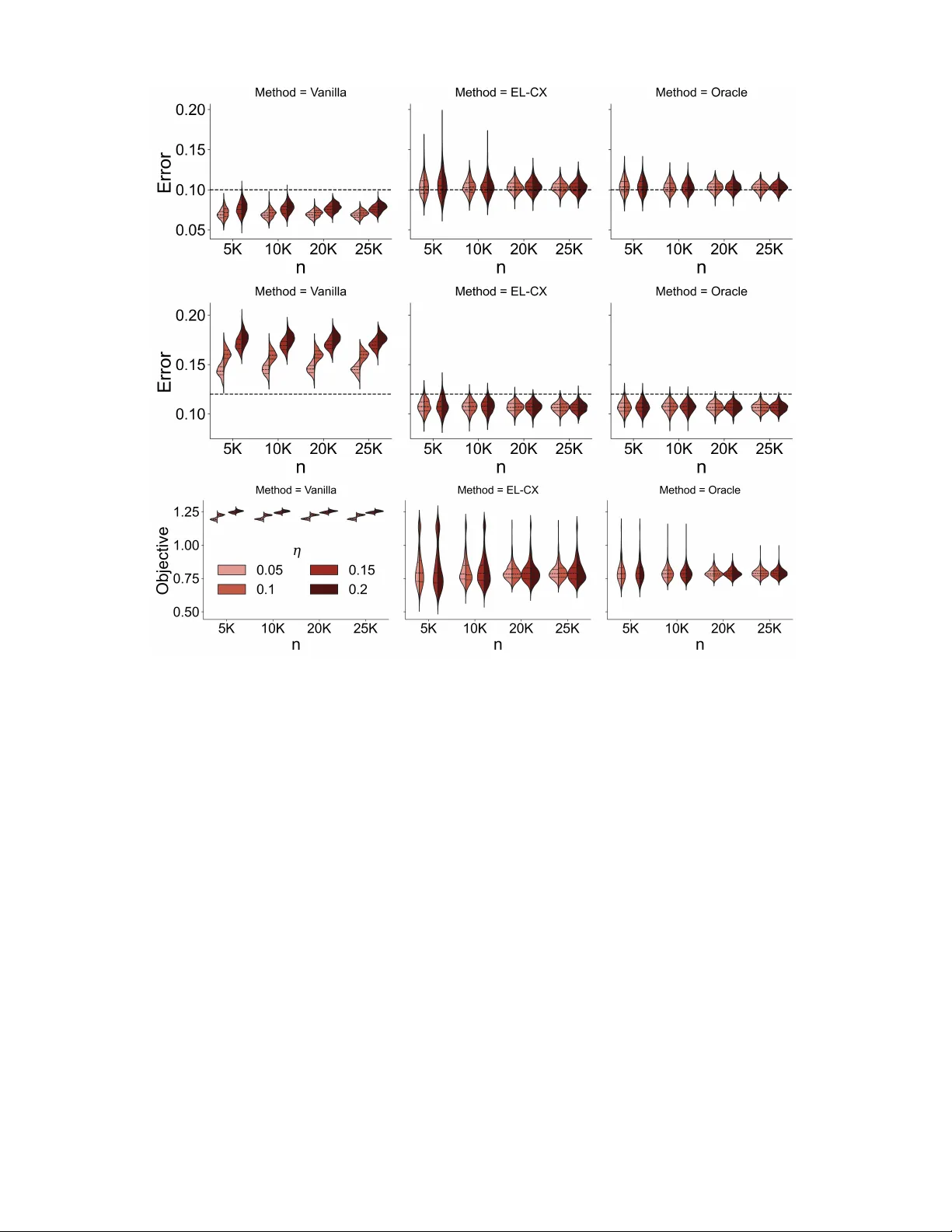
Neyman-P earson multiclass classiﬁcation under label noise via empirical likelihood Qiong Zhang Institute of Statistics and Big Data, Renmin Uni versity of China Qinglong T ian and Pengfei Li * Department of Statistics and Actuarial Science, Uni versity of W aterloo March 24, 2026 Abstract In many classiﬁcation problems, the costs of misclassifying observ ations from dif ferent classes can be highly unequal. The Neyman–Pearson multiclass classiﬁcation (NPMC) frame work addresses this issue by minimizing a weighted misclassiﬁcation risk while imposing upper bounds on class-speciﬁc error probabilities. Existing NPMC methods typically assume that training labels are correctly observed. In practice, ho wev er , labels are often corrupted due to measurement error or annotation, and the ef fect of such label noise on NPMC procedures remains largely unexplored. W e study the NPMC problem when only noisy labels are av ailable in the training data. W e propose an empirical likelihood (EL)–based method that relates the distributions of noisy and true labels through an exponential tilting density ratio model. The resulting maximum EL estimators recover the class proportions and posterior probabilities of the clean labels required for error control. W e establish consistenc y , asymptotic normality , and optimal con ver gence rates for these estimators. Under mild conditions, the resulting classiﬁer satisﬁes NP oracle inequalities with respect to the true labels asymptotically . An expectation–maximization algorithm computes the maximum EL estimators. Simulations sho w that the proposed method performs comparably to the oracle classiﬁer under clean labels and substantially improv es over procedures that ignore label noise. K e ywor ds: Corrupted labels, Data contamination, Density ratio model, Empirical likelihood, Supervised learning * Correspondence to: Pengfei Li pengfei.li@uwaterloo.ca . 1 1 Intr oduction In many real-world machine learning applications, especially in high-stakes domains such as medical diagnosis and ﬁnancial fraud detection, the consequences of dif ferent classiﬁcation errors are highly asymmetric. For instance, misclassifying a malignant tumor as benign can be far more consequential than the opposite error ( Bokhari et al. 2021 ), and approving a fraudulent loan carries greater risk than rejecting a legitimate one. T raditional classiﬁers, which typically minimize the ov erall misclassiﬁcation rate and treat all errors equally , do not account for such asymmetries. The Neyman–Pearson multiclass classiﬁcation (NPMC) frame work addresses this limitation by explicitly constraining error rates for selected classes, thereby prioritizing safety and reliability ov er simple accuracy . Speciﬁcally , let ( X , Y ) be a pair of random v ariables where X ∈ X ⊂ R p denotes the feature vector and Y ∈ [ K ] = { 0 , 1 , . . . , K − 1 } is the class label. F or each k , let P ∗ k ( A ) := P ( X ∈ A | Y = k ) for any Borel set A ⊂ X , and denote X k ≜ X | ( Y = k ) ∼ P ∗ k . The NPMC problem 1 seeks a classiﬁer ϕ : X → [ K ] that solv es: min ϕ L ( ϕ ) = K − 1 X k =0 ρ k P ∗ k ( { ϕ ( X )  = k } ) subject to P ∗ k ( { ϕ ( X )  = k } ) ≤ α k , ∀ k ∈ S ⊂ [ K ] , (1) where ρ k , α k , and S are pre-speciﬁed weights, target error lev els, and class indices with constrained errors, respecti vely . When K = 2 , problem ( 1 ) reduces to the classical Neyman–Pearson binary classiﬁcation task: minimizing the type II error while controlling the type I error . This binary setting has been extensi vely studied; see, for e xample, Scott & No wak ( 2005 ), Scott ( 2007 ), Rigollet & T ong ( 2011 ), T ong ( 2013 ), Zhao et al. ( 2016 ), T ong et al. ( 2018 , 2020 ), Li et al. ( 2020 ), Xia et al. ( 2021 ), W ang et al. ( 2024 ). In contrast, the general multiclass case ( K ≥ 3 ) remains relati vely underexplored. Extending binary NP classiﬁcation to the multiclass setting is non-tri vial, in part because problem ( 1 ) may be infeasible for certain speciﬁcations of ρ k and α k . Recently , T ian & Feng ( 2025 ) proposed a dual-based algorithm that checks asymptotic feasibility and pro vides an ef ﬁcient solver when strong duality holds. Their estimator further satisﬁes an NP oracle inequality , 1 The NPMC problem reduces to classical o verall misclassiﬁcation error minimization when ρ k = w ∗ k = P ( Y = k ) for all k and S = ∅ . 2 which compares the learned classiﬁer b ϕ to the oracle classiﬁer ϕ ∗ that satisﬁes the error constraints: P ∗ k ( { b ϕ ( X )  = k } ) ≤ P ∗ k ( { ϕ ∗ ( X )  = k } ) + O p ( ε ( n )) , ∀ k ∈ S (2) where ε ( n ) v anishes as the sample size n increases. Despite its appeal, the NPMC frame work fundamentally relies on clean, correctly labeled training data. This assumption is often violated in practice due to measurement error, annotator incon- sistency , or adv ersarial noise. Empirical studies suggest that roughly 5% of labels in real-world datasets are incorrect ( Y ao et al. 2023 ). Label noise is present e ven in standard benchmarks: for instance, Northcutt et al. ( 2021 ) ﬁnd mislabeling in datasets ranging from MNIST to ImageNet. In domain-speciﬁc datasets such as CheXpert ( Irvin et al. 2019 ), ambiguities in radiology reports can also result in erroneous labels. More recently , in applications in volving lar ge language models, stochastic v ariability in model outputs has been shown to induce label noise relativ e to an underly- ing latent ground truth, further illustrating the pervasi veness of noisy labels in modern machine learning systems ( Zhang & Martinez 2025 ). It is therefore natural to ask: What are the consequences of label noise for the NPMC problem? In the binary case, Y ao et al. ( 2023 ) showed that ignoring label noise can lead to overly conservative type I err or and thus an inﬂated type II err or . Their approach, ho wev er , requires prior kno wledge of the noise transition (confusion) matrix—the conditional probability of a noisy label given the true label—which is rarely a vailable in practice. Moreo ver , extending such results to the multiclass setting is also non-trivial. More broadly , it remains unclear how label noise impacts the general NPMC framework and how it can be properly accounted for , a gap that this paper aims to ﬁll. Concretely , suppose we observe n independently and identically distributed (i.i.d.) samples { ( X i , Y i , e Y i ) } n i =1 ∼ P ∗ X,Y , e Y , where Y i denotes the unknown true label and e Y i is a noisy version of Y i . In practice, we only observe the noisy training set D train = { ( X i , e Y i ) } n i =1 , along with m additional i.i.d. feature-only samples D test = X i i = n + 1 n + m from the same distribution. Our goal is to use only the noisy D train to learn a classiﬁer b ϕ such that its predictions on D test satisfy the constraints in ( 1 ) with respect to the (unobserved) true labels { Y i } n + m i = n +1 . W e propose a no vel empirical lik elihood (EL) framew ork for solving the NPMC problem under label noise, without requiring prior kno wledge of the noise transition matrix. Our method captures 3 the relationship between the true and noisy label distributions through an exponential tilting density ratio model (DRM). By estimating the DRM parameters, we recov er the key quantities–true class proportions and posterior probabilities of the clean labels–needed for error control under clean labels, which allo ws us to directly apply the clean-label error control procedure of T ian & Feng ( 2025 ) to the noisy-label setting. Computationally , we treat the true labels as latent v ariables and de velop an ef ﬁcient expectation–maximization algorithm to maximize the proﬁle empirical likelihood and consistently estimate these quantities. The proposed method has se veral k ey adv antages. First, it eliminates the need for an y prior kno wledge or bounds on the noise parameters, enhancing practical feasibility . Second, the resulting maximum empirical likelihood estimators are statistically consistent and asymptotically normal with optimal con v ergence rates. Third, under mild assumptions, we pro vide rigorous theoretical guarantees showing that the ﬁnal classiﬁer satisﬁes NP oracle inequalities. Fourth, simulation studies demonstrate that our method achiev es near-oracle performance—closely matching the error control of classiﬁers trained on clean labels—while signiﬁcantly outperforming naiv e approaches that ignore label noise. Finally , our frame work naturally accommodates both binary and multiclass classiﬁcation, thereby ﬁlling a notable gap in the existing literature. The rest of the paper is organized as follo ws. Section 2 introduces the problem setup and the relationship between noisy and clean labels. Section 3 presents the proposed EL-based estimator , its asymptotic normality , and the EM algorithm. Section 4 studies the binary NP problem, including the classiﬁer , oracle guarantees, and empirical results. Section 5 extends the framew ork to the general NPMC setting. Section 6 presents real-data results, and Section 7 concludes. 2 Pr oblem setting T o enable v alid statistical inference, we must formalize the relationship between latent Y and observed e Y . Follo wing established work ( Angluin & Laird 1988 , Y ao et al. 2023 , Sesia et al. 2024 , Bortolotti et al. 2025 ), we adopt the standard instance independence assumption: Assumption 2.1 (Instance-independent noise) . e Y ⊥ ⊥ X | Y (i.e., the noisy label e Y is conditionally independent of featur es X given the true label Y ). This assumption captures the common scenario as sho wn in Sesia et al. ( 2024 , Appendix A.3) 4 where label noise depends primarily on class membership rather than speciﬁc feature values, as frequently observ ed in real-world settings like crowdsourcing ( Snow et al. 2008 ). Beyond its practical relev ance, this assumption provides crucial tractability by establishing a clear relationship between the contaminated distrib ution e P ∗ k of f X k and the true conditional distrib ution P ∗ k of X k , as formalized in the proposition belo w . Proposition 2.1 (Distrib utional relationships under label noise) . Let e w ∗ l = P ( e Y = l ) and w ∗ k = P ( Y = k ) denote the noisy and true class pr oportions, r espectively . Let π ∗ k ( x ) = P ( Y = k | X = x ) and e π ∗ l ( x ) = P ( e Y = l | X = x ) . Deﬁne: • M ∗ : The confusion matrix with entries M ∗ lk = P ( Y = k | e Y = l ) , • T ∗ : The noise transition matrix with entries T ∗ lk = P ( e Y = l | Y = k ) = e w ∗ l M ∗ lk /w ∗ k . Then, under Assumption 2.1 , the following r elationships hold: (Mar ginal) w ∗ k = X l ∈ [ K ] M ∗ lk e w ∗ l , e w ∗ l = X k ∈ [ K ] T ∗ lk w ∗ k , (3) (Conditional) e P ∗ l = X k ∈ [ K ] M ∗ lk P ∗ k , P ∗ k = X l ∈ [ K ] T ∗ lk e P ∗ l , (4) (P osterior) e π ∗ l ( x ) = X k ∈ [ K ] T ∗ lk π ∗ k ( x ) . (5) The proof is deferred to Appendix C.1 . Remark 2.1. The pr oposition demonstr ates a fundamental duality: the pair ( M ∗ , f w ∗ ) contains equivalent information to ( T ∗ , w ∗ ) . This means we can focus our estimation efforts on either parameter gr oup, as the other can be derived accor dingly . W e consider ( T ∗ , w ∗ ) since w ∗ is used dir ectly in the NPMC numerical solver as we show in Section 5.1 . Based on these relationships, a nai ve two-step approach to estimating π ∗ k ( x ) via ( 5 ) would require prior kno wledge of the transition matrix T ∗ , which is typically una v ailable in practice. Instead, we propose a joint estimation procedure that simultaneously learns T ∗ and π ∗ k ( x ) by directly le veraging these distrib utional relationships, which we detail in the next section. 5 3 Empirical likelihood based estimation under label noise Since we observe contaminated labels e Y ∈ [ K ] rather than the true labels Y in the noisy label setting. Con ventional approaches that ignore this label noise yield estimators for { e w ∗ k , e π ∗ k ( x ) } K − 1 k =0 , which dif fer from the tar get quantities { w ∗ k , π ∗ k ( x ) } K − 1 k =0 needed for proper NP type error control. T o address this, we propose a ﬂe xible approach that directly estimates { w ∗ k , π ∗ k ( x ) } K − 1 k =0 from noisy labeled data. Our approach uses density ratio modeling and empirical likelihood, without r equiring any prior knowledge of the label corruption probabilities. This section presents our estimator along with its numerical computation and statistical properties for general classiﬁcation problems with label noise. 3.1 Exponential tilting and density ratio model Consider ( X , Y , e Y ) where ( X , Y ) ∼ P ∗ X,Y and e Y satisﬁes Assumption 2.1 . Let g ( x ) ∈ R d be some representation of feature x such that: π ∗ k ( x ) := P ( Y = k | X = x ) = exp(( γ ∗ k ) † + ⟨ β ∗ k , g ( x ) ⟩ ) P k ′ ∈ [ K ] exp(( γ ∗ k ′ ) † + ⟨ β ∗ k ′ , g ( x ) ⟩ ) . (6) with ( γ ∗ 0 ) † = 0 and β ∗ 0 = 0 for identiﬁability . This leads to the exponential tilting relationship between the class-conditional distributions: dP ∗ k dP ∗ 0 ( x ) = exp( γ ∗ k + ⟨ β ∗ k , g ( x ) ⟩ ) , (7) where dP ∗ k /dP ∗ 0 denotes the Radon-Nikodym deri v ati ve of P ∗ k with respect to P ∗ 0 , γ ∗ k = ( γ ∗ k ) † + log( w ∗ 0 /w ∗ k ) . W ith this reparameterization, we also ha ve γ ∗ 0 = 0 . T o ensure P ∗ k s are v alid probability measures, the parameters γ ∗ = { γ ∗ k } K − 1 k =1 and β ∗ = { β ∗ k } K − 1 k =1 must satisfy the constraints: Z exp( γ ∗ k + ⟨ β ∗ k , g ( x ) ⟩ ) P ∗ 0 ( dx ) = 1 , ∀ k ∈ 1 , . . . , K − 1 . (8) Under the instance-independent noise assumption (Assumption 2.1 ), the contaminated distrib utions of f X l ≜ X | ( e Y = l ) ∼ e P ∗ l relate to the true distributions as follo ws: d e P ∗ l dP ∗ 0 ( x ) = X k ∈ [ K ] M ∗ lk dP ∗ k dP ∗ 0 ( x ) = 1 e w ∗ l X k ∈ [ K ] { w ∗ k T ∗ lk exp( γ ∗ k + ⟨ β ∗ k , g ( x ) ⟩ ) } . (9) 6 Both ( 7 ) and ( 9 ) are instances of the density ratio model (DRM) ( Anderson 1979 , Qin 2017 ), where all measures ( { e P ∗ l } K − 1 l =0 , { P ∗ k } K − 1 k =1 ) are connected to the base measure P ∗ 0 via a parametric form. The DRM is highly ﬂe xible and encompasses many commonly used distribution families, including all members of the exponential f amily with appropriate speciﬁcations for P ∗ 0 and g ( x ) . For example, if the base distrib ution is normal and g ( x ) = ( x, x 2 ) ⊤ , the DRM reduces to the normal distribution f amily . Remark 3.1 (Basis function selection) . The function g is commonly referr ed to as the basis function. In our simulations and e xperiments, the simple c hoice g ( x ) = x performs well acr oss a range of scenarios. F or mor e complex data, suc h as imag es, performance may be impr oved by using featur es e xtracted fr om pr etrained deep neur al networks or by adopting data-adaptive appr oac hes, such as that of Zhang & Chen ( 2022 ). 3.2 Identiﬁability In this section, we study the identiﬁability of the model in ( 9 ) . W e emphasize that, in the absence of additional structural assumptions, the model is fundamentally unidentiﬁable—beyond the usual label permutation ambiguity encountered in mixture models. In particular , multiple distinct parameterizations can induce exactly the same observ ed distrib utions. W e illustrate this issue through two e xamples below . Example 3.1 (Algebraic unidentiﬁability of true distributions) . Consider a binary classiﬁcation pr oblem ( K = 2 ) wher e we observe noisy distributions e P 0 ( x ) and e P 1 ( x ) . Let the true underlying distributions be P ∗ 0 ( x ) and P ∗ 1 ( x ) , and let the true noise transition matrix be M ∗ , such that: e P 0 ( x ) = (1 − ρ ∗ 0 ) P ∗ 0 ( x ) + ρ ∗ 1 P ∗ 1 ( x ) , e P 1 ( x ) = ρ ∗ 0 P ∗ 0 ( x ) + (1 − ρ ∗ 1 ) P ∗ 1 ( x ) , wher e ρ ∗ 0 = P ( e Y = 1 | Y = 0) and ρ ∗ 1 = P ( e Y = 0 | Y = 1) . If P ∗ 0 ( x ) and P ∗ 1 ( x ) ar e unconstrained, the model is unidentiﬁable. F or any small constant ϵ ∈ (0 , 1) , we can deﬁne a new , "contaminated" candidate distribution for class 1: P ∗∗ 1 ( x ) ≜ (1 − ϵ ) P ∗ 1 ( x ) + ϵP ∗ 0 ( x ) . Because P ∗∗ 1 ( x ) is a con vex combination of two valid pr obability density functions, it is also a 7 valid density function. W e can re write the true P ∗ 1 ( x ) in terms of this new distrib ution: P ∗ 1 ( x ) = 1 1 − ϵ P ∗∗ 1 ( x ) − ϵ 1 − ϵ P ∗ 0 ( x ) . Substituting this back into the equation for the observed e P 0 ( x ) , we obtain: e P 0 ( x ) = (1 − ρ ∗ 0 ) P ∗ 0 ( x ) + ρ ∗ 1  1 1 − ϵ P ∗∗ 1 ( x ) − ϵ 1 − ϵ P ∗ 0 ( x )  , =  1 − ρ ∗ 0 − ϵρ ∗ 1 1 − ϵ  P ∗ 0 ( x ) +  ρ ∗ 1 1 − ϵ  P ∗∗ 1 ( x ) . Let ρ ∗∗ 1 = ρ ∗ 1 1 − ϵ and (1 − ρ ∗∗ 0 ) = 1 − ρ ∗ 0 − ϵρ ∗ 1 1 − ϵ . As long as ϵ is chosen to be suf ﬁciently small such that ρ ∗∗ 1 < 1 and (1 − ρ ∗∗ 0 ) > 0 , the new par ameters { ρ ∗∗ 0 , ρ ∗∗ 1 , P ∗ 0 ( x ) , P ∗∗ 1 ( x ) } ar e perfectly valid and satisfy the mixtur e equations to pr oduce the exact same observed distributions e P 0 ( x ) and e P 1 ( x ) . Ther efor e , the true noise rates and class-conditional distributions are non-identiﬁable without further structural assumptions. Example 3.2 (Unidentiﬁability due to linearly dependent features) . Recall our density ratio model formulation fr om ( 7 ) : dP ∗ 1 dP ∗ 0 ( x ) = exp( γ ∗ 1 + ⟨ β ∗ 1 , g ( x ) ⟩ ) . Suppose the c hosen featur e r epr esentation g ( x ) = ( g 1 ( x ) , g 2 ( x )) ⊤ ∈ R 2 is not linearly indepen- dent acr oss the support of P ∗ 0 . Speciﬁcally , assume the data strictly lies on a manifold wher e g 1 ( x ) + g 2 ( x ) = c for some constant c . Let ( γ ∗ 1 , β ∗ 11 , β ∗ 12 ) be the true parameter s generating the data. The exponential tilt is: γ ∗ 1 + β ∗ 11 g 1 ( x ) + β ∗ 12 g 2 ( x ) . Now , consider a dif fer ent set of parameter s deﬁned by shifting the featur e coefﬁcients by an arbitrary constant δ  = 0 : β ∗∗ 11 = β ∗ 11 + δ, β ∗∗ 12 = β ∗ 12 + δ. Evaluating the tilt with these new par ameters yields: γ ∗ 1 + β ∗∗ 11 g 1 ( x ) + β ∗∗ 12 g 2 ( x ) = γ ∗ 1 + ( β ∗ 11 + δ ) g 1 ( x ) + ( β ∗ 12 + δ ) g 2 ( x ) = γ ∗ 1 + β ∗ 11 g 1 ( x ) + β ∗ 12 g 2 ( x ) + δ ( g 1 ( x ) + g 2 ( x )) = ( γ ∗ 1 + δ c ) + β ∗ 11 g 1 ( x ) + β ∗ 12 g 2 ( x ) . 8 By deﬁning a new baseline par ameter γ ∗∗ 1 = γ ∗ 1 + δ c , we perfectly absorb the shift. The pa- rameter sets ( γ ∗ 1 , β ∗ 11 , β ∗ 12 ) and ( γ ∗∗ 1 , β ∗∗ 11 , β ∗∗ 12 ) pr oduce the exact same density r atio exp( γ ∗∗ 1 + ⟨ β ∗∗ 1 , g ( x ) ⟩ ) ≡ exp( γ ∗ 1 + ⟨ β ∗ 1 , g ( x ) ⟩ ) for all observable x . Thus, without assumptions guaranteeing the richness of t he featur e subspace (i.e., ruling out collinearity), the e xponential tilt par ameters ar e non-identiﬁable. These examples highlight that the model is intrinsically unidentiﬁable without further structural constraints. T o resolv e this issue, we impose a set of mild but essential assumptions that ensure identiﬁability , as stated in the following theorem. Theorem 3.1 (Identiﬁability) . Under mild assumptions (Assumptions C.1 – C.3 ), the parameters ( M ∗ , γ ∗ , β ∗ ) and the r efer ence distrib ution P ∗ 0 in ( 9 ) ar e strictly identiﬁable. Strict identiﬁability implies a true one-to-one mapping between the parameter space and the probability distributions of the observed data. For our model, this means there is exactly one unique set of parameters ( M ∗ , γ ∗ , β ∗ ) and one unique reference distribution P ∗ 0 that can generate the observed data, completely eliminating the label-switching (permutation) ambiguity that typically plagues mixture models. T o establish this strict identiﬁability , we require three standard regularity conditions. Broadly , these conditions ensure that the latent mixture components are physically distinct and that the observed data provides suf ﬁcient variation to decouple them. Speciﬁcally , we require the feature coefﬁcients of the e xponential tilts to be strictly distinct (Assumption C.1 ) and the feature mapping to explore a suf ﬁciently rich subspace (Assumption C.2 ). These are common requirements in the exponential f amily and ﬁnite mixture model literature to pre vent component collapse and guarantee that the underlying densities are linearly independent. Furthermore, we require the confusion matrix M ∗ to be full rank, with speciﬁc structural constraints on its in verse (Assumption C.3 ). Crucially , this ﬁnal condition on the in verse matrix not only ensures the signal from the true latent components is preserv ed, but it ef fecti vely breaks the permutation sym metry inherent in standard mixture models, allo wing for the strict, unique identiﬁcation of all parameters. The formal mathematical statements of these assumptions, along with the complete proof, are deferred to Appendix C.4 . 9 3.3 Empirical likelihood based infer ence T o a void restricti ve parametric assumptions on the base distribution, we adopt a non-parametric approach on the estimation of π ∗ k ( x ) and the rest of the parameters T ∗ and w ∗ , gi ven a set of i.i.d. samples { ( X i , e Y i ) } n i =1 from P ∗ X, e Y . The log-likelihood function based on the contaminated set D = { ( X i , e Y i ) } n i =1 i.i.d. ∼ P ∗ X, e Y is ℓ = n X i =1 K − 1 X l =0 h 1 ( e Y i = l ) log n e w ∗ l e P ∗ l ( { X i } ) oi . Using the exponential tilting relationship in ( 9 ), we obtain ℓ = n X i =1 X l ∈ [ K ] 1 ( e Y i = l ) log   X k ∈ [ K ] { w ∗ k T ∗ lk exp( γ ∗ k + ⟨ β ∗ k , g ( X i ) ⟩ ) }   + n X i =1 log P ∗ 0 ( { X i } ) . The empirical likelihood (EL) ( Owen 2001 , Qin & La wless 1994 ) allows us to estimate parameters without assumptions on the form of P ∗ 0 . Speciﬁcally , let p i = P ∗ 0 ( { X i } ) for i = 1 , . . . , n and vie w them as parameters. Let w = { w k } K − 1 k =0 and θ = { w , γ , β , T } . The log-EL function becomes: ℓ ( p , θ ) = n X i =1 X l ∈ [ K ] 1 ( e Y i = l ) log   X k ∈ [ K ] n w k T lk exp( γ k + β ⊤ k g ( X i )) o   + n X i =1 log p i . (10) The feasible v alues of p must satisfy the following constraints: p i ≥ 0 , n X i =1 p i = 1 , n X i =1 p i exp( γ k + β ⊤ k g ( X i )) = 1 , ∀ k = 1 , . . . , K − 1 . (11) The ﬁrst two conditions in ( 11 ) ensure that P ∗ 0 is a valid probability measure, while the last follo ws from ( 8 ). The inference for θ is usually made by ﬁrst proﬁling the log-EL with respect to p . That is, we deﬁne pℓ n ( θ ) = sup p ℓ n ( p , θ ) subject to the constraints in ( 11 ) . By the Lagrange multiplier method (see Appendix C.2 for details), the maximizer is attained when p i = p i ( θ ) = n − 1 " 1 + K − 1 X k =1 ν k n exp( γ k + β ⊤ k g ( X i )) − 1 o # − 1 (12) where the Lagrange multipliers ν 1 , . . . , ν K − 1 are the solution to n X i =1 exp( γ k + β ⊤ k g ( X i )) − 1 1 + P K − 1 k ′ =1 ν k ′ n exp( γ k ′ + β ⊤ k ′ g ( X i )) − 1 o = 0 , k = 1 , . . . , K − 1 . (13) 10 The proﬁle log-EL of θ (after maximizing out p i ) is gi ven by pℓ n ( θ ) = n X i =1 X l ∈ [ K ] 1 ( e Y i = l ) log   X k ∈ [ K ] n w k T lk exp( γ k + β ⊤ k g ( X i )) o   + n X i =1 log p i ( θ ) , and the Maximum Empirical Likelihood Estimator (MELE) of θ is deﬁned as b θ = arg max pℓ n ( θ ) . (14) The conditional distribution estimators are then b P k = n X i =1 p i ( b θ ) exp( b γ k + b β ⊤ k g ( X i )) δ X i , b π k ( x ) = exp( b γ † k + b β ⊤ l g ( x )) P k ′ exp( b γ † k ′ + b β ⊤ k ′ g ( x )) , (15) where b γ † k = b γ k + log ( b w 0 / b w k ) . 3.4 Statistical guarantees Theorem 3.2 (Estimator rate of con vergence) . Let θ ∗ = ( w ∗ , γ ∗ , β ∗ , T ∗ ) be the true values of θ and b θ be its MELE estimator in ( 14 ) . W e have √ n ( b θ − θ ∗ ) → N (0 , Σ) as n → ∞ wher e Σ > 0 is some non-de g enerated covariance matrix. The proof of the theorem is deferred to Appendix C.3 . The result establishes that the MELE estimator is consistent and asymptotically normal, achie ving the optimal con ver gence rate. This asymptotic normality plays a key role in deri ving the NP oracle inequalities for the ﬁnal classiﬁer . 3.5 EM algorithm f or proﬁle EL maximization Since the true labels ( Y 1 , . . . , Y n ) are unobserved, e P ∗ l become mixtures of P ∗ 0 , . . . , P ∗ K − 1 . This complicates the maximization of ( 14 ) due to non-con ve xity . T o address the challenge, we treat the true labels as missing v alues and employ an Expectation-Maximization (EM) algorithm for its numerical computation. W e summarize the algorithm in Algorithm 1 and explain it belo w . The EM frame work is particularly well-suited for problems with latent variables, as it iterati v ely handles the missing information via: an expectation step that computes conditional probabilities of the missing true labels; a maximization step that updates parameter estimates. 11 Algorithm 1 EM algorithm for classiﬁcation with noisy labels via empirical likelihood Input: Noisy labeled data { ( X i , e Y i ) } n i =1 , feature mapping g ( x ) , number of classes K , con v ergence threshold ϵ Output: Estimates b w k , b π k ( x ) for all k ∈ [ K ] 1: Initialize: Choose initial parameters θ (0) = ( w (0) , γ (0) , β (0) , T (0) ) Set initial proﬁle log-EL pℓ n ( θ (0) ) ← −∞ 2: repeat 3: E-step: Compute posterior probabilities ω ( t ) ik for each observ ation according to ( 16 ) 4: M-step: Update parameters: 5: Update class proportions w ( t +1) k via ( 17 ) 6: Update transition matrix T ( t +1) via ( 18 ) 7: Update ( ¯ γ ( t +1) , β ( t +1) ) by solving the weighted multinomial logistic regression in ( 19 ) 8: Adjust and update to obtain γ ( t +1) k ← ¯ γ ( t +1) k − log ( P n i =1 ω ( t ) ik / P n i =1 ω ( t ) i 0 ) 9: Update weights p ( t +1) i via ( 21 ) to compute pℓ n ( θ ( t +1) ) 10: until pℓ n ( θ ( t +1) ) − pℓ n ( θ ( t ) ) < ϵ 11: Return: b w k ← w ( t +1) k , b π k ( x ) ← exp( b γ † k + b β ⊤ k g ( x )) P k ′ exp( b γ † k ′ + b β ⊤ k ′ g ( x )) where b γ † k = γ ( t +1) k + log w ( t +1) 0 w ( t +1) k If the complete data { ( X i , Y i , e Y i ) } n i =1 were av ailable, the complete data log-EL would be ℓ c n ( p , θ ) = n X i =1 X l ∈ [ K ] X k ∈ [ K ] 1 ( e Y i = l , Y i = k ) log P ( X = X i , e Y i = l , Y i = k ) . Using the chain rule and the instance-independent Assumption 2.1 , we decompose the joint probability into: P ( X = X i , e Y i = l , Y i = k ) = P ( X = X i | e Y i = l , Y i = k ) P ( e Y i = l | Y i = k ) P ( Y i = k ) = P ( X = X i | Y i = k ) T ∗ lk w ∗ k = P ∗ 0 ( { X i } ) exp { γ ∗ k + ⟨ β ∗ k , g ( X i ) ⟩} T ∗ lk w ∗ k , where the last equality is from the DRM in ( 7 ). This yields the complete data proﬁle log-EL: ℓ c n ( p , θ ) = n X i =1 X l ∈ [ K ] X k ∈ [ K ] 1 ( e Y i = l ) 1 ( Y i = k ) h log p i + { γ k + β ⊤ k g ( X i ) } + log T lk + log w k i . W e deﬁne the proﬁle complete data log-EL as pℓ c n ( θ ) = sup p ℓ c n ( p , θ ) 12 where the maximization is subject to the constraints in ( 11 ) . Using the same deri v ation for ( 12 ) , the proﬁle complete data log-EL becomes pℓ c n ( θ ) = n X i =1 X l ∈ [ K ] X k ∈ [ K ] 1 ( e Y i = l ) 1 ( Y i = k )  γ k + β ⊤ k g ( X i ) + log T lk + log w k  + n X i =1 log p i ( θ ) where p i ( θ ) is gi ven in ( 12 ), and the ν k ’ s are the solutions to ( 13 ). The EM algorithm is an iterati ve procedure that starts with an initial guess θ (0) . At each iteration t , gi ven the current parameter estimate θ ( t ) , the algorithm proceeds in two steps: • E-step (Expectation step) : The missing data is “ﬁlled in” by computing an educated guess based on the current parameter estimate θ ( t ) . This in volv es calculating the posterior distribution of the missing data gi ven the observed data and the current parameters: ω ( t ) ik = E ( 1 ( Y i = k ) | θ ( t ) ; e Y i , X i ) = P ( Y i = k | θ ( t ) ; e Y i , X i ) = exp( γ ( t ) k + ⟨ β ( t ) k , g ( X i ) ⟩ ) T ( t ) e Y i ,k w ( t ) k P K k ′ =1 exp( γ ( t ) k ′ + ⟨ β ( t ) k ′ , g ( X i ) ⟩ ) T ( t ) e Y i ,k ′ w ( t ) k ′ . (16) Then the expected complete data proﬁle empirical log-EL at iteration t is Q ( θ ; θ ( t ) ) = E { pℓ ( c ) n ( θ ) | θ ( t ) ; D } = n X i =1 X l ∈ [ K ] 1 ( e Y i = l ) X k ∈ [ K ] ω ( t ) ik (log w k + γ k + β ⊤ k g ( X i ) + log T lk ) + n X i =1 log p i ( θ ) • M-step (Maximization step) : Instead of maximizing log-EL, the M-step maximizes Q with respect to θ instead, i.e., θ ( t +1) = arg max Q ( θ , θ ( t ) ) . Since Q is separable in w , T , and ( γ , β ) , we can optimize each set of parameters separately . Belo w are the updated parameters; the detailed deriv ations are provided in Appendix A.1 . w ( t +1) k = 1 n n X i =1 ω ( t ) ik (17) T ( t +1) lk = P n i =1 1 ( e Y i = l ) ω ( t ) ik P n i =1 ω ( t ) ik . (18) The update of ( γ ( t +1) , β ( t +1) ) is slightly more complicated. Note that ( γ ( t +1) , β ( t +1) ) maximizes the function Q 3 ( γ , β ; θ ( t ) ) = n X i =1 X k ∈ [ K ] ω ( t ) ik ( γ k + β ⊤ k g ( X i )) − n X i =1 log ( 1 + K − 1 X k =1 ν k  exp( γ k + β ⊤ k g ( X i )) − 1  ) . 13 At the optimal point, we sho w in Appendix A.1 that the Lagrange multipliers ν k = n − 1 n X i =1 ω ( t ) ik := ω ( t ) · k . Thus, the stationary point of Q 3 ( γ , β ; θ ( t ) ) coincides with the stationary point of e Q ( γ , β ; θ ( t ) ) = n X i =1 X k ∈ [ K ] ω ( t ) ik ( γ k + β ⊤ k g ( X i )) − n X i =1 log    X k ∈ [ K ] w · k exp( γ k + β ⊤ k g ( X i ))    . Let ¯ γ k = γ k + log ( ω ( t ) · k /ω ( t ) · 0 ) , then the function e Q becomes e Q ( ¯ γ , β ; θ ( t ) ) = n X i =1 X k ∈ [ K ] ω ( t ) ik ( ¯ γ k + β ⊤ k g ( X i )) − n X i =1 log    X k ∈ [ K ] exp( ¯ γ k + β ⊤ k g ( X i ))    , (19) which is the weighted log-likelihood of multinomial logistic re gression model based on the dataset in T able 4 in Appendix A.1 . Thus, ( ¯ γ ( t +1) , β ( t +1) ) maximizes the weighted log- likelihood. W e can use any e xisting packages in R or Python to ﬁnd the numerical value. Finally , we compute γ ( t +1) k = ¯ γ ( t +1) k − log ( ω ( t ) · k /ω ( t ) · 0 ) , k ∈ [ K ] . (20) The weights are p ( t +1) i = p i ( θ ( t +1) ) = n − 1    X k ∈ [ K ] ω ( t ) · k exp( γ ( t +1) k + ⟨ β ( t +1) k , g ( X i ) ⟩ )    − 1 (21) since ν k = ω ( t ) · k at the optimal point. The E-step and M-step are repeated iterativ ely until the change in the proﬁle log-EL falls below a predeﬁned threshold. This stopping criterion is guaranteed to be met because the EM algorithm produces a sequence of estimates that monotonically increases the true objecti ve—the proﬁle log-EL, which we detail belo w . Proposition 3.1 (Con v ergence of EM algorithm) . W ith the EM algorithm described above, we have for t ≥ 1 , pℓ n ( θ ( t +1) ) ≥ pℓ n ( θ ( t ) ) . The proof of Proposition 3.1 is giv en in Appendix A.2 . First note that pℓ n ( θ ( t +1) ) is a sum of the logarithm of probabilities, hence this implies that pℓ n ( θ ) ≤ 0 for any θ that is feasible. W ith this result, Proposition 3.1 guarantees that the EM algorithm ev entually con ver ges to at least a local maximum for the giv en initial v alue θ (0) . W e recommend using multiple initial values to 14 explore the likelihood function to ensure that the algorithm reaches the global maximum. Second, in practice, we may stop the algorithm when the increment in the log-EL after an iteration is no greater than, say , 10 − 6 . Remark 3.2 (Incorporating prior knowledge) . When prior knowledge about the transition matrix is available (e .g., T ∗ kk ≥ ξ k > 0 ), the EM algorithm’ s M-step can be modiﬁed to incorporate such prior information. The analytical solution for this constrained update is pr ovided in A.3 . T o further impr ove numerical stability and con ver gence speed, penalties can be imposed on the diagonal elements { T kk } K − 1 k =0 . The corr esponding analytical solution for this penalized update is detailed in Appendix A.4 . 4 Neyman-P earson binary classiﬁcation This section focuses on binary classiﬁcation, a fundamental setting widely used in practice. W e begin by revie wing the NP frame work for clean-label binary classiﬁcation, where the optimal classiﬁer is deriv ed from a likelihood ratio test. W e then incorporate the EL-based estimator from the pre vious section into this frame work to achiev e type I error control under noisy labels. The resulting classiﬁer prov ably controls the empirical type I error asymptotically . 4.1 Revisiting NP binary classiﬁcation with clean labels W e be gin by re vie wing the NP binary classiﬁcation frame work without label noise. Consider random variables ( X , Y ) ∼ P ∗ X,Y , where w ∗ = P ( Y = 1) , π ∗ ( x ) = P ( Y = 1 | X = x ) , and X y ≜ X | ( Y = y ) ∼ P ∗ y . For a classiﬁer ϕ : X → { 0 , 1 } , the NP paradigm solves: min ϕ P ∗ 1 ( { ϕ ( X )  = 1 } ) s.t. P ∗ 0 ( { ϕ ( X )  = 0 } ) ≤ α , (22) where α ∈ (0 , 1) is the desired type I error lev el, and the objecti ve represents the type II error . This formulation is a special case of the general NPMC problem in ( 1 ) with ρ 0 = 0 , ρ 1 = 1 , S = { 0 } , and α 0 = α . When the joint distribution P ∗ X,Y is known, the NP lemma ( Sadinle et al. 2019 , Lemma 1) 15 establishes that the optimal classiﬁer takes the form: ϕ ∗ λ ( x ) = 1 dP ∗ 1 dP ∗ 0 ( x ) ≥ λ ! = 1 ( λ ≤ r ( x, π ∗ , w ∗ )) (23) where r ( x, π , w ) = { (1 − w ) π ( x ) } / { w (1 − π ( x )) } . The v alue of λ controls the trade-off between type I and type II errors: a smaller λ increases the type I error while reducing the type II error . Using Bayes’ theorem and the law of total e xpectation, it can be sho wn that the optimal λ ∗ in ϕ ∗ λ is determined by solving: α = P ∗ 0 ( { ϕ ∗ λ ( X )  = 0 } ) = (1 − w ∗ ) − 1 E X [ { 1 − π ∗ ( X ) } 1 ( λ ≤ r ( X , π ∗ , w ∗ ))] . (24) At the sample leve l, let D = { ( X i , Y i ) } n i =1 i.i.d. ∼ P X,Y . Gi ven estimators b w and b π ( x ) for w and π ( x ) based on D , respecti vely , we estimate λ ∗ by solving the empirical estimate of ( 24 ): 1 n n X i =1 { 1 − b π ( X i ) } 1 ( λ ≤ r ( X i , b π , b w )) = α (1 − b w ) . (25) The left-hand side of ( 25 ) is piece wise constant in λ , with jumps at { r ( X i , b π , b w ) } n i =1 . The estimator b λ corresponds to the smallest jump point where the constraint is satisﬁed. Once b λ is obtained, we substitute it, along with the estimators for π ( x ) and w , into ( 23 ) to obtain the error-controlled classiﬁer , denoted as b ϕ b λ . 4.2 NP binary classiﬁcation with noisy labels with statistical guarantees Since our EL-based estimation allows us to directly estimate b w and b π from noisy labeled observa- tions, we can simply plug in these estimators, as discussed in the clean label case, to obtain the ﬁnal classiﬁer with controlled type I error . Speciﬁcally , let b w , b γ , b β be the MELE estimators deﬁned in ( 14 ) with b γ † = b γ + log { (1 − b w ) / b w } . W e deﬁne b π ( x ) = h 1 + exp( −{ b γ † + b β ⊤ g ( x ) } ) i − 1 . (26) Let b λ be the solution to ( 25 ) with the estimators b π and b w as deﬁned abo ve. Our ﬁnal binary classiﬁer with type I error control is gi ven by b ϕ b λ ( x ) = 1 ( b λ < r ( x, b π , b w )) = 1 b π ( x ) ≥ b λ b w 1 − b w + b λ b w ! , (27) 16 where the complete expression for the threshold is implied by the conte xt. W e no w show that the type I error of this estimator is asymptotically controlled at the target le vel. The follo wing assumptions are required for our theoretical results: Assumption 4.1 (Compactness) . The parameter space Θ = { ( γ , β ) : γ ∈ R , γ ∈ R d } is compact. Assumption 4.2 (Bounded second moment) . Ther e exists a constant R > 0 s.t. E ∥ g ( X ) ∥ 2 2 ≤ R 2 . Theorem 4.1 (Error control guarantee) . Let b ϕ b λ ( x ) be the binary classiﬁer deﬁned in ( 27 ) . Under Assumptions 4.1 and 4.2 , the type I err or is contr olled as follows: P ∗ 0 n b ϕ b λ ( X )  = 0 o ≤ α + O p ( n − 1 / 2 ) . The proof is deferred to Appendix C.6 . This theorem establishes that our classiﬁer asymptotically controls the type I error at the target le vel α under Assumptions 4.1 and 4.2 , which are standard in the literature (e.g., T ian & Feng 2025 ). These conditions are realistic in practice: Assumption 4.1 requires only that the parameter space be closed and bounded, which can be enforced by imposing | γ | + ∥ β ∥ 2 ≤ B for a sufﬁciently large B , while Assumption 4.2 demands only ﬁnite second moments of the feature map g ( X ) . Under these mild conditions, the Rademacher complexity of the class { π ( x ) : ( γ , β ) ∈ Θ } is of order n − 1 / 2 . Combined with the fact that our EL-based estimators ( b γ , b β , b w ) con ver ge at the usual n − 1 / 2 rate, this ensures that the ﬁnal classiﬁer b ϕ b λ preserves the Neyman–Pearson guarantee up to a v anishing O p ( n − 1 / 2 ) term. Remark 4.1 (NP umbrella algorithm type control) . The NP umbr ella algorithm was de veloped by T ong et al. ( 2018 ) to contr ol err ors in binary classiﬁcation with uncontaminated data, and later e xtended to the noisy-label setting by Y ao et al. ( 2023 ). When domain knowledg e of the noise transition matrix M ∗ is available, the y estimate the discr epancy between true and corrupted type I err or s and pr opose a label-noise-adjusted NP umbr ella algorithm with theor etical guarantees. Speciﬁcally , for any δ > 0 , they show that their classiﬁer ϕ δ satisﬁes P ( P ∗ 0 ( { ϕ δ ( X )  = 0 } ) ≤ α ) > 1 − δ + O ( ε ( n )) , (28) wher e ε ( n ) vanishes as n incr eases. T o our knowledge, this is the only work addr essing err or contr ol under noisy labels. It is ther efor e natur al to compar e our err or contr ol guar antee (Theo- r em 4.1 ) with their result. At ﬁrst glance, our guarantee appears weaker than that of Y ao et al. 17 ( 2023 ). In particular , we show that ∀ ϵ > 0 , ther e e xist constants C and N such that for all n ≥ N , P ( P ∗ 0 ( { b ϕ b λ ( X )  = 0 } ) ≤ α + C n − 1 / 2 ) > 1 − ϵ. Comparing this with ( 28 ) , the distinction lies in the quantities being contr olled. Our analysis bounds the deviation of the empirical type I err or fr om the tar get level, which intr oduces a stochastic ﬂuctuation of or der n − 1 / 2 . In contrast, the NP umbr ella fr amework pr ovides a stricter guarantee , ensuring with high pr obability that the population type I err or never e xceeds the tar get level. Importantly , our EL-based estimator is ﬂe xible and can be pair ed with differ ent err or contr ol methods: when combined with the NP umbr ella algorithm, it yields the same guarantee as in Y ao et al. ( 2023 ). Mor eover , our method does not requir e prior knowledge of M ∗ . Further discussion and empirical r esults ar e pr o vided in Appendix B.2.3 . 4.3 Simulation study In this section, we ev aluate the performance of our proposed classiﬁer ( 27 ) on simulated data and compare it with e xisting methods. Follo wing the e xperimental settings of Y ao et al. ( 2023 ), we consider three distinct distributions for the feature v ariables X y : • Case A: Gaussian distrib ution . Let X 0 ∼ N ( µ ∗ 0 , Σ ∗ ) and X 1 ∼ N ( µ ∗ 1 , Σ ∗ ) , where µ ∗ 0 = (0 , 0 , 0) ⊤ , µ ∗ 1 = (1 , 1 , 1) ⊤ , and Σ ∗ is a T oeplitz matrix with diagonal elements being 2 , ﬁrst of f-diagonal elements being − 1 , and remaining elements 0 . • Case B: Unif orm distribution within circles . Let X 0 and X 1 be uniformly distributed within unit circles centered at (0 , 0) ⊤ and (1 , 1) ⊤ , respecti vely . • Case C: t -distribution . Let X 0 and X 1 follo w multiv ariate non-central t -distributions with location parameters µ ∗ 0 and µ ∗ 1 , shape matrix Σ ∗ , and 15 degrees of freedom. The v alues of µ ∗ 0 , µ ∗ 1 , and Σ ∗ match those in Case A. Using the relationship e P ∗ 0 = m ∗ 0 P ∗ 0 + (1 − m ∗ 0 ) P ∗ 1 and e P ∗ 1 = m ∗ 1 P ∗ 0 + (1 − m ∗ 1 ) P ∗ 1 , where m ∗ 0 = P ( Y = 0 | e Y = 0) and m ∗ 1 = P ( Y = 0 | e Y = 1) represent the label corruption probabilities, we generate samples with corrupted labels. For each setting, we create a training sample of 2 n observ ations, equally split between the corrupted class 0 and corrupted class 1 . W e vary the sample size n from 1 , 000 to 5 , 000 to examine the ef fect of sample size on performance. T o accurately 18 approximate the true type I and type II errors, we generate a large e valuation set consisting of 20 , 000 true class 0 observ ations and 20 , 000 true class 1 observ ations. For each combination of distribution and sample size, we repeat the experiment R = 500 times and report the av erage type I and type II errors across all repetitions. T able 1: T ype I and II error for binary classiﬁcation based on 500 repetitions. NPC ∗ represents the oracle method with known m ∗ 0 and m ∗ 1 . For each setting, the method achieving type I error closest to the nominal le vel is highlighted in boldface. Case n m ∗ 0 = 0 . 95 , m ∗ 1 = 0 . 05 m ∗ 0 = 0 . 95 , m ∗ 1 = 0 . 05 m ∗ 0 = 0 . 9 , m ∗ 1 = 0 . 1 m ∗ 0 = 0 . 9 , m ∗ 1 = 0 . 1 α = 0 . 05 , δ = 0 . 05 α = 0 . 1 , δ = 0 . 1 α = 0 . 05 , δ = 0 . 05 α = 0 . 1 , δ = 0 . 1 V anilla NPC NPC ∗ Ours V anilla NPC NPC ∗ Ours V anilla NPC NPC ∗ Ours V anilla NPC NPC ∗ Ours T ype I error A 1000 0.011 0.010 0.027 0.051 0.049 0.045 0.076 0.101 0.004 0.003 0.024 0.052 0.025 0.022 0.073 0.102 2000 0.014 0.012 0.033 0.050 0.054 0.052 0.083 0.100 0.005 0.004 0.031 0.050 0.028 0.027 0.081 0.100 5000 0.017 0.016 0.039 0.050 0.058 0.056 0.089 0.100 0.006 0.005 0.038 0.050 0.031 0.030 0.088 0.100 B 1000 0.001 0.001 0.026 0.051 0.042 0.038 0.077 0.105 0.000 0.000 0.021 0.048 0.007 0.006 0.074 0.101 2000 0.002 0.002 0.033 0.051 0.047 0.046 0.083 0.104 0.000 0.000 0.029 0.047 0.010 0.009 0.081 0.101 5000 0.004 0.004 0.039 0.051 0.052 0.051 0.090 0.104 0.000 0.000 0.037 0.047 0.013 0.013 0.088 0.101 C 1000 0.014 0.012 0.028 0.062 0.051 0.048 0.077 0.112 0.007 0.006 0.026 0.063 0.029 0.027 0.075 0.114 2000 0.017 0.015 0.034 0.061 0.055 0.053 0.083 0.111 0.008 0.007 0.032 0.061 0.032 0.031 0.081 0.111 5000 0.019 0.018 0.039 0.060 0.059 0.058 0.089 0.111 0.009 0.009 0.038 0.061 0.035 0.034 0.088 0.111 T ype II error A 1000 0.534 0.567 0.398 0.278 0.287 0.305 0.218 0.171 0.689 0.730 0.427 0.277 0.403 0.427 0.227 0.171 2000 0.489 0.515 0.352 0.279 0.269 0.276 0.201 0.171 0.653 0.674 0.368 0.279 0.376 0.388 0.205 0.172 5000 0.459 0.470 0.319 0.278 0.254 0.260 0.188 0.171 0.622 0.630 0.326 0.279 0.357 0.363 0.190 0.171 B 1000 0.352 0.418 0.180 0.137 0.151 0.158 0.108 0.078 0.661 0.700 0.205 0.142 0.244 0.274 0.113 0.082 2000 0.268 0.310 0.164 0.137 0.143 0.145 0.100 0.079 0.610 0.637 0.172 0.143 0.212 0.221 0.103 0.082 5000 0.230 0.240 0.154 0.137 0.136 0.138 0.092 0.078 0.571 0.584 0.157 0.143 0.200 0.203 0.094 0.082 C 1000 0.588 0.629 0.461 0.282 0.321 0.341 0.247 0.176 0.722 0.755 0.487 0.280 0.440 0.462 0.255 0.176 2000 0.545 0.571 0.406 0.283 0.301 0.310 0.227 0.177 0.684 0.704 0.421 0.284 0.413 0.422 0.233 0.178 5000 0.514 0.525 0.369 0.283 0.286 0.291 0.213 0.176 0.656 0.666 0.378 0.282 0.392 0.399 0.214 0.176 For our method, we use linear basis functions in all experiments. These three cases are designed to e valuate both efﬁcienc y and robustness: the DRM assumption holds in Case A, whereas the model is misspeciﬁed in Cases B and C. W e compare our method with the V anilla and NPC algorithms proposed in Y ao et al. ( 2023 ). • V anilla : Ignores label noise and directly applies the NP paradigm to the noisy labeled data. • NPC/NPC ∗ : Both methods account for label noise. NPC ∗ knows the true m ∗ 0 and m ∗ 1 v alues, 19 while NPC assumes that the bounds m # 0 ≥ m ∗ 0 and m # 1 ≤ m ∗ 1 are kno wn. Follo wing the original method, NPC includes a parameter δ such that the type I error is controlled with probability at least 1 − δ . W e set m # 0 = max { m ∗ 0 + δ / 3 , 1 } and m # 1 = min { m ∗ 1 − δ / 3 , 0 } , and examine v arious combinations of ( m ∗ 0 , m ∗ 1 , δ, α ) . Throughout all experiments, we ﬁx g ( x ) = x for our algorithm. For the V anilla and NPC algorithms, we employ different base classiﬁers to estimate e π ( x ) ∗ : LD A for Case A and logistic re gression for Cases B and C. The complete experimental results are presented in T able 1 . The results demonstrate three ke y ﬁndings. First, the V anilla method prov es ov erly conservati v e in controlling type I error , resulting in substantially inﬂated type II error rates. Second, while both NPC and NPC ∗ successfully adjust for label noise, the y remain more conservati v e than our proposed approach. Notably , NPC ∗ –which le verages the kno wn values of m 0 and m 1 – outperforms NPC that relies on their bounds. In fact, when only bounds are av ailable, the NPC method can be as conservati ve as, or ev en more so than, the V anilla approach. Third, our method achiev es near-optimal performance: though exhibiting slightly ele vated type I error (well within acceptable limits), it most closely approximates the true error rates among all compared approaches, ev en under cases B and C where the DRM assumption is violated. 5 Neyman-P earson multiclass classiﬁcation In this section, we study the more general NPMC problem. Extending NP binary classiﬁcation to the multiclass setting is non-tri vial for two main reasons as gi ven in T ian & Feng ( 2025 ): (i) the NPMC problem may not always be feasible, and (ii) solving it requires a more in v olved dual-form numerical procedure. T o address this, we adopt their NPMC solver and combine it with our EL-based consistent estimators of { w ∗ k , π ∗ k ( x ) } K − 1 k =0 to handle NPMC under noisy labels. When feasibility holds, we establish that the resulting classiﬁers control class-speciﬁc type I errors up to a term that vanishes as the sample size increases. Empirically , we sho w that our method performs on par with the clean-label benchmark when the sample size is suf ﬁciently large. In this section, we ﬁrst re view their NPMC solv er under clean data, then introduce our estimator along with its theoretical guarantees, and ﬁnally present the empirical results. 20 5.1 Revisiting NPMC with clean labels T ian & Feng ( 2025 ) solves ( 1 ) via its dual formulation. The Lagrangian associated with ( 1 ) is L ( ϕ, λ ) = X k ∈ [ K ] ρ k P ∗ k ( { ϕ ( X )  = k } ) − X k ∈S λ k { α k − P ∗ k ( { ϕ ( X )  = k } ) } (29) = X k ∈ [ K ] ρ k + X k ∈S λ k (1 − α k ) − X k ∈S ρ k P ∗ k ( { ϕ ( X ) = k } ) − X k ∈S ( ρ k + λ k ) P ∗ k ( { ϕ ( X ) = k } ) , where λ = { λ k } k ∈S ∈ R |S | + are the Lagrange multipliers. For any ﬁx ed λ , the optimal classiﬁer that minimizes the Lagrangian has the closed form ( T ian & Feng 2025 , Lemma 2): ϕ ∗ λ ( x ) = arg max k { c k ( λ , w ∗ ) π ∗ k ( x ) } , (30) with c k ( λ , w ) = { ρ k + λ k 1 ( k ∈ S ) } /w k . If strong duality holds, the optimal λ can be obtained by solving the dual problem: λ ∗ = arg max λ ∈ R Card ( S ) + G ( λ ) (31) where the Lagrange dual function admits equi valent e xpressions: G ( λ ) = min ϕ L ( ϕ, λ ) = L ( ϕ ∗ λ , λ ) = − E X  c ϕ ∗ λ ( X ) ( λ , w ∗ ) P ( Y = ϕ ∗ λ ( X ) | X )  + X k ∈ [ K ] ρ k + X k ∈S λ k (1 − α k ) . (32) The ke y advantage of the dual formulation is that the dual objecti ve G ( λ ) is conca ve, reg ardless of whether the primal problem is con vex. This concavity allows us to ﬁrst solv e for λ ∗ using a standard con v ex optimization method, and then substitute λ ∗ into ( 30 ) to obtain the optimal classiﬁer ϕ ∗ λ ∗ . Gi ven a ﬁnite training set D train = { ( X i , Y i ) } n i =1 , T ian & Feng ( 2025 ) proposes the NPMC-CX (Con veX) estimator for the dual objecti v e G ( λ ) : b G ( λ ) = − 1 n n X i =1 c b ϕ λ ( x i ) ( λ , c w ) b P ( Y = b ϕ λ ( X i ) | X = X i ) + X k ∈ [ K ] ρ k + X k ∈S λ k (1 − α k ) , (33) where b ϕ λ ( x ) = arg max k { c k ( λ , c w ) b π k ( x ) } , (34) c w and { b π k ( x ) } are estimated using any suitable classiﬁer trained on D train . Let b λ = arg max λ b G ( λ ) ; then, plugging b λ into ( 34 ) yields the ﬁnal classiﬁer b ϕ b λ . 21 Under assumptions such as the Rademacher comple xity of the function class π k ( x ) : π k ∈ F v anishing as n → ∞ , they sho w that b ϕ b λ satisﬁes the NP oracle inequalities when the primal problem is feasible. When the primal problem is infeasible, they further sho w that, with high probability , the dual optimal value is smaller than 1 . Remark 5.1 (Dual problem, weak and strong duality) . F or r eaders less familiar with optimization, we brieﬂy explain the motivation for solving the dual pr oblem and its connection to the primal pr oblem. The primal pr oblem ( 1 ) in volves constr aints on class-speciﬁc err or for certain classes, which can make dir ect optimization challenging . By intr oducing Lagr ange multipliers λ , we form the Lagrangian ( 29 ) , and deﬁne the dual function G ( λ ) as the minimum of the La grangian o ver all classiﬁers. These two optimization pr oblems are connected via the weak duality pr operty , which states that for any feasible λ ≥ 0 , the dual objective G ( λ ) pr ovides a lower bound on the primal objective. This ensur es that maximizing the dual gives a value that never exceeds the optimal value of the primal. If strong duality holds, meaning that the maximum of the dual objective equals the minimum of the primal, solving the dual pr oblem yields the optimal multipliers λ ∗ , which can be substituted into ( 30 ) to r ecover the primal optimal classiﬁer . The ke y advantage of working with the dual is that G ( λ ) is concave r e gar dless of the con vexity of the primal, making the pr oblem easier to solve with standar d con vex optimization techniques. W e r efer inter ested r eaders to Boyd & V andenber ghe ( 2004 , Chapter 5) for mor e details on duality . 5.2 NPMC with noisy labels with statistical guarantees Since our EL-based procedure allo ws us to directly estimate c w and b π k from noisy labeled observ ations, we can plug in these estimators—just as in the clean-label setting—to construct a classiﬁer with statistical guarantees. Speciﬁcally , let c w , b γ , and b β denote the MELE estimators in ( 14 ) for w ∗ , γ ∗ , and β ∗ , respecti vely . Deﬁne b π k ( x ) = exp( b γ † k + b β ⊤ k g ( x )) P k ′ exp( b γ † k ′ + b β ⊤ k ′ g ( x )) . Let b λ be the minimizer of ( 33 ) with b π k and c w plugged in as abov e. Our ﬁnal EL-CX classiﬁer is then deﬁned as b ϕ b λ ( x ) = arg max k { c k ( b λ , c w ) b π k ( x ) } . (35) 22 Remark 5.2 (Numerical maximization of the dual problem) . T o construct the ﬁnal EL-CX classiﬁer , in addition to computing c w and b π k ( x ) via the EM algorithm, one also needs to maximize b G ( λ ) to obtain b λ . W e perform this maximization using the Hooke–J eeves algorithm pr oposed in T ian & F eng ( 2025 ) (implemented in pymoo Blank & Deb 2020 ). W e adopt the default initialization strate gy in pymoo to generate the initial searc h points. The optimization is constrained to the hyper cube [0 , 200] |S | . W e no w formally establish the theoretical properties of our EL-CX classiﬁer belo w . The following assumptions are required for our theoretical results. Assumption 5.1 (Compactness) . The parameter space Θ = { ( γ , β ) : γ ∈ R K − 1 , β ∈ R d ( K − 1) } is compact, and min k w k > 0 . Assumption 5.2 (Local strong conca vity) . Let λ ∗ and G ( λ ) as deﬁned in ( 31 ) and ( 32 ) r espec- tively . W e assume that G ( λ ) is twice continuously dif fer entiable and ∇ 2 G ( λ ∗ ) ≺ 0 . Theorem 5.1. F or any classiﬁer ϕ , denote the k th class-speciﬁc misclassiﬁcation pr obability as R k ( ϕ ) = P ( ϕ ( X )  = k | Y = k ) . Let b ϕ b λ be our EL-CX based classiﬁer in ( 35 ) . When the NPMC pr oblem ( 1 ) is feasible, under Assumptions 4.2 , 5.1 , and 5.2 , we have that for any k ∈ S : R k ( b ϕ b λ ) ≤ α k + O p ( ε ( n )) , wher e ε ( n ) → 0 as n → ∞ . The proof is in Appendix C.7 . This theorem establishes that when the primal problem is feasible, our classiﬁer asymptotically controls the class-speciﬁc errors of the target classes at the target le vel asymptotically . Both Assumptions 5.1 and 5.2 are the same as that in T ian & Feng ( 2025 ). Remark 5.3 (NPMC-ER approach) . T ian & F eng ( 2025 ) also pr oposes an alternative estimator for G ( λ ) based on a sample-splitting strate gy . While this estimator r elaxes the assumption on the Rademacher complexity of the function class { π k ( x ) } , it has lower efﬁciency due to sample splitting. As shown in the pr oof of Theor em 5.1 , our model satisﬁes the Rademacher comple xity condition, so we do not adopt this alternative estimator in our work. 23 5.3 Simulation study In this section, we conduct empirical experiments to compare our proposed method with other approaches. Follo wing T ian & Feng ( 2025 ), we consider three typical settings to generate data: (a) Independent cov ariates . W e consider three-class independent Gaussian conditional dis- tributions X k ∼ N ( µ ∗ k , I 5 ) where µ ∗ 0 = ( − 1 , 2 , 1 , 1 , 1) ⊤ , µ ∗ 1 = (0 , 1 , 0 , 1 , 0) ⊤ , µ 2 = (1 , 1 , − 1 , 0 , 1) ⊤ , and I 5 is the 5 -dimensional identity matrix. The marginal distribution of Y is P ( Y = 0) = P ( Y = 1) = 0 . 3 and P ( Y = 2) = 0 . 4 . (b) Dependent covariates . In contrast to (a), where all ﬁ ve v ariables are independent Gaussian, we consider a four-class correlated Gaussian conditional distribution: X k ∼ N ( η k , Σ) , where η ∗ 0 = (1 , − 2 , 0 , − 1 , 1) ⊤ , η ∗ 1 = ( − 1 , 1 , − 2 , − 1 , 1) ⊤ , η ∗ 2 = (2 , 0 , − 1 , 1 , − 1) ⊤ , η ∗ 3 = (1 , 0 , 1 , 2 , − 2) ⊤ , and Σ ∗ ij = 0 . 1 | i − j | . The marginal distribution of Y is P ( Y = k ) = 0 . 1( k + 1) for k = 0 , . . . , 3 . (c) Unequal covariance . In contrast to previous cases where the cov ariance matrices are the same, we consider the following distribution X k ∼ N ( µ ∗ k , ( k + 1) I 5 ) , where µ ∗ k s and the marginal distrib ution of Y are the same as in (a). Under each case, we generate a training set of size n and a test set of ﬁxed size m = 20 , 000 . Since we study the NPMC problem under noisy labeled data, we gener ate noisy labels for the training set using the following transition matrix: T ∗ lk =        η /K if k  = l , 1 − ( K − 1) η /K if k = l . W e v ary n from 5000 to 25 , 000 with a step size of 5 , 000 , and consider η ∈ { 0 . 05 , 0 . 1 , 0 . 15 , 0 . 2 } . Each setting is repeated R = 500 times. For each data setting, we consider the follo wing NPMC problems: (a) Independent covariates . W e aim to minimize P ∗ 2 ( { ϕ ( X )  = 2 } ) subject to P ∗ 0 ( { ϕ ( X )  = 0 } ) ≤ 0 . 1 and P ∗ 1 ( { ϕ ( X )  = 1 } ) ≤ 0 . 15 . (b) Dependent covariates . The goal is to minimize the ov erall misclassiﬁcation error subject to the constraints: P ∗ 0 ( { ϕ ( X )  = 0 } ) ≤ 0 . 1 and P ∗ 3 ( { ϕ ( X )  = 3 } ) ≤ 0 . 05 . 24 (c) Unequal cov ariance . W e aim to minimize P 2 k =0 P ∗ k ( { ϕ ( X )  = k } ) subject to P ∗ 0 ( { ϕ ( X )  = 0 } ) ≤ 0 . 1 and P ∗ 1 ( { ϕ ( X )  = 1 } ) ≤ 0 . 12 . W e compare EL-CX with the follo wing baselines: (1) Oracle , which applies NPMC-CX ( T ian & Feng 2025 ) to clean training labels; and (2) V anilla , which applies NPMC-CX directly to noisy labels without accounting for label noise . As sho wn in Appendix B.1 , the DRM assumption ( 7 ) holds in all cases with g ( x ) = x for the ﬁrst two cases and g ( x ) = ( x ⊤ , x ⊤ x ) ⊤ for the third case. W e use the same cov ariates in the multinomial logistic regression model for all methods. The MSE of our MELE estimator con ver ges at the root- n rate, visualized in Figure 2 in Appendix B.2.1 . W e e v aluate the classiﬁers using two metrics on the test set: class-speciﬁc errors and the NPMC objecti ve in ( 1 ) . T o assess error control, we deﬁne the excessi ve risk for each class as the difference between its empirical misclassiﬁcation rate and the target lev el. T able 2 reports the mean and standard de viation of this quantity at η = 0 . 1 ov er R repetitions. Our method achie ves objecti v e v alues comparable to the oracle, with class-speciﬁc excessi ve risks nearly identical and improving as the sample size increases. In contrast, the V anilla method, which ignores label noise, is markedly conserv ativ e, leading to lar ger excessi v e risks (especially for class 0 in cases (b) and (c)) and consequently suboptimal objecti ve v alues that worsen with increasing sample size. T able 2: Mean excessi ve risk (with standard de viation in parentheses) across tar get classes and objecti ve function v alues, grouped by sample size and method, for the case η = 0 . 1 . n Method (a) (b) (c) Class 0 Class 1 Obj. Class 0 Class 3 Obj. Class 0 Class 1 Obj. 5K V anilla -0.023 (0.005) -0.050 (0.006) 0.982 (0.004) -0.097 (0.001) -0.019 (0.005) 0.498 (0.027) -0.028 (0.007) 0.040 (0.006) 1.226 (0.008) Ours 0.001 (0.010) 0.002 (0.012) 0.036 (0.007) -0.032 (0.008) 0.001 (0.007) 0.086 (0.003) 0.005 (0.013) -0.012 (0.007) 0.830 (0.147) Oracle 0.001 (0.008) 0.002 (0.010) 0.035 (0.005) -0.033 (0.008) 0.001 (0.005) 0.085 (0.002) 0.004 (0.009) -0.013 (0.006) 0.800 (0.078) 10K V anilla -0.023 (0.005) -0.050 (0.005) 0.982 (0.003) -0.099 (0.001) -0.018 (0.003) 0.512 (0.004) -0.029 (0.006) 0.040 (0.006) 1.225 (0.007) Ours 0.000 (0.008) 0.001 (0.010) 0.036 (0.005) -0.033 (0.007) 0.000 (0.005) 0.086 (0.002) 0.003 (0.009) -0.013 (0.006) 0.814 (0.114) Oracle 0.000 (0.006) 0.001 (0.008) 0.035 (0.004) -0.034 (0.007) 0.000 (0.004) 0.086 (0.002) 0.003 (0.007) -0.013 (0.005) 0.791 (0.049) 20K V anilla -0.023 (0.004) -0.050 (0.005) 0.984 (0.002) -0.099 (0.001) -0.018 (0.003) 0.512 (0.004) -0.029 (0.005) 0.040 (0.006) 1.227 (0.007) Ours 0.001 (0.006) 0.001 (0.008) 0.035 (0.004) -0.034 (0.006) 0.000 (0.004) 0.086 (0.002) 0.004 (0.007) -0.013 (0.005) 0.797 (0.064) Oracle 0.000 (0.005) 0.001 (0.006) 0.035 (0.003) -0.034 (0.006) 0.000 (0.003) 0.086 (0.002) 0.004 (0.006) -0.013 (0.005) 0.789 (0.031) 25K V anilla -0.023 (0.004) -0.050 (0.004) 0.984 (0.002) -0.099 (0.001) -0.018 (0.003) 0.512 (0.004) -0.029 (0.004) 0.040 (0.005) 1.226 (0.006) Ours -0.000 (0.006) 0.000 (0.007) 0.035 (0.004) -0.034 (0.006) 0.000 (0.004) 0.086 (0.002) 0.003 (0.007) -0.013 (0.005) 0.800 (0.062) Oracle 0.000 (0.005) -0.000 (0.006) 0.035 (0.003) -0.034 (0.006) 0.000 (0.003) 0.086 (0.002) 0.003 (0.005) -0.014 (0.004) 0.790 (0.031) W e also provide violin plots of the class-speciﬁc error and the objectiv e v alue under different noise 25 le vels η for case (a) in Figure 1 . The corresponding plots for the other tw o cases are included in Appendix B.2.2 . These visualizations further demonstrate that our EL-based method performs Figure 1: V iolin plots (top to bottom) sho w the misclassiﬁcation errors for Class 0, Class 1, and the objecti ve function v alue under Case (a), computed ov er R = 500 repetitions. Results compare dif ferent methods across varying sample sizes ( n ) and noise le vels ( η ). The dashed black lines in the ﬁrst two ro ws mark the target misclassiﬁcation errors. nearly as well as the oracle estimator when the sample size n is lar ge, regardless of η , which conﬁrms the ef fectiv eness of the proposed method. 6 Real data experiments Follo wing T ian & Feng ( 2025 ), we conduct experiments on two real datasets: the Dry Bean dataset and the Landsat Satellite dataset. Both datasets are used for multi-class classiﬁcation. Due to space constraints, we present the results for the Landsat Satellite dataset here, and defer the results 26 for the Dry Bean dataset to Appendix B.2.4 . The dataset used in this experiment is the Statlog (Landsat Satellite) dataset obtained from the UCI Machine Learning Repository at this link . It contains multi-spectral satellite imagery captured by N ASA ’ s Landsat satellite, with 6 , 435 instances di vided into a training set ( 4 , 435 instances) and a test set ( 2 , 000 instances). Each instance consists of 36 numerical attrib utes representing pixel v alues from four spectral bands ov er a 3 × 3 pixel neighborhood. The goal is to predict the class of the central pixel, which belongs to one of six land cover types: red soil ( 1 , 533 ), cotton crop ( 703 ), grey soil ( 1 , 358 ), damp grey soil ( 626 ), soil with ve getation stubble ( 707 ), and very damp grey soil ( 1 , 508 ). This dataset is commonly used for benchmarking classiﬁcation methods and is kno wn to be challenging due to the similarity between some land cover classes. W e recode the six classes into labels 0 through 5, and consider minimizing the sum of class- speciﬁc errors subject to P ∗ 3 ( ϕ ( X )  = 3) ≤ 0 . 2 and P ∗ 4 ( ϕ ( X )  = 4) ≤ 0 . 1 . W e use the train-test split provided in the UCI repository and generate noisy labels for the training set using the contamination model described in Section 5.3 . This procedure is repeated 100 times. W e ﬁt a multinomial logistic regression model with g ( x ) = x in all cases, using L 2 regularization with penalty strength 10 where ver multinomial or weighted multinomial logistic regression applies. T able 3: Mean excessi ve risk across target classes and objecti ve function v alues, grouped by noise le vel η and method. Method η = 0 . 05 η = 0 . 10 η = 0 . 15 η = 0 . 20 Class 3 Class 4 Obj. Class 3 Class 4 Obj. Class 3 Class 4 Obj. Class 3 Class 4 Obj. Naïve 0.620 0.282 0.243 0.669 0.317 0.254 0.711 0.351 0.265 0.730 0.388 0.274 V anilla -0.133 -0.031 0.684 -0.167 0.013 0.691 -0.162 0.030 0.695 -0.147 0.034 0.698 Ours -0.089 -0.019 0.249 -0.097 -0.007 0.268 -0.107 0.001 0.284 -0.114 0.000 0.310 Oracle -0.096 -0.016 0.233 -0.096 -0.016 0.233 -0.096 -0.016 0.233 -0.096 -0.016 0.233 The performance of the methods, based on 100 repetitions, is summarized in T able 3 . W e use the same performance metrics as in Section 5.3 : the mean excessi ve risk and objecti ve v alue. W e also include a ne w baseline Naïve , which uses standard multinomial logistic regression without an y error control. The results sho w the necessity of error control, as the nai v e approach fails to meet the target errors. Among the remaining methods, e ven though the multinomial logistic re gression model with g ( x ) = x can be misspeciﬁed on this real dataset, our method stays closer to the tar get 27 error le vels compared to the v anilla approach. While our method becomes slightly worse when η increases, it still outperforms the vanilla method. When the noise is small ( i.e., , η = 0 . 05 ), our method is comparable to the oracle approach. 7 Discussion and concluding r emarks This paper addresses a critical challenge in safety-critical machine learning applications: maintain- ing reliable error control guarantees when the training data contain label noise. In domains lik e medical diagnosis or autonomous systems, label noise can systematically distort NPMC, leading to violated safety constraints (e.g., ele vated f alse negati ves in disease screening) with potentially se vere consequences. By extending the Neyman–Pearson classiﬁcation framework to accommodate noisy labels, we have de veloped an empirical likelihood–based approach that preserves class-speciﬁc error guarantees without requiring prior knowledge of the noise transition matrix. Theoretically , our method satisﬁes NP oracle inequalities under mild conditions. Empirically , it achie ves near -optimal performance on both synthetic and real-world datasets, closely approximating the behavior of classiﬁers trained on clean labels. Incorporating data-adapti ve selection of the basis function g as in Zhang & Chen ( 2022 ), or e ven integrating it with deep neural networks, remains an important direction for future w ork. In addition, extending our frame work to handle more comple x instance-dependent label noise ( Xia et al. 2020 ) is another promising yet challenging av enue. Acknowledgement The authors would like to thank Y an Shuo T an for insightful discussions. Qiong Zhang grate- fully acknowledges the funding support by the National K ey R &D Program of China Grant 2024YF A1015800. Refer ences Anderson, J. (1979), ‘Multi variate logistic compounds’, Biometrika 66 (1), 17–26. 28 Angluin, D. & Laird, P . (1988), ‘Learning from noisy examples’, Mac hine learning 2 , 343–370. Blank, J. & Deb, K. (2020), ‘Pymoo: Multi-objecti ve optimization in python’, Ieee access 8 , 89497–89509. Bokhari, W ., Smith, J. & Bansal, A. (2021), Multi-class classiﬁcation with asymmetric error control for medical disease diagnosis, in ‘2021 IEEE Fourth International Conference on Artiﬁcial Intelligence and Kno wledge Engineering (AIKE)’, IEEE, pp. 88–94. Bortolotti, T ., W ang, Y ., T ong, X., Menafoglio, A., V antini, S. & Sesia, M. (2025), ‘Noise-adapti v e conformal classiﬁcation with marginal co verage’, arXiv pr eprint arXiv:2501.18060 . Boyd, S. P . & V andenberghe, L. (2004), Con ve x optimization , Cambridge uni versity press. Irvin, J., Rajpurkar, P ., K o, M., Y u, Y ., Ciurea-Ilcus, S., Chute, C., Marklund, H., Haghgoo, B., Ball, R., Shpanskaya, K. et al. (2019), Che xpert: A lar ge chest radiograph dataset with uncertainty labels and expert comparison, in ‘Proceedings of the AAAI conference on artiﬁcial intelligence’, V ol. 33, pp. 590–597. K oklu, M. & Ozkan, I. A. (2020), ‘Multiclass classiﬁcation of dry beans using computer vision and machine learning techniques’, Computers and Electr onics in Agriculture 174 , 105507. Li, W . V ., T ong, X. & Li, J. J. (2020), ‘Bridging cost-sensitiv e and Neyman-Pearson paradigms for asymmetric binary classiﬁcation’, arXiv pr eprint arXiv:2012.14951 . Northcutt, C., Jiang, L. & Chuang, I. (2021), ‘Conﬁdent learning: Estimating uncertainty in dataset labels’, J ournal of Artiﬁcial Intelligence Resear ch 70 , 1373–1411. Owen, A. B. (2001), Empirical likelihood , Chapman and Hall/CRC. Qin, J. (2017), Biased sampling, over -identiﬁed parameter pr oblems and be yond , V ol. 5, Springer . Qin, J. & Lawless, J. (1994), ‘Empirical likelihood and general estimating equations’, the Annals of Statistics 22 (1), 300–325. Qin, J., Zhang, H., Li, P ., Albanes, D. & Y u, K. (2015), ‘Using cov ariate-speciﬁc disease prev alence information to increase the po wer of case-control studies’, Biometrika 102 (1), 169–180. Rigollet, P . & T ong, X. (2011), ‘Neyman-Pearson classiﬁcation, con ve xity and stochastic con- straints. ’, Journal of mac hine learning r esear ch 12 (10). Sadinle, M., Lei, J. & W asserman, L. (2019), ‘Least ambiguous set-valued classiﬁers with bounded error le vels’, J ournal of the American Statistical Association 114 (525), 223–234. 29 Scott, C. (2007), ‘Performance measures for Neyman-Pearson classiﬁcation’, IEEE T ransactions on Information Theory 53 (8), 2852–2863. Scott, C. & Now ak, R. (2005), ‘ A Neyman-Pearson approach to statistical learning’, IEEE T ransactions on Information Theory 51 (11), 3806–3819. Sesia, M., W ang, Y . R. & T ong, X. (2024), ‘ Adaptiv e conformal classiﬁcation with noisy labels’, J ournal of the Royal Statistical Society Series B: Statistical Methodology p. qkae114. Sno w , R., O’connor , B., Jurafsk y , D. & Ng, A. Y . (2008), Cheap and f ast–but is it good? ev aluating non-expert annotations for natural language tasks, in ‘Proceedings of the 2008 conference on empirical methods in natural language processing’, pp. 254–263. T ian, Y . & Feng, Y . (2025), ‘Ne yman-Pearson multi-class classiﬁcation via cost-sensitiv e learning’, J ournal of the American Statistical Association 120 (550), 1164–1177. T ong, X. (2013), ‘ A plug-in approach to Neyman-Pearson classiﬁcation’, The J ournal of Machine Learning Resear ch 14 (1), 3011–3040. T ong, X., Feng, Y . & Li, J. J. (2018), ‘Neyman-Pearson classiﬁcation algorithms and NP receiv er operating characteristics’, Science advances 4 (2), eaao1659. T ong, X., Xia, L., W ang, J. & Feng, Y . (2020), ‘Ne yman-Pearson classiﬁcation: parametrics and sample size requirement’, J ournal of Machine Learning Resear c h 21 (12), 1–48. V ershynin, R. (2018), High-dimensional pr obability: An intr oduction with applications in data science , V ol. 47, Cambridge uni versity press. W ainwright, M. J. (2019), High-dimensional statistics: A non-asymptotic viewpoint , V ol. 48, Cambridge uni versity press. W ang, J., Xia, L., Bao, Z. & T ong, X. (2024), ‘Non-splitting Neyman-Pearson classiﬁers’, J ournal of Machine Learning Resear c h 25 (292), 1–61. Xia, L., Zhao, R., W u, Y . & T ong, X. (2021), ‘Intentional control of type I error ov er unconscious data distortion: A neyman–pearson approach to text classiﬁcation’, J ournal of the American Statistical Association 116 (533), 68–81. Xia, X., Liu, T ., Han, B., W ang, N., Gong, M., Liu, H., Niu, G., T ao, D. & Sugiyama, M. (2020), ‘Part-dependent label noise: T o wards instance-dependent label noise’, Advances in neural information pr ocessing systems 33 , 7597–7610. 30 Y ao, S., Rav a, B., T ong, X. & James, G. (2023), ‘ Asymmetric error control under imperfect super- vision: a label-noise-adjusted ne yman–pearson umbrella algorithm’, Journal of the American Statistical Association 118 (543), 1824–1836. Zhang, A. G. & Chen, J. (2022), ‘Density ratio model with data-adaptive basis function’, J ournal of Multivariate Analysis 191 , 105043. Zhang, Y . & Martinez, I. (2025), ‘From stochasticity to signal: A bayesian latent state model for reliable measurement with llms’, arXiv pr eprint arXiv:2510.23874 . Zhao, A., Feng, Y ., W ang, L. & T ong, X. (2016), ‘Neyman-Pearson classiﬁcation under high- dimensional settings’, J ournal of Machine Learning Resear c h 17 (212), 1–39. A ppendices A EM algorithm details and con vergence analysis W e present the complete deriv ation of the EM algorithm for the EL based inference under the general multiclass case with noisy labels. A.1 EM algorithm implementation Consider the complete data { ( X i , Y i , e Y i ) } n i =1 with the same notation as Section 3.5 . The complete data log empirical likelihood (EL) is: ℓ c n ( p , θ ) = n X i =1 X l ∈ [ K ] X k ∈ [ K ] 1 ( e Y i = l , Y i = k ) log P ( X = X i , e Y i = l , Y i = k ) . Using the chain rule and the instance-independent assumption in ( 2.1 ) , we decompose the joint probability into: P ( X = X i , e Y i = l , Y i = k ) = P ( X = X i | e Y i = l , Y i = k ) P ( e Y i = l | Y i = k ) P ( Y i = k ) = P ( X = X i | Y i = k ) T ∗ lk w ∗ k = P ∗ 0 ( { X i } ) exp { γ k + β ⊤ k g ( X i ) } T ∗ lk w ∗ k , where the last equality follows from the DRM in ( 7 ) . This yields the complete data proﬁle log-EL: ℓ c n ( p , θ ) = n X i =1 X l ∈ [ K ] X k ∈ [ K ] 1 ( e Y i = l ) 1 ( Y i = k ) h log p i + { γ k + β ⊤ k g ( X i ) } + log T lk + log w k i . 31 W e deﬁne the proﬁle complete data log-EL as pℓ c n ( θ ) = sup p ℓ c n ( p , θ ) where the maximization is subject to the constraints in ( 11 ) . Using the same deriv ation from Appendix C.2 , the proﬁle complete data log-EL becomes pℓ c n ( θ ) = n X i =1 X l ∈ [ K ] X k ∈ [ K ] 1 ( e Y i = l ) 1 ( Y i = k )  γ k + β ⊤ k g ( X i ) + log T lk + log w k  + n X i =1 log p i ( θ ) where p i ( θ ) is gi ven in ( 12 ), and the ν k ’ s are the solutions to ( 13 ). The EM algorithm is an iterati ve procedure that starts with an initial guess θ (0) . At each iteration t , gi ven the current parameter estimate θ ( t ) , the algorithm proceeds in two steps: • E-step (Expectation step) : The missing data is “ﬁlled in” by computing an educated guess based on the current parameter estimate θ ( t ) . This in volv es calculating the posterior distribution of the missing data gi ven the observed data and the current parameters. ω ( t ) ik = E ( 1 ( Y i = k ) | θ ( t ) ; e Y i , X i ) = P ( Y i = k | θ ( t ) ; e Y i , X i ) = P ( Y i = k , e Y = e Y i , X = X i ; θ ( t ) ) P k ′ P ( Y i = k ′ , e Y = e Y i , X = X i ; θ ( t ) ) = P ( X = X i | Y i = k , e Y = e Y i ; θ ( t ) ) P ( e Y = e Y i | Y i = k ; θ ( t ) ) P ( Y i = k ; θ ( t ) ) P k ′ P ( X = X i | Y i = k ′ , e Y = e Y i ; θ ( t ) ) P ( e Y = e Y i | Y i = k ′ ; θ ( t ) ) P ( Y i = k ′ ; θ ( t ) ) = P ( X = X i | Y i = k ; θ ( t ) ) T ( t ) e Y i ,k w ( t ) k P k ′ P ( X = X i | Y i = k ′ ; θ ( t ) ) T ( t ) e Y i ,k ′ w ( t ) k ′ = exp( γ ( t ) k + ⟨ β ( t ) k , g ( X i ) ⟩ ) T ( t ) e Y i ,k w ( t ) k P K k ′ =1 exp( γ ( t ) k ′ + ⟨ β ( t ) k ′ , g ( X i ) ⟩ ) T ( t ) e Y i ,k ′ w ( t ) k ′ . (36) Then the expected complete data proﬁle empirical log-EL at iteration t is Q ( θ ; θ ( t ) ) = E { pℓ ( c ) n ( θ ) | θ ( t ) ; D } = n X i =1 X l ∈ [ K ] 1 ( e Y i = l ) X k ∈ [ K ] ω ( t ) ik (log w k + γ k + β ⊤ k g ( X i ) + log T lk ) + n X i =1 log p i ( θ ) • M-step (Maximization step) : Instead of maximizing log-EL, the M-step maximizes Q with respect to θ instead, i.e., θ ( t +1) = arg max Q ( θ , θ ( t ) ) . Note that Q is separable in w , T , and ( γ , β ) . Thus, we can optimize each set of parameters separately , as described below . W e now present the details of the M-step with respect to the 32 three sets of v ariables. Q ( θ ; θ ( t ) ) = Q 1 ( w ; θ ( t ) ) + Q 2 ( T ; θ ( t ) ) + Q 3 ( γ , β ; θ ( t ) ) where Q 1 ( w ; θ ( t ) ) = n X i =1 X k ∈ [ K ] ω ( t ) ik log w k Q 2 ( T ; θ ( t ) ) = n X i =1 X l ∈ [ K ] 1 ( e Y i = l ) X k ∈ [ K ] ω ( t ) ik log T lk Q 3 ( γ , β ; θ ( t ) ) = n X i =1 X l ∈ [ K ] 1 ( e Y i = l ) X k ∈ [ K ] ω ( t ) ik ( γ k + β ⊤ k g ( X i )) − n X i =1 log ( 1 + K − 1 X k =1 ν k  exp( γ k + β ⊤ k g ( X i )) − 1  ) W e can therefore optimize each set of parameters separately as follo ws: – Maximize ov er w . From the decomposition of Q , we hav e w ( t +1) = arg max w Q 1 ( w ; θ ( t ) ) subject to the constraint that w k ∈ [0 , 1] and P k ∈ [ K ] w k = 1 . Using the method of Lagrange multipliers, the Lagrangian is L w = n X i =1 X k ∈ [ K ] ω ( t ) ik log w k − ζ   X k ∈ [ K ] w k − 1   . At the optimum, we require ∂ L w ∂ ζ = 0 , ∂ L w ∂ w k = 0 , k ∈ [ K ] . Solving these K + 1 equations gi ves w ( t +1) k = 1 n n X i =1 ω ( t ) ik . – Maximize ov er T . From the decomposition of Q , we hav e T ( t +1) = arg max T Q 2 ( T ; θ ( t ) ) subject to the constraint that P l ∈ [ K ] T lk = 1 for all k ∈ [ K ] . Using the method of Lagrange multipliers, the Lagrangian is L T = n X i =1 X l ∈ [ K ] 1 ( e Y i = l ) X k ∈ [ K ] ω ( t ) ik log T lk − X j ∈ [ K ] ζ j   X l ∈ [ K ] T lk − 1   . 33 At the optimum, we require 0 = ∂ L T ∂ ζ k = X l ∈ [ K ] T lk − 1 , k ∈ [ K ] 0 = ∂ L T ∂ T lk = P n i =1 1 ( e Y i = l ) ω ( t ) ik T lk − ζ k , l ∈ [ K ] , k ∈ [ K ] . Solving these K 2 + K equations yields T ( t +1) lk = P n i =1 1 ( e Y i = l ) ω ( t ) ik P n i =1 ω ( t ) ik . – Maximize ov er ( γ , β ) . Note that ( γ ( t +1) , β ( t +1) ) maximizes the function Q 3 ( γ , β ; θ ( t ) ) = n X i =1 X k ∈ [ K ] ω ( t ) ik ( γ k + β ⊤ k g ( X i )) − n X i =1 log ( 1 + K − 1 X k =1 ν k  exp( γ k + β ⊤ k g ( X i )) − 1  ) up to a constant that does not depend on ( γ , β ) . The maximizers γ ( t +1) and β ( t +1) are the solutions to the follo wing system: ∂ Q 3 ∂ γ k = n X i =1 ω ( t ) ik − n X i =1 ν k exp( γ k + β ⊤ k g ( X i )) + ( ∂ ν k /∂ γ k ) n exp( γ k + β ⊤ k g ( X i )) − 1 o 1 + P K − 1 k ′ =1 ν k ′ n exp( γ k ′ + β ⊤ k ′ g ( X i )) − 1 o = 0 . Since the Lagrange multipliers ν k satisfy the equation in ( 13 ), this simpliﬁes to n X i =1 ω ( t ) ik = ν k n X i =1 exp( γ k + β ⊤ k g ( X i )) P k ∈ [ K ] ν k exp( γ k + β ⊤ k g ( X i )) = nν k and at the optimum, we hav e ν k = n − 1 P n i =1 ω ( t ) ik := ω ( t ) · k . Thus, the stationary point of Q 3 ( γ , β ; θ ( t ) ) coincides with the stationary point of e Q ( γ , β ; θ ( t ) ) = n X i =1 X k ∈ [ K ] ω ( t ) ik ( γ k + β ⊤ k g ( X i )) − n X i =1 log    X k ∈ [ K ] w · k exp( γ k + β ⊤ k g ( X i ))    . Let ¯ γ k = γ k + log ( ω ( t ) · k /ω ( t ) · 0 ) , then the function e Q becomes e Q ( ¯ γ , β ; θ ( t ) ) = n X i =1 X k ∈ [ K ] ω ( t ) ik ( ¯ γ k + β ⊤ k g ( X i )) − n X i =1 log    X k ∈ [ K ] exp( ¯ γ k + β ⊤ k g ( X i ))    . Thus, we hav e ¯ γ ( t +1) , β ( t +1) = arg max ¯ γ , β e Q ( ¯ γ , β ; θ ( t ) ) . No w , we sho w that ( ¯ γ ( t +1) , β ( t +1) ) is the maximum weighted log-likelihood estimator under the multinomial logistic regression model based on the dataset in T able 4 . T o see this, consider 34 T able 4: The dataset for weighted multinomial logistic regression in the M step. Response Cov ariates weight 0 (1 , g ⊤ ( X 1 )) ⊤ ω ( t ) 10 . . . . . . . . . 0 (1 , g ⊤ ( X n )) ⊤ ω ( t ) n 0 1 (1 , g ⊤ ( X 1 )) ⊤ ω ( t ) 11 . . . . . . . . . 1 (1 , g ⊤ ( X n )) ⊤ ω ( t ) n 1 . . . . . . . . . K − 1 (1 , g ⊤ ( X 1 )) ⊤ ω ( t ) 1 ,K − 1 . . . . . . . . . K − 1 (1 , g ⊤ ( X n )) ⊤ ω ( t ) n,K − 1 the weighted multinomial logistic re gression. Gi ven the multinomial logistic regression model P ( Y = k | X = x ) = exp( x ⊤ β k ) P K − 1 j =0 exp( x ⊤ β j ) , k ∈ [ K ] and the dataset { ( x i , y i ) } n i =1 , the weighted log-likelihood function with weights { c i } n i =1 becomes ℓ ( β ) = n X i =1 c i log exp( x ⊤ i β y i ) P K j =1 exp( x ⊤ i β j ) ! = n X i =1 X k ∈ [ K ] c i x ⊤ i β k 1 ( y i = k ) − n X i =1 c i log   K X j =1 exp( x ⊤ i β j )   (37) By substituting the values from T able 4 , the weighted log-likelihood function becomes e Q . Thus, ( ¯ γ ( t +1) , β ( t +1) ) maximizes the weighted log-likelihood. W e can use any e xisting packages in R or Python to ﬁnd the numerical v alue. Finally , we compute γ ( t +1) k = ¯ γ ( t +1) k − log ( ω ( t ) · k /ω ( t ) · 0 ) , k ∈ [ K ] . (38) The weights are p ( t +1) i = p i ( θ ( t +1) ) = n − 1    X k ∈ [ K ] ω ( t ) · k exp( γ ( t +1) k + ⟨ β ( t +1) k , g ( X i ) ⟩ )    − 1 since ν k = ω ( t ) · k at the optimal point. 35 The E-step and M-step are repeated iterativ ely until the change in the proﬁle log-EL falls below a predeﬁned threshold. This stopping criterion is guaranteed to be met because the EM algorithm produces a sequence of estimates that monotonically increase the true objecti ve–the proﬁle log-EL. W e provide a proof of this con vergence property in the ne xt subsection. A.2 Pr oof of the con ver gence of EM algorithm W e establish the monotonic increase of the proﬁle log-EL at each EM iteration. Pr oof. Consider the difference in proﬁle log-EL between consecuti ve iterations: pℓ n ( θ ( t +1) ) − pℓ n ( θ ( t ) ) = n X i =1 log p i ( θ ( t +1) ) p i ( θ ( t ) ) ! + n X i =1 log     P k ∈ [ K ]  w ( t +1) k T ( t +1) e Y i ,k exp( γ ( t +1) k + ⟨ β ( t +1) k , g ( X i ) ⟩ )  P k ∈ [ K ]  w ( t ) l T ( t ) e Y i ,k exp( γ ( t ) k + ⟨ β ( t ) k , g ( X i ) ⟩ )      . Using the weights ω ( t ) ik deﬁned in ( 36 ), we can re write this as: pℓ n ( θ ( t +1) ) − pℓ n ( θ ( t ) ) = n X i =1 log p i ( θ ( t +1) ) p i ( θ ( t ) ) ! + n X i =1 log      X k ∈ [ K ] ω ( t ) ik w ( t +1) k T ( t +1) e Y i ,k exp( γ ( t +1) k + ⟨ β ( t +1) k , g ( X i ) ⟩ ) w ( t ) k T ( t ) e Y i ,k exp( γ ( t ) k + ⟨ β ( t ) k , g ( X i ) ⟩ )      . By Jensen’ s inequality and the concavity of log( · ) , we obtain: pℓ n ( θ ( t +1) ) − pℓ n ( θ ( t ) ) ≥ n X i =1 log p i ( θ ( t +1) ) p i ( θ ( t ) ) ! + n X i =1 X k ∈ [ K ] ω ( t ) ik log    w ( t +1) k T ( t +1) e Y i ,k exp( γ ( t +1) k + ⟨ β ( t +1) k , g ( X i ) ⟩ ) w ( t ) k T ( t ) e Y i ,k exp( γ ( t ) k + ⟨ β ( t ) k , g ( X i ) ⟩ )    = Q ( θ ( t +1) ; θ ( t ) ) − Q ( θ ( t ) ; θ ( t ) ) . Since θ ( t +1) maximizes Q ( θ ; θ ( t ) ) by construction, we hav e: Q ( θ ( t +1) ; θ ( t ) ) − Q ( θ ( t ) ; θ ( t ) ) ≥ 0 . Consequently: pℓ n ( θ ( t +1) ) − pℓ n ( θ ( t ) ) ≥ 0 , which completes the proof of monotonic con ver gence. 36 A.3 Incorporating prior kno wledge on transition matrix W e present modiﬁcations to the M-step when prior kno wledge about the transition matrix T ∗ is av ailable. Speciﬁcally , consider kno wn lower bounds for the diagonal elements: T ∗ kk ≥ ξ k , ξ k ∈ [0 , 1] , k = 1 , . . . , K where typical v alues might be ξ k = 0 . 8 . The updates for w and ( γ , β ) remain unchanged, while the update for T becomes a constrained optimization problem: min T , s    − n X i =1 X l ∈ [ K ] 1 ( e Y i = l ) X k ∈ [ K ] ω ( t ) ik log T lk    subject to X l ∈ [ K ] T lk = 1 , k ∈ [ K ] T kk − ξ k − s 2 k = 0 , k ∈ [ K ] where s = { s k } K k =1 are slack v ariables. The Lagrangian is: L T , s = − n X i =1 X l ∈ [ K ] 1 ( e Y i = l ) X k ∈ [ K ] ω ( t ) ik log T lk − X k ∈ [ K ] ζ k   X l ∈ [ K ] T lk − 1   − X k ∈ [ K ] κ k  T kk − ξ k − s 2 k  . The KKT conditions yield: 0 = ∂ L T , s ∂ ζ k = X l ∈ [ K ] T lk − 1 , k ∈ [ K ] (39) 0 = ∂ L T , s ∂ κ k = T kk − ξ k − s 2 k , k ∈ [ K ] (40) 0 = ∂ L T , s ∂ s k = 2 κ k s k , k ∈ [ K ] (41) 0 = ∂ L T , s ∂ T lk = − P n i =1 1 ( e Y i = l ) ω ( t ) ik T lk − ζ k − κ k 1 ( k = l ) , l ∈ [ K ] , k ∈ [ K ] . (42) W e analyze two cases based on condition ( 41 ): • Case I: Unconstrained solution ( κ k = 0 ). In this case, ( 42 ) implies that T lk = − P n i =1 1 ( e Y i = l ) ω ( t ) ik /ζ k . Summing ov er k and using ( 39 ), we obtain T lk = P n i =1 1 ( e Y i = l ) ω ( t ) ik P n i =1 ω ( t ) ik . From ( 40 ), we require that T kk = − P n i =1 1 ( e Y i = k ) ω ( t ) ik P n i =1 ω ( t ) ik ≥ ξ k . If this condition is not met, this case is infeasible. 37 • Case II: Acti ve constraint ( s k = 0 ). When s k = 0 , ( 40 ) implies that T kk = ξ k and ( 42 ) implies that − n X i =1 1 ( e Y i = l ) ω ( t ) ik = ζ k T lk + κ k 1 ( k = l ) T lk Summing ov er l on both sides of this equation, we get − n X i =1 ω ( t ) ik = ζ k + κ k T kk = ζ k + κ k ξ k Plugging this into ( 42 ), we obtain T lk = P n i =1 1 ( e Y i = l ) ω ( t ) ik P n i =1 ω ( t ) ik + κ k ξ k − κ k 1 ( k = l ) . (43) For the case when l = k , we hav e ξ k = T kk = P n i =1 1 ( e Y i = k ) ω ( t ) ik P n i =1 ω ( t ) ik + κ k ( ξ k − 1) which implies κ k = P n i =1 { 1 ( e Y i = k ) − ξ k } ω ( t ) ik ξ k ( ξ k − 1) . Substituting this expression for κ k into the pre vious equation gi ves the closed-form update for T . T o summarize, the complete update combines both cases: T ( t +1) lk =          P n i =1 1 ( e Y i = l ) ω ( t ) ik P n i =1 ω ( t ) ik if P n i =1 1 ( e Y i = k ) ω ( t ) ik P n i =1 ω ( t ) ik ≥ ξ k P n i =1 1 ( e Y i = l ) ω ( t ) ik P n i =1 ω ( t ) ik + κ ( t +1) k { ξ k − 1 ( k = l ) } otherwise where κ ( t +1) k = P n i =1 { 1 ( e Y i = k ) − ξ k } ω ( t ) ik ξ k ( ξ k − 1) . A.4 P enalized EM algorithm T o enhance numerical stability and accelerate con vergence, we introduce penalties on the diagonal elements { T kk } K − 1 k =0 of the transition matrix. Let η k ≥ 0 denote prespeciﬁed penalty parameters. The penalized proﬁle log empirical likelihood becomes: pℓ n ( θ ) = n X i =1 X l ∈ [ K ] 1 ( e Y i = l ) log X k ∈ [ K ] n w k T lk exp( γ k + β ⊤ k g ( x )) o + n X i =1 log p i ( θ )+ X k ∈ [ K ] η k log T kk . 38 This penalty structure prev ents the diagonal elements from approaching zero while maintaining the v alidity of the EM algorithm frame work. Notably , the updates for w and ( γ , β ) remain unchanged from the unpenalized version. For the transition matrix T , we solv e the constrained optimization problem: max T    n X i =1 X l ∈ [ K ] 1 ( e Y i = l ) X k ∈ [ K ] ω ( t ) ik log T lk + X k ∈ [ K ] γ k log T kk    subject to X l ∈ [ K ] T lk = 1 , k ∈ [ K ] . The corresponding Lagrangian function is: L T = n X i =1 X l ∈ [ K ] 1 ( e Y i = l ) X k ∈ [ K ] ω ( t ) ik log T lk − X k ∈ [ K ] ζ k   X l ∈ [ K ] T lk − 1   + X k ∈ [ K ] η k log T kk . The optimality conditions yield the follo wing system of equations: 0 = ∂ L T ∂ ζ k = X l ∈ [ K ] T lk − 1 , k ∈ [ K ] 0 = ∂ L T ∂ T lk = P n i =1 1 ( e Y i = l ) ω ( t ) ik T lk − ζ k + η k 1 ( k = l ) T kk , k ∈ [ K ] , l ∈ [ K ] . Solving for the equalities abov e, we then hav e T ( t +1) lk = P n i =1 1 ( e Y i = l ) ω ( t ) ik + η k 1 ( k = l ) P n i =1 ω ( t ) ik + η k . B Experimental details and mor e results B.1 Density ratio model under normal model In two of our simulation settings, we generate the training set from the follo wing model: X | Y = k ∼ N ( µ ∗ k , Σ ∗ ) . Then the density ratios of X | Y = k and X | Y = 0 are: dP ∗ k dP ∗ 0 ( x ) = exp( − ( x − µ ∗ k ) ⊤ (Σ ∗ ) − 1 ( x − µ ∗ k ) / 2) exp( − ( x − µ ∗ 0 ) ⊤ (Σ ∗ ) − 1 ( x − µ ∗ 0 ) / 2) = exp  ( µ ∗ k − µ ∗ 0 ) ⊤ (Σ ∗ ) − 1 x − 1 2 n ( µ ∗ k ) ⊤ (Σ ∗ ) − 1 µ ∗ k − ( µ ∗ 0 ) ⊤ (Σ ∗ ) − 1 µ ∗ 0 o  39 Therefore, we hav e g ( x ) = (1 , x ) ⊤ with γ ∗ k = − 1 2 n ( µ ∗ k ) ⊤ (Σ ∗ ) − 1 µ ∗ k − ( µ ∗ 0 ) ⊤ (Σ ∗ ) − 1 µ ∗ 0 o , β ∗ k = ( µ ∗ k − µ ∗ 0 ) ⊤ (Σ ∗ ) − 1 and ( γ ∗ k ) † = γ ∗ k + log ( π ∗ k /π ∗ 0 ) . In the special case where Σ ∗ = ( σ ∗ ) 2 I d , the parameters in the DRM reduce to γ ∗ k = − ( µ ∗ k ) ⊤ µ ∗ k − ( µ ∗ 0 ) ⊤ µ ∗ 0 2( σ ∗ ) 2 , β ∗ k = µ ∗ k − µ ∗ 0 ( σ ∗ ) 2 . When the cov ariance matrices are dif ferent, X | Y = k ∼ N ( µ ∗ k , ( σ ∗ k ) 2 I d ) W e then ha ve the density ratios of X | Y = k and X | Y = 1 as: dP ∗ k dP ∗ 0 ( x ) = ( σ ∗ k ) − d exp( − ( x − µ ∗ k ) ⊤ (Σ ∗ k ) − 1 ( x − µ ∗ k ) / 2) ( σ ∗ 0 ) − d exp( − ( x − µ ∗ 0 ) ⊤ (Σ ∗ 0 ) − 1 ( x − µ ∗ 0 ) / 2) = exp x ⊤ { (Σ ∗ 0 ) − 1 − (Σ ∗ k ) − 1 } x 2 + { (Σ ∗ k ) − 1 µ ∗ k − (Σ ∗ 0 ) − 1 µ ∗ 0 } ⊤ x ! × exp ( µ ∗ 0 ) ⊤ (Σ ∗ 0 ) − 1 µ ∗ 0 − ( µ ∗ k ) ⊤ (Σ ∗ k ) − 1 µ ∗ k 2 + d log σ ∗ 0 σ ∗ k ! Under the special case where Σ ∗ k = ( σ ∗ k ) 2 I d , we hav e g ( x ) = ( x ⊤ , x ⊤ x ) ⊤ with γ ∗ k = ∥ µ ∗ 0 ∥ 2 / { 2( σ ∗ 0 ) 2 } − ∥ µ ∗ k ∥ 2 / { 2( σ ∗ k ) 2 } + d log( σ ∗ 0 /σ ∗ k ) and β ∗ k = (( µ ∗ k / ( σ ∗ k ) 2 − µ ∗ 0 / ( σ ∗ 0 ) 2 ) ⊤ , (( σ ∗ 0 ) − 2 − ( σ ∗ k ) − 2 ) / 2) ⊤ . B.2 Mor e experiment results B.2.1 Model ﬁtting under noisy labeled data T o sho w the ef fecti veness of our method in estimating the true conditional probability of Y | X = x with noisy labeled data, we compare our EL-based estimator in ( 15 ) with two baselines: • The V anilla estimator , which nai vely ﬁts a multinomial logistic regression model to the noisy labeled training data; • The Oracle estimator , which ﬁts the same model to the clean labeled dataset. The data generating approach, and the multinomial logistic regression model are the same as that described in Section 5.3 . W e ev aluate their performance by computing the av erage MSE of the 40 Figure 2: Mean squared error (MSE) of regression coef ﬁcients for different estimators: Oracle (dash-dotted line), our method (solid line), and V anilla (dashed line). Results are shown under v arying noise lev els (colors) and sample sizes n , with cases (a)–(c) displayed from left to right. estimated regression coef ﬁcients in ( 6 ) in each setting. Figure 2 summarizes the results across dif ferent sample sizes and noise le vels η . The MSE of our estimator decreases with sample size n at a rate of order n − 1 , consistent with theory . As the noise lev el η increases, both our method and the v anilla estimator exhibit larger MSE. Ho we ver , our estimator remains close to the oracle, while the v anilla estimator deteriorates signiﬁcantly . This highlights that the vanilla estimator is not consistent under label noise, as its error does not decrease with n . B.2.2 V iolin plots f or case (b) and (c) The violin plots of the class-speciﬁc errors and the objecti v e value under dif ferent noise le vels η for cases (b) and (c) are shown in Figure 3 and Figure 4 , respectiv ely . In both cases, the mean class-speciﬁc error of our method is almost as close as that of the oracle, with only a slightly larger v ariance in some settings. The gap between our method and the oracle becomes smaller as n increases. In contrast, the v anilla approach is either too conservati ve or too aggressi ve, leading to unreliable class-speciﬁc error control and a substantially larger objecti v e value. B.2.3 NP umbrella type contr ol In this section, we discuss ho w to integrate our EL-based estimator under noisy labels with the frame work of T ong et al. ( 2018 ) to achie ve error control in binary classiﬁcation. The NP umbrella algorithm, proposed by T ong et al. ( 2018 ), provides a ﬂexible procedure that accommodates v arious score functions from binary classiﬁers. It produces a classiﬁer that controls the type I error at the target le vel with high probability while minimizing the type II error . The 41 Figure 3: V iolin plots (top to bottom) sho w the misclassiﬁcation errors for Class 0, Class 3, and the objecti ve function value under Case (b), computed ov er R = 500 repetitions. Results compare dif ferent methods across varying sample sizes ( n ) and noise le vels ( η ). The dashed black lines in the ﬁrst two ro ws mark the target misclassiﬁcation errors. procedure is as follo ws: 1. Split the class- 0 data into two disjoint subsets: S train 0 and S cal 0 . 2. T rain a base scoring function f : X → R using S train 0 together with all class- 1 samples, where larger v alues of f ( x ) indicate a higher lik elihood that x belongs to class 1 . 3. Ev aluate f on S cal 0 , obtaining scores { T j = f ( X j ) : X j ∈ S cal 0 } . 4. Sort these scores in increasing order: T (1) ≤ T (2) ≤ · · · ≤ T ( m ) , where m = | S cal 0 | . 42 Figure 4: V iolin plots (top to bottom) sho w the misclassiﬁcation errors for Class 0, Class 1, and the objecti ve function v alue under Case (c), computed ov er R = 500 repetitions. Results compare dif ferent methods across varying sample sizes ( n ) and noise le vels ( η ). The dashed black lines in the ﬁrst two ro ws mark the target misclassiﬁcation errors. 5. Deﬁne the NP umbrella classiﬁer by choosing an index k ∗ and setting ϕ ( x ) = I { f ( x ) > T ( k ∗ ) } . Since S cal 0 contains only class- 0 samples, any misclassiﬁcation corresponds to a type I error . Thus, the number of misclassiﬁed calibration samples follo ws a Binomial ( m, α ) distributi on. The index k ∗ is chosen as the smallest integer satisfying P  Binomial ( m, α ) ≥ k ∗  = δ, where δ is a user -speciﬁed tolerance le vel (e.g., δ = 0 . 05 ). By construction, with probability at least 1 − δ o ver the calibration set, the classiﬁer ϕ satisﬁes P ∗ 0 ( ϕ  = 0) ≤ α . 43 Although effecti ve for controlling type I error , Y ao et al. ( 2023 ) showed that the NP umbrella algorithm becomes too conservati ve when the training data are contaminated, i.e., when labels are corrupted as in Assumption 2.1 . This is because ignoring label noise in the NP umbrella algorithm only guarantees e P ∗ 0 ( ϕ  = 0) ≤ α instead of P ∗ 0 ( ϕ  = 0) ≤ α . T o address this issue, the y extended the NP umbrella algorithm to handle the noisy-label setting as follo ws: 1. Let e S 0 and e S 1 respecti vely be the corrupted class 0 and 1 training set. 2. Partition e S 0 into three random, disjoint, nonempty subsets: e S train 0 , e S est 0 , and e S cal 0 . Similarly , partition e S 1 into two random, disjoint, nonempty subsets: e S train 1 and e S est 1 . 3. T rain a base scoring function f : X → R using e S train 0 ∩ e S train 1 , where larger v alues of f ( x ) indicate a higher likelihood that x belongs to corrupted class 1 . 4. Ev aluate f on e S cal 0 , obtaining scores { T j = f ( X j ) : X j ∈ e S cal 0 } . 5. Sort these scores in increasing order: T (1) ≤ T (2) ≤ · · · ≤ T ( m ) , where m = | e S cal 0 | . These serve as the candidate thresholds, just as in the original NP umbrella algorithm. 6. Deﬁne the NP umbrella classiﬁer by choosing an index k ∗ and setting ϕ ( x ) = I { f ( x ) > T ( k ∗ ) } . T o account for label noise, the noise-adjusted NP umbrella algorithm (with known corruption le vels) selects k ∗ as k ∗ = min { k ∈ { 1 , . . . , n } : α k,δ − c D + ( T ( k ) ) ≤ α } where α k,δ satisﬁes P  Binomial ( m, α k,δ ) ≥ k ∗  = δ , c D + ( · ) = c D ( · ) ∨ 0 := max ( c D ( · ) , 0) , and c D ( · ) = 1 − m ∗ 0 m ∗ 0 − m ∗ 1  e P f 0 ( · ) − e P f 1 ( · )  . (44) Here, c D ( t ) estimates the gap between type I errors computed on clean versus corrupted data, with e P f 0 ( t ) and e P f 1 ( t ) denoting empirical estimates of P ( f ( X ) ≤ t | e Y = 0) and P ( f ( X ) ≤ t | e Y = 1) , based on e S est 0 and e S est 1 , respecti vely . This approach requires knowledge of the parameters m ∗ 0 = P ( Y = 0 | e Y = 0) and m ∗ 1 = P ( Y = 0 | e Y = 1) in the transition matrix; we refer to this method as NPC ∗ . When these quantities are 44 T able 5: T ype I error violation rate and II error for binary classiﬁcation based on 500 repetitions. NPC ∗ represents the oracle method with kno wn m ∗ 0 and m ∗ 1 . Case n m ∗ 0 = 0 . 95 , m ∗ 1 = 0 . 05 m ∗ 0 = 0 . 95 , m ∗ 1 = 0 . 05 m ∗ 0 = 0 . 9 , m ∗ 1 = 0 . 1 m ∗ 0 = 0 . 9 , m ∗ 1 = 0 . 1 α = 0 . 05 , δ = 0 . 05 α = 0 . 1 , δ = 0 . 1 α = 0 . 05 , δ = 0 . 05 α = 0 . 1 , δ = 0 . 1 NPC ∗ NPC NPC+ NPC ∗ NPC NPC+ NPC ∗ NPC NPC+ NPC ∗ NPC NPC+ T ype I error violation rate A 1000 0.038 0.000 0.048 0.080 0.000 0.100 0.044 0.000 0.044 0.090 0.000 0.132 2000 0.042 0.000 0.042 0.094 0.000 0.122 0.048 0.000 0.042 0.110 0.000 0.116 5000 0.074 0.000 0.058 0.106 0.000 0.100 0.054 0.000 0.058 0.106 0.000 0.116 B 1000 0.036 0.000 0.016 0.086 0.000 0.044 0.046 0.000 0.006 0.102 0.000 0.044 2000 0.052 0.000 0.008 0.074 0.000 0.040 0.048 0.000 0.006 0.090 0.000 0.028 5000 0.060 0.000 0.008 0.118 0.000 0.042 0.046 0.000 0.002 0.104 0.000 0.016 C 1000 0.046 0.000 0.132 0.106 0.002 0.248 0.054 0.000 0.124 0.108 0.000 0.246 2000 0.040 0.000 0.204 0.100 0.000 0.306 0.052 0.000 0.182 0.084 0.000 0.290 5000 0.058 0.000 0.394 0.084 0.000 0.468 0.056 0.000 0.378 0.112 0.000 0.456 T ype II error A 1000 0.398 0.567 0.394 0.218 0.305 0.218 0.427 0.730 0.422 0.227 0.427 0.226 2000 0.352 0.515 0.352 0.201 0.276 0.201 0.368 0.674 0.368 0.205 0.388 0.206 5000 0.319 0.470 0.320 0.188 0.260 0.188 0.326 0.630 0.327 0.190 0.363 0.190 B 1000 0.180 0.418 0.189 0.108 0.158 0.114 0.205 0.700 0.218 0.113 0.274 0.121 2000 0.164 0.310 0.172 0.100 0.145 0.105 0.172 0.637 0.184 0.103 0.221 0.111 5000 0.154 0.240 0.162 0.092 0.138 0.098 0.157 0.584 0.169 0.094 0.203 0.102 C 1000 0.461 0.629 0.411 0.247 0.341 0.224 0.487 0.755 0.425 0.255 0.462 0.230 2000 0.406 0.571 0.362 0.227 0.310 0.208 0.421 0.704 0.373 0.233 0.422 0.212 5000 0.369 0.525 0.328 0.213 0.291 0.194 0.378 0.666 0.333 0.214 0.399 0.195 unkno wn, Y ao et al. ( 2023 ) further extended the method to the case where only a lower bound on m ∗ 1 and an upper bound on m ∗ 0 are av ailable. In this approach, they replace m ∗ 0 and m ∗ 1 with their bounds in the last step. W e refer to this version as NPC . As sho wn in T able 1 in the main paper , relaxing the assumption of kno wing m ∗ 0 and m ∗ 1 can lead to performance as poor as the vanilla method that ignores label noise. Thus, accurate estimates of m ∗ 0 and m ∗ 1 are crucial. Our proposed method natually pro vides an effecti v e way to obtain these estimates. Speciﬁcally , we use the full dataset to compute the MELE estimators for m ∗ 0 and m ∗ 1 45 and then replace the unknown values with these estimates in the ﬁnal step. ] W e refer to this version as NPC+ . W e then compare NPC ∗ , NPC, and NPC+ follo wing the same experiment setting in Section 4.3 . The results are reported in T able 5 . W e report the proportion of repetitions that violate the type I error and the corresponding estimated type II error across 500 repetitions. The results sho w that NPC is more conservati ve, as it nev er violates the type I error but exhibits substantially larger type II errors in all cases. Our NPC+ method performs comparably to NPC ∗ under cases A and B, where the models are correctly speciﬁed. Under model misspeciﬁcation in case C, howe v er , NPC+ has a higher chance of violating the type I error compared to NPC ∗ . B.2.4 Real data experiment: dry bean dataset The Dry Bean dataset contains 13 , 611 instances of dry beans along with their corresponding types ( K oklu & Ozkan 2020 ). Each instance is described by 16 features capturing the beans’ physical properties, deri ved from shape, size, and color measurements. Speciﬁcally , the features include 11 geometric, 1 shape-related, and 2 color-related attributes. The dataset contains se ven types of dry beans with the follo wing sample sizes: Barbun ya ( 1 , 322 ), Bombay ( 522 ), Cali ( 1 , 630 ), Dermosan ( 3 , 546 ), Horoz ( 1 , 928 ), Seker ( 2 , 027 ), and Sira ( 2 , 636 ). For con venience, we recode the types into classes 0 through 6 . The prediction task is to classify the type of dry bean based on its 16 physical features. The dataset is publicly a vailable from the UCI Machine Learning Repository at this link . Since the features are on dif ferent scales, we standardize each feature by subtracting its sample mean and scaling to unit v ariance. W e then randomly split the data into 80 % training and 20 % test sets while preserving class proportions. Noisy labels for the training set are generated according to the contamination model described in Section 5.3 , and this procedure is repeated 100 times. W e consider the follo wing NPMC problem from T ian & Feng ( 2025 ): min ϕ 1 4 [ P ∗ 2 ( { ϕ ( X )  = 2 } ) + P ∗ 4 ( { ϕ ( X )  = 4 } ) + P ∗ 5 ( { ϕ ( X )  = 5 } ) + P ∗ 6 ( { ϕ ( X )  = 6 } )] s.t. P ∗ 0 ( { ϕ ( X )  = 0 } ) ≤ 0 . 05 , P ∗ 1 ( { ϕ ( X )  = 1 } ) ≤ 0 . 01 , P ∗ 3 ( { ϕ ( X )  = 3 } ) ≤ 0 . 03 . W e e valuate our proposed EL-CX method along with other baselines described in Section 5.3 , using multinomial logistic regression as the base classiﬁer with the same feature mapping g ( x ) and 46 L 2 regularization. Performance, based on 100 repetitions, is summarized in T able 6 . Consistent T able 6: Mean excessi ve risk across target classes and objecti ve function v alues, grouped by noise le vel η and method. Method η = 0 . 05 η = 0 . 10 η = 0 . 15 η = 0 . 20 Class 0 Class 1 Class 3 Obj. Class 0 Class 1 Class 3 Obj. Class 0 Class 1 Class 3 Obj Class 0 Class 1 Class 3 Obj Naïve 0.059 -0.001 0.083 0.070 0.071 0.002 0.094 0.073 0.080 0.003 0.100 0.076 0.087 0.007 0.105 0.078 V anilla -0.046 -0.009 -0.024 0.961 -0.046 -0.010 -0.022 0.979 -0.046 -0.010 -0.022 0.980 -0.046 -0.010 -0.021 0.980 Ours -0.046 -0.007 -0.011 0.322 -0.045 -0.008 -0.013 0.378 -0.046 -0.009 -0.014 0.432 -0.045 -0.009 -0.015 0.469 Oracle -0.045 -0.002 -0.010 0.285 -0.045 -0.002 -0.010 0.285 -0.045 -0.002 -0.010 0.285 -0.045 -0.002 -0.010 0.285 with the results on the Landsat Satellite dataset, our method is the closest to the oracle in all scenarios. The Naïve method f ails to control errors by a wide margi n, and its class-speciﬁc error violations worsen as η increases. Although the V anilla method maintains error control, it is more conserv ativ e than ours for class 3 . Consequently , the V anilla approach results in a substantially larger objecti v e value compared to our method. C Theor etical proofs C.1 Pr oof of proposition 2.1 Pr oof of pr oposition 2.1 . W e ﬁrst show ( 3 ) , recall that e w ∗ l = P ( e Y = l ) and w ∗ k = P ( Y = k ) , M ∗ lk = P ( Y = k | e Y = l ) and T ∗ lk = P ( e Y = l | Y = k ) for all k , l ∈ [ K ] . Starting with w ∗ k , we hav e: w ∗ k = X l P ( Y = k , e Y = l ) = X l P ( Y = k | e Y = l ) P ( e Y = l ) = X l ∈ [ K ] M ∗ lk e w ∗ l . Similarly , for e w ∗ l , we obtain: e w ∗ l = X k P ( Y = k , e Y = l ) = X k P ( e Y = l | Y = k ) P ( Y = k ) = X k ∈ [ K ] T ∗ lk w ∗ k , which completes the proof of ( 3 ). Next, we pro ve ( 4 ). Let A be an arbitrary ev ent. Using the law of total probability , we write: e P ∗ l ( A ) = X k P ( X ∈ A, Y = k | e Y = l ) = X k P ( X ∈ A | Y = k , e Y = l ) P ( Y = k | e Y = l ) 47 By Assumption 2.1 , we can make use of the independence of X and e Y conditioned on Y , so this becomes: e P ∗ l ( A ) = X k P ( X ∈ A | Y = k ) P ( Y = k | e Y = l ) = X k ∈ [ K ] M ∗ lk P ∗ k ( A ) , Similarly , P ∗ k ( A ) = P ( X ∈ A | Y = k ) = X l P ( X ∈ A, e Y = l | Y = k ) = X l P ( X ∈ A | Y = k , e Y = l ) P ( e Y = l | Y = k ) = X l ∈ [ K ] T ∗ lk e P ∗ l ( A ) , which completes the proof of ( 4 ). Finally , we prove ( 5 ). W e begin by using the total law of probability , P ( e Y = l | X = x ) = X k P ( e Y = l , Y = k | X = x ) . Based on chain rule and Assumption 2.1 , this simpliﬁes into e π ∗ l ( x ) = P ( e Y = l | X = x ) = X k P ( e Y = l , | Y = k , X = x ) P ( Y = k | X = x ) = X k T ∗ lk P ( Y = k | X = x ) = X k T ∗ lk π ∗ k ( x ) , which completes the proof. C.2 Deriv ation of the proﬁle log empirical lik elihood Pr oof. The empirical log-lik elihood function as a function of p becomes ℓ n ( p ) = n X i =1 log p i + constant where the constant depends only on other parameters such as { w , γ , β , T } and does not depend on p . W e now maximize the empirical log-likelihood function with respect to p under the constraint ( 11 ) using the Lagrange multiplier method. Let L = X i log p i − ν n X i =1 p i − 1 ! − n K − 1 X k =1 ν k " X i p i n exp( γ k + β ⊤ k g ( X i )) − 1 o # . Setting ∂ L ∂ p i = 1 p i − ν − n K − 1 X k =1 ν k n exp( γ k + β ⊤ k g ( X i )) − 1 o = 0 48 gi ves p i = " ν + n K − 1 X k =1 ν k n exp( γ k + β ⊤ k g ( X i )) − 1 o # − 1 . Summing p i ∂ L ∂ p i ov er i , we ﬁnd that ν = n . Hence, p i = n − 1 " 1 + K − 1 X k =1 ν k n exp( γ k + β ⊤ k g ( X i )) − 1 o # − 1 where ν 1 , . . . , ν K − 1 are the solutions to n X i =1 exp( γ k + β ⊤ k g ( X i )) − 1 1 + P K − 1 k ′ =1 ν k ′ n exp( γ k ′ + β ⊤ k ′ g ( X i )) − 1 o = 0 . The proof is completed. C.3 Asymptotic normality of EL based parameter estimation C.3.1 Notation and preparation Let ν = ( ν 1 , . . . , ν K − 1 ) ⊤ and θ = { w , γ , β , T } where w = ( w 1 , . . . , w K − 1 ) ⊤ and T = ( T 10 , . . . T K − 1 , 0 , T 11 , . . . , T K − 1 , 1 , . . . , T 1 ,K − 1 , . . . , T K − 1 ,K − 1 ) ⊤ . For simplicity of notation, we vie w θ as vectorized parameters. W e ha ve w 0 = 1 − P K − 1 k =1 w k and T 0 k = 1 − P K − 1 l =1 T lk . Deﬁne h ( ν , θ ) = X i,l 1 ( e Y i = l ) log " X k { w k T lk exp( γ k + β ⊤ k g ( X i )) } # − n X i =1 log " 1 + K − 1 X k =1 ν k n exp( γ k + β ⊤ k g ( X i )) − 1 o # . (45) For the con venience of presentation, we also deﬁne auxiliary functions ξ ( x ; γ , β ) = exp( γ + β ⊤ g ( x )) , η l ( x ; θ ) = K − 1 X k =0 w k T lk ξ ( x ; γ k , β k ) , δ ( x ; ν , θ ) = 1 + K − 1 X k =1 ν k h exp( γ k + β ⊤ k g ( x )) − 1 i . 49 Gradient of h . For j = 1 , . . . , K − 1 , the gradients of the function h ( ν , θ ) are: ∂ h ∂ ν j = − n X i =1 ξ ( X i ; γ j , β j ) − 1 δ ( X i ; ν , θ ) ∂ h ∂ w j = n X i =1 K − 1 X l =0 1 ( e Y i = l ) T lj ξ ( X i ; γ j , β j ) − T l 0 η l ( X i ; θ ) ∂ h ∂ γ j = n X i =1 K − 1 X l =0 1 ( e Y i = l ) w j T lj ξ ( X i ; γ j , β j ) η l ( X i ; θ ) − n X i =1 ν j ξ ( X i ; γ j , β j ) δ ( X i ; ν , θ ) ∂ h ∂ β j = n X i =1 K − 1 X l =0 1 ( e Y i = l ) w j T lj ξ ( X i ; γ j , β j ) g ( X i ) η l ( X i ; θ ) − n X i =1 ν j ξ ( X i ; γ j , β j ) g ( X i ) δ ( X i ; ν , θ ) . For l = 1 , . . . , K − 1 and k ∈ [ K ] , we hav e ∂ h ∂ T lk = n X i =1 1 ( e Y i = l ) w k ξ ( X i ; γ k , β k ) η l ( X i ; θ ) − n X i =1 1 ( e Y i = 0) w k ξ ( X i ; γ k , β k ) η 0 ( X i ; θ ) . C.3.2 Expectation of score function at truth In this section, we present the proof of our main technical lemma. Lemma C.1. Let ν ∗ = ( w ∗ 1 , . . . , w ∗ K − 1 ) ⊤ and θ ∗ be the true value of θ . Let S n = ( S ⊤ n 1 , S ⊤ n 2 , S ⊤ n 3 , S ⊤ n 4 , S ⊤ n 5 ) ⊤ wher e S n 1 = ∂ h ( ν ∗ , θ ∗ ) ∂ ν , S n 2 = ∂ h ( ν ∗ , θ ∗ ) ∂ γ , S n 3 = ∂ h ( ν ∗ , θ ∗ ) ∂ β , S n 4 = ∂ h ( ν ∗ , θ ∗ ) ∂ e w wher e f w = ( e w 1 , . . . , e w K − 1 ) ⊤ , and S n 5 = ∂ h ( ν ∗ , θ ∗ ) ∂ T . Then S n satisﬁes E ( S n ) = 0 . The proof relies on the follo wing key result about e xpectation transformations: Lemma C.2. Under the same notation as befor e, for any measur able function g , we have: E X ∼ e P ∗ l ( g ( X ; θ ) η l ( X ; θ ) ) = { 1 / e w ∗ l } E X ∼ P ∗ 0 { g ( X ; θ ) } E ∗ ( g ( X ; θ ) δ ( X ; ν ∗ , θ ∗ ) ) = E X ∼ P ∗ 0 { g ( X ; θ ) } , wher e E ∗ denotes expectation under the true mar ginal distribution of X . Pr oof. The ﬁrst equality follo ws immediately from the relationship that d e P ∗ l dP ∗ 0 ( x ) = η l ( x ; θ ) e w ∗ l . 50 For the second conclusion, recall that: δ ( X ; ν ∗ , θ ∗ ) = K − 1 X k =0 w ∗ k ξ ( X ; γ ∗ k , β ∗ k ) and the true marginal distrib ution of X is P K − 1 l =0 e w ∗ l e P ∗ l . Therefore, E ∗ ( g ( X ; θ ) δ ( X ; ν ∗ , θ ∗ ) ) = K − 1 X l =0 e w ∗ l Z g ( x ; θ ) P K − 1 m =0 w ∗ m ξ ( x ; γ ∗ m , β ∗ m ) P ∗ l ( dx ) = K − 1 X l =0 Z η l ( X ; θ ∗ ) g ( x ; θ ) P K − 1 m =0 w ∗ m ξ ( x ; γ ∗ m , β ∗ m ) P ∗ 0 ( dx ) = K − 1 X l =0 Z P K − 1 k =0 w ∗ k T ∗ lk ξ ( x ; γ ∗ k , β ∗ k ) g ( x ; θ ) P K − 1 m =0 w ∗ m ξ ( x ; γ ∗ m , β ∗ m ) P ∗ 0 ( dx ) . By interchanging the order of summation and using the property P K − 1 l =0 T ∗ lj = 1 for any j ∈ [ K ] , we obtain: E ∗ ( g ( X ; θ ) δ ( X ; ν ∗ , θ ∗ ) ) = E X ∼ P ∗ 0 { g ( X ; θ ) } , which completes the proof. W e no w proceed with the proof of Lemma C.1 . Pr oof of Lemma C.1 . W e ﬁrst establish E ( S n ) = 0 by sho wing: E ( ∂ h ( ν ∗ , θ ∗ ) ∂ ν j ) = 0 and E ( ∂ h ( ν ∗ , θ ∗ ) ∂ w j ) = 0 for all j . The remaining equalities follow similarly from Lemma C.2 . For ∂ h/∂ w j , applying the law of total e xpectation conditional on e Y i yields: E ( ∂ h ( ν ∗ , θ ∗ ) ∂ w j ) = n X i =1 K − 1 X l =0 e w ∗ l E e P ∗ l ( T ∗ lj ξ ( X i ; γ ∗ j , β ∗ j ) − T ∗ l 0 η l ( X i ; θ ∗ ) ) = n X i =1 K − 1 X l =0 E P ∗ 0 n T ∗ lj ξ ( X i ; γ ∗ j , β ∗ j ) − T ∗ l 0 o , where the last equality follo ws from Lemma C.2 . From the exponential tilting relationship in ( 7 ) , we hav e: E P ∗ 0 { ξ ( X i ; γ ∗ j , β ∗ j ) } = E P ∗ j (1) = 1 . Hence, we get E ( ∂ h ( ν ∗ , θ ∗ ) ∂ w j ) = n X i =1 K − 1 X l =0 { T ∗ lj − T ∗ l 0 } = 0 , 51 where the last follo ws from P K − 1 l =0 T ∗ lj = 1 for an y j ∈ [ K ] . For ∂ h/∂ ν j , applying Lemma C.2 gi ves: E ( ∂ h ( ν ∗ , θ ∗ ) ∂ ν j ) = n X i =1 E P ∗ 0 n ξ ( X i ; γ ∗ j , β ∗ j ) − 1 o = n X i =1 n E P ∗ j (1) − E P ∗ 0 (1) o = 0 , This completes the proof that E ( S n ) = 0 . C.3.3 Asymptotic normality of the estimator Pr oof of Theor em 3.2 . Let ν ∗ = ( w ∗ 1 , . . . , w ∗ K − 1 ) ⊤ and θ ∗ be the true v alue of θ . For the ease of notation, we denote v = ( ν ⊤ , θ ⊤ ) ⊤ and v ∗ = (( ν ∗ ) ⊤ , ( θ ∗ ) ⊤ ) ⊤ and b v = ( b ν ⊤ , b θ ⊤ ) ⊤ . W e now establish the asymptotic properties of b v , which can be obtained via the second-order T aylor expansion on h ( v ) . Follo wing the proofs of Lemma 1 and Theorem 1 of Qin & Lawless ( 1994 ) and the proof of Theorem 2 in Qin et al. ( 2015 ), we obtain b v = v ∗ + O p ( n − 1 / 2 ) . Note that the MELE b θ of θ and the corresponding Lagrange multipliers b ν must satisfy ∂ h ( b v ) ∂ v = 0 . Applying a ﬁrst-order T aylor expansion to ∂ h ( b v ) /∂ v gi ves 0 = ∂ h ( b v ) ∂ v = ∂ h ( v ∗ ) ∂ v + ∂ 2 h ( v ∗ ) ∂ v ∂ v ⊤ ( b v − v ∗ ) + o p ( n 1 / 2 ) . (46) Using the law of lar ge numbers, we hav e 1 n ∂ 2 h ( v ∗ ) ∂ v ∂ v ⊤ = − W + o p (1) (47) where W = E { n − 1 ∂ 2 h ( v ∗ ) /∂ v ∂ v ∗ } , Combining ( 46 ) and ( 47 ), we get b v − v ∗ = n − 1 W − 1 S n + o p ( n − 1 / 2 ) . Using the central limit theorem, Lemma C.1 , and Slutsky’ s theorem, we hav e √ n ( b v − v ∗ ) → N (0 , Σ ′ = W − 1 V W − 1 ) in distrib ution. The marginal asymptotic distrib ution of θ is therefore also a normal distrib ution, which completes the proof. 52 C.4 Identiﬁability In this section, we establish the theoretical guarantees for the identiﬁability of the unkno wn parameters in our proposed model. W e observe data from K distinct distributions { e P ∗ l } K l =1 , which are assumed to be identiﬁable. Each distribution e P ∗ l is modeled as a mixture ov er K latent components relati ve to an unkno wn reference distribution P ∗ 0 . Speciﬁcally , the density (or Radon-Nikodym deriv ati ve) of e P ∗ l with respect to P ∗ 0 for an observation x ∈ X is giv en by: d e P ∗ l dP ∗ 0 ( x ) = K X k =1 M ∗ lk exp  γ ∗ k + ⟨ β ∗ k , g ( x ) ⟩  , ∀ l ∈ [ K ] , (48) where M ∗ ∈ R K × K is the mixing matrix with entries M ∗ lk , γ ∗ k ∈ R are the component-speciﬁc intercepts, β ∗ k ∈ R d are the feature coef ﬁcients, and g : X → R d is a kno wn feature mapping. C.4.1 Assumptions T o ensure that the parameters ( M ∗ , γ ∗ , β ∗ ) and P ∗ 0 are uniquely identiﬁable from the distributions { e P ∗ l } K l =1 , we require the follo wing regularity conditions. Assumption C.1 (Distinct features) . The coefﬁcients β ∗ k ar e pairwise distinct for all k ∈ [ K ] . Assumption C.2 (Richness of feature space) . The image of the featur e mapping, Z = { g ( x ) : x ∈ X } ⊆ R d , contains a non-empty open set in R d . Assumption C.3 (In vertibility and recoverability of confusion matrix) . The K × K mixing matrix M ∗ has full rank, and its r ows ar e normalized such that P K k =1 M ∗ lk = 1 for all l ∈ [ K ] . Furthermor e, the par ameter space restricts M ∗ such that its in ver se has strictly positive diagonal entries and nonpositive off-dia gonal entries. C.4.2 Supporting Lemma Assumption C.2 is crucial to ensure that the exponential functions in our mixture do not collapse into linear dependence ov er the data support. Lemma C.3. Under Assumption C.2 , for any ﬁnite set of pairwise distinct vectors β 1 , . . . , β K ∈ R d , 53 the functions f k ( x ) = exp( ⟨ β k , g ( x ) ⟩ ) ar e linearly independent over X . That is, if K X k =1 c k exp( ⟨ β k , g ( x ) ⟩ ) = 0 for all x ∈ X , then c 1 = · · · = c K = 0 . Pr oof. Let z = g ( x ) . By hypothesis, F ( z ) = P K k =1 c k exp( ⟨ β k , z ⟩ ) = 0 holds for all z ∈ Z , where Z = { g ( x ) : x ∈ X } ⊆ R d is the image of X . Because Z contains a non-empty open set (Assumption C.2 ) and F ( z ) is real-analytic on R d , the identity theorem for real-analytic functions dictates that F ( z ) = 0 for all z ∈ R d . Since the v ectors { β k } K k =1 are pairwise distinct, the ﬁnite set of difference vectors { β i − β j : i  = j } does not contain the zero vector . Consequently , the union of the orthogonal h yperplanes { v ∈ R d : ⟨ β i − β j , v ⟩ = 0 } has Lebesgue measure zero in R d . W e can therefore choose a direction v ector v ∈ R d that av oids all such hyperplanes. For this v , the inner products λ k = ⟨ β k , v ⟩ are strictly distinct scalars. Ev aluating F ( z ) along the line z = tv for t ∈ R yields: F ( tv ) = K X k =1 c k exp( t ⟨ β k , v ⟩ ) = K X k =1 c k exp( λ k t ) = 0 , ∀ t ∈ R . W ithout loss of generality , assume λ 1 > λ 2 > · · · > λ K . Dividing the equation by exp( λ 1 t ) gi ves: c 1 + K X k =2 c k exp  ( λ k − λ 1 ) t  = 0 . T aking the limit as t → ∞ , the terms exp(( λ k − λ 1 ) t ) v anish because λ k − λ 1 < 0 for k ≥ 2 . This implies c 1 = 0 . Applying this argument recursi vely to the remaining terms yields c k = 0 for all k ∈ [ K ] , concluding the proof. C.4.3 Proof of identiﬁability W e no w present the proof for the main theorem 3.1 . Pr oof. Suppose there are two sets of parameters ( M , γ , β ) with reference density p 0 ( x ) , and ( f M , e γ , e β ) with reference density e p 0 ( x ) , both satisfying Assumptions C.1 – C.3 , that produce identical observed distrib utions p l ( x ) for all l ∈ [ K ] . 54 Deﬁne the e xponential components as f k ( x ) = exp( γ k + ⟨ β k , g ( x ) ⟩ ) and e f j ( x ) = exp( e γ j + ⟨ e β j , g ( x ) ⟩ ) . Equating the two parameterizations yields: K X k =1 M lk f k ( x ) p 0 ( x ) = K X j =1 f M lj e f j ( x ) e p 0 ( x ) , ∀ l ∈ [ K ] . Let R ( x ) = e p 0 ( x ) /p 0 ( x ) be the density ratio. Let f ( x ) = [ f 1 ( x ) , . . . , f K ( x )] ⊤ and e f ( x ) = [ e f 1 ( x ) , . . . , e f K ( x )] ⊤ . In matrix notation, M f ( x ) = g M e f ( x ) R ( x ) . By Assumption C.3 , M is in v ertible. Left-multiplying by M − 1 and deﬁning A = M − 1 g M , we obtain f ( x ) = A e f ( x ) R ( x ) . The k -th component is: f k ( x ) = K X j =1 A kj e f j ( x ) R ( x ) . (49) Step 1: Isolating the Density Ratio R ( x ) . Ev aluate ( 49 ) for the anchor k = 1 . By assumption β 1 = 0 and γ 1 = 0 , so f 1 ( x ) = 1 . Thus, 1 =   K X j =1 A 1 j e f j ( x )   R ( x ) = ⇒ R ( x ) =   K X j =1 A 1 j e f j ( x )   − 1 . Substitute R ( x ) back into the general equation ( 49 ) for an y k : f k ( x ) K X j =1 A 1 j e f j ( x ) = K X m =1 A km e f m ( x ) . Expanding the deﬁnitions of f k and e f j yields: K X j =1 A 1 j exp  γ k + e γ j + ⟨ β k + e β j , g ( x ) ⟩  = K X m =1 A km exp  e γ m + ⟨ e β m , g ( x ) ⟩  . (50) Step 2: Uniqueness of the Anchor Mapping. Note that ( 50 ) must hold for e very ﬁxed k ∈ [ K ] . T o see how linear independence applies, we bring all terms to one side: K X j =1  A 1 j exp( γ k + e γ j )  exp  ⟨ β k + e β j , g ( x ) ⟩  − K X m =1  A km exp( e γ m )  exp  ⟨ e β m , g ( x ) ⟩  = 0 . Before in v oking linear independence, we must group terms with identical exponent v ectors. Let V be the set of all strictly unique e xponent vectors present across both sums. W e can rewrite the equation as: X v ∈ V W v exp  ⟨ v , g ( x ) ⟩  = 0 , 55 where W v is the net scalar coefﬁcient for the unique vector v . Because the elements of V are no w pairwise distinct by deﬁnition, Lemma C.3 directly applies, dictating that W v = 0 for all v ∈ V . Suppose there is an “activ e” index j on the left side where A 1 j  = 0 . The exponent v ector for this term is v ∗ = β k + e β j . Because the original vectors { e β j } K j =1 are pairwise distinct (Assumption C.1 ), the shifted vectors { β k + e β j } K j =1 are also strictly pairwise distinct. This means no other term in the ﬁrst sum shares the exponent v ector v ∗ . Therefore, the net coef ﬁcient for v ∗ takes the form: W v ∗ = A 1 j exp( γ k + e γ j ) − D v ∗ , where D v ∗ = A km exp( e γ m ) if v ∗ matches some e β m in the second sum, and D v ∗ = 0 if it does not. Since A 1 j  = 0 and the exponential function is strictly positiv e, the ﬁrst term A 1 j exp( γ k + e γ j ) is non-zero. Howe v er , we established that W v ∗ = 0 . The only way this is mathematically possible is if D v ∗  = 0 . This forces the conclusion that v ∗ must identically match one of the av ailable vectors in the second sum. Thus, for any acti ve inde x j , the vector β k + e β j must perfectly equal e β m for some m ∈ [ K ] . Let S = { e β 1 , . . . , e β K } be the set of av ailable exponent v ectors on the right-hand side. For a ﬁxed acti ve index j (where A 1 j  = 0 ), as we vary k from 1 to K , the left-hand side generates a set of K exponent v ectors: B j = { β 1 + e β j , . . . , β K + e β j } . Because ev ery vector generated on the left must be cancelled by a v ector on the right, e very v ector in B j must belong to S . Since B j ⊆ S and both sets hav e exactly K elements, they must be identical: B j = S . No w , suppose there are two distinct acti ve indices, i and j , where A 1 i  = 0 and A 1 j  = 0 . By the exact same cancellation logic, we must ha ve B i = S and B j = S , which implies B i = B j . This set equiv alence means that { β k + e β i } K k =1 = { β k + e β j } K k =1 . Letting B = { β 1 , . . . , β K } , we can write this as: B + e β i = B + e β j = ⇒ B = B + ( e β i − e β j ) . This states that the ﬁnite set of vectors B is in v ariant under translation by the vector ∆ = e β i − e β j . Ho wev er , a ﬁnite set of real vectors cannot be in variant under translation by a non-zero vector . Therefore, the translation vector must be zero, meaning e β i = e β j . Since the coefﬁcient vectors 56 are pairwise distinct, we must hav e i = j . Conclusiv ely , there is e xactly one index j ∗ such that A 1 j ∗  = 0 , and A 1 j = 0 for all j  = j ∗ . Step 3: Establishing the Permutation. Since only A 1 j ∗  = 0 , Equation ( 50 ) collapses to a single term on the left-hand side: A 1 j ∗ exp  γ k + e γ j ∗ + ⟨ β k + e β j ∗ , g ( x ) ⟩  = K X m =1 A km exp  e γ m + ⟨ e β m , g ( x ) ⟩  . By linear independence, this single term must match exactly one term on the right-hand side. For each k , there is exactly one index m = σ ( k ) where A k,σ ( k )  = 0 . This immediately giv es β k + e β j ∗ = e β σ ( k ) . Ev aluate this for the anchor k = 1 . Since β 1 = 0 , we ha ve e β j ∗ = e β σ (1) . Because the v ectors are distinct, it follo ws that σ (1) = j ∗ . Step 4: Fixing the Permutation via Reco verability . W e hav e established that A contains exactly one non-zero entry per row at ( k , σ ( k )) . Thus, A is a permutation matrix scaled by ro w-speciﬁc factors. From g M = M A , we tak e the in v erse: ( g M ) − 1 = A − 1 M − 1 . The in verse matrix A − 1 has its non-zero entries at ( σ ( k ) , k ) . Because R ( x ) = 1 / ( A 1 j ∗ e f j ∗ ( x )) must be strictly positiv e (as a ratio of two densities), we must hav e A 1 j ∗ > 0 . The equality of coef ﬁcients from Step 3 ensures A k,σ ( k ) = A 1 j ∗ exp( γ k + e γ j ∗ − e γ σ ( k ) ) > 0 . Since all non-zero entries of A are positi ve, all non-zero entries of A − 1 are also strictly positi ve. The diagonal entries of the ne w in verse matrix are gi ven by: [( g M ) − 1 ] k,k = [ A − 1 ] k,σ − 1 ( k ) [ M − 1 ] σ − 1 ( k ) ,k . Suppose the permutation is not the identity , meaning there is some k where σ − 1 ( k )  = k . Then [ M − 1 ] σ − 1 ( k ) ,k is an of f-diagonal entry . By Assumption C.3 , all of f-diagonal entries of M − 1 are nonpositi ve ( ≤ 0 ). This implies that [( g M ) − 1 ] k,k ≤ 0 , which explicitly contradicts the requirement in Assumption C.3 that ( g M ) − 1 must hav e strictly positi ve diagonal entries. Therefore, we must hav e σ ( k ) = k for all k ∈ [ K ] . This forces j ∗ = σ (1) = 1 . Step 5: Global Identiﬁability of P 0 and Parameters. Because j ∗ = 1 and σ ( k ) = k , we ha ve A 11  = 0 and A 1 j = 0 for all j  = 1 . Applying the anchor 57 assumption e β 1 = 0 and e γ 1 = 0 , we substitute this back into our ratio expression from Step 1: R ( x ) = 1 A 11 exp(0) = 1 A 11 . The density ratio R ( x ) is therefore a constant. Because p 0 ( x ) and e p 0 ( x ) are both probability densities (due to the normalization of the ro ws of M ), they must integrate to 1 o ver X . Thus: Z e p 0 ( x ) dµ ( x ) = Z 1 A 11 p 0 ( x ) dµ ( x ) = ⇒ 1 = 1 A 11 · 1 = ⇒ A 11 = 1 . Therefore, R ( x ) = 1 , which prov es that e p 0 ( x ) = p 0 ( x ) for all x , uniquely identifying the reference distribution P 0 . W ith A 11 = 1 and σ ( k ) = k , the relation β k + e β 1 = e β k becomes β k = e β k . Equating the coefﬁcients A k,k = A 11 exp( γ k + e γ 1 − e γ k ) yields 1 = exp( γ k − e γ k ) , meaning γ k = e γ k . Finally , since A is the identity matrix I , the relation g M = M A reduces to g M = M . W e conclude that the parameters ( M , γ , β ) and the reference distrib ution P 0 are strictly identiﬁable. C.5 Pr eliminaries on Rademacher complexity In this section, we introduce key deﬁnitions on Rademacher complexity and essential lemmas for our class-speciﬁc error control analysis. C.5.1 Deﬁnitions Deﬁnition C.1 (Rademacher comple xity) . Let Z 1 , . . . , Z n be independent Rademac her random variables ( i.e., P ( Z i = − 1) = P ( Z i = 1) = 0 . 5 ). Given a function class F and IID samples X 1 , . . . , X n , the empirical Rademacher comple xity of F is deﬁned to be: b R n ( F ) = E Z 1 ,...,Z n sup f ∈F      1 n n X i =1 Z i f ( X i )      ! . The Rademacher comple xity of F is deﬁned as: R n ( F ) = E X 1 ,...,X n { b R n ( F ) } . Deﬁnition C.2 ( ϵ -cov er and cov ering number) . Let F be a class of functions and D a metric on F . • An ϵ -cov er of F with respect to D is a ﬁnite set { f 1 , . . . , f l } ⊂ F such that for every f ∈ F , ther e e xists f i satisfying D ( f , f i ) ≤ ϵ . 58 • The ϵ -cov ering number , denoted N ( ϵ, F , D ) , is the smallest car dinality of any ϵ -cover of F with r espect to D . C.5.2 Lemmas Lemma C.4 (Bounds for V apnik–Chervonenkis classes) . Let X 1 , . . . , X n be ﬁxed sample points with the empirical L 2 norm deﬁned as ∥ f ∥ 2 n := 1 n n X i =1 f 2 ( X i ) . (51) Then we have R n ( F ) ≤ 24 √ n Z B 0 q log N ( t, F , ∥∥ n ) dt wher e sup f ,g ∈F ∥ f − g ∥ n ≤ B . Pr oof of Lemma C.4 . See W ainwright ( 2019 , Example 5.24). Lemma C.5 (Uniform law via Rademacher complexity) . F or a function class F that is uniformly bounded by M ( i.e., ∥ f ∥ ∞ ≤ M for all f ∈ F ), the following inequality holds with pr obability at least 1 − δ : sup f ∈F      1 n n X i =1 f ( X i ) − E [ f ( X )]      ≤ 2 R n ( F ) + M s 2 log (1 /δ ) n wher e R n ( F ) is the Rademac her complexity of F deﬁned in Deﬁnition C.1 . Pr oof of Lemma C.5 . See W ainwright ( 2019 , Theorem 4.10). Lemma C.6 (Cov ering number of product of uniformly bounded functions) . Let H and K be two classes of functions that ar e uniformly bounded by M H and M K . Deﬁne the pr oduct class F = { f ( x ) = h ( x ) k ( x ) : h ∈ H , k ∈ K } . Then, for any ϵ > 0 , the covering number of F w .r .t. the empirical L 2 norm in ( 51 ) satisﬁes N ( ϵ, F , ∥ · ∥ n ) ≤ N  ϵ M H + M K , H , ∥ · ∥ n  · N  ϵ M H + M K , K , ∥ · ∥ n  . Pr oof of Lemma C.6 . For an y ϵ > 0 , let δ = ϵ M H + M K . Let H δ be a δ -cov er of H under ∥ · ∥ n , and let K δ be a δ -cover of K . 59 For an y f = hk ∈ F , select approximations ˜ h ∈ H δ and ˜ k ∈ K δ such that ∥ h − ˜ h ∥ n ≤ δ, ∥ k − ˜ k ∥ n ≤ δ. Deﬁne ˜ f := ˜ h ˜ k . Then, f − ˜ f = hk − ˜ h ˜ k = h ( k − ˜ k ) + ( h − ˜ h ) ˜ k . W e hav e ∥ f − ˜ f ∥ n ≤ ∥ h ( k − ˜ k ) ∥ n + ∥ ( h − ˜ h ) ˜ k ∥ n . Next, ∥ h ( k − ˜ k ) ∥ n = v u u t 1 n n X i =1 h 2 ( X i ) ( k ( X i ) − ˜ k ( X i )) 2 ≤ max 1 ≤ i ≤ n | h ( X i ) | · ∥ k − ˜ k ∥ n ≤ M H δ. Similarly , ∥ ( h − ˜ h ) ˜ k ∥ n ≤ max 1 ≤ i ≤ n | ˜ k ( X i ) | · ∥ h − ˜ h ∥ n ≤ M K δ. Combining, we get ∥ f − ˜ f ∥ n ≤ ( M H + M K ) δ = ϵ. In summary , the collection { ˜ h ˜ k : ˜ h ∈ H δ , ˜ k ∈ K δ } forms an ϵ -cov er for F . This giv es the bound N ( ϵ, F , ∥ · ∥ n ) ≤ N  ϵ M H + M K , H , ∥ · ∥ n  · N  ϵ M H + M K , K , ∥ · ∥ n  . This completes the proof. Lemma C.7 (Cov ering number of pointwise maximum functions) . Let F 1 , . . . , F K be K classes of functions. Deﬁne the maximum class F max = ( f ( x ) = max k ∈ [ K ] f k ( x ) : f k ∈ F k ) . Then, for any ϵ > 0 , the covering number of F max w .r .t. the empirical L 2 norm in ( 51 ) satisﬁes N ( ϵ, F max , ∥ · ∥ n ) ≤ Y k ∈ [ K ] N  ϵ K , F k , ∥ · ∥ n  . Pr oof. For any ϵ > 0 , let δ = ϵ K . Let F k,δ be a δ -cov er of F k under ∥ · ∥ n . For any f = max k f k ∈ F max , select approximations ˜ f k ∈ F k,δ such that ∥ f k − ˜ f k ∥ n ≤ δ . Deﬁne ˜ f := max k ˜ f k . Then for any x , we ha ve | f ( x ) − ˜ f ( x ) | ≤ max k ∈ [ K ] | f k ( x ) − ˜ f k ( x ) | ≤ X k ∈ [ K ] | f k ( x ) − ˜ f k ( x ) | . 60 Combine this with the triangular inequality gi ves ∥ f − ˜ f ∥ n ≤ v u u u t 1 n n X i =1   X k ∈ [ K ] | f k ( X i ) − ˜ f k ( X i ) |   2 ≤ K X k =1 v u u t 1 n n X i =1  f k ( X i ) − ˜ f k ( X i )  2 = X k ∈ [ K ] ∥ f k − ˜ f k ∥ n ≤ K δ = ϵ. In summary , the collection { ˜ f k : ˜ f k ∈ F k,δ } forms an ϵ -cov er for F max . This gi ves the bound N ( ϵ, F max , ∥ · ∥ n ) ≤ Y k ∈ [ K ] N  ϵ K , F k , ∥ · ∥ n  . This completes the proof. C.6 Guaranteed type I err or control under binary classiﬁcation This section is organized as follo ws: we ﬁrst prove Theorem 4.1 , then present the supporting lemmas at the end. C.6.1 Proof of type I err or under binary classiﬁcation Pr oof of Theor em 4.1 . T o make the notation clearer , let π ∗ ( x ) and w ∗ denote the true v alues of π ( x ) and w in the data generating process. Let b π ( x ) and b w be the corresponding estimators for π ∗ ( x ) and w ∗ in ( 26 ) and ( 14 ), respecti vely . The ﬁnal classiﬁer is b ϕ b λ ( x ) = 1  b λ ≤ r ( x, b π , b w )  , where b λ is the solution to 1 n n X i =1 { 1 − b π ( X i ) } 1 ( b ϕ λ ( X i ) = 1) = 1 n n X i =1 { 1 − b π ( X i ) } 1 ( λ ≤ r ( X i , b π , b w )) = α (1 − b w ) . Our goal is to sho w that the type I error P 0 ( { b ϕ b λ ( X )  = 0 } ) is controlled at le vel α in probability . Note that for any classiﬁer ϕ , the type I error can be re written as P 0 ( ϕ ( X )  = 0) = E X [ { 1 − π ∗ ( X ) } 1 ( ϕ ( X ) = 1)] P ( Y = 0) . W e can therefore equi valently sho w that E X [ { 1 − π ∗ ( X ) } 1 ( b ϕ b λ ( X ) = 1)] ≤ α (1 − w ∗ ) + O p ( n − 1 / 2 ) . 61 The dif ference of interest can be decomposed into E X [ { 1 − π ∗ ( X ) } 1 ( b ϕ b λ ( X ) = 1)] − α (1 − w ∗ ) = E X [ { b π ( X ) − π ∗ ( X ) } 1 ( b ϕ b λ ( X ) = 1)] | {z } T 1 + α ( b w − w ∗ ) | {z } T 2 + ( E X [ { 1 − b π ( X ) } 1 ( b ϕ b λ ( X ) = 1)] − 1 n n X i =1 { 1 − b π ( X i ) } 1 ( b ϕ b λ ( X i ) = 1) ) | {z } T 3 . W e no w bound each term separately . Bound on T 1 : By the Lipschitz property of π ( · ) and the Cauchy-Schw arz inequality , we have | T 1 | ≤ E X [ | b π ( X ) − π ∗ ( X ) | ] ≤ 1 4  | b γ − γ ∗ | + ∥ b β − β ∗ ∥ 2 E X ∥ g ( X ) ∥ 2  . Since E X ∥ g ( X ) ∥ 2 < ∞ , this along with Theorem 3.2 implies that | T 1 | = O p ( n − 1 / 2 ) . Bound on T 2 : This term is straightforward. Note that | T 2 | = α | b w − w ∗ | . By the consistency of b w , we hav e | T 2 | = O p ( n − 1 / 2 ) . Bound on T 3 : The classiﬁer can be expressed as a thresholding rule: 1 ( b ϕ b λ ( x ) = 1) = 1 b π ( x ) ≥ b λ b w (1 − b w ) + b λ b w ! . Consider the class of functions: F = { f γ ,β ,t ( x ) = (1 − π γ ,β ( x )) 1 ( π γ ,β ( x ) ≥ t ) : γ ∈ R , ∥ β ∥ 2 ≤ B , t ∈ [ 0 , 1] } where π γ ,β ( x ) = { 1 + exp( − γ − β ⊤ g ( x )) } − 1 . W e then ha ve T 3 ≤ sup f ∈F      1 n n X i =1 f ( X i ) − E f ( X )      . Since F is uniformly bounded by 1, by Lemma C.5 , we hav e with probability at least 1 − δ : T 3 ≤ 2 R n ( F ) + s 2 log (1 /δ ) n , where R n ( F ) is the Rademacher comple xity of F . W e hav e shown in Lemma C.9 that R n ( F ) = C ′ s d + 1 n 62 where C ′ is the uni versal constant speciﬁed in Lemma C.9 . Combining all bounds, we conclude that: E X [ { 1 − π ∗ ( X ) } 1 ( b ϕ b λ ( X ) = 1)] ≤ α (1 − w ∗ ) + O p ( n − 1 / 2 ) , which completes the proof. C.6.2 Rademacher complexity of weighted logistic classiﬁers Lemma C.8 (Cov ering number of weighted logistic threshold functions) . Let ∥ · ∥ n denote the empirical L 2 -norm deﬁned in Lemma C.6 . Consider the function class F =  f γ ,β ,t ( x ) =  1 − π γ ,β ( x )  1  π γ ,β ( x ) ≥ t  : | γ | ≤ B , ∥ β ∥ 2 ≤ B , t ∈ [ 0 , 1]  , wher e B > 0 is a constant, and π γ ,β ( x ) = n 1 + exp  − γ − β ⊤ g ( x ) o − 1 is the logistic function with g ( x ) ∈ R d . Then, for any ϵ ∈ (0 , 1) , the ϵ -covering number of F w .r .t. ∥ · ∥ n satisﬁes log N  ϵ, F , ∥ · ∥ n  ≤ 2 C ( d + 1) log 1 + 4 B max { G n , 1 } ϵ ! . wher e C > 0 is a univer sal constant independent of d , B , ϵ , and G 2 n = n − 1 P n i =1 ∥ g ( X i ) ∥ 2 2 . Pr oof of Lemma C.8 . Let σ ( z ) = { 1 + exp( − z ) } − 1 denote the logistic sigmoid function. Deﬁne the auxiliary function classes: H =  x 7→ 1 − σ ( γ + β ⊤ g ( x )) : | γ | ≤ B , ∥ β ∥ 2 ≤ B  , K =  x 7→ 1  σ ( γ + β ⊤ g ( x )) ≥ t  : | γ | ≤ B , ∥ β ∥ 2 ≤ B , t ∈ [ 0 , 1]  . Since both H and K are uniformly bounded by 1 , Lemma C.6 implies N ( ϵ, F , ∥ · ∥ n ) ≤ N ( ϵ/ 2 , H , ∥ · ∥ n ) · N ( ϵ/ 2 , K , ∥ · ∥ n ) . W e no w bound each term separately . Covering number of H . Let h γ ,β ∈ H denote the function x 7→ 1 − σ ( γ + β ⊤ g ( x )) . Note that ∥ σ ′ ∥ ∞ ≤ 1 / 4 . Thus, for any tw o parameters ( γ , β ) and ( γ ′ , β ′ ) , we hav e | σ ( γ + β ⊤ g ( x )) − σ ( γ ′ + β ′⊤ g ( x )) | ≤ 1 4  | γ − γ ′ | + | β − β ′ |∥ g ( x ) ∥ 2  . 63 This along with ( a + b ) 2 ≤ 2 a 2 + 2 b 2 imply that the empirical L 2 norm satisﬁes ∥ h γ ,β − h γ ′ ,β ′ ∥ 2 n = 1 n n X i =1  σ ( γ + β ⊤ g ( X i )) − σ ( γ ′ + β ′⊤ g ( X i ))  2 ≤ 1 2 | γ − γ ′ | 2 + 1 2 ( 1 n n X i =1 ∥ g ( X i ) ∥ 2 2 ) | {z } G 2 n ∥ β − β ′ ∥ 2 2 . Therefore, if | γ − γ ′ | ≤ ϵ and ∥ β − β ′ ∥ 2 ≤ ϵ/G n , then ∥ h γ ,β − h γ ′ ,β ′ ∥ n ≤ ϵ . This implies that the ϵ -cov ering number of H is bounded by the product of: • The ϵ -cov ering number of [ − B , B ] ⊂ R • The ϵ/G n -cov ering number of the radius B ball in R d Using standard bounded ball cov ering number results (see W ainwright ( 2019 , Lemma 5.7) for example), the ϵ -co vering of a radius B ball in R d is at most  1 + 2 B ϵ  d . Therefore, we hav e N ( ϵ, H , ∥ · ∥ n ) ≤  1 + 2 B ϵ   1 + 2 B G n ϵ  d . Covering number of K . The class K consists of indicator functions of half-spaces in R d +1 , as it can be re written as: K =  x 7→ 1 ( γ + β ⊤ g ( x ) ≥ log ( t/ (1 − t ))) : | γ | ≤ B , ∥ β ∥ 2 ≤ B , t ∈ [ 0 , 1]  . Hence, its VC dimension is d + 1 . By V ershynin ( 2018 , Theorem 8.3.18), there exists some uni versal constant C > 0 such that N ( ϵ, K , ∥ · ∥ n ) ≤ (2 /ϵ ) C · VC ( K ) , where VC ( K ) is the VC dimension of K . Therefore, we hav e N ( ϵ, K , ∥ · ∥ n ) ≤  2 ϵ  C ( d +1) . Covering number of F . Putting ev erything together yields: 64 log N ( ϵ, F , ∥ · ∥ n ) ≤ ( d + 1) log 1 + 4 B max { G n , 1 } ϵ ! + C ( d + 1) log  4 ϵ  ≤ 2 C ( d + 1) log 1 + 4 B max { G n , 1 } ϵ ! . This completes the proof. Lemma C.9 (Rademacher complexity of weighted binary classiﬁer) . Let F be the same function class deﬁned in Lemma C.8 . Assume that E h ∥ g ( X ) ∥ 2 2 i ≤ R 2 for some R > 0 , we have R n ( F ) ≤ C ′ s d + 1 n , wher e C ′ = 24 √ π (1 + 2 B R ) C and C is the universal constant in Lemma C.8 . Pr oof of Lemma C.9 . Note that we have sup f ,g ∈F ∥ f − g ∥ n = 1 . By Lemma C.4 , we hav e b R n ( F ) ≤ 24 √ n Z 1 0 q log N ( t ; F , ∥ · ∥ n ) dt ≤ 24 √ 2 C s d + 1 n Z 1 0 q log(1 + 4 B max { G n , 1 } /t ) dt ≤ 24 q π / 2 C s d + 1 n (1 + 4 B max { G n , 1 } ) Since E max { G n , 1 } ≤ E ( G n ) + 1 , we get R n ( F ) = E X 1 ,...,X n { b R n ( F ) } ≤ 24 q π / 2 C s d + 1 n { 2 + 4 B E X 1 ,...,X n ( G n ) } ≤ C ′ s d + 1 n where C ′ = 24 √ π (1 + 2 B R ) C and the last inequality is based on Jensen’ s inequality . This completes the proof. C.7 Guaranteed class speciﬁc err or control under multiclass classiﬁcation C.7.1 Proof of class-speciﬁc err or control Pr oof of Theor em 5.1 . Recall that R k ( ϕ ) = P ( ϕ ( X )  = k | Y = k ) 65 Then by the strong duality , the optimal classiﬁer is a feasible solution that satisﬁes R k ( ϕ ∗ λ ∗ ) ≤ α k . Therefore, we hav e R k ( b ϕ b λ ) − α k = R k ( b ϕ b λ ) − R k ( ϕ ∗ λ ∗ ) + R k ( ϕ ∗ λ ∗ ) − α k ≤ R k ( b ϕ b λ ) − R k ( ϕ ∗ λ ∗ ) . Hence, we only need to bound R k ( b ϕ b λ ) − R k ( ϕ ∗ λ ∗ ) ≤ P ( b ϕ b λ ( X )  = ϕ ∗ λ ∗ ( X ) | Y = k ) . Note that the RHS is a random variable that depends on the training data D train . W e wish to sho w that it con v erges to 0 in probability as n → ∞ . Since the random v ariable is bounded uniformly by 1, by Marko v’ s inequality it suf ﬁces to sho w that lim n →∞ E D train  P X ( b ϕ b λ ( X )  = ϕ ∗ λ ∗ ( X ) | Y = k )  = 0 . Using the dominant con ver gence theorem, we can exchange limits and expectations to see that the LHS is equal to E X  lim n →∞ P D train ( b ϕ b λ ( X )  = ϕ ∗ λ ∗ ( X )    Y = k )  if the inner limit exists pointwise. It thus sufﬁces to sho w that lim n →∞ P D train ( b ϕ b λ ( X )  = ϕ ∗ λ ∗ ( X )) = 0 holds almost surely in X . For ﬁxed X , we may write ϕ ∗ λ ∗ ( X ) = arg max k Z k , with Z k = ρ k + λ ∗ k 1 ( k ∈ S ) w ∗ k π ∗ k ( X ) b ϕ b λ ( X ) = arg max k b Z k , with b Z k = ρ k + b λ k 1 ( k ∈ S ) b w k b π k ( X ) . Almost surely , there are no ties among { Z k } K − 1 k =0 , that is, η > 0 where η is the gap between the largest and second lar gest entries in this set. By Lemma C.11 and Theorem 3.2 , we hav e b Z k p → Z k as n → ∞ . As such, for any ϵ > 0 , for n large enough, we ha ve P max k ∈ [ K ] | b Z k − Z k | < η / 2 ! ≥ 1 − ϵ. On this high probability set, we hav e that ϕ ∗ λ ∗ ( X ) = b ϕ b λ ( X ) , which implies that P D train  b ϕ b λ ( x ) = ϕ ∗ λ ∗ ( X )  ≥ 1 − ϵ. Since this holds for all ϵ > 0 , the conclusion follows. 66 C.7.2 Asymptotic con ver gence of dual problem Lemma C.10 (Uniform con ver gence of dual objectiv e) . Under Assumptions 4.2 and 5.1 , for any bounded set Λ ⊆ R | S | + , the empirical dual objective b G ( λ ) con ver ges uniformly to G ( λ ) almost sur ely: P lim n →∞ sup λ ∈ Λ | b G ( λ ) − G ( λ ) | = 0 ! = 1 . Pr oof. Let π ∗ k ( x ) = P ( Y = k | X = x ) denote the true conditional probability and b π k ( x ) = b P ( Y = k | X = x ) its empirical estimate. W e decompose the difference as follo ws: | b G ( λ ) − G ( λ ) | =      1 n n X i =1 max k { c k ( λ , c w ) b π k ( X i ) } − E X  max k { c k ( λ , w ∗ ) π ∗ k ( X ) }       ≤      1 n n X i =1 max k { c k ( λ , c w ) b π k ( X i ) } − E X  max k { c k ( λ , c w ) b π k ( X ) }       +     E X  max k { c k ( λ , c w ) b π k ( X ) }  − E X  max k { c k ( λ , w ∗ ) π ∗ k ( X ) }      where c k ( λ , w ) = { ρ k + λ k 1 ( k ∈ S ) } /w k . T aking supremum ov er λ ∈ Λ yields: sup λ ∈ Λ | b G ( λ ) − G ( λ ) | ≤ sup f ∈F      1 n n X i =1 f ( X i ) − E f ( X )      | {z } T 1 + sup λ ∈ Λ     E X  max k { c k ( λ , c w ) b π k ( X ) }  − E X  max k { c k ( λ , w ∗ ) π ∗ k ( X ) }      | {z } T 2 , where F =  f γ , β , w , λ ( x ) = max k { c k ( λ , w ) π k ( x ) } : ∥ γ ∥ 2 ≤ B , ∥ β ∥ 2 ≤ B , w k ≥ c k > 0 , λ ∈ Λ  and π k ( x ) = exp( γ k + β ⊤ k g ( x )) / P k ′ exp( γ k ′ + β ⊤ k ′ g ( x )) . W e no w bound each of T 1 and T 2 respecti vely . Bound T 1 : Since F is uniformly bounded and satisﬁes the conditions of Lemma C.5 , we hav e with probability at least 1 − δ : T 1 ≤ 2 R n ( F ) + s 2 log (1 /δ ) n , where R n ( F ) is the Rademacher comple xity of F . By Lemma C.13 , there e xists a constant C ′ > 0 such that: R n ( F ) ≤ C ′ s d + 3 n . 67 Thus, T 1 → 0 almost surely as n → ∞ . Bound T 2 : Using the inequality | max k f k − max k g k | ≤ max k | f k − g k | ≤ P k | f k − g k | , we obtain: T 2 ≤ X k sup λ ∈ Λ E X | c k ( λ , c w ) b π k ( X ) − c k ( λ , w ∗ ) π ∗ k ( X ) | ≤ X k sup λ ∈ Λ c k ( λ , c w ) E X | b π k ( X ) − π ∗ k ( X ) | + X k E X ( π ∗ k ( X )) sup λ ∈ Λ | c k ( λ , c w ) − c k ( λ , w ∗ ) | . Since w ∗ k is bounded away from zero and π k ( x ) is Lipschitz in its parameters, and c w → w ∗ by asymptotic normality , we hav e: T 2 ≤ C " ∥ b γ − γ ∗ ∥ 2 + ∥ g ( X ) ∥ 2 ∥ b β − β ∗ ∥ 2 + X k ( 1 b w k − 1 w ∗ k )# → 0 almost surely as n → ∞ . Combining these results yields the desired uniform con ver gence: P lim n →∞ sup λ ∈ Λ | b G ( λ ) − G ( λ ) | = 0 ! = 1 . Lemma C.11 (Con v ergence of Lagrange multiplier) . Under Assumptions 4.2 , 5.1 , and 5.2 , we have b λ a.s. − → λ ∗ as n → ∞ . Pr oof of Lemma C.11 . For any ϵ > 0 , to show that ∥ b λ − λ ∗ ∥ 2 ≤ ϵ , it suf ﬁces to show that b G ( λ ∗ ) > sup λ ∈ ∂ B ϵ ( λ ∗ ) b G ( λ ) . (52) Then by the conca vity of b G , we must ha ve b λ ∈ B ϵ ( λ ∗ ) . As such, if we can sho w that ( 52 ) holds almost surely as n → ∞ , we hav e P  lim sup n →∞ ∥ b λ − λ ∗ ∥ 2 > ϵ  = 0 . If this holds for all ϵ > 0 , we get b λ a.s. − → λ ∗ as n → ∞ . 68 T o verify ( 52 ), observ e that b G ( λ ∗ ) − sup λ ∈ ∂ B τ ( λ ∗ ) b G ( λ ) ≥    G ( λ ∗ ) − sup λ ∈ ∂ B τ ( λ ∗ ) G ( λ )    − 2 sup λ ∈ ¯ B ϵ ( λ ∗ ) | b G ( λ ) − G ( λ ) | > − 2 sup λ ∈ ¯ B ϵ ( λ ∗ ) | b G ( λ ) − G ( λ ) | , where the strict inequality follows from ∇ 2 G ( λ ∗ ) ≺ 0 , which guarantees λ ∗ is the unique maximizer of G in ¯ B ϵ ( λ ∗ ) . By Lemma C.10 , sup λ ∈ B ϵ ( λ ∗ ) | b G ( λ ) − G ( λ ) | → 0 almost surely as n → ∞ . Thus, ( 52 ) holds almost surely , completing the proof. C.7.3 Rademacher complexity of weighted multinomial logistic classiﬁers Lemma C.12 (Cov ering number of weighted multinomial logistic classiﬁer) . Let ∥ · ∥ n denote the empirical L 2 -norm deﬁned in Lemma C.6 . Let B > 0 be some ﬁxed constant, Λ ⊆ R | S | + be any bounded set, and F =  f γ , β , w , λ ( x ) = max k { c k ( λ , w ) π k ( x ) } : ∥ γ ∥ 2 ≤ B , ∥ β ∥ 2 ≤ B , w k ≥ 1 /B , λ ∈ Λ  and π k ( x ) = exp( γ k + β ⊤ k g ( x )) / P k ′ exp( γ k ′ + β ⊤ k ′ g ( x )) . Then, for any ϵ > 0 , the ϵ -covering number of F w .r .t. ∥ · ∥ n satisﬁes log N  ϵ, F , ∥ · ∥ n  ≤ K 2 ( d + 3) log  1 + 2 B G n ϵ  wher e G 2 n = K ( A/ 4) 2 { 1 + n − 1 P n i =1 ∥ g ( X i ) ∥ 2 2 } + A 2 B 2 + B 2 and A = max k ( ρ k + B ) B . Pr oof of Lemma C.12 . Since sup f ,g ∈F ∥ f − g ∥ n is bounded by a ﬁnite constant, we sho w the upper bound for the Rademacher comple xity of F via Lemma C.4 . As such, we consider the cov ering number of F . Denote G k =  g ( k ) γ , β ,w ,λ ( x ) = C k ( λ, w ) π k ( x ) : ∥ γ ∥ 2 ≤ B , ∥ β ∥ 2 ≤ B , w ≥ 1 /B , 0 ≤ λ ≤ B  , where C k ( λ, w ) = ρ k + λ 1 ( k ∈S ) w . By Lemma C.6 , for any t > 0 , we have log N ( t ; F , ∥ · ∥ n ) = X k log N ( t ; G k , ∥ · ∥ n ) . (53) 69 Therefore, we only need to consider the cov ering number of G k . W e ﬁrst ﬁnd the Lipschitz-constant of g ( k ) for any ﬁx ed x . Note that the C k ( λ, w ) ≤ ( ρ k + B ) B . For any x , the softmax deriv ati ve satisﬁes ∂ π k /∂ η j = π k ( δ kj − π j ) with | ∂ π k /∂ η j | ≤ 1 / 4 . Therefore,      ∂ g ( k ) ∂ γ j      = C k ( λ, w )      ∂ π k ∂ γ j      ≤ C k ( λ, w ) 4 ≤ ( ρ k + B ) B / 4 , and      ∂ g ( k ) ∂ β j      = C k ( λ, w )      ∂ π k ∂ β j      ≤ C k ( λ, w ) 4 ∥ g ( x ) ∥ 2 ≤ ( ρ k + B ) B ∥ g ( x ) ∥ 2 / 4 . Moreov er ,      ∂ g ( k ) ∂ w      = | ρ k | + λ 1 ( k ∈ S ) w 2 π k ( x ) ≤ ( ρ k + B ) B 2 , and      ∂ g ( k ) ∂ λ      = 1 ( k ∈ S ) w π k ( x ) ≤ B . For an y θ = ( γ , β , w , λ ) , θ ′ = ( γ ′ , β ′ , w ′ , λ ′ ) in the parameter space, we hav e that    g ( k ) θ ( x ) − g ( k ) θ ′ ( x )    ≤ sup ˜ θ    ∇ θ g ( k ) ˜ θ ( x )    2 · ∥ θ − θ ′ ∥ 2 ≤ K  A 4  2 + K  A 4  2 ∥ g ( x ) ∥ 2 2 + A 2 B 2 + B 2 ! 1 / 2 ∥ θ − θ ′ ∥ 2 where A := sup λ,w C k ( λ, w ) ≤ ( ρ k + B ) B . This implies that the empirical L 2 norm satisﬁes ∥ g ( k ) θ − g ( k ) θ ′ ∥ 2 n = 1 n n X i =1  σ ( γ + β ⊤ g ( X i )) − σ ( γ ′ + β ′⊤ g ( X i ))  2 ≤ ( K  A 4  2 + K  A 4  2 1 n n X i =1 ∥ g ( X i ) ∥ 2 2 + A 2 B 2 + B 2 ) | {z } G 2 n ∥ θ − θ ′ ∥ 2 2 . Therefore, if ∥ θ − θ ′ ∥ 2 ≤ ϵ/G n , then ∥ g ( k ) θ − g ( k ) θ ′ ∥ n ≤ ϵ . This implies that the ϵ -cov ering number of G k is bounded by the ϵ/G n -cov ering number of the radius B ball in R d . Using standard bounded ball cov ering number results (see W ainwright ( 2019 , Lemma 5.7) for example), the ϵ -co vering of a radius B ball in R ( K − 1)( d +3) is at most  1 + 2 B ϵ  ( K − 1)( d +3) . 70 Therefore, we hav e N ( ϵ, G k , ∥ · ∥ n ) ≤  1 + 2 B G n ϵ  ( K − 1)( d +3) . This combines with ( 53 ) gi ves log N ( ϵ ; F , ∥ · ∥ n ) ≤ K ( K − 1)( d + 3) log  1 + 2 B G n ϵ  , which completes the proof of the lemma. Lemma C.13 (Rademacher complexity of weighted multinomial logistic classiﬁer) . Let F be the same as that deﬁned in C.12 . Under Assumption 4.2 , we have R n ( F ) ≤ C s d + 3 n , for some universal constant C > 0 . Pr oof of Lemma C.13 . Note that we have sup f ,g ∈F ∥ f − g ∥ n ≤ M for some ﬁnite constant M > 0 . By Lemma C.4 , we hav e b R n ( F ) ≤ 24 √ n Z M 0 q log N ( t ; F , ∥ · ∥ n ) dt ≤ 24 K √ d + 3 √ n Z M 0 s log  1 + 2 B G n t  dt ≤ 48 K q 2( d + 3) B M G n √ n ≤ 48 K q 2( d + 3) B M G n √ n where G 2 n = K ( A/ 4) 2 { 1 + n − 1 P n i =1 ∥ g ( X i ) ∥ 2 2 } + A 2 B 2 + B 2 and A = max k ( ρ k + B ) B . Then by Cauchy-Schwarz inequality , we ha ve E h b R n ( F ) i ≤ 48 K q 2( d + 3) B M E ( G n ) √ n ≤ 48 K q 2( d + 3) B M { E ( G 2 n ) } 1 / 2 √ n ≤ C ′ s d + 3 n , where the last inequality holds by Assumption 4.2 and C ′ > 0 is some ﬁx ed constant. 71

Neyman-Pearson multiclass classification under label noise via empirical likelihood

Original Paper

Comments & Academic Discussion

Leave a Comment

Original Paper

Related Papers

Comments & Academic Discussion

Leave a Comment