Shape modes of $\mathbb{C}P^1$ vortices

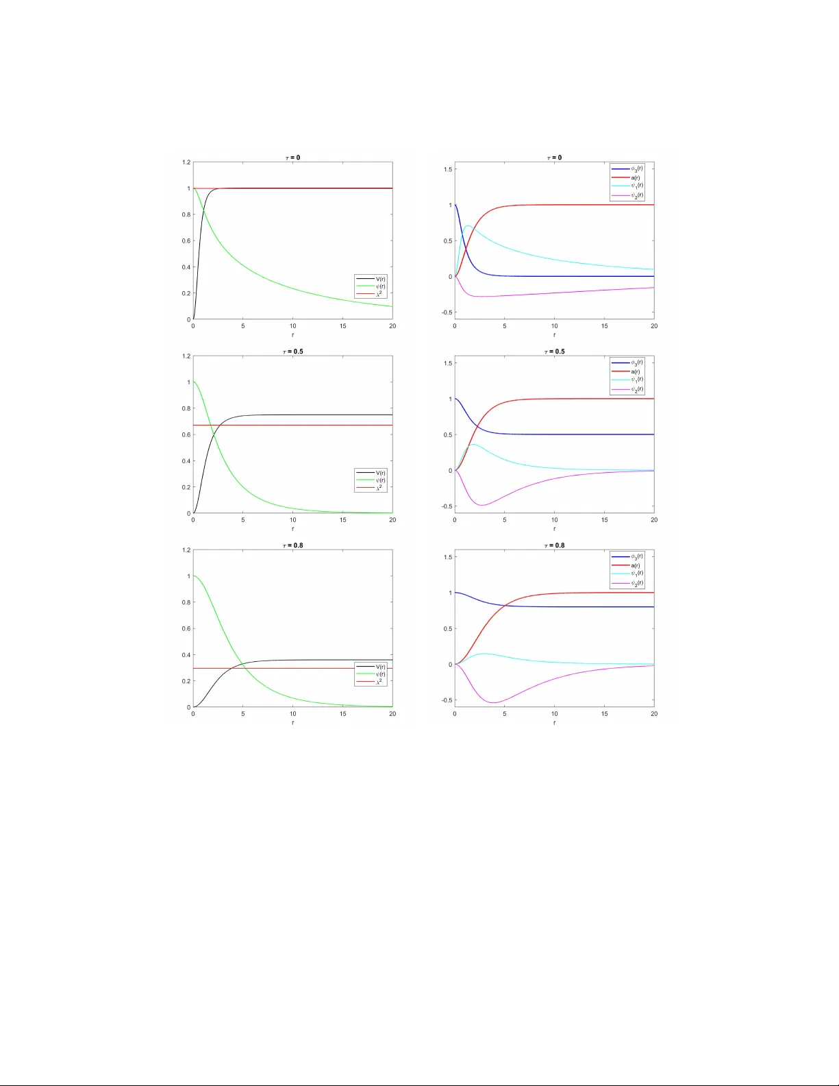
SHAPE MODES OF C P 1 V OR TICES NORA GA VREA 1 , DEREK HARLAND 2 AND MAR TIN SPEIGHT 3 Abstract. In this pap er w e inv estigate the existence of in ternal mo des of vortices in the gauged C P 1 sigma mo del. W e develop a clean geometric formalism that highlights the sym- metries of the Jacobi op erator, obtained from the second v ariation of the energy functional. The formalism and subsequent results fundamentally rely on the Bogomol’nyi decomp osi- tion of the energy functional, and can therefore be extended to other mo dels with suc h a decomp osition. W e pro ve the existence of at least one shape mode for a general C P 1 v ortex solution on R 2 , and find n umerically the shap e modes and corresp onding frequen- cies of a radially symmetric v ortex. A surprising result is that the shap e mo de eigenv alues are very close to the scattering threshold, suggesting weakly b ound shap e mo des could b e c haracteristic of the C P 1 mo del. 1. Intr oduction The gauged C P 1 sigma model (also kno wn as the gauged O (3) sigma mo del) w as o riginally dev elop ed b y Schroers [ 22 ]. It breaks the scale inv ariance of the pure C P 1 sigma model b y gauging a U (1) symmetry . After including a suitable p oten tial term, the mo del admits soliton solutions whic h provide minima of the associated energy functional within their homotop y class. They are conv en tionally called BPS as they arise as solutions of a first order PDE system obtained from a Bogomol’n yi-type argumen t [ 22 , 21 ]. This mo del and the ab elian Higgs mo del ha v e some similarities, for example the U (1) symmetry of the fields and the fact that their solutions carry a quan tized magnetic flux which mak es them top ologically stable. Solitons in b oth mo dels are referred to as vortices. In the con text of the ab elian Higgs mo del, vortices hav e b een studied from different p er- sp ectiv es and hav e b ecome relev an t in the study of b oth cosmology and sup erconductivit y . In cosmology , they describ e large-scale cosmic strings whic h lead to structure formation due to lo cal concentrations of energy [ 26 ]. In the Ginzburg-Landau theory of sup erconductivity , they describe magnetic flux tub es o ccurring in a t yp e-I I superconducting material after it is co oled do wn b elo w its critical temp erature and a magnetic field is applied [ 1 ]. Similar applications ha ve b een discov ered for the C P 1 v ortices. In [ 31 ], Y ang has shown how to construct C P 1 v ortices and anti-v ortices coupled to gravit y , representing cosmic strings and an ti-strings with opposite magnetic c harges. The C P 1 mo del has also b een prop osed to mo del the competition b etw een superconducting phases, due to its target space C P 1 ∼ = S 2 whic h comes with an additional constraint, allowing competition b et w een a sup erconducting comp onen t and a charge density w av e comp onent [ 25 , 16 ]. Date : March 25, 2026. 1 2 NORA GA VREA 1 , DEREK HARLAND 2 AND MAR TIN SPEIGHT 3 The gauged C P 1 mo del has tw o in teresting new features with no counterpart in the ab elian Higgs mo del. First it carries an extra parameter τ ∈ ( − 1 , 1), the heigh t of the v acuum manifold on S 2 . (The analogous parameter in the ab elian Higgs mo del can b e scaled a wa y .) This parameter affects the size and energy of vortices non trivially . Second, due to its compact target space, the C P 1 mo del exhibits t wo different types of vortices. In general, v ortex p ositions are the p oin ts in ph ysical space Σ that are mapp ed by the Higgs field ϕ to a fixed p oint of the action of the gauge group U (1) on the target space. In the ab elian Higgs mo del, the target space C has only one fixed p oint, the origin, so there is only one sp ecies of vortex. In the gauged C P 1 mo del, the target space S 2 has tw o fixed p oints whic h we ma y take, without loss of generalit y , to b e the ± n = (0 , 0 , ± 1), hence t w o distinct sp ecies of v ortex. These ma y generically co exist. Finite energy field configurations carry a pair of in teger v alued top ological inv arian ts, the num b ers k + , k − of preimages of these fixed points coun ted with orien tation and m ultiplicit y . Ev ery static energy minimizer in the ( k + , k − ) class defines a disjoint pair of effectiv e divisors on Σ of degrees k + and k − consisting of the preimages D + = ϕ − 1 ( n ) and D − = ϕ − 1 ( − n ). D + ∩ D − = ∅ since no p oin t can b e mapped sim ultaneously to b oth n and − n . Conv ersely , given a disjoint pair of effective divisors D + , D − of degrees ( k + , k − ) there is a static v ortex in the degree ( k + , k − ) class, unique up to gauge, with ϕ − 1 ( ± n ) = D ± . This was prov ed on Σ = R 2 b y Y ang in the symmetric case τ = 0 [ 30 ] and Han for general τ in [ 15 ]. On a compact Riemann surface Σ (of sufficien tly large area) this was prov ed by Sibner, Sibner and Y ang in the sp ecial case τ = 0 in [ 23 ], and in the case of general τ by Garcia Lara [ 14 ]. The space of all these ( k + , k − ) v ortex solutions mo dulo gauge equiv alence is called the mo duli space, which is a generically non-compact complex manifold of dimension k + + k − . The mo duli space has a natural Riemannian metric whose geodesic flo w mo dels the dynamics of slo wly mo ving vortices. A detailed analysis of the geometry of the mo duli space of C P 1 v ortices is given in [ 21 ]. Our fo cus in this pap er is the p erturbative mo des around a BPS v ortex solution, along with the frequency sp ectrum of these modes. They solve an eigen v alue problem of a certain elliptic op erator, arising from the second v ariation of the energy functional of the mo del. Quan tum mec hanically , they can b e interpreted as particle states: they can b e either b ound states (particles trapp ed in the core of the vortex) or un b ound states (particles scattering with the v ortex). Bound states hav e L 2 normalizable eigenfunctions, while scattering states do not. By a shap e mo de, we will mean a b ound state with strictly p ositive eigen v alue. (Bound mo des with eigen v alue 0 corresp ond to perturbations tangen t to the space of static solutions; all such mo des are generated by mo ving the vortex p ositions, or b y gauge transformations.) In classical dynamics, shap e mo des corresp ond to spatially lo calized oscillatory motions of the time dep endent field equations linearized ab out the static v ortex. Their existence, frequency and degeneracy are kno wn to hav e profound effects on the lo w energy scattering of ab elian Higgs vortices [ 3 , 4 , 8 , 17 , 20 ] and they hav e b een intensiv ely in v estigated in that mo del [ 5 , 6 , 10 ] by numerical means. But to date the are no rigorous analytic existence results for shap e mo des, either in the ab elian Higgs mo del or the gauged C P 1 mo del. SHAPE MODES OF C P 1 V OR TICES 3 In this pap er, w e in v estigate the existence of shap e mo des of vortices in the C P 1 mo del, fo cusing on the case Σ = R 2 . Rather than follo w the supersymmetry argumen t developed in [ 6 ] for radially symmetric abelian Higgs v ortices, w e develop a new formalism whic h allo ws for a cleaner treatmen t of the second v ariation of the energy functional as well as the eigen v alue problem giving rise to the internal mo des, w orking initially on a general surface Σ, and later sp ecializing to R 2 . This formalism fundamentally exploits the Bogomol’n yi energy decomp osition, hence in principle it can b e applied to an y mo del with this prop erty . It can b e easily applied to vortices in the abelian Higgs mo del with sligh t mo difications, and it could also b e applied to other t yp es of top ological solitons (such as monop oles or lumps). W e presen t this formalism and its implications in Section 3, where we pro v e the existence of at least one shap e mo de for a general C P 1 v ortex solution on Σ = R 2 , whic h is the main result of this paper. In Section 4, w e fo cus on the radially symmetric case with v ortices coincident at the origin and use our previous results to compute the shap e mo des n umerically . W e find that for a charge one v ortex, the shape mo de eigen v alue is v ery close to the scattering threshold, suggesting that b ound states in the C P 1 mo del are only weakly b ound. 2. The gauged C P 1 sigma model 2.1. The energy functional. Let Σ b e an orien ted Riemannian surface, and P → Σ a principal U (1)-bundle equipp ed with a connexion A . Let ϕ b e a section of the associated bundle P × ρ M → Σ, where M is the target manifold, and ρ is a Hamiltonian action of U (1) on M . In this paper w e consider Σ = R 2 and M = C P 1 whic h we iden tify as S 2 with the round metric. The action of U (1) on M = S 2 is represen ted b y rotations about the z -axis. W e will often adhere to the notation Σ, b efore w e sp ecialize our results to the particular case Σ = R 2 . In this later case, P is trivial and the Higgs field is a function ϕ : R 2 → S 2 . W e are interested in finding pairs ( A, ϕ ) which are global minimizers of the energy func- tional E [ ϕ , A ] = 1 2 Z Σ  | F | 2 + | D ϕ | 2 + | τ − n · ϕ | 2  , (2.1) where n = (0 , 0 , 1) is the constan t unit v ector p oin ting in the z -direction, F = dA is the curv ature of the connexion, and D ϕ = d ϕ − A n × ϕ is the cov arian t deriv ativ e in a local trivialization of P × ρ M . The parameter τ ∈ ( − 1 , 1) in the p oten tial U ( ϕ ) = ( τ − n · ϕ ) 2 defines the v acuum manifold, where the potential attains its minim um v alue equal to zero. (The case τ = ± 1 is somewhat pathological, and will not b e considered here.) F or the non-compact case Σ = R 2 , finite energy solutions require the follo wing b oundary conditions: lim | x |→∞ F = 0 , lim | x |→∞ D ϕ = 0 , lim | x |→∞ n · ϕ = τ . (2.2) 4 NORA GA VREA 1 , DEREK HARLAND 2 AND MAR TIN SPEIGHT 3 2.2. Gauge transformations. The energy functional ( 2.1 ) is in v arian t under the follo wing lo cal gauge transformations ϕ 7→ R ( θ ) ϕ A 7→ A + dθ, where θ : Σ → R and R ( θ ) ∈ S O (3) represen ts the rotation with angle θ ab out the z -axis R ( θ ) =   cos θ − sin θ 0 sin θ cos θ 0 0 0 1   . 2.3. The Bogomol’n yi equations. The energy functional admits a Bogomol’nyi-t ype de- comp osition, whic h results from completing the square inside the energy functional: E [ ϕ , A ] = 1 2 Z Σ  1 2 | D ϕ − ∗ ϕ × D ϕ | 2 + |∗ F + ( τ − n · ϕ ) | 2  (2.3) + Z Σ  1 2 D ϕ · ϕ × D ϕ − ( τ − n · ϕ ) F  . It can b e shown [ 21 ] that the cross term integrates to Z Σ  1 2 D ϕ · ϕ × D ϕ − ( τ − n · ϕ ) F  = 2 π (1 − τ ) k + + 2 π (1 + τ ) k − , under the assumption that F , D ϕ and n · ϕ decay sufficien tly rapidly on the boundary of Σ. The n um b ers k + and k − are in tegers enco ding the n um b er of North v ortices and South an ti-v ortices on Σ, respectively: the pre-image of the North p ole under ϕ is a set of k + p oin ts on Σ, represen ting the locations of the North v ortices, and the pre-image of the South p ole under ϕ is a set of k − p oin ts on Σ, representing the lo cations of the South an ti-v ortices. These (an ti)-v ortices are top ologically distinct, and their co-existence w as established b y Y ang [ 31 ]. The difference betw een v ortices and anti-v ortices arises from the fact that lo cal coordinate systems in the neigh b ourho o ds of the North and South p oles hav e opp osite orientations. Th us, the field winds around the v acuum manifold k + times in an ticlo ckwise direction, corresp onding to the contribution of the North vortices, and k − times in clo c kwise direction, corresp onding to the con tribution of the South an ti-v ortices. These windings are also related to the total magnetic flux through the surface [ 25 ], which is quantized and can b e computed 1 2 π Z Σ F = k + − k − . F rom the ab ov e Bogomol’nyi argumen t, w e conclude the energy is bounded below by the top ological inv ariant giv en b y the in tegration of the cross terms, and the inequality is saturated when the first order Bogomol’nyi equations hold D ϕ = ∗ ϕ × D ϕ (2.4) ∗ F = − ( τ − n · ϕ ) , (2.5) SHAPE MODES OF C P 1 V OR TICES 5 with solutions ( A, ϕ ) b eing conv en tionally called BPS solutions. It has b een sho wn that, up to gauge equiv alence, BPS configurations are determined b y the pair of divisors ( D + , D − ) with degrees ( k + , k − ) on Σ, sp ecifying the lo cations of the v ortices and anti-v ortices, resp ec- tiv ely , including their algebraic m ultiplicities [ 21 , 30 ]. 3. Shape modes of a C P 1 v or tex solution Recall the shape modes represen t the perturbative mo des around a BPS vortex solution. They are eigenmo des of the second order elliptic operator obtained from the second v ariation of the energy functional ( 2.1 ), with p ositiv e eigen v alue. They offer extensive information ab out the dynamics of excited vortices near the critical BPS point in the mo duli space. Suc h dynamics is ric h and complicated, and has b een widely studied recently in the context of the Abelian-Higgs mo del [ 4 , 7 , 8 , 17 ], rev ealing surprising phenomena, suc h as for example the existence of sp ectral walls [ 9 ]. T o inv estigate shap e mo des in the context of the C P 1 mo del, we m ust first find the second v ariation of the energy functional ( 2.1 ) around a BPS solution ( ϕ , A ). It is helpful to w ork initially on a general surface Σ, and later set Σ = R 2 . Throughout w e assume that P is trivial. W e will start b y computing the first v ariation and defining some new op erators, as this establishes a go o d starting point for the second v ariation whose calculation is more computationally difficult. 3.1. The first v ariation. Let ( ϕ s , A s ) be a 1-parameter v ariation of the BPS solution ( ϕ 0 , A 0 ) = ( ϕ , A ). This generates the infinitesimal p erturbation d ds     s =0 ϕ s ( x ) = η ( x ) , d ds     s =0 A s ( x ) = α ( x ) . W e will consider the energy functional written in Bogomol’n yi form, whic h will later enable us to write the second v ariation op erator as a comp osition of tw o first order op erators. This approac h b ecomes v ery helpful once we try to prov e existence of and construct the shap e mo des. W e hav e the energy E [ ϕ , A ] = 1 4 ∥ D ϕ − ∗ ϕ × D ϕ ∥ 2 L 2 + 1 2 ∥ ∗ F + ( τ − n · ϕ ) ∥ 2 L 2 + E 0 , where E 0 = 2 π (1 − τ ) k + + 2 π (1 + τ ) k − , and the L 2 inner pro duct is given b y ⟨ α, β ⟩ L 2 = Z Σ α ∧ ∗ β . By defining the op erator B og : C ∞  Σ , S 2  ⊕ Γ( T ∗ Σ) → Γ( T ∗ Σ ⊗ ϕ ∗ T S 2 ) ⊕ C ∞ (Σ)  ϕ A  7→    1 √ 2 ( D ϕ − ∗ ϕ × D ϕ ) ∗ F + ( τ − n · ϕ )    , 6 NORA GA VREA 1 , DEREK HARLAND 2 AND MAR TIN SPEIGHT 3 w e can re-write the energy more compactly as E [ ϕ , A ] = 1 2 ⟨ B og ( ϕ , A ) , B og ( ϕ , A ) ⟩ L 2 + E 0 . (3.1) Then the first v ariation of the energy is given by d ds     s =0 E [ ϕ s , A s ] =  d ds     s =0 B og ( ϕ s , A s ) , B og ( ϕ s , A s )  L 2 = ⟨ B ξ , B og ( ϕ , A ) ⟩ L 2 , where ξ =  η α  and B is the differential of the map B og at ( ϕ, A ): B : Γ( ϕ ∗ T S 2 ) ⊕ Γ( T ∗ Σ) → Γ( T ∗ Σ ⊗ ϕ ∗ T S 2 ) ⊕ C ∞ (Σ) ξ =  η α  7→    1 √ 2 ( D η − α n × ϕ − ∗ η × D ϕ − ∗ ϕ × ( D η − α n × ϕ )) ∗ dα − n · η    . The domain of this op erator will o ccur frequen tly in the sequel, so it is useful to give it a name. Since it is the space of linear p erturbations ab out the static vortex ( ϕ , A ) we call it P E RT := Γ( ϕ ∗ T S 2 ) ⊕ Γ( T ∗ Σ) (3.2) T o rewrite the op erator B more compactly and to ensure an easier calculation for the second v ariation in the next subsection, it is helpful to define the following linear op erators L ϕ : Γ( T ∗ Σ ⊗ ϕ ∗ T S 2 ) → Γ( T ∗ Σ ⊗ ϕ ∗ T S 2 ) η 7→ 1 √ 2 ( η − ϕ × ∗ η ) (3.3) P ϕ : Γ( T ∗ Σ ⊗ R 3 ) → Γ( T ∗ Σ ⊗ ϕ ∗ T S 2 ) u 7→ u − ( u · ϕ ) ϕ . (3.4) One easily v erifies that L ϕ ◦ L ϕ = √ 2 L ϕ (3.5) P ϕ ◦ P ϕ = P ϕ (3.6) [ L ϕ , ∗ ] = 0 (3.7) [ L ϕ , P ϕ ] = 0 (3.8) L † ϕ = L ϕ (3.9) P † ϕ = P ϕ , (3.10) where the “dagger” sup erscript denotes the L 2 -adjoin t of the resp ective op erator, and B  η α  = L ϕ ◦ P ϕ ( D η − α n × ϕ ) ∗ dα − n · η ! . (3.11) SHAPE MODES OF C P 1 V OR TICES 7 3.2. The second v ariation. Let ( ϕ s,t , A s,t ) b e a 2-parameter v ariation of the BPS solution ( ϕ 0 , 0 , A 0 , 0 ) = ( ϕ , A ). This generates the infinitesimal p erturbations ∂ ∂ s     s =0 ϕ s,t ( x ) = η t ( x ) , ∂ ∂ s     s =0 A s,t ( x ) = α t ( x ) ∂ ∂ t     s = t =0 ϕ s,t ( x ) = ˜ η ( x ) , ∂ ∂ t     s = t =0 A s,t ( x ) = ˜ α ( x ) . Let ξ = ( η 0 , α 0 ) and ˜ ξ = ( ˜ η , ˜ α ) The second v ariation of the energy functional around a BPS solution is then given by ∂ ∂ t     t =0 ∂ ∂ s     s =0 E [ ϕ s,t , A s,t ] =  ∂ ∂ s     s =0 B og ( ϕ s,t , A s,t ) , ∂ ∂ t     t =0 B og ( ϕ s,t , A s,t )  L 2 = D B ξ , B ˜ ξ E L 2 = D ξ , B † B ˜ ξ E L 2 , (3.12) where B † : Γ( T ∗ Σ ⊗ ϕ ∗ T S 2 ) ⊕ C ∞ (Σ) → P E RT  χ 1 χ 2  7→ P ϕ ( − ∗ D ∗ L ϕ ( χ 1 ) − n χ 2 ) − ∗ dχ 2 − ( n × ϕ ) · L ϕ ( χ 1 ) ! (3.13) is the L 2 -adjoin t of B expressed in ( 3.11 ). Its calculation follo ws quic kly b y using the prop erties listed in ( 3.5 )-( 3.10 ). Recall that the p erturbation η comes with the constraint η ( x ) ∈ T ϕ ( x ) S 2 , and hence w e should b e careful with handling inner pro ducts of the t yp e ⟨ η , ·⟩ L 2 when deriving expression ( 3.13 ), since only the terms p erp endicular to ϕ bring a contribution, as the ones parallel to ϕ equate to zero when tak en in the inner pro duct with η . T o rule out the o ccurence of suc h extraneous terms, w e note ⟨ η , ·⟩ L 2 = ⟨ η , P ϕ ( · ) ⟩ L 2 . Note from ( 3.12 ) we can no w identify the second v ariation operator J , called the Jacobi op erator, with J = B † B . This decomp osition reinforces more ob viously that J is a p ositive semi-definite self-adjoin t op erator. An imp ortant observ ation is that we w ere able to decomp ose the Jacobi op erator into a pro duct of t w o first order op erators, one of which is the L 2 -adjoin t of the other, simply due to the fact that the energy functional admits a Bogomol’n yi argumen t. Hence this represen ts a general prop ert y of this type of mo dels. 3.3. Zero mo des and the orthogonal gauge condition. Recall the energy functional ( 2.1 ) is inv arian t under the gauge transformations presen ted in subsection 2.2. Therefore, p erturbations of the fields represen ted by infinitesimal gauge transformations lea v e the Bo- gomol’n yi equations inv ariant, and lie in the k ernel of the op erator B . 8 NORA GA VREA 1 , DEREK HARLAND 2 AND MAR TIN SPEIGHT 3 Let us denote b y G the map whic h assigns to a smo oth real function on Σ the infinitesimal gauge transformation that it generates: G : C ∞ (Σ) → P E RT χ 7→ ( χ n × ϕ , dχ ) . (3.14) As we ha v e just observ ed, BG = 0, that is, infinitesimal gauge transformations lie in the k ernel of B . If we wish to contruct the tangent space to the vortex moduli space at (the gauge equiv alence class of ) ( ϕ , A ), we should keep only those vectors in k er B which are L 2 orthogonal to all suc h gauge transformations, i.e. ⟨ G ( χ ) , ( η , α ) ⟩ L 2 = 0 for all χ . Clearly this is equiv alent to G † ( η , α ) = 0 (3.15) where G † : P E RT → C ∞ (Σ) ( η , α ) 7→ − ∗ d ∗ α + η · ( n × ϕ ) (3.16) is the L 2 adjoin t of G . Hence T [( ϕ ,A )] M , the tangen t space of the mo duli space M at the p oin t ([ ϕ , A )], is precisely the k ernel of the extended op erator B G : = B ⊕ G † : P E RT → B O G (3.17) whose co domain w e hav e denoted B O G := Γ( T ∗ Σ ⊗ ϕ ∗ T S 2 ) ⊕ C ∞ (Σ) ⊕ C ∞ (Σ) . The L 2 -adjoin t of B G is B G † : B O G → P E RT   χ 1 χ 2 χ 3   7→ P ϕ ( − ∗ D ∗ L ϕ ( χ 1 ) − n χ 2 ) + n × ϕ χ 3 − ∗ dχ 2 − ( n × ϕ ) · L ϕ ( χ 1 ) + dχ 3 ! , (3.18) using the prop erties ( 3.5 )-( 3.10 ). Since J = B † B , it follo ws immediately that JG = 0 , G † J = 0 . (3.19) Hence, every eigenmo de of J not in its kernel automatically satisfies the gauge orthogonalit y condition ( 3.15 ). 3.4. The extended Jacobi op erator. W e can no w define the extended Jacobi op erator b y J G : = B G † B G = B † B + GG † = J + GG † : P E RT → P E RT . (3.20) W e will prov e shortly that J and J G ha v e the same eigenv alue sp ectrum. SHAPE MODES OF C P 1 V OR TICES 9 Analyzing the structure of the op erators B G and B G † , it is helpful to define the L 2 isome- tries S 1 : P E RT → P E RT  η α  7→  ϕ × η ∗ α  (3.21) S 2 : B O G → B O G   χ 1 χ 2 χ 3   7→   ∗ χ 1 − χ 3 χ 2   . (3.22) The follo wing lemma concerns the prop erties of the maps ( 3.21 ) and ( 3.22 ) and the symme- tries of the op erators J G and B G B G † . Lemma 3.1. The maps S 1 and S 2 satisfy the fol lowing pr op erties S 1 ◦ S 1 = − id P E RT (3.23) S 2 ◦ S 2 = − id BO G (3.24) S † 1 = − S 1 (3.25) S † 2 = − S 2 (3.26) G † S 1 G = 0 (3.27) F urthermor e,  J G , S 1  = 0 and  B G B G † , S 2  = 0 , i.e. they r epr esent symmetries of the op er- ators J G and B G B G † , r esp e ctively. Pr o of . F rom the definitions of the t w o maps given in ( 3.21 ) and ( 3.22 ) it is immediate to c hec k that the prop erties ( 3.23 )-( 3.26 ) hold. T o prov e ( 3.27 ) we compute directly by using the definitions ( 3.14 ), ( 3.16 ), ( 3.21 ) G † S 1 G χ = G †  ϕ × ( n × ϕ ) χ ∗ dχ  = − ∗ d ∗ ( ∗ dχ ) + [ ϕ × ( n × ϕ ) χ ] · ( n × ϕ ) = 0 . F rom the expressions ( 3.17 ) and ( 3.18 ) w e can easily chec k that B G S 1 = S 2 B G (3.28) B G † S 2 = S 1 B G † , (3.29) where the second equation can also b e obtained by taking the L 2 -adjoin t of the first one. Applying B G † to ( 3.28 ) w e obtain B G † B G S 1 = B G † S 2 B G = S 1 B G † B G , where in the second equality w e used ( 3.29 ). Hence the op erators J G and S 1 comm ute J G S 1 = S 1 J G , (3.30) 10 NORA GA VREA 1 , DEREK HARLAND 2 AND MAR TIN SPEIGHT 3 whic h is equiv alen t to sa ying that S 1 is a symmetry of the op erator J G . Similarly , applying B G to ( 3.29 ) yields B G B G † S 2 = S 2 B G B G † . (3.31) □ R emarks. (1) The map S 1 is an isometry of P E RT (with respect to its natural L 2 inner pro duct) whic h squares to − id . Hence it ma y naturally b e in terpreted as an almost complex structure on P E RT . Its restriction to ker B G is precisely the natural almost complex structure on the v ortex mo duli space. (2) The ab ov e Lemma implies that if ξ is an eigenmode of J G with eigen v alue λ 2 , then so is S 1 ξ , and similarly if χ is an eigenmo de of B G B G † with eigen v alue λ 2 , then so is S 2 χ . So eigenmo des of J G come in degenerate pairs. (3) W e also notice that if χ is an eigenmo de of B G B G † with eigenv alue λ 2 , then B G † χ (if non-zero) is an eigenmo de of J G with the same eigenv alue. This observ ation will turn out to be crucial later when w e compute the shap e mo des, as the op erator B G B G † allo ws for the decoupling of the PDE system obtained in the eigenv alue problem. (4) Finally , observe that if ξ ∈ ker J G , then 0 =  ξ , J G ξ  L 2 =  B G ξ , B G ξ  L 2 =   B G ξ   2 L 2 , implying B G ξ = 0. Hence ker J G = k er B G , and similarly k er B G B G † = k er B G † . No w that w e are equipp ed with these new op erators, w e show that this form ulation allows for an elegan t and quick computation of a vortex shap e mo de. Theorem 3.2. If ψ : Σ → R is an L 2 eigenfunction of the Schr¨ odinger op er ator L = ∆ + | n × ϕ | 2 (3.32) then S 1 G ψ is an L 2 -inte gr able eigenmo de of J with the same eigenvalue. Her e ∆ = − ∗ d ∗ d denotes the L aplac e-Beltr ami op er ator on Σ . Pr o of . First observe that L = G † G . Applying G to the left, w e observe that if Lψ = λ 2 ψ , then GG † ( G ψ ) = λ 2 G ψ and k er G = 0 b y its definition ( 3.14 ), so G ψ is an eigenmode of GG † with the same eigen v alue. No w JG = 0 since, for all χ ∈ C ∞ (Σ), G ( χ ) is an infinitesimal gauge transformation, all of whic h lie in the kernel of J by the gauge inv ariance of the energy functional. Hence J G G ψ = ( J + GG † ) G ψ = GG † G ψ = λ 2 G ψ , that is, G ψ is an eigenmo de of J G with eigen v alue λ 2 . SHAPE MODES OF C P 1 V OR TICES 11 By the symmetry we prov ed in Lemma 3.1 , we deduce that S 1 G ψ is also an eigenmo de of J G . Then we hav e JS 1 G ψ = ( J G − GG † ) S 1 G ψ = J G ( S 1 G ψ ) = λ 2 S 1 G ψ , b y ( 3.27 ) pro v ed in Lemma 3.1 . W e therefore deduce that S 1 G ψ is also an eigenmo de of J . The L 2 -in tegrabilit y part of the theorem follows quickly by noticing | S 1 G ψ | 2 L 2 = ⟨ S 1 G ψ , S 1 G ψ ⟩ L 2 = D ψ , G † S † 1 S 1 G ψ E L 2 = λ 2 ⟨ ψ , ψ ⟩ L 2 < ∞ , where we used ( 3.25 ), ( 3.23 ) and G † G ψ = λ 2 ψ . Hence if ψ is L 2 -in tegrable, then so is S 1 G ψ . □ R emarks. (1) Since the p otential | n × ϕ | 2 in the Sc hr¨ odinger op erator is non-negative and v anishes only on the divisors D ± , an y L 2 eigenmo de constructed in this w ay must hav e λ 2 > 0, and so is a shap e mo de. (2) The ab o v e prop osition reveals a p o w erful and quic k metho d to construct a shap e mo de, by solving a single scalar PDE Lψ = λ 2 ψ . This is m uc h simpler than solving the eigen v alue problem for J directly (a coupled system of 5 PDEs with a constrain t). Ho w ever, there is no guarantee that this metho d will give all p ossible shap e modes. T o find all p ossible shap e mo des of a giv en v ortex solution, w e need to solv e the eigen v alue problem for the op erator J , which fails to b e elliptic. W e next sho w that the eigenv alue sp ectrum of J coincides precisely with that of J G , which is elliptic. The pro of will make use of the orthogonal decomp osition P E RT = G ∞ ⊕ G ⊥ ∞ where G ∞ = Im G is the space of infinitesimal gauge transformations and G ⊥ ∞ = ker G † is its L 2 orthogonal complemen t. Prop osition 3.3. Assume k +  = 0 or k −  = 0 . Then the op er ators J and J G = J + GG † have the same L 2 -eigenvalues, c orr esp onding to eigenmo des which ar e L 2 -inte gr able. Pr o of . W e first observe that 0 is an eigen v alue of b oth J and J G since any tangent vec- tor to M at [( ϕ , A )] is in the k ernel of b oth B and B G . It remains to sho w that J , J G ha v e the same non-zero eigen v alues. First assume ξ  = 0 is L 2 and J ξ = λ 2 ξ with λ 2  = 0. Then it follows from ( 3.19 ) that G † ξ = 0 and hence J G ξ = J ξ = λ 2 ξ . Hence ξ is an L 2 eigenmo de of J G with the same eigen v alue. Con v ersely , assume that ξ  = 0 is L 2 and J G ξ = λ 2 ξ with λ 2  = 0. Denote b y ξ = ξ g + ξ g ⊥ , where ξ g ∈ G ∞ , ξ g ⊥ ∈ G ⊥ ∞ its decomp osition in to G ∞ ⊕ G ⊥ ∞ . Then we hav e, by ( 3.19 ), J G ξ = J ξ g ⊥ + GG † ξ g = λ 2 ( ξ g + ξ g ⊥ ) , 12 NORA GA VREA 1 , DEREK HARLAND 2 AND MAR TIN SPEIGHT 3 whose comp onen ts in G ⊥ ∞ and G ∞ are GG † ξ g = λ 2 ξ g (3.33) J ξ g ⊥ = λ 2 ξ g ⊥ (3.34) resp ectiv ely . Hence, if ξ g ⊥  = 0, it is an L 2 eigenmo de of J , and the claim is established. Finally , consider the case that ξ g ⊥ = 0, so ξ = ξ g = G ( χ ) for some χ ∈ C ∞ (Σ). Then G † S 1 ξ g = G † S 1 G ( χ ) = 0 by equation ( 3.27 ), so JS 1 ξ g = J G S 1 ξ g = S 1 J G ξ g = λ 2 S 1 ξ g , b y Lemma 3.1 . S 1 is an L 2 isometry , so S 1 ξ g is an L 2 eigenmo de of J with eigen v alue λ 2 , whic h completes the pro of. □ Our next existence result builds on Theorem 3.2 . Theorem 3.4. L et ( ϕ , A ) b e a solution to the Bo gomol’nyi e quations on Σ = R 2 with nonempty p air of divisors ( D + , D − ) . Then ther e exists a b ound state of the BPS C P 1 vortex if either of the fol lowing holds • k − = | D − | = 0 and τ ∈ (0 , 1) • k + = | D + | = 0 and τ ∈ ( − 1 , 0) • τ = 0 . Pr o of . In Theorem 3.2 , we prov ed that if ψ is an eigenmo de of G † G , then S 1 G ψ is an eigenmo de of J . Hence if we can find a b ound state of the Sc hr¨ odinger op erator ( 3.32 ), then S 1 G ψ represen ts a b ound state of the vortex solution. W e can re-write the eigenv alue problem for ( 3.32 ) as −∇ 2 ψ + V ψ = E ψ , (3.35) where E = λ 2 − (1 − τ 2 ) and V = | n × ϕ | 2 − (1 − τ 2 ) = τ 2 − ( n · ϕ ) 2 . W e observe that this new p oten tial has the prop erty that lim | x |→∞ V ( x ) = lim | x |→∞ [ τ 2 − ( n · ϕ ) 2 ] = 0 , due to the b oundary conditions on ϕ . W e now use a maximum principle to prov e that V ( x ) ≤ 0 everywhere on the plane in the cases sp ecified. In order to do so, w e first pro ject stereographically from the South p ole of S 2 . This allows us to instead w ork with the complex field u = ϕ 1 + iϕ 2 1 + ϕ 3 . The Bogomol’nyi equations then transform to ˜ D 1 u = − i ˜ D 2 u ∗ dA = −  τ − 1 − | u | 2 1 + | u | 2  , SHAPE MODES OF C P 1 V OR TICES 13 where no w the cov arian t deriv ative is ˜ D u = du − iAu . Note w e can write | u | 2 = 1 − ϕ 3 1 + ϕ 3 , (3.36) and define v = ln 1 − ϕ 3 1 + ϕ 3 + ln 1 + τ 1 − τ . (3.37) Using the b oundary conditions on ϕ , w e hav e lim | x |→∞ v ( x ) = 0. Note that D + , D − are the collections of p oints in R 2 at whic h ϕ = n and − n resp ectively , so at each p ∈ D + , v ( p ) = −∞ and at eac h q ∈ D − , v ( q ) = ∞ . Com bining the tw o Bogomol’nyi equations, w e obtain the so called T aub es equation ∇ 2 v = 2 e v − 1 1 1 − τ + e v 1 + τ + 4 π X q ∈ D − δ ( q ) − 4 π X p ∈ D + δ ( p ) . (3.38) In [ 30 ], this equation w as deriv ed for the case τ = 1. In [ 15 ], it was prov en that ( 3.38 ), as a particular example of a more general T aub es-t yp e equation considered b y the author, admits a unique solution for an y parameter τ ∈ ( − 1 , 1), that this solution is smo oth aw a y from D ± and exp onen tially lo calized. W e observe that ϕ 3 ≥ τ is equiv alent to v ≤ 0. W e no w assume k − = 0, so v only has negative singularities, and τ ∈ (0 , 1). If v is not everywhere non-p ositiv e, then since lim | x |→∞ v ( x ) = 0, it must ac hiev e a maximum at some z 0 , suc h that v ( z 0 ) > 0. A t this maxim um, the Hess ian H ess ( v ( z 0 )) is negative semidefinite, hence T r ( H ess ( v ( z 0 )) ≤ 0, but the trace of the Hessian is equal ∇ 2 v , and therefore ∇ 2 v ( z 0 ) ≤ 0. Observ e that the LHS of ( 3.38 ) is non-p ositive at z 0 , while the RHS is p ositive, leading to a con tradiction. W e deduce that ϕ 3 ( x ) ≥ τ everywhere on the plane. Since τ > 0, then w e also ha v e ( ϕ 3 ) 2 ≥ τ 2 , and hence V ( x ) ≤ 0 ev erywhere on the plane. The case k + = 0 and τ ∈ ( − 1 , 0) follows from a similar argument, where no w the signs are flipp ed and w e obtain ϕ 3 ≤ τ everywhere on the plane. Since τ < 0, we reach the same conclusion that ( ϕ 3 ) 2 ≥ τ 2 , and th us again V ( x ) ≤ 0. The last case follo ws from the simple observ ation that τ = 0 implies immediately that the p otential V ( x ) = τ 2 − ( ϕ 3 ) 2 is everywhere non-p ositiv e without an y assumption on the n um b er of vortices and anti-v ortices. A simple v ariational method with a clev erly chosen test function sho ws that an y smo oth p oten tial V ( x ) in t w o dimensions ob eying V ( x ) ≤ 0 for all x ∈ R 2 , V ( x ) < 0 at some x and lim | x |→∞ V ( x ) = 0 supports at least one b ound state [ 29 ]. W e note that for a bound state w e m ust ha v e E < 0, so the eigen v alue is restricted to λ 2 < 1 − τ 2 . W e therefore conclude that there exists at least one shape mo de of the v ortex solution for each of the three cases considered. □ W e can impro v e Theorem 3.4 by extending the range of τ for which at least one b ound state exists b y using an explicit test function and a con tin uit y argument. 14 NORA GA VREA 1 , DEREK HARLAND 2 AND MAR TIN SPEIGHT 3 Theorem 3.5. L et ( ϕ , A ) b e a solution of the Bo gomol’nyi e quations on Σ = R 2 with a fixe d nonempty p air of divisors ( D + , D − ) . Then ther e exists a b ound state of the BPS C P 1 vortex if any of the fol lowing holds • k − = | D − | = 0 and τ ∈ ( − τ ∗ , 1) • k + = | D + | = 0 and τ ∈ ( − 1 , τ ∗ ) • τ ∈ ( − τ ∗ , τ ∗ ) , wher e τ ∗ ∈ (0 , 1) dep ends on the divisor p air ( D + , D − ) . Pr o of . In order to extend the range of τ , w e need to construct a test function and apply the v ariational metho d. T aking inner pro ducts on b oth sides and integrating by parts in ( 3.35 ) we can express the energy as the Ra yleigh-Ritz quotient E = ⟨ ψ , H ψ ⟩ L 2 ⟨ ψ , ψ ⟩ L 2 = 1 || ψ || 2 L 2 Z R 2  | dψ | 2 + V ( r , θ ) ψ 2  r dr dθ , (3.39) where the Hamiltonian operator is giv en b y H = L − (1 − τ 2 ) = −∇ 2 + V ( r , θ ), and ( r, θ ) are p olar co ordinates on the plane. Let E 0 b e the ground state energy of H . The v ariational metho d states that the energy of an arbitrary state is alw a ys at least E 0 . Hence if w e can find a state for which the Ra yleigh quotien t is negative, then we can infer that the true ground state energy E 0 is also negative, whic h leads to the existence of at least one b ound state. Giv en τ , consider the family of test functions ψ α,τ ( r ) = e − √ 1 − τ 2 − α 2 r , (3.40) with α 2 < 1 − τ 2 . Plugging into ( 3.39 ) we obtain the asso ciated energy E ( α, τ ) = 2 π (1 − τ 2 − α 2 ) Z R 2  1 − α 2 − ( ϕ 3 ) 2  ψ 2 α,τ r dr dθ , where recall that the p otential can b e written as V = τ 2 − ( ϕ 3 ) 2 . Let I α = Z R 2  1 − α 2 − ( ϕ 3 ) 2  ψ 2 α,τ r dr dθ , (3.41) and note that I α is finite for all α 2 < 1 − τ 2 , since lim | x |→∞ ϕ 3 ( x ) = τ and ψ α,τ is exp onen tially deca ying. F urthermore, if α 2 = 1 − τ 2 , then I √ 1 − τ 2 = Z R 2  τ 2 − ( ϕ 3 ) 2  r dr dθ is also finite due to the exp onential conv ergence of ϕ 3 to τ . Before contin uing our argumen t for extending the range of τ for which shap e mo des exist, w e first need to establish that E ( α, τ ) is contin uous in τ in a small neigh b ourho o d of τ = 0. Notice that the energy dep ends on ϕ 3 whic h itself dep ends on τ , and hence we need to SHAPE MODES OF C P 1 V OR TICES 15 establish some form of contin uit y of ϕ 3 with resp ect to τ . The following theorem, whose pro of is presented in an app endix, suffices: Theorem 3.6. Given a disjoint p air of divisors ( D + , D − ), let ( A τ , ϕ τ ) b e the solution (unique up to gauge) of the Bo gomol’nyi e quations ( 2.4 ) and ( 2.5 ) with p ar ameter τ . Then ther e exists ϵ ∈ (0 , 1) such that the map Φ : ( − ϵ, ϵ ) → L 2 ( R 2 ) τ 7→ ϕ τ 3 − τ is C 1 . In the remaining part of the proof w e will refer to ϕ 3 b y ϕ τ 3 to emphasize its dep endence on τ . A simple calculation sho ws that E ( α, τ ) = 1 − α 2 − 2 π (1 − τ 2 − α 2 ) Z R 2 ( ϕ τ 3 ) 2 ψ 2 α,τ r dr dθ . It therefore remains to pro v e that τ 7→ ϕ τ 3 ψ α,τ is contin uous in L 2 . Recalling τ 7→ Φ( τ ) = ϕ τ 3 − τ is con tin uous on τ in a small neighbourho o d of τ = 0 by Theorem 3.6 , w e can rewrite Z R 2 ( ϕ τ 3 ) 2 ψ 2 α,τ d 2 x = Z R 2 ( ϕ τ 3 − τ ) 2 ψ 2 α,τ d 2 x + 2 τ Z R 2 ϕ τ 3 ψ 2 α,τ d 2 x − τ 2 Z R 2 ψ 2 α,τ d 2 x = Z R 2 Φ( τ ) 2 ψ 2 α,τ d 2 x + 2 τ Z R 2 Φ( τ ) ψ 2 α,τ d 2 x + τ 2 Z R 2 ψ 2 α,τ d 2 x (3.42) Note τ 2 Z R 2 ψ 2 α,τ d 2 x = τ 2 π 2(1 − τ 2 − α 2 ) is obviously con tin uous in τ in a small neigh b ourho o d of τ = 0. Now w e deal with the remaining t w o integrals. Consider τ , τ 0 ∈ ( − ϵ, ϵ ), where 0 < ϵ ≪ 1. Then w e hav e     Z R 2 Φ( τ ) ψ 2 α,τ d 2 x − Z R 2 Φ( τ 0 ) ψ 2 α,τ 0 d 2 x     =     Z R 2 (Φ( τ ) − Φ( τ 0 )) ψ 2 α,τ d 2 x + Z R 2 Φ( τ 0 )( ψ 2 α,τ − ψ 2 α,τ 0 ) d 2 x     ≤   ⟨ Φ( τ ) − Φ( τ 0 ) , ψ 2 α,τ ⟩ L 2   + |⟨ ψ α,τ − ψ α,τ 0 , Φ( τ 0 )( ψ α,τ + ψ α,τ 0 ) ⟩ L 2 | ≤ ∥ Φ( τ ) − Φ( τ 0 ) ∥ L 2 ∥ ψ 2 α,τ ∥ L 2 + ∥ ψ α,τ − ψ α,τ 0 ∥ L 2 ∥ Φ( τ 0 )( ψ α,τ + ψ α,τ 0 ) ∥ L 2 → 0 as τ → τ 0 (3.43) since Φ and τ 7→ ψ α,τ are L 2 − con tin uous in a small neighourho o d of τ = 0, and the other L 2 − norms are finite due to their integrands’ exp onential deca y . In a v ery similar manner we also prov e that τ 7→ R R 2 Φ( τ ) 2 ψ 2 α,τ d 2 x is contin uous in a small neigh b ourho o d around τ = 0. This completes the pro of that τ 7→ R R 2 ( ϕ τ 3 ) 2 ψ 2 α,τ is con tin uous, 16 NORA GA VREA 1 , DEREK HARLAND 2 AND MAR TIN SPEIGHT 3 and therefore w e deduce that E ( α , τ ) is con tin uous on τ in a small neigh b ourho o d around τ = 0. W e can now use this fact to prov e the statemen t of the theorem. Assume τ = 0 and k ± are not both 0. Then ob viously I 1 < 0. Since I α dep ends con tin uously on α (the α dep endence of the integrand is explicit through p olynomial and exp onential functions), there exists α ∗ < 1 suc h that I α ∗ < 0, and hence E ( α ∗ , 0) < 0. Since E ( α ∗ , τ ) is con tin uous in τ , w e deduce there exists a small neighbourho o d τ ∈ ( − τ ∗ , τ ∗ ) for which E ( α ∗ , τ ) < 0, and hence a b ound state exists. Notice this argument depends on the solution ( ϕ , A ), and therefore τ ∗ dep ends on the lo cations of the (anti-)v ortices, information which is enco ded in the divisor pair ( D + , D − ). W e can now easily extend this argument to the cases where k − = 0 or k + = 0. The ab o ve argumen t prov ed there exists a b ound state for any k ± if τ ∈ ( − τ ∗ , τ ∗ ), so in particular w e can set k − = 0. F rom Theorem ( 3.4 ), a b ound state exists for k − = 0 and τ ∈ (0 , 1). Com bining these t wo results we deduce there exists a b ound state when k − = 0 and τ ∈ ( − τ ∗ , 1). Similarly w e deduce we ha ve a b ound state when k + = 0 and τ ∈ ( − 1 , τ ∗ ). □ 4. Radiall y symmetric v or tices In this section, w e apply our previous results in the particular case where w e assume radial symmetry and all vortices are concen trated at the origin. The Bogomol’nyi equations reduce to t w o coupled ODEs. W e compute the shape mo des n umerically b y solving the Bogomol’n yi equations and the ODE reduced from ( 3.35 ) together as a system. 4.1. Symmetry reduction on Σ = R 2 . If we ass ume radial symmetry , the lo cations of all (an ti)-v ortices are constrained to the origin of R 2 . Therefore, w e can only hav e either N North v ortices ( k + = N , k − = 0) or N South an ti-v ortices ( k + = 0, k − = N ). Cho osing the former case, as the latter follo ws in a v ery similar manner, w e lo ok for solutions using the hedgehog ansatz ϕ ( x ) = (sin f ( r ) cos N θ, sin f ( r ) sin N θ, cos f ( r )) (4.1) A = N a ( r ) dθ , (4.2) where ( r , θ ) are polar co ordinates on the plane. Plugging these in the Bogomol’n yi equations, they reduce to a system of first order ODEs for a ( r ) and f ( r ): f ′ = N r (1 − a ) sin f (4.3) a ′ = − r N ( τ − cos f ) . (4.4) The condition ϕ (0) = (0 , 0 , 1) that all vortices are superp osed at the origin implies that f (0) = 0. F urthermore, regularity of the gauge field at the origin imp oses a (0) = 0, and the b oundary conditions w e set b efore reduce to lim r →∞ a ′ ( r ) = 0, lim r →∞ a ( r ) = 1, lim r →∞ cos f ( r ) = τ . SHAPE MODES OF C P 1 V OR TICES 17 Hence, as r → ∞ , ϕ approaches the v acuum manifold given b y ( √ 1 − τ 2 cos N θ , √ 1 − τ 2 sin N θ , τ ) . 4.2. Asymptotic b ehaviour and magnetic flux. By lo oking at the asymptotic b ehaviour of ( 4.3 ) and ( 4.4 ) in the t w o regimes r → 0, r → ∞ , we can find analytic appro ximations for the functions f ( r ), a ( r ). • As r → 0, w e find a ( r ) ≈ r 2 2 N (1 − τ ) (4.5) f ( r ) ≈ Ar N , (4.6) where A is an arbitrary constant, and will b e used as a sho oting constan t to find the v ortex solution numerically . • As r → ∞ , w e find a ( r ) ≈ 1 − q 2 N π r K 1 ( r √ 1 − τ 2 ) (4.7) f ( r ) ≈ arccos τ − q 2 π K 0 ( r √ 1 − τ 2 ) , (4.8) where K 0 , K 1 are mo dified Bessel functions of the second kind. The constan t q represen ts the strength of the asymptotic vortex charge in the particle in tepretation of Sp eigh t [ 24 , 25 ]. These asymptotics hold in the case τ ∈ ( − 1 , 1). A quick calculation using the hedgehog ansatz sho ws that F = N a ′ ( r ) dr ∧ dθ . Hence we can directly compute the total magnetic flux Z R 2 F = 2 π N , whic h is quan tized since N is an in teger. One should note that this result dep ends crucially on our choice to restrict τ to ( − 1 , 1). If τ = ± 1, the magnetic flux is not quan tised, but it is equal to N α , where α = lim r →∞ a ( r ) [ 22 ]. 4.3. Shap e mo des of a cylindrically symmetric C P 1 N -v ortex. W e follo w the strategy giv en b y Theorem 3.2 which allows us to easily compute at least one shap e mo de of the v ortex solution by firstly solving for the eigenfunctions of the Sc hr¨ odinger op erator ( 3.32 ). T o pro ve that this strategy indeed gives us all the p ossible shap e mo des in the case of a radially symmetric N -v ortex, w e then construct the operator B G B G † in radial co ordinates, and sho w it reduces to the single PDE given by the eigenv alue problem of ( 3.32 ). In the case of radial symmetry , substituting the hedgehog ansatz ( 4.1 ) shows that the op erator ( 3.32 ) b ecomes L = ∆ + sin 2 f ( r ) . 18 NORA GA VREA 1 , DEREK HARLAND 2 AND MAR TIN SPEIGHT 3 T o find the eigenfunctions of L w e need to solv e the eigen v alue problem L Ψ = λ 2 Ψ. Moti- v ated b y the U (1) symmetry , we mak e the ansatz Ψ( r, θ ) = ψ ( r ) e ikθ , where k is an in teger. The eigen v alue problem then reduces to − ψ ′′ − 1 r ψ ′ +  k 2 r 2 + sin 2 f  ψ = λ 2 ψ , (4.9) Since the potential depends explicitly on the radial profile of the Higgs field, w e need to solve ( 4.9 ) together with ( 4.3 ) and ( 4.4 ). Theorem 3.2 show ed that the shap e mo de is then given b y S 1 G Ψ( r ) = ( n − ( n · ϕ ) ϕ ) ψ ( r ) e ikθ r ψ ′ ( r ) e ikθ dθ − i k r ψ e ikθ dr ! =  η α  . and can b e visualised in Figures 2 , 3 and 4 for the cases N = 1 , 2 , 3, and k = 0, where w e define ψ 1 ( r ) : = | η 3 | = (1 − ( ϕ 3 ) 2 ) ψ ( r ) (4.10) ψ 2 ( r ) : = r ψ ′ ( r ) . (4.11) 4.4. Shap e mo de asymptotics. By lo oking at the asymptotic b eha viour of the Schr¨ odinger equation ( 4.9 ) in the t w o regimes r → 0 and r → ∞ , w e can find analytic appro ximations for the b ound state solutions ψ ( r ). • As r → 0, w e find ψ ( r ) ≈ C 0 J k ( λr ) (4.12) where J k is a Bessel function of the first kind and C 0 is an arbitrary constan t. The ODE is linear and hence C 0 can be c hosen arbitrarily . In particular, w e can alwa ys rescale it suc h that C 0 = 1, which w e will use in the numerical calculations. • As r → ∞ , w e find ψ ( r ) ≈ C K k ( √ 1 − τ 2 − λ 2 r ) (4.13) where K k is a mo dified Bessel function of the second kind and C is a constan t. These asymptotics hold in the case τ ∈ ( − 1 , 1). Notice we obtain b ound states if and only if λ 2 < 1 − τ 2 . 4.5. Numerical results. W e solve n umerically for the shap e mo des in the radially sym- metric case on R 2 , where the v ortices are all lo cated at the origin. Since the eigen v alue problem for the Jacobi op erator inv olv es the Higgs and gauge fields, we m ust couple it to the Bogomol’n yi equations and solve them together as a system. T o the b est of our kno wledge, none of these equations are integrable and we m ust resort to numerical metho ds. T o solv e the Bogomol’nyi equations coupled to the Sc hr¨ odinger equation for ψ ( r ), w e firstly build tw o solutions, one starting from the left, with initial conditions given b y the asymptotics for small r in ( 4.5 ), ( 4.6 ), ( 4.12 ), and one starting from the righ t, with initial conditions giv en b y the asymptotics for large r in ( 4.7 ), ( 4.8 ), ( 4.13 ). W e integrate the left solution o v er the range [ r 0 , r 1 ], and the righ t solution o ver [ r 1 , r max ]. W e usually tak e r 0 = 10 − 6 , r 1 = 2, and r max = 20. Recall the asymptotics dep end on the constan ts A , q , C SHAPE MODES OF C P 1 V OR TICES 19 and λ whic h can b e treated as sho oting parameters. T o match the left and righ t solutions at the p oin t r = r 1 , w e find the sho oting constants A , q , C for which the left and righ t profiles for f ( r ), a ( r ) and ψ ′ ( r ) agree within 10 − 7 error using the Newton-Raphson metho d, and simultaneously apply a bisection metho d to find the v alue of λ for which the left and righ t profiles for ψ ( r ) agree within the same error. A separate bisection method is required to find the eigenv alue due to the fact that for N = 1 it is alwa ys very close to the scattering threshold (see first plot of Figure 1 ), and therefore incorp orating it in the Newton-Raphson n umerical sc heme can lead to non-conv ergence. The system of ODEs is solved using the MA TLAB function o de45, which is based on a Runge-Kutta (4,5) metho d. F or the case N = 1, the Schr¨ odinger equation ( 4.15 ) admits bound states only for k = 0. Higher integer v alues for k result in p otentials which are alw a ys ab o v e the b ound states threshold 1 − τ 2 . In Figure 1 , w e show the eigenv alue λ 2 of the Jacobi op erator for v arious v alues of τ in the interv al [0 , 1), for solutions with v ortex num bers N = 1 , 2 , 3. Figures 2 , 3 and 4 show the eigenfunction ψ ( r ), the Schr¨ odinger p oten tial, and the shap e mo de p erturbations ψ 1 ( r ), ψ 2 ( r ) for the cases N = 1 , 2 , 3 and sp ecific v alues of τ . In Theorem 3.4 , w e prov ed that for k − = 0 and τ ∈ [0 , 1) then there exists at least one shap e mo de of the v ortex solution. This is indeed confirmed b y the n umerical results presen ted in Figure 1 . In Theorem 3.5 , we further remark ed that since the energy depends con tin uously on τ , there must b e some τ ∗ > 0 such that we can extend the range of τ for whic h a shap e mo de exists to τ ∈ ( − τ ∗ , 1). Our n umerical strategy shows that, in the case of radial v ortices with N = 1, this threshold is τ ∗ ≈ 0 . 001. A surprising result is that for a single v ortex the eigenv alue λ 2 is alwa ys v ery close to the scattering threshold 1 − τ 2 , see Figure 1 . Hence, the binding energy of the shape mo de of a 1-v ortex for all v alues of τ is very low in magnitude. Even for mid-range v alues of τ , for whic h the gap b etw een the eigenv alue and the threshold app ears to increase (see Figures 1 and 2 ), the binding energy is, in fact, still small. F or instance, in the case τ = 0 . 5, the binding energy is E ≈ − 0 . 0788. This does not happ en, for example, in the case of the Ab elian-Higgs mo del [ 6 ], where for N = 1 the shape mode has eigen v alue ≈ 0 . 777476 and the b ound state threshold is 1, giving E ≈ 0 . 222524. This suggests that weakly bound shap e mo des could b e a feature of the C P 1 mo del. In Figure 5 w e compute the asymptotic c harge q for a 1-v ortex given in ( 4.7 ) and ( 4.8 ) against v arious v alues of τ ∈ [0 , 1). This charge appears in the computation of the conformal factor of the L 2 − metric of the vortex-an tiv ortex moduli space in the large separation regime, as sho wn in [ 21 ] for the case τ = 0. 4.6. Are there any other shap e mo des? An imp ortan t question is whether the eigenv alue problem ( 4.9 ) giv es all the p ossible shap e mo des for a radially symmetric N − vortex. T o answ er this, we note that, if ξ is an eigensection of J with eigen v alue λ 2 > 0, it is an eigensection of J G = B G † B G with the same eigenv alue, and B G ξ (whic h is not 0) is an eigensection of B G B G † with the same eigenv alue. Hence it suffices to compute the sp ectrum of the op erator B G B G † acting on B G ( P E RT ) ⊂ B O G . 20 NORA GA VREA 1 , DEREK HARLAND 2 AND MAR TIN SPEIGHT 3 Figure 1. The eigenv alue λ 2 of the Jacobi operator vs τ for a North v ortex solution with N = 1, N = 2 and N = 3. In eac h case, the system w as solved for k = 0. The blac k curve represen ts the scattering threshold 1 − τ 2 . W e first note that if ˜ ξ = B G ( ξ ), then ˜ ξ =     1 √ 2 ˜ h ( e θ ⊗ dr − e r ⊗ r dθ ) + 1 √ 2 ˜ g ( e r ⊗ dr + e θ ⊗ r dθ ) ˜ β ˜ γ     , where dr , r dθ is an orthonormal basis of T ∗ Σ, e r = (cos f cos N θ, cos f sin N θ, − sin f ) e θ = (sin N θ, − cos N θ, 0) SHAPE MODES OF C P 1 V OR TICES 21 is an orthonormal basis of ϕ ∗ T S 2 , and ˜ h , ˜ g , ˜ β , ˜ γ are functions of r, θ . Then B G † ˜ ξ =         −  ∂ r ˜ h + 1 r ∂ θ ˜ g + 1 r (1 + N (1 − a ) cos f ) ˜ h + ˜ γ sin f  e θ − −  ∂ r ˜ g − 1 r ∂ θ ˜ h + 1 r (1 + N (1 − a ) cos f ) ˜ g − ˜ β sin f  e r  ∂ r ˜ γ + 1 r ∂ θ ˜ β + ˜ h sin f  dr +  − ∂ r ˜ β + 1 r ∂ θ ˜ γ + ˜ g sin f  r dθ         . Finaly w e can compute B G B G † ˜ ξ = λ 2 ˜ ξ to obtain a system of decoupled PDEs: −∇ 2 h + 2 r 2 (1 + N (1 − a ) cos f ) ∂ θ g +  1 r 2 (1 + N (1 − a ) cos f ) 2 + 1 − τ cos f + N 2 r 2 (1 − a ) 2 sin 2 f  h = λ 2 h −∇ 2 g − 2 r 2 (1 + N (1 − a ) cos f ) ∂ θ h +  1 r 2 (1 + N (1 − a ) cos f ) 2 + 1 − τ cos f + N 2 r 2 (1 − a ) 2 sin 2 f  g = λ 2 g −∇ 2 β + β sin 2 f = λ 2 β −∇ 2 γ + γ sin 2 f = λ 2 γ , where w e hav e dropp ed the tilde symbol to av oid cumbersome notation. Since the functions h, g , γ , β are p erio dic in θ , w e can decomp ose them in to F ourier mo des h ( r , θ ) = Θ N k ( r ) cos k θ , g ( r , θ ) = Θ N k ( r ) sin k θ β ( r, θ ) = ψ N k ( r ) cos k θ , γ ( r , θ ) = ψ N k ( r ) sin k θ , where k is an in teger, lab eling each F ourier sector. Notice the other half of the F ourier space can b e obtained b y applying the symmetry S 2 explained in Lemma 3.1 . The PDEs now reduce to a decoupled pair of second order ODEs for each k : − Θ ′′ − 1 r Θ ′ +  1 r 2 ( k + 1 + N (1 − a ) cos f ) 2 + 1 − τ cos f + N 2 r 2 (1 − a ) 2 sin 2 f  Θ = λ 2 Θ (4.14) − ψ ′′ − 1 r ψ ′ +  k 2 r 2 + sin 2 f  ψ = λ 2 ψ , (4.15) where w e ha v e dropped the subscripts for ψ and Θ. These are b oth 2D radial Schr¨ odinger equations in a cen tral p otential dep ending on the radial profiles of the Higgs and gauge fields, f ( r ) and a ( r ), respectively . W e immediately notice that the Sc hr¨ odinger ODE ( 4.15 ) is in fact the radial reduction of eigenv alue problem of the op erator ( 3.32 ) examined in Theorem 3.2 , which w e deriv ed at 22 NORA GA VREA 1 , DEREK HARLAND 2 AND MAR TIN SPEIGHT 3 the b eginning of the chapter, in ( 4.9 ). Numerical inv estigation shows that the p otential cor- resp onding to the Sc hr¨ odinger equation ( 4.14 ) is alw a ys ab ov e the mass threshold, implying the only b ound state solutions are giv en by solving equation ( 4.15 ). Hence w e deduce that, in the particular case of radial symmetry , the eigenfunctions of the op erator examined in Theorem 3.2 giv e all the p ossible shap e modes of a radially symmetric N -v ortex. 5. Conclusions In this pap er we in v estigated the in ternal mo des of a general vortex solution in the gauged C P 1 sigma mo del with target S 2 . W e dev elop ed a formalism for computing the Jacobi op erator obtained from the second v ariation of the energy functional whic h exploits the Bogomol’n yi decomposition. This operator can be factorized in to a pro duct t w o first order op erators, one of which is the L 2 − adjoin t of the other. T o ensure the gauge is fixed, w e built a new Jacobi operator whic h prov ed to ha v e the same sp ectrum as the original Jacobi op erator. This new op erator allows for a m uc h easier computation of the shap e mo des. In particular, for a general vortex solution on R 2 , we pro ved the existence of at least one shap e mo de for τ close to 0. W e also pro v ed existence of at least one shap e mo de for all pure North v ortices (ha ving empt y South divisor D − ) for τ ∈ (0 , 1). The construction of these shap e mo des requires one only to solv e a single scalar PDE, the eigen v alue problem of a certain rather simple Sc hr¨ odinger op erator. This is very surprising, as the computation of shap e mo des generally requires solving the eigenv alue problem for the Jacobi op erator itself, a system of coupled PDEs. W e also remarked that this formalism consists of a general approach, and can therefore b e applied to other mo dels which admit a Bogomol’nyi decomp osition. W e ha v e used a n umerical scheme based on the Newton-Raphson metho d to obtain the shap e mo de and its corresp onding eigen v alue for a North v ortex with top ological charge N = 1 , 2 , 3, and for v arious v alues of τ . Our n umerics agreed with the results pro v en analytically in Section 3, and further revealed that the shape mo de for a 1-vortex in this mo del is generally weakly b ound for all v alues of τ ∈ (0 , 1). W e remark that, as a b y-pro duct of this numerical scheme, we hav e computed the as- ymptotic parameter q ( τ ) for a single North vortex which, as far as w e are a w are, has not previously b een reported in the literature (except for τ = 0 [ 21 ]). This quan tity , whic h w e plot in Figure 5 , ma y b e endo w ed with physical significance via the p oin t vortex formalism [ 24 ]. The asymptotic fields of the v ortex coincide with the solution of the linearization of the mo del ab out the v acuum in the presence of a scalar monop ole of charge − q ( τ ) and a magnetic dip ole of momen t − q ( τ ) ˆ k at the vortex core (the origin). By an ob vious symmetry , the South antiv ortex corresp onds to a p oin t particle with monop ole c harge q ( − τ ) and dip ole momen t q ( − τ ) ˆ k . By analyzing the forces b etw een widely separated and slo wly mo ving p oint particles of this type within the linearized field theory , one can derive a conjectural asymp- totic form ula for the L 2 metric on the mo duli space of static ( k + , k − ) v ortices, v alid in the SHAPE MODES OF C P 1 V OR TICES 23 region where all (an ti)vortices are well separated. The result, due to Garcia Lara [ 14 ], is g ∼ 2 π X r (1 − σ r τ ) | dz r | 2 − 1 4 π X r X s  = r σ r σ s q ( σ r τ ) q ( σ s τ ) K 0 ( √ 1 − τ 2 | z r − z s | ) | dz r − dz s | 2 , where z 1 , z 2 , . . . , z k + + k − ∈ C are the positions of the (anti)v ortices and σ r = +1 for a North v ortex and − 1 for a South an tiv ortex. Ha ving computed q ( τ ) we now kno w these form ulae quan titativ ely . A generalised Ab elian-Higgs theory has recently b een dev elop ed in [ 28 ] whic h allo ws for a Bogomol’n yi decomp osition and the co existence of v ortices and an ti-vortices for an energy functional with a general p otential. It w ould b e interesting to explore the existence of shap e mo des in these mo dels using the formalism presented in this pap er. As p ointed out in [ 28 ], one can c ho ose a suitable potential to control the curv ature of strings in a cosmological setting. Computation of shap e modes in such a scenario could therefore offer m uc h information about the dynamics of cosmic strings in the early universe. It would also b e interesting to study the shap e mo des of vortices in a mo del whic h further admits some form of integrabil ity . An example w ould b e the h yp erb olic vortices in the Ab elian-Higgs mo del on Σ = D representing the P oincar ´ e disc mo del, where solutions can b e constructed explicitly using Blasc hke functions [ 27 ]. Another p ossibilit y would b e when Σ = R 2 is endo w ed with a conformal metric described b y a suitable conformal factor leading to an in tegrable T aub es equation, as observed in [ 13 ] for N coinciden t v ortices. Suc h prop erties could allow for a more analytical description of the shap e mo des, whic h is not totally reliant on n umerical metho ds. Ac kno wledgemen ts. NG w as supp orted b y a UK Engineering and Physical Sciences Re- searc h Council (EPSRC) studen tship. Appendix A. Proof of Theorem 3.6 W e will use the Implicit F unction Theorem (IFT) to pro v e the con tin uit y of the solution in τ . W e first establish the setting by defining a p erturbation function which is regular and satisfies its o wn PDE. Then we define the function to whic h w e will apply the IFT. Before w e do this, we first need to chec k the requirements of the IFT hold true in our context. Hence, our pro of is divided into m ultiple steps intended to chec k each of the requirements. F or a fixed (and disjoin t) divisor pair ( D + , D − ) denote by ( ϕ τ , A τ ) the solution of ( 2.4 ), ( 2.5 ) with ϕ − 1 ( ± n ) = D ± . This is known to exist, to b e unique up to gauge, to b e smo oth and, in an appropriate sense, be exp onen tially spatially lo calized [ 15 ]. Consider the stereo- graphic pro jection from the South p ole of S 2 u τ : = ϕ τ 1 + iϕ τ 2 1 + ϕ τ 3 . 24 NORA GA VREA 1 , DEREK HARLAND 2 AND MAR TIN SPEIGHT 3 F rom this we easily see | u τ | = s 1 − ϕ τ 3 1 + ϕ τ 3 → r 1 − τ 1 + τ as | x | → ∞ . (A.1) Since u τ has the same collections of zeros D + and p oles D − for all τ w e may obtain u τ as a deformation of u 0 . That is, there exists h τ : R 2 → R suc h that u τ = r 1 − τ 1 + τ e h τ / 2 u 0 . (A.2) Note that h τ ( ∞ ) = 0 b y ( A.1 ). This field satisfies the first Bogomol’nyi equation if and only if [ 18 ] w e deform the connexion A 0 as A τ = A 0 − 1 2 ∗ dh τ , a connexion whose curv ature is ∗ F τ = ∗ F 0 + 1 2 ∆ h τ = ϕ 0 3 + 1 2 ∆ h τ . Hence, the deformed pair ( A τ , u τ ) satisfies b oth Bogomol’nyi equations if and only if ∆ h τ + 2  ϕ 0 3 − Ψ( τ , h τ )  = 0 , (A.3) where Ψ( τ , h ) = (1 + τ )(1 + ϕ 0 3 ) − (1 − τ )(1 − ϕ 0 3 ) e h (1 + τ )(1 + ϕ 0 3 ) + (1 − τ )(1 − ϕ 0 3 ) e h − τ (A.4) has b een defined so that ϕ τ 3 − τ = Ψ( τ , h τ ). W e are going to use the fact that h τ satisfies the ab o v e PDE to sho w that ϕ τ 3 dep ends con tin uously on τ . Note that h 0 = 0 b y construction. Claim 1: Ψ is a C 1 map ( − 1 , 1) × H 2 ( R 2 ) → L 2 ( R 2 ). Pr o of . By the Sob olev em bedding theorem [ 2 ], H 2 ( R 2 ) ⊂ C 0 B ( R 2 ), where C 0 B ( R 2 ) is the space of all con tin uous bounded functions on R 2 whic h is a Banac h space with norm || f || C 0 = sup x ∈ R 2 | f ( x ) | , and the inclusion map is contin uous. Hence there exists C > 0 suc h that, for all h ∈ H 2 w e ha ve ∥ h ∥ C 0 ≤ C ∥ h ∥ H 2 . F urthermore, we know H 2 ( R 2 ) is a Banach algebra [ 2 ]. That is, there exists C > 0 suc h that, for all h, g ∈ H 2 , hg ∈ H 2 , and ∥ hg ∥ H 2 ≤ C ∥ h ∥ H 2 ∥ g ∥ H 2 . Note also that Q : h 7→ e h − 1 is a smo oth map H 2 → H 2 . T o see this, note that it is defined b y the p ow er series Q ( h ) = ∞ X k =1 h k k ! whic h is absolutely conv ergen t on the Banach algebra H 2 . SHAPE MODES OF C P 1 V OR TICES 25 W e can simplify Ψ as follo ws Ψ( τ , h ) = − (1 − τ 2 )[( e h − 1) − ϕ 0 3 ( e h + 1)] (1 + τ )(1 + ϕ 0 3 ) + (1 − τ )(1 − ϕ 0 3 ) e h =: K ( h, τ ) L ( h, τ ) , and partition the plane P + = ( ϕ 0 3 ) − 1 ([0 , ∞ )), P − = ( ϕ 0 3 ) − 1 ( −∞ , 0)). Note that on P + L > (1 + τ ) ≥ 1 − | τ | and on P − L > (1 − τ ) e −∥ h ∥ C 0 ≥ (1 − | τ | ) e − C ∥ h ∥ H 2 b y the Sob olev embedding theorem. Hence, on the whole plane | Ψ( τ , h ) | ≤ (1 + | τ | ) e C ∥ h ∥ H 2  | Q ( h ) | + ( e C ∥ h ∥ H 2 + 1) | ϕ 0 3 |  . It follo ws that Ψ( τ , h ) 2 is in tegrable, since Q ( h ) ∈ H 2 ⊂ L 2 and ϕ 0 3 is smo oth and exp onen- tially lo calized. Hence Ψ maps ( − 1 , 1) × L 2 → H 2 as claimed. That Ψ is C 1 follo ws from elemen tary estimates on the difference quotient. □ Consider the map G : ( − 1 , 1) × H 2 ( R 2 ) → L 2 ( R 2 ) G ( τ , h ) = ∆ h + 2( ϕ 0 3 − Ψ( τ , h )) so that the PDE defining h τ is G ( τ , h τ ) = 0. ∆ : H 2 → L 2 is a b ounded linear map, so it follo ws immediately from Claim 1 that G is a C 1 map. Define ¯ G : H 2 ( R 2 ) → L 2 ( R 2 ) ¯ G ( h ) = G (0 , h ) . Then a simple calculation shows d ¯ G | h =0 = ∆ + 1 − ( ϕ 0 3 ) 2 . W e will denote this operator L : H 2 → L 2 b ecause it coincides precisely with the Schr¨ odinger op erator in tro duced in Theorem 3.2 , in the case τ = 0. Claim 2: The op erator L is b ounded and injective. Boundedness follows trivially from the fact that ϕ 0 3 is smo oth and b ounded. T o pro ve injectivit y , we start from L f = 0, multiplying by f and integrating by parts we obtain Z R 2 | d f | 2 d 2 x + Z R 2 (1 − ( ϕ 0 3 ) 2 ) f 2 d 2 x = 0 . Since V = 1 − ( ϕ 0 3 ) 2 ≥ 0, and v anishes only on the finite set D + , we deduce f = 0. Therefore L is injectiv e. □ 26 NORA GA VREA 1 , DEREK HARLAND 2 AND MAR TIN SPEIGHT 3 W e next wish to pro v e that L is, in fact, in vertible. So w e need to sho w that L is sur- jectiv e and has b ounded in v erse. T o do this, we will need to show that a certain class of m ultiplication operators H 2 → L 2 are compact. Recall that this means that the operator maps ev ery b ounded subset of H 2 to a subset of L 2 with compact closure. Claim 3: Let U : R 2 → R b e a con tin uous function suc h that U = O ( | x | − 2 − ϵ ) as | x | → ∞ for some ϵ > 0. Then the map H 2 ( R 2 ) → L 2 ( R 2 ), f 7→ U f is compact. Pr o of . W e use w eighted Sob olev spaces. F or a review, see [ 19 ]. Let ρ : R 2 → R , ρ ( x ) = p 1 + | x | 2 . F or an y β ∈ R , let L 2 , H 2 , L 2 0 ,β , L 2 2 ,β b e the completions of C ∞ c ( R 2 ) (the space of smo oth functions of compact supp ort) with resp ect to the following norms: ∥ f ∥ 2 L 2 = Z R 2 f 2 d 2 x ∥ f ∥ 2 H 2 = Z R 2  f 2 + |∇ f | 2 + |∇∇ f | 2  d 2 x ∥ f ∥ 2 L 2 0 ,β = Z R 2  ρ − β f  2 d 2 x ρ 2 ∥ f ∥ 2 L 2 2 ,β = Z R 2  ( ρ − β f ) 2 + | ρ 1 − β ∇ f | 2 + | ρ 2 − β ∇∇ f | 2  d 2 x ρ 2 , in whic h ∇∇ f denotes the Hessian matrix of f . Theorem 4.18 of [ 19 ] tells us that when β < δ the embedding L 2 2 ,β → L 2 0 ,δ is compact. The em b edding H 2 → L 2 2 , 1 is con tin uous b ecause ρ p ≤ 1 for p ≤ 0. The embedding L 2 2 , 1 → L 2 0 , 1+ ϵ is compact b y Theorem 4.18 of [ 19 ]. Our assumptions on U mean that U ≤ C ρ − 2 − ϵ for some C > 0. So the map L 2 0 , 1+ ϵ → L 2 0 , − 1 = L 2 , f 7→ U f is contin uous. So the map H 2 → L 2 , f 7→ U f is a comp osition of a compact map with t w o b ounded linear maps. Therefore it is compact. □ Claim 4: The op erator L is F redholm of index zero. Pr o of . Since ϕ 0 3 is exp onentially decaying as | x | → ∞ , w e can apply Claim 4 to U = − ( ϕ 0 3 ) 2 . Then the map P : H 2 ( R 2 ) → L 2 ( R 2 ), f 7→ − ( ϕ 0 3 ) 2 f is compact. SHAPE MODES OF C P 1 V OR TICES 27 The op erator L 0 : H 2 ( R 2 ) → L 2 ( R 2 ), L 0 = ∆ + 1 is clearly injectiv e. Surjectivity follows via F ourier transforms. Therefore it is F redholm of index zero. So L = L 0 + P is equal to the sum of a F redholm op erator L 0 and a compact op erator P , hence it is also F redholm [ 11 ] with index ind ( L ) = ind ( L 0 ) = 0 . □ Claim 5: The op erator L is bijectiv e, with b ounded inv erse. Pr o of . Claims 2 and 4 combined show that L is bijective. Hence, we kno w that L is a con tin uous (b ounded) linear op erator b et w een t wo Banac h spaces which is also bijectiv e. It is kno wn by Corollary 2.7 from [ 12 ] that the inv erse of such an op erator is b ounded. □ Claim 6: There exists ϵ > 0 such that the map ( − ϵ, ϵ ) → H 2 ( R 2 ) τ → h τ , corresp onding to the solution of the PDE ( A.3 ), is a C 1 map. Pr o of . W e ha v e just established that L = d ¯ G 0 : H 2 → L 2 is inv ertible, so the claim follo ws from the Implicit F unction Theorem applied to G at ( τ , h ) = (0 , 0). □ Claim 7: The map Φ : ( − ϵ, ϵ ) → L 2 ( R 2 ) τ → Ψ( τ , h τ ) = ϕ τ 3 − τ is C 1 . Since τ 7→ h τ is C 1 , and ( τ , h ) 7→ Ψ( τ , h ) giv en in ( A.4 ) is C 1 , the comp osition τ 7→ Ψ( τ , h τ ) = ϕ τ 3 − τ is also C 1 . This concludes the pro of of the theorem. □ References 1. A. A. Abrik osov, On the Magnetic pr op erties of sup er c onductors of the se c ond gr oup , Sov. Ph ys. JETP 5 (1957), 1174–1182. 1 2. R. A. Adams and J.J.F. F ournier, Sob olev sp ac es , 2nd ed., vol. 140, Acad. Press, 2003. 24 3. A. Alonso-Izquierdo, M. Bachmaier, and A. W ereszczynski, F r om BPS ge o desics to mo de-driven dynamics in the sc attering of multiple BPS vortic es , arXiv:2603.04495 (2026). 2 4. A. Alonso-Izquierdo, W. Garcia F uertes, N.S. Man ton, and J. Mateos Guilarte, Sp e ctr al flow of vortex shap e mo des over the BPS 2-vortex mo duli sp ac e , J. High Energ. Phys. 2024 (2024). 2 , 5 5. A. Alonso-Izquierdo, W. Garcia F uertes, and J. Mateos Guilarte, A note on BPS vortex b ound states , Ph ys. Lett. B 753 (2016), 29–33. 2 28 NORA GA VREA 1 , DEREK HARLAND 2 AND MAR TIN SPEIGHT 3 6. , Disse cting zer o mo des and b ound states on BPS vortic es in Ginzbur g-L andau sup er c onductors , J. High Energ. Ph ys. 2016 (2016), 74. 2 , 3 , 19 7. A. Alonso-Izquierdo, N. S. Manton, J. Mateos Guilarte, M. Rees, and A. W ereszczynski, Dynamics of excite d BPS thr e e-vortic es , Phys. Rev. D 111 (2025), 105021. 5 8. A. Alonso-Izquierdo, N. S. Manton, J. Mateos Guilarte, and A. W ereszczynski, Col le ctive c o or dinate mo dels for 2-vortex shap e mo de dynamics , Phys. Rev. D 110 (2024), 085006. 2 , 5 9. A. Alonso-Izquierdo, J. Mateos Guilarte, M. Rees, and A. W ereszczynski, Sp e ctr al wal l in c ol lisions of excite d Ab elian Higgs vortic es , Phys. Rev. D 110 (2024), 065004. 5 10. A. Alonso-Izquierdo, D. Migu´ elez-Caballero, and J. Queiruga, Sp e ctr al structur e of fluctuations ar ound n-vortic es in the A b elian-Higgs mo del , arXiv:2505.05039v2 (2025). 2 11. H. Brezis, Comp act op er ators. sp e ctr al de c omp osition of self-adjoint c omp act op er ators , pp. 157–179, Springer New Y ork, 2011. 27 12. , The uniform b ounde dness principle and the close d gr aph the or em , pp. 31–54, Springer New Y ork, 2011. 27 13. M. Duna jski and N. Gavrea, Elizab ethan vortic es , Nonlinearity 36 (2023), no. 8, 4169. 23 14. R. I. Garcia-Lara, Ge ometric mo dels of soliton vortex dynamics , arXiv:2105.00597v1 (2020). 2 , 23 15. J. Han, Existenc e of top olo gic al multivortex solutions in the self-dual gauge the ories , Proc. R. So c. Edin b., Sect. A, Math. 130 (2000), no. 6, 1293–1309. 2 , 13 , 23 16. M. Karmak ar, G. I. Menon, and R. Ganesh, V ortex-c or e or der and field-driven sup ersolidity , Ph ys. Rev. B 96 (2017), 174501. 1 17. S. Krusch, M. Rees, and T. Winy ard, Sc attering of vortic es with excite d normal mo des , Phys. Rev. D 110 (2024), 056050. 2 , 5 18. R. I. Garc ´ ıa Lara and J. M. Speight, The Ge ometry of the Sp ac e of V ortic es on a Two-Spher e in the Br ad low Limit , Comm unications in Mathematical Physics 403 (2023), no. 3, 1411–1427. 24 19. S.P . Marshall, Deformations of sp e cial lagr angian submanifolds , Ph.D. thesis, Univ ersity of Oxford, 2002. 26 20. D. Migu´ elez-Caballero, S. Nav arro-Obreg´ on, and A. W ereszczynski, Mo duli sp ac e metric of the excite d vortex , Ph ys. Rev. D 111 (2025), 105008. 2 21. N.M. Rom˜ ao and J. M. Sp eight, The ge ometry of the sp ac e of BPS vortex-antivortex p airs , Comm un. Math. Ph ys. 379 (2020), 723–772. 1 , 2 , 4 , 5 , 19 , 22 22. B.J. Sc hro ers, Bo gomol’nyi solitons in a gauge d O(3) sigma mo del , Phys. Lett. B 356 (1995), 291–296. 1 , 17 23. L. Sibner, R. Sibner, and Y. Y ang, A b elian Gauge The ory on R iemann Surfac es and New T op olo gic al Invariants , Pro c. R. So c. Lond. A. 456 (2000), no. 1995, 593–613. 2 24. J.M. Sp eight, Static intervortex for c es , Phys. Rev. D 55 (1997), 3830–3835. 17 , 22 25. J.M. Sp eigh t and T. Win yard, Intervortex for c es in c omp eting-or der sup er c onductors , Ph ys. Rev. B 103 (2021), 014514. 1 , 4 , 17 26. A. Vilenkin and E.P .S. Shellard, Cosmic Strings and Other T op olo gic al Defe cts , Cambridge Univ. Press (1994). 1 27. E. Witten, Some Exact Multipseudop article Solutions of Classic al Y ang-Mil ls The ory , Phys. Rev. Lett. 38 (1977), 121–124. 23 28. A. Xu and Y. Y ang, Bo gomol’nyi e quations and c o existenc e of vortic es and antivortic es in gener alize d Ab elian–Higgs the ories , Pro c. R. So c. A. 481 (2025). 23 29. K. Y ang and M. de Llano, Simple variational pr o of that any two-dimensional p otential wel l supp orts at le ast one b ound state , Am. J. Phys. 57 (1989), 85–86. 13 30. Y. Y ang, A ne c essary and sufficient c ondition for the existenc e of multisolitons in a self-dual gauge d sigma mo del , Commun. Math. Phys. 181 (1996), 485–506. 2 , 5 , 13 SHAPE MODES OF C P 1 V OR TICES 29 31. , Co existenc e of vortic es and antivortic es in an ab elian gauge the ory , Phys. Rev. Lett. 80 (1998), 26–29. 1 , 4 School of Ma thema tics, University of Leeds, Leeds LS2 9JT, UK Email addr ess : N.A.Gavrea@leeds.ac.uk 1 , D.G.Harland@leeds.ac.uk 2 , J.M.Speight@leeds.ac.uk 3 30 NORA GA VREA 1 , DEREK HARLAND 2 AND MAR TIN SPEIGHT 3 Figure 2. On the left column w e present the w a v efunction ψ ( r ) and the p oten tial of the Schr¨ odinger equation ( 4.15 ), along with the eigenv alue λ 2 . On the right column w e present the radial profiles of the gauge field a ( r ) and the gauge in v ariant quan tit y ϕ 3 = cos f ( r ), along with the shap e mo de p erturbations ψ 1 ( r ) and ψ 2 ( r ) giv en b y S 1 G Ψ( r ), see ( 4.10 ) and ( 4.11 ) for their explicit definition. All quan tities w ere computed for a North v ortex solution with N = 1, k = 0, and different v alues of τ , chosen to b e 0, 0 . 5 and 0 . 8. The eigen v alues w ere computed n umerically to b e λ 2 ≈ 0 . 99654, λ 2 ≈ 0 . 67116, λ 2 ≈ 0 . 29596, resp ectiv ely . SHAPE MODES OF C P 1 V OR TICES 31 Figure 3. On the left column w e present the w a v efunction ψ ( r ) and the p oten tial of the Schr¨ odinger equation ( 4.15 ), along with the eigenv alue λ 2 . On the right column w e present the radial profiles of the gauge field a ( r ) and the gauge in v ariant quan tit y ϕ 3 = cos f ( r ), along with the shap e mo de p erturbations ψ 1 ( r ) and ψ 2 ( r ) giv en b y S 1 G Ψ( r ), see ( 4.10 ) and ( 4.11 ) for their explicit definition. All quan tities w ere computed for a North v ortex solution with N = 2, k = 0, and different v alues of τ , chosen to b e 0, 0 . 5 and 0 . 8. The eigen v alues w ere computed n umerically to b e λ 2 ≈ 0 . 88054, λ 2 ≈ 0 . 50355, λ 2 ≈ 0 . 21058, resp ectiv ely . 32 NORA GA VREA 1 , DEREK HARLAND 2 AND MAR TIN SPEIGHT 3 Figure 4. On the left column w e present the w a v efunction ψ ( r ) and the p oten tial of the Schr¨ odinger equation ( 4.15 ), along with the eigenv alue λ 2 . On the right column w e present the radial profiles of the gauge field a ( r ) and the gauge in v ariant quan tit y ϕ 3 = cos f ( r ), along with the shap e mo de p erturbations ψ 1 ( r ) and ψ 2 ( r ) giv en b y S 1 G Ψ( r ), see ( 4.10 ) and ( 4.11 ) for their explicit definition. All quan tities w ere computed for a North v ortex solution with N = 3, k = 0, and different v alues of τ , chosen to b e 0, 0 . 5 and 0 . 8. The eigen v alues w ere computed n umerically to b e λ 2 ≈ 0 . 72042, λ 2 ≈ 0 . 38743, λ 2 ≈ 0 . 15896, resp ectiv ely . SHAPE MODES OF C P 1 V OR TICES 33 Figure 5. The asymptotic vortex charge q vs τ for the case N = 1.