Limit shapes and harmonic tricks

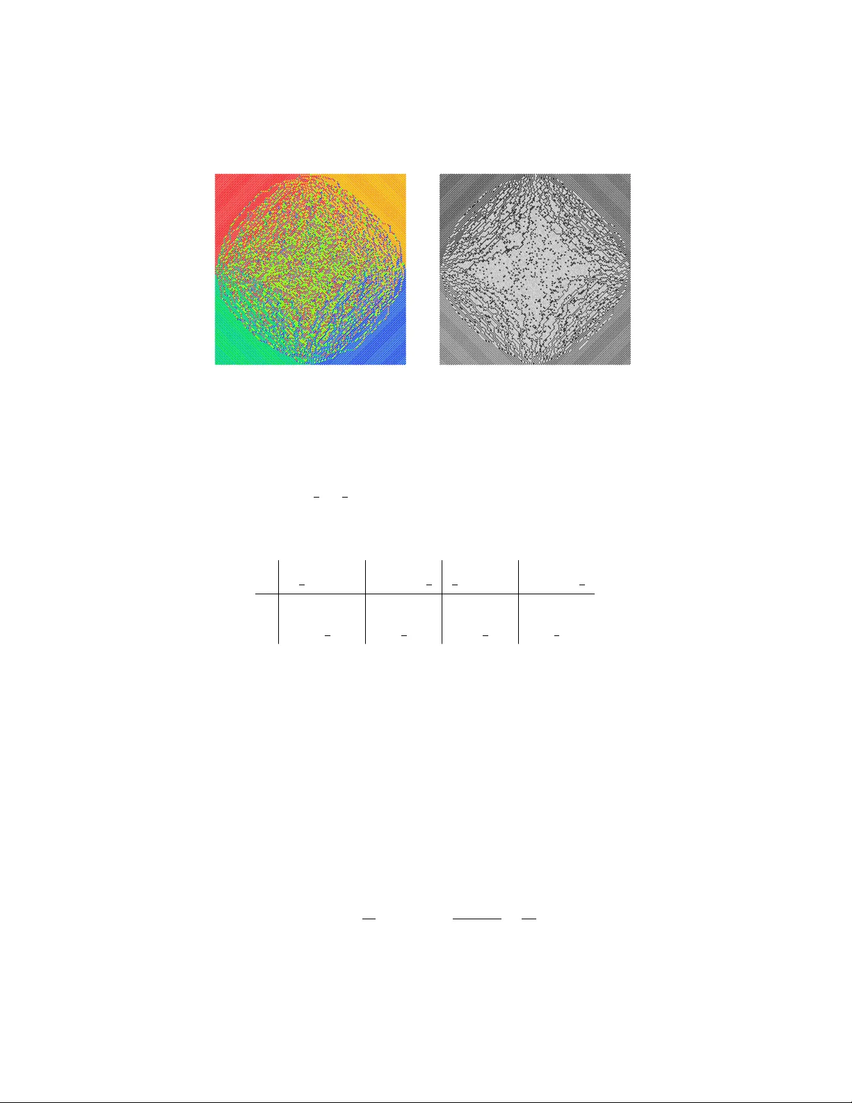
Limit shap es and harmonic tric ks Nik olai Kuc humo v ∗ Marc h 24, 2026 Abstract This article has tw o main goals. First, it provides a self-con tained exp osition of the tangen t plane metho d for the dimer mo del — a tec hnique for analyzing arctic curv es and limit shap es introduced by R. Keny on and I. Prause (2020). Second, it extends this method to multiply connected domains through a nontrivial computation of the frozen b oundary for the Aztec diamond with a hole. This computation yields the first explicit parametrization in terms of elliptic functions of a family of arctic curv es of a m ultiply-connected region indexed b y the height change (hole height). W e also deriv e and visualize the corresp onding limit heigh t functions. 1 In tro duction The planar dimer model has b een an activ e area of researc h for sev eral decades. It originated in the 1960s in the physics literature on equilibrium statis- tical mechanics, in the w orks of Kasteleyn and T emp erley–Fisher [Kas61, TF61]. The mo del later attracted the attention of the mathematical comm unity through studies of the Aztec diamond and its connection to alternating sign matri- ces [Jam03]. This naturally led to the question: What do es a typical domino tiling of a large planar domain lo ok like? The answ er for the large Aztec dia- mond w as given by the Arctic Circle Theorem [JPS98]. Subsequent w ork ex- tended this result to other simply connected regions [CKP00] and to v arious in tegrable domains generalizing the Aztec diamond [BK16, CS16, FL17]. The first analysis of a m ultiply connected region appeared in [BG19], and the cor- resp onding v ariational principle was extended in our previous work [Kuc21]. In the present pap er, we p erform the first explicit computation of a one-parameter family of limit shap es, together with the arctic curves of a multiply connected v ersion of the Aztec diamond parametrized by a mo dular parameter τ . This region is a large Aztec diamond order N with a hole in the center consisting of a smaller Aztec diamond of order ⌊ κ ( τ ) N ⌋ . F or each τ w e compute the asyp- totics of a typical configuration of domino tilings of domain with the hole size κ ( τ ) . Equiv alen tly , one could numerically reverse the dependence and view κ ∗ ˚ Ab o Ak ademi Universit y , nikolai.kuchumov@abo.fi 1 Figure 1: Computer sim ulation of a random domino tiling of Aztec diamond of order AD 500 with a centered hole consising of AD 125 . as the parameter of the family as it is the only "real" physical parameter of the domain. The dimer mo del de als with a finite bipartite graph Γ , and a dimer c onfig- ur ation (or dimer c over ) on Γ is a subset of its edges suc h that eac h vertex is inciden t to exactly one edge in the subset. When Γ is a subgraph of the square grid, dimer cov ers are in bijection with domino tilings of the dual graph of Γ . Abusing notation, we will work with this graph instead. W e think of it as a union of unit squares of the square grid. Let us also fix a c hessb oard coloring, so that we hav e black and white squares (they co exist). Then, let us fix a uniform distribution on the set of domino tilings of Γ . T urns out that the typical domino tiling of a large region exhibit a phenomenon similar to the Aztec diamond. The Aztec Circle Theorem states that a random domino tiling of a large Aztec diamond is fixed outside the inscrib ed unit circle to the rescaled domain, while it remains random inside it. The inner region is the r ough r e gion (liquid region), the asymptotically deterministic regions are fr ozen r e gions , and the curve separating them is the ar ctic curve (frozen curve), whic h is a unit circle for the Aztec diamond, see 2 for a computer simulation. In other regions the same phenomenon(separation of domain into rough and frozen regions) typically o ccurs. A common tool to address this question is to enco de a domino tiling b y the height function . It is a function H D : V (Γ) → Z defined b y a certain com binatorial rule. It turns out that in the limit of a large region, the re-scaled heigh t function appro ximates a contin uous Lipschitz function h with ov erwhelm- ing probability . Moreo ver, in the frozen regions this function is linear with the maximal allow ed slope, while in the rough region its gradient lies strictly inside the Newton p olygon. The main result of [CKP00], the v ariational principle for random domino tilings, c haracterize h as a minimizer of a certain v ariational 2 Figure 2: Uniformly random domino tiling of an Aztec diamond of order 30. function of the form R Ω σ ( ∇ h ) dxdy . Here σ : N → R is a conv ex function called surfac e tension , and N is an integer p olygon, the so-called Newton p olygon of the mo del [KOS06], whic h is the set of allow ed slop es ∇ h ∈ N . The generality of the v ariational approac h is offset by the difficulty of its implemen tation: the singular b eha vior of σ complicates the asso ciated Eu- ler–Lagrange equation. The next step of understanding of this this equation w as done in [KO05], where the authors low ered the order of the Euler–Lagrange equation for lozenge tiling mo del by in tro ducing the so-called c omplex gr adi- ent (complex slop e) map z . It satisfies the complex Burgers equation and the sp ectral curv e condition in the liquid region, where it also defines a non-trivial complex structure. When it is approac hing ∂ L , it gets a singularity . In the in- terior of L , expressed in complex-gradien t coordinates, the Keny on–Okounk ov conjecture predicts that the fluctuations are gov erned by the the pullback of the Gaussian free field from the u pper-half plane H [KO05]. The authors also give an argument of existance of an algebraic arctic curv e for a family of regions in the lozenge tiling mo del using methods of tropic geometry . The mathematically regorous work on existance and algebraic arctic curve for the dimer mo del was done in [ADPZ26]. On the other hand, researchers ha ve found w ays to compute the limit shap e using v arious methods, such as the Sc hur pro cess in tro duced in [OR01] and further developed through representation-theoretic approaches in [BF08, BG19]. More recen t dev elopments include the tangen t metho d, whic h also applies for the six-v ertex mo del [CS16, FG18]. Then, the work [KP22] fo cuses on a systematic approach to the study of limit shap es from the v ariational p ersp ectiv e. It realizes the graph of h ⋆ as the en velope of its tangen t planes P x 0 ,y 0 = { ( x, y , z ) ∈ R 3 | s ( x 0 , y 0 ) x + t ( x 0 , y 0 ) y + c ( x 0 , y 0 ) = z } , 3 supplemen ted by an appropriate tangency condition. The authors parametrize points ( x, y ) ∈ L by a single complex v ariable, the so-called intrinsic co ordinate u = u ( x, y ) , whic h is a ramified co ver of the complex slop e z . This intrinsic co ordinate uniformizes the liquid region Σ → L . Then, by Theorem 1 in [KO05] for random lozenge tilings and Thorem 4.8 [ADPZ26] for the generic p eriodic dimer mo del, the gradient co ordinates s and t are harmonic as functions of u . Moreo ver, the intercept function c is also harmonic by Theorem 3.1 [KP22]. Then, the frozen boundary ∂ L can b e obtained parametrically from ∂ Σ via the tangency condition. One first constructs the harmonic extensions of s ( u ) , t ( u ) , and c ( u ) . The n, for each u ∈ ∂ Σ , one solves the complex tangency equation. s u ( u ) x + t u ( u ) y + c u ( u ) = 0 for the real ( x, y ) . As this is a single complex equation, it imposes tw o real con- strain ts and determines x ( u ) and y ( u ) . The solution ( x ( u ) , y ( u )) parametrizes the frozen b oundary for u ∈ ∂ Σ . F or internal p oin ts u ∈ Σ \ ∂ Σ we obtain ( x ( u ) , y ( u )) ∈ L (Ω) in the liquid region, and the height function as a function of u , h ( u ) = s ( u ) x ( u ) + t ( u ) y ( u ) + c ( u ) , the limit shape can b e computed and plotted numerically . Note ho wev er, that in order say rigorously that suc h h is indeed the solution of the v ariational problem, one would hav e to chec k the frozen star ray prop ert y from Theorem 9.3 [ADPZ26], whic h we omit in this pap er. In the work [KP22] the authors demonstrate harmonicity from the so-called trivial potential property of the dimer model. W e do it in a slightly differen t w ay , and in Proposition 3 and Theorem 1 w e show it directly from the Harnac k prop ert y of the asso ciated sp ectral curv e. Thus, our pro of is v alid as long as the assosiated sp ectral curve is a Harnack curve, for instance for p erio dic weigh ts. It pro vides a clear connection with the work [BB23] later extended to generic sp ectral curv es in [BA24]. The connection is that while we op erate with zeros of a differen tial dF = xds + y dt + dc , in [BB23] the roles of s and t are exchanged compared with our notations. In work [BA24] the corresp onding ob jects are xds = dζ 1 , y dt = dζ 2 and dc = dζ 3 . These t wo articles deal with so-called gaze bubbles, whic h mak e a liquid region m ultiply-connected. How ev er, the underlying domain is still simply-connected unlike our situation. In the present article, we extend the tangent plane metho d to a m ultiply connected domain and compute the family of arctic curves for the Azte c dia- mond with a hole . While the v ariational principle for this case was extended in our previous result [Kuc21], here we provide a concrete example of a family of m ultiply-connected limit shap es. The T angent plane metho d giv es a solution to the v ariational principle, and it op erates directly with contin uous ob jects. Therefore, we do not need to compute discrete data and then pass to the limit that quite often requires the most technical effort, for instance, in the tangent metho d [CS16, FG18]. The tradeoff of this adv antege is that we need to match the critical p oints of s u ( u ) , t u ( u ) and c u inside L , whic h tak es a big effort. One could produce plots of arctic curves without it, how ev er, these curves would be 4 Figure 3: Plot of h for the Aztec dia- mond with a hole - 1.0 - 0.5 0.5 1.0 - 1.0 - 0.5 0.5 1.0  0.120047, 1 4 , 0. + 0.480978  , 0, - 0.869638 + 0.   Figure 4: Arctic curv e of the Aztec diamond with a hole. The y ellow curv e is the outer connected comp o- nen t, while the blue is the inner one. The corresp onding v alues of param- eters a, κ , τ , δ are written abov e the plot. "fak e" as they would not corresp ond to any 3 d surface minimizing the functional. Note that the difficult y of critical p oints emerges only for multiply-connected Ω , and w e do not see it in gas bubbles(there are no suc h critical points), where L is also multiply-connected. W e sho w that in the limit, both the limit shape h , and κ are expressed in terms of elliptic functions. In particular, w e provide a numeric scheme of the computation in which w orks also for the limit shap e of lozenge tilings of a hexagon with a hexagonal hole, which will b e in the next F or instance, κ is giv en by the v alue of an elliptic function ev aluated at a particular p oin t, see (58). F urthermore, a simple brownian motion argument shows that as τ → ∞ harmonic extensions s, t, c conv erge to the ones of usual Aztec diamond with cylindrical parametrization. 1.1 Structure of the pap er The structure of the pap er is the following, • In Section 2 we giv e a review of the complex gradient map in Theorem 1 and then pro ceed to the conformal coordinates in Prop osition 1. Then, w e sho w the harmonicity of the functions s , t , and c in Prop osition 3. W e conclude with the tangen t equation 4 which will b e used to reconstract the arctic curve. 5 • In Section 3 we discuss applications to the domino tilings. In subsection 3.1.2 we discuss limit shape of the Aztec diamond, and then in subsection 3.2 w e discuss Aztec diamond with doubly-p eriodic weigh ts with nessasary bac kground on elliptic functions in 3.2.1. After it, we discuss the main example, Aztec diamond with a hole in subsection 3.3. • App endix A is dev oted to deriv ation of the Beltrami equation in the needed forms. 1.2 A ckno wledgements W e w ould like to thank C´ edric Boutilier for his help throughout this work and for carefully reading the manuscript. This w ork w as supp orted by the Re searc h Council of Finland (gran t 365297). Moreov er, we thank Rick Ken yon and Istv´ an Prause for providing Mathematica co de for the doubly p erio dic Aztec diamond, whic h w as crucial for the w ork. F urthermore, w e thank T omas Berggren for the discussions that led to our numerical sc heme. 2 Assumptions and geometry of the tangent plane metho d W e assume the n umber of frozen regions around eac h connected b oundary comp onen t, and the top ological type of the liquid region. Then, w e write a table consisting of columns with boundary planes at each frozen region. After that w e perform harmonic extensions for s, t and c depending on parameters to b e fixed later. Then, we analize the critical points of deriv atives s u , t u and c u , and in order to matc h them w e fix the parameters, this is the difficult part, whic h is partially a v ailible only n umerically . After that, we are able to pro duce the figure of the Arctic curve, and the graph of h . Also, we are using the Newton polygon for the square lattice turned b y 45 degrees so that the characteristic p olynomial is P ( z , w ) = 1 + z + w − z w and the Newton p olygon is the unit square with vertices (0 , 0) , (1 , 0) , (0 , 1) , (1 , 1) . W e ha ve the follo wing picture going from the boundary of the region to the bulk: near the b oundary ∂ Ω , we hav e frozen, where h is linear with the maximal p ossible slop e, h ∈ ∂ N . The b oundary of this part is the arctic curve C , whic h is smo oth except at finitely man y p oin ts. After crossing the boundary , w e end up in the liquid region, where ∇ h ∈ ˚ N . There, we might hav e another connected comp onen t of the arctic curv e C , which b ounds a gas phase where the gradien t is constant ∇ h = q . Now, we know enough prop erties of ∂ L to p erform some computations, and the main to ol are conformal co ordinates, which help to simplify the analysis of the Euler-Lagrange equations for the dimer mo del. The idea is that we start with the liquid region L , and then assuming that h is the minimizer, w e map the liquid region to the Newton p olygon, ( x, y ) 7→ ( s, t ) := ∇ h ( x, y ) ∈ N . Moreov er, in the pap er [KP22], the authors lo ok at N 6 z w z w 1 π t π s Figure 5: Relation b et ween coordinates ( s, t ) and ( z , w ) as a Riemann surface with the metric g given by the Hessian of surface tension σ : g = σ ss ds 2 + 2 σ st dsdt + σ tt dt 2 . (1) Con vexit y of σ implies that the Hessian is p ositiv e definite, and thus corresp onds to a (non-degenerate) metric. Then, they p erform the main tric k of the method, that is a sp ecific c hange of co ordinates, ( s, t ) 7→ z , for complex v ariables z on the sp ectral curve P ( z , w ) = 0 . The relation betw een ( s, t ) and ( z , w ) can be formulated graphically as on Figure 5. W e justify this figure in Theorem 1 b elo w. In a simple example lik e Aztec diamond, one could use suc h z as a conformal co ordinate and parametrize points of ∂ L by it. In other words, we can enco de p oin ts of ∈ L b y the positive half of the sp ectral curve C + ≃ H . Ho w ever, in a more compicated situatuion, where degree of ∇ h is higher than 1 , for instance in a m ultiply-connected domain, one w ould need to use a ramified co ver of z , Σ → C . Then, the conformal mo del of L is not H , but an ann ulus Σ + ≃ [0 , 2] × [0 , τ ] / ∼ where w e iden tify u and u + 2 . There z b ecomes a meromorphic function of u ∈ Σ , and s, t with c are harmonic maps of this u (as the first tw o are harmonic in terms of z , and harmonicity of c follows from the Harnac k prop ert y of the spectral curv e). The follo wing comm utative diagram illustrates this: L N A Σ + C + Σ C 1:1 ∇ h 1:1 ∇ σ ⊂ deg d (log | z | , log | w | ) ⊂ π There is also a creterion for an instrinsic co ordinate from [KP22], that w e sho w for completness in Prop osition 1. W e begin our pro of of the diagram by sho wing Theorem 1, whic h explains the relation b et ween C + and L . 7 Theorem 1. In the liquid r e gion L , ther e ar e define d two functions z ( x, y ) , w ( x, y ) satisfying the fol lowing pr op erties, 1. ∇ h = 1 π (arg w , − arg z ) , 2. A mp` er e’s e quation z x z + w y w = 0 , 3. sp e ctr al curve e quation P ( z , w ) = 0 . Pr o of. W e start with a point ( z 0 , w 0 ) on the sp ectral curve { P ( z , w ) = 0 } . Then, w e know that the real part of its image under the logarithm map (log | z 0 | , log | w 0 | ) defines a p oin t in the amo eba ( X, Y ) := (log | z 0 | , log | w 0 | ) ∈ A , see also [KOS06][3.2.3]. Here, we assume that ( z 0 , w 0 ) is a generic p oin t, so that ( X, Y ) = (log | z 0 | , log | w 0 | ) is in the interior of A . W e further assume that z 0 ∈ H (so that w 0 has a negative imaginary part). In fact, we kno w from the Harnack property of the sp ectral curv e that there is exactly another ro ot of P , whic h is sen t to the same p oint of the amo eba, giv en by ( ¯ z 0 , ¯ w 0 ) . W e write z 0 = e X + iθ 0 , w 0 = e Y + iω 0 , with θ 0 ∈ (0 , π ) and ω 0 ∈ ( π , 2 π ) . The gradien t of the Ronkin function R ev aluated at this p oin t defines the corresp onding slope ( s, t ) . More precisely , we ha ve the follo wing equation, ( s, t ) := ∇R (log | z | , log | w | ) . (2) Let us compute the deriv ativ es of the R b y definition, s = ∂ ∂ X 1 (2 π i ) 2 Z Z T 2 log P ( e X z , e Y w ) dz dw z w = 1 (2 π i ) 2 Z | w | = e Y Z | z | = e X ∂ X P ( e X z , e Y w ) P ( e X z , e Y w ) dz dw z w ! = 1 2 π i Z | w | = e Y dw w 1 2 π i Z | z | = e X d log P ! , (3) where w e lo ok at  1 2 π i R | z | = e X d log P  as a function of w , which is fixed, and then integrate it o ver the circle {| w | = e Y } . F or a given v alue of w , there is a unique v alue of z = z ( w ) = w +1 w − 1 suc h that P ( z ( w ) , w ) = 0 . It turns out that when w mov es coun terclo c kwise around the circle of radius e Y , the ro ot z ( w ) is inside the disc of radius e X when w is on the arc from ¯ w 0 to w 0 , and outside when w is on the arc from w 0 to ¯ w 0 . As a consequence, the function w 7→ R | z | = e X d log P ( · , w ) is a the indicator function of the arc ( ¯ w 0 , w 0 ) . Therefore, the remaining integral is s = Z w 0 ¯ w 0 1 2 π i dw w = 1 2 π i (log w 0 − log ¯ w 0 ) = 1 2 iπ (log( e Y + iω 0 ) − log( e Y + i (2 π − ω 0 ) )) = ω 0 π − 1 . 8 - 4 - 2 2 4 - 4 - 2 2 4 Figure 6: Plot of Amoeba for Z 2 and our c hoice of P ( z , w ) . Quadran ts corre- sp ond to the frozen regions. The computation for the other co ordinate of the gradient corresp onding to t is the same except that the integral 1 2 iπ R | w | = e Y d log P ( z , · ) is the indicator function of the orien ted arc from z 0 to ¯ z 0 . This means that when we integrate the result ov er z , w e get t = Z ¯ z 0 z 0 1 2 π i dz z = 1 2 π i (log ¯ z 0 − log z 0 ) = 1 2 iπ (log( e X + i (2 π − θ 0 ) ) − log( e X + iθ 0 ) )) = 1 − θ 0 π . As a result, we ha v e that log z 0 = X + π i (1 − t ) , log w 0 = Y + π i (1 + s ) . (4) By a global translation of the set of slop es by the vector (1 , − 1) (or by replacing z by − z and w by − w ), we can assume that the following relation holds log z 0 = X − iπ t, log w 0 = Y + iπ s. (5) W e now asso ciate to each p oin t ( x, y ) of the liquid region a pair ( z , w ) , in suc h a w ay that the argumen ts of z ( x, y ) = z 0 and w ( x, y ) = w 0 matc h the (translated) slop es − t and s resp ectiv ely , times π according to (5). No w, we substitute X , Y from (5) to the intrinsic Euler Lagrange equation, whic h can b e rewritten as X x + Y y = 0 and see that it b ecomes Re( z x z + w y w ) = 0 . This is one real equation, which should be supplemented with a consis- tency condition ∂ s ∂ y = ∂ t ∂ x = ∂ 2 h ∂ y∂ x or − ∂ s ∂ y + ∂ t ∂ x = 0 , which by (2) can be written as ⟨ ( − ∂ ∂ y , ∂ ∂ x ) , ∇R (log | z | , log | w | ) ⟩ = 0 , since ∇R (log | z | , log | w | ) = 1 π (+ arg w, − arg z ) . Th us, we end up with the second real equation Im( z x z + w y w ) = 0 . It completes the deriv ation of the Amp` ere’s equation. 9 It turns out that the co ordinate z itself defines conformal co ordinates ( U, V ) := (Re z , Im z ) . In fact, let us lo ok at (5). Since logarithm is a holomorphic map, it satisfies the Cauch y-Riemann equations, and so does the righ t-hand side. F or example, for Y + iπ s we ha ve tw o equations, Y U = π s V , Y V = − π s U . (6) and for X − iπ t . X U = − π t V , X V = π t U . (7) These equations are combined into complex equations with the help of Wirtinger deriv ativ es, X z = 1 2 ( X U − iX V ) = 1 2 ( − iπ ( s U − is V )) = − iπ s z , Y z = iπ t z . (8) W e also see that Y z s z = iπ = − X z t z , therefore, w e ha ve X z t z + Y z s z = 0 . It is the first criterion for z b eing an intrinsic v ariable from prop osition 2.1 from [KP24]. Then, recall that X = σ s ( s, t ) , Y = σ t ( s, t ) , which enables us writing π s V = Y U = σ st s U + σ tt t U , π t V = − X U = − σ ss s U − σ st t U . (9) This is nothing but the real Beltrami equation, a sufficient condition for the co ordinates ( U, V ) to b e conformal/conformal. Thus, z = U + iV is the in trinsic co ordinate according to the definition of [KP22]. The authors there prop ose a criterion for a co ordinate ζ to b e an in trinsic one, that w e form ulate in the follo wing Prop osition: Prop osition 1 ( [KP22], Proposition 2.1) . The fol lowing two e quations ar e e ach e quivalent to ζ b eing an intrinsic c o or dinate X ζ s ζ + Y ζ t ζ = 0 (10) s ζ t ζ = − σ st − i √ det H σ σ ss (11) A nd in the c ase the ab ove e quations hold, we have X ζ t ζ = − i det H σ = − Y ζ s ζ . (12) Note also that the last relation from Proposition 1 together with (8) implies that det H σ = π 2 . 10 Pr o of. Let us define γ := s ζ t ζ . Then, due to X ζ = ( σ s ) ζ = σ ss s ζ + σ st t ζ , w e write X ζ t ζ = σ ss γ + σ st . Rewriting this computation for Y , we see Y ζ s ζ = σ tt 1 γ + σ st . Therefore, the first condition of Prop osition 10 is nothing but σ ss γ 2 + 2 σ st γ + σ tt = 0 . (13) The tw o roots are γ = − σ st ± i √ det H σ σ ss σ ss . (14) Since in our conv en tion, ζ is assumed to b e orien tation-reversing map, Im( γ ) < 0 and we hav e the minus sign. F urthermore, X ζ t ζ = − i √ det H σ = Y ζ s ζ . No w, with the help of Prop osition 1 w e can prov e the intrinsic Euler-Lagrange equation in tw o forms, Prop osition 2. F or ( x, y ) ∈ L we have X ζ ζ x + Y ζ ζ y = 0 , (15) ζ x ζ y = s ζ t ζ = γ . (16) Pr o of. The last expression of the pro of of Prop osition 1 implies that (we are using the chain rule for X x = X ζ ζ x + X ¯ ζ ¯ ζ x and ¯ f ( ¯ z ) = ¯ f ( z )) , X x − i p det H σ t x = X ζ ζ x + X ¯ ζ ¯ ζ x − i p det H σ ( t ζ ζ x + t ¯ ζ ¯ ζ x ) = (17) = ( X ζ − i p det H σ t ζ ) ζ x + ( X ζ + i p det H σ t ζ ) ζ x = 2 X ζ ζ x . (18) Similarly for Y , Y y + i p det H σ s y = 2 Y ζ ζ y . (19) Therefore, since t x = s y w e hav e the following intr insic Euler-Lagrange equation X ζ ζ x + Y ζ ζ y = 0 . (20) Let us look at (5), the left-hand side X − iπ t is a holomorphic function of ζ , as well as Y + iπ s . Therefore, they satisfy the Cauch y-Riemann equation, whic h tells us that X ζ = iπ t ζ , (21) Y ζ = − iπ s ζ . (22) Whic h in combination with X ζ ζ x + Y ζ ζ y = 0 giv es us that t ζ ζ x − s ζ ζ y = 0 or t ζ s ζ = ζ y ζ x = 1 γ . Then, apply the Prop osition 2 com bined with the relation − y ¯ z x ¯ z = z x z y . It follo ws from z = z ( x, y ) , where w e take the deriv ativ e with resp ect to ¯ z and obtain 0 = z x x ¯ z + z y y ¯ z . Finally , we get − y ¯ z x ¯ z = z x z y = s z t z , and we are done. 11 Ho wev er, one can see that z is a conformal coordinate directly from the equa- tion we already ha ve. Let us show that the metric g in coordinates ( U, V ) is di- agonal, i.e., that the scalar pro duct g ( ∂ ∂ U , ∂ ∂ V ) = 0 and g ( ∂ ∂ U , ∂ ∂ U ) = g ( ∂ ∂ V , ∂ ∂ V ) . F or this, let us note the expressions for the vector fields in co ordinates ( s, t ) . ∂ ∂ U = s U ∂ ∂ s + t U ∂ ∂ t , ∂ ∂ V = s V ∂ ∂ s + t V ∂ ∂ t . No w, the scalar pro duct g ( ∂ ∂ U , ∂ ∂ V ) equals to σ ss s U s V + σ st ( s V t U + s U t V ) + σ tt t U t V . (23) Then, using (5) we ha ve π s V = Y U = σ st s U + σ tt t U , π t V = − X U = − σ ss s U − σ st t U . (24) It helps us to express the deriv atives with resp ect to V through deriv atives with resp ect to U in (23), let us write each term of (23) and mark by the same color the terms which cancel eac h other in the sum (23). π σ st t U s V = σ 2 st s U t U + σ st σ tt t 2 U , π σ st s U t V = − σ ss σ sts 2 U − σ 2 st s U t U π σ ss s U s V = σ ss σ st s 2 U + σ ss σ tt t U s U π σ tt t U t V = − σ ss σ tt t U s U − σ st σ tt t 2 U As for the diagonal elements of the metric, w e hav e g ( ∂ ∂ U , ∂ ∂ U ) = σ ss s 2 U + 2 s U t U σ st + σ tt t 2 U , (25) g ( ∂ ∂ V , ∂ ∂ V ) = σ ss s 2 V + 2 s V t V σ st + σ tt t 2 V . (26) Let us rep eat the same steps and express deriv ativ es with resp ect to V , (note that w e ha ve an extra multiple π in (24), which app ear eac h time we transform deriv ative with resp ect to V into deriv ative with respect to U ) 1 π 2 ( σ ss ( σ st s U + σ tt t U ) 2 + 2 σ st ( σ st s U + σ tt t U )( − σ ss s U − σ st t U ) + σ tt ( σ ss s U + σ st t U ) 2 ) . (27) Then, comparison of co efficien ts in front of s 2 U sho ws that in (25) we ha ve σ ss , while in (27) we ha v e 1 π 2 σ ss ( σ 2 st − 2 σ 2 st + σ tt σ ss ) = σ ss σ ss σ tt − σ 2 st π 2 = σ ss (28) 12 (terms whic h con tribute to the coefficient are in the oliv e color). A similar computation done for co efficien ts in front of t 2 U sho ws that (the terms are in the red color), on one hand, we get σ tt , while on the other hand 1 π 2 σ tt ( σ ss σ tt − σ 2 st ) = σ tt . (29) Finally , the same computation sho ws agreement for the co efficien t in front of s U t U , 2 σ s,t on one hand, and 1 π 2 (2 σ s,t ( σ s,s σ t,t − σ 2 s,t − σ t,t σ s,s + σ t,t σ s,s )) = 2 σ s,t on the other. 2.1 An in termediate parameterization It may happ en that there are several p oin ts in the liquid region with the same slope ( s, t ) ∈ ˚ N \ G . In that case it is not possible to parameterize the liquid region by the slop e, and th us by the coordinate z . Ho wev er, the degree d of ∇ h : L → ˚ N \ G is constan t except man y at a finite num b er of p oin ts. W e can therefore introduce a ramified co vering Σ of degree d ov er the sp ectral curv e { P ( z , w ) = 0 } suc h that the v ariables z and w are now meromorphic functions of the v ariable u ∈ Σ . Let Σ + the preimage b y z of the upp er-half plane. This giv es a diffeomorphism from Σ + to the liquid region. The functions s and t , considered b efore as functions of z , can b e now seen also as functions of u ∈ Σ + . 2.2 The in tercept function Let us lo ok at the graph of the minimizer h ⋆ . More precisely , tak e the tangen t plane P x 0 ,y 0 to it at a giv en point ( x 0 , y 0 ) . It has a slope giv en b y ∇ h ⋆ ( x 0 , y 0 ) = ( s ( x 0 , y 0 ) , t ( x 0 , y 0 )) . It also in tersects the v ertical axis at the ordinate ( h ⋆ − ( sx + ty )) . The function c := h ⋆ − sx − ty is called the inter c ept . With its help, w e can parametrize the tangen t planes to the plot of h ⋆ as follows, P x 0 ,y 0 = { ( x, y , z ) ∈ R 3 |{ s ( x 0 , y 0 ) x + t ( x 0 , y 0 ) y + c ( x 0 , y 0 ) = z } . (30) The imp ortan t prop erties of c for us are first, it is constant on every frozen region since on eac h frozen region h ⋆ is linear with a fixed slope, and so is its tangent plane. Th us, after subtracting the linear part of h ⋆ , the difference tak es a constan t v alue on each frozen region. F urther, the minimizer h ⋆ can b e reconstructed from s , t and c as h ⋆ = sx + ty + c . After it, the limit shap e is obtained as the en velope of planes giv en b y (30). The main property of these planes is harmonicity of functions s , t and c as functions of the conformal co ordinate, whic h is discussed in the next section. 2.3 Harmonicit y of s, t and c The prop ert y of functions s, t and c as functions of conformal co ordinate u is that they are harmonic by Theorem 3.1 from [KP22]. 13 No w, let us re-formulate Prop osition 1 in real terms and prov e harmonicity of s, t and c in conformal co ordinates. Prop osition 3. The functions s , t and c ar e harmonic in the variable u ∈ Σ + . Pr o of. F unctions s and t are harmonic in the v ariable u since they are equal to the argument (imaginary part of the logarithm) of z and w , which are holomor- phic functions of u in the interior of Σ + . Next, consider c = ( h − ( sx + ty )) , and let us apply to it ∂ u and ∂ ¯ u remem- b ering that ∇ h = ( h x , h y ) = ( s, t ) , c u = ( h − ( sx + ty )) u = h x x u + h y y u − ( s u x + t u y + sx u + ty u ) = − s u x − t u y . (31) Then, applying ∂ ¯ u w e obtain by harmonicit y of s, t ∂ ¯ u ( s u x + t u y ) = s u x ¯ u + t u y ¯ u . (32) Moreo ver, taking the deriv ative of u = u ( x, y ) with respect to ¯ u (whic h giv es 0), we get b y the c hain rule: 0 = u x x ¯ u + u y y ¯ u . Since u is lo cally a holomorphic function of z , it is also an intrinsic co ordinate. W e can therefore apply Prop osition 2, and get − y ¯ u x ¯ u = u x u y = s u t u , from which it follows that ∆ u c = 4 c u, ¯ u = 0 . Therefore, we can hop e to reconstruct all three functions as long as we are able to p erform explicit harmonic extensions of piecewise constan t b oundary conditions. As a corollary , w e can obtain the limit shape h ⋆ as en velope of harmonically mov ing planes b y Theorem (2), see also [KP22, Theorem 3.2], 2.4 T angen t plane equation In tro duce the main equation of the metho d, Equation (20) from [KP22], whic h will help us to compute the arctic curve. Prop osition 4. Inside the liquid r e gion, p ar ameterize d by u ∈ Σ + , the fol lowing e quation holds: s u x + t u y + c u = 0 (33) What is imp ortan t is that this complex equation is equiv alent to t w o real equations for the real and imaginary parts, whic h gives for ev ery u ∈ Σ + a linear system for ( x ( u ) , y ( u )) , once w e know s , t , and c as functions of u . 14 Pr o of. Let us apply the Wirtinger deriv ative ∂ u to the minimizer h , remembering that ∇ h = ( s, t ) , we ha ve the follo wing equalities h u = sx u + ty u = ( sx + ty ) u − ( s u x + t u y ) (34) s u x + t u y + ( h − ( sx + ty )) u = 0 , (35) whic h is the same as s u x + t u y + c u = 0 . (36) In practice, we deal with harmonic extensions made of linear combinations of arg( u ) , the important identities are first arg( u ) = Im log( u ) , which we use to tak e the Wirtinger deriv ative as ∂ u arg( u ) = 1 2 i 1 u . (37) As a corollary of (3) and (4), we obtain the plot of the minimizer h ⋆ o ver Σ + can b e recov ered as an env elop e of harmonically moving planes with the slop e giv en by ( s ( u ) , t ( u )) , u ∈ Σ + . Theorem 2 (Theorem 3.2 [KP22]) . The gr aph of the minimizer h ⋆ over u ∈ Σ + is the envelop e of harmonic al ly moving planes P u that satisfy two c onditions: • P u := { ( x ( u ) , y ( u ) , z ( u )) ∈ R 3 | xs ( u ) + y t ( u ) + c ( u ) = z ( u ) } • s u x + t u y + c u = 0 Her e, x and y ar e functions of u . 3 Applications for the random domino tilings In the rest of the chapter, we are going to explain the metho d applied to a simply-connected domain, the Aztec diamond, and to our main example, the Aztec diamond with a hole. W e also need to use assumptions for the num b er of frozen regions of the particular domains, and v alues of s, t and c there. This data is inferred from discrete b oundary conditions and computer simulations. F or the square grid, w e can tak e the fundamental domain represented on Figure 7, the corresp onding Kasteleyn op erator is giv en by K ( z , w ) = 1 + z + w − z w. (38) 15 Figure 7: W eigh ts of the fundamen tal domain of the square grid with A y and B x cycles. The reference dimer cov er is in dashed color. Figure 8: Example of the Aztec diamond of order 4 on the left, and a domino tiling of it on the righ t, with four types of domino es according to the c hess-b oard coloring. 3.1 A case with a simply-connected liquid region: the uni- form Aztec diamond Recall that the Aztec diamond of order N is the union of unit squares S ( m, n ) of the square lattice whose centers ( m, n ) satisfy | m − 1 2 | + | n − 1 2 | ≤ N . (39) It is also conv enient to in tro duce chess-board coloring on the square grid, this w ay w e obtain 4 types of domino es, see Figure 9. W e consider in this section the case of the uniform measure on tilings of the Aztec diamond of size N . As N goes to infinity , a random height function con verges in probability to a deterministic function which is linear in the four regions in the limiting renormalized square depriv ed of the inscrib ed disc (the fr ozen r e gions ) and is smo oth inside the inscrib ed disc (the liquid region). This statemen t is due to Jo c kush, Propp and Shore [JPS98]. The goal of this section is to reco ver this result using the tangen t plane method, describ ed ab ov e, following lo osely [KP22, Section 6.1],[Section 2.3] [KP24]. 3.1.1 Applying the tangen t plane metho d In the case of the uniform Aztec diamond, it is conv enient to use a co ordi- nate system ( x, y ) in the renormalized domain wic h is rotated b y 45 degrees with 16 Figure 9: Example of the same domino tiling in color notation, and domino tiling of Aztec diamond of order 50 by J.Propp. resp ect to the horizon tal/vertical discrete co ordinate axes, so that the renormal- ized domain becomes in the limit the unit square [0 , 1] × [0 , 1] . See Figure 11 to see the directions of the tw o axes for x and y . In the liquid region L , there is a unique point where the limiting heigh t function has a given slop e in the in terior of the Newton p olygon (the fact that eac h of the four frozen phases is seen only once on the b oundary of L is a sign that the degree d from u to z or w is 1). This is thus a case when we can take u = z : the liquid region can b e paramaterized b y z ∈ H . W e no w determine the v alues for s , t and c on the b oundary of the liquid region (whic h corresponds to z ∈ R ∪ {∞} , b ounded by the four distinct frozen regions. Eac h interv al ( −∞ , − 1) , ( − 1 , 0) , (0 , 1) , (1 , ∞ ) corresp onds to an arc of the arctic curve touching a giv en frozen phase, with slope ( s, t ) giv en respectively (with the conv ention of the slop e given b y Equation (4)) b y (1 , 0) , (0 , 0) , (0 , 1) and (1 , 1) respectively . W e form a table consisting of four columns for each frozen region, and three ro ws for each function s , t and c . (1) (2) (3) (4) z < − 1 − 1 < z < 0 0 < z < 1 1 < z 1 > w > 0 0 > w > − 1 − 1 > w w > 1 s 1 0 0 1 t 0 0 1 1 c 0 1 0 0 The v alue of c is determined up to some additive constan t, fixed here to b e zero. Its v alue in eac h region is fixed by the condition that the linear parts of the heigh t functions with the given slop es in the table should match at the “turning p oin ts”, where tw o frozen regions touc h on the b oundary of the Aztec diamond. See Figure 10 for a picture of those linear pieces. W e represen t visually on Figure 11 the information of the table, and four sp ecific v alues of z at the transition b etw een tw o frozen phases near the arctic curv e. 17 Figure 10: Height ab o v e the frozen regions of the Aztec diamond, which is a piecewise linear function. The v alues of c on each arc of the arctic curv e reflect the contin uit y of the height along the b oundary of the liquid region. x y (1) : x (3) : y (2) : 1 (4) : x + y 0 − 1 1 ∞ Figure 11: The four frozen phases of the Aztec diamond, with colors corresp ond- ing to branches of the b oundary of the amo eba from Figure 6. F or each region, w e indicate in blac k the equation for the ordinate as an affine function of x and y . F or each “turning p oin t”, we indicate in purple the corresp onding v alue of z in the parametrization. 18 3.1.2 P arametrization of the limit shap e of the Aztec diamond W e know that s , t and c are harmonic functions of the v ariable z . W e construct explicit harmonic extensions of the b oundary v alues from the table. F or s and t , the answer is given directly by Equation (4), whic h can b e rewritten as s ( z ) = 1 π arg( − w ( z )) = 1 π arg z + 1 z − 1 , t ( z ) = − 1 π arg( − z ) = 1 − 1 π arg( z ) . F or c , w e pro ceed with the same idea, using building blo cks of the form f ( z ) = 1 π arg z − b z − a whic h is the harmonic extension of the indicator function of in terv al [ a, b ] . The corresp onding harmonic extensions is: c ( z ) = 1 π ( − π + arg( z − 1)) . Another choice of conformal co ordinate instead of z which will b e useful in connection with the next example is choosing ζ = 2 π arctan z , whic h maps the complex plane to an infinite cylinder C / 2 Z . The upp er-half plane for z parametrizing the liquid region (resp ectiv ely the real axis together with the p oin t at infinit y parametrizing the arctic curve) is mapp ed to the upper half of the cylinder (resp ectiv ely to R / 2 Z ). The table of b oundary conditions of s, t and c for AD for the v ariable ζ is the follo wing (where the in terv als for ζ represent a cyclic order, as on the cylinder, − 1 = 1 ): (1) (2) (3) (4) − 1 < ζ < − 1 2 − 1 2 < ζ < 0 0 < ζ < 1 2 1 2 < ζ < 1 s 1 0 0 1 t 0 0 1 1 c 0 1 0 0 The harmonic extensions in this parametrization are given by the pullbac k under the map z 7→ 2 π arctan( z ) , that is, b y a comp osition with the map ζ 7→ tan( π ζ 2 ) . s ( ζ ) = 1 π arg 1 − tan( π ζ 2 ) 1 + tan( π ζ 2 ) = 1 π arg tan( π 2 ( 1 2 − ζ )) , t ( ζ ) = 1 − 1 π arg(tan( π ζ 2 )) , c ( ζ ) = 1 π arg tan( π 2 ζ ) tan( π 2 ζ ) + 1 . 19 No w, we need to plug them in to linear system for ( x, y ) given by Equation (4). F or it, we need deriv atives of s, t and c . Recall that we differentiate the arg z b y applying the Wirtinger deriv ativ e using the identit y arg( z ) = Im log z , whic h giv es a factor i 2 to each arg , and therefore factorizes. Thus, we present deriv atives without this common factor. In the coordinate z after a common m ultiplication by 2 π i , w e hav e 2 iπ s z = 1 z − 1 − 1 z + 1 = 2 z 2 − 1 , 2 iπ t z = 1 z , 2 iπ c z = 1 z − 1 z + 1 = 1 z ( z + 1) . With the help of expressions, we can build parametric plots using linear system s z x + t z y + c z = 0 for finding ( x ( z ) , y ( z )) , which contin uously dep ends on z , and then b y inv ersion, compute for ev ery ( x, y ) in the liquid region the v alue of s ( x, y ) , t ( x, y ) , c ( x, y ) , which w ould giv e the equation of the tangen t plane to the limit shape ab o ve the p oin t ( x, y ) . This would finally allow us to reconstruct the limiting height function h as the env eloppe of this family of tangen t planes. But b efore that, there is something simpler we can do: w e can look at the image of ∂ H by the map z 7→ ( x ( z ) , y ( z )) whic h corresp onds exactly to the arctic curve, that is the b oundary of the liquid region. F urthermore, from a computational point of view, it may be hard to give an analytical expression for the solution ( x ( z ) , y ( z )) (except for the uniform Aztec diamond in co ordinate z , as w e will see). Rather, w e can instead for each z compute the linear system and its solution, ( x ( z ) , y ( z )) and plot it by v arying z . In fact, the functions defining the coefficients may not well-defined precisely on the boundary , th us if we try to do it numerically , we add a small p ositive imaginary part to z . This reflects the fact that gradient ∇ h is defined only in the interior of the liquid region, and not on the arctic curve. Re( s z ) x + Re( t z ) y + Re( c z ) = 0 , (40) Im( s z ) x + Im( t z ) y + Im( c z ) = 0 . (41) This is the approach w e will use for the next examples. But it turns out, as it is often the case for the Aztec diamond, that compu- tations are quite easy , and we can find x ( z ) , y ( z ) for ev ery z ∈ H b y solving the simple linear system, x ( z ) = | z − 1 | 2 2( | z | 2 + 1) , y ( z ) = 1 1 + | z | 2 , (42) or ev en in vert it to find z ( x, y ) . Indeed, the tw o real equations (40) and (41) are equiv alen t to the degree-2 complex equation in z : 2 z x + ( z 2 − 1) y − z + 1 = 0 , 20 0.0 0.2 0.4 0.6 0.8 1.0 0.0 0.2 0.4 0.6 0.8 1.0 Figure 12: Left: the argumen t of z ( x, y ) for ( x, y ) in the liquid region. Cy an means that z is pure imaginary , purple and pink (close to the righ t b oundary) corresp ond to z near R − , whereas yello w and orange (on the left) means that z is close to R + . Right: a large piece of the arctic curve obtained from the parametrization b y Equations 42, for z real betw een − 20 , 20 . One can see that the b ottom of the circle is cropp ed, meaning that this part corresp onds to z in a neigb ourhoo d of ∞ . for which we search the solution with p ositiv e (or rather non-negative) ro ot, whic h is given b y: z ( x, y ) = 1 − 2 x + i p 1 − (2 x − 1) 2 − (2 y − 1) 2 2 y , A t this p oin t, w e already recognize the arctic circle of radius 1 2 and center ( 1 2 , 1 2 ) as the limit of definition of the square root defining z : this corresp onds to the b oundary of the liquid region. As mentionned b efore, another wa y to reco ver a parametrization of the arctic curve w ould b e to tak e the solutions from Equation (42) and plot it for z ∈ R ∪ {∞} . See Figure 12 for a plot of the argumen t of z across the liquid region, and for a parametric plot of the arctic curv e. Remark 1. Inste ad of taking the smal lest fundamental domain with one white and one black vertex, and c onsidering the sp e ctr al curve for it, one c ould have taken a fundamental domain made of two white and two black vertic es forming a 2 × 2 -squar e. Se e Figur e 13. The c o or dinate axes ( x, y ) ar e now aligne d with the horizontal and vertic al axes of the squar e lattic e, so that the r enormalize d domain is a r otate d squar e | x | + | y | ≤ 1 . If we lab el with 1 the vertic es on the top r ow, and with 2 those of the se c ond r ow of the fundamental domain, the mo difie d Kasteley matrix K ( z , w ) is given by K ( z , w ) =  1 − w z − 1 1 z − 1 1 w − 1  (43) 21 - - - - w − 1 z − 1 z w (4) (2) (1) (3) Figure 13: Left: a 2 × 2 -fundamen tal domain for the square lattice. Kasteleyn min us signs are indicated on the edges, as well as the extra factors z ± 1 and w ± 1 for edges crossing the fundamental domain. Righ t: the Newton p olygon of the corresp onding c haracteristic p olynomial. and the char acteristic p olynomial c an b e written as − 4 + z + w + 1 z + 1 w . Se e Figur e 13, right for the Newton p olygon of this char acteristic p olynomial, and Figur e 14 for its amo eb a, with the indic ation of the four fr ozen phases. A similar table for b oundary values of s , t and c . (1) (2) (3) (4) s 1 0 − 1 0 t 0 − 1 0 1 c − 1 2 1 2 − 1 2 1 2 Note that in that c ase, z itself do es not p ar ametrize the liquid r e gion: for a given value of z , ther e ar e two values of w such that ( z , w ) is on the sp e ctr al curve. However, one c an p ar ametrize b oth z and and w using r ational fr actions of a variable u living on the Riemann spher e, which c ould b e chosen as the c onformal c o or dinate. 3.2 A case with a m ultiply-connected liquid region, Aztec diamond with t w o-p erio dic weigh ts W e follo w lo osely the discussion here [KP24, Section 2.3]. Before analysis of a m ultiply-connected region, let us discuss our exam- ple with a m ultiply-connected liquid region, where the region is the simply- connected, but the liquid region is non simply-connected due to presence of smo oth or gas phase, so-called bubble. This can be achiev ed for non-uniform distribution on the set of dimer configurations, and the most common example of such phenomenon is the doubly-p erio dic Azte c diamond [CJ14, KP24]. This system of weigh ts for the square lattice is related to the dimer mo del on the square-o ctagon graph: there is a weigh t-preserving corresp ondence b et ween configurations on the tw o lattices (obtained by p erforming the so-called spider move or squar e move ), whic h maps domino tilings of doubly-p erio dic square grid to dimer configurations on the square-o ctagon lattice as long as the weigh ts a 2 = 2 b from Figure 15. 22 - 4 - 2 2 4 - 4 - 2 2 4 (4) (2) (1) (3) Figure 14: Amoeba of the c haracteristic polynomial − 4 + z + w + 1 z + 1 w . The con- nected components of the complement are lab eled with num b ers corresp onding to frozen phases and vertices of the Newton p olygon, together with the corre- sp onding t yp e of edges. a a a a a a a a a a a a a a a a a a a a a a a 1 1 1 1 1 1 1 1 1 1 1 1 1 1 1 1 1 1 1 1 1 1 1 1 1 1 1 1 1 1 1 1 Figure 15: Edge weigh ts of the square grid on the left, and the corresponding w eights of the octagon lattice on the righ t, the corresp ondence b et ween w eights is a 2 = 2 b . 23 - 4 - 2 2 4 - 4 - 2 2 4 Figure 16: Amo eba of the 2-p eriodic weigh t function on the square lattice, for b = 0 . 5 . The hole in the middle corresp onds to the gas or smo oth phase of the corresp onding dimer mo del, which describ es the bubble appearing in the middle of the pictures of Figure 17. In that case, the mo dified Kasteleyn matrix from (43) b ecomes K ( z , w ) =  b − w z − b 1 z − b 1 w − b  (44) and the c haracteristic p olynomial is − 2(1 + b 2 ) + b ( z + w + 1 z + 1 w ) . See Figure 16 for its amo eba. The spectral curve is a genus 1 algebraic curv e C if b  = 1 , which is a Harnac k curv e. It can b e uniformized to a rectangular torus C / (2 Z + 2 τ Z ) , with τ ∈ i R ∗ + : there is a birational m ap ψ : ζ ∈ torus 7→ ( z ( ζ ) , w ( ζ )) ∈ C . See for example [BCdT23, Section 5] and [BdT24, Prop osition 9]. The relation b et w een b and τ (assuming that b < 1 , there is a symmetry b ↔ 1 b ) is given by b = √ k ′ , with k ′ = θ 4 (0 | τ ) 2 θ 3 (0 | τ ) 2 . In particular, for τ = 1 , k ′ = 1 √ 2 , and b = 2 − 1 / 4 . Based, for example, on computer simulations Figure 17 of domino tilings of the doubly-p eriodic Aztec diamond on Figure 17, w e see the presence of all three phases, frozen, rough and smo oth, together with the arctic curve with tw o connected comp onents, the outer curve separating frozen and rough regions, and the inner curve separating rough and smo oth phase regions. This is again a situation where there is a unique point in the liquid region for a given slop e in the Newton polygon. The restriction of ψ to the ann ulus A = R / 2 Z × (0 , Im τ ) parametrizes the upp er half of the spectral curv e C + , and thus ζ ∈ A gives a parametrization of the liquid region. The lo wer b oundary of the ann ulus is mapp ed to the outer b oundary of the liquid region (the liquid/solid 24 Figure 17: Random domino tiling of doubly-p eriodic Aztec diamond for b = 0 . 5 in tw o represen tations, the color representation on the left with e igh t colors to distinguish rough and smo oth phases, and with eight different gra y colors on the right. in terface): up to a horizontal translation, we ma y assume that the turning points corresp ond to ζ = − 1 2 , 0 , 1 2 , 1 (mod 2). The upp er b oundary is mapp ed to the inner b oundary of the liquid region (the liquid/gas interface). The b oundary conditions along the outer b oundary are the same as in the uniform case: (1) (2) (3) (4) − 1 2 < ζ < 0 0 < ζ < 1 2 1 2 < ζ < 1 1 < ζ < 3 2 s 1 0 − 1 0 t 0 − 1 0 1 c − 1 2 1 2 − 1 2 1 2 In order to p erform harmonic extensions in a multiply-connected domain, w e need a particular to olbox of sp ecial functions. Basically , we are going to apply the same strategy: first, write down a basic building blo c k, and then construct harmonic extensions in terms of these building blo c ks. Since the sp ectral curve is a torus, these blocks will be constructed from elliptic functions that we discuss no w. 3.2.1 Elliptic functions and their classification by W eierstrass func- tions Let Λ b e a lattice generated b y tw o vectors ω 1 and ω 2 called p eriods of Λ , Λ := { nω 1 + mω 2 : n, m ∈ Z } . Then, a Λ -elliptic function is a meromorphic function on C that satisfies f ( z ) = f ( z + ω 1 ) = f ( z + ω 2 ) . The most famous example of elliptic functions is W eierstrass’s ℘ -function, whic h is defined as ℘ ( z , Λ) := 1 z 2 + X λ ∈ Λ \{ 0 }  1 ( z − λ ) 2 − 1 λ 2  . (45) 25 The function ℘ clearly has p oles of order tw o at each lattice p oint. It is an elliptic function, which follows from the definition. F or the next subsections, we need tw o other W eierstrass functions. The W eierstrass ζ -function is a function fixed by the equation dζ ( z , Λ) dz = − ℘ ( z , Λ) . (46) This defines it up to an additive constan t that we fix in a w a y that lim z → 0 ζ ( z , Λ) − 1 z = 0 . Using ellipticity of ℘ one can derive quasi-p erio dic prop erties of ζ W eier- strass function, ζ ( z + ω i ) = ζ ( z ) + 2 η i , where η i = ζ ( ω i / 2) . The W eierstrass σ -function is defined b y d log ( σ ( z , Λ) dz = ζ ( z , Λ) . (47) Here, we fix an in tegration constant so that lim z → 0 σ ( z , Λ) − z = 0 . by definition of σ and quasi-p erio dicit y of ζ one derives quasi-perio dicit y of σ , σ ( z + ω i ) = e − 2 η i ( z + ω i / 2) σ ( z ) . (48) F unction σ is a suitable building blo c k of elliptic functions, and every elliptic function can b e expressed in terms of W eierstrass σ function [N.I90]. Theorem 3. Supp ose f is an el liptic function with p erio ds ω 1 , ω 2 and set of zer o es in a fundamental domain of Λ at p oints { κ i } of the c orr esp onding or ders { n i } and set of p oles { κ ′ i } of the or ders { n ′ i } subje ct to two c onditions: • P n i κ i = P n ′ i κ ′ i , • P n i = P n ′ i . A nd let us define a function g as g ( z ) := Q i σ ( z − κ i , Λ) n i Q i σ ( z i − κ ′ i , Λ) n ′ i . (49) Then, the r atio f g is c onstant on C . Pr o of. First, g is elliptic by quasi-p eriodicity of σ recalled in Equation (48), and b y (49). Simply the translation of the function by a perio d ω i do es not change its v alue by our assumptions, g ( z ) 7→ g ( z + ω i ) = g ( z ) exp ( − 2 η i ( P n i κ i − P n ′ i κ ′ i )) = g ( z ) . Moreov er, b y (49) it has the same zero es and p oles with the same mul- tiplicities as f . Thus, the ratio f ( z ) g ( z ) has no zeroes or p oles on C , and thus is constan t by Liouville’s theorem. In our case, Λ = 2 Z + 2 τ Z , so that ω 1 = 2 and ω 2 = 2 τ . Theorem 3 allo ws us to explicitly write the harmonic extensions of piecewise constan t b oundary conditions, whic h we encounter in the tangent plane metho d. Recall the simplest Dirichlet b oundary condition on H , 1 on the negative real 26 line, and 0 on R R ≥ 0 . The harmonic extension is giv en b y 1 π arg z . Now, if w e lo ok at annulus A r 1 ,r 2 = { z ∈ C | r 1 < | z | < r 2 } with b oundary condition of 0 on the outer circle and 1 on the arc connecting ω 0 and ω 1 on the inner circle. The harmonic extension in this situation is 1 π arg z − ω 0 z − ω 1 log | z | r 2 r 1 r 2 . No w, suppose we hav e in terv al ( a, b ) on the upp er side of side of the rectangle [0 , 1] × [0 , | τ | ] . Then, the harmonic extension of b oundary condition 1 on this in terv al and 0 elsewhere is given b y the following form ula h ( u ) = 1 π arg σ ( u − b − τ ) σ ( u − a − τ ) + 2 η 1 (1)( b − a )Im( τ − u ) | τ | . (50) T ake a p oin t u on the upp er b oundary and the complex conjugate u ⋆ . On one hand, f ( u ⋆ ) = f ( u ) as their difference is exactly the p erio d of elliptic func- tion. But on the other hand, since f ( z ) tak es real v alues on R , by the Sc hw arz reflection principle we ha ve f ( ¯ z ) = ( f ( z )) . Th us, the v alues at p oints u, u ⋆ are real since they do not change under complex conjugation( f ( u ) = f ( u ⋆ ) = f ( u ) ). Therefore, the argument from (50) v anishes. W e also need to take deriv atieves of suc h extensions. Let us compute the ∂ u h ( u ) for whic h w e take the branch of argumen t b y arg u = Im log u for the logarithm with branch cut along the real line. First, for z = x + iy w e hav e use the Wiertinger deriv ative to deferen tiate with resp ect to z (as Im z is not a holomorphic function). ∂ ∂ z Im z = 1 2  ∂ ∂ x − i ∂ ∂ y  y = 1 2 i . (51) Then, by the chain rule w e hav e ∂ u h ( u ) = ∂ u  Im log σ ( u − b − τ ) σ ( u − a − τ ) + 2 η 2 ( τ )( b − a ) Im( τ − u ) | τ |  = 1 2 i ( ζ ( u − b − τ ) − ζ ( u − a − τ ) − 2 η 2 ( τ )( b − a )) . (52) 3.2.2 Applying the tangen t plane metho d The solution from [KP24], adapted to our normalization, is the follo wing, s ( ζ ) = 1 π arg σ ( ζ ) σ ( ζ − 1 2 ) σ ( ζ − 1) σ ( ζ + 1 2 ) , t ( ζ ) = 1 π arg σ ( ζ + 1 2 ) σ ( ζ ) σ ( ζ − 1 2 ) σ ( ζ + 1) , , c ( ζ ) = 1 2 + 1 π arg σ ( ζ + 1 2 ) σ ( ζ − 1 2 ) σ ( ζ − 1) σ ( ζ ) − 1 4 Im( ζ ) The functions s and t are argumen ts of gen uine elliptic functions in the v ariable ζ on the whole torus, b y Theorem 3. F or the function c , the zeros 27 - 0.5 0.5 1.0 1.5 - 2 - 1 1 2 Figure 18: Plot of the functions s , t , and c for ζ on (in fact v ery close to) the lo wer b oundary of the cylinder A , matching the table, s in blue, t in yello w and c in green. and the p oles of the fraction in the argumen t are fixed b y the wan ted b eha vior along the outer b oundary , but this do es not define a prop er elliptic function as it is not of the form given by Theorem 3. W e need to add the m ultiple of the imaginary part of u to guaran tee p erio dicit y in the horizon tal direction. The co efficien t 1 4 is sp ecific for the choice of τ = 1 . F or an arbitrary v alue of τ , it should b e replaced b y η 1 π (when ω 1 = 2 and ω 2 = 2 τ , then η 1 = π 4 ). W riting the master equation for the harmonically moving planes, s ζ x + t ζ y + c ζ = 0 , solving for x = x ( ζ ) and y = y ( ζ ) for each ζ on the boundary of the annulus A giv es a parametrization of the arctic curve. This curv e is represen ted on Figure 19: the yello w connected comp onen t corresp onds to Im( ζ ) = 0 , whereas the blue comp onen t, delimiting the b oundary of the gas bubble, corresp onds to Im( ζ ) = 1 . W e can determine the equation of the tangen t plane to the gaz bubble by ev aluating s , t and c along the blue b oundary , and obtain that with our conv en tion, that plane is the plane z = 0 . In the next section, we will reuse these expressions in a more complicated situation. 3.3 F orm ulation of problem for Aztec diamond with a hole Recall that Aztec diamond of order N , AD N is the set of unit squares of Z 2 whose cen ters ( x, y ) satisfy | x | + | y | ≤ N . And fix 0 < κ < 1 , then an Azte c diamond with a hole of order N is the standard Aztec diamond AD N with a hole consiting of a smaller cen tered Aztec diamond of order κ N . Another p oin t of view is that w e consider a conditional probability by fixing the configuration of the smaller Aztec diamond. Here, we p erform computations for the Aztec diamond with a hole. F urther- more, instead of letter ζ , we denote the intrinsic co ordinate b y u to distinguish it from ζ -W eierstrass function. First, using computer simulation Figure 20 w e can assume that the num b er of frozen phases equals 16 , 4 phases around the external b oundary , and 12 around the internal b oundary . W e know that the 28 - 1.0 - 0.5 0.5 1.0 - 1.0 - 0.5 0.5 1.0 Figure 19: F rozen curve for the doubly-p erio dic Aztec diamond. The grey square is the limiting domain of a renormalized large Aztec diamond. The liquid phase, homeomorphic to an annulus, is b ounded on the outside from the four frozen phases by the y ellow comp onen t, and b ounded in the inside from the gas bubble b y the blue comp onen ts. The frozen regions, lab eled (1), (2), (3), (4) in the table, appear in the right, top, left, bottom corner resp ectiv ely . The equation of the corresponding plane can be read from the matching column in the table. The one for the gas bubble is z = 0 . 29 Figure 20: Computer simulations of random domino tiling of Aztec diamond with a hole for κ = 1 / 4 and order of the external diamond N = 500 . frozen phases are images of corners of N , that are also lab eled b y 4 types of domino es. Therefore, the degree of ∇ h is 4 , so is the degree of z . W e also see from the computer sim ulation that the top ology of the liquid region is the top ology of an annulus. Therefore, w e sta y in the same frame as in the doubly- p eriodic Aztec diamond. What changes is the b oundary conditions on the up- p er boundary; no w it consists of 12 non-trivial interv als ( a i , a i +1 ) , sub ject to a i +3 = a i + 1 / 2 , whic h is a consistency condition to match the upper b oundary with the lo wer one (from the simulation, we see that the frozen phases on b oth comp onen ts c hange simultaneously at four p oin ts, so it is an exp ected condition for the uniform distribution of domino tilings). W e still ha ve the freedom to place three p oin ts on the first in terv al out of four. W e take them b y symmetry a 1 = τ − 1 / 2 − a, a 2 = τ − 1 / 2 , a 3 = τ − 1 / 2 + a for a small parameter a yet to b e determined. The lengh t of the first and the last sub-interv al equal a . Therefore, this parameter is resp osible for the lo cation of one of the cusps b etw een tw o frozen regions close to the inner b oundary . The low er b oundary has the same b oundary conditions as AD , and it consists of 4 interv als ( a i , a i +1 ) , 13 ≤ i ≤ 16 . Th us, for the low er b oundary conditions, w e can use the expression for the ring from the section ab o ve (it will not change the b eha vior on the line Im u = Im τ since those extensions are zero there). u ( a 1 , a 2 ) ( a 2 , a 3 ) ( a 3 , a 4 ) ( a 4 , a 5 ) ( a 5 , a 6 ) ( a 6 , a 7 ) s 0 -1 0 1 0 -1 t 1 0 -1 0 1 0 c + κ / 2 - κ / 2 - 3 κ / 2 − κ / 2 κ / 2 3 κ / 2 κ parametrize the size of the hole, 0 < κ < 1 . The b oundary data for c ( u ) is obtained by analogy with the Aztec diamond (3.3), c ( u ) c hanges b y 1 eac h time w e mo ve from one frozen region to the other. Since w e remo ved the Aztec diamond of scale κ , we hav e the same boundary conditions for c up to a global scaling by κ . 30 F unctions s, t and c are p erio dic on the univ ersal cov er of A , and can b e found as argumen ts of ratios of σ W eierstrass functions. The basic blo c k of our harmonic extensions is a p eriodic step function defined on the infinite strip S = R × [0 , τ ] , which is the univ ersal cov er of the ring A , 1 π arg  σ ( u − b ) σ ( u − a )  (53) The plot of this function is as a step function with height 1 from a to b defined on the real axis, Figure 21: Example of plot of function S for a = 1 3 and b = 1 . The symmetry of Aztec diamond implies the harmonic extension of the fol- lo wing form, s ( u ) = 1 π arg σ ( u ) σ ( u − 1 / 2) σ ( u − ( τ − 1 / 2)) σ ( u − ( τ − 1 / 2 + a )) σ ( u − ( τ + a )) σ ( u − 1) σ ( u + 1 / 2) σ ( u − ( τ − 1 / 2 − a )) σ ( u − ( τ − a )) σ ( u − τ ) + + 1 π arg σ ( u − ( τ + 1 − a )) σ ( u − ( τ + 1)) σ ( u − ( τ + 1 / 2 − a )) σ ( u − ( τ + 1 / 2 + a )) σ ( u − ( τ + 1 + a )) σ ( u − ( τ + 1 / 2)) . (54) The function t ( u ) can b e obtained by symmetry from s ( u ) as t ( u ) = s ( u + 1 / 2) , whic h is, again, exp ected for the uniform measure. These t wo functions are arguments of meromorphic functions as the pro duct of σ function under the arg satisfy conditions of Theorem 3. F or function c , ho wev er, the situation sligh tly different, c ( u ) = 1 π arg σ ( u + 1 / 2) σ ( u − 1 / 2) σ ( u − 1) σ ( u ) + κ π (arg σ ( u − ( τ − a )) σ ( u − ( τ − 1 / 2 − a )) +arg σ ( u − τ ) σ ( u − ( τ − 1 / 2)) + arg σ ( u − ( τ + a )) σ ( u − ( τ − 1 / 2 + a )) + arg σ ( u − ( τ + 1 − a )) σ ( u − ( τ + 1 / 2 − a )) + arg σ ( u − ( τ + 1)) σ ( u − ( τ + 1 / 2)) ) + 1 π arg σ ( u − ( τ + 1 + a )) σ ( u − ( τ + 1 / 2 + a )) + K ( a, κ , τ ) − δ Im u. (55) Here, the pro duct of σ functions does not satisfy Theorem 3 lik e in the doubly- p eriodic Aztec diamond. Therefore, the resulting function c hanges after a shift b y a p eriod; we subtract this change with the help of ζ -W eierstrass functions; w e call this term K ( a, κ , τ ) . W e hav e 1 2 Im u from the doubly-p eriodic Aztec 31 Figure 22: Plot of the deriv ative of w ( u ) on the whole torus with t wo critical p oin ts inside the liquid region rep eated 4 times diamond term. By the same reason, the function c is not yet elliptic p er se. Therefore, we need to subtract a linear factor of Im u . W e hav e K ( a, κ , τ ) = 1 2 + η 1 π (3 κ + 1 2 ) . W e also ha ve a term − δ Im u , whic h is responsible for the heigh t c hange r . Parameters δ and r are not equal to each other, that can b e seen on 24c. This term, how ev er, violates the ellipticity of the function c ( u ) . That means that the function changes b y an additive constant after addition of m ultiples of τ , yet in the real direction, it is p eriodic. 3.3.1 Plot of the heigh t function In order to pro duce a parametric plot of the surface given by h ⋆ , w e need to c heck that this surface is well-defined. In practice, it means that w e need to lo ok at z , which is related to conformal co ordinate u b y a rational transformation of degree 4 (this is b ecause, based on computer sim ulations, eac h frozen phase rep eats 4 t yp es going around the b oundary). A t the critical p oin ts of z ( u ) , deriv ative z u v anishes, therefore, the whole expression s z z u + t z z u + c u = 0 v anish as well. Thus, we must hav e c u = 0 at those p oin ts. Com bining (54) with (5) w e see that z ( u ) is giv en b y the expression in the argument of arg in s ( u ) , z ( u ) =  σ ( u + 1 2 ) σ ( u ) σ ( u − 1 2 ) σ ( u + 1)  · σ ( u − τ + 1) σ ( u − τ − a + 1) σ ( u − τ + a + 1) σ ( u − τ + a + 3 2 ) · σ ( u − τ − a + 1 2 ) σ ( u − τ + a ) σ ( u − τ + a + 1 2 ) σ ( u − τ + 3 2 ) σ ( u − τ + 1 2 ) σ ( u − τ + 1) σ ( u − τ − a + 1) σ ( u − τ − a + 3 2 ) (56) Also, there is a similar expression for w ( u ) , which w e omit. How ever, its plot sho ws that there are t wo critical p oin t inside the liquid region in the fundamental domain. On the figure 22 we see analytic prop erties of w ( u ) on the whole torus. There are 8 zeros and 8 p oles on the b oundary of ∂ L , which are real zeros that we see directly from the expression. Moreov er, there are 2 complex zero es rep eated 32 0.2 0.3 0.4 0.5 0.6 - 0.05 0.05 Figure 23: the plot of the difference b et ween the imaginary parts of the roots of c u as a function of κ . Clearly , there is a unique ro ot. 4 times in the interior of L . They are link ed b y t w o in volutions, the complex conjugation, and symmetry w ( u + 1) = w ( u − 1 ) . 3.4 Determine the constan ts So far we hav e constants a, κ , τ from harmonic extensions, y et there’s an extra parameter enco ding the height c hange r . That is let δ ≥ 0 . W e substract from c ( u ) term δ Im( u ) that do es not c hange the v alue on the low er b oundary , but do es on the upper one. W e do not know the actual height change, and therefore, a priori can not assume any particular v alue of δ . F or a given v alue of τ and δ , we find a τ suc h that the tw o critical p oints of z ( u ) hav e the same imaginary part (the real parts are 0 . 25 and 0 . 75 ). A go o d w ay of doing it, it using twice the FindR o ot function in Mathematica. Then, we use a τ to find κ δ,τ suc h that the tw o critical p oin ts of cu ( u, a τ , δ, κ δ,τ ) hav e the same imaginary parts. Then, we e nd up with critical p oints of cu ( u, a τ , δ, κ δ,τ ) and z lying on tw o horizon tal lines, and w e tune τ n umerically using the bisection metho d to ensure that the t wo lines coincide at τ δ with parameters a δ,τ δ , κ δ,τ δ (w e recompute eac h parameter on every step of the scheme). W e also c hec ked that for a δ,τ δ and κ δ,τ δ w e ha ve unique roots, see the plot of the difference b et w een the imaginary parts of the ro ots of c u as a function of κ on fig 23. In principle, we ha v e one parameter δ , which, ho wev er, is not a "ph ysical parameter" of the model. Suc h a parameter is the size of the inner Aztec diamond κ , and one could numerically parametrize ev erything by it. Moreo ver, it turns out that the imaginary part of cu ( u ⋆ ) at the critical p oin ts u ⋆ v anishes, which allo ws us to express κ . Recall the structure of function cu ( u, κ ) from (55) cu ( u ⋆ ) = cu 1 ( u ⋆ ) + κ cu 2 ( u ⋆ ) (57) Therefore, chosing κ ( τ ) = − cu 1 ( u ⋆ ) cu 2 ( u ⋆ ) (58) w e get the desired coalision of the critical p oin ts. See plot with numeric dependence of parameters on κ fig 24c. 33 No w, we are able to pro duce plots of the height function for differen t v alues of δ . By [KO05], the height change can b e identified with a co ordinate on the mo duli spaces of no dal curves. And by our Theorem 2 from [Kuc21], if we do not put a condition on the heigh t change, there is a t ypical v alue r ( δ ⋆ ) for the uniform distribution on domino tilings. - 1.0 - 0.5 0.5 1.0 - 1.0 - 0.5 0.5 1.0  0.120047, 1 4 , 0. + 0.480978  , 0, - 0.869638 + 0.   (a) F rozen curv e for δ = 0 , parameters ( a, κ , τ , δ ) on the top - 1.0 - 0.5 0.5 1.0 - 1.0 - 0.5 0.5 1.0 { 0.0803042, 0.322286, 0. + 0.29035  , 0.6 } (b) F rozen curv e for δ = 0 . 60 a δ Im [ τ ] r 0.26 0.27 0.28 0.29 0.30 0.31 0.32 κ - 0.1 0.1 0.2 0.3 0.4 0.5 V alue Dependence of a , δ , Im [ τ ] , r on κ (c) Dep endence of parameters on the size κ = κ of inner Aztec diamond. Num b er r is the heigh t c hange com- puted explicitply betw een p oin ts u = 0 . 125 + 0 . 001 τ and u = 0 . 125 + 0 . 999 τ (d) Plot of the limiting height function for δ = 0 . 15 3.4.1 Arctic curves for the generic parameters One can also produce plots of the frozen curv e even without fitting the rest set of parameters ( a, κ , τ , δ ) . Those computations do not corresp ond to an actual limit shap e as the condition on critical p oin ts is not satisfied. F or 34 ( 2 , 0 ) ( - 2 , 0 ) ( 0 , 2 ) ( 0 , - 2 ) r = - 1 r = - 0.5 r = 0 r = 0.5 Figure 25: Limit shap e for the Aztec diamond with a hole for differen t v alues of parameter δ and κ = 0 . 3 . in termediate v alues of δ w e obtain a deformed picture as on Figure 25. W e can also p erform our computations for v arious sizes of the hole κ . A Conformal co ordinates Here we discuss conformal co ordinates and the Beltrami equation on the Newton p olygon N with a surface tension σ defined on it. Since σ is con v ex, the Hessian of σ H σ defines a non-degenerate metric g on N \ G , g = σ ss ds 2 + 2 σ st dsdt + σ tt dt 2 . (59) Also note that, by Theorem 5.5 in [KOS06], w e hav e det H σ = π 2 . 35 Figure 26: Plot of the frozen curv e with κ = 0 . 15 on the left, and for κ = 0 . 6 on the right. - 1.0 - 0.5 0.5 1.0 - 1.0 - 0.5 0.5 1.0  1 6 , 1 4 ,  5  - 1.0 - 0.5 0.5 1.0 - 1.0 - 0.5 0.5 1.0  1 6 , 1 4 ,  3  Figure 27: Plot of the frozen curv e with τ = √ − 1 √ 5 on the left, and for τ = √ − 1 √ 3 on the right. 36 In the conformal co ordinate u := U ( s, t ) + iV ( s, t ) the metric g writes as g = ρ ( U, V ) 2 ( dU 2 + dV 2 ) (60) for a function ρ ( U, V ) . conformal co ordinates exist on t wo-dimensional mani- folds for metric with H¨ older co efficien ts b y result from [A.14, L.16]. F or example, Theorem 18 i [Spi79] is the following, Theorem 4. L et Σ b e a C ∞ -smo oth two-dimensional surfac e emb e dde d into R 2 with metric g = ⟨ , ⟩ , and let p ∈ Σ b e a p oint, whose c omp onents with r esp e ct to the standar d c o or dinate system ar e r e al analytic. Then, ther e exists a r e al analytic c onformal c o or dinate system in a neighb orho o d of p . Metric g =  a b b c  defines scalar product ⟨· , ·⟩ g on v ector fields on N , and we can determine the conformal co ordinates after comparing ⟨ ∂ ∂ U , ∂ ∂ V ⟩ g in co ordinates s, t and U, V . In latter co ordinates, it equals zero by definition, while for co ordinates s, t it b ecomes an equation. This condition together with ⟨ ∂ ∂ V , ∂ ∂ V ⟩ g = ⟨ ∂ ∂ U , ∂ ∂ U ⟩ g results in the system of tw o real equations, which w e call the Real Beltrami equations. U s = ρ ( bV s − aV t ) , (61) U t = − ρ ( bV t − cV s ) . (62) This system naturally arises in the context of the dimer mo del as w e are going to see in this Chapter. F urther, it is equiv alent to one complex equation for a complex co ordinate u on N , in terms of co ordinates u = U + iV , ¯ u = U − iV , the real Beltrami equations result in the usual Beltrami equation, used for example in [KP22]. In terms of u s , u t , it is the following equation, ¯ ∂ u ∂ u = 1 2 ( u s + iu t ) 1 2 ( u s − iu t ) = 1 µ σ . (63) where the Beltrami co efficien t µ σ is giv en by µ := σ ss − σ tt + 2 iσ st σ ss + σ tt − 2 p σ ss σ tt − σ 2 st . (64) Also, ρ ( U, V ) = p σ ss + σ tt − 2 √ σ ss σ tt . Existence of a solution for this equation follo ws from the strict conv exit y of σ on ˚ N , or in terms of Beltrami coefficient | µ σ | < 1 . It is w orth noting that the Beltrami equation for surface tension corresponding to the dimer mo del on hexagonal lattice is equiv alent to the complex Burgers equation studied in [KO05]. Pr o of of The or em 4. Let us first find the Beltrami equation for real co ordinates ( U, V ) , let us start with ⟨ ∂ ∂ U , ∂ ∂ V ⟩ g = 0 , which is just the definition of conformal 37 co ordinates. In the ( s, t ) co ordinates, it is a non-trivial iden tit y . First, the v ector fields in ( s, t ) co ordinates are ∂ ∂ U = s U ∂ ∂ s + t U ∂ ∂ t , ∂ ∂ V = ∂ s ∂ V ∂ ∂ s + ∂ t ∂ V ∂ ∂ t . (65) Their scalar pro duct is σ ss s U s V + σ st ( s V t U + s U t V ) + σ tt t U t V = 0 . (66) Let us express 66 in terms of deriv atives of U, V using the Jacobian matrix, J =  ∂ s ∂ U ∂ s ∂ V ∂ t ∂ U ∂ t ∂ V .  =  ∂ U ∂ s ∂ U ∂ t ∂ V ∂ s ∂ V ∂ t  − 1 (67) Using J , we express the desired deriv atives as s u = V t / det J , s v = − U t / det J , t u = − V s / det J , t v = U s / det J . (68) After substitution of deriv ativ es to 66 and m ultiplying by det J w e obtain U t ( V s σ st − V t σ ss ) + U s ( V t σ st − V s σ tt ) = 0 . (69) F rom this equation, w e see that U s and U t are proportional and thus there is suc h a ρ that U s = ρ ( V s σ st − V t σ ss ) , U t = − ρ ( V t σ st − V s σ tt ) . (70) W e also ha ve the equation for the diagonal scalar pro ducts, ⟨ ∂ ∂ U , ∂ ∂ U ⟩ g = ⟨ ∂ ∂ V , ∂ ∂ V ⟩ g . (71) Or more precisely , ⟨ ∂ ∂ U , ∂ ∂ U ⟩ g = s 2 U σ ss + t 2 U σ tt + 2 σ st s U t U , ⟨ ∂ ∂ V , ∂ ∂ V ⟩ g = s 2 V σ ss + t 2 V σ tt + 2 σ st ( s V t V ) . (72) Let us substitute (70) into (72) to find ρ . W e need first to express the deriv atives of s and t in terms of deriv atives of U and V , and then use equations (70). 38 ρ = ⟨ ∂ ∂ U , ∂ ∂ U ⟩ = 1 det J 2 ( V 2 t a + 2 b ( − V s V t ) + cV 2 s ) , ρ = ⟨ ∂ ∂ V , ∂ ∂ V ⟩ = 1 det J 2 ( aU 2 t + cU 2 s + 2 b ( − U s U t )) (73) V 2 t a − 2 bV s V t + cV 2 s , aρ 2 ( bV t − cV s ) 2 + cρ 2 ( bV s − aV t ) 2 + 2 bρ 2 ( bV s − aV t )( bV t − cV s ) . (74) W e see from the comparison of co efficien ts in front of V 2 t in b oth equations a = ρ 2 ( ab 2 + ca 2 − 2 bab ) 1 = ρ 2 ( ca − b 2 ) . (75) Similarly , for the co efficien t in front of V 2 s , c = ρ 2 ( ac 2 + cb 2 − 2 bbc ) 1 = ρ 2 ( ac − b 2 ) . (76) Finally , the co efficien t in front of V t · V s , − 2 b = − 2 aρ 2 bc − 2 cρ 2 ba + 2 bρ 2 ( b 2 + ac ) 1 = ρ 2 ca + ρ 2 pca − ρ 2 ( b 2 + ca ) 1 = ρ 2 ( ca − b 2 ) . (77) Th us, we deduce that ρ = √ H σ := p σ ss σ tt − σ 2 st . In order to obtain the complex Beltrami equation, assume that we hav e a solution U, V of the real Beltrami equation (70). The let us look at their complex com bination u := U + iV ( ¯ u := U − iV ), and the Wirtinger deriv atives with resp ect to u, ¯ u , Using the Wirtinger deriv ativ es, we hav e the follo wing rules of computation of deriv ativ es of a function w : w u = 1 2 ( w U − iw V ) , w ¯ u = 1 2 ( w U + iw V ) (78) and w U = w u + w ¯ u , w V = w ¯ u − w u i . (79) No w, supp ose U, V satisfy the Beltrami equations, then write 2 w ¯ u p ac − b 2 = ( b − ia + i p ac − b 2 ) V x + ( c − ib − p ac − b 2 ) V y (80) 39 and 2 w z p ac − b 2 = ( b + ia + i p ac − b 2 ) V x + ( c + ib + p ac − b 2 ) V y (81) Then, dividing the t wo equations and calculations, which w e omit, we get an equiv alen t Beltrami equation in holomorphic co ordinates, w ¯ z w z = c − a − 2 ib c + a + 2 √ ac − b 2 . (82) Or in other words, w ¯ z = µw z , (83) where µ = c − a − 2 ib c + a +2 √ ac − b 2 is the Beltrami co efficien t. Th us, w e deriv ed the Belrami equation for the conformal co ordinates in t wo forms. Then, by the theory of elliptic PDE [AIM09], Beltrami equation admits a solution as long as | µ | < 1 , which is the condition of existence of conformal co ordinates. In the dimer mo del, it follows from strict conv exity of σ [ADPZ26]. Therefore, inside the liquid region, where the gradient ∇ h is in the in terior of the Newton p olygon, w e hav e the existence of conformal co ordinates z . References [A.14] K orn A. Zwei anw endungen der metho de der sukzessiven anndherun- gen. Schwarz F estschrift,pp.215-229 , 1914. [ADPZ26] Kari Astala, Erik Duse, Istv´ an Prause, and Xiao Zhong. Dimer mod- els and conformal structures. Communic ations on Pur e and Applie d Mathematics , 79(2):340–446, 2026. [AIM09] Kari Astala, T adeusz Iw aniec, and Gav en Martin. El liptic Partial Differ ential Equations and Quasic onformal Mappings in the Plane . Princeton Universit y Press, 01 2009. [BA24] Suris Y uri. Bob enk o A., Bob enk o N. Dimers and m-curves. pr eprint, arxiv-2402.08798 , 2024. [BB23] T omas Berggren and Alexei Borodin. Geometry of doubly-perio dic aztec dimer model. COMMUNICA TIONS OF THE AMERICAN MA THEMA TICAL SOCIETY V olume 5, Pages 475–570 (Septem- b er 5, 2025) https://doi.or g/10.1090/c ams/52 , 2025(preprint version 2023). [BCdT23] C´ edric Boutillier, David Cimasoni, and B´ eatrice de Tili ` ere. Elliptic dimer mo dels on minimal graphs and gen us 1 harnack curves. Com- munic ations in Mathematic al Physics , 400(2):1071–1136, F ebruary 2023. 40 [BdT24] C´ edric Boutillier and B´ eatrice de Tili ` ere. F o c k’s dimer model on the aztec diamond, 2024. [BF08] Alexei Borodin and Patrik L. F errari. Large time asymptotics of gro wth mo dels on space-lik e paths. I. PushASEP. Ele ctr on. J. Pr ob ab. , 13:no. 50, 1380–1418, 2008. [BG19] Alexey Bufetov and V adim Gorin. F ourier transform on high- dimensional unitary groups with applications to random tilings. Duke Math. J. , 168(13):2559–2649, 2019. [BK16] Alexey Bufetov and Alisa Knizel. Asymptotics of random domino tilings of rectangular aztec diamonds. Annales de l’institut Henri Poinc ar e (B) Pr ob ability and Statistics , 54, 04 2016. [CJ14] Sunil Chhita and Kurt Johansson. Domino statistics of the tw o- p eriodic aztec diamond. A dvanc es in Mathematics , 294, 10 2014. [CKP00] Henry Cohn, Richard Keny on, and James Propp. A v ariational prin- ciple for domino tilings. Journal of the Americ an Mathematic al So- ciety , 14, 08 2000. [CS16] Filipp o Colomo and Andrea Sp ortiello. Arctic curv es of the six- v ertex mo del on generic domains: The tangent metho d. Journal of Statistic al Physics , 164, 09 2016. [F G18] Philipp e F rancesco and Emmanuel Guitter. Arctic curv es for paths with arbitrary starting p oin ts: A tangent metho d approach. Journal of Physics A: Mathematic al and The or etic al , 51, 03 2018. [FL17] Philipp e F rancesco and M atthew Lapa. Arctic curv es in path mo dels from the tangent metho d. Journal of Physics A: Mathematic al and The or etic al , 51, 11 2017. [Jam03] Propp James. Generalized domino-sh uffling. The or etic al Computer Scienc e 303(2):267–301. Tilings of the Plane , 2003. [JPS98] William Jo c kusch, James Propp, and P eter Shor. Random domino tilings and the arctic circle theorem. 02 1998. [Kas61] P .M. Kasteleyn. The statistics of dimers on a lattice. Physic a, 27, 1209-1225. , 1961. [KO05] Ric hard Keny on and Andrei Okounk ov. Limit shap es and the com- plex burgers equation. A cta Math. , 199, 08 2005. [KOS06] Ric hard Keny on, Andrei Okounk ov, and Scott Sheffield. Dimers and amo ebae. Ann. of Math. (2) , 163(3):1019–1056, 2006. [KP22] Ric hard Ken y on and Istv´ an Prause. Gradien t v ariational problems in R 2 . Duke Mathematic al Journal , 16:3003–3022, 10 2022. 41 [KP24] Ric hard Keny on and Istv´ an Prause. Limit shap es from harmonicity: dominos and the five v ertex mo del. Journal of Physics A: Mathe- matic al and The or etic al , 57, 01 2024. [Kuc21] Nik olai Kuc humo v. A v ariational principle for domino tilings of m ultiply-connected domains. pr eprint arXiv:2110.06896 , page 32, 10 2021. [L.16] Lic h tenstein L. Zur theorie der k onformen abbildung. k onforme abbildung nich tana- lytischer, singularitdtenfreier fldc henstfic ke auf eb ene gebiete. Bul l. Int. del’A c ad. Sci. Cr ac ovie, ser. A pp. 192-217 , 1916. [N.I90] N.I.Akhiezer. Elements of the the ory of el liptic functions, Chapter 3, Par agr aph 14 . AMS v ol 79, 1990. [OR01] Andrei Ok ounko v and Nicolai Reshetikhin. Correlation function of sc hur process with application to lo cal geometry of a random 3- dimensional young diagram. J. Amer. Math. So c. , 16, 08 2001. [Spi79] Michael Spiv ak. Compr ehensive intr o duction to differ ential ge ometry. V ol.4, Chapter 9 addendum 1, V ol. 5 Chapter 19, Se ction 5 . Harv ard Univ ersity Press, 1979. [TF61] Harold N. V. T emp erley and Mic hael E. Fisher. Dimer problem in statistical mec hanics-an exact result. Philosophic al magazine , 6(68):1061–1063, 1961. 42