A lightweight Outlier Detection for Characterizing Radio- and Environment-Specific Link Quality Fluctuation in Low-Power Wireless Networks

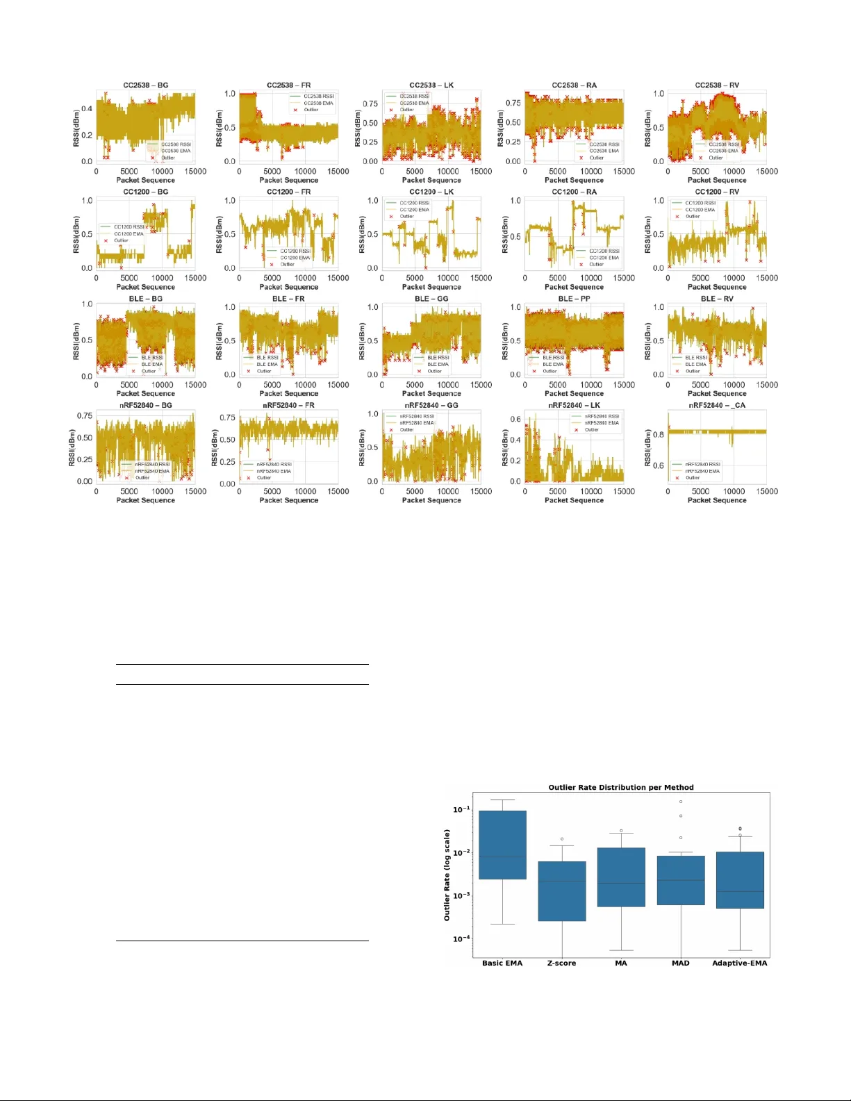
1 A lightweight Outlier Detection for Characterizing Radio- and En vironment-Specific Link Quality Fluctuation in Lo w-Po wer W ireless Networks Zege ye Mekasha Kidane , W altenegus Dar gie , Senior Member , IEEE Abstract —The performance of low-power wireless sensing networks can be influenced by both external en vironmental factors and internal imperfections which often arise due to manufacturing tolerance during mass production. Understanding the conditions and extent of these influences is important not only to achieve high perf ormance and high energy efficiency , but also to carry our en vironment and radio specific configurations. In this paper we demonstrate, through extensi ve practical deployments and experiments, the extent to which exter nal and internal factors affect the link quality of low-power wir eless sensor networks. Moreo ver , we propose a lightweight statistical outlier detection technique and define all the parameter thereof in terms of the statistics of both the raw and the predicted link quality metrics (RSSI). Our study considers more than 15 differ ent physical en vironments consisting of rivers, lakes, bridges, for ests, and gardens, as well as four widely employed heterogeneous low- power radios. Index T erms —Deployment, Internet of Things (IoT), link quality fluctuation, low-power radios, Received Signal Strength Indicator (RSSI), statistical outlier detection, wireless networks I . I N T RO D U C T I O N The wide application of Internet of Things (IoT) in outdoor and semi-outdoor en vironments has increased the demand for resilient low-po wer wireless communication [1], [2]. Appli- cations such as environmental monitoring, smart agriculture, and structural health monitoring rely on resource-constrained sensing devices that must operate in highly dynamic and harsh propagation conditions [3]. In these scenarios, the radios should be fast to predict and react to link quality fluctuations [4]. The Receiv ed Signal Strength Indicator (RSSI) is one of the most widely used metrics for analyzing, estimating, and modeling link quality as well as for adapti ve transmission power control due to its minimal computational and hardware ov erhead [5]–[7]. Nev ertheless, RSSI in lo w-power radios is highly sensitive to en vironmental and internal factors. Outdoor propagation is strongly affected by factors such as v egetation density , terrain irregularity , and water motion, all of which introduce multipath propagation, shado wing, and time-v arying interference. These factors not only lead to significant RSSI fluctuations, b ut also to poorly correlated or even uncorrelated link quality variations. Deployment- and measurement-based Manuscript submitted on March 13. Z. M. Kidane is with Max Planck Institute for Radio Astronomy , 53902 Bad Muenstereifel, Germany (e-mail: zkidane@mpifr-bonn.mpg.de) W . Dargie is with the Faculty of Computer Science, T echnische Uni versit ¨ at Dresden, 01062 Dresden, Germany (waltenegus.dar gie@tu-dresden.de) studies in harsh industrial and outdoor en vironments confirm to this condition, indicating that RSSI instability is the dominant cause of poor link quality characterization and a considerable amount of packet loss in low-po wer wireless networks [8]. Device imperfections and manuf acturing tolerance in mass production of low-po wer radios further exacerbate link quality instability and the dif ficulty to predict and adapt to link quality fluctuations [9], [10]. T o mitigate these concerns, recent research has focused on anomaly and outlier detection, exploring both statistical methods and machine-learning. The former ha ve the adv antage of being computationally af fordable and relativ ely easy to interpret, while the latter of fers improved detection accuracy in highly non-stationary en vironments [11]. Surveys and com- parativ e studies emphasize that anomaly detection is becoming a critical component of reliable IoT system modeling, deploy- ment and configuration, particularly for outdoor and large- scale deplo yments [12], [13]. Howe ver , most existing studies rely on statistics established with the help of homogeneous radio platforms and controlled deployment en vironments (most of which are lab based). In particular , comparati ve experimen- tal analyses that jointly consider radio-specific characteristics, en vironmental variability , and statistical outlier behavior are limited. This paper aims to fill this gap through a comprehensi ve experimental study of RSSI fluctuations in lo w-power wireless networks and statistical outlier detection across heteroge- neous IoT radio platforms deployed in multiple, highly dy- namic outdoor environments. F our different lo w-power radio platforms—CC1200, CC2538, nRF52840, and BLE—and fi ve different outdoor scenarios—bridges, forests, lakes, riv ers, and gardens—are employed in our study . The paper makes the following contributions: (1) Based on extensi ve experiments and data collection, the paper offers practical and useful insight into link quality fluctuation and sensitivity in lo w- power wireless networks. (2) The lightweight statistical outlier detection strate gy we propose enables to isolate correlated link quality fluctuation from uncorrelated (erratic) fluctuation. (3) The sensitivity coefficient we define in the outlier model enables to separately e valuate en vironmental and radio-specific causes to outliers. Overall, the paper addresses the estimation, detection (out- liers), and char acterization aspects of lo w-power wireless links in statistical terms. W e argue that the contributions we stated above enable the deployment of resilient networks as well as en vironment- and radio-specific trade-offs between 2 performance and power consumption. The remaining part of this work is organized as follows. In Section II, we revie w related work. In Section III, we describe node deployment. In Section IV we briefly discuss link quality fluctuation and models for low-po wer wireless deployments. In Section V, we model a wireless link as a random variable and, outliers, as a deviation in the random variable from its mean. The deviation thresholds are expressed in terms of the variance of the random variable as well as a sensiti vity coefficient. In Section VI, we present results based on the statistical ev aluation of a large volume of data we gathered from various physical en vironments using lo w-power wireless sensor networks. Finally , in Section VII, we giv e concluding remarks and outline future work. I I . R E L A T E D W O R K Statistical and machine learning–based outlier detection for RSSI and sensor data has been widely studied across wireless sensor networks (WSNs) and IoT systems. Early statistical approaches, such as Z-score or deviation thresholding, focus on lightweight signal filtering that can operate within the computational limits of sensor nodes [14], [15]. These meth- ods are often well suited for real-time outlier remov al and computational ef ficiency but their usefulness is limited when the data they deal with exhibit high variability . Recent studies have sought to combine statistical filtering with machine learning to improve anomaly detection accuracy and robustness. For example, Y an et al. propose a hybrid outlier detection to process health care data. The proposed ap- proach combines a density-based outlier detection with cluster - ing using K-Nearest Neighbor algorithm to balance computa- tional ef ficiency with detection performance [11]. Other hybrid approaches integrate deep reinforcement learning, supervised classifiers (e.g., random forest), and unsupervised anomaly detectors to further enhance detection in heterogeneous IoT en vironments [16]. Comparativ e analyses of IoT anomaly detection methods examine how supervised and unsupervised learning models— such as random forests, autoencoders, and support vector machines—can be employed for di verse IoT datasets, high- lighting the need for robust preprocessing and scalable ar- chitectures [17]. Hybrid deep learning models combining con volutional and recurrent networks with autoencoders ha ve also been proposed for spatiotemporal- and reconstruction- based anomaly detection in smart en vironment and industrial IoT applications [18]. Surve y articles on anomaly detection in IoT and sensor networks further emphasize the rapid growth of AI-based approaches, including deep learning, reinforcement learning, and semantic context–aw are methods, which are increasingly adopted to capture comple x temporal and spatial relationships in sensor data processing [16]. These surveys also discuss the challenges of balancing detection accuracy , computational cost, and resource constraints inherent to IoT nodes [17], [19]. Similarly , recent research attempts to deal with harsh low- power wireless links by de veloping advanced time-series anomaly detection techniques that could be relev ant for RSSI analysis. Transformer -based architectures for multi variate time series anomaly localization and reconstruction-based mod- els improve detection and localization performance [20]. Representation-based and contrastive learning approaches fur- ther enhance unsupervised time series anomaly detection by modeling temporal and topological patterns [21]. Despite the broad literature on anomaly detection in this conte xt, most existing w ork either focuses on general data or network traffic anomalies or is ev aluated on controlled datasets rather than real outdoor deployments. Fe wer studies specifically address RSSI time series dynamics across heterogeneous radio platforms under di verse outdoor en vironmental conditions, leaving a gap in systematic comparativ e analyses across hardw are types and real-world signal variability . In contrast, our work provides a unified statistical analysis of RSSI fluctuations and outlier patterns across multiple IoT radios deployed in varied outdoor en vironments, integrating classical statistical techniques with lightweight signal process- ing and outlier detection frameworks for resource-constrained systems. I I I . D E P L OY M E N T For our experiments, we employed two widely used sensor node architectures: Zolertia RevB 1 and Adafruit nRF52840 Feather 2 . In the former was installed the Contiki [22] operating system, whereas in the second, the RIOT [23] operating system. The Zolertia Re vB architecture is based on the 32-bit ARM Cortex-M3 processor operating at 32 MHz and integrates two IEEE 802.15.4 compliant low-po wer radios from T exas Instruments: a sub-Gigahertz radio (CC1200 [24]) transmitting at 50 kbps, and a 2.4 GHz radio (CC2538 [25]), transmitting at 250 kbps. The CC1200 has a wide range of operating frequency bands (137-158.3, 164-190, 205-237.5, 274-316.6, 410-475, 820-950 MHz) and a nominal transmission range of about 4 km. The transmission range of the CC2538 is about 100 m. The CC2538 radio had a sensitivity of –97 dBm and an adjustable output power (max. output power = 7 dBm). The sensitivity of the CC1200 radio depends on its transmission rate (–123 dBm at 1.2 kbps and –109 dBm at 50 kbps); its maximum transmission po wer is 16 dBm. For our experiments, the transmission power of both radios was fixed at 0 dBm. The CC2538 radio was configured to transmit 25 packets per second. The CC1200 radio was configured to transmit 3 packets per second at 868.5 MHz. The Adafruit nRF52840 Feather node [26] is a lo w-power , high-performance system-on-chip board with a 32-bit ARM Cortex-M4F processor operating at 64 MHz. It integrates a multiprotocol SoC radio stack which can be configured as Bluetooth Low Ener gy (BLE), Thread, or Zigbee. For our experiments, the radios are configured as follows: • IEEE 802.15.4 mode: 2.4 GHz, nRF52840 transmitted 10 packets per second at 0 dBm with a maximum data rate of 250 kbps. 1 https://doc.riot- os.org/group boards remote- revb .html 2 https://www .adafruit.com 3 • BLE mode: 2.4 GHz, broadcasting 5 packets per second at 0 dBm. T ABLE I N O DE C O N FIG U R A T I O N . Node Radio Frequency Pkt/s Data Rate (kbps) OS Zolertia RevB CC2538 2.4 GHz 25 250 Contiki Zolertia RevB CC1200 Sub-1 GHz 3 1.2 Contiki nRF52840 Feather nRF52840 2.4 GHz 10 250 RIOT nRF52840 Feather BLE 2.4 GHz 5 125 RIO T Our sensor netw orks were deplo yed in 15 different physical en vironments. Some of the nodes were placed inside water - proof boxes to protect them from extreme weather , rain, and/or surface water . A network of 6 Zolertia nodes (with CC2538 and CC1200 radios) was deployed in W est Germany in fiv e different places (on the Rhine Riv er (R V), a small lake (LK), under a bridge (BG), on a forest (FR), and in a residential garden (GG)). The deployment en vironments were chosen because the y represent various real-w orld en vironments. Fig. 1 displays the preparation and deployments of the sensor net- works. The network had a star topology in which fi ve leaf nodes transmitted packets to a sixth central node, which played the role of a sink. The distance between the nodes v aried between 5 to 10 m, depending on the specific deployment en vironment and surrounding objects; the distance on the ri ver and the lake was affected by water motion. Since, we were interested in modeling outliers in individual wireless links, the difference in transmission distance was of secondary concern. During the entire experiments, we made sure that no link was permanently broken. In all the experiments, the antennas were vertically oriented (the nodes employed Herdio Marine waterproof Antennas which were approximately 16 cm high abov e ground or water surface). Upon receiving a packet from its leaf nodes, the sink e xtracted the RSSI and store the data along with a timestamp. For the deployments in the western part of German y , a single experiment lasted about 20 minutes. For each deployment and configuration, we conducted at least fiv e independent experiments on different days under different weather conditions. Like wise, the Adafruit nRF52840 Feather nodes were de- ployed in 10 dif ferent places in the eastern part of Germany (the city of Dresden). T wo dif ferent groups of students carried out the deployments, each group targeting 5 deployment en vironments: the Elbe river , a busy bridge, a forest, a small lake, and a big public park. For these deployments, a network consisted of 3 nodes forming a mesh topology . Here as well, the distance between the sensor nodes varied from 5 to 10 meter , depending on the nature of the deployment en viron- ments. Each node broadcast packets to the other nodes in the network, and each node locally kept a record of the packets it received along with the ID of the transmitter , timestamps, and the RSSI of the received packets. F or the deplo yments in Dresden, the duration of a single experiment was 30 minutes. T able II summarizes the deplo yment in both parts of Germany . I V . W I R E L E S S L I N K Q UA L I T Y In lo w-power wireless sensor networks, the receiv ed signal strength indicator (RSSI) is commonly used as a physical- layer metric for link quality assessment and abnormal behavior T ABLE II S E NS O R N O D E D E PL OY M E NT A C R OS S R A D I O P L A T F OR M S Radio Platform Number of Nodes CC1200 5 CC2538 5 nRF52840 3 BLE 3 detection. The dif ferent radios we employed for our study , despite differences in operating frequency and modulation, share similar RSSI measurement limitations due to lo w-cost and ener gy-efficient hardware design. In general, the receiv ed signal strength (in dBm) at time t can be decomposed into four components: R t = P t − P L ( d ) + D t + η t (1) All the terms on the right hand side are expressed in terms of dBm as well. P t denotes the transmit po wer; P L ( d ) represents large-scale path loss as a function of the distance separating the transmitter and the receiv er; E t captures deployment or en vironment-induced variations, and η t represents stochastic noise and fast fading effects. 1) T ransmit P ower: The transmit po wer P t is constrained and typically selected from a discrete set of hardware- supported levels. For the CC2538 operating at 2.4 GHz under IEEE 802.15.4, P t ranges from − 24 dBm to +7 dBm [25]. The nRF52840 supports both IEEE 802.15.4 and BLE modes at 2.4 GHz, with transmit po wer lev els ranging from − 20 dBm to +8 dBm [26]. The CC1200 operates in the sub-GHz band and supports transmit po wer lev els of up to +14 dBm, depending on the channel and rate configurations [24]. In the BLE mode, the nRF52840 may employ adaptive transmit po wer control. Howe ver , ov er short observation intervals, P t can be assumed quasi-static, and variations in R ( t ) are primarily attributed to propagation and channel effects. 2) Lar ge-Scale P ath Loss: The large-scale path loss term P L ( d ) models the deterministic attenuation of the wireless signal with distance and is commonly e xpressed using the log- distance path loss model: P L ( d ) = P L ( d 0 ) + 10 n log 10  d d 0  (2) where d 0 denotes a reference distance and n is the path loss exponent. Radios operating at 2.4 GHz, including the CC2538 and nRF52840 in both IEEE 802.15.4 and BLE modes, e xperience higher free-space attenuation and increased sensitivity to obstructions and human body shadowing. In contrast, the sub-GHz CC1200 exhibits lower path loss and improv ed penetration, resulting in more stable RSSI beha vior ov er distance [24]. 3) En vironment-Induced V ariations: The term D t accounts for slow-v arying environment-induced ef fects such as shad- owing, reflection, scattering, and temporal variations caused by moving objects or human acti vity . These effects are particularly relev ant in indoor and semi-static deployment scenarios. In BLE, frequency hopping across multiple chan- nels introduces additional v ariability , as individual channels 4 Fig. 1. Prototype deployment in W est German y . From left to right: Sensor nodes in waterproof boxes before deployment. Deployment on a small lake (LK); deployment under Cologne Bridge (BG), along the bridge structure; and deployment on the Rhine Riv er (R V). experience distinct multipath conditions [26]. IEEE 802.15.4 links typically operate at a fixed channel, leading to RSSI variations that are more strongly influenced by local multipath characteristics. For the sub-GHz CC1200, the longer carrier wa velength reduces sensitivity to small-scale obstructions, resulting in smoother temporal RSSI v ariations. 4) Noise and F ast F ading: The term η t represents fast- varying stochastic effects, including thermal noise, receiver front-end noise, fast multipath fading, co-channel interference, and system (manufacturing) imperfections or tolerance. For the CC2538, RSSI values are av eraged ov er multiple symbols, which reduces instantaneous v ariance at the cost of increased measurement latency [25]. The nRF52840 reports RSSI on a per-packet basis in both IEEE 802.15.4 and BLE modes, with BLE measurements being particularly sensitiv e to short packet durations and channel hopping [26]. The CC1200 provides configurable RSSI filtering options, enabling a trade- off between responsiv eness and noise suppression [24]. Due to these factors, η ( t ) is typically modeled as a zero-mean Gaussian random process with variance σ 2 . A. W ide-Sense Stationary Property The condition for a wide-sense stationary stochastic process is that some of the essential statistical features (mean and variance) are inv ariant to times shifts. This condition could be observed in the low-po wer networks we deployed for all the radios, provided that the time interval of interest is in the order or se veral seconds. Fig. 2 shows the histograms of the change in RSSI for the deployment we carried out on the Rhine Riv er using the CC2538 radio (the least reliable, as we shall show). The time windows we considered were 30, 60, 90, 120, and 150 seconds. W ithin these time windows, the statistics of the change in RSSI exhibited no appreciable difference in the shape of the distribution, mean (0.0095, 0.0206, 0.0166, 0.0139, 0.0045) and variance (3.58, 5.48, 4.57, 3.87, 4.47). In the sections that follow , we assume that the stationary condition applies to the outlier detection approach we propose. It is also implied that the time window which concerns us is shorter than 180 seconds. V . M O D E L I N G O U T L I E R S Let R t denote the raw RSSI measurement at a discrete time index t , expressed as a random variable. T o suppress high-frequency noise while preserving the slowly varying propagation trend, we apply an exponential moving av erage ( E t ), equi valent to a first-order causal infinite impulse response (IIR) low-pass filter . Here, the choice of a low-pass filter is deliberate, as outliers are typically erratic, high-frequency variations in the input time series which do not allow mean- ingful system adaptations. The filtered RSSI sequence can be expressed as: E t = α R t + (1 − α ) E t − 1 , 0 < α ≤ 1 (3) with initialization E 0 = R 0 . If we use the Kalman nomencla- ture [27], the first term of the RHS of Equation 3 corresponds to a fresh measurement for time t , and the second term corresponds to a prediction for the same time. From a signal processing perspectiv e, the EMA implements a single-pole low-pass filter whose effecti ve bandwidth is controlled by the smoothing factor α . Smaller v alues of α correspond to stronger attenuation of fast fading and measurement noise, while larger values increase responsi veness to short-term RSSI fluctuations. The EMA output thus serves as an estimate of the underlying mean RSSI component associated with large-scale propagation effects. T ABLE III N OTA T I O N U S ED T H RO U GH O U T E M A S M O OT H IN G A N D R SS I O U TL I E R D E TE C T I ON . Symbol Meaning Units / Notes R t Raw RSSI measurement at time t dBm E t Exponential moving average of RSSI at time t dBm z t abs. dif f between R t and E t − 1 dBm α EMA smoothing factor dimensionless, σ 2 R V ariance of R t (dBm) 2 σ 2 E V ariance of E t (dBm) 2 σ 2 z V ariance of z t (dBm) 2 k Sensitivity parameter for outlier de- tection dimensionless t Discrete time index samples 1 ( · ) Indicator function: 1 if condition true, 0 otherwise dimensionless A. V ariance-based selection of the EMA parameter Under stationary and steady-state conditions, EMA ’ s v ari- ance is related to the v ariance of the input RSSI, R t . Fur- thermore, under the same condition, the RSSI samples can be 5 30swindow RSSI(mdB) -10 0 10 Frequency 0 50 10 0 15 0 20 0 60sw indow RSSI(mdB) -10 0 10 0 50 10 0 15 0 20 0 25 0 30 0 90swindow RSSI (m dB) -10 0 10 0 10 0 20 0 30 0 40 0 120sw indow RSSI (m dB) -10 0 10 0 10 0 20 0 30 0 40 0 50 0 150sw indow RSSI (m dB) -10 0 10 0 10 0 20 0 30 0 40 0 50 0 60 0 Fig. 2. Histograms of ∆ RS SI for fiv e dif ferent time windo ws (Radio: CC2538. Location: Rhine River). regarded as independent and identically distrib uted (i.i.d.) with variance σ 2 R . This leads to the assertion that R t and E t − 1 are statistically independent 3 . Hence: V ar(E t ) = α 2 V ar( R t ) + (1 − α ) 2 V ar(E t − 1 ) + 2 α (1 − α ) Cov( R t , E t − 1 ) (4) Since we assume that R t is statistically independent with all past values, including E t − 1 , the co variance term in Equation 4 is zero. Moreover , under the steady state assumption: V ar( E t ) = V ar( E t − 1 ) = V ar( E ) (5) Consequently , V ar( E ) = α 2 − α V ar( R ) (6) If we let σ 2 R = V ar( R ) and σ 2 E = V ar( E ) , Solving Equation (6) for α yields: α = 2 σ 2 E σ 2 R + σ 2 E (7) Equation (7) shows that the EMA smoothing parameter is directly determined by the ratio of the filtered and unfiltered RSSI variances. A small variance reduction ( σ 2 E ≈ σ 2 R ) results in α → 1 , corresponding to minimal smoothing and high responsiveness. Con versely , a strong variance reduction ( σ 2 E ≪ σ 2 R ) yields α → 0 , indicating aggressiv e low-pass filtering. This v ariance-based formulation provides an intuiti ve and principled mechanism for tuning the EMA. B. Statistical Outlier Detection Chebyshev’ s Inequality [28] serves as the basis for our outlier detection: P {| R t − η R | ≥ ϵ } ≤ σ 2 R ϵ 2 (8) where R t represents link quality fluctuation at time t modeled as a random variable and η R and σ 2 R are its mean and variance, respectiv ely . F or a continuous random v ariable, the probability that the values of the random variable lying outside of the interval specified by the left side term in Equation 8 is gi ven by: P {| R t − η R | ≥ k } = Z η R − ϵ −∞ f ( R ) dR + Z ∞ η R + ϵ f ( R ) dR = Z | R − η R |≥ ϵ f ( R ) dR (9) 3 R t does not contribute to the determination of E t − 1 and the latter does not af fect the future RSSI samples. where f ( R ) is the probability density function of R t and R is the specific value R t can take, with a probability associated with f ( R ) . The v ariance of the random variable is by definition: σ 2 R = Z ∞ −∞ ( R − η R ) 2 f ( R ) dR (10) Since all the terms in the integral of Equation 10 are positi ve and the integral goes from −∞ to ∞ , the follo wing inequality holds: σ 2 R ≥ ϵ 2 Z | R t − η R |≥ ϵ f ( R ) dR (11) Rearranging the terms in Equation 11 yields Chebyshev’ s Inequality , since the integral on the right hand side equals P {| R t − η R | ≥ k } . The inequality sets an upper limit to the probability that the link quality deviates from its mean in terms of a sensiti vity coefficient, k . Considering the sensiti ve nature of R t , applying Chebyshev’ s Inequality on it directly makes outlier modeling highly unstable. Instead we model outlier as the absolute deviation of R t from E t − 1 . If we let: z t = | R t − E t − 1 | (12) W e can now specify the outlier condition for a giv en confi- dence lev el δ = σ 2 z /ϵ 2 , as follows (ref. to Equation 11 4 ): Outlier t = ( 1 , z t ≥ E [ z t ] + ϵ 0 , otherwise (13) Where E [ . ] is the expected value of the function. Since R t and E t − 1 are both random variables, so is z t and it is important to determine its probability density function in order to e v aluate Equation 13. For this task, we have to determine the region of interest in the ( R t , E t − 1 ) plane. C. The Density Function of z t The absolute v alue term in Equation 12 is e v aluated dif- ferently depending on the relativ e magnitudes of the random variables: z t = ( R t − E t − 1 , R t > E t − 1 − R t + E t − 1 , R t ≤ E t − 1 (14) In the following, we determine the probability distribution function of z t first: F ( z ) = P { z t ≤ z } ; once this is 4 Now the random variable of interest is z t ≥ 0 , and the condition of outlier is: P { z t ≥ E [ z t ] + ϵ } = R ∞ η z + ϵ f ( z ) dz ≤ σ 2 z /ϵ 2 . 6 𝑹  = 𝑬  𝑹  > 𝑬  𝑹  ≤ 𝑬  𝑃(𝒛 ≤ 𝑧 , 𝑹  > 𝑬  ) 𝑃(𝒛 ≤ 𝑧 , 𝑹  ≤ 𝑬  ) 𝑹  𝑬  𝑹  𝑬  𝒛 𝒕 = 𝑹  − 𝑬  𝒛 𝒕 = −𝑹  + 𝑬  ( 𝑎 ) ( 𝑏 ) 𝐸  = 𝑧  −𝑅  𝑅  𝐸  = 𝑧  +𝑅  𝑅  Fig. 3. The regions of interest to determine the probability distribution function of z t accomplished, we differentiate F ( z ) with respect to z to determine the probability density function f ( z ) . The density function contains all the information we need about z t . As can be seen in Figure 3, the two cases in Equation 14 are separated by the dashed line R t = E t − 1 . When R t > E t − 1 , the region of interest to determine F ( z ) is depicted in Figure 3 (a). This is the intersection of two e vents, namely , P { z ≤ z } and P { R t > E t − 1 } : F ( z ) = Z ∞ −∞ Z R = z + E −∞ f ( R, E ) dR dE (15) where f ( R, E ) is the joint density function. W e ha ve dropped the time indices in the inte gration and will continue to do so as long as the conte xt is clear . For the case where R t ≤ E t − 1 , the region of interest is depicted in Figure 3 (b). Unlike the previous case, the intersection P { z ≤ z , R t ≤ E t − 1 } is not straightforward to integrate; instead, it is much easier to deal with its complement: P { z > z , R t ≤ E t − 1 } . Hence, F ( z ) = 1 − Z ∞ −∞ Z ∞ R = E − z f ( R, E ) dR dE (16) In order to get f ( z ) , we apply Leibnitz’ s differentiation rule 5 5 Giv en we have a function of two random variables: F ( t ) = Z b ( z ) a ( z ) f ( x, z ) dx dF ( z ) dz = db ( z ) dz f ( b ( z ) , x ) − da ( z ) dz f ( a ( z ) , x ) + Z b ( z ) a ( z ) d f ( x, z ) dz dx on Equations 15 and 16 to obtain the following results 6 : f ( z ) = ( R ∞ −∞ f ( z + E , E ) dE , R t > E t − 1 R ∞ −∞ f ( E − z , E ) dE , R t ≤ E t − 1 (18) If R t and E t − 1 are statistically independent, then Equations 18 becomes: f ( z ) = ( R ∞ −∞ f R ( E + z ) f ( E ) dE , R t > E t − 1 R ∞ −∞ f R ( E − z ) f ( E ) dE , R t ≤ E t − 1 (19) where f R is used to imply the density of R t . From Equa- tion 19 we can conclude that if R t and E t − 1 are normal and independent, then z is also normal. Moreover , When f ( R ) and f ( E ) are normally distrib uted with the same mean, then z t is also normal with zero mean (truncated, of the sort f ( z ) ∼ e − z 2 / 2 σ 2 z , z ≥ 0 ). Its variance is gi ven as: σ 2 z = σ 2 R + σ 2 E (20) Since we now have the variance of z t , we can describe the sensitivity of a wireless link (due either to the environment or the radio) in terms of it. T o do this, we modify the outlier condition in Equation 13 as follo ws: z t ≥ kσ z k σ z = E [ z t ] + ϵ (21) so that: k = E [ z t ] + ϵ σ z (22) 6 For Equation 15: f ( z ) = dF ( z ) dz = Z ∞ −∞ d dz Z z + E ∞ f ( R, E ) dR dE = Z ∞ −∞  1 .f ( z + E , E ) − 0 . + Z z + E ∞ ∂ f ( R, E ) ∂ z dR  dE = Z ∞ −∞ f ( z + E | {z } R , E ) dE (17) 7 Or , in terms of the confidence level, δ , k = E [ z t ] σ z + σ z √ δ ≈ σ z √ δ (23) As can be seen, k is directly proportional to the variance of z t and in versely proportional to the square root of the confidence lev el. For a fix ed confidence le vel, the lar ger the variance of z t , the larger is the sensitivity coefficient, signifying an unstable link. V I . R E S U LT S In this section, we apply the model we propose to analyze the measurements we collected from the various environments using the four low-po wer radios. Our objecti ve is to assess the impact of en vironment vs device imperfection on the wireless links the networks established. A. RSSI Dynamics and Outlier P atterns Figure 4 illustrates the temporal ev olution of RSSI across the fi ve groups of en vironments for all the radio platforms. The observed RSSI dynamics are go verned by a combination of large-scale path loss, medium-scale shado wing, and small- scale fading. En vironments with high structural complexity , notably bridges and forests, exhibit considerable RSSI fluc- tuation. These en vironments introduce persistent multipath propagation and shado wing ef fects, leading to frequent devia- tions from the EMA baseline. Statistical analysis using a one- way ANO V A confirms that RSSI variance dif fers significantly across en vironments for all radios ( p < 0 . 05 ). A one-way ANO V A was performed to assess RSSI v ari- ance across deployment en vironments and radios. Device- lev el performance consistency reflects the consistency of RSSI measurements across multiple radio modules under iden- tical environmental conditions. For a comprehensiv e treat- ment of ANO V A methodology , we refer the reader to [29]. En vironment-level F-statistics as shown in T able IV are considerable (BLE: 149,256; CC1200: 413,499; CC2538: 4,489,917; nRF52840: 147,414), indicating significant dif- ferences in RSSI across environments ( p < 0 . 05 ). A p- value below 0.05 is commonly used to denote statistical significance, meaning there is less than a 5% probability that the observed differences occurred by chance. Therefore, these results are statistically significant, allowing rejection of the null hypothesis. The combination of high F-statistics and low p-values confirms that environmental factors strongly influence RSSI, rather than the observed differences being random fluctuations. Hardware-le vel F-statistics are smaller but still significant (BLE: 1,542.3; CC1200: 3,218.7; CC2538: 12,367.9; nRF52840: 1,434.8) demonstrating high measure- ment repeatability and limited hardware variability . These findings indicate that while en vironmental conditions are the primary dri ver of RSSI variations, hardware differences con- tribute a smaller , measurable effect. The frequency of exceeding threshold v alues in the deploy- ment en vironments suggest that sustained link instability rather than isolated measurement noise are the reason for the strong link quality fluctuations. In contrast, the garden environment T ABLE IV R E GE N E R A T E D F - S TA T I ST I C S F O R R S SI V A R I AN C E A N D R A D IO C O NS I S T EN C Y . d f in R E FE R S T O T H E D E GR E E S O F F R E ED O M W I T HI N G RO U PS . T H E D EG R E E S O F F R EE D O M B E T WE E N G RO U P S E QU A LS 4 . Radio Analysis Lev el F-Statistic df in BLE En v . 149,256 89,876 BLE Device 1,542 89,876 CC1200 En v . 413,499 89,166 CC1200 Device 3,219 89,166 CC2538 En v . 4,489,917 812,511 CC2538 Device 12,368 812,511 nRF52840 Env . 147,414 691,018 nRF52840 Device 1,435 691,018 demonstrates relativ ely stable RSSI dynamics with low vari- ance. Near line-of-sight conditions and moderate obstruction allow the EMA to closely track the raw RSSI signal, resulting in a significantly lo wer outlier rate ( p < 0 . 01 ). This character- istic highlights the impact of en vironmental openness on signal stability . Lake and river en vironments exhibit intermediate RSSI dynamics. While open water surfaces generally fa vor stable propagation, intermittent reflections and surface-induced scattering produce sporadic RSSI de viations. These deviations appear as isolated outliers rather than continuous instability , which is reflected in moderate outlier rates of the detection. Across all environments, radio-specific characteristics fur- ther exacerbate RSSI dynamics. CC1200 radios exhibit smoother RSSI trajectories and fewer e xtreme deviations, sug- gesting higher robustness to en vironmental variability . Con- versely , nRF52840 and BLE radios sho w increased sensiti vity to multipath en vironments, resulting in higher outlier rates. These observ ations demonstrate that RSSI dynamics and out- lier patterns are jointly influenced by en vironmental conditions and radio hardware characteristics. B. Comparison of Radio Outlier Rates T o assess the outlier rates for each radio and deployment en vironment, we set the confidence lev el to δ = 0 . 05 . This means that at a confidence coefficient of 0.95, the fluctuation in link quality modeled by the random v ariable z t is considered normal. As mentioned at the end of the previous section, a larger v alue of k indicates higher sensitivity (a link that is prone to outliers). The Outlier Rate comparison highlights distinct differences in performance consistency among the radios. The CC1200 and nRF52840 radios exhibit the lo west outlier rates across all en vironments, often near zero, indicating relatively stable and reliable operation. BLE radios show moderate outlier rates, with the highest observed in the riv er deployments (0.015), suggesting occasional instability under certain conditions. The CC2538 radios ha ve slightly higher and more variable outlier rates compared to CC1200 and nRF52840, although the rates remain generally lo w . Considering α and k alongside outlier rates, it is evident that radios with high α and low k , such as nRF52840, produce fe wer outliers, while radios with higher variability , such as BLE and CC2538, e xperience more frequent de viations. Overall, nRF52840 and CC1200 provide the most consistent performance, BLE is moderately reliable, 8 Fig. 4. Normalized RSSI v ariations in the 15 deployment environments using the four low-po wer radios. The red crosses mark the detected RSSI outliers. and CC2538 is comparatively less stable in terms of outlier occurrences. This is summarized in T able V. T ABLE V O U TL I E R R A T E R A T E S F O R A L L R A DI O S A N D D E P LO YM E N T E N VI RO N M E NT S I N T E RM S O F α A N D k . Radio En v Outlier Rate α k BLE BG 0.007 0.775 3.367 BLE FR 0.016 0.834 3.304 BLE GG 0.014 0.934 3.220 BLE PP 0.004 0.624 3.522 BLE R V 0.011 0.770 3.372 CC1200 BG 0.012 0.950 3.201 CC1200 FR 0.017 0.950 3.192 CC1200 LK 0.007 0.950 3.192 CC1200 RA 0.012 0.950 3.192 CC1200 R V 0.014 0.950 3.200 CC2538 BG 0.005 0.599 3.516 CC2538 FR 0.008 0.601 3.498 CC2538 LK 0.011 0.597 3.510 CC2538 RA 0.002 0.594 3.552 CC2538 R V 0.013 0.602 3.499 nRF52840 BG 0.019 0.950 3.191 nRF52840 FR 0.022 0.950 3.194 nRF52840 GG 0.024 0.950 3.194 nRF52840 LK 0.026 0.950 3.191 nRF52840 CA 0.009 0.950 3.189 C. Comparison with Baselines In this section we compare the performance of our approach (Adaptiv e EMA) with four baseline outlier detection methods: Basic EMA (our approach with a fixed α as a threshold), interval estimation based on z-score, Mo ving A verage, Median Absolute Deviation (MAD), and Adaptiv e EMA (our ap- proach). Figure 5 displays the distrib ution of outlier detection rates aggre gated for the four radios and the fifteen deployment en vironments. The v ertical axis is represented on a logarithmic scale to allo w visualization of detection rates spanning sev eral orders of magnitude. In each boxplot, the central horizontal line indicates the median v alue, the box boundaries represent the first and third quartiles (Q1 and Q3), and the whiskers extend to the typical minimum and maximum values, while individual points denote extreme observ ations. Fig. 5. Distribution of outlier detection rates for fiv e anomaly detection methods across four radio platforms and fifteen environmental scenarios. Basic EMA exhibits the highest median detection rate, 9 approximately 10 − 2 , with a wide interquartile range and whiskers extending close to 10 − 1 . This indicates high sensi- tivity b ut also substantial v ariability , suggesting potential ov er- detection or false positiv es. In contrast, z-score— z t = ( R t − η x ) /σ x ) —shows the lowest median and narrowest spread near 10 − 3 , reflecting a conservati ve detection minimizing false positiv es but risking missing subtle anomalies. Moving A verage lies between z-score and Basic EMA, with moderate median values and a wider spread than z-score, capturing more anomalies while maintaining moderate stability . MAD has a similar median to MA but features sev eral extreme outliers, indicating occasional high detection rates and higher variability in some scenarios. Finally , Adapti ve EMA (outlier threshold = k σ z ) maintains a median detection rate comparable to MA and MAD b ut with a narro wer interquartile range and fewer extreme v alues. This demonstrates a balanced trade- off between sensiti vity and stability , enabled by its dynamic smoothing adjustment. Overall, Adapti ve EMA deli vers more consistent and reliable anomaly detection across varying ra- dios and en vironments, outperforming the other methods in robustness and statistical stability . V I I . C O N C L U S I O N This paper presented a comprehensi ve experimental analysis of RSSI fluctuations and statistical outlier behavior across heterogeneous IoT radio platforms deployed in div erse outdoor en vironments. By integrating a mathematical RSSI abstraction with exponential moving av erage (EMA) smoothing and sta- tistically grounded outlier detection, the study examined ho w en vironmental complexity and radio hardware characteristics jointly influence signal stability . Experimental results sho wed that en vironments with high structural and propagation com- plexity exhibit higher RSSI variance and increased outlier occurrence compared to more open en vironments such as gardens. The proposed outlier detection provides a compact and interpretable representation of RSSI anomalies, enabling systematic comparison across radio platforms and deployment scenarios. Among the e valuated radios, the CC1200 consis- tently demonstrates the greatest rob ustness to en vironmental variability . The nRF52840 also exhibits high o verall stability but sho ws increased sensiti vity in multipath-rich en vironments, while BLE and CC2538 radios display moderate and more variable performance. These findings provide practical insights for IoT and sensor network designers, supporting informed radio selection, en vironment-aware deployment planning, and adaptiv e communication strategies. The lightweight nature of the proposed framework makes it well suited for resource- constrained IoT devices and long-term outdoor monitoring applications, where predictable link behavior is essential. Future work will explore adaptive thresholding tech- niques, multi-metric link-quality fusion, and machine learn- ing–assisted anomaly classification to further enhance rob ust- ness under highly dynamic propagation conditions. R E F E R E N C E S [1] Z. Chen, Y . Gao, and J. Liang, “Lopdm: A low-power on-device pre- dictiv e maintenance system based on self-powered sensing and tinyml, ” IEEE T ransactions on Instrumentation and Measur ement , vol. 72, pp. 1–13, 2023. [2] M. Chaudhary , N. Goyal, A. Benslimane, L. K. A wasthi, A. Alwadain, and A. Singh, “Underwater wireless sensor networks: Enabling technolo- gies for node deployment and data collection challenges, ” IEEE Internet of Things Journal , vol. 10, no. 4, pp. 3500–3524, 2022. [3] S. Rani, H. Babbar , P . Kaur , M. D. Alshehri, and S. H. Shah, “ An optimized approach of dynamic target nodes in wireless sensor network using bio inspired algorithms for maritime rescue, ” IEEE T ransactions on Intelligent T ransportation Systems , vol. 24, no. 2, pp. 2548–2555, 2022. [4] H. Kim, H.-S. Kim, and S. Bahk, “Mobirpl: Adaptive, robust, and rssi- based mobile routing in low power and lossy networks, ” Journal of Communications and Networks , v ol. 24, no. 3, pp. 365–383, 2022. [5] W . Dargie, “Prediction of recei ved power in low-po wer and lossy networks deployed in rough en vironments, ” IEEE T ransactions on Instrumentation and Measurement , 2025. [6] J. Tian, L. Cong, H. Qin, and Y . W ang, “Environmental landmark-based loop closure detection combining fm/wifi/magnetic field signals for indoor slam, ” IEEE T ransactions on Instrumentation and Measurement , 2025. [7] K. Srini vasan, P . Dutta, A. T avak oli, and P . Levis, “ An empirical study of low-po wer wireless, ” ACM T ransactions on Sensor Networks (TOSN) , vol. 6, no. 2, pp. 1–49, 2010. [8] T . Prasayasith, P . Saengudomlert, and W . S. Mohammed, “Performance ev aluation and improvement of wireless rssi based animal theft detec- tion, ” ECTI T ransactions on Electrical Engineering, Electr onics, and Communications , v ol. 21, no. 3, 2023. [9] M. Letafati, A. Kuhestani, and H. Behroozi, “Three-hop untrusted relay networks with hardware imperfections and channel estimation errors for internet of things, ” IEEE T ransactions on Information F orensics and Security , v ol. 15, pp. 2856–2868, 2020. [10] Y . Liu, J. W ang, J. Li, S. Niu, and H. Song, “Machine learning for the detection and identification of internet of things devices: A survey , ” IEEE Internet of Things Journal , v ol. 9, no. 1, pp. 298–320, 2021. [11] K. Y an, X. Y ou, X. Ji, G. Yin, and F . Y ang, “ A hybrid outlier detection method for health care big data, ” in 2016 IEEE International Confer - ences on Big Data and Cloud Computing (BDCloud), Social Computing and Networking (SocialCom), Sustainable Computing and Communica- tions (SustainCom) (BDCloud-SocialCom-SustainCom) , 2016, pp. 157– 162. [12] D. Adhikari, W . Jiang, J. Zhan, D. B. Rawat, and A. Bhattarai, “Recent advances in anomaly detection in internet of things: Status, challenges, and perspectives, ” Computer Science Review , vol. 54, p. 100665, 2024. [13] L. A. Mu ˜ noz, J. V . Bern ´ a Mart ´ ınez, F . Maci ´ a P ´ erez, and I. Lorenzo Fon- seca, “ Anomaly detection system for data quality assurance in IoT infrastructures based on machine learning, ” Internet of Things , vol. 25, p. 101095, 2024. [14] J. Xiao, L. Y ang, F . Zhong, X. W ang, H. Chen, and D. Li, “Robust anomaly-based insider threat detection using graph neural network, ” IEEE T ransactions on Network and Service Management , vol. 20, no. 3, pp. 3717–3733, 2022. [15] A. S. Y aro, F . Maly , P . Prazak, and K. Mal ´ y, “Outlier detection performance of a modified z-score method in time-series rss observation with hybrid scale estimators, ” IEEE Access , vol. 12, pp. 12 785–12 796, 2024. [16] S. W ali, M. I. Khan, and M. Imran, “Semantic-aware reinforcement and ensemble learning for signal management and anomaly detection in IoT systems, ” Scientific Reports , 2025. [17] Z. A. Haider, A. Zeb, T . Rahman, S. K. Singh, R. Akram, A. Arishi, and I. Ullah, “ A survey on anomaly detection in IoT: T echniques, challenges, and opportunities with the inte gration of 6g, ” Computer Networks , vol. 270, p. 111484, 2025. [18] T . Deng, H. Li, and C. Ni, “Time series anomaly detection methods for IoT in smart grids: A systematic review , ” Neurocomputing , vol. 661, p. 131967, 2025. [19] D. Li, N. Nair, and K. W ang, “Unsupervised time series anomaly detection for edge computing: A review , ” in IoT Edge Intelligence . Springer , 2024, pp. 173–198. [20] Z. Chen, D. Chen, X. Zhang, Z. Y uan, and X. Cheng, “Learning graph structures with transformer for multivariate time-series anomaly detection in iot, ” IEEE Internet of Things Journal , v ol. 9, no. 12, pp. 9179–9189, 2021. [21] S.-M. V ilhes, G. Gasso, and M. Z. Alaya, “Patchtrad: A patch-based transformer for time series anomaly detection, ” arXiv preprint , 2025. [22] G. Oikonomou, S. Duquennoy , A. Elsts, J. Eriksson, Y . T anaka, and N. Tsiftes, “The contiki-ng open source operating system for next generation IoT devices, ” SoftwareX , vol. 18, p. 101089, 2022. 10 [23] E. Baccelli, C. G ¨ undo ˘ gan, O. Hahm, P . Kietzmann, M. S. Lenders, H. Petersen, K. Schleiser, T . C. Schmidt, and M. W ¨ ahlisch, “Riot: An open source operating system for low-end embedded devices in the IoT, ” IEEE Internet of Things Journal , v ol. 5, no. 6, pp. 4428–4440, 2018. [24] T exas Instruments, CC1200 High-P erformance RF T ransceiver , T exas Instruments, 2023. [25] ——, CC2538 System-on-Chip Solution for 2.4-GHz IEEE 802.15.4 , T exas Instruments, 2023. [26] Nordic Semiconductor, nRF52840 Multipr otocol SoC , Nordic Semicon- ductor , 2023. [27] R. E. Kalman, “ A ne w approach to linear filtering and prediction problems, ” 1960. [28] A. P apoulis and S. U. Pillai, Pr obability . McGraw-hill, 2002. [29] D. C. Montgomery , Design and Analysis of Experiments , 9th ed. Hoboken, NJ, USA: John Wile y & Sons, Inc., 2022.