Power Bounds and Efficiency Loss for Asymptotically Optimal Tests in IV Regression

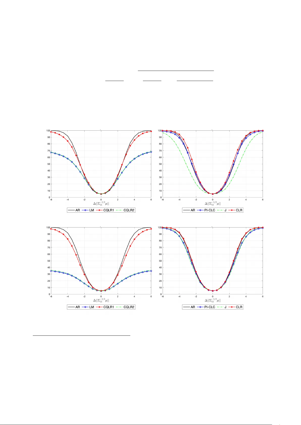
P o w er Bounds and Efficiency Loss for Asymptotically Optimal T ests in IV Regression ∗ Marcelo J. Moreira Geert Ridder Mahrad Sharifv aghefi Marc h 24, 2026 Abstract W e c haracterize the maximal attainable pow er–size gap in ov eriden tified instrumen- tal v ariables mo dels with heteroskedastic or auto correlated (HA C) errors. Using total v ariation distance and Kraft’s theorem, we define the decision theoretic frontier of the testing problem. W e show that Lagrange multiplier and conditional quasi likelihoo d ratio tests can ha ve pow er arbitrarily close to size even when the n ull and alternative are w ell separated, b ecause they do not fully exploit the reduced-form lik eliho o d. In con trast, the conditional likelihoo d ratio (CLR) test uses the full reduced-form lik eliho o d. W e pro ve that the p ow er–size gap of CLR conv erges to one if and only if the testing problem b e- comes trivial in total v ariation distance, so that CLR attains the decision theoretic fron tier whenev er an y test can. An empirical illustration based on Y ogo (2004) shows that these failures arise in empirically relev an t configurations. Keywor ds: Endogenous regressor, Instrumen tal v ariable, Conditional lik eliho o d ratio test, Lagrange Multiplier test, HAC errors, T otal v ariation distance JEL classific ation: C14, C36 ∗ This paper supersedes the corresponding sections of the previous working paper “Efficiency Loss of Asymptotically Efficient T ests in an Instrumen tal V ariables Regression” and the note “Po wer of the CLR T est and T otal V ariation Distance in an Instrumental V ariables Regression” by the same set of authors. 1 1 In tro duction This pap er studies the p ow er–size tradeoff in instrumen tal v ariable mo dels under w eak iden- tification and heteroskedastic or auto correlated (HA C) errors. W e characterize the in trinsic difficult y of the testing problem using total v ariation distance and derive the maximal attain- able p o w er–size gap, whic h defines the decision theoretic frontier for the problem. W e then study whether commonly used w eak-identification-robust pro cedures attain this frontier. In particular, we sho w that the conditional lik eliho o d ratio (CLR) test attains this fron tier when- ev er an y test can do so, whereas Lagrange multiplier (LM) and conditional quasi likelihoo d ratio (CQLR) tests ma y fail to attain it in HA C environmen ts. Inference in instrumental v ariable mo dels is complicated b y weak identification. The test of Anderson and Rubin (1949) w as the first pro cedure shown to remain v alid when instruments are arbitrarily weak b ecause its n ull distribution does not dep end on instrument strength. How ever, the Anderson Rubin (AR) test is not efficient under the usual strong instrument asymptotics. This inefficiency motiv ated the developmen t of pro cedures that retain robustness to weak iden tification while achieving asymptotic efficiency when instrumen ts are strong. Standard W ald and lik eliho o d ratio tests are efficient under strong instruments but can exhibit sev ere size distortions when instruments are w eak; see Nelson and Startz (1990), Dufour (1997), Staiger and Sto ck (1997), and W ang and Ziv ot (1998). These distortions arise b ecause their n ull distri- butions dep end on first-stage co efficients when instrumen ts are w eak. A conditioning argumen t resolv es this problem b y replacing the usual chi–square critical v alue with a null quantile con- ditional on a statistic sufficien t for the first-stage co efficients, as prop osed b y Moreira (2003). The resulting conditional W ald (CW) and conditional lik eliho o d ratio (CLR) tests, together with the LM test, are asymptotically efficient under strong identification and v alid under weak iden tification. In homoskedastic mo dels these pro cedures hav e well-understoo d prop erties. Andrews, Mor- eira, and Sto c k (2007) sho w that CW can exhibit severe p ow er distortions under w eak identifi- cation. In con trast, LM and CLR are un biased and efficient under strong identification. In this setting, the efficiency gain relative to AR do es not compromise asymptotic p ow er prop erties, as Andrews, Moreira, and Stock (2004, 2006) establish that both LM and CLR are consis- 2 ten t. Ho w ever, these results do not determine whether existing procedures fully exploit the information av ailable in more general en vironmen ts. The situation c hanges in ov eridentified mo dels with heterosk edastic or auto correlated errors. In these mo dels the reduced-form cov ariance structure contains information that is not fully exploited by tests constructed from AR and LM statistics. T ests designed to improv e up on AR can therefore lose p o wer for reasons that do not arise under homoskedasticit y . W e show that this loss of information can b e structural rather than lo cal. In instrumental v ariable mo dels with heterosk edastic or auto correlated errors the reduced- form co v ariance matrix in tro duces man y n uisance parameters. When the num b er of instruments increases, the num b er of cov ariance parameters gro ws roughly with the square of the n um b er of instruments, making the testing problem inheren tly high dimensional. Classical p ow er com- parisons, suc h as those of Andrews, Moreira, and Sto c k (2006), dep end on a small n umber of parameters even when the n umber of instrumen ts increases. In con trast, the HAC IV frame- w ork allo ws a muc h richer set of co v ariance configurations. Sho wing that pow er failures arise in such a rich environmen t is therefore not straigh tforward. Our first con tribution is to c haracterize the maximal attainable p o wer–size gap using the total v ariation distance b et ween the n ull and alternativ e distributions. Bertanha and Moreira (2020) sho w that total v ariation distance is the relev an t metric for determining whether an y test can deliver non trivial p ow er. By Kraft (1955), the minim um total v ariation distance b et w een the con vex hulls of the n ull and alternativ e models determines the largest p o w er–size gap ac hiev able b y an y measurable test. W e deriv e an explicit b ound for this frontier in the linear IV mo del and show that it pro vides a necessary and sufficient condition for asymptotic distinguishability . W e then show that the p o wer–size gap of the conditional likelihoo d ratio (CLR) test con- v erges to one if and only if the decision theoretic fron tier conv erges to one. Thus, CLR attains the maximal attainable p o w er–size gap whenev er an y test can do so. This result reflects the fact that CLR exploits the full reduced-form information a v ailable in the HAC mo del. It is useful to contrast this prop erty with existing pro cedures. AR also attains the frontier, although it is not efficien t under strong iden tification. The LM test and the CQLR test w ere dev elop ed to impro ve up on AR while preserving robustness to w eak identification. The CQLR test can b e view ed as an HAC extension of CLR following Kleib ergen (2005). How ever, the t w o 3 pro cedures are not equiv alen t in HA C en vironmen ts. CQLR is constructed from statistics based on AR and LM components, whereas CLR is defined directly from the Gaussian reduced-form lik eliho o d; see Andrews and Mikushev a (2016) and Moreira and Moreira (2019). Consequently , CQLR may discard information con tained in the reduced-form co v ariance structure that CLR fully exploits. W e iden tify a class of data generating pro cesses, which we call imp ossibility designs , under whic h the LM noncentralit y parameter remains b ounded even when the null and alternativ e distributions are arbitrarily well separated. In such designs LM and CQLR can b e inconsisten t, with p o wer arbitrarily close to size. This phenomenon has no analog in the homoskedastic case. These designs are not pathological. The set of data generating pro cesses that generate b ounded noncen tralit y parameters has p ositive measure, and the asso ciated p o wer losses extend to neighborho o ds of these designs. Using data of Y ogo (2004), w e show that empirically plausible parameter configurations can lie near this region. In such cases AR–LM based conditional pro cedures can suffer substan tial p ow er losses, whereas CLR maintains high pow er. T ak en together, our results establish a sharp separation b etw een CLR and b oth LM and CQLR tests in instrumental v ariable mo dels with HA C errors. CLR exploits the full reduced- form likelihoo d and achiev es the decision theoretic fron tier, whereas LM and CQLR op erate in a restricted information space and may fail to conv ert statistical separation into p ow er. Dufour (1997), building on Gleser and Hw ang (1987), sho ws that con v entional W ald tests can hav e size arbitrarily close to one when instrumen ts are arbitrarily weak. This finding supp orted the use of the AR test and the developmen t of other pro cedures robust to weak instrumen ts. Our results rev eal a parallel issue for p ow er in HA C IV mo dels. When the co v ariance structure is near an imp ossibility design, LM and CQLR tests can hav e p ow er arbitrarily close to size even though the n ull and alternativ e distributions are w ell separated. Just as Bound, Jaeger, and Baker (1995), Dufour (1997), and Staiger and Sto c k (1997) shifted empirical practice aw ay from W ald tests tow ard pro cedures robust to weak instruments, our results suggest that procedures based on AR and LM statistics may discard relev an t information in HAC environmen ts. This motiv ates the use of pro cedures such as the CLR test that exploit the full reduced-form likelihoo d and also encourages the developmen t of new tests that fully use the information a v ailable in the reduced-form. 4 The remainder of the pap er is organized as follo ws. Section 2 introduces the mo del and test statistics. Section 3 studies the CLR test using total v ariation distance. Section 4 c haracterizes the noncentralit y parameter of the LM statistic and defines imp ossibilit y designs for both LM and CQLR tests. Section 5 provides diagnostics and an empirical application. Section 6 concludes the pap er. An online supplement contains the pro ofs of all theoretical results, additional lemmas and a prop osition, further p ow er comparisons, and supplementary results for the empirical application. 2 Mo del and test statistics W e consider the instrumental v ariable regression mo del y 1 = y 2 β ∗ + u, (2.1) y 2 = Z π + v 2 , (2.2) where y 1 and y 2 are n × 1 v ectors, Z is an n × k matrix of nonrandom instruments with full column rank, and π is a k × 1 vector of first stage co efficients. F or simplicity w e omit additional cov ariates. They can b e partialled out using orthogonal pro jections according to the F risch–W augh–Lo vell (FWL) theorem; see Andrews, Moreira, and Sto c k (2006) for the IV mo del. The disturbances u and v 2 ha ve mean zero and may exhibit heterosk edasticity and auto correlation. Our ob jective is to test H 0 : β ∗ = β 0 against H 1 : β ∗  = β 0 , treating π as a n uisance parameter. Let Y = [ y 1 y 2 ]. The reduced form can b e written as Y = Z π a ∗′ + V , (2.3) where a ∗ = ( β ∗ , 1) ′ and V = [ v 1 v 2 ] with v 1 = u + β ∗ v 2 . 5 Define R = ( Z ′ Z ) − 1 / 2 Z ′ Y = µa ∗′ + e V , (2.4) where µ = ( Z ′ Z ) 1 / 2 π and e V = ( Z ′ Z ) − 1 / 2 Z ′ V . W e imp ose the following normalized a verage conditions. Assumption NA. (a) n − 1 Z ′ Z → D , where D is p ositive definite. (b) n − 1 V ′ V p → Ω, where Ω is p ositive definite. (c) ( Z ′ Z ) − 1 / 2 Z ′ V d → N (0 , Σ), where Σ is p ositive definite. Under Assumption NA, the finite dimensional distribution of R conv erges to a Gaussian limit exp erimen t with co v ariance matrix Σ. This limit exp erimen t coincides with the w eak instrumen t asymptotics of Staiger and Sto c k (1997) and pro vides a sharp approximation to finite-sample b ehavior when first-stage co efficients are local to zero. It also forms the basis for our fixed-alternative comparisons in later sections. Accordingly , we conduct our analysis under the Gaussian reduced-form mo del R ∼ N ( µa ∗′ , Σ) , (2.5) treating Σ as kno wn. This formulation isolates the information conten t of the reduced form and allows us to analyze the geometry of the testing problem directly . Fix β 0 and define a 0 = ( β 0 , 1) ′ , b 0 = (1 , − β 0 ) ′ . Define T =  ( a ′ 0 ⊗ I k )Σ − 1 ( a 0 ⊗ I k )  − 1 / 2 ( a ′ 0 ⊗ I k )Σ − 1 v ec( R ) , (2.6) S = [( b ′ 0 ⊗ I k )Σ( b 0 ⊗ I k )] − 1 / 2 ( b ′ 0 ⊗ I k )v ec( R ) . (2.7) Under H 0 , T is sufficien t for µ , while S is pivotal and independent of T . 6 Let B 0 =   1 0 − β 0 1   , R 0 = RB 0 . Then v ec( R 0 ) ∼ N (v ec( µa ′ ∆ ) , Σ 0 ) , where a ∆ = (∆ , 1) ′ with ∆ = β ∗ − β 0 and Σ 0 = ( B ′ 0 ⊗ I k )Σ( B 0 ⊗ I k ) =   Σ 11 Σ 12 Σ 21 Σ 22   . The Anderson Rubin statistic is AR = S ′ S. (2.8) The one-sided and t w o-sided LM statistics are LM 1 = S ′ Σ − 1 / 2 11 (Σ 22 ) − 1 / 2 T    Σ − 1 / 2 11 (Σ 22 ) − 1 / 2 T    , LM =  S ′ Σ − 1 / 2 11 (Σ 22 ) − 1 / 2 T  2 T ′ (Σ 22 ) − 1 / 2 Σ − 1 11 (Σ 22 ) − 1 / 2 T , (2.9) where Σ 22 = (Σ 22 − Σ 21 Σ − 1 11 Σ 12 ) − 1 . (2.10) Another commonly used statistic is the quasi likelihoo d ratio (QLR): QLR = AR − r ( T ) + p ( AR − r ( T )) 2 + 4 LM r ( T ) 2 , (2.11) where natural choices for the rank statistic r ( T ) are r 1 ( T ) = T ′ T and r 2 ( T ) = T ′ (Σ 22 ) − 1 / 2 Σ − 1 11 (Σ 22 ) − 1 / 2 T , as outlined by Andrews and Guggenberger (2017). W e refer to these v ariants as QLR 1 and QLR 2. The n ull distribution of QLR dep ends on µ . Since T is sufficien t for µ under H 0 , w e follo w the conditioning argumen t of Moreira (2003) and define conditional versions that reject the n ull hypothesis when the statistic exceeds its n ull quantile conditional on T . The conditional 7 critical v alue function based on a statistic ψ is c α ( T ) = min  c : sup ∆=0 , µ  =0 Pr( ψ > c | T ) ≤ α  . (2.12) W e refer to this as the conditional QLR (CQLR) test. Andrews (2016) sho ws that CQLR is a sp ecial case of conditional linear combination (CLC) tests of the form LC = w ( T ) · AR + (1 − w ( T )) · LM , (2.13) where 0 ≤ w ( T ) ≤ 1 and prop oses the plug-in conditional linear combination test (PI-CLC). Finally , follo wing Moreira (2003) for the homosk edastic case, Andrews and Mikushev a (2016) and Moreira and Moreira (2019) define the likelihoo d ratio statistic for the HAC case: LR = Q ( β 0 ) − inf β ∈ R Q ( β ) , (2.14) where Q ( β ) = vec( R ) ′ ( b ⊗ I k ) [( b ′ ⊗ I k )Σ( b ⊗ I k )] − 1 ( b ′ ⊗ I k )v ec( R ) , (2.15) with b = (1 , − β ) ′ . The conditional likelihoo d ratio (CLR) test rejects when LR exceeds its null quantile con- ditional on T . CQLR extends the algebraic structure of CLR from the homoskedastic setting to the GMM framew ork with heteroskedastic or auto correlated errors, whereas CLR is defined directly from the Gaussian reduced-form lik eliho o d. The tw o pro cedures coincide under homoskedasticit y but are generally distinct in HAC en vironments. When k > 2 in HAC settings, the likelihoo d ratio statistic do es not admit a closed-form solution to the minimization problem in (2.14). Moreira, New ey , and Sharifv aghefi (2024) establish this result and develop computational algebra metho ds that allo w the CLR statistic to b e computed reliably in suc h en vironmen ts. 8 3 CLR test In this section, w e sho w that the p o w er–size gap of the CLR test, which rejects the n ull hy- p othesis when the LR statistic defined in (2.14) exceeds its conditional critical v alue giv en b y (2.12), conv erges to one as the minimum total v ariation distance betw een the con vex h ulls of the distributions under the n ull and alternative hypotheses for R 0 con verges to one. By Kraft (1955)’s theorem, discussed b elo w, this result implies that the p ow er–size gap of an y test can con verge to one only if the same holds for the CLR test. T o place Kraft (1955)’s theorem in the con text of linear IV mo dels, let ϕ ∆ ,µ ( · ) denote the normal probabilit y density function of v ec( R 0 ) with mean v ec( µa ′ ∆ ) and v ariance matrix Σ 0 . Denote the conv ex hull of the set of normal densities under the n ull h yp othesis by C 0 = ( m X i =1 c i ϕ 0 ,µ i ( · ) : c i ≥ 0 , m X i =1 c i = 1 , m ∈ N ) . (3.16) Similarly , let C 1 = ( m X j =1 c j ϕ ∆ j ,µ j ( · ) : c j ≥ 0 , m X j =1 c j = 1 , ∆ 2 j µ ′ j Σ − 1 11 µ j ≥ d, m ∈ N ) (3.17) denote the conv ex hull of the set of normal densities under the alternative h yp othesis satisfying ∆ 2 µ ′ Σ − 1 11 µ ≥ d, (3.18) where d > 0 is an arbitrary constan t. The separation condition in (3.17) reflects the intrinsic statistical distance b et w een the null and alternative distributions in the Gaussian reduced-form mo del. The scalar ∆ 2 µ ′ Σ − 1 11 µ is cen tral for three reasons. First, it equals the noncentralit y parameter of the Anderson–Rubin statistic under the alternativ e, measuring the structural deviation ∆ scaled by instrument strength as summarized b y µ ′ Σ − 1 11 µ . Th us alternativ es satisfying ∆ 2 µ ′ Σ − 1 11 µ ≥ d are separated from the null by at least a fixed AR signal. Second, as sho wn b elo w, a useful bound for the total v ariation distance ov er nuisance mean vectors under the n ull dep ends only on this scalar, so it 9 directly indexes intrinsic distinguishability betw een the null and alternative mo dels. Third, it has a natural econometric interpretation: ∆ 2 = ( β ∗ − β 0 ) 2 is the squared structural distance from the n ull, while µ ′ Σ − 1 11 µ summarizes instrumen t strength. Their pro duct therefore measures structural separation scaled by instrument relev ance. F or these reasons, defining the alternative con vex hull through ∆ 2 µ ′ Σ − 1 11 µ ≥ d provides a mo del-based and decision theoretic notion of separation that allows a sharp characterization of the maximal attainable pow er–size gap. The total v ariation (TV) distance b etw een f ( · ) ∈ C 0 and g ( · ) ∈ C 1 is defined as D TV ( f , g ) = 1 2 Z R 2 k | f ( r 0 ) − g ( r 0 ) | dr 0 . (3.19) Kraft (1955) shows that, in order for there to exist a test ψ ( · ) : R 2 k → [0 , 1] suc h that inf g ∈C 1 E g ( ψ ( R 0 )) − sup f ∈C 0 E f ( ψ ( R 0 )) ≥ q , (3.20) it is necessary and sufficient that min f ∈C 0 g ∈C 1 D TV ( f , g ) = q . (3.21) That is, the p ow er–size gap of a test can b e at least q if and only if the minimum total v ariation distance b etw een C 0 and C 1 equals q 1 . Consequently , a pow er–size gap equal to 1 is possible if and only if the minimum total v ariation distance equals 1. T otal v ariation distance plays a central role in our analysis b ecause it is the decision theoretic metric that determines what any hypothesis test can accomplish. Kraft (1955)’s theorem is sharp: the largest p o wer–size gap attainable by an y measurable test, including randomized tests, coincides with the minimal TV distance b etw een the con v ex h ulls of the null and alternativ e mo dels. Other notions of distance, such as the L´ evy–Prokhoro v distance, can b e useful for sp ecific arguments but, as Bertanha and Moreira (2020) sho w, they characterize only more restricted classes of tests and therefore do not capture the full difficult y of the testing problem. F or this reason, TV distance provides the natural b enchmark for the intrinsic difficult y of distinguishing the n ull from the alternative. Using this metric, we deriv e conv enien t b ounds sho wing that the p ow er of the CLR test approac hes the decision theoretic frontier when the 1 The pro of of this result is nonconstructive: it relies on an infinite-dimensional separating hyperplane argu- men t that establishes the existence of a test achieving the b ound but do es not prov ide an explicit form for such a test. 10 n ull and alternative distributions b ecome well separated in TV, a prop erty that AR-LM-based pro cedures cannot generally replicate in HA C en vironmen ts. The minim um total v ariation distance b etw een C 0 and C 1 is smaller than the minimum total v ariation distance betw een the extreme points of these sets. Therefore, min f ∈C 0 g ∈C 1 D TV ( f , g ) ≤ min µ i ,µ j , ∆ s.t. ∆ 2 µ ′ j Σ − 1 11 µ j ≥ d D TV  ϕ 0 ,µ i , ϕ ∆ ,µ j  . (3.22) It can b e sho wn that D TV  ϕ 0 ,µ i , ϕ ∆ ,µ j  = 2Φ  δ ( µ i , µ j , ∆) 2  − 1 = F χ 2 1  δ 2 ( µ i , µ j , ∆) 4  , (3.23) where Φ( · ) and F χ 2 1 ( · ) denote the cumulativ e distribution functions of a standard normal random v ariable and a chi–square random v ariable with one degree of freedom, resp ectively . Moreov er, δ 2 ( µ i , µ j , ∆) = ∆ 2 µ ′ j Σ 11 µ j + 2∆( µ j − µ i ) ′ Σ 21 µ j + ( µ j − µ i ) ′ Σ 22 ( µ j − µ i ) , (3.24) where Σ 22 is given by (2.10), Σ 11 =  Σ 11 − Σ 12 Σ − 1 22 Σ 21  − 1 , and Σ 21 = − Σ 22 Σ 21 Σ − 1 11 . Therefore, min f ∈C 0 g ∈C 1 D TV ( f , g ) ≤ min µ i ,µ j , ∆ s.t. ∆ 2 µ ′ j Σ − 1 11 µ j ≥ d F χ 2 1  δ 2 ( µ i , µ j , ∆) 4  . (3.25) Since F χ 2 1 ( · ) is increasing, w e can write min f ∈C 0 g ∈C 1 D TV ( f , g ) ≤ F χ 2 1  δ 2 min 4  , (3.26) where δ 2 min = min µ i ,µ j , ∆ s.t. ∆ 2 µ ′ j Σ − 1 11 µ j ≥ d δ 2 ( µ i , µ j , ∆) . (3.27) The solution to this constrained optimization problem is δ 2 min = d . Consequently , min f ∈C 0 g ∈C 1 D TV ( f , g ) ≤ F χ 2 1  d 4  . (3.28) 11 Lemma 1 formalizes this finding. Lemma 1 L et C 0 , as define d in (3.16) , b e the c onvex hul l of distributions under the nul l hy- p othesis, and let C 1 , as define d in (3.17) , b e the c onvex hul l of distributions under the alternative hyp othesis. Consider the total variation distanc e b etwe en f ( · ) ∈ C 0 and g ( · ) ∈ C 1 as define d in (3.19) . Under Assumption NA, min f ∈C 0 g ∈C 1 D TV ( f , g ) ≤ F χ 2 1  d 4  . F χ 2 1 ( d/ 4) is alwa ys less than one and conv erges to one if and only if d → ∞ . Therefore, as the total v ariation distance b et ween C 0 and C 1 con verges to one, d → ∞ . In the next step, w e sho w that as d → ∞ , the p ow er–size gap of the CLR test conv erges to one. Consequently , Kraft (1955)’s theorem implies that the p ow er–size gap of an y test can conv erge to one only if the p ow er–size gap of the CLR test does. Finding the exact pow er of the CLR test is complicated b ecause the LR statistic dep ends on an optimization problem with no closed-form solution. Moreov er, the critical v alue function of the CLR test is random. T o address these issues, we consider a lo wer b ound for CLR p o w er. Since inf β ∈ R Q ( β ) ≥ 0, the conditional critical v alue function defined in (2.12) satisfies c α ( T ) ≤ min  c : sup ∆=0 , µ  =0 Pr( Q ( β 0 ) > c | T ) ≤ α  . (3.29) Giv en that Q ( β 0 ) = S ′ S is indep enden t of T , we can further write c α ( T ) ≤ min  c : sup ∆=0 , µ  =0 Pr( Q ( β 0 ) > c ) ≤ α  . (3.30) Under the null hypothesis ∆ = 0, Q ( β 0 ) follows a chi–square distribution with k degrees of freedom. Therefore, c α ( T ) ≤ q 1 − α ( k ) , (3.31) where q 1 − α ( k ) denotes the (1 − α ) quantile of a chi–square distribution with k degrees of freedom. Lemma 2 states this upp er bound. Lemma 2 Under Assumption NA and for a given nominal size α , the c onditional critic al value function c α ( T ) of the CLR test, define d in (2.12) , is b ounde d ab ove by q 1 − α ( k ) . 12 It follows by Lemma 2 that Pr  Q ( β 0 ) − inf β ∈ R Q ( β ) > c α ( T )  ≥ Pr  Q ( β 0 ) − inf β ∈ R Q ( β ) > q 1 − α ( k )  . (3.32) Moreo ver, since inf β ∈ R Q ( β ) ≤ Q ( β ∗ ), Pr  Q ( β 0 ) − inf β ∈ R Q ( β ) > q 1 − α ( k )  ≥ Pr[ Q ( β 0 ) − Q ( β ∗ ) > q 1 − α ( k )] . (3.33) Th us, the CLR pow er is b ounded from b elow by Pr[ Q ( β 0 ) − Q ( β ∗ ) > q 1 − α ( k )] . W e hav e Q ( β ∗ ) = vec( R ) ′ ( b ⊗ I k ) [( b ′ ⊗ I k )Σ( b ⊗ I k )] − 1 ( b ′ ⊗ I k )v ec( R ) ∼ χ 2 ( k ) . (3.34) Moreo ver, Q ( β 0 ) = S ′ S follo ws a noncen tral c hi–square distribution with k degrees of freedom and noncen trality parameter d = ∆ 2 µ ′ Σ − 1 11 µ . Therefore, as sho wn in Prop osition 1 b elow, the lo wer b ound on CLR pow er conv erges to one at an exp onen tial rate in d − q 1 − α ( k ). Prop osition 1 Consider the CLR test that r eje cts the nul l hyp othesis when the LR statistic given by (2.14) exc e e ds its c onditional critic al value function given by (2.12) . Supp ose Assump- tion NA holds. Then, Pr[ LR > c α ( T )] ≥ 1 − 2 k exp  − 1 4 k max { 0 , d − q 1 − α ( k ) }  (3.35) − 2 k exp  − 1 8 k max { 0 , d − q 1 − α ( k ) }  − 2 exp  − (max { 0 , d − q 1 − α ( k ) } ) 2 128 d  , wher e d = ∆ 2 µ ′ Σ − 1 11 µ . T o ensure the pow er–size gap of the CLR test con v erges to one as d → ∞ , it suffices that d − q 1 − α ( k ) → ∞ (for example, by c ho osing critical v alues so that q 1 − α ( k ) grows slo wer than d ). Under this c hoice, as d → ∞ , b oth the CLR pow er–size gap and the minimum total v ariation distance betw een C 0 and C 1 con verge to one at an exp onen tial rate in d . By Kraft (1955), the p o wer–size gap of any test can con verge to one only if the p o wer–size gap of the CLR test do es. Theorem 1 formalizes this conclusion. 13 Theorem 1 Consider the CLR test with test statistic LR given by (2.14) and c onditional critic al value function c α ( T ) chosen such that (2.12) holds. Supp ose Assumption NA holds. Then the p ower–size gap of the CLR test c onver ges to one if and only if the minimum total variation distanc e b etwe en the c onvex hul ls of pr ob ability densities under the nul l and alternative hyp otheses c onver ges to one. By Kr aft (1955), this implies that the p ower–size gap of any test c an c onver ge to one only if the p ower–size gap of the CLR test c onver ges to one. 4 LM-based tests and failure under imp ossibilit y designs The LM test is asymptotically efficien t under the conv entional strong-instrumen t lo cal asymp- totic framew ork. How ever, this appro ximation can b e misleading when instrumen ts are weak or when we consider fixed alternatives. In such cases, the LM statistic can exhibit lo w p ow er ev en in situations where distinguishing the n ull from the alternativ e should b e straigh tforw ard in a decision theoretic sense. This section characterizes the b ehavior of the LM statistic under fixed alternativ es and shows how the resulting limitations propagate to CLC and CQLR pro cedures. W e work with the one-sided LM statistic LM 1 in (2.9). Under Assumption NA, the join t normalit y of ( S, T ) implies the represen tation S = ∆Σ − 1 / 2 11 µ + U S , T = (Σ 22 ) 1 / 2 ( I k − ∆Σ 21 Σ − 1 11 ) µ + U T , (4.36) where U S and U T are indep endent N (0 , I k ) random vectors. Hence LM 1 = (∆Σ − 1 / 2 11 µ + U S ) ′ Σ − 1 / 2 11  ( I k − ∆Σ 21 Σ − 1 11 ) µ + (Σ 22 ) − 1 / 2 U T     Σ − 1 / 2 11  ( I k − ∆Σ 21 Σ − 1 11 ) µ + (Σ 22 ) − 1 / 2 U T     . (4.37) 4.1 Benc hmark: strong instrumen ts and lo cal alternativ es Assumption SIV LA. (a) ∆ n = h ∆ /n 1 / 2 for some constant h ∆ . (b) π is a fixed nonzero k v ector. Prop osition 2 Under Assumptions SIV LA and NA, LM 1 → d N  h ∆  π ′ D 1 / 2 Σ − 1 11 D 1 / 2 π  1 / 2 , 1  . 14 This is the standard efficiency result. Under strong identification and lo cal alternatives, the LM noncentralit y increases with b oth the lo cal distance from the null and instrument strength. In this regime, the LM test is asymptotically optimal. 4.2 Fixed alternativ es W e now k eep ∆ fixed. In this regime, terms that v anish under local asymptotics remain first order. The resulting approximation reveals that the LM drift need not increase with | ∆ | . Assumption SIV F A. (a) ∆ is fixed. (b) π is a fixed nonzero k v ector. Theorem 2 Define c (∆ , µ ) = ∆ µ ′ Σ − 1 11 µ − ∆ 2 µ ′ Σ − 1 11 Σ 21 Σ − 1 11 µ  µ ′ ( I k − ∆Σ − 1 11 Σ 12 )Σ − 1 11 ( I k − ∆Σ 21 Σ − 1 11 ) µ  1 / 2 . (4.38) Under Assumptions SIV F A and NA, LM 1 − c (∆ , µ ) → d N  0 , 1 + ∥ γ ∥ − 2 ∆ 2 π ′ D 1 / 2 Σ − 1 / 2 11 M γ Σ − 1 / 2 11 (Σ 22 ) − 1 Σ − 1 / 2 11 M γ Σ − 1 / 2 11 D 1 / 2 π  , wher e γ = Σ − 1 / 2 11 ( I k − ∆Σ 21 Σ − 1 11 ) D 1 / 2 π , and M γ = I k − γ γ ′ ∥ γ ∥ 2 . The b eha vior of the statistic is driven b y t wo forces: a sto c hastic comp onen t with controlled v ariance and a deterministic drifting term c (∆ , µ ). The v ariance do es not explode when ∆ → ∞ . Although ∆ is fixed in the present asymptotic regime, this observ ation highligh ts that the sto c hastic comp onen t of the statistic remains w ell b eha ved ev en for large v alues of ∆. F urthermore, the v ariance do es not dep end on π through its norm, but only through its direction. In principle, one could characterize the smallest and largest v alues of this v ariance as π v aries, since the expression is a ratio of quadratic forms in π , but we c ho ose not to pursue this here. The main message is that this v ariance is well controlled, while an imp ortant comp onent of the statistic is the drifting term c (∆ , µ ), which need not diverge as ∆ grows. 15 W e can further decomp ose this asymptotic distribution into tw o comp onents that corresp ond to the tw o sources of randomness in the LM statistic. The first comp onen t, N  0 , 1 + ∥ γ ∥ − 2 ∆ 2 π ′ D 1 / 2 Σ − 1 11 (Σ 22 ) − 1 Σ − 1 11 D 1 / 2 π  , originates from the random v ariation in the n umerator of the LM 1 statistic. The second com- p onen t, N  0 , ∥ γ ∥ − 2 ∆ 2 π ′ D 1 / 2 Σ − 1 / 2 11  M γ Σ − 1 / 2 11 (Σ 22 ) − 1 Σ − 1 / 2 11 M γ − Σ − 1 / 2 11 (Σ 22 ) − 1 Σ − 1 / 2 11  Σ − 1 / 2 11 D 1 / 2 π  , arises from the randomness in the denominator of the LM 1 statistic. Under b oth the SIV F A and SIV LA approximations, w e obtain a normal appro ximation to LM 1 , rather than the more complicated mixed normal distribution that arises under w eak IV appro ximations. Unlik e the SIV LA appro ximation, the SIV F A appro ximation retains all terms required for an accurate analysis of the deterministic drifting comp onen t c (∆ , µ ) of LM 1 . The drifting term c (∆ , µ ) dep ends on ζ = ∆ µ ′ Σ − 1 11 µ − ∆ 2 µ ′ Σ − 1 11 Σ 21 Σ − 1 11 µ, whic h need not hav e the same sign as ∆. Thus, even for large | ∆ | , the one-sided LM test need not become p o werful. This phenomenon can arise ev en under homosk edasticity; see Andrews, Moreira, and Sto c k (2006). Although the tw o-sided LM statistic remains consistent under homosk edastic errors, w e show b elow that a deep er issue arises in HA C mo dels: the LM non- cen trality parameter need not diverge even when the n ull and alternativ e distributions b ecome w ell separated. Consequen tly , the LM statistic ma y fail to translate statistical separation into p o wer. The decomp osition abov e highligh ts t wo distinct forces that determine the behavior of the LM statistic. The sto c hastic comp onent has a well-behav ed v ariance that remains b ounded ev en when ∆ b ecomes large. In contrast, the b ehavior of the statistic may be dominated b y the deterministic drifting term c (∆ , µ ). Whether this drift b ecomes large dep ends on the structure of the quadratic form that defines c (∆ , µ ) and cannot b e determined from the appro ximation alone. In particular, the drift need not increase with | ∆ | . W e next study the b ehavior of this 16 drifting comp onent in detail. W e sho w that, under HA C co v ariance structures, the drifting term ma y fail to div erge ev en when the null and alternative distributions b ecome well separated. 4.3 Imp ossibilit y designs The drift term in Theorem 2 is a ratio of a quadratic p olynomial in ∆ divided b y the square ro ot of another quadratic p olynomial in ∆. Under generic co v ariance structures, the leading quadratic term in the numerator dominates and the drift gro ws linearly in | ∆ | . In that case, the LM statistic separates the null and alternative as | ∆ | → ∞ . Ho wev er, this need not o ccur. If the co efficient on the leading quadratic term v anishes, then the numerator grows only linearly in ∆ while the denominator grows prop ortionally to | ∆ | . Consequen tly , the drift remains b ounded as | ∆ | → ∞ . This motiv ates the following definition. Assumption ID (Imp ossibilit y Design). µ ′ Σ − 1 11 Σ 21 Σ − 1 11 µ = 0 . Under Assumption ID, the quadratic term in ∆ 2 in the numerator of the LM drift v anishes. As a result, the noncentralit y parameter of the LM statistic do es not div erge even when the n ull and alternative are arbitrarily well separated in total v ariation distance. W e now c haracterize when suc h designs can o ccur. A data generating pro cess is an imp os- sibilit y design if there exists µ  = 0 satisfying Assumption ID. Since µ represents the standard- ized first-stage co efficients, this is a purely algebraic restriction on the reduced-form cov ariance structure. Define A = Σ − 1 11 Σ 21 Σ − 1 11 . Because A need not b e symmetric, we consider its Hermitian part. Prop osition 3 L et A b e a k × k matrix and define its Hermitian p art: H = A + A ′ 2 . 17 Then ther e exists µ  = 0 such that µ ′ Aµ = 0 if and only if the c onvex hul l of the sp e ctrum of H c ontains zer o. Prop osition 3 gives a geometric characterization of impossibility designs. The condition µ ′ Aµ = 0 admits a nontrivial solution if and only if the Hermitian part H is not definite. In particular, imp ossibilit y designs arise whenev er H has eigen v alues of opp osite sign or zero lies in the conv ex h ull of its spectrum. Th us imp ossibility designs are not knife-edge c hoices of µ . They reflect the cov ariance geometry encoded in Σ and µ . Whenever the reduced-form cov ariance structure is sufficien tly nonorthogonal, the LM drift can b e b ounded. Corollary 1 Under Assumptions SIV F A, NA, and ID, LM 1 − ∆ µ ′ Σ − 1 11 µ  µ ′ Σ − 1 11 µ + ∆ 2 µ ′ Σ − 1 11 Σ 12 Σ − 1 11 Σ 21 Σ − 1 11 µ  1 / 2 → d N  0 , 1 + ∥ γ ∥ − 2 ∆ 2 π ′ D 1 / 2 Σ − 1 / 2 11 M γ Σ − 1 / 2 11 (Σ 22 ) − 1 Σ − 1 / 2 11 M γ Σ − 1 / 2 11 D 1 / 2 π  . Under Assumption ID, as | ∆ | → ∞ , the LM drift conv erges to the finite limit m = µ ′ Σ − 1 11 µ  µ ′ Σ − 1 11 Σ 12 Σ − 1 11 Σ 21 Σ − 1 11 µ  1 / 2 . (4.39) This b ound can be made arbitrarily small b y replacing µ b y η · µ with η small while main- taining the imp ossibility design restriction. In con trast, the AR statistic has noncen trality parameter ∆ 2 µ ′ Σ − 1 11 µ, whic h diverges as | ∆ | → ∞ whenever ∥ Σ − 1 / 2 11 µ ∥ is b ounded aw ay from zero. Hence there exist designs in whic h AR strongly separates the null and alternative while LM remains w eak. This separation is structural and reflects the co v ariance geometry determined jointly by the instrumen t design and the first-stage co efficients, as enco ded in H . 18 4.4 Implications for CQLR Conditional linear combination tests weigh t AR and LM as functions of T . When LM b ecomes nearly uninformative, any pro cedure that mixes LM information may lose p o w er relative to pro cedures that rely primarily on AR. Prop osition S.1 in the online supplemen t provides an illustrativ e example in which the LM statistic is asymptotically ancillary while the noncentralit y of AR is b ounded a wa y from zero. In this example, CLC pro cedures cannot outp erform a test that b ehav es essen tially lik e AR. Since AR-t yp e procedures are not efficient under strong iden tification, this creates a sharp separation b etw een CLR and AR–LM based tests in these designs. The same logic applies to CQLR b ecause Andrews (2016) shows that CQLR is a sp ecial case of a CLC test. Moreov er, we can find a sharp er bound for CQLR directly . Prop osition 4 F or the QLR statistic in (2.11) : (i) if r ( T ) → ∞ , then QLR → LM ; (ii) if r ( T ) > AR, then QLR ≤ LM · r ( T ) r ( T ) − AR = LM 1 − AR /r ( T ) . When r ( T ) div erges, the CQLR statistic collapses to LM. In such designs, CQLR inherits the same p ow er limitations as LM. Figure 1: Po wer curv es for the impossibility design with α = 0 . 001, k = 10, and λ = 100. Figure 1 illustrates the mechanism b ehind the imp ossibility designs and shows that LM and CQLR can fail ev en when the n ull and alternativ e distributions are nearly p erfectly distinguish- able. W e assume normally distributed errors and set Σ 11 and Σ 22 prop ortional to the iden tit y 19 matrix and Σ 12 prop ortional to the anti diagonal iden tity matrix (that is, its ( i, j ) element is a p ositiv e constan t when i + j = k + 1 and zero otherwise). The prop ortionality constants are chosen so that Σ 0 is p ositive definite. This simple cov ariance structure is chosen for trans- parency and satisfies the conditions for an imp ossibility design describ ed ab o ve. This design is used only to illustrate the mec hanism. The theory in the previous section sho ws that such failures arise for a non trivial set of co v ariance structures. W e tak e k = 10 and set µ = λ 1 / 2 e 1 , where e 1 denotes the first unit vector. The parameter λ is a p opulation F statistic robust to HA C errors and measures instrument strength. W e set λ = 100. W e c ho ose a v ery small nominal size α = 0 . 001 to illustrate a case in whic h the n ull and alternativ e are nearly p erfectly distinguishable in total v ariation distance. The testing problem is therefore essentially trivial and the CLR p ow er-size gap is close to one. In contrast, the LM and CQLR tests can fail to exploit this separation and ma y hav e p ow er close to their nominal size despite the fact that the null and alternative are nearly p erfectly distinguishable. The AR test separates the n ull and alternative but is dominated b y CLR. Section S-3 in the supplemen t considers several additional cases and parameter configura- tions for p ow er comparisons, including imp ossibilit y design (ID) setups and near-ID setups, differen t v alues of α , different num b ers of instruments k , and differen t levels of instrument strength. 5 Empirical Application Section 4 sho ws that under imp ossibility designs the LM noncen trality parameter can remain b ounded even when the n ull and alternativ e are well separated in total v ariation distance. A natural question is whether such designs are empirically relev ant or merely theoretical curiosi- ties. In practice, w e do not observe µ directly . Instead, we estimate π and hence µ = ( Z ′ Z ) 1 / 2 π . Under weak instruments, w e may write π = h π / √ n . Because h π is not consisten tly estimable, ev en large samples do not allow us to determine with certaint y whether the data generating pro cess lies on or near an imp ossibility design. The empirically relev an t question is therefore geometric. Do es a standard confidence region 20 for µ intersect the set of imp ossibility designs? If so, then parameter v alues consistent with the data can lie in regions where LM and CQLR lose pow er, even though the underlying testing problem is not in trinsically difficult. W e study the intersection b etw een a 1 − α confidence set for µ and the imp ossibility design restriction. In particular, we consider ( b µ − µ ) ′ Σ − 1 22 ( b µ − µ ) ≤ q 1 − α ( k ) and µ ′ Σ − 1 11 Σ 21 Σ − 1 11 µ = 0 . (5.40) The set describ ed in (5.40) is defined by a p olynomial inequality and a p olynomial equality , and hence is semi algebraic. General results such as the Positivstel lensatz give conditions under which a semi algebraic set is nonempt y; see Krivine (1964) and Stengle (1974). How ev er, v erifying those conditions is not con v enient in applications. W e instead exploit the sp ecific quadratic structure of (5.40) and reduce the question of feasibility to a simple optimization problem: min µ ( b µ − µ ) ′ Σ − 1 22 ( b µ − µ ) s . t . µ ′ H µ = 0 , (5.41) where the Hermitian matrix is H = Σ − 1 11 Σ 12 Σ − 1 11 + Σ − 1 11 Σ 21 Σ − 1 11 2 . (5.42) W e call the minim um v alue of the ob jective function in (5.41) the c onfidenc e b ound , b ecause it is the smallest confidence set cutoff such that the confidence region in tersects the imp ossibilit y design. If the confidence bound exceeds q 1 − α ( k ), then the in tersection of the 1 − α confidence set and the impossibility design is empt y . If the con v ex h ull of the sp ectrum of H does not contain zero, then trivially the only solution to (5.41) is e µ = 0. Otherwise, a solution e µ satisfies the first order condition  Σ − 1 22 + κH  e µ = Σ − 1 22 b µ, (5.43) where κ is a Lagrange multiplier. The matrix Σ − 1 22 + κH ma y not b e in v ertible. If it is in v ertible, then e µ =  Σ − 1 22 + κH  − 1 Σ − 1 22 b µ. (5.44) 21 In this case, the constraint in (5.41) yields the scalar constraint equation b µ ′ Σ − 1 / 2 22  I + κH  − 1 H  I + κH  − 1 Σ − 1 / 2 22 b µ = 0 , (5.45) where H = Σ 1 / 2 22 H Σ 1 / 2 22 . In ridge regression the left-hand side of the corresp onding constraint is decreasing in κ , so that the solution for κ is unique. 2 Here, b ecause H can ha ve eigenv alues of opp osite signs, the left-hand side of (5.45) need not b e monotonic. In practice, we solv e for all v alues of κ numerically and then select the b κ that minimizes the ob jective function. 3 F or an y suc h κ , the ob jective v alue can b e written as ( b µ − e µ ) ′ Σ − 1 22 ( b µ − e µ ) = κ 2 b µ ′ Σ − 1 / 2 22 H  I + κH  − 2 H Σ − 1 / 2 22 b µ. (5.46) T able 1: Confidence bounds AR noncentralit y (∆ = 1) Confidence Bound F -statistic ( H 0 : µ = 0) e µ ′ Σ − 1 11 e µ ( b µ − e µ ) ′ Σ − 1 22 ( b µ − e µ ) b µ ′ Σ − 1 22 b µ Australia – – – Canada 46.737 4.838 5.643 F rance 109.106 5.127 6.740 German y 479.858 0.929 7.684 Italy 704.791 0.664 2.067 Japan 308.218 6.522 10.448 Netherlands 158.154 1.201 5.674 Sw eden 2807.150 0.010 5.632 Switzerland 160.469 0.031 0.571 United Kingdom 306.603 1.676 3.850 United States – – – The confidence bound admits a simple geometric in terpretation. It is the squared Maha- lanobis distance, measured using Σ − 1 22 , from the p oint estimate b µ to the nearest p oint in the imp ossibilit y design set. If this distance is smaller than the c hi–square cutoff q 1 − α ( k ), then the data are statistically consistent with parameter v alues that lie on an imp ossibility design. If it exceeds the cutoff, the data rule out such designs at level α . F or practitioners, this provides a direct diagnostic. The confidence b ound measures ho w 2 W e refer the reader to see Drap er and Nostrand (1979) for further details. 3 Section S-4 in the online supplement provides more details on our search algorithm. 22 far the estimated first stage lies from the region in whic h LM and CQLR may lose pow er. It translates the algebraic condition µ ′ Σ − 1 11 Σ 21 Σ − 1 11 µ = 0 in to a computable distance comparison based on standard first-stage output. In practice, this issue can also b e av oided b y simply using the CLR test. As an example, w e consider the estimation of the intertemporal elasticity of substitution (IES) of Yogo (2004). He considers four instruments and three mo dels. Like Moreira and Mor- eira (2019), w e fo cus on the sp ecification in whic h the dep enden t v ariable is real consumption gro wth and the endogenous regressor is the real sto ck return, and we use the same estimator of the Σ matrix as Andrews (2016) do es. Of the eleven count ries considered b y Yogo (2004), nine ha ve eigen v alues with opp osite signs, i.e., all countries except the United States and Australia. F or these countries, the necessary condition for the LM noncentralit y parameter to b e b ounded is satisfied. T able 1 shows, for all countries that satisfy the necessary condition for an imp ossibility design, the AR noncen trality parameter when ∆ = 1 (second column), the minimum v alue of the ob jectiv e function (third column, that is, the confidence b ound), and the v alue of the ob jective function at µ = 0 (fourth column). The second column shows that the AR noncen tralit y parameter when ∆ = 1 is at least 46 . 737. Th us, separating the n ull from the alternative is not in trinsically difficult. Nev ertheless, the third column shows that for all suc h countries the 95% confidence region intersects the imp ossibilit y design set. In this data k = 4, so the cutoff for the 95% confidence region is 9 . 49. Since the confidence b ound is b elo w 9 . 49 for each coun try listed, the data do not rule out configurations in which LM and CQLR lose p ow er. Ho wev er, e µ is not the only p oin t that b elongs to this intersection. The vector η · e µ for scalar η satisfies the imp ossibility design restriction and lies in the confidence region if ( b µ − η . e µ ) ′ Σ − 1 22 ( b µ − η . e µ ) ≤ 9 . 49 . (5.47) As is clear from (4.39) in Section 4, c ho osing η sufficien tly small can make the upp er b ound for the noncentralit y parameter of the LM statistic arbitrarily small. T o find the smallest η for which η . e µ lies within the confidence set, we minimize η 2 sub ject to (5.47). The fourth 23 column of T able 1 sho ws that, except for Japan, η = 0 is a solution. This implies that the LM noncen trality parameter can b e arbitrarily close to zero within the confidence set. F or Japan the restriction (5.47) is binding, so that η = e µ ′ Σ − 1 22 b µ e µ ′ Σ − 1 22 e µ − s  e µ ′ Σ − 1 22 b µ e µ ′ Σ − 1 22 e µ  2 − b µ ′ Σ − 1 22 b µ − 9 . 49 e µ ′ Σ − 1 22 e µ . (5.48) F or Japan the solution is η = 0 . 1309. 4 Figure 2: Po wer plot for Japan considering µ ∈ { e µ, 0 . 1309 e µ } (a) µ = e µ (part 1) (b) µ = e µ (part 2) (c) µ = 0 . 1309 e µ (part 1) (d) µ = 0 . 1309 e µ (part 2) Figure 2 sho ws p o wer curves for Jap an. W e select this coun try b ecause it is farthest remo ved 4 Instead w e could search ov er all µ in the confidence region satisfying the imp ossibility design restriction to minimize the LM b ound. The semi algebraic nature of this setup implies that the minimization problem in (5.41) is a p olynomial problem for which we can find a global minimum; see Lasserre (2015). W e do not pursue this approac h here b ecause the p ow er of the LM test is already very low in this application. 24 from the imp ossibility design of all countries rep orted in T able 1. F or µ w e choose the co efficients corresp onding to the confidence b ound e µ and the scaled v alue 0 . 1309 e µ on the b oundary of the 95% confidence set. The p ow er curves are consistent with the sim ulation results. As in the simulations, the CLR test is not m uch affected b y the p ow er loss at or in the neigh b orho o d of an impossibility design. That conclusion holds for b oth choices of µ . F or k > 1 the AR test is not optimal. The LM test suffers a substan tial loss of p ow er. Section S-5 in the online supplemen t sho ws that r 2 ( T ) > AR , so that Prop osition 4, part (ii), applies. Consequently , the CQLR2 test, for which the test statistic b ehav es like the LM statistic, also suffers a substantial loss of p ow er. The CQLR1 dominates the CQLR2 test b ecause the w eigh t on the AR comp onen t is muc h larger in CQLR1 than in CQLR2. The PI CLC test has p ow er similar to the AR test. Moreo v er, when the LM noncen trality shrinks tow ard zero, the p o w er of the PI CLC test is b ounded by the p o wer of the J o veriden tification test, with statistic J = AR − LM , as predicted by Proposition S.1 in Supplement S-1. Up to this p oint, we hav e not characterized the full set of µ that are consistent with an imp ossibilit y design and that app ear within the confidence set. The T arski Seidenberg theorem guaran tees that pro jections of semi algebraic sets are also semi algebraic sets. The Cylindrical Algebraic Decomp osition (CAD) algorithm finds these pro jections. Figure 3 presents all six pro jections in R 2 of the set in R 4 for Japan at the 95% confidence level. 5 The graphs are close to symmetric near zero. This is not surprising b ecause if µ satisfies the imp ossibilit y design restriction, then so does − µ . 6 Conclusion This pap er characterizes the maximal attainable p ow er–size gap in linear IV mo dels using total v ariation distance and studies whic h w eak iden tification robust pro cedures attain this decision theoretic frontier in the presence of heterosk edastic or auto correlated (HA C) errors. Our first result establishes that the minimum total v ariation distance b et ween the con vex 5 Throughout this pap er we take Σ as kno wn. If instead Σ were estimated and allow ed to v ary , the set of p oten tially problematic first-stage estimates would b e larger. 25 Figure 3: Pro jections of intersection of 95%-lev el set and impossibility design (Japan) h ulls of the n ull and alternative mo dels pro vides a sharp b enchmark for the in trinsic difficult y of the testing problem. By Kraft (1955), this distance determines the largest p ow er–size gap ac hiev able by an y measurable test. W e show that the conditional likelihoo d ratio (CLR) test attains this frontier: its p o wer–size gap conv erges to one if and only if the testing problem b ecomes trivial in total v ariation distance. Thus, whenev er statistical separation is sufficient to p ermit near-p erfect discrimination b et ween the n ull and the alternative, the CLR test achiev es it. The contrast with AR-LM-based conditional pro cedures is sharp in HA C IV mo dels. Under fixed alternativ es, retaining all terms that contribute to the finite sample noncentralit y param- eter of the LM statistic reveals a class of co v ariance structures, which we call imp ossibility designs, under which the LM noncentralit y parameter remains b ounded ev en as the n ull and alternativ e distributions become arbitrarily w ell separated in total v ariation distance. In suc h designs, LM and CQLR can hav e p ow er arbitrarily close to size despite the fact that the un- derlying testing problem is not intrinsically difficult. The empirical illustration based on Y ogo (2004) sho ws that confidence sets for first-stage parameters can in tersect this region, so these 26 designs arise in empirically plausible configurations. T ak en together, these results establish a structural separation in HAC IV models. The CLR test exploits the full reduced-form information and ac hieves the decision theoretic fron tier. Pro cedures constructed from AR and LM statistics op erate in a restricted information space and may fail to con vert statistical separation in to p ow er. This loss is not a lo cal artifact of asymptotic approximations. It can p ersist ev en when the n ull and alternative are strongly separated. Although our analysis is dev elop ed for HAC IV regression and extends naturally to GMM, the broader lesson concerns the ev aluation of robust pro cedures more generally . Efficiency un- der standard asymptotics and robustness to weak iden tification do not by themselv es guaran tee go o d performance in richer environmen ts. When co v ariance structures b ecome more complex, pro cedures that discard information ma y suffer substan tial p ow er losses while con tin uing to con- trol size. Decision theoretic b enc hmarks based on total v ariation distance pro vide a disciplined w ay to assess whether a test fully exploits the information av ailable in the model. F GV EPGE, Pr aia de Botafo go, 190, 11th flo or, R io de Janeir o, RJ 22250-040, Br asil; mjmor eir a@fgv.br Dep artment of Ec onomics, University of Southern California, Kaprielian Hal l, L os Angeles, USA, CA 90089. Ele ctr onic; ridder@usc.e du Dep artment of Ec onomics, University of Pittsbur gh, 4927 Wesley W. Posvar Hal l, 230 S Bouquet St., Pittsbur gh, P A 15260; sharifvaghefi@pitt.e du Ac kno wledgmen ts Preliminary results of this pap er were presen ted at seminars organized by BU, Brown, Caltech, Harv ard-MIT, PUC-Rio, Universit y of California (Berk eley , Da vis, Irvine, Los Angeles, San ta Barbara, and San ta Cruz campuses), UCL, USC, and Y ale, at the F GV Data Science w orkshop, and at conferences organized b y CIREq (in honor of Jean-Marie Dufour), Harv ard Univ ersity (in honor of Gary Chamberlain), Oxford Univ ersity (New Approac hes to the Identification of Macro economic Mo dels), and the Tin b ergen Institute (Inference Issues in Econometrics). W e 27 thank Marinho Bertanha, Leandro Gorno, Michael Jansson, Pierre Perron, and Jack Porter for helpful commen ts; and Pedro Melgar´ e for excellent research assistance. This study was financed in part by the Co ordena¸ c˜ ao de Ap erfei¸ coamen to de Pessoal de N ´ ıv el Sup erior - Brasil (CAPES) - Finance Co de 001. It w as also supp orted in part b y the Univ ersity of Pittsburgh Cen ter for Research Computing and Data, RRID:SCR 022735, through the resources provided. Sp ecifically , this w ork used the H2P cluster, which is supp orted b y NSF aw ard n um b er O A C- 2117681. References Anderson, T. W., and H. R ubin (1949): “Estimation of the Parameters of a Single Equation in a Complete System of Sto chastic Equations,” Annals of Mathematic al Statistics , 20, 46–63. Andrews, D. W. K., and P. Guggenberger (2017): “Asymptotic Size of Kleib ergen‘s LM and Conditional LR T ests for Moment Condition Mo dels,” Ec onometric The ory , 33, 1046–1080. Andrews, D. W. K., M. J. Moreira, and J. H. Stock (2004): “Optimal In v ariant Similar T ests for Instrumen tal V ariables Regression,” NBER W orking Paper t0299. (2006): “Optimal Two-Sided In v arian t Similar T ests for Instrumen tal V ariables Re- gression,” Ec onometric a , 74, 715–752. (2007): “Performance of Conditional W ald T ests in IV Regression with W eak Instru- men ts,” Journal of Ec onometrics , 139, 116–132. Andrews, I. (2016): “Conditional Linear Com bination T ests for W eakly Iden tified Mo dels,” Ec onometric a , 84, 2155–2182. Andrews, I., and A. Mikushev a (2016): “Conditional Inference with a F unctional Nuisance P arameter,” Ec onometric a , 84, 1571–1612. Ber t anha, M., and M. Moreira (2020): “Imp ossible Inference in Econometrics: Theory and Applications,” Journal of Ec onometrics , forthcoming. 28 Bound, J., D. A. Jaeger, and R. M. Baker (1995): “Problems with Instrumen tal V ari- ables Estimation When the Correlation Betw een the Instrumen ts and the Endogenous Ex- planatory V ariables is W eak,” Journal of Americ an Statistic al Asso ciation , 90, 443–450. Draper, N. R., and R. C. V. Nostrand (1979): “Ridge Regression and James-Stein Estimation: Review and Comments,” T e chnometrics , 21, 451–466. Duf our, J.-M. (1997): “Some Imp ossibility Theorems in Econometrics with Applications to Structural and Dynamic Models,” Ec onometric a , 65, 1365–1388. Gleser, L. J., and J. T. Hw ang (1987): “The Non-Existence of 100(1- α )% Confidence Sets of Finite Exp ected Diameter in Errors-in-V ariables and Related Mo dels,” A nnals of Statistics , 15, 1351–1362. Kleiber gen, F. (2005): “T esting Parameters in GMM without Assuming that they are Iden- tified,” Ec onometric a , 73, 1103–1123. Kraft, C. (1955): “Some Conditions for Consistency and Uniform Consistency of Statistical Pro cedures,” University of California Public ations in Statistics , 2, 125–142. Krivine, J.-L. (1964): “Anneaux pr´ eordonn ´ es,” Journal d’analyse math ´ ematique , 12, p–307. Lasserre, J. B. (2015): A n Intr o duction to Polynomial and Semi-Algebr aic Optimization . New Y ork: Cambridge Universit y Press. Moreira, H., and M. J. Moreira (2019): “Optimal Tw o-Sided T ests for Instrumen tal V ari- ables Regression with Heterosk edastic and Auto correlated Errors,” Journal of Ec onometrics , 213, 398–433. Moreira, M. J. (2003): “A Conditional Likelihoo d Ratio T est for Structural Mo dels,” Ec ono- metric a , 71, 1027–1048. Moreira, M. J., W. Newey, and M. Sharifv a ghefi (2024): “Robust GMM estima- tion and testing in a w eak instrumen t setting: bridging theory and practice,” Unpublished Man uscript, F GV. 29 Nelson, C. R., and R. St ar tz (1990): “Some F urther Results on the Exact Small Sample Prop erties of the Instrumen tal V ariable Estimator,” Ec onometric a , 58, 967–976. St aiger, D., and J. H. Stock (1997): “Instrumen tal V ariables Regression with W eak In- strumen ts,” Ec onometric a , 65, 557–586. Stengle, G. (1974): “A Nullstellensatz and a Positivstellensatz in Semialgebraic Geometry ,” Mathematische A nnalen , 207(2), 87–97. W ang, J., and E. Ziv ot (1998): “Inference on a Structural P arameter in Instrumental V ariables Regression with W eak Instrumen ts,” Ec onometric a , 66, 1389–1404. Yogo, M. (2004): “Estimating the Elasticity of Intertemporal Rate of Substitution When Instrumen ts Are W eak,” R eview of Ec onomics and Statistics , 86, 797–810. 30