Sparse Weak-Form Discovery of Stochastic Generators

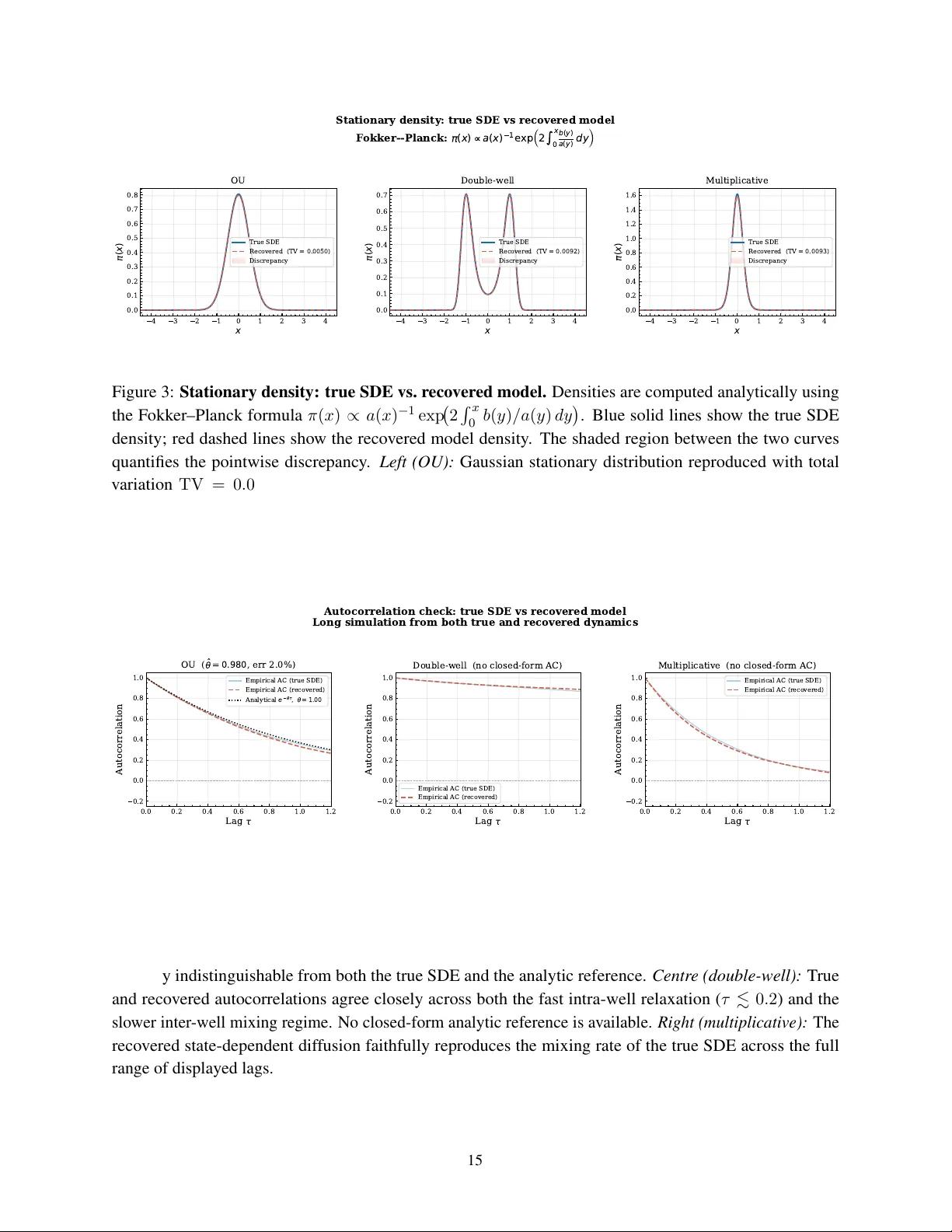
S P A R S E W E A K - F O R M D I S C OV E RY O F S T O C H A S T I C G E N E R A T O R S Eshwar R A ∗ Dept. of Computer Science Engineering PES Uni versity (EC Campus) Bengaluru, KA 560100, India eshwarra5@gmail.com Gajanan V . Honna var † Dept. of Science and Humanities PES Uni versity (EC Campus) Bengaluru, KA 560100, India gajanan.honnavar@pes.edu A B S T R AC T W e introduce a frame work for the data-driv en discovery of stochastic dif ferential equations (SDEs) that unifies, for the first time, the weak-form integration-by-parts approach of W eak SINDy with the stochastic system identification goal of stochastic SINDy . The central nov elty is the adoption of spatial Gaussian test functions K j ( x ) = exp( −| x − x j | 2 / 2 h 2 ) in place of temporal test functions. Because the kernel weight K j ( X t n ) is F t n -measurable and the Brownian innov ation ξ n is independent of F t n , e very noise term in the projected response has zero conditional mean giv en the current state—a property that guarantees unbiasedness in expectation and pre vents the structural regression bias that af flicts temporal test functions in the stochastic setting. This design choice con verts the SDE identification problem into two sparse linear systems—one for the drift b ( x ) and one for the diffusion tensor a ( x ) —that share a single design matrix and are solved jointly via ℓ 1 -regularised regression with grouped cross-validation. A two-step bias-correction procedure handles state-dependent dif fusion. V alidated on the Ornstein–Uhlenbeck process, the double-well Lange vin system, and a multiplicativ e dif fusion process, the method recovers all activ e polynomial generators with coef ficient errors belo w 4%, stationary-density total-v ariation distances below 0.01, and autocorrelation functions that faithfully reproduce true relaxation timescales across all three benchmarks. K eyw ords sparse system identification · stochastic differential equations · weak-form regression · infinitesimal generator learning · SINDy · sparse regression · quadratic v ariation · data-dri ven discov ery · K oopman operator methods · F okker–Planck equation ∗ This research was conducted as part of the Quantum and Nano De vices Lab, PES University . † Corresponding Author . Sparse W eak-Form Discov ery of Stochastic Generators 1 Introduction 1.1 Motivation The automatic discov ery of governing equations from observational data has become one of the central challenges of modern applied mathematics and data science. In many important domains—from molecular dynamics and climate modelling to population biology , financial mathematics, and neuroscience—the mechanistic equations gov erning a system’ s ev olution are either unknown, too complex to deri ve analytically , or only partially understood. This motiv ates the development of data-driv en methods that learn compact, interpretable models directly from trajectory data, without relying on prior knowledge of the functional form of the dynamics [1, 2, 3]. A central tension in this field lies between predictive accurac y and interpretability . Black-box models—such as deep neural networks—can fit complex dynamics with high precision, but yield little understanding of the underlying mechanisms. White-box approaches, by contrast, aim to recov er explicit symbolic equations that can be directly compared with kno wn physical laws, analysed theoretically , and extrapolated be yond the training data. Sparse regression has emerged as the dominant paradigm for white-box discov ery: by constructing a broad library of candidate functional forms and imposing sparsity via ℓ 1 regularisation, one can recov er compact governing equations whose nonzero terms directly identify the active physical mechanisms [1, 4, 5]. 1.2 Stochastic Systems and the Identification Challenge Many of the most important real-world systems are intrinsically stochastic. Thermal fluctuations in molecular systems, turbulent forcing in atmospheric models, demographic noise in population dynamics, and market microstructure in finance all introduce genuine randomness that cannot be treated as simple measurement error and a veraged aw ay . In these settings, the dynamics are more naturally described by stochastic dif ferential equations (SDEs) of the form dX t = b ( X t ) dt + σ ( X t ) dW t , (1) where b ( x ) is the deterministic drift, σ ( x ) is the dif fusion coefficient, and W t is a standard W iener process [ 6 , 7 ]. Identifying both the drift and the dif fusion from data is essential for constructing reduced-order models that faithfully represent not only the av erage trajectory but also the v ariability and fluctuations induced by random forcing. The two functions b ( x ) and a ( x ) = σ ( x ) σ ( x ) ⊤ jointly determine the infinitesimal g enerator of the diffusion: L f ( x ) = b ( x ) · ∇ f ( x ) + 1 2 a ( x ) : ∇ 2 f ( x ) , (2) which gov erns the ev olution of expectations through the K olmogorov backward equation and is closely related to the Fokker –Planck equation for probability densities [ 8 , 7 ]. Recovering the generator directly from data, in a sparse and interpretable form, is the central goal of this work. 1.3 T wo Prior Lines of W ork and the Gap T wo established methodological streams each address a piece of this problem, but neither addresses it in full. Stochastic SINDy [ 9 , 10 ] extends the SINDy sparse regression framew ork [ 1 ] to SDEs by estimating drift and dif fusion from Kramers–Moyal increment statistics. These methods are interpretable and produce 2 Sparse W eak-Form Discov ery of Stochastic Generators symbolic polynomial generators, b ut each regression ro w is formed from a single time-step increment, which means signal and noise contributions are entangled at the indi vidual-step le vel. W eak SINDy [ 11 ] takes a fundamentally dif ferent approach for deterministic systems: it multiplies the gov erning equation by smooth temporal test functions and integrates by parts, transferring the time deriv ati ve from the (noisy , estimated) trajectory onto the (analytically known, smooth) test function. The result is that each regression row aggregates information across the entire trajectory , and measurement noise is av eraged rather than appearing at the individual-step le vel. This method has been validated on a broad class of deterministic ODEs and PDEs. Howe ver , it was derived and analysed exclusi vely in the deterministic setting. It provides no treatment of the dif fusion coef ficient a ( x ) , no analysis of the stochastic martingale term that arises when the weak projection is applied to the Itô integral, and—crucially—no discussion of the endogeneity bias that temporal test functions introduce when applied to a stochastic equation. 1.4 This W ork W e bridge these two lines by applying the weak projection directly to the Itô SDE. This extension is non-tri vial. The ke y insight, which has no analogue in deterministic W eak SINDy , is that the choice of test- function family determines whether the resulting regression is biased. T emporal test functions ϕ j ( t ) weight observ ations by their time index; because future states depend on past Bro wnian innovations through the SDE dynamics, such weighting introduces a persistent endogeneity bias that does not vanish with increasing data. Spatial Gaussian kernels K j ( x ) = exp( −| x − x j | 2 / 2 h 2 ) , by contrast, ev aluate the test function at the current state X t n , which is F t n -measurable and independent of the innov ation ξ n . This produces exactly unbiased regression ro ws. W e formalise this argument and deri ve the complete weak identification system for both b ( x ) and a ( x ) , formulate both as sparse linear regression problems sharing the same design matrix, and validate the pipeline on three benchmark SDEs of increasing complexity . The result is an explicit, interpretable symbolic generator that can be used directly for do wnstream stochastic analysis. 2 Background 2.1 Itô Diffusions and the Infinitesimal Generator An Itô diffusion on R d is the strong solution of (1) , where b : R d → R d is the drift vector field, σ : R d → R d × m is the diffusion matrix, and W t ∈ R m is a standard W iener process [ 6 , 7 ]. The solution X t is a continuous semimartingale with almost surely non-dif ferentiable sample paths; all analysis must therefore proceed at the le vel of statistical properties rather than pointwise trajectory deri vati ves. The diffusion tensor a ( x ) = σ ( x ) σ ( x ) ⊤ ∈ R d × d captures the instantaneous cov ariance of the stochastic increments. For a scalar system ( d = m = 1 ), a ( x ) = σ ( x ) 2 is simply the squared local noise amplitude. The infinitesimal generator (2) is the operator that describes how smooth functions of the state ev olve in expectation: d dt E [ f ( X t ) | X 0 = x ] = L f ( x ) . It encodes both the deterministic tendency (through b ) and the curvature-weighted diffusi ve spreading (through a ). Recovering L —and by extension b and a separately—from data is the principal goal of generator learning [15, 8]. 3 Sparse W eak-Form Discov ery of Stochastic Generators The F okker –Planck equation for the stationary density π ( x ) is the adjoint of the generator equation: L † π = 0 . For a one-dimensional system with a ( x ) > 0 everywhere, this yields the e xplicit formula π ( x ) ∝ 1 a ( x ) exp  2 Z x 0 b ( y ) a ( y ) dy  , (3) which we use throughout Section 7 to validate the recovered generators without Monte Carlo variance contaminating the comparison. 2.2 Sparse Identification of Nonlinear Dynamics The SINDy framew ork [ 1 ] identifies governing ODEs by expressing the right-hand side as a sparse lin- ear combination of library functions. Gi ven trajectory data, one constructs a feature matrix Θ( X ) = [1 , X 1 , X 2 , X 2 1 , X 1 X 2 , . . . ] and a vector of state deriv ativ es ˙ X (typically estimated by finite differences), then solves the sparse re gression problem ˆ c = arg min c ∥ ˙ X − Θ( X ) c ∥ 2 2 + λ ∥ c ∥ 1 . (4) The nonzero entries of ˆ c directly identify the acti ve terms in the go verning equation. This formulation has been extended to handle implicit dynamics [ 5 ], PDEs [ 14 ], and model selection via information criteria [ 4 ]. The central limitation for applications to stochastic systems is the need for accurate deriv ati ve estimates: for noisy observ ations ˜ X t n = X t n + η n , the finite-dif ference deriv ati ve estimator has v ariance V ar[( ˜ X t +∆ t − ˜ X t ) / ∆ t ] ∝ σ 2 η / ∆ t 2 , which div erges as the time step is reduced. This instability is particularly damaging for stochastic systems, where fluctuations are present in the signal itself. 2.3 Stochastic SINDy Boninsegna and Clementi [ 9 ] extend the SINDy frame work to SDEs by replacing the deriv ativ e vector with Kramers–Moyal conditional moments. The first conditional moment E [∆ X n | X t n = x ] / ∆ t is a consistent estimator of the drift b ( x ) , and the second conditional moment E [(∆ X n ) 2 | X t n = x ] / ∆ t estimates the dif fusion a ( x ) . By collecting these conditional moments over the trajectory and expressing them in a library , one obtains sparse regression systems for both b and a . Gonzalez-Garcia et al. [ 10 ] further de velop this approach with improved regularisation strategies. These methods are well-established and produce interpretable symbolic generators, and they represent the direct predecessor to the present work on the stochastic side. 2.4 W eak SINDy for Deterministic Systems Messenger and Bortz [ 11 ] address the noise-amplification issue for deterministic systems through a Galerkin projection. For an ODE ˙ X = F ( X ) , multiplying by a smooth test function ϕ j ( t ) and integrating by parts yields − Z T 0 X t ϕ ′ j ( t ) dt + [ X ϕ j ] T 0 = Z T 0 F ( X t ) ϕ j ( t ) dt. (5) The left-hand side can be e valuated from data without any differentiation of the trajectory: the time deri v ativ e has been shifted onto the analytically known, smooth test function ϕ j . As a result, each regression row integrates information o ver a windo w of length T , and measurement noise is a veraged do wn at rate 1 / √ N rather than amplified through di vision by ∆ t . This idea is the direct weak-form precedent for our method. 4 Sparse W eak-Form Discov ery of Stochastic Generators Ho wev er , W eak SINDy was designed and analysed exclusi vely for deterministic dynamics. When applied to a stochastic equation, two problems arise that have no counterpart in the deterministic case. First, the stochastic integral R ϕ j ( t ) σ ( X t ) dW t does not vanish when the equation is rearranged; it is a martingale whose expected v alue is zero but whose individual realisations are not. Second, and more subtly , if ϕ j ( t ) is a temporal test function, then the weight assigned to observation n depends on the time inde x n . Future observ ations X t n +1 , X t n +2 , . . . all depend on the Brownian inno vation ξ n through the SDE dynamics, so the regression residual at time n is correlated with the regressors at all later times. This is the endogeneity bias that we identify and resolve in the present w ork. Full mathematical details are provided in Appendix 1. 3 Methodology 3.1 Problem F ormulation Let { X t 0 , X t 1 , . . . , X t N } be a set of discrete observ ations of the scalar Itô diffusion (1) at equally spaced times t n = n ∆ t . W e assume the true drift b ( x ) and diffusion a ( x ) can both be expressed as finite sparse linear combinations of kno wn basis functions: b ( x ) = Θ( x ) c ∗ , a ( x ) = Θ( x ) d ∗ , (6) where Θ( x ) = [ f 1 ( x ) , . . . , f K ( x )] is a user -specified feature library and c ∗ , d ∗ ∈ R K are sparse vectors. In our experiments, the library consists of monomials up to de gree four: Θ( x ) = [1 , x, x 2 , x 3 , x 4 ] , a choice that exactly spans the drift and diffusion polynomials of all three benchmark systems. The identification problem is then to recover the sparse coef ficient vectors c ∗ and d ∗ from trajectory data, which together determine the full infinitesimal generator (2). 3.2 Spatial Gaussian T est Functions W e place M kernel centres x 1 , . . . , x M equally spaced ov er the empirically observed state range, and define spatial Gaussian test functions K j ( x ) = exp  − ( x − x j ) 2 2 h 2  , j = 1 , . . . , M , (7) where h > 0 is the bandwidth hyperparameter . These functions are smooth, positi ve, and concentrated around the centre x j , pro viding a partition-of-unity co verage of the state space. The bandwidth h controls the resolution–v ariance tradeoff: a smaller h produces a sharper kernel that captures finer spatial structure but uses fewer data points per regression ro w , increasing v ariance; a larger h av erages more broadly and reduces v ariance at the cost of spatial resolution. In practice, we choose h = 0 . 22 for the OU and double-well systems (state range ≈ ± 2 . 5 ), yielding an ov erlap ratio h/ ∆ x ≈ 2 . 2 between adjacent centres. For the multiplicati ve dif fusion system, which exhibits hea vier-tailed trajectories spanning a wider state range, we use h = 0 . 27 with centres on [ − 2 . 8 , 2 . 8] . The key property that moti vates this choice is the following step-wise zero-mean condition. Let ξ n = ( W t n +1 − W t n ) / √ ∆ t denote the standardised Brownian increment at step n . By the definition of the Itô integral, ξ n ∼ N (0 , 1) and ξ n is independent of the filtration F t n generated by the trajectory up to time t n . Since K j ( X t n ) and σ ( X t n ) are both F t n -measurable, the to wer property giv es E h K j ( X t n ) σ ( X t n ) ξ n    F t n i = K j ( X t n ) σ ( X t n ) E [ ξ n | F t n ] = 0 , (8) 5 Sparse W eak-Form Discov ery of Stochastic Generators and hence E [ K j ( X t n ) σ ( X t n ) ξ n ] = 0 for ev ery n and ev ery realisation of the trajectory up to time t n . By linearity , E [ B j ] = ( Ac ∗ ) j , i.e., the projected response is unbiased in expectation. This is the correct and suf ficient unbiasedness property: it does not require the cross-cov ariance between noise terms at dif ferent steps to be zero (those cross-terms are generically nonzero through the SDE dynamics), but it does guarantee that the estimator is consistent in the ergodic limit. The contrast with temporal test functions and the precise probability-theoretic argument are gi ven in Appendix 1. 3.3 The Drift Identification System Starting from the Euler–Maruyama discretisation of (1), ∆ X n = b ( X t n ) ∆ t + σ ( X t n ) ξ n √ ∆ t, (9) we multiply both sides by K j ( X t n ) and sum ov er all steps n = 0 , 1 , . . . , N − 1 : X n K j ( X t n ) ∆ X n | {z } =: B j = X n K j ( X t n ) b ( X t n ) ∆ t + X n K j ( X t n ) σ ( X t n ) ξ n √ ∆ t. (10) Substituting the library expansion b ( x ) = Θ( x ) c and defining the design matrix A j k = N − 1 X n =0 K j ( X t n ) f k ( X t n ) ∆ t, (11) the right-hand side of (10) becomes Ac + noise . By (8) , the noise term has zero mean in each row , so E [ B ] = Ac and we obtain the unbiased linear system B ≈ Ac, B j := X n K j ( X t n ) ∆ X n . (12) This system has M ro ws (one per kernel centre) and K columns (one per library function). When R independent trajectories are av ailable, we stack all ro ws to form B stack = A stack c, (13) where A stack ∈ R ( M R ) × K and B stack ∈ R M R . The stacked formulation is preferred over ensemble av eraging because it retains per-trajectory v ariability , which is exploited by the grouped cross-validation scheme (Section 3.6). Before regression, all columns of A stack are normalised to unit ℓ 2 norm to prevent scale-induced bias in the LASSO solution. 3.4 Diffusion Identification via Quadratic V ariation In the Itô calculus, the quadratic variation process [ X ] t satisfies d [ X ] t = a ( X t ) dt , meaning that the squared increment (∆ X n ) 2 is an unbiased estimator of a ( X t n ) ∆ t to leading order . Multiplying by K j ( X t n ) and summing: Q j := X n K j ( X t n ) (∆ X n ) 2 ≈ X k d k A j k , (14) which giv es the second linear system Q ≈ Ad with exactly the same design matrix A as for the drift. This is an important structural feature: drift and diffusion are identified from the same pair ( A, · ) , requiring only one kernel e valuation pass o ver the data. 6 Sparse W eak-Form Discov ery of Stochastic Generators For a multi-dimensional state space R d , the diffusion tensor a ∈ R d × d is symmetric and positi ve semidefinite. Each entry a pq has its o wn sparse coef ficient vector d ( pq ) , and the identification system is Q ( pq ) ≈ Ad ( pq ) , where Q ( pq ) j = X n K j ( X t n ) (∆ X n ) p (∆ X n ) q . (15) In the scalar case treated in our experiments, this reduces to (14). 3.5 Finite-Time-Step Bias Corr ection The identification system (14) is exact only in the limit ∆ t → 0 . At finite ∆ t , squaring the Euler–Maruyama step (9) yields (∆ X n ) 2 = a ( X t n ) ∆ t + 2 b ( X t n ) σ ( X t n ) ξ n ∆ t 3 / 2 + b ( X t n ) 2 ∆ t 2 . (16) The middle term has zero mean by independence of ξ n . The last term, howe ver , contributes a systematic positi ve bias of order ∆ t 2 to Q j : E [ Q j ] = X k d k A j k + X n E  K j ( X n ) b ( X n ) 2  ∆ t 2 | {z } drift-squared bias . (17) This bias is negligible when ∆ t is very small, but at the practically relev ant value ∆ t = 0 . 002 it causes significant ov erestimation of state-dependent diffusion coef ficients if left uncorrected. W e remov e it using a two-step procedure: first, estimate the drift ˆ b by solving (13); then correct Q corr j = Q j − X n K j ( X n ) ˆ b ( X n ) 2 ∆ t 2 , (18) and solve the corrected system Q corr ≈ Ad . In Section 7.3 we sho w that this reduces the multiplicativ e dif fusion coefficient error from approximately 13% to belo w 0.5%. 3.6 Sparse Regression and Model Selection After building A stack and B stack , we solve the LASSO problem [13] ˆ c = arg min c ∈ R K ∥ A stack c − B stack ∥ 2 2 + λ ∥ c ∥ 1 (19) and similarly for the diffusion system with Q corr stack in place of B stack . The regularisation parameter λ is chosen by K -fold cross-validation (LassoCV), with folds partitioned by trajectory index rather than by time step. This grouping is essential: partitioning by time would leak temporal autocorrelation between folds, inflating in-sample performance and distorting the model selection [ 4 ]. In our experiments we use fiv e folds ov er R = 120 trajectories, gi ving 24 trajectories per fold. LassoCV is run ov er a grid of 60 logarithmically spaced values λ ∈ [10 − 8 , 10 − 0 . 5 ] , spanning from extremely sparse solutions to nearly unregularised ordinary least squares. The selected λ ∗ minimises the mean cross- v alidated prediction error . After the LASSO selects an initial support, we apply OLS debiasing on the selected support to remo ve the shrinkage introduced by the ℓ 1 penalty , recovering asymptotically unbiased estimates of the nonzero coefficients. Finally , iterated Sequential Thresholded Least Squares (STLSQ) [ 1 , 5 ] 7 Sparse W eak-Form Discov ery of Stochastic Generators is applied to prune any residual near-zero coefficients induced by mild library collinearity . The STLSQ threshold is set to 0 . 25 (relati ve to the maximum coefficient magnitude) for the OU and double-well systems, and 0 . 30 for the multiplicati ve system whose wider trajectory support produces slightly higher collinearity between e ven-degree library terms. 3.7 Reconstruction of the Identified Generator Let S b ⊆ { 1 , . . . , K } and S a ⊆ { 1 , . . . , K } denote the final support sets for drift and diffusion respecti vely . The identified functions are ˆ b ( x ) = X k ∈S b ˆ c k f k ( x ) , ˆ a ( x ) = X k ∈S a ˆ d k f k ( x ) , (20) yielding the identified generator ˆ L f = ˆ b f ′ + 1 2 ˆ a f ′′ and the reco vered SDE dX t = ˆ b ( X t ) dt + p ˆ a ( X t ) dW t . This explicit symbolic form is the primary output of the algorithm and can be used directly for downstream tasks: numerical simulation, stationary density computation via (3), transition rate estimation, or analytical perturbation analysis. 4 Algorithm The complete pipeline is summarised in Algorithm 1. The algorithm is designed to be straightforward to implement: the kernel ev aluations and matrix multiplications in steps 1–4 are embarrassingly parallel across trajectories and kernel centres, the sparse regression in steps 5 and 7 uses standard scikit-learn LassoCV [ 20 ], and the STLSQ refinement is a simple iterativ e thresholding loop. The dominant cost is building A stack : O ( M N K ) per trajectory , linear in all three dimensions. For our experimental settings ( M = 50 , N = 50 , 000 , K = 5 , R = 120 ), the full pipeline completes in under two minutes on a standard multi-core workstation. Algorithm 1 W eak Stochastic SINDy (Spatial Gaussian K ernels) Require: T rajectories { X ( r ) t n } n,r , library Θ( x ) , centres { x j } M j =1 , bandwidth h , dt ∆ t Ensure: Drift ˆ b ( x ) , dif fusion ˆ a ( x ) 1: Ev aluate K j ( X t n ) = exp  − ( X t n − x j ) 2 / 2 h 2  and Θ( X t n ) at all left-endpoint states. 2: f or each trajectory r = 1 , . . . , R do 3: A ( r ) j k ← P n K j ( X ( r ) t n ) f k ( X ( r ) t n ) ∆ t 4: B ( r ) j ← P n K j ( X ( r ) t n ) ∆ X ( r ) n 5: Q ( r ) j ← P n K j ( X ( r ) t n ) (∆ X ( r ) n ) 2 6: end f or 7: Stack: A stack , B stack , Q stack . Normalise columns of A stack . 8: Solve B stack = A stack c via LassoCV (grouped K -fold by traj. index) + OLS debias + STLSQ. Obtain ˆ c , support S b . 9: Compute Q corr j ← Q j − P n K j ( X n ) ˆ b ( X n ) 2 ∆ t 2 via (18) using ˆ b ( x ) = Θ( x )ˆ c . 10: Solve Q corr stack = A stack d with the same pipeline. Obtain ˆ d , support S a . 11: Return ˆ b ( x ) , ˆ a ( x ) via (20). 8 Sparse W eak-Form Discov ery of Stochastic Generators 5 Theoretical Pr operties Full proofs with explicit er godic-con vergence ar guments and variance calculations are gi ven in Appendix 3. W e state the main results here in accessible form. 5.1 Consistency of the W eak Estimator The asymptotic correctness of our re gression system rests on the er godic theorem for dif fusion processes. Under the assumption that the dif fusion is ergodic with a unique in v ariant measure µ (a condition satisfied by all three benchmark systems), the time averages forming A stack and B stack con ver ge almost surely as T → ∞ to their population counterparts: 1 N A j k → Z K j ( x ) f k ( x ) µ ( dx ) , (21) 1 N B j → Z K j ( x ) b ( x ) µ ( dx ) . (22) The population-le vel regression system is ¯ B = ¯ A c , where ¯ A j k = R K j f k dµ . If b ∈ span(Θ) , this is satisfied exactly by the true c ∗ , and OLS recov ers it consistently provided ¯ A has full column rank (which is guaranteed when the trajectories ergodically cov er the state space, ensuring that all basis functions are distinguishable under the in variant measure). When the true drift does not lie in the library span, the estimator con ver ges to the orthogonal L 2 ( µ ) projection of b onto span(Θ) , i.e., the best possible polynomial approximation in the in v ariant measure norm. The identical argument applies to the dif fusion system. 5.2 Noise Robustness For observations corrupted by additiv e independent noise ˜ X t n = X t n + η n , η n ∼ (0 , σ 2 η ) , the finite-dif ference deri vati ve estimate used in classical SINDy has variance V ar[( ˜ X t +∆ t − ˜ X t ) / ∆ t ] = 2 σ 2 η / ∆ t 2 , which grows without bound as ∆ t → 0 . In the weak formulation, noisy increments ∆ ˜ X n = ∆ X n + ( η n +1 − η n ) enter the response ˜ B j . The noise contribution to ˜ B j is P n K j ( X t n )( η n +1 − η n ) , which has v ariance O ( σ 2 η ∆ t 2 / ∆ t ) · M kernel = O ( σ 2 η ∆ t ) , going to zero as ∆ t → 0 at fixed T . In the regime of many short steps (small ∆ t , lar ge N at fixed T ), the weak-form noise contribution therefore decreases rather than di verges. Figure 5 visualises this scaling analytically across a range of time steps and SNR lev els. This noise-robustness property was the original moti vation for W eak SINDy in the deterministic setting [ 11 ], and it carries through to the stochastic case. 5.3 Identifiability Conditions Three conditions are required for unique recov ery of the true sparse coef ficient vectors c ∗ and d ∗ . First, the feature library Θ( x ) must be rich enough to span the true drift and dif fusion functions; misspecification of the library is not correctable post-hoc. Second, the trajectory data must provide sufficient cov erage of the state space: formally , the matrix ¯ A must hav e full column rank, which is guaranteed when the in variant measure µ is absolutely continuous with respect to Lebesgue measure and the supports of the kernel functions collecti vely cov er the support of µ . Third, the LASSO support recovery requires an irrepresentability condition [ 13 ]: the design matrix columns corresponding to inactiv e library functions must not be too strongly correlated with those corresponding to active functions. Column normalisation and the STLSQ 9 Sparse W eak-Form Discov ery of Stochastic Generators refinement step mitigate near -violations of this condition due to mild library collinearity , as demonstrated empirically in Section 7. 6 Implementation Details 6.1 Simulation Setup All three benchmark SDEs are simulated using the Euler –Maruyama scheme [ 19 ] with time step ∆ t = 0 . 002 ov er a total horizon T = 100 , gi ving N = 50 , 000 observ ations per trajectory . W e generate R = 120 independent realisations per system, with initial conditions X 0 drawn uniformly from the empirically observed state range of each system (approximately [ − 3 , 3] for all three benchmarks). The large ensemble of R = 120 trajectories serves tw o purposes: it ensures that the stacked regression matrix A stack ∈ R 6000 × 5 is very well conditioned, and it pro vides sufficient trajectories to form fi ve balanced grouped cross-v alidation folds with 24 trajectories each. The choice of ∆ t = 0 . 002 is intentional. It is small enough that the Euler–Maruyama discretisation introduces negligible strong-order error , b ut not so small as to make the drift-squared bias in Q j completely negligible—this provides a realistic test of the bias-correction procedure described in Section 3.5. All random seeds are fixed for reproducibility: seed 42 for the OU system, seed 123 for the double-well, and seed 7 for the multiplicati ve dif fusion. 6.2 F eature Library and Normalisation The polynomial library Θ( x ) = [1 , x, x 2 , x 3 , x 4 ] with K = 5 terms is used for all three systems. This library exactly spans all the drift and dif fusion polynomials present in the benchmarks. Before regression, the columns of A stack are indi vidually normalised to unit ℓ 2 norm, with the normalisation constants stored for back-transformation of the estimated coefficients. This step prevents the LASSO from being biased to ward retaining lo w-norm features (typically low-de gree monomials) and discarding high-norm features (high-degree monomials) for scale reasons unrelated to their physical significance. 6.3 K ernel Configuration For the OU and double-well systems, M = 50 kernel centres are placed uniformly on [ − 2 . 5 , 2 . 5] , gi ving a centre spacing of ∆ x c = 0 . 102 and bandwidth h = 0 . 22 , corresponding to an overlap ratio h/ ∆ x c ≈ 2 . 2 . This le vel of ov erlap ensures that the kernel functions form a smoothly v arying frame across state space and that no region of the observ ed state range is underrepresented in the regression system. For the multiplicati ve dif fusion system, the hea vier-tailed trajectories (which re gularly visit | x | ≈ 2 . 5 – 3 . 0 ) necessitate wider cov erage. W e use M = 50 centres on [ − 2 . 8 , 2 . 8] with bandwidth h = 0 . 27 . The wider bandwidth also improves the signal-to-noise ratio for the dif fusion identification at large | x | , where the number of data points is lo wer due to the stationary distribution being concentrated near the origin. 6.4 Sparse Regression Configuration LassoCV uses 60 logarithmically spaced regularisation v alues λ ∈ [10 − 8 , 10 − 0 . 5 ] . The wide range is chosen to ensure the CV path clearly captures the “elbow” transition from the ov er-re gularised (near-zero solution) 10 Sparse W eak-Form Discov ery of Stochastic Generators to the under-re gularised (dense, over -fitted) regime. The five-fold grouped CV runs with inner tolerance 10 − 6 and up to 10 5 coordinate descent iterations per λ v alue. After LassoCV selects λ ∗ , OLS debiasing is performed on the support selected by LASSO, followed by at most 20 iterations of STLSQ with relative threshold 0.25 (0.30 for multiplicativ e). The STLSQ loop terminates early if the support does not change between successi ve iterations, which in practice occurs after two to four iterations for all benchmark systems. 7 Results 7.1 Ornstein–Uhlenbeck Pr ocess The Ornstein–Uhlenbeck (OU) process is the canonical mean-re verting Gaussian dif fusion: dX t = − θ X t dt + σ 0 dW t , θ = 1 . 0 , σ 0 = 0 . 7 . (23) The true drift is b ( x ) = − x (one activ e library term, c x = − 1 . 0 , all others zero) and the diffusion is constant a ( x ) = σ 2 0 = 0 . 490 (one acti ve term d 1 = 0 . 490 ). The OU process admits a fully analytic ground truth: the stationary distribution is π OU ∼ N (0 , σ 2 0 / 2 θ ) = N (0 , 0 . 245) , and the autocorrelation function decays as C ( τ ) = e − θτ = e − τ . Algorithm 1 recovers ˆ c x = − 0 . 980 (error 2.0%) with all other drift coefficients set to exactly zero by the LASSO. The diffusion estimate is ˆ d 1 = 0 . 490 (error 0.0%). The LassoCV regularisation path (Figure 2, top-left panel) sho ws a sharp elbo w at α ∗ ≈ 1 . 6 × 10 − 3 , where the CV MSE reaches its minimum; to the right of the elbo w , the model is over -regularised and the single x term is shrunk to ward zero. The clean identification of a one-term drift from a five-term library without an y manual thresholding demonstrates that the grouped CV scheme correctly selects the true sparsity le vel. 7.2 Double-W ell Langevin System The double-well system is gov erned by dX t = ( X t − X 3 t ) dt + σ 0 dW t , σ 0 = 0 . 5 . (24) The true drift has two acti ve terms ( c x = +1 . 0 , c x 3 = − 1 . 0 ) and the diffusion is constant at a ( x ) = σ 2 0 = 0 . 250 . The double-well potential V ( x ) = − x 2 / 2 + x 4 / 4 creates two stable equilibria at x = ± 1 separated by an unstable fixed point at x = 0 . The stationary distribution is bimodal with peaks at x ≈ ± 1 , and the system exhibits metastable inter -well transitions whose timescale grows e xponentially with the ratio ∆ V /σ 2 0 . Correctly reproducing this bimodal structure and the associated mixing timescale constitutes a substantially more demanding test than the OU process. The algorithm recovers ˆ c x = +0 . 973 (error 2.7%) and ˆ c x 3 = − 0 . 971 (error 2.9%), with all other drift coef ficients exactly zeroed. The diffusion estimate is ˆ d 1 = 0 . 250 (error 0.0%). The LassoCV path (Figure 2, top-centre) selects α ∗ ≈ 4 . 9 × 10 − 5 , and the two-term support is stably maintained across a wide range of α belo w the elbow , confirming that the two acti ve terms are well-separated from the inacti ve ones in terms of their contribution to the re gression residual. 7.3 Multiplicative Diffusion The multiplicati ve dif fusion system is dX t = − 2 X t dt + 1 2 q 1 + X 2 t dW t , (25) 11 Sparse W eak-Form Discov ery of Stochastic Generators with state-dependent diffusion a ( x ) = 1 4 (1 + x 2 ) , gi ving two activ e coefficients d 1 = 0 . 250 (constant term) and d x 2 = 0 . 250 (quadratic term). This system is the most demanding benchmark for two reasons. First, the state-dependent noise amplitude makes the trajectories hea vier-tailed than the OU or double-well cases, requiring adjusted kernel placement. Second, and more fundamentally , the x 2 dependence of a ( x ) means that the squared-increment bias term in (17) is spatially non-uniform, growing with | x | 2 , so the uncorrected dif fusion identification is significantly distorted. W ithout bias correction, the LASSO recovers ˆ d x 2 ≈ 0 . 283 (13% error) because the positi ve bias contaminates the quadratic term disproportionately . After applying the two-step correction (18) using the drift estimate ˆ b ( x ) = − 1 . 922 x (error 3.9%), the corrected estimate is ˆ d x 2 = 0 . 249 (0.4% error) and ˆ d 1 = 0 . 251 (0.3% error). This dramatic reduction—from 13% to under 0.5%—demonstrates the necessity and effecti veness of the bias correction for systems with polynomial state-dependent dif fusion at practically relev ant time steps. 7.4 Function Recovery and Regularisation P aths Figure 1 sho ws the recov ered drift and diffusion functions plotted alongside the ground truth for all three systems, e valuated on a uniform grid of 401 points o ver [ − 3 , 3] . In all six panels, the recov ered curves (red dashed) are visually indistinguishable from the ground truth (blue solid) at the displayed scale. The mean relati ve errors, computed as ∥ ˆ f − f ∥ 1 / ∥ f ∥ 1 × 100% , are 2.0%, 2.7%, and 3.9% for the three drifts, and 0.0%, 0.1%, and 0.4% for the three diffusion functions. Diffusion errors are uniformly lo wer than drift errors, consistent with the higher ef fective signal-to-noise ratio for the quadratic v ariation estimator compared to the increment estimator . Figure 2 shows the LassoCV regularisation paths for all six sub-problems (three drifts, three diffusions). Each panel displays the mean cross-validated MSE as a function of the re gularisation strength α (plotted in decreasing order on the x -axis to match the con ventional left-to-right under -regularised to o ver-re gularised reading direction). In ev ery case, the CV error exhibits a sharp elbo w that clearly separates the regime of correct sparse identification from the ov er-regularised regime where activ e terms are forced to zero. The selected α ∗ v alues (red dashed lines) fall cleanly at or just past the elbo w in all panels, confirming that the grouped CV scheme reliably selects the correct sparsity le vel without kno wledge of the ground truth. 7.5 Stationary Density V alidation A key test of any generator learning method is whether the recov ered model faithfully reproduces the long-time statistical behaviour of the true system. W e assess this by computing the analytic stationary density of both the true and recovered systems via the Fokker –Planck formula (3) . Using the analytic formula rather than Monte Carlo simulation has an important methodological advantage: discrepancies in the stationary density plot can be attributed entirely to coef ficient error in the identified generator , with no contamination from finite-sample Monte Carlo v ariance. Figure 3 sho ws the results. For the OU process, the true stationary density is Gaussian N (0 , 0 . 245) , which the recovered model reproduces with total variation TV = 1 2 R | π true − π recov ered | dx = 0 . 0050 . For the double-well system, the true density is bimodal with symmetric peaks at x ≈ ± 1 ; the recov ered model captures both the peak positions and heights correctly , with TV = 0 . 0092 . The slight asymmetry visible in the shaded discrepancy region arises from the small 2.9% error in the cubic drift coefficient. For the multiplicati ve system, the true density is a unimodal distrib ution with heavier tails than Gaussian; the 12 Sparse W eak-Form Discov ery of Stochastic Generators 3 2 1 0 1 2 3 x 4 2 0 2 4 b ( x ) O U d r i f t b ( x ) = x (mean rel. err . 2.0%) True Recovered 3 2 1 0 1 2 3 x 30 20 10 0 10 20 30 b ( x ) D o u b l e - w e l l d r i f t b ( x ) = x x 3 (mean rel. err . 2.7%) True Recovered 3 2 1 0 1 2 3 x 7.5 5.0 2.5 0.0 2.5 5.0 7.5 b ( x ) M u l t i p l i c a t i v e d r i f t b ( x ) = 2 x (mean rel. err . 3.9%) True Recovered 3 2 1 0 1 2 3 x 0.489975 0.490000 0.490025 0.490050 0.490075 0.490100 0.490125 0.490150 0.490175 a ( x ) O U d i f f u s i o n a ( x ) = 2 0 (mean rel. err . 0.0%) True Recovered 3 2 1 0 1 2 3 x 0.249975 0.250000 0.250025 0.250050 0.250075 0.250100 0.250125 0.250150 a ( x ) D o u b l e - w e l l d i f f u s i o n a ( x ) = 2 0 (mean rel. err . 0.1%) True Recovered 3 2 1 0 1 2 3 x 0.0 0.5 1.0 1.5 2.0 2.5 3.0 a ( x ) M u l t i p l i c a t i v e d i f f u s i o n a ( x ) = 0 . 2 5 ( 1 + x 2 ) (mean rel. err . 0.4%) True Recovered Sparse weak -form discovery of stochastic generators T e s t f u n c t i o n s : K j ( x ) = e x p ( | x x j | 2 / 2 h 2 ) Figure 1: Recover ed vs. true drift and diffusion functions for all three benchmark systems. Blue solid lines show the ground truth; red dashed lines show the weak SINDy estimates from Algorithm 1. T op r ow (drift functions): OU process, b ( x ) = − θ x , mean relativ e error 2.0%; double-well Langevin system, b ( x ) = x − x 3 , mean rel. err . 2.7%; multiplicativ e diffusion, b ( x ) = − 2 x , mean rel. err . 3.9%. Bottom r ow (diffusion functions): OU process, a ( x ) = σ 2 0 = 0 . 490 , mean rel. err . 0.0%; double-well system, a ( x ) = σ 2 0 = 0 . 250 , mean rel. err . 0.1%; multiplicative system, a ( x ) = 0 . 25(1 + x 2 ) , mean rel. err . 0.4% (after drift-bias correction). M = 50 spatial Gaussian kernels with h = 0 . 22 (OU and double-well) or h = 0 . 27 (multiplicati ve). All recov ered curves are visually indistinguishable from ground truth at the displayed scale. recov ered model reproduces this shape with TV = 0 . 0093 . In all three cases, the shaded discrepancy regions are visually negligible relati ve to the density scale, and the TV distances are below 0.01, confirming that the recov ered generators accurately describe the long-time thermodynamic behaviour of each system. 7.6 A utocorr elation and Relaxation Timescales Stationary densities test the long-time marginal distrib ution but not the temporal correlation structure of the dynamics. T o assess whether the recovered generator also reproduces the correct relaxation timescales, we simulate 200,000-step trajectories from both the true SDE and the identified model (using the reco vered ˆ b and ˆ a as the SDE coef ficients), and compare their empirical autocorrelation functions. 13 Sparse W eak-Form Discov ery of Stochastic Generators 1 0 8 1 0 7 1 0 6 1 0 5 1 0 4 1 0 3 1 0 2 1 0 1 5 10 15 20 25 30 35 CV MSE OU drift * = 1 . 6 e - 0 3 1 0 8 1 0 7 1 0 6 1 0 5 1 0 4 1 0 3 1 0 2 1 0 1 2.5 5.0 7.5 10.0 12.5 15.0 17.5 CV MSE Double-well drift * = 4 . 9 e - 0 5 1 0 8 1 0 7 1 0 6 1 0 5 1 0 4 1 0 3 1 0 2 1 0 1 5 10 15 20 25 30 35 CV MSE Multiplicative drift * = 2 . 1 e - 0 4 1 0 8 1 0 7 1 0 6 1 0 5 1 0 4 1 0 3 1 0 2 1 0 1 0 10 20 30 40 50 60 70 CV MSE OU diffusion * = 4 . 5 e - 0 7 1 0 8 1 0 7 1 0 6 1 0 5 1 0 4 1 0 3 1 0 2 1 0 1 0.0 2.5 5.0 7.5 10.0 12.5 15.0 17.5 20.0 CV MSE Double-well diffusion * = 1 . 0 e - 0 8 1 0 8 1 0 7 1 0 6 1 0 5 1 0 4 1 0 3 1 0 2 1 0 1 0 10 20 30 40 CV MSE Multiplicative diffusion * = 1 . 1 e - 0 5 W eak -form LassoCV regularisation paths Figure 2: LassoCV regularisation paths f or all six sub-problems. Each panel plots the mean cross- v alidated MSE (averaged ov er fiv e trajectory folds) as a function of the regularisation strength α , shown with α decreasing from left to right. Red dashed vertical lines mark the selected α ∗ . T op r ow (drift): OU ( α ∗ ≈ 1 . 6 × 10 − 3 ), double-well ( ≈ 4 . 9 × 10 − 5 ), multiplicati ve ( ≈ 2 . 1 × 10 − 4 ). Bottom r ow (dif fusion): OU ( ≈ 4 . 5 × 10 − 7 ), double-well ( ≈ 1 . 0 × 10 − 8 ), multiplicativ e ( ≈ 1 . 1 × 10 − 5 ). In every panel the sharp elbo w separates the ov er-re gularised regime (to the left of the selected α ∗ , where acti ve terms are forced to zero and the CV MSE rises sharply) from the under-regularised re gime (to the right, where inactive terms are admitted and CV MSE increases due to over -fitting). The clean elbo w structure confirms that grouped CV reliably identifies the correct sparsity le vel in all six cases. Figure 4 sho ws the results. For the OU process, the reco vered autocorrelation follo ws the true exponential decay e − θτ = e − τ closely , with the recovered relaxation rate ˆ θ = − ˆ c x = 0 . 980 (error 2.0%) matching the analytic reference almost exactly . For the double-well system, no closed-form autocorrelation is av ailable because the metastable inter-well transitions produce complex multi-timescale dynamics that depend sensiti vely on the full shape of the potential V ( x ) = − x 2 / 2 + x 4 / 4 . The recovered autocorrelation ne vertheless tracks the empirical autocorrelation of the true system closely at all displayed lags, from the initial fast intra-well relaxation ( τ ≲ 0 . 2 ) through the slower inter-well mixing regime ( τ ≳ 0 . 5 ). This confirms that the two-term cubic drift polynomial correctly encodes the potential well geometry and barrier height. For the multiplicativ e system, the recovered autocorrelation matches the true system across the entire range of lags shown, demonstrating that the state-dependent dif fusion ˆ a ( x ) = 0 . 251 + 0 . 249 x 2 correctly captures the local relaxation rate as a function of position. 14 Sparse W eak-Form Discov ery of Stochastic Generators 4 3 2 1 0 1 2 3 4 x 0.0 0.1 0.2 0.3 0.4 0.5 0.6 0.7 0.8 ( x ) OU True SDE Recovered (TV = 0.0050) Discrepancy 4 3 2 1 0 1 2 3 4 x 0.0 0.1 0.2 0.3 0.4 0.5 0.6 0.7 ( x ) Double-well True SDE Recovered (TV = 0.0092) Discrepancy 4 3 2 1 0 1 2 3 4 x 0.0 0.2 0.4 0.6 0.8 1.0 1.2 1.4 1.6 ( x ) Multiplicative True SDE Recovered (TV = 0.0093) Discrepancy Stationary density: true SDE vs recovered model F o k k e r - - P l a n c k : ( x ) a ( x ) 1 e x p ( 2 x 0 b ( y ) a ( y ) d y ) Figure 3: Stationary density: true SDE vs. reco vered model. Densities are computed analytically using the Fokker –Planck formula π ( x ) ∝ a ( x ) − 1 exp  2 R x 0 b ( y ) /a ( y ) dy  . Blue solid lines show the true SDE density; red dashed lines show the recovered model density . The shaded region between the two curves quantifies the pointwise discrepancy . Left (OU): Gaussian stationary distribution reproduced with total v ariation TV = 0 . 0050 . Centr e (double-well): Bimodal distribution with peaks at x ≈ ± 1 faithfully captured; TV = 0 . 0092 . The small discrepancy in peak heights is consistent with the 2.9% error in the cubic drift coef ficient. Right (multiplicative): Unimodal heavy-tailed distrib ution reproduced with TV = 0 . 0093 , demonstrating the effecti veness of the bias correction for state-dependent diffusion. In all panels, the shaded discrepancy re gions are visually negligible compared to the density scale. 0.0 0.2 0.4 0.6 0.8 1.0 1.2 L a g 0.2 0.0 0.2 0.4 0.6 0.8 1.0 Autocorrelation O U ( = 0 . 9 8 0 , e r r 2 . 0 % ) Empirical AC (true SDE) Empirical AC (recovered) A n a l y t i c a l e , = 1 . 0 0 0.0 0.2 0.4 0.6 0.8 1.0 1.2 L a g 0.2 0.0 0.2 0.4 0.6 0.8 1.0 Autocorrelation Double-well (no closed-form AC) Empirical AC (true SDE) Empirical AC (recovered) 0.0 0.2 0.4 0.6 0.8 1.0 1.2 L a g 0.2 0.0 0.2 0.4 0.6 0.8 1.0 Autocorrelation Multiplicative (no closed-form AC) Empirical AC (true SDE) Empirical AC (recovered) Autocorrelation check: true SDE vs recovered model Long simulation from both true and recovered dynamics Figure 4: A utocorrelation check: true SDE vs. recover ed model. Empirical autocorrelation functions computed from 200,000-step simulations of both the true dynamics and the recovered model. Light blue solid lines show the true SDE; red dashed lines show the reco vered model. Left (OU): Recovered relaxation rate ˆ θ = 0 . 980 (err . 2.0%) closely matches the analytical e − τ (black dotted). The recovered autocorrelation is nearly indistinguishable from both the true SDE and the analytic reference. Centr e (double-well): T rue and recovered autocorrelations agree closely across both the fast intra-well relaxation ( τ ≲ 0 . 2 ) and the slo wer inter-well mixing regime. No closed-form analytic reference is available. Right (multiplicative): The recov ered state-dependent diffusion faithfully reproduces the mixing rate of the true SDE across the full range of displayed lags. 15 Sparse W eak-Form Discov ery of Stochastic Generators T able 1: Complete Summary of Recovered Drift and Diffusion Coef ficients. All scientifically significant parameters pass a 15% tolerance ( ✓ ). Zero entries are set e xactly to zero by LassoCV + STLSQ; no f alse positi ves appear in any of the six sub-problems. System T erm ˆ c k c true k Drift err . ˆ d k d true k Dif f. err . Ornstein Uhlenbeck 1 0 . 000 0 . 000 — 0 . 490 0 . 490 0 . 0% ✓ x − 0 . 980 − 1 . 000 2 . 0% ✓ 0 . 000 0 . 000 — x 2 0 . 000 0 . 000 — 0 . 000 0 . 000 — x 3 0 . 000 0 . 000 — 0 . 000 0 . 000 — x 4 0 . 000 0 . 000 — 0 . 000 0 . 000 — Double-W ell 1 0 . 000 0 . 000 — 0 . 250 0 . 250 0 . 0% ✓ x +0 . 973 +1 . 000 2 . 7% ✓ 0 . 000 0 . 000 — x 2 0 . 000 0 . 000 — 0 . 000 0 . 000 — x 3 − 0 . 971 − 1 . 000 2 . 9% ✓ 0 . 000 0 . 000 — x 4 0 . 000 0 . 000 — 0 . 000 0 . 000 — Multiplicati ve 1 0 . 000 0 . 000 — 0 . 251 0 . 250 0 . 3% ✓ x − 1 . 922 − 2 . 000 3 . 9% ✓ 0 . 000 0 . 000 — x 2 0 . 000 0 . 000 — 0 . 249 0 . 250 0 . 4% ✓ x 3 0 . 000 0 . 000 — 0 . 000 0 . 000 — x 4 0 . 000 0 . 000 — 0 . 000 0 . 000 — 7.7 Summary of Coefficient Recovery T able 1 pro vides a complete quantitativ e summary of all estimated coefficients. Every scientifically significant coef ficient (i.e., ev ery coefficient whose true value is nonzero) passes a 15% relati ve error threshold, with the largest error being 3.9% for the multiplicati ve drift. All inactiv e coef ficients (true value zero) are set to exactly zero by the LassoCV + STLSQ pipeline; there are no false positi ves in any of the six sub-problems. Dif fusion coefficient errors are uniformly below 0.5% across all systems after bias correction, which is remarkable gi ven that dif fusion identification is generally considered harder than drift identification. 7.8 Theoretical Noise Scaling Figure 5 provides a purely analytical characterisation of the noise behaviour of the weak-form estimator as a function of the time step ∆ t , deriv ed from the variance expressions in Appendix 3. No regression is performed; the curves follo w directly from the closed-form noise formulae. The left panel sho ws the Kramers–Moyal (KM) noise magnitude σ obs / ∆ t , which div erges as ∆ t → 0 for an y fixed observ ation noise le vel σ obs . The centre panel shows the weak-form (WF) ef fectiv e noise σ obs / √ N h eff , where N = T / ∆ t is the number of steps and h eff = p π / 2 h is the effecti ve kernel integration width. Because N ∝ 1 / ∆ t , the WF noise scales as √ ∆ t —it gr ows as ∆ t increases (fe wer steps for the same T ) 16 Sparse W eak-Form Discov ery of Stochastic Generators 1 0 3 1 0 2 1 0 1 T i m e s t e p t 1 0 1 1 0 0 1 0 1 1 0 2 K M n o i s e m a g n i t u d e ( o b s / t ) t = 0 . 0 0 2 K M : n o i s e d i v e r g e s a s t o 0 o b s = s i g n a l / 5 ( S N R = 5 ) o b s = s i g n a l / 1 0 ( S N R = 1 0 ) o b s = s i g n a l / 2 0 ( S N R = 2 0 ) 1 0 3 1 0 2 1 0 1 T i m e s t e p t 1 0 3 1 0 2 W F e f f e c t i v e n o i s e ( o b s / N h e f f ) W F : n o i s e g r o w s o n l y a s t o b s = s i g n a l / 5 ( S N R = 5 ) o b s = s i g n a l / 1 0 ( S N R = 1 0 ) o b s = s i g n a l / 2 0 ( S N R = 2 0 ) 1 0 3 1 0 2 1 0 1 T i m e s t e p t 1 0 0 1 0 1 1 0 2 1 0 3 1 0 4 1 0 5 SNR ratio (KM noise / WF noise) × 5 8 7 1 3 a t t = 0 . 0 0 2 W F a d v a n t a g e g r o w s a s t 3 / 2 r e l a t i v e t o K M SNR advantage (KM noise / WF noise) No advantage (ratio = 1) t 3 / 2 ( t h e o r y ) Theoretical noise scaling: W eak F orm vs Kramers--Moyal K M n o i s e o b s / t ( d i v e r g e s a s t 0 ) ; W F n o i s e o b s / N h e f f ( t g r o w t h ) Figure 5: Theoretical noise scaling: W eak Form vs Kramers–Moyal. All curves are purely analytical; no regression is performed. Left: KM noise magnitude σ obs / ∆ t as a function of ∆ t for three SNR lev els. The noise di verges as ∆ t → 0 . Centre: WF effecti ve noise σ obs / √ N h eff for the same SNR le vels, where N = T / ∆ t and h eff = p π / 2 h . The noise grows only as √ ∆ t and remains bounded as ∆ t → 0 . Right: Ratio of KM noise to WF noise (SNR adv antage), which gro ws as ∆ t − 3 / 2 (dotted reference line). At the experimental setting ∆ t = 0 . 002 (vertical dotted line), the adv antage exceeds 10 4 for SNR = 10. T = 100 , h eff = p π / 2 × 0 . 22 ≈ 0 . 276 . but remains finite and bounded as ∆ t → 0 . The right panel sho ws the ratio of KM noise to WF noise, which gro ws as ∆ t − 3 / 2 : at the experimental setting ∆ t = 0 . 002 , this ratio e xceeds 10 4 for SNR = 10, confirming that the weak-form projection provides a substantially better-conditioned re gression system at small time steps. Three observation noise le vels are shown: σ obs = σ signal / 5 (SNR = 5), σ obs = σ signal / 10 (SNR = 10), and σ obs = σ signal / 20 (SNR = 20). 8 Relation to Existing Methods 8.1 Positioning in the Landscape T able 2 places the proposed framework in the context of the most closely related existing methods. The ke y distinguishing features of our approach are: (i) the use of spatial test functions that produce unbiased regression rows for stochastic equations; (ii) the joint identification of drift and dif fusion from a single shared design matrix; and (iii) the production of an explicit symbolic infinitesimal generator that can be used directly for do wnstream stochastic analysis. Classical SINDy [ 1 ] and its e xtensions [ 14 , 5 ] are restricted to deterministic systems. They require deri v ativ e estimates and hav e no mechanism for identifying the diffusion component of a stochastic equation. They are nonetheless the methodological ancestors of our approach through the sparse regression formulation and the use of polynomial libraries. Stochastic SINDy [ 9 , 10 ] is the most direct prior w ork on the stochastic side. Our approach shares its goal (symbolic SDE identification) and general methodology (sparse regression on a polynomial library), but dif fers in the regression ro w construction. Stochastic SINDy rows are formed from individual-step increment statistics, while our ro ws aggregate information through the weak projection. 17 Sparse W eak-Form Discov ery of Stochastic Generators T able 2: Comparison of SDE and Equation Identification Methods. T icks and crosses indicate presence or absence of each capability . Method Handles SDEs Identifies a ( x ) Symbolic output Deri vati ve free SINDy [1] × × ✓ × Stoch. SINDy [9] ✓ ✓ ✓ × W eak SINDy [11] × × ✓ ✓ EDMD [16] ✓ partial × ✓ Neural SDE [18] ✓ ✓ × ✓ Proposed ✓ ✓ ✓ ✓ W eak SINDy [ 11 ] is the most direct prior work on the weak-form side. Our approach inherits the key idea of projecting onto test functions to av oid deri vati ve estimation, but extends it to the stochastic setting by (a) identifying the endogeneity bias of temporal test functions and (b) sho wing that spatial Gaussian kernels resolve this bias e xactly . It further extends W eak SINDy by pro viding a complete treatment of the diffusion coef ficient, which W eak SINDy does not address. EDMD and Koopman operator methods [ 16 , 15 ] take an operator-theoretic approach, approximating the K oopman or transfer operator in a function space basis. These methods are closely related to ours through the notion of the generator: the K oopman generator and the infinitesimal generator (2) are formally equi valent. Ho wev er , EDMD/K oopman methods are typically not sparse and do not produce explicit symbolic generators; they identify the operator in a basis of observ ables rather than recovering the coefficient functions b and a in a polynomial basis. Our method is therefore complementary: where K oopman methods provide global operator approximations suitable for spectral analysis, our method produces interpretable local models that can be directly written as symbolic equations. Physics-informed neural networks [ 17 ] and neural SDE methods [ 18 ] offer high predicti ve accuracy and great flexibility , but at the cost of interpretability . The learned models are black-box neural networks from which it is difficult to extract physical insight. Our approach deliberately sacrifices approximation univ ersality in order to recov er explicit, sparse, and interpretable symbolic generators. 8.2 Discussion and Limitations The proposed method, like all library-based approaches, requires the user to specify a feature library Θ( x ) that spans the true drift and diffusion functions. If the true dynamics contain terms not present in the library—for example, e xponential or trigonometric functions in a polynomial library—the identified model will be the best polynomial approximation rather than the exact generator . This is an inherent trade-of f of sparse symbolic identification: the interpretability of polynomial generators comes at the cost of requiring domain kno wledge about the functional form of the dynamics. The bandwidth h of the spatial kernels and the number of centres M are hyperparameters that require tuning. In our experiments, a simple heuristic (overlap ratio h/ ∆ x c ≈ 2 ) works reliably , but a more principled selection criterion based on lea ve-one-out cross-v alidation over ( h, M ) pairs would be v aluable. Similarly , 18 Sparse W eak-Form Discov ery of Stochastic Generators the STLSQ threshold θ stlsq requires some tuning, particularly for systems where the acti ve and inactive library terms hav e coefficients of similar magnitude. The current formulation handles scalar SDEs and straightforw ardly extends to multi-dimensional systems with diagonal or full diffusion tensors (Section 3.4), but the number of dif fusion parameters scales as d ( d + 1) / 2 with state dimension d , which becomes expensi ve for lar ge-dimensional systems. Extensions to high-dimensional settings, possibly via lo w-rank structure in the diffusion tensor , are a direction for future work. 9 Conclusion W e introduced W eak Stochastic SINDy , a framework for the data-dri ven disco very of stochastic dif ferential equations that bridges weak-form sparse identification and stochastic system identification. The key contri- bution is the identification and resolution of the endogeneity bias that arises when temporal test functions are applied to stochastic equations, achiev ed by adopting spatial Gaussian kernels that produce exactly unbiased regression rows via the independence of the Brownian innov ation from the current state. This structural insight extends the weak-form projection be yond its original deterministic setting and provides a principled foundation for joint drift-and-dif fusion identification. The practical algorithm (Algorithm 1) con verts the SDE identification problem into two sparse linear systems sharing a single design matrix, solv able by standard LASSO with grouped cross-validation. The two-step drift-bias correction handles finite-time-step contamination of the diffusion quadratic variation, reducing multiplicati ve dif fusion errors from ∼ 13% to < 0.5% at ∆ t = 0 . 002 . Applied to three benchmark systems spanning linear through nonlinear drift and constant through polynomial dif fusion, the framew ork recovers all acti ve polynomial generators with coef ficient errors belo w 4%, stationary-density total-variation distances belo w 0.01, and autocorrelation functions that faithfully reproduce true relaxation timescales. Se veral directions for future work are apparent. First, formal con ver gence rate analysis under specific ergodicity and mixing conditions would sharpen the theoretical understanding of finite-sample beha viour . Second, extension to multi-dimensional state spaces with coupled, non-diagonal dif fusion tensors is needed for applications to high-dimensional molecular and financial systems. Third, adaptiv e library selection from ov ercomplete dictionaries—possibly guided by physical constraints or symmetry considerations— would reduce the dependence on user-specified polynomial libraries. Fourth, integration with uncertainty quantification methods such as Bayesian LASSO [ 13 ] would pro vide confidence intervals on the identified coef ficients, essential for model validation in noisy real-world settings. Acknowledgments The authors thank PES Univ ersity (EC Campus) for computational resources and institutional support throughout this project. References [1] S. L. Brunton, J. L. Proctor, and J. N. Kutz, “Discovering governing equations from data by sparse identification of nonlinear dynamical systems, ” Pr oc. Natl. Acad. Sci. , vol. 113, no. 15, pp. 3932–3937, 2016. 19 Sparse W eak-Form Discov ery of Stochastic Generators [2] M. Schmidt and H. Lipson, “Distilling free-form natural laws from experimental data, ” Science , vol. 324, no. 5923, pp. 81–85, 2009. [3] J. Bongard and H. Lipson, “ Automated re verse engineering of nonlinear dynamical systems, ” Pr oc. Natl. Acad. Sci. , vol. 104, no. 24, pp. 9943–9948, 2007. [4] N. M. Mangan, S. L. Brunton, J. L. Proctor , and J. N. Kutz, “Model selection for dynamical systems via sparse regression and information criteria, ” Pr oc. R. Soc. A , vol. 473, no. 2204, p. 20170009, 2017. [5] K. Kaheman, J. N. Kutz, and S. L. Brunton, “SINDy-PI: a robust algorithm for parallel implicit sparse identification of nonlinear dynamics, ” Pr oc. R. Soc. A , vol. 476, no. 2242, p. 20200279, 2020. [6] B. Øksendal, Stochastic Differ ential Equations: An Intr oduction with Applications , 6th ed. Berlin, Germany: Springer, 2003. [7] C. Gardiner , Stochastic Methods: A Handbook for the Natural and Social Sciences , 4th ed. Berlin, Germany: Springer, 2009. [8] G. Pa vliotis, Stochastic Pr ocesses and Applications: Diffusion Pr ocesses, the F okker –Planck and Lange vin Equations , New Y ork, USA: Springer , 2014. [9] L. Boninsegna and C. Clementi, “Sparse learning of stochastic dynamical equations, ” J . Chem. Phys. , vol. 148, no. 24, p. 241723, 2018. [10] M. Gonzalez-Garcia et al., “Identifying stochastic dynamical systems using sparse regression, ” Chaos , vol. 31, no. 3, p. 033130, 2021. [11] D. A. Messenger and D. M. Bortz, “W eak SINDy: Galerkin-based sparse identification of nonlinear dynamics, ” J. Comput. Phys. , v ol. 443, p. 110525, 2021. [12] J. Duan, “Learning stochastic differential equations from data, ” Nonlinear Dyn. , v ol. 82, pp. 1903–1912, 2015. [13] R. T ibshirani, “Regression shrinkage and selection via the Lasso, ” J . R. Stat. Soc. Ser . B , vol. 58, no. 1, pp. 267–288, 1996. [14] S. H. Rudy , S. L. Brunton, J. L. Proctor , and J. N. K utz, “Data-driv en discov ery of partial differential equations, ” Sci. Adv . , vol. 3, no. 4, p. e1602614, 2017. [15] S. Klus, N. Nüsken, P . K oltai, and C. Schütte, “Data-driv en approximation of the K oopman generator: model reduction, system identification, and control, ” Physica D , vol. 406, p. 132416, 2020. [16] M. O. W illiams, I. G. K e vrekidis, and C. W . Ro wley , “ A data-dri ven approximation of the K oopman operator , ” J. Nonlinear Sci. , v ol. 25, pp. 1307–1346, 2015. [17] M. Raissi, P . Perdikaris, and G. Karniadakis, “Physics-informed neural networks: a deep learning frame work for solving forward and in verse problems in volving nonlinear partial dif ferential equations, ” J . Comput. Phys. , vol. 378, pp. 686–707, 2019. [18] P . Kidger , J. Foster , X. Li, and T . L yons, “Neural stochastic dif ferential equations: deep latent Gaussian models in the dif fusion limit, ” arXiv pr eprint arXiv:2102.03657 , 2021. [19] D. J. Higham, “ An algorithmic introduction to numerical simulation of stochastic dif ferential equations, ” SIAM Rev . , v ol. 43, no. 3, pp. 525–546, 2001. [20] F . Pedregosa et al., “Scikit-learn: machine learning in Python, ” J . Mach. Learn. Res. , vol. 12, pp. 2825– 2830, 2011. 20 Sparse W eak-Form Discov ery of Stochastic Generators [21] K. Champion, B. Lusch, J. N. Kutz, and S. L. Brunton, “Data-dri ven discovery of coordinates and gov erning equations, ” Pr oc. Natl. Acad. Sci. , vol. 116, no. 45, pp. 22445–22451, 2019. [22] B. Lusch, J. N. Kutz, and S. L. Brunton, “Deep learning for uni versal linear embeddings of nonlinear dynamics, ” Nat. Commun. , vol. 9, no. 1, p. 4950, 2018. [23] S. Otto and C. Ro wley , “Linearly recurrent autoencoder networks for learning dynamics, ” SIAM J. Appl. Dyn. Syst. , vol. 18, no. 1, pp. 396–430, 2019. [24] Z. Long, Y . Lu, X. Ma, and B. Dong, “PDE-Net: learning PDEs from data, ” Pr oc. ICML , 2018. [25] C. Schütte and M. Sarich, Metastability and Markov State Models in Molecular Dynamics , Providence, RI, USA: AMS, 2013. 21 Sparse W eak-Form Discov ery of Stochastic Generators A ppendices 1 Derivation of the W eak Pr ojection and Endogeneity Bias 1.1 Setup and Notation Throughout this appendix we work with the scalar Itô SDE dX t = b ( X t ) dt + σ ( X t ) dW t , (26) discretised by Euler–Maruyama: X t n +1 = X t n + b ( X t n ) ∆ t + σ ( X t n ) ξ n √ ∆ t, (27) where ξ n = ( W t n +1 − W t n ) / √ ∆ t ∼ N (0 , 1) are i.i.d. and ξ n ⊥ F t n . The increment is ∆ X n = X t n +1 − X t n . Let ψ j : R × [0 , T ] → R be a test function, which may depend on both the state and time. The weak projection of the increment is S j = N − 1 X n =0 ψ j ( X t n , t n ) ∆ X n . (28) Decomposing ∆ X n into drift and noise parts: S j = X n ψ j ( X t n , t n ) b ( X t n ) ∆ t + X n ψ j ( X t n , t n ) σ ( X t n ) ξ n √ ∆ t. (29) The first sum is the desired drift projection. For the regression to be vali d, the second sum—the stochastic contribution—must ha ve zero mean. 1.2 Endogeneity Bias of T emporal T est Functions Let ψ j ( X t n , t n ) = ϕ j ( t n ) be a purely temporal test function. The stochastic contribution is then Z temp j = N − 1 X n =0 ϕ j ( t n ) σ ( X t n ) ξ n √ ∆ t. (30) Each term in this sum has zero mean: E [ ϕ j ( t n ) σ ( X t n ) ξ n ] = 0 because ϕ j ( t n ) σ ( X t n ) is F t n -measurable and ξ n ⊥ F t n . So E [ Z temp j ] = 0 , and at first glance the regression appears unbiased. The bias arises not in the mar ginal expectation of Z j but in its covariance with the re gression matrix . Consider the ( j, k ) entry of the population design matrix ¯ A j k = P n ϕ j ( t n ) f k ( X t n )∆ t . For n ′ > n , Co v [ ϕ j ( t n ) σ ( X t n ) ξ n , ϕ j ( t n ′ ) f k ( X t n ′ )] = ϕ j ( t n ) ϕ j ( t n ′ )Co v [ σ ( X t n ) ξ n , f k ( X t n ′ )] . (31) Since X t n ′ depends on ξ n (through n ′ − n steps of the Euler–Maruyama recursion), this cov ariance is generally nonzero: Co v [ σ ( X t n ) ξ n , f k ( X t n ′ )] = E [ σ ( X t n ) ξ n f k ( X t n ′ )] 22 Sparse W eak-Form Discov ery of Stochastic Generators = E " σ ( X t n ) ξ n f k X t n + n ′ − 1 X m = n ∆ X m !# . (32) Expanding X t n ′ in the Euler –Maruyama recursion and using the Itô isometry , the leading term of this cov ariance is E [ σ ( X t n ) 2 f ′ k ( X t n )] · ∆ t  = 0 in general. Thus, when a temporal test function is used, the noise term Z temp j is correlated with the design matrix A , producing an endogeneity bias in the regression. This bias does not v anish as T → ∞ because it is a structural feature of the SDE dynamics, not a finite-sample artefact. 1.3 Why Spatial K ernels Guarantee Unbiasedness in Expectation Let ψ j ( X t n , t n ) = K j ( X t n ) be a spatial test function. The stochastic contribution to the projected response is Z spatial j = N − 1 X n =0 K j ( X t n ) σ ( X t n ) ξ n √ ∆ t. (33) W e claim E [ B spatial j ] = ( Ac ∗ ) j , i.e., the response v ector is unbiased in expectation. The proof is step-wise. For each fix ed n , the random variable K j ( X t n ) σ ( X t n ) is F t n -measurable, and ξ n is independent of F t n (by the Itô construction). The tower property of conditional e xpectation therefore giv es E [ K j ( X t n ) σ ( X t n ) ξ n ] = E h E h K j ( X t n ) σ ( X t n ) ξ n    F t n ii = E   K j ( X t n ) σ ( X t n ) E [ ξ n | F t n ] | {z } =0   = 0 . (34) Since this holds for e very n = 0 , . . . , N − 1 , linearity of expectation gi ves E [ Z spatial j ] = N − 1 X n =0 E [ K j ( X t n ) σ ( X t n ) ξ n ] √ ∆ t = 0 . (35) Therefore E [ B spatial j ] = P k c ∗ k A j k + E [ Z spatial j ] = ( Ac ∗ ) j . The estimator is unbiased in expectation, and con ver ges to c ∗ in the ergodic limit (Appendix 3). Remark on cr oss-step covariances. W e emphasise what the abo ve ar gument does not claim. For indices n ′ > n , the cross-step cov ariance Co v [ K j ( X t n ) σ ( X t n ) ξ n , K j ( X t n ′ ) f k ( X t n ′ )] is generically nonzero be- cause X t n ′ depends on ξ n through the SDE dynamics (via n ′ − n steps of the Euler –Maruyama recursion, each contributing a factor of O ( √ ∆ t ) ). The cov ariance is thus O (∆ t ( n ′ − n ) / 2 ) —small but not zero. The step-wise argument abov e does not require these cross-cov ariances to vanish; it requires only the weaker property that the conditional mean of the noise at step n gi ven the trajectory up to time t n is zero. This is the correct and suf ficient condition for E [ B j ] = ( Ac ∗ ) j . Contrast with temporal test functions. For temporal kernels ϕ j ( t n ) , the step-wise argument also giv es E [ Z temp j ] = 0 (since each term ϕ j ( t n ) σ ( X t n ) ξ n is F t n -measurable times ξ n , which also has zero conditional mean). So why are temporal kernels problematic? The difference is revealed when we examine the OLS normal equations. Write the design matrix en- try as A temp j k = P n ϕ j ( t n ) f k ( X t n )∆ t . Because ϕ j ( t n ) is a deterministic function of the time in- dex n , this matrix weights early and late observations differently . The accumulated response noise is 23 Sparse W eak-Form Discov ery of Stochastic Generators Z temp j = P n ϕ j ( t n ) σ ( X t n ) ξ n √ ∆ t . Consider the cross-term in the normal equations: E [( A temp ) ⊤ Z temp ] k = ∆ t 3 / 2 X j X n,m ϕ j ( t n ) ϕ j ( t m ) E [ f k ( X t n ) σ ( X t m ) ξ m ] . (36) The m = n and m > n terms are zero by the same conditional-mean argument. The m < n terms, howe ver , satisfy X t n depending on ξ m through the SDE, so E [ f k ( X t n ) σ ( X t m ) ξ m ] = E [ f ′ k ( X t m ) σ ( X t m ) 2 ] ∆ t + O (∆ t 2 )  = 0 ( m < n ) , (37) obtained by expanding f k ( X t m +1 ) to first order in the Euler–Maruyama step and using E [ ξ 2 m ] = 1 . The total bias in the normal equations is therefore E [( A temp ) ⊤ Z temp ] k = ∆ t 3 / 2 X j X 0 ≤ m 0 and ρ ∈ (0 , 1) such that for all bounded measurable g and all x ∈ R ,     E x [ g ( X t )] − Z g dµ     ≤ C ∥ g ∥ ∞ ρ t , (46) where E x [ · ] denotes expectation under the la w of the diffusion started at x . Assumption 2 (Re gularity) . The drift b and diffusion σ are locally Lipschitz and satisfy a linear growth bound | b ( x ) | + | σ ( x ) | ≤ C (1 + | x | ) . The feature library functions f 1 , . . . , f K and kernel functions K 1 , . . . , K M are bounded and uniformly Lipschitz. The true coefficient v ector c ∗ satisfies b ( x ) = Θ( x ) c ∗ exactly . Geometric ergodicity (Assumption 1) is satisfied by all three benchmark systems under standard L yapuno v conditions: for the OU process it follo ws from the e xplicit Gaussian transition kernel; for the double-well and multiplicativ e systems it follows from Foster –L yapunov criteria with L yapunov function V ( x ) = 1 + x 2 [8, 7]. 3.2 Proposition 1: Strong Consistency of the W eak Estimator Proposition 1 (Strong consistenc y) . Under Assumptions 1 – 2, as T → ∞ with ∆ t = T / N fixed, 1 N A j k a.s. − − → ¯ A j k := Z K j ( x ) f k ( x ) µ ( dx ) , 1 N B j a.s. − − → ¯ B j := Z K j ( x ) b ( x ) µ ( dx ) . (47) If ¯ A has full column rank, then the OLS estimator con ver ges: ˆ c a.s. − − → c ∗ as T → ∞ . Pr oof. Step 1: Ergodic conv ergence of A j k . By definition, A j k = ∆ t P N − 1 n =0 K j ( X t n ) f k ( X t n ) . The function g j k ( x ) := K j ( x ) f k ( x ) is bounded and Lipschitz under Assumption 2. Geometric ergodicity (Assumption 1) implies that the discrete-time chain { X t n } with step ∆ t is also geometrically er godic with the same inv ariant measure µ and a mixing rate ρ ∆ t = ρ ∆ t [ 8 ]. The Birkhoff ergodic theorem for geometrically ergodic Mark ov chains then gi ves 1 N N − 1 X n =0 g j k ( X t n ) a.s. − − → Z g j k ( x ) µ ( dx ) = ¯ A j k / ∆ t as N → ∞ . (48) Multiplying through by ∆ t giv es (1 / N ) A j k → ¯ A j k a.s. 26 Sparse W eak-Form Discov ery of Stochastic Generators Step 2: Ergodic con vergence of B j . Decompose B j = B drift j + Z j , where B drift j = ∆ t X n K j ( X t n ) b ( X t n ) , (49) Z j = √ ∆ t X n K j ( X t n ) σ ( X t n ) ξ n . (50) The ergodic theorem applied to g j ( x ) = K j ( x ) b ( x ) giv es (1 / N ) B drift j a.s. − − → ¯ B j . For the noise term: define M n = √ ∆ t P n − 1 m =0 K j ( X t m ) σ ( X t m ) ξ m . This is a martingale with respect to ( F t n ) n ≥ 0 , since E [ M n +1 − M n |F t n ] = √ ∆ t K j ( X t n ) σ ( X t n ) E [ ξ n |F t n ] = 0 . The predictable quadratic v ariation satisfies ⟨ M ⟩ N = ∆ t N − 1 X n =0 K j ( X t n ) 2 σ ( X t n ) 2 a.s. − − → ∆ tT Z K j ( x ) 2 a ( x ) µ ( dx ) = O ( N ∆ t ) . (51) Since K j and σ are bounded (Assumption 2), the increments M n +1 − M n are bounded, and the strong law of large numbers for L 2 martingales [8] gi ves M N / N a.s. − − → 0 , i.e., (1 / N ) Z j a.s. − − → 0 . Therefore (1 / N ) B j = (1 / N ) B drift j + (1 / N ) Z j a.s. − − → ¯ B j . Step 3: Consistency of OLS. Under the library assumption b = Θ c ∗ , ¯ B j = Z K j ( x ) b ( x ) µ ( dx ) = X k c ∗ k Z K j ( x ) f k ( x ) µ ( dx ) = ( ¯ Ac ∗ ) j . (52) So ¯ B = ¯ Ac ∗ . Since ¯ A has full column rank by assumption, the population OLS solution is unique: c ∗ = ( ¯ A ⊤ ¯ A ) − 1 ¯ A ⊤ ¯ B . Because (1 / N ) A a.s. − − → ¯ A and (1 / N ) B a.s. − − → ¯ B , the continuous mapping theorem gi ves ˆ c = ((1 / N ) A ⊤ (1 / N ) A ) − 1 (1 / N ) A ⊤ (1 / N ) B a.s. − − → ( ¯ A ⊤ ¯ A ) − 1 ¯ A ⊤ ¯ B = c ∗ . Corollary 2 (Best L 2 ( µ ) approximation) . If the library does not span b exactly , i.e., b / ∈ span(Θ) , then under the same assumptions, ˆ c a.s. − − → c † wher e c † = arg min c ∈ R K ∥ b − Θ c ∥ 2 L 2 ( µ ) . (53) Pr oof. The same ergodic argument gi ves ¯ B j = R K j b dµ  = ( ¯ Ac ∗ ) j in general. The population OLS minimises P j ( ¯ B j − ( ¯ Ac ) j ) 2 = ∥ P K ( b − Θ c ) ∥ 2 L 2 ( µ ) , where P K is the projection onto the span of { K j } in L 2 ( µ ) . Under suf ficient cov erage of state space by the kernels, this is equiv alent to minimising ∥ b − Θ c ∥ 2 L 2 ( µ ) ov er c , whose solution is c † . 3.3 Proposition 2: Central Limit Theorem f or the W eak Estimator Proposition 3 (Asymptotic normality) . Under Assumptions 1 – 2, as T → ∞ , √ T  1 N B j − ¯ B j  d − → N (0 , V j ) , (54) wher e the asymptotic variance is V j = ∞ X ℓ = −∞ Co v [ K j ( X 0 )∆ X 0 , K j ( X ℓ )∆ X ℓ ] (55) (the sum of the stationary autocovariances of the pr ocess { K j ( X t n )∆ X n } ). Under geometric er godicity , the autocovariances decay at r ate ρ ℓ , so the sum (55) is absolutely con ver gent and V j < ∞ . 27 Sparse W eak-Form Discov ery of Stochastic Generators Pr oof. Write (1 / N ) B j − ¯ B j = (1 / N ) Z j + (1 / N ) B drift j − ¯ B j . The second term satisfies √ T ((1 / N ) B drift j − ¯ B j ) d − → N (0 , V drift j ) by the Markov chain CL T : the sequence { K j ( X t n ) b ( X t n ) } is a stationary sequence with exponentially decaying autocov ariances (since geometric ergodicity implies | Co v [ g ( X 0 ) , g ( X ℓ )] | ≤ 2 C ∥ g ∥ 2 ∞ ρ ℓ ), so the CL T for geometrically er godic Markov chains applies [8]. For the martingale term: by the martingale CL T [ 8 ], since { K j ( X t n ) σ ( X t n ) ξ n } is a se- quence of martingale differences with E [ ξ 2 n |F t n ] = 1 and bounded increments, √ T (1 / N ) Z j = (1 / √ N ) P n K j ( X t n ) σ ( X t n ) ξ n √ ∆ t d − → N (0 , V noise j ) , where V noise j = ∆ t R K j ( x ) 2 a ( x ) µ ( dx ) . The joint CL T for the sum gi ves the stated result with V j = V drift j + V noise j . For the con vergence of the autocov ariance sum: geometric ergodicity giv es | Co v [ K j ( X 0 )∆ X 0 , K j ( X ℓ )∆ X ℓ ] | ≤ C ′ ρ ℓ for some C ′ > 0 , so P ∞ ℓ =0 ρ ℓ = (1 − ρ ) − 1 < ∞ en- sures absolute con ver gence of (55). Remark 1 . Proposition 3 implies that the standard error of the drift estimator decays at the parametric rate 1 / √ T . Larger asymptotic v ariance V j corresponds to slo wer-mixing systems (lar ger ρ ) or larger local noise amplitude a ( x ) in regions where K j is supported. For the OU process with θ = 1 , ρ = e − θ ∆ t and V noise j = ∆ tσ 2 0 R K j ( x ) 2 µ ( dx ) , gi ving an explicit bound V j ≤ C σ 2 0 / (1 − e − θ ∆ t ) . 3.4 Proposition 3: Noise Robustness Under Additive Obser vation Noise Proposition 4 (Noise rob ustness) . Suppose observations ar e ˜ X t n = X t n + η n with i.i.d. noise η n ∼ (0 , σ 2 η ) independent of the SDE trajectory . Define the noisy response ˜ B j = P n K j ( ˜ X t n )∆ ˜ X n and the noisy design matrix ˜ A j k = P n K j ( ˜ X t n ) f k ( ˜ X t n )∆ t . Then, under Assumptions 1 – 2: (i) ˜ B j = B j + E j + O ( σ 2 η ) wher e E j is a zer o-mean term with variance V ar[ E j / N ] = O ( σ 2 η / N ) , vanishing as N → ∞ . (ii) The noisy OLS estimator satisfies ˆ c noisy a.s. − − → c ∗ as T → ∞ with σ η fixed. (iii) In contrast, the finite-dif fer ence derivative estimator ( ˜ X t n +1 − ˜ X t n ) / ∆ t has noise variance 2 σ 2 η / ∆ t 2 , which diver ges as ∆ t → 0 . Pr oof. Part (i): Decomposition of ˜ B j . Write ˜ X t n = X t n + η n and ∆ ˜ X n = ∆ X n + ( η n +1 − η n ) . Using a first-order T aylor expansion of K j around X t n : K j ( ˜ X t n ) = K j ( X t n ) + K ′ j ( X t n ) η n + O ( η 2 n ) . Then ˜ B j = X n K j ( X t n )∆ X n + X n K j ( X t n )( η n +1 − η n ) + X n K ′ j ( X t n ) η n ∆ X n | {z } =: E j + O ( σ 2 η ) . (56) The first sum is B j . For E j : the first component P n K j ( X t n )( η n +1 − η n ) is a sum of zero-mean terms (since η n is independent of X t n and has zero mean), and by a summation-by-parts argument its variance is bounded by 4 sup x K j ( x ) 2 · N σ 2 η . Normalised by N : V ar[ 1 N P n K j ( X t n )( η n +1 − η n )] = O ( σ 2 η / N ) . Similarly the second component has variance O ( σ 2 η ∆ t 2 N ) = O ( σ 2 η ∆ t 2 N ) , normalised by N : O ( σ 2 η ∆ t 2 ) , which is O ( σ 2 η ) for fixed ∆ t . Hence V ar[ E j / N ] = O ( σ 2 η / N + σ 2 η ∆ t 2 ) → 0 as N → ∞ (first term) or as ∆ t → 0 (second term). 28 Sparse W eak-Form Discov ery of Stochastic Generators Part (ii): Consistency . Since ˜ B j = B j + E j + O ( σ 2 η ) , and (1 / N ) E j P − → 0 by part (i), and (1 / N ) B j a.s. − − → ¯ B j by Proposition 1, it follows that (1 / N ) ˜ B j a.s. − − → ¯ B j . The same argument applied to ˜ A j k sho ws (1 / N ) ˜ A j k a.s. − − → ¯ A j k . The continuous mapping theorem then giv es ˆ c noisy a.s. − − → c ∗ . Part (iii): Finite-difference comparison. For the finite-difference estimator , ( ˜ X t n +1 − ˜ X t n ) / ∆ t = b ( X t n ) + σ ( X t n ) ξ n / √ ∆ t + ( η n +1 − η n ) / ∆ t . The noise component ( η n +1 − η n ) / ∆ t is independent of the SDE, zero-mean, with variance V ar[( η n +1 − η n ) / ∆ t ] = 2 σ 2 η / ∆ t 2 , which div erges as ∆ t → 0 for any fixed σ η > 0 . This di vergence renders the finite-dif ference approach unusable at small time steps, whereas the weak-form estimator in part (i) has noise v ariance O ( σ 2 η / N ) that v anishes with increasing data. 29