Asymptotic statistical theory of irreducible quantum Markov chains

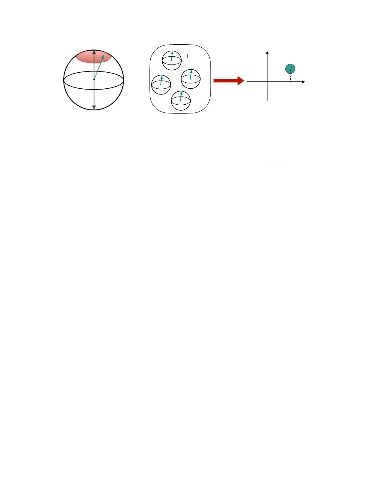
Submitted to the Annals of Statistics ASYMPTO TIC ST A TISTICAL THEOR Y OF IRREDUCIBLE QU ANTUM MARK O V CHAINS B Y F E D E R I C O G I RO T T I 1 , 2 , a , J U K K A K I U K A S 3 A N D M ˘ A D ˘ A L I N G U ¸ T ˘ A 1 , 4 1 School of Mathematical Sciences, University of Nottingham, Nottingham, NG7 2RD, United Kingdom 2 Department of Mathematics, P olytechnic University of Milan, Milan, Piazza L. da V inci 32, 20133, Italy, a federico.gir otti@polimi.it 3 Department of Mathematics, Aberystwyth University , Aberystwyth, SY23 3BZ, United Kingdom 4 Centr e for the Mathematics and Theor etical Physics of Quantum Non-equilibrium Systems, University of Nottingham, Nottingham, NG7 2RD, United Kingdom In this paper we in vestigate the asymptotic statistical theory of irre- ducible quantum Markov chains, focusing on identiﬁability properties and asymptotic con ver gence of associated quantum statistical models. W e sho w that the space of identiﬁable parameters for the stationary output is a stratiﬁed space called an orbifold, which is obtained as the quotient of the manifold of irreducible dynamics by a compact group of state preserving symmetries. W e analyse the orbifold’ s geometric properties, the connection between period- icity and strata, and provide orbifold charts as the starting point for the local asymptotic theory . The quantum Fisher information rate of the system and output state is expressed in terms of a canonical inner product on the identiﬁ- able tangent space. W e then show that the joint system–output model satisﬁes quantum local asymptotic normality while the stationary output model con- ver ges to a product between a quantum Gaussian shift model and a mixture of quantum Gaussian shift models, reﬂecting the underlying periodicity . These strong con ver gence results provide the basis for constructing asymptotically optimal estimators of dynamical parameters. W e provide an in-depth analysis of the model with smallest dimensions, consisting of two-dimensional system and en vironment units. CONTENTS 1 Introduction and summary of results . . . . . . . . . . . . . . . . . . . . . . . . . 2 1.1 Summary of results . . . . . . . . . . . . . . . . . . . . . . . . . . . . . . . 3 1.2 Structure of the paper . . . . . . . . . . . . . . . . . . . . . . . . . . . . . . 7 2 Background and preliminary results . . . . . . . . . . . . . . . . . . . . . . . . . 9 2.1 Quantum mechanics primer . . . . . . . . . . . . . . . . . . . . . . . . . . . 9 2.1.1 Postulates of quantum mechanics . . . . . . . . . . . . . . . . . . . 9 2.1.2 Quantum channels . . . . . . . . . . . . . . . . . . . . . . . . . . . 12 2.1.3 Continuous v ariables and Gaussian states . . . . . . . . . . . . . . . 13 2.2 Introduction to quantum estimation and local asymptotic normality . . . . . . 15 2.2.1 Quantum Cramér-Rao bound . . . . . . . . . . . . . . . . . . . . . . 15 2.2.2 Quantum Gaussian shift models . . . . . . . . . . . . . . . . . . . . 17 2.2.3 Quantum decision problems and comparison of quantum models . . . 20 2.2.4 Quantum local asymptotic normality . . . . . . . . . . . . . . . . . 22 2.2.5 Useful tools in proving con ver gence of statistical models . . . . . . . 25 2.3 Irreducible quantum Marko v chains . . . . . . . . . . . . . . . . . . . . . . 26 MSC2020 subject classiﬁcations : Primary 62B15, 81P50; Secondary 53B12, 57R18, 62M05, 62F12, 81S22. K e ywor ds and phrases: Quantum Statistical Inference, Irreducible Quantum Markov Chains, Identiﬁability Theory, Local Asymptotic Normality, Stratiﬁed Spaces and Orbifolds. 1 2 2.3.1 Irreducible quantum channels . . . . . . . . . . . . . . . . . . . . . 26 2.3.2 Quantum Marko v chains . . . . . . . . . . . . . . . . . . . . . . . . 29 3 Identiﬁability of stationary irreducible QMCs . . . . . . . . . . . . . . . . . . . . 30 3.1 Identiﬁability for certain classical hidden Marko v chains . . . . . . . . . . . 32 4 Global geometric structure of identiﬁable stationary irreducible QMCs . . . . . . . 33 4.1 Manifold of irreducible isometries and gauge group . . . . . . . . . . . . . . 34 4.2 Intermezzo on orbifolds . . . . . . . . . . . . . . . . . . . . . . . . . . . . . 35 4.3 Identiﬁable directions and atlas of fundamental charts . . . . . . . . . . . . . 39 4.4 Canonical stratiﬁcation . . . . . . . . . . . . . . . . . . . . . . . . . . . . . 42 5 Local approximation of stationary irreducible quantum Marko v chains . . . . . . . 44 5.1 Limit statistical models . . . . . . . . . . . . . . . . . . . . . . . . . . . . . 45 5.2 Limit results . . . . . . . . . . . . . . . . . . . . . . . . . . . . . . . . . . . 48 6 Analysis of the two-dimensional system and en vironment unit model . . . . . . . . 51 7 Conclusions and outlook . . . . . . . . . . . . . . . . . . . . . . . . . . . . . . . 60 A Proof of the results regarding the mix ed quantum Gaussian model . . . . . . . . . 61 B Proofs of lemmas on conv ergence of statistical models . . . . . . . . . . . . . . . 62 C Proof of the limit theorems for ﬂuctuation observables . . . . . . . . . . . . . . . 66 D Proof of the characterisation of the output equiv alence . . . . . . . . . . . . . . . 69 E Proofs of the results in Section 4 . . . . . . . . . . . . . . . . . . . . . . . . . . . 72 F Proofs of local approximations . . . . . . . . . . . . . . . . . . . . . . . . . . . . 74 G Proofs of Lemma 7 . . . . . . . . . . . . . . . . . . . . . . . . . . . . . . . . . . 85 References . . . . . . . . . . . . . . . . . . . . . . . . . . . . . . . . . . . . . . . . . 86 1. Introduction and summary of results. In recent decades quantum statistics has e volv ed from a theoretical challenge into a foundational principle of quantum technology that underpins adv ances in div erse areas such as state tomography [ 126 , 90 , 114 , 10 , 99 ], quantum enhanced sensing and metrology [ 58 , 51 , 47 , 46 , 158 , 133 , 119 ], quantum imaging [ 145 , 45 ], gravitational w av es detection [ 44 , 1 ] and more. In general terms, the estimation problem is to learn an unknown parameter encoded in the state of a quantum system, by performing a measurement on the system and using the outcome to compute an estimator [ 106 , 92 ]. As quantum measurements hav e probabilistic outcomes and typically disturb the system’ s state, one usually requires multiple measurements on independent ly prepared systems, a setup sim- ilar to estimation with i.i.d. models in statistics. A ke y early result in quantum estimation is the quantum Cramér -Rao bound (QCRB) for parametric models [ 96 , 15 , 92 , 106 , 25 ]. Gi ven a system prepared in a state ρ θ , the cov ariance of any unbiased estimator obtained by mea- suring the system is lower bounded by the in verse of the quantum Fisher information F θ . The latter is an intrinsic property of the quantum statistical model, which suggests that concepts and tools from “classical statistics” can be extended to the domain of quantum statistical inference. Since these early results, notable de velopments include among others the theory of quan- tum suf ﬁciency [ 130 , 103 ], the full classiﬁcation of quantum Fisher information metrics [ 132 ], the asymptotic hypothesis testing theory including quantum Stein Lemma [ 93 , 125 , 124 ] and its generalisations [ 24 , 112 , 91 ], quantum Sanov theorem [ 22 , 121 ] and quantum Chernof f bound [ 12 , 13 ], quantum decision theory [ 37 , 27 , 102 ], quantum compressed sens- ing [ 75 , 57 , 43 , 110 ], lo w rank tomography [ 108 , 151 , 31 , 9 , 29 , 85 , 139 , 4 ], quantum local asymptotic normality [ 84 , 83 , 82 , 104 , 66 , 152 , 30 , 59 , 60 , 111 ], optimal state estimation [ 84 , 66 , 122 , 123 , 88 , 155 , 60 , 156 ] and quantum semiparametrics [ 144 ]. Outside the i.i.d. setting, an important practical problem is the estimation of dynamical pa- rameters of open quantum systems undergoing Markovian e volution. An experimental setup 3 that is particularly pre valent in quantum optics is that of open systems subject to continu- ous monitoring through indirect probing of their en vironment [ 64 , 149 ]. In the continuous time setting we deal with the mathematical framew ork of quantum input-output dynamics dri ven by quantum W iener processes, which has strong connections with classical ﬁltering and control theory [ 16 , 64 , 148 , 74 , 42 ]. In this paper we in vestigate the discrete time v ersion [ 11 , 146 , 73 ], which is connected to sev eral areas such as collision models theory [ 41 ], matrix product states [ 128 , 137 ], ﬁnitely correlated states [ 54 , 56 ], and Haroche’ s one-atom maser photon-box [ 89 ]. Throughout this w ork we use the terminology of quantum Markov c hains (QMCs) which is closer to the statistical spirit of this work. The question of how to estimate dynamical parameters of quantum Marko v processes goes back to [ 115 , 61 , 19 , 134 ] with other approaches including Bayesian estimation [ 62 , 120 , 107 , 136 , 157 ], ﬁltering methods [ 135 , 36 , 138 ], quantum smoothing [ 140 , 141 , 142 , 80 ]; more recently the focus has been in ﬁnding the ultimate precision limits in terms of the quantum Fisher information [ 76 , 63 , 33 , 78 , 79 , 65 ], designing realistic optimal measurement strategies [ 71 , 70 , 153 ], and exploring the connection to enhanced metrology and dynamical phase transitions [ 116 , 6 , 7 , 100 ]. On a more fundamental statistical le vel, the identiﬁability theory , information geometry and quantum local asymptotic normality hav e been studied in [ 87 ] for irr educible continuous-time dynamics and in [ 86 ] for primitive discrete time QMCs. A ﬁrst result of these studies is that the space of identiﬁable parameters of the stationary output process is a manifold obtained by quotienting the space of dynamics by a group of system transformations which do not change the output. This is reminiscent of Petrie’ s result [ 129 ] on identiﬁability of certain classes of (classical) hidden Markov chains. The second result is that the output state model can be approximated in the sense of quantum Le Cam distance by a quantum Gaussian shift model, locally on the tangent space to the manifold of identiﬁable parameters. This is a quantum version of local asymptotic normality results for irreducible Marko v chains ([ 97 , 98 ] and references therein) and hidden Mark ov chains [ 20 , 21 ] (with the stronger requirement of primiti vity). In this work we extend the existing theory from primitiv e QMCs to irreducible ones, thus allo wing for dynamics that exhibit periodic behaviour [ 150 ]. W e ﬁnd that this seemingly minor change leads to signiﬁcantly different identiﬁcation and asymptotic statistical theory: the space of identiﬁable parameters is not a smooth manifold anymore but rather an orbifold [ 5 ] and QLAN is replaced by con ver gence to a mixtur e of quantum Gaussian shift models. While orbifolds (or stratiﬁed spaces) do appear in classical statistics, in particular in the context of mixture models [ 94 ], we are not aware of a similar analysis in the hidden Markov chains setting. W ith this in mind, for reader’ s con venience we have included a background section on quantum mechanics, estimation and QMCs and a short introduction to orbifold theory . Belo w we pro vide a high le vel summary of the concepts and results followed by an outline of the paper structure. 1.1. Summary of results. W e no w re vie w the results contained in this paper , and start by brieﬂy depicting the physical setup in vestigated here. W e consider a QMC consisting of a system with Hilbert space H = C d and initial state | φ ⟩ ∈ H , interacting successi vely with independent and identically prepared ‘environment units’ with Hilbert space K = C k , each of them being prepared in a known pure state | χ ⟩ ∈ K . The interaction is described by a unitary operator U on H ⊗ K which is applied sequentially to the system and each of the en vironment units. Since the state of the latter is ﬁxed, the dynamics is completely determined by the isometry V : H → H ⊗ K | φ ⟩ 7→ U ( | φ ⟩ ⊗ | χ ⟩ ) 4 and we will refer to this as the “dynamics”. Physically , this type of discrete-time process underlies landmark experimental setups such as Haroche’ s photon-box [ 89 ] but also mod- els general continuous-time quantum open system dynamics in the Marko v approximation, including gravitational wa ve detectors [ 14 ] and atomic clouds magnetometers [ 26 ]. From a classical perspectiv e, the dynamics bears similarities to that of a Markov chain driv en by a Bernoulli sequence [ 49 ], where the incoming en vironmental units play the role of “quan- tum coins”, while the unitary corresponds to the deterministic dynamical law governing the system’ s ev olution. An important dif ference to the classical case is that the state of the “quan- tum coin” changes due to the interaction with the system, and the system cannot be observed directly without perturbing its dynamics. After n time steps, joint system and output state is giv en by | Ψ s+o ( n ) ⟩ = V ( n ) | φ ⟩ = V ( n ) · · · V (1) | φ ⟩ where V ( j ) is the isometric embedding of the system state into that of system and the j -th en vironment unit, arising from their interaction. The right side expression implies that the system-output state is a form of matrix pr oduct state [ 128 ] where the system plays the role of memory b uilding up correlations between the output units, which is broadly similar to properties of probability distributions of classical (hidden) Markov processes. By tracing out the environment, one ﬁnds that the reduced system state (represented as a density matrix) after n steps is giv en by ρ sys ( n ) = T r out  | Ψ s+o ( n ) ⟩⟨ Ψ s+o ( n ) |  = T n ∗ ( ρ in ) , ρ in := | φ ⟩⟨ φ | where T ∗ is the system’ s one-step quantum transition operator (channel) deﬁned as T ∗ ( ρ ) = T r out ( V ρV ∗ ) . On the other hand, by tracing out the system we obtain the output state ρ out ( n, ρ in ) = T r sys  | Ψ s+o ( n ) ⟩⟨ Ψ s+o ( n ) |  . An important feature of the input-output setup of open quantum dynamics is that, instead of directly measuring the system, one learns about the dynamics by measuring the output units after the interaction with the system. In this sense quantum Marko v chains bear simi- larities to classical hidden Marko v chains, but in order to av oid confusion we will stick with the standard terminology and not use the term “hidden” in the quantum setup. The ke y assumption made throughout the paper is that the QMC is irr educible , which is equi valent to the existence of a unique strictly positiv e state ρ ss such that T ∗ ( ρ ss ) = ρ ss , called the stationary state . This has a two-fold motiv ation: on the one hand, irreducible QMCs can be considered as building blocks of more general dynamics and cov er a large number of practical e xamples; on the other hand, QMCs with multiple stationary states e xhibit radically dif ferent statistical properties such as quadratic (Heisenberg) scaling of the quantum Fisher information [ 116 ], and therefore need to be treated separately . W e stress that irreducibility is a strictly weaker assumption than primitivity as it allo ws the transition operator T ∗ to have a non-tri vial period . As we will show , this gi ves rise to signiﬁcantly different identiﬁability and asymptotic estimation theory compared to that of primitiv e QMCs [ 86 ]. A second assumption is that the output is observ ed in the stationary re gime, for which we provide three theoretical moti vations in section 3 . The quantum statistical problem under in vestigation is the following: gi ven a QMC with unkno wn unitary dynamics, we would lik e to estimate the dynamics (or a parameter thereof) by performing measurements on the (stationary) output units and using the outcomes to com- pute an estimator . More speciﬁcally , we would like to kno w which dynamical parameters are identiﬁable, and ho w well they can be estimated in the lar ge time limit regime. 5 T o answer the ﬁrst question we deﬁne an equiv alence relation between irreducible dy- namics with identical stationary output states and characterise the corresponding equiv alence classes. Let V irr denote the set of isometries of irreducible QMCs. T wo isometries V 1 , V 2 are called output equivalent if they have the same stationary output states, i.e. ρ out V 1 ( n ) = ρ out V 2 ( n ) for all n ≥ 1 . The equiv alence relation is completely characterised in Theorem 6 , which we reproduce here informally for con venience. Result 1. (output equivalence) T wo isometries V 1 , V 2 ar e output equivalent if and only if ther e exists a unitary W on H and a phase e iϕ ∈ C such that V 2 = e iϕ ( W ⊗ 1 K ) V 1 W ∗ . The space of identiﬁable parameters P irr is therefore the set of equiv alence classes of isometries [ V ] gi ven by the orbit of V under the action of the group G = U (1) × P U ( d ) acting on V irr , cf. equation ( 37 ). Passing from V irr to P irr comes at the price of gi ving up the manifold structure of V irr and ha ving to deal with a quotient space, which, a priori is deﬁned in a rather implicit way . This issue is resolved in Theorem 10 which sho ws that P irr has the structure of an orbifold, which loosely speaking means a topological space that can be locally identiﬁed with the quotient of a subset of the Euclidean space under the action of a ﬁnite group of smooth transformations. The key ingredient is Theorem 8 which identiﬁes the the stabiliser group of G V of a dynamics V with the set of pairs { ( γ k V , Z k v ) : k = 0 , . . . , p V − 1 } of peripheral eigen values and unitary eigen vectors of the transition operator T V . Result 2. (orbifold structure) The space of identiﬁable parameters P irr has a natural orbifold structur e inherited fr om the action of the compact Lie gr oup G over the manifold of dynamical parameter s V irr . The theory of orbifolds [ 32 ] allows us to deriv e sev eral geometric properties of P irr : com- pute its dimension, e xpress it as a disjoint union of manifolds (called singular manifolds ), de- scribe the connected components of such submanifolds and analyse ho w such submanifolds sit together inside the orbifold. Using these tools we construct an atlas of orbifold charts that turns out to be a valuable tool in the study of the asymptotic statistical theory of QMCs. In brief, the tangent space T V ( V irr ) to V irr at a point V decomposes as the direct sum T V ( V irr ) = T nonid V ⊕ T id V , where T nonid V is the space of non-identiﬁable directions consisting of tangent v ectors to the orbits of G , and T id V is the space of identiﬁable directions consisting of bounded linear op- erators A : H → H ⊗ K satisfying V V ∗ A = 0 , cf Proposition 4 . The space T id V is naturally endo wed with a complex structure and carries the inner product ( A, B ) V = T r( ρ ss V A ∗ B ) , which plays an important role in deﬁning the dif ferent limit statistical models. The space T id V also carries a unitary representation π V of the discrete stabiliser group G V which is intimately related to the unitary eigen vectors of the transition operator T V corresponding to peripheral eigen values. The quotient of T id V by this action is the tangent cone to the orbifold P irr and describes an inﬁnitesimal neighbourhood of [ V ] . Let us now consider the problem of estimating the dynamics V from (system and) output measurements. According to the quantum Cramér-Rao bound, the covariance of any (locally) unbiased estimator is larger than the in verse of the quantum Fisher information (QFI) of the model. For the system and output state | Ψ s+o V ( n ) ⟩ we show that the QFI F s+o V ( n ) scales linearly with respect to time for directions in the identiﬁable space T id V and is bounded for the non-identiﬁable directions in T nonid V . Proposition 6 shows that the scaling f actor is given by the real part of the inner product on T id V deﬁned earlier . 6 Result 3. (QFI rate for identiﬁable parameters) Let A = A id + A nonid , B = B id + B nonid be the decompositions into identiﬁable and non-identiﬁable components of A, B ∈ T V . Then the QFI rate at V is giv en by lim n →∞ 1 n F s+o V ,n ( A, B ) = 4Re ( A id , B id ) V . Going beyond QFI, we show that the sequence of stationary system and output quantum models | Ψ s+o V ( n ) ⟩ con ver ges in the Le Cam sense (see Deﬁnition 2 ) to a quantum Gaussian shift model, i.e. it satisﬁes quantum local asymptotic normality (QLAN). T o formulate this, let us consider a ﬁxed parameter V 0 ∈ V irr and the system and output state | Ψ s+o V ( n ) ⟩ corre- sponding to a parameter V = V 0 + n − 1 / 2 A where A ∈ T id V 0 is a “local parameter” whose magnitude is allowed to grow slowly as n δ for 0 < δ < 1 / 2 . Let us use the above geo- metric data to deﬁne the limit quantum model which consists of Gaussian (coherent) states | Coh( A ) ⟩ := W ( A ) | Ω ⟩ of a continuous v ariables system, where W ( A ) are W eyl operators of the canonical commutations relations algebra C C R ( T id V 0 , ( · , · ) V 0 ) deﬁned by W ( A ) W ( B ) = e − i Im( A,B ) V 0 W ( A + B ) , A, B ∈ T id V 0 and | Ω ⟩ is the “vacuum” state with characteristic function ⟨ Ω | W ( A ) | Ω ⟩ = e − ( A,A ) V 0 2 . The following result shows the Le Cam conv ergence of the system and output models to the Gaussian shift model ov er gro wing local neighbourhoods (cf. Theorem 11 ). Result 4. (QLAN for system and output state) For any giv en V 0 ∈ V irr , the system and output state satisﬁes QLAN. Concretely , for δ small enough, there exist quantum channels F s+o n , B s+o n such that sup ∥ A ∥≤ n δ ∥F s+o n ( ρ s+o A,n ) − G ( A ) ∥ 1 = o ( n − 2 δ ) , sup ∥ A ∥≤ n δ ∥ ρ s+o A,n − B s+o n ( G ( A )) ∥ 1 = o ( n − 2 δ ) , where ρ s+o A,n = | Ψ s+o V 0 + n − 1 / 2 A ( n ) ⟩⟨ Ψ s+o V 0 + n − 1 / 2 A ( n ) | and G ( A ) = | Coh( A ) ⟩⟨ Coh( A ) | . Note that the QLAN result is operational in the sense that it prescribes physical transfor- mations connecting the models, and strong in the sense that it pro vides con ver gence rates for the deﬁciency between the models, while the latter are allowed to grow locally . Note also that the same result holds for “full” neighbourgoods of V 0 including non-indentiﬁable directions, but the limit remains dependent only on the identiﬁable component. Let us consider no w the stationary output state ρ out V ( n ) . Result 2. showed that the state depends only on the equi valence class [ V ] so the model should be seen as being parametrised by points in the space P irr . In Theorem 12 we sho w that the sequence of stationary output quantum models ρ out V ( n ) con ver ges in the Le Cam sense to a limit quantum model, locally in the space of identiﬁable parameters. Remarkably , unlike the case of primitiv e (aperiodic) dynamics, the limit model is not a quantum Gaussian shift model but rather a mixture of Gaussian models which are related to each other by the unitary action of a discrete group. In particular , quantum local asymptotic normality does not hold in the vecinity of periodic QMCs. T o deﬁne the limit model consider the algebra C C R ( T id V 0 , ( · , · ) V 0 ) introduced earlier and deﬁne the mixture of coherent states ρ ( A ) := 1 p [ V 0 ] X g ∈ G V 0 | Coh( U V 0 ( g ) A ) ⟩⟨ Coh( U V 0 ( g ) A ) | , 7 where U V 0 ( g ) is the unitary representation of G V 0 on T id V 0 . Physically , this amounts to aver - aging the coherent state | Coh( A ) ⟩⟨ Coh( A ) | by the action of the second quantisation of the unitary group { U V 0 ( g ) k } p [ V 0 ] k =0 on T id V 0 . Note that this model is different from those obtained in quantum versions of local asymptotic mixed normality [ 18 ] where one has access to the label of the indi vidual components of the mixture. Theorem 12 is informally stated as follows. Result 5. (Limit mixtur e of quantum Gaussian shift models) Let V 0 ∈ V irr be ﬁxed and consider the sequence of local output models ρ out A,n := ρ out [ V 0 + n − 1 / 2 A ] ( n ) with local parameter A ∈ T id V 0 . Then, for δ small enough, there exist quantum channels F out n , B out n such that sup ∥ A ∥≤ n δ ∥F out n ( ρ out A,n ) − ρ ( A ) ∥ 1 = o ( n − 2 δ ) , sup ∥ A ∥≤ n δ ∥ ρ out A,n − B out n ( ρ ( A )) ∥ 1 = o ( n − 2 δ ) . Results 4 and 5 put the basis of an asymptotic estimation theory for QMCs. In classi- cal asymptotics, it is well known that such strong conv ergence results can be used to deriv e asymptotic minimax rates of con ver gence [ 113 ], and similar techniques have been demon- strated in the quantum setup in [ 84 , 30 , 155 ] for i.i.d. models. A detailed analysis of the estimation theory is left for a future work. Result 6. (W orked out example) In the ﬁnal part of the paper we apply the general theory de veloped here to the class of QMCs with two dimensional system and en vironmental units, i.e. H = K = C 2 . The space of isometries V irr has dimension 12 and its quotient by the group G is an orbifold P irr made up of an 8 dimensional manifold P prim and a 4 dimensional sub- manifold P 2 , 4 of dynamics with period 2 . For the purpose of illustration, a cartoon version of this geometry is represented in panels a) and b) of Figure 1 . In the neighbourhood of primi- ti ve dynamics the output model satisﬁes QLAN with a 4-modes limit quantum Gaussian shift model. In contrast, the asymptotic behaviour near periodic points has a richer , more inter- esting structure. The identiﬁable tangent space T id V at a periodic point V decomposes into 2 subspaces V 0 , V 1 of (complex) dimension 2 which are eigenspaces of the stabiliser with eigen values 1 and respecti vely − 1 . This means that the limit model is a product between a 2-mode Gaussian shift model corresponding to mov ement within the periodic submanifold P 2 , 4 , and a 2-mode Gaussian mixture model for direction away from the singular manifold. W e analyse 3 one-dimensional models passing through a periodic point, whose (identiﬁable) tangent vectors lie in V 1 , V 0 or neither (labelled as (I), (II), (III) in Figure 1 b)). In the latter two cases we pro vide output measurement and estimation procedures which “localise” the parameter at standard rate; in the third case we show that the signal to noise ratio (SNR) of av erage statistics for simple repeated measurements v anishes near the periodic point, while the SNR for certain joint measurements on pairs of en vironmental units remains non-zero in this limit. This analysis suggest that parameters can be estimated at standard rate in a preliminary localisation stage, and thus provides the basis for a future in vestigation into the asymptotic minimax theory of QMCs, combining preliminary estimation with the asymptotic approximation results derived here, in the spirit of the works [ 155 , 28 ] in the i.i.d. setting. Figure 1 c) illustrates the three corresponding limit Gaussian and mixed Gaussian statistical experiments. 1.2. Structur e of the paper . In section 2 we pro vide a brief introduction to concepts and results used in this work, such as fundamental notions of quantum mechanics, quantum esti- mation theory and quantum Marko v chains. Section 3 deals with the identiﬁability problem for irreducible QMCs. Three statistical tasks are presented and the corresponding notions of 8 F I G 1 . Conceptual r epr esentation of the local geometry of stationary QMCs with two dimensional system and ancillas, and limit quantum statistical models for 3 one-parameter models. P anel a) depicts the (12 dimensional) manifold of isometries V irr and the action of the symmetry group G . Locally , the action consists of translations along the Z axis together with the Z 2 action of r eﬂections ar ound the X Z plane that r epresents periodic QMCs. The blue arr ows correspond to the transformations generating the gr oup, while the two vertical red lines constitute a single arbitrarily chosen orbit. At every point, the non-identiﬁable tangent space T nonid consists of vectors in the Z direction while T id is parallel to the X Y plane. The latter carries the action of the stabiliser group Z 2 and decomposes into the dir ect sum of eigenspaces V 0 and V 1 consisting of vectors along the X and r espectively the Y axis. P anel b) r epr esents the orbifold obtained as the quotient of V irr under the action of G , which can be identiﬁed with the X Y plane folded along the X axis, repr esented as a half plane including the ‘edge’ axis X ; the axis corresponds to the (4 dimensional) manifold P 2 , 4 of equivalence classes of periodic isometries, while the plane repr esents the (8 dimensional) manifold P prim of equivalence classes of primitive QMCs. The red dot corresponds to the orbit repr esented by red lines in a ) . W e analyse the asymptotics of three one-dimensional models with distinct geometries and limit models. In the parameter space these ar e the following lines in the X Y plane: a line (I) along the X axis, a line (II) which is non-orthogonal to either X or Y axis, and a line (III) parallel to the Y axis. F or clarity , the lines ar e not repr esented in panel a) b ut their orbifold pr ojections ar e repr esented in panel b) by purple arrows: (I) lies inside the singular manifold, (II) is the ‘br oken’ line that cr osses the singular manifold in one point, and (III) is a half line in the Y dir ection, e xhibiting non-identiﬁability . P anel c ) r eports a repr esentation in the phase space of the limit quantum statistical models corresponding to the thr ee one-parameter models, locally ar ound a point at the intersection with the X axis (periodic QMC). Orange cir cles r epresent quantum coher ent states with standar d vacuum co variance. (I) is a pur e quantum Gaussian shift model where the mean moves along the Q axis. (II) is the tensor product of a pure Gaussian shift model as the one consider ed in (I) and a mixture of two coher ent states with opposite means: the means move together when the local parameter chang es. Finally , the third model is described by a mixture of coher ent states lying on the Q axis with opposite means. W e remark that the local par ameter is identiﬁable in (I) and (II), but not in (III). identiﬁability are deﬁned in Deﬁnitions 4 , 6 and 5 ; these are showed to be equiv alent using Lemma 4 , which is of independent interest. The equiv alence class of QMCs with identical 9 stationary outputs is completely characterized in Theorem 6 . In Section 4 we further elabo- rate on the identiﬁability theory and sho w that the equiv alence classes are orbits of a group acting smoothly on the manifold of irreducible QMCs (Theorem 8 ); moreov er , in the same Theorem we sho w that the action satisﬁes the requirements for the quotient space to be en- do wed with the structure of an orbifold. Section 4.2 contains a reminder of all the notions and results about orbifolds used in the paper . In Section 4.3 we construct an orbifold atlas for the parameter space which turns out to be a con venient parametrization for the results in Section 5 . Section 4.2 treats the decomposition of P irr into submanifolds and discusses some of their properties (Proposition 5 ). Theorems 11 and 12 in Section 5.2 provide local approximations of the statistical models corresponding to the system and output state and the stationary output state, respectively . Corollary 2 determines exactly those cases in which LAN holds. Section 6 applies the general theory to the class of QMCs with two-dimensional system and en vironment unit. 2. Background and pr eliminary results. Quantum theory employs the mathematical frame work of linear operators on complex Hilbert spaces to describe physical phenomena at the microscopic scale of atoms and photons. One of the key features of the theory is that quan- tum measurements are intrinsically pr obabilistic , so that the problem of learning the state of a system is fundamentally of a statistical nature. Such problems have become ubiquitous in Quantum T echnology where experimenters use statistical inference to reconstruct parameters of quantum states and devices for validation purposes, but also to estimate unknown phys- ical quantities with high precision. In this section we give a brief introduction to the basic concepts and techniques of the ﬁeld, and highlight a new technical tool on con ver gence of quantum models which has a wider applicability . 2.1. Quantum mec hanics primer . In this section we giv e a condensed introduction to the basic notions of quantum mechanics leading to the theory of quantum channels and Gaussian states which play a ke y role later on. 2.1.1. P ostulates of quantum mechanics. In quantum mechanics, each system (e.g. par - ticle, electromagnetic ﬁeld) is described mathematically in terms of a separable, complex Hilbert space H , and certain linear operators acting on it. In this paper we adopt the physi- cists (Dirac) notation, whereby a v ector ψ in a Hilbert space H is denoted by using the “k et” symbol | ψ ⟩ , while the “bra” vector ⟨ ϕ | denotes the adjoint ϕ ∗ , such that the inner product between | ϕ ⟩ and | ψ ⟩ is denoted ⟨ ϕ | ψ ⟩ . W e denote by L ∞ ( H , K ) the space of bounded operators deﬁned on H and taking v alues in K ; if H = K , we will use the simpler notation L ∞ ( H ) . W e consider L ∞ ( H ) equipped with the operator norm ∥ X ∥ ∞ = sup ∥ ψ ∥ H =1 ∥ X ψ ∥ K and we let L 1 ( H ) be the space of trace-class operators, i.e. bounded operators τ satisfying ∥ τ ∥ 1 := T r( | τ | ) < ∞ where | τ | = √ τ ∗ τ is the absolute v alue (operator) and τ ∗ is the adjoint of τ . Any bounded linear functional on L 1 ( H ) takes the form τ ∈ L 1 ( H ) 7→ T r( ρX ) ∈ C for some bounded operator X , so that L ∞ ( H ) is the dual of L 1 ( H ) . This fundamental duality is the quantum analogue of the duality encountered in probability theory between the space of absolutely integrable functions L 1 (Ω , Σ , µ ) and that of bounded measurable functions L ∞ (Ω , Σ , µ ) , where (Ω , Σ , µ ) is a probability space. Quantum states. The state of a quantum system with Hilbert space H incorporates infor - mation about its preparation and is represented mathematically by a density matrix , i.e. an 10 operator in L 1 ( H ) which is positiv e and has trace one. The space of states S ( H ) ⊂ L 1 ( H ) is conv ex and its e xtremal elements are the pur e states represented by one-dimensional pro- jections P ψ = | ψ ⟩⟨ ψ | where | ψ ⟩ is a unit v ector . When dealing with pure states we will often work with the vectors themselves rather than the projections and refer to | ψ ⟩ as being the “state”, or the “wav e function” of the system. In general, a state ρ ∈ S ( H ) which is not pure is called mixed and can be written as a con ve x combinations of pure states. One such representation is gi ven by the spectral decomposition ρ = X i λ i | e i ⟩⟨ e i | where λ i are the eigen values of ρ and | e i ⟩ are the corresponding eigen vectors. The positi vity and trace properties of ρ imply that { λ i } i is a discrete probability distribution. Observables. In quantum mechanics, the system’ s observables are represented by selfadjoint operator s acting on its Hilbert space H . According to the Spectral Theorem, any observable has a spectral decomposition of the form (1) A = Z σ ( A ) λP ( dλ ) where σ ( A ) ⊂ R is the spectrum of A and P ( dλ ) is the associated pr ojection valued measur e whose elements are orthogonal projections. More precisely , P : Σ → L ∞ ( H ) is a map from the Borel σ -algebra of σ ( A ) to bounded operators such that 1. P ( E ) = R E P ( dλ ) is an orthogonal projection for each E ∈ Σ ; 2. P is σ -additiv e, i.e. P ( S i E i ) = P i P ( E i ) for disjoint sets { E i } i in Σ ; 3. P ( ∅ ) = 0 and P ( σ ( A )) = 1 . For ﬁnite dimensional spaces, observables have discrete spectrum gi ven by the set of eigen- v alues, and the spectral projections are the corresponding eigenprojectors. The duality between L 1 ( H ) and L ∞ ( H ) provides us with a quantum notion of e xpectation. For any state ρ and any bounded observ able A , we deﬁne the expected value of the latter with respect to the former by T r( ρA ) . Its full probabilistic interpretation is described below in the context of measurements. Measur ements. Measurements provide the link between the quantum world of “wa ve func- tions” and the classical one of stochastic measurement outcomes. In its most general form, a measurement with outcomes in a measure space (Ω , Σ , µ ) is described by a bounded linear transformation M ∗ : L 1 ( H ) → L 1 (Ω , Σ , µ ) which maps a state ρ into the probability density p M ρ := M ∗ ( ρ ) with respect to the gi ven reference measure µ . When the measurement is performed on a system in state ρ , one obtains a sample X from the distribution P M ρ with density p M ρ . For each E ∈ Σ , the dual map M : L ∞ (Ω , Σ , µ ) → L ∞ ( H ) deﬁnes the positive operator M ( E ) := M ( χ E ) where χ E is the characteristic function of E . The collection { M ( E ) : E ∈ Σ } is called a positive oper ator valued measur e (PO VM) and determines the probability distribution of the measurement outcomes P M ρ ( E ) = T r( ρM ( E )) . Note that, as a map from states to probability densities, the measurement can be regarded as a quantum-to-classical randomisation, in analogy to classical-to-classical randomisations 11 R : L 1 (Ω 1 , Σ 1 , µ 1 ) → L 1 (Ω 2 , Σ 2 , µ 2 ) which map probability densities to probability densi- ties. The most common type of measurement is that associated to an observable. When mea- suring the observ able A with spectral decomposition ( 1 ) on a system in state ρ , we obtain a random outcome a ∈ σ ( A ) with probability distrib ution P ρ ( a ∈ E ) = T r( ρP ( E )) , E ∈ Σ . In this case the PO VM is gi ven by the projection v alued measure associated to the spectral decomposition of A . In particular, the e xpected value of the outcome X is E ρ ( X ) = Z σ ( A ) a T r( ρP ( da )) = T r( ρA ) . Unitary tr ansformations. The time e volution of a closed quantum system H is determined by a unitary operator U ∈ L ∞ ( H ) , so that an initial v ector state | ψ ⟩ is transformed into the ﬁnal state U | ψ ⟩ . On the level of density matrices, this action becomes that of unitary conjug ation U ∗ : L 1 ( H ) → L 1 ( H ) ρ 7→ U ρU ∗ . This description of the e volution is often called the Schrödinger pictur e , where states change and observ ables are ﬁxed in time. An alternative view is the Heisenberg pictur e where the system’ s state is always ﬁx ed but observ ables ev olve according to the dual map U : L ∞ ( H ) → L ∞ ( H ) X 7→ U ∗ X U The two pictures are equiv alent in the sense that they both described the same expected values of observ ables and measurement probabilities T r [ U ∗ ( ρ ) A ] = T r [ ρ U ( A )] , A ∈ L ∞ ( H ) , ρ ∈ L 1 ( H ) . This is similar to the treatment of dynamics in stochastic processes where the ev olution can be described in terms of time changing random v ariables or probability distributions. Composite systems. The Hilbert space of a composite system consisting of a ﬁnite number of sub-systems with Hilbert spaces H 1 , . . . , H k , is given by the tensor pr oduct H = N k i =1 H i . States of the form ρ = N k i =1 ρ i are called pr oduct states and correspond to individual systems being prepared independently in states ρ 1 , . . . , ρ k . Con ve x combinations of such states are called separable while all other states are called entangled . In particular , pure (vector) states are either of the product form N k i =1 | ψ i ⟩ or they are entangled. States over multipartite systems are quantum analogues of joint distributions of sev- eral random variables. If ρ 12 is a density matrix on the bipartite space H 1 ⊗ H 2 then its mar ginals represent the states of the subsystems H 1 and H 2 and are giv en by the partial traces ρ 1 := T r 2 ( ρ 12 ) and ρ 2 := T r 1 ( ρ 21 ) . As in the classical case, the marginals deter- mine the expectations of observ ables corresponding to individual sub-subsystems: indeed if A ∈ L ∞ ( H 1 ) and B ∈ L ∞ ( H 2 ) then their e xpectations can be computed as T r 1 ( ρ 1 A ) = T r 12 ( ρ 12 ( A ⊗ 1 2 )) , T r 2 ( ρ 2 B ) = T r 12 ( ρ 12 ( 1 1 ⊗ B )) . where A ⊗ 1 2 denotes the ampliation of A by the identity operator 1 2 on H 2 . 12 System Environment U ⇤ AAAB+nicbVDLSsNAFL3xWesr1aWbwVYQFyUpii6LblxWMG2hDWEynbZDJw9mJkqJ+RQ3LhRx65e482+ctFlo64GBwzn3cs8cP+ZMKsv6NlZW19Y3Nktb5e2d3b19s3LQllEiCHVIxCPR9bGknIXUUUxx2o0FxYHPacef3OR+54EKyaLwXk1j6gZ4FLIhI1hpyTMrtX6A1ZhgnjqZl55lNc+sWnVrBrRM7IJUoUDLM7/6g4gkAQ0V4VjKnm3Fyk2xUIxwmpX7iaQxJhM8oj1NQxxQ6aaz6Bk60coADSOhX6jQTP29keJAymng68k8p1z0cvE/r5eo4ZWbsjBOFA3J/NAw4UhFKO8BDZigRPGpJpgIprMiMsYCE6XbKusS7MUvL5N2o26f1y/uGtXmdVFHCY7gGE7Bhktowi20wAECj/AMr/BmPBkvxrvxMR9dMYqdQ/gD4/MHt/iTpw== ⌧ AAAB7XicbVDLTgJBEOzFF+IL9ehlIph4IrtEo0eiF4+YyCOBDZkdZmFkdmcz02tCCP/gxYPGePV/vPk3DrAHBSvppFLVne6uIJHCoOt+O7m19Y3Nrfx2YWd3b/+geHjUNCrVjDeYkkq3A2q4FDFvoEDJ24nmNAokbwWj25nfeuLaCBU/4DjhfkQHsQgFo2ilZrmLNC33iiW34s5BVomXkRJkqPeKX92+YmnEY2SSGtPx3AT9CdUomOTTQjc1PKFsRAe8Y2lMI278yfzaKTmzSp+EStuKkczV3xMTGhkzjgLbGVEcmmVvJv7ndVIMr/2JiJMUecwWi8JUElRk9jrpC80ZyrEllGlhbyVsSDVlaAMq2BC85ZdXSbNa8S4ql/fVUu0miyMPJ3AK5+DBFdTgDurQAAaP8Ayv8OYo58V5dz4WrTknmzmGP3A+fwDcdY6q T ⇤ ( ⇢ ) AAAB/nicbVDLSgMxFM3UV62vUXHlJtgK1UWZKYoui25cVugLOsOQSdM2NJMMSUYoQ8FfceNCEbd+hzv/xkw7C60eCBzOuZd7csKYUaUd58sqrKyurW8UN0tb2zu7e/b+QUeJRGLSxoIJ2QuRIoxy0tZUM9KLJUFRyEg3nNxmfveBSEUFb+lpTPwIjTgdUoy0kQL7qOJFSI8xYmlrFpxXPTkWZ5XALjs1Zw74l7g5KYMczcD+9AYCJxHhGjOkVN91Yu2nSGqKGZmVvESRGOEJGpG+oRxFRPnpPP4MnhplAIdCmsc1nKs/N1IUKTWNQjOZZVXLXib+5/UTPbz2U8rjRBOOF4eGCYNawKwLOKCSYM2mhiAsqckK8RhJhLVprGRKcJe//Jd06jX3onZ5Xy83bvI6iuAYnIAqcMEVaIA70ARtgEEKnsALeLUerWfrzXpfjBasfOcQ/IL18Q3l15TM ⇢ AAAB7XicbVBNSwMxEJ2tX7V+VT16CbaCp7JbFD0WvXisYD+gXUo2zbax2WRJskJZ+h+8eFDEq//Hm//GbLsHbX0w8Hhvhpl5QcyZNq777RTW1jc2t4rbpZ3dvf2D8uFRW8tEEdoikkvVDbCmnAnaMsxw2o0VxVHAaSeY3GZ+54kqzaR4MNOY+hEeCRYygo2V2tW+GsvqoFxxa+4caJV4OalAjuag/NUfSpJEVBjCsdY9z42Nn2JlGOF0VuonmsaYTPCI9iwVOKLaT+fXztCZVYYolMqWMGiu/p5IcaT1NApsZ4TNWC97mfif10tMeO2nTMSJoYIsFoUJR0ai7HU0ZIoSw6eWYKKYvRWRMVaYGBtQyYbgLb+8Str1mndRu7yvVxo3eRxFOIFTOAcPrqABd9CEFhB4hGd4hTdHOi/Ou/OxaC04+cwx/IHz+QPa846p F I G 2 . Quantum channel as a black box transformation mapping the initial system state ρ to ﬁnal state T ∗ ( ρ ) thr ough the unitary interaction with an en vir onment system in a ﬁxed initial state τ . 2.1.2. Quantum channels. In practice, quantum systems are nev er perfectly isolated b ut interact with their en vironment, so ev en though the full system-en vironment ev olution may be unitary , the marginal state of the system does not transform unitarily . Instead, such trans- formations are described by a class of maps called quantum c hannels on which we focus our attention at the end of this section. These can be seen as quantum-to-quantum randomisations but also as quantum analogue of transition matrices for Mark ov chains, as we will see later . W e introduce this notion through the example of a system H interacting with the en vi- ronment K via a unitary U acting on H ⊗ K , cf. Figure 2 . If the two systems are indepen- dent and hav e initial states | φ ⟩ ∈ H and respectively | χ ⟩ ∈ K then the ﬁnal joint state is | Ψ ⟩ := U | φ ⊗ χ ⟩ . By expanding with respect to an orthonormal basis {| 1 ⟩ , . . . , | k ⟩} in K we write | Ψ ⟩ = k X i =1 K i | φ ⟩ ⊗ | i ⟩ where K i = ⟨ i | U | χ ⟩ ∈ L ∞ ( H ) are operators satisfying P k i =1 K ∗ i K i = 1 H , and the inner product is with respect to K . The marginal system state (density matrix) after the e volution is ρ sys ′ = T r K ( U ( ρ sys ⊗ τ ) U ∗ ) = k X i =1 K i | φ ⟩⟨ φ | K ∗ i where ρ sys := | φ ⟩⟨ φ | and τ := | χ ⟩⟨ χ | are the initial states of system and en vironment. W e no w extend this argument to arbitrary system states and express the state transformation as the map which in the Schrödinger picture is gi ven by (cf. Figure 2 ) T ∗ : L 1 ( H ) → L 1 ( H ) T ∗ : ρ 7→ T r K ( U ( ρ ⊗ τ ) U ∗ ) = k X i =1 K i ρK ∗ i . Remarkably , it turns out that any physical transformation is of the above form. Indeed, if we consider a system under going a generic black-box transformation T ∗ : L 1 ( H ) → L 1 ( H ) , then on physical grounds it is natural to require T ∗ to map states into states and to preserve con ve x combinations; this means that T ∗ should be linear , positi ve ( T ∗ ( A ) ≥ 0 for A ≥ 0 ) and trace preserving. Moreov er , by applying a similar ar gument to the composite system C n ⊗ H where the n -dimensional auxiliary system undergoes the identity transformation I n ∗ , we conclude that I n ∗ ⊗ T ∗ must be positi ve for all n ∈ N . A map T ∗ with this property is called completely positive (CP). This requirement is a strictly stronger than positivity as it can be shown that certain maps (e.g. transposition) are positi ve b ut not completely positi ve. 13 The follo wing theorem [ 109 , 40 ] sho ws that all physical state transformations can be re- alised by coupling the system with an “en vironment” via a unitary transformation and tracing out the en vironment, as in our motiv ating example, cf. Figure 2 . T H E O R E M 1 ( Kraus Theorem) . A linear map T ∗ : L 1 ( H ) → L 1 ( H ) is completely posi- tive and trace pr eserving if and only if it is of the form T ∗ ( ρ ) = ∞ X i =1 K i ρK i for a set of operator s K i ∈ L ∞ ( H ) satifying P ∞ i =1 K ∗ i K i = 1 H (wher e the con ver gence holds in the str ong operator topology). Such a map (and its dual T : L ∞ ( H ) → L ∞ ( H ) ) is called a quantum channel. 2.1.3. Continuous variables and Gaussian states. The term continuous variables (CV) system refers to a quantum system whose fundamental observables are quantum mechani- cal v ersions of canonical coordinates and momenta associated to degrees of freedom of a classical mechanical system. In a physical context, these observables are often position and momentum operators of free particles, or electric and magnetic components of a number of monochromatic modes of the electromagnetic ﬁeld. In a quantum statistical context, such systems emerge from the asymptotic analysis of estimation problems where the limit model is described by a CV system whose state is a quantum analogue of a Gaussian distribution. W e refer to [ 106 , 127 ] for the material presented below . W e start with an arbitrary complex Hilbert space ( X , ⟨·|·⟩ ) of ﬁnite dimension k , which we refer to as the one-particle space. If we regard X as a real linear space of dimension 2 k (called the phase space ) we can deﬁne the real inner product β , and the bilinear symplectic form σ as β ( x, y ) = Re ⟨ x | y ⟩ , σ ( x, y ) = Im ⟨ x | y ⟩ . No w we deﬁne the symmetric F ock space H ( X ) = C | Ω ⟩ ⊕ ∞ M n =1 X ⊗ s n , where X ⊗ s n denotes the symmetric subspace of X ⊗ n , often called the n -particle space, and C | Ω ⟩ is a a one-dimensional space generated by the vector | Ω ⟩ called the vacuum . For each | x ⟩ ∈ X we deﬁne the exponential vectors | e x ⟩ = ∞ M n =0 1 √ n ! | x ⟩ ⊗ n ∈ H ( X ) , where we denote | x ⟩ ⊗ 0 = | Ω ⟩ (so that | e 0 ⟩ = | Ω ⟩ ). The exponential vectors span the Fock space H ( X ) , and satisfy ⟨ e x | e y ⟩ = e ⟨ x | y ⟩ for all x, y ∈ X . W e further deﬁne the unitary W eyl operator s by their action on exponential v ectors as (2) W ( x ) | e y ⟩ = e − 1 2 ∥ x ∥ 2 −⟨ x | y ⟩ | e x + y ⟩ , x, y ∈ X . From this it follo ws that (3) W ( x ) ∗ = W ( − x ) , W ( x + y ) = e iσ ( x,y ) W ( x ) W ( y ) , x, y ∈ X , which implies that x 7→ W ( x ) is a projectiv e representation of the group of phase space translations on H ( X ) . 14 While the W eyl operators implement phase space translations, we can also represent phase space rotations by means of second quantisation operators. If U is a unitary on X , its second quantisation Γ[ U ] is deﬁned as a unitary operator on H ( X ) with the follo wing action on exponential v ectors: Γ[ U ] | e x ⟩ = | e U x ⟩ . In particular , the action of Γ[ U ] restricted to the n -particle space is gi ven by U ⊗ n . This induces an automorphism α U on L ∞ ( H ( X )) deﬁned by (4) A ∈ L ∞ ( H ( X )) 7→ α U ( A ) = Γ[ U ] A Γ[ U ] ∗ In particular , α U ( W ( x )) = W ( U x ) for all x ∈ X , and since Γ[ U ] | Ω ⟩ = | Ω ⟩ , we obtain Γ[ U ] W ( x ) | Ω ⟩ = W ( U x ) | Ω ⟩ . For each x ∈ X , consider the unitary representation R ∋ t 7→ W ( tx ) of the abelian group R ; by Stone-von Neumann Theorem, the group has a selfadjoint generator Z ( x ) , so that W ( tx ) = exp( − itZ ( x )) . The operators Z ( x ) are called quadratur es , and are the quan- tum analogues of the classical phase space position and momentum v ariables. Howe ver , the quadratures do not commute in general and instead satisfy the following canonical commu- tation r elations (CCR) which can be derived from ( 3 ) (5) Z ( x ) Z ( y ) − Z ( y ) Z ( x ) = 2 iσ ( x, y ) 1 . Let X = X 1 ⊕ X 2 be a decomposition of X into two orthogonal closed subspaces and note that the map | e x 1 ⟩ ⊗ | e x 2 ⟩ 7→ | e x 1 ⊕ x 2 ⟩ can be extended linearly to a unitary V X 1 ,X 2 : H ( X 1 ) ⊗ H ( X 2 ) → H ( X 1 ⊕ X 2 ) . Bearing this in mind, it is con venient to make the identiﬁcations H ( X 1 ⊕ X 2 ) = H ( X 1 ) ⊗ H ( X 2 ) , | e x 1 ⊕ x 2 ⟩ = | e x 1 ⟩ ⊗ | e x 2 ⟩ , (6) where for simplicity we omitted the unitary V X 1 ,X 2 . From this we derive the following rela- tion for the W eyl operators W ( x 1 ⊕ x 2 ) = W ( x 1 ) ⊗ W ( x 2 ) , x 1 ∈ X 1 , x 2 ∈ X 2 . In particular , if { e j : j = 1 , . . . , k } is an orthonormal basis in X then the Fock space decom- poses into a tensor product of “one-mode" Fock spaces H ( X ) = ⊗ k j =1 H ( C e j ) and for each x = P k j =1 x k e j we hav e W ( x ) = ⊗ k j =1 W ( x j e j ) . The associated generators pairs Q j := Z ( − ie j ) , P j := Z ( e j ) act on the j th terms of the tensor product and as identity on the others, and form a basis for quadratures, playing the role of “position” and “momentum” of the k modes speciﬁed by the basis. In this representation the canonical variables satisfy the commutation relations [ Q i , P j ] = 2 iδ ij 1 , as a consequence of ( 5 ). The corresponding classical variables are then chosen to form the symplectic basis { e 1 , ie 1 , e 2 , ie 2 , . . . , e k , ie k } of the (real linear) phase space X , which is then identiﬁed with R 2 k so that the natural basis { e 1 , . . . , e 2 k } corresponds to the abo ve symplectic basis. Therefore, each x = P k i =1 x k e k ∈ X can be identiﬁed with the column vector x =  Re x 1 , Im x 1 , . . . , Re x k , Im x k  ⊺ and it follo ws that β ( x, y ) = x T y , σ ( x, y ) = x T Ωy , where Ω = k M j =1  0 1 − 1 0  . 15 W e no w proceed to introduce an important class of states of a CV system, called Gaussian states. First, we deﬁne the W igner function of any CV state ρ as the Fourier transform (7) w ρ ( y ) = 1 (2 π ) 2 k Z R 2 k e − i y T Ωx T r[ ρW ( x )] d x , y ∈ X , where d x is the 2 k -dimensional Lebesgue measure. (Note that we have used the coordinates x 7→ x giv en abov e). The W igner function plays the role of a “joint quasi-probability distribu- tion” of the canonical operators Z ( x ) . Indeed from ( 7 ) together with W ( x ) = exp( − iZ ( x )) , one ﬁnds that for each j = 1 , . . . , k , the one-dimensional marginal of w ρ ( · ) along the direc- tion e j = e 2 j − 1 is equal to the probability density of Q j , and the marginal along ie j = e 2 j is P j . Ho we ver , the ca veat is that ev en though w ρ ( · ) always formally inte grates to 1 , it may not be a positi ve function, and therefore does not generally provide a joint probability distribu- tion for its marginals. This reﬂects the fact that non-commutati ve quantities typically do not hav e joint distrib utions. No w , a state with density matrix ρ is called Gaussian state of mean x 0 and covariance matrix Σ if its W igner function w ρ ( x ) is the multi variate Gaussian probability density (8) w ρ ( x ) = 1 p (2 π ) 2 k Det( Σ ) exp Å − 1 2 ( x − x 0 ) T Σ − 1 ( x − x 0 ) ã when written in the above coordinates. W e denote such states G ( x 0 , Σ ) . While the mean x 0 can be arbitrary , the cov ariance matrix satisﬁes the constraint Det( Σ ) ≥ 1 for any state ρ , due to the CCR ( 5 ). This is the well-known Heisenber g uncertainty principle for the canonical coordinates; in this conte xt it implies that there are classical Gaussian distrib utions which do not correspond to any quantum Gaussian state. A special example of Gaussian states which play an important role in our LAN result are the coher ent states | Coh( x 0 ) ⟩ := W ( x 0 ) | Ω ⟩ = e − 1 2 ∥ x 0 ∥ 2 | e x 0 ⟩ . One can check that this state has W igner function w ρ ( y ) = 1 (2 π ) 2 k Z R 2 k e − i y T Ωx − i x T Ωx 0 e − 1 2 x T x d x = 1 (2 π ) k e − 1 2 ( y − x 0 ) T ( y − x 0 ) , and hence | Coh( x 0 ) ⟩⟨ Coh( x 0 ) | = G ( x 0 , I 2 k ) . 2.2. Intr oduction to quantum estimation and local asymptotic normality . In this section we give a brief introduction to quantum statistical inference, focused on the estimation of ﬁnite dimensional parameters and the theory of quantum local asymptotic normality . 2.2.1. Quantum Cramér-Rao bound. A quantum statistical model consists of a family of states ρ θ on a Hilbert space H , which is indexed by a parameter θ that belongs to a set Θ . In this paper we focus on parameter estimation and Θ is taken to be an open set of R p while ρ θ is assumed to depend smoothly on θ . The statistical task is to estimate the unkno wn parameter θ by performing a measurement on the system and using the measurement outcome to compute an estimator . Let M ∗ : L 1 ( H ) → L 1 (Ω , Σ , µ ) be a measurement; its outcome X ∈ Ω is a sample from the distribution P M θ whose density with respect to µ is giv en by p M θ := M ∗ ( ρ θ ) . Therefore, according to the “classical” Cramér -Rao bound, the cov ariance of any unbiased estimator ˆ θ = ˆ θ ( X ) satisﬁes Co v θ ( ˆ θ ) := E θ [( ˆ θ − θ )( ˆ θ − θ ) T ] ≥ I M ( θ ) − 1 16 where I M ( θ ) is the Fisher information matrix of the classical statistical model { P M θ : θ ∈ Θ ⊆ R p } . The quantum Cramér-Rao bound (QCRB) [ 96 , 15 , 92 , 106 , 25 ] is a fundamen- tal result in quantum estimation which gi ves a lower bound for the precision of any such measurement. T H E O R E M 2 ( Quantum Cramér -Rao bound) . Let { ρ θ : θ ∈ Θ ⊆ R p } be a quantum statistical model on H . Let F ( θ ) be the p × p quantum F isher information (QFI) matrix whose elements ar e given by F ( θ ) ij = T r( ρ θ L i θ ◦ L j θ ) , i, j = 1 , . . . , p wher e L j θ ar e operators called symmetric logarithmic derivatives (SLD) satisfying ∂ i ρ θ = L j θ ◦ ρ θ and ◦ denotes the symmetric pr oduct A ◦ B = ( AB + B A ) / 2 . Then for any measur ement M the matrix inequality holds (9) I M ( θ ) ≤ F ( θ ) . In particular , for any unbiased estimator ˆ θ = ˆ θ ( X ) of θ the quantum Cramér -Rao bound holds: (10) Co v θ ( ˆ θ ) ≥ F ( θ ) − 1 . For the sake of simplicity , we only presented the quantum Cramér-Rao bound in the case when the symmetric logarithmic deriv atives are bounded operators. Ho we ver , using the no- tion of square integrable operators with respect to a state and making the suitable assump- tions, the QCRB theory carries to the unbounded case as well [ 106 ]. Since measurements affect the state of the system, a single "quantum sample" can provide at most F ( θ ) amount of Fisher information. In practical situations this is often insuf ﬁcient, and the experimenter needs to perform repeated measurements on an ensemble of identically prepared and independent systems in state ρ θ . The total QFI of the corresponding i.i.d. model { ρ ⊗ n θ : θ ∈ Θ ⊂ R p } is nF ( θ ) and the QCRB ( 10 ) sho ws the usual n − 1 rate for i.i.d. models. For one-dimensional parameters, the bound ( 9 ) is formally saturated by measuring the SLD operator L θ . In this case, the QCRB ( 10 ) can be achieved asymptotically with the sample size n by an adaptiv e, tw o stage measurement procedure [ 67 ]. A preliminary non-optimal estimator e θ n is computed from results of identical measurements on a small but gro wing subsample e n ≪ n ; on the remaining samples the SLD operator L e θ n is measured and the ﬁnal estimator ˆ θ n is computed e.g. by maximum likelihood. Under appropriate conditions on e θ n one obtains that ˆ θ n is asymptotically normal and lim n →∞ n E ( θ − ˆ θ n ) 2 = F − 1 θ . In contrast, for multidimensional parameter models, the QCRB is not achiev able in gen- eral, ev en in the asymptotic limit; Intuitiv ely , this has to do with the fact that the SLDs L j θ may not commute with each other , so the dif ferent components of θ cannot be estimated opti- mally , simultaneously . A more rigorous analysis [ 155 , 48 ] based on quantum local asymptotic normality theory shows that the QCRB is achiev able asymptotically if and only if the QFI matrix is real, i.e. T r( ρ θ [ L i θ , L j θ ]) = 0 , i, j = 1 , . . . , p, where [ X , Y ] = X Y − Y X . When the QCRB is not achie vable, one can ne vertheless devise optimal estimators which minimise the quadratic risk R G ( ˆ θ n ) := T r( G Cov( ˆ θ n )) for a giv en real positiv e weight matrix 17 G . In this case the Holev o bound [ 95 ] can be achie ved by using the machinery of quantum local asymptotic normality , as we will show in section 2.2.4 for the case of a simple two parameter e xample. The general idea of this method is to map i.i.d. models into quantum Gaussian shifts models for which the optimal estimation problem is easier to solve. 2.2.2. Quantum Gaussian shift models. In this section we introduce the notion of quan- tum Gaussian shift model and discuss the associated parameter estimation problem. In ad- dition, we introduce a model consisting of mixtures of Gaussian shifts which will play an important role in the paper . For this we use the CV formalism introduced in section 2.1.3 . Consider a CV system with Fock space H ( X ) , where X is a ﬁnite dimensional Hilbert space of modes, as detailed in section 2.1.3 . The CV system is characterised by canonical coordinates operators Z ( x ) satisfying the commutation relations ( 5 ), or equi v alently in terms of the projecti ve unitary representation of the translations group on X , gi ven by the W eyl operators W ( x ) = exp( − iZ ( x )) . In general, a quantum Gaussian shift model consists of a family { G ( Aθ , V ) : θ ∈ Θ ≡ R p } where G ( Aθ , V ) is a Gaussian state on H ( X ) with cov ariance matrix V and mean Aθ with A : R p → X a real linear map and V a ﬁxed a quantum cov ariance matrix, cf equation ( 8 ). For the purpose of this paper we restrict our attention to a speciﬁc Gaussian shift model (11) G = {| Coh( x ) ⟩ := W ( x ) | Ω ⟩ : x ∈ X } . where | Coh( x ) ⟩ is the coherent state whose unknown displacement parameter x ∈ X needs to be estimated. Since the W igner function of | Coh( x ) ⟩ is the probability density of the normal with mean x and ﬁxed cov ariance I 2 k , the model is very similar to a classical Gaussian shift but cannot be reduced to the latter since the different components are non-commuting selfadjoint operators and therefore cannot be measured simultaneously . T o better understand the model consider an ONB {| e j ⟩ , j = 1 , . . . , k } in X and write | x ⟩ = P j x j | e j ⟩ with Fourier coefﬁcients x j ∈ C ; for simplicity we identify x with ( x 1 , . . . , x k ) ∈ C k . The associated basis of canonical v ariables Q j := Z ( − ie j ) , P j := Z ( e j ) ha ve normal distributions with (real) means gi ven by Re( x j ) and respecti vely Im( x j ) and variance 1 , in the state | Coh( x ) ⟩ . Each individual parameter can be estimated optimally by measuring the corresponding canonical v ariable. Howe ver , since these do not commute with each other , they cannot be measured simultaneously and one needs to make a trade-off between estimating means of incompatible observables. This is reﬂected in the fact that the QCRB ( 10 ) for this model is not achiev able (ev en in an asymptotic sense). The alternati ve is to focus on a speciﬁc estimation problem and ﬁnd measurements which minimise the risk for a gi ven loss function, usually taken to be quadratic in the parameters. The caveat is that in this case the solution depends on the loss function, and no measurement is optimal for all such decision problems. One natural choice is the mean square error E ( ∥ ˆ x − x ∥ 2 ) = k X j =1 E ( | ˆ x j − x j | 2 ) , where ˆ x is an estimator constructed from the outcome of a speciﬁc measurement. Since all Q j commute with each other and similarly for all P j , the simplest estimation strategy is to simultaneously measure these groups of observables separately . Since this requires two quantum systems, we ﬁrst map the coherent state into two identical copies with reduced amplitude through the isometry J : | Coh( x ) ⟩ 7→     Coh Å x √ 2 ã∑ ⊗     Coh Å x √ 2 ã∑ 18 and then simultaneously measure all coordinates Q 1 , . . . , Q k one one of the copies, and all P 1 , . . . P k on the other . The independent outcomes hav e distributions N (Re( x ) / √ 2 , I k ) and N (Im( x ) / √ 2 , I k ) and by rescaling we obtain an unbiased estimator ˆ x with distribution N ( x, 2 I 2 k ) and whose risk is E ( ∥ ˆ x − x ∥ 2 ) = 4 k . Note that this is twice the risk of the corre- sponding classical Gaussian shift model N ( x, I 2 k ) , a consequence of the intrinsic quantum nature of the multi-parameter coherent state model. For the general Gaussian shift model ( 11 ), a similar optimisation problem can be solved for arbitrary quadratic loss functions [ 66 ]. The solution is to measure certain commuting canonical variables of a doubled up CV system consisting of the original one and an identical CV system prepared in a speciﬁc mean zero, pure Gaussian state. W e no w introduce a second model which will feature in our main results later on. W ith the same notations as abov e, let U be a unitary on X such that U p = 1 for some integer p and U m  = 1 for e very m = 1 , . . . , p − 1 , and consider the mixtur e model (12) GM = ( ρ ( x ) := 1 p p − 1 X k =0 α k U ∗ ( W ( x ) | Ω ⟩⟨ Ω | W ( x ) ∗ ) : x ∈ X ) , where α U ∗ ( · ) = Γ( U ∗ )( · )Γ( U ) is the second quantised automorphism, cf. equation ( 4 ). Note that each component of the mixture is a coherent state | Coh( U − k x ) ⟩ : α k U ∗ ( W ( x ) | Ω ⟩⟨ Ω | W ( x ) ∗ ) = Γ( U − k ) W ( x ) | Ω ⟩⟨ Ω | W ( x ) ∗ Γ( U k ) = W ( U − k x ) | Ω ⟩⟨ Ω | W ( U − k x ) ∗ = | Coh( U − k x ) ⟩⟨ Coh( U − k x ) | Therefore, the model ( 12 ) can be seen as a mixture of Gaussian shift models which are related to each other by a group of unitary transformations { Γ( U k ) } k =0 ,...,p − 1 . Let (13) U = p − 1 X m =0 γ m R m , X = p − 1 M m =0 V m with V m = R m X , be the spectral decomposition of U , where γ = e i 2 π /p . Then, using ( 6 ) the Fock space H ( X ) can be decomposed as tensor product N p − 1 m =0 H ( V m ) with W ( x ) = p − 1 O m =0 W ( R m x ) , Γ( U ) = p − 1 O m =0 Γ( γ m 1 m ) , | Ω ⟩ = p − 1 O m =0 | Ω m ⟩ where | Ω m ⟩ is the v acuum state in H ( V m ) . The mixture model can then be written as (14) ρ ( x ) = 1 p p − 1 X k =0 p − 1 O m =0 W ( γ mk R m x ) | Ω m ⟩ ⟨ Ω m | W ( γ mk R m x ) ∗ . The state ( 12 ) is in variant under the action of the group { Γ( U k ) } k =0 ,...p − 1 and the param- eter x is not fully identiﬁable, i.e. some information is lost due to mixing. The identiﬁable parameters are characterised in the follo wing lemma (for the proof, we refer to Appendix A ). L E M M A 1 . The states ρ ( x ) and ρ ( y ) ar e identical if and only if there exists a k = 0 , . . . , p − 1 such that y = U k x . Therefor e, the space of identiﬁable parameters is the quotient of X with respect to the action of the gr oup { U k } k =0 ,...p − 1 . Another consequence of the inv ariance under the group action is that the spectral decom- position of ρ ( x ) is block diagonal with respect to the eigenprojectors of Γ( U ) . This structure 19 is described in Proposition 1 below whose proof can be found in Appendix A . Before formu- lating the Proposition we introduce the following notation. Let V ⊥ 0 := L p − 1 m =1 V m , such that X = V 0 ⊕ V ⊥ 0 and the Fock space and the v acuum state factorise as H ( X ) = H ( V 0 ) ⊗ H ( V ⊥ 0 ) , | Ω ⟩ = | Ω 0 ⟩ ⊗ p − 1 O m =1 | Ω m ⟩ = | Ω 0 ⟩ ⊗    Ω ⊥ 0 ∂ . P RO P O S I T I O N 1 . The operator Γ( U ) has spectr al decomposition Γ( U ) = p − 1 X m =0 γ m Q m wher e Q m is the pr ojection onto the space H ( V 0 ) ⊗ V m , wher e V m := M n ≥ 0 Symm    M m 1 ,...,m n =1 ,...,p − 1 m 1 ⊕···⊕ m n = m V m 1 ⊗ · · · ⊗ V m n    ⊂ H ( V ⊥ 0 ) , m = 0 , . . . p − 1 , wher e Symm denotes the symmetric subspace, and ⊕ denotes addition modulo p . The state ρ ( x ) has the following decomposition (15) ρ ( x ) = W ( x 0 ) | Ω 0 ⟩⟨ Ω 0 | W ( x 0 ) ∗ ⊗ p − 1 X m =0    ζ m ( x ⊥ 0 ) ∂ ¨ ζ m ( x ⊥ 0 )    wher e   ζ m ( x ⊥ 0 )  ar e orthogonal unnormalised vectors    ζ m ( x ⊥ 0 ) ∂ = Q m W ( x ⊥ 0 ) | Ω ⊥ 0 ⟩ = e −∥ x ⊥ 0 ∥ 2 / 2 Ñ δ 0 ( m )    Ω ⊥ 0 ∂ + X l ≥ 1 1 √ l ! X m 1 ⊕···⊕ m l = m R m 1 | x ⊥ 0 ⟩ ⊗ · · · ⊗ R m l | x ⊥ 0 ⟩ é . The complete analysis of the estimation theory for the mixture model GM is non-trivial and goes beyond the scope of this work. Ho wev er, we will brieﬂy comment on the case of period p = 2 , which already points out some interesting features of such statistical models and their dif ference compared to Gaussian shift models. In this case ρ ( x ) is the tensor product ρ ( x ) = W ( R 0 x ) | Ω ⟩⟨ Ω | W ( R 0 x ) ∗ ⊗ 1 2 1 X k =0 W (( − 1) k R 1 x ) | Ω ⟩⟨ Ω | W (( − 1) k R 1 x ) ∗ (16) and the identiﬁable parameters are giv en by the pair ( x 0 , [ x 1 ]) , where x 0 ∈ V 0 , V 1 and [ x 1 ] = { x 1 , − x 1 } . The left-hand side tensor in ( 16 ) describes a standard quantum Gaussian shift model with parameter x 0 which can be estimated by performing the measurement described at the be ginning of this section. The right-hand side is a mixture of two coherent states with opposite amplitudes. Simplifying further , let us assume that V 1 is one-dimensional, i.e. x 1 = e iϕ | x 1 | ∈ C . Applying Proposition 1 we ﬁnd that the state can be written as the mixture of two orthogonal pure states supported by the subspaces of the F ock space with e ven and respectiv e odd number of excitations. ρ ( x 1 ) = 1 2 î W ( x 1 ) | Ω ⊥ 0 ⟩⟨ Ω ⊥ 0 | W ( x 1 ) ∗ + W ( − x 1 ) | Ω ⊥ 0 ⟩⟨ Ω ⊥ 0 | W ( − x 1 ) ∗ ó = | ζ 0 ⟩⟨ ζ 0 | + | ζ 1 ⟩⟨ ζ 1 | 20 where | ζ 0 ⟩ = e −| x 1 | 2 / 2 ∞ X k =0 x 2 k 1 p (2 k )! | 2 k ⟩ , | ζ 1 ⟩ = e −| x 1 | 2 / 2 ∞ X k =0 x 2 k +1 1 p (2 k + 1)! | 2 k + 1 ⟩ Since the e ven and odd subspaces do not depend on the parameter value, we can perform a projecti ve measurement whose elements are the projections on these subspaces, and condi- tional on the measurement outcome, remain with a sample of the corresponding pure state, i.e. the normalised versions of the pure states | ζ 0 ⟩ , | ζ 1 ⟩ . This procedure is a "sufﬁcient statistic" in the sense that by ignoring the measurement outcome we recov er the original mixed state without an y loss of statistical information. Therefore, one can construct "optimal" estimation procedures by ﬁrst projecting on the odd/e ven subspaces and then applying the optimal mea- surement for the corresponding pure state, thus reducing the problem to one inv olving pure rather than mixed states. Solving the corresponding optimal estimation problem is left for a future in vestigation. Ho wev er , we do want to make some qualitati ve remarks and point to an interesting connec- tion with another quantum estimation problem appearing in quantum imaging [ 145 ]. The simplest measurement strategy is to apply the joint measurement of Q and P described at the beginning of the section, which turned out to be optimal for the quantum Gaussian shift with coherent states. In this case we obtain an outcome in R 2 whose distrib ution is the equal mix- ture of the normal distrib utions N ( ± (Re( x 1 ) , Im( x 1 )) , 2 I 2 ) , i.e. a classical analogue of our mixture model. Estimating parameters of Gaussian mixtures is an important problem in (clas- sical) statistics [ 118 ] which can exhibit features such as non-identiﬁability and non-standard estimation rates. For further insight let us simplify the problem furher and assume that x 1 is real, so we deal with a one-dimensional estimation problem. Since the sign of x 1 is not identiﬁable, we can only estimate the absolute value | x 1 | , but the classical Fisher informa- tion decreases to zero in the limit of small | x 1 | . This singularity is reﬂected in non-standard estimation rate of n − 1 / 4 in the i.i.d. setting, cf. [ 38 ]. On the other hand, let us consider what happens if instead of a joint measurement of Q and P we measure the number operator N . The inte ger v alued outcome has Poisson distrib ution with intensity | x 1 | 2 and the classical Fisher information is constant and equal to the quantum Fisher information, so the QCRB is achiev ed for all | x 1 |  = 0 . This surprising fact is at the basis of current in vestigations in quantum imaging [ 143 ], which aim at improving accuracy of optical imaging by choosing fa vorable measurement settings which av oid the limitations of "classical" imaging, and by- pass the famous Rayleigh imaging limit. Extending this technique to the tw o-dimensional model we started with, and further to the general case of quantum Gaussian mixture models with arbitrary p , remains an interesting open question. 2.2.3. Quantum decision pr oblems and comparison of quantum models. So far we fo- cused our attention on the speciﬁc problem of parameter estimation. More generally , a (quantum-to-classical) decision problem for a model Q := { ρ θ : θ ∈ Θ } on a Hilbert space H is speciﬁed by a decision space (Ω , Σ) and a loss function ℓ : Ω × Θ → R + , and the aim is to design a measurement M ∗ : L 1 ( H ) → L 1 (Ω , Σ , µ ) such that the risk R ( M , θ ) = E M θ ( ℓ ( X , θ )) is as small as possible. Here the expectation is taken with respect to the distribu- tion of the outcome X of M , whose density is p M θ := M ∗ ( ρ θ ) . In the frequentist approach one considers the maximum risk R max ( M ) := sup θ R ( M , θ ) and aims to ﬁnd a measure- ment M which has the smallest maximum risk. This leads to the notion of minimax risk of the model Q deﬁned as R minmax ( Q ) = inf M sup θ R ( M , θ ) . 21 D E FI N I T I O N 1 ( Equiv alent models) . T wo quantum models Q := { ρ θ ∈ S ( H ) : θ ∈ Θ } and R := { σ θ ∈ S ( K ) : θ ∈ Θ } are statistically equivalent if there e xist channels T ∗ : L 1 ( H ) → L 1 ( K ) and S ∗ : L 1 ( K ) → L 1 ( H ) such that T ∗ ( ρ θ ) = σ θ , and S ∗ ( σ θ ) = ρ θ , for all θ ∈ Θ . The deﬁnition is justiﬁed by the f act that equi valent models share the same set of possible risk functions for any decision problem. Indeed, since equiv alent models can be physically mapped into each other , this means that a measurement for one model can be pulled back into one for the other model : giv en any measurement N ∗ : L 1 ( K ) → L 1 (Ω , Σ , µ ) for the model R we deﬁne the measurement M := T ◦ N for the model Q such that p N θ = N ∗ ( σ θ ) = N ∗ ◦ T ∗ ( ρ θ ) = p M θ and the risks of these decisions coincide. In particular, the models hav e equal minmax risks. Quantum sufﬁciency theory [ 130 , 103 ] provides a complete algebraic characterisation of statistical equiv alence in terms of an isomorphism between the minimal sufﬁcient algebras associated to the two models. Howe ver , the notion of equiv alence is rather rigid as models may be “close” to each other but not statistically equiv alent. While the theory of quantum suf ﬁciency goes beyond the scope of this paper, the idea of “closeness” of statistical models plays a crucial part in our w ork. More speciﬁcally , we use the following deﬁnition, which is the natural quantum extension of the Le Cam distance between classical models [ 113 ]. D E FI N I T I O N 2 ( Statistical deﬁciency and Le Cam distance) . Let Q := { ρ θ ∈ S ( H ) : θ ∈ Θ } and R := { σ θ ∈ S ( K ) : θ ∈ Θ } be two quantum statistical models. The statistical deﬁciency of Q with respect to R is δ ( Q , R ) = inf T ∗ sup θ ∈ Θ ∥T ∗ ( ρ θ ) − σ θ ∥ 1 , where the inﬁmum is taken over all channels T ∗ : L 1 ( H ) → L 1 ( K ) ; in particular if Q is more informati ve than R , then δ ( Q , R ) = 0 . The Le Cam distance between Q and R is ∆( Q , R ) = max( δ ( Q , R ) , δ ( R , Q )) . For any decision problem with decision space (Ω , Σ) and bounded loss function ℓ ( · , · ) , the Le Cam distance can be used to upper bound the risks of one model in terms of the other . Indeed, let N and M be measurements deﬁned as above. Then, since measurement maps are contracti ve with respect to the 1-norm, we ha ve (17) ∥ p M θ − p N θ ∥ 1 = ∥N ∗ ◦ T ∗ ( ρ θ ) − N ∗ ( σ θ ) ∥ 1 ≤ ∥T ∗ ( ρ θ ) − σ θ ∥ 1 which implies R minmax ( Q ) ≤ R minmax ( R ) + ∥ ℓ ∥ ∞ · δ ( Q , R ) . Using a similar argument in the opposite direction we conclude that models which are close in the Le Cam distance hav e similar statistical behaviour . This is particularly helpful in asymp- totic theory where a sequence of models con ver ges to a more tractable model in a certain “large sample size” limit, and therefore studying the limit model can provide an asymp- totically optimal strategy for the original problem. An important instance of this is local asymptotic normality which we discuss belo w . 22 | 0 i AAAB8nicbVBNSwMxEJ2tX7V+VT16CbaCp7JbFD0WvXisYD9gu5Rsmm1Ds8mSZIWy9md48aCIV3+NN/+NabsHbX0w8Hhvhpl5YcKZNq777RTW1jc2t4rbpZ3dvf2D8uFRW8tUEdoikkvVDbGmnAnaMsxw2k0UxXHIaScc3878ziNVmknxYCYJDWI8FCxiBBsr+dUnt6ewGHJa7Zcrbs2dA60SLycVyNHsl796A0nSmApDONba99zEBBlWhhFOp6VeqmmCyRgPqW+pwDHVQTY/eYrOrDJAkVS2hEFz9fdEhmOtJ3FoO2NsRnrZm4n/eX5qousgYyJJDRVksShKOTISzf5HA6YoMXxiCSaK2VsRGWGFibEplWwI3vLLq6Rdr3kXtcv7eqVxk8dRhBM4hXPw4AoacAdNaAEBCc/wCm+OcV6cd+dj0Vpw8plj+APn8wdzI5C3 | 1 i AAAB8nicbVBNSwMxEJ2tX7V+VT16CbaCp7JbFD0WvXisYD9gu5Rsmm1Ds8mSZIWy9md48aCIV3+NN/+NabsHbX0w8Hhvhpl5YcKZNq777RTW1jc2t4rbpZ3dvf2D8uFRW8tUEdoikkvVDbGmnAnaMsxw2k0UxXHIaScc3878ziNVmknxYCYJDWI8FCxiBBsr+dUnr6ewGHJa7Zcrbs2dA60SLycVyNHsl796A0nSmApDONba99zEBBlWhhFOp6VeqmmCyRgPqW+pwDHVQTY/eYrOrDJAkVS2hEFz9fdEhmOtJ3FoO2NsRnrZm4n/eX5qousgYyJJDRVksShKOTISzf5HA6YoMXxiCSaK2VsRGWGFibEplWwI3vLLq6Rdr3kXtcv7eqVxk8dRhBM4hXPw4AoacAdNaAEBCc/wCm+OcV6cd+dj0Vpw8plj+APn8wd0r5C4 | ✓ i AAAB/nicbVBNS8NAEN3Ur1q/quLJS7AVPJWkKHosevFYwX5AE8JmO22XbjZhdyKUWPCvePGgiFd/hzf/jduPg7Y+GHi8N8PMvDARXKPjfFu5ldW19Y38ZmFre2d3r7h/0NRxqhg0WCxi1Q6pBsElNJCjgHaigEahgFY4vJn4rQdQmsfyHkcJ+BHtS97jjKKRguJR+dFLNA88HABST1HZF1AOiiWn4kxhLxN3TkpkjnpQ/PK6MUsjkMgE1brjOgn6GVXImYBxwUs1JJQNaR86hkoagfaz6flj+9QoXbsXK1MS7an6eyKjkdajKDSdEcWBXvQm4n9eJ8XelZ9xmaQIks0W9VJhY2xPsrC7XAFDMTKEMsXNrTYbUEUZmsQKJgR38eVl0qxW3PPKxV21VLuex5Enx+SEnBGXXJIauSV10iCMZOSZvJI368l6sd6tj1lrzprPHJI/sD5/ABualZU= Q P u AAAB6nicbVDLTgJBEOzFF+IL9ehlIph4IrtEo0eiF48Y5ZHAhswOvTBhdnYzM2tCCJ/gxYPGePWLvPk3DrAHBSvppFLVne6uIBFcG9f9dnJr6xubW/ntws7u3v5B8fCoqeNUMWywWMSqHVCNgktsGG4EthOFNAoEtoLR7cxvPaHSPJaPZpygH9GB5CFn1FjpoZyWe8WSW3HnIKvEy0gJMtR7xa9uP2ZphNIwQbXueG5i/AlVhjOB00I31ZhQNqID7FgqaYTan8xPnZIzq/RJGCtb0pC5+ntiQiOtx1FgOyNqhnrZm4n/eZ3UhNf+hMskNSjZYlGYCmJiMvub9LlCZsTYEsoUt7cSNqSKMmPTKdgQvOWXV0mzWvEuKpf31VLtJosjDydwCufgwRXU4A7q0AAGA3iGV3hzhPPivDsfi9ack80cwx84nz+bW41b v AAAB6nicbVA9TwJBEJ3DL8Qv1NJmI5hYkTui0ZJoY4lRhAQuZG+Zgw17e5fdPRJC+Ak2Fhpj6y+y89+4wBUKvmSSl/dmMjMvSATXxnW/ndza+sbmVn67sLO7t39QPDx60nGqGDZYLGLVCqhGwSU2DDcCW4lCGgUCm8HwduY3R6g0j+WjGSfoR7QvecgZNVZ6KI/K3WLJrbhzkFXiZaQEGerd4lenF7M0QmmYoFq3PTcx/oQqw5nAaaGTakwoG9I+ti2VNELtT+anTsmZVXokjJUtachc/T0xoZHW4yiwnRE1A73szcT/vHZqwmt/wmWSGpRssShMBTExmf1NelwhM2JsCWWK21sJG1BFmbHpFGwI3vLLq+SpWvEuKpf31VLtJosjDydwCufgwRXU4A7q0AAGfXiGV3hzhPPivDsfi9ack80cwx84nz+c4I1c a) b)    ( n ) u,v E AAACDnicbVBNS8NAEN3U7/pV9egl2BYqSEmKokfRi0cFq0ITy2Y7aZduNmF3Uiixv8CLf8WLB0W8evbmv3Fbc9Dqg4HHezPMzAsSwTU6zqdVmJmdm19YXCour6yurZc2Nq90nCoGTRaLWN0EVIPgEprIUcBNooBGgYDroH869q8HoDSP5SUOE/Aj2pU85IyikdqlasUTEOKdl2h+m9Xk7qidpXuDkad4t4eeorIroNIulZ26M4H9l7g5KZMc5+3Sh9eJWRqBRCao1i3XSdDPqELOBIyKXqohoaxPu9AyVNIItJ9N3hnZVaN07DBWpiTaE/XnREYjrYdRYDojij097Y3F/7xWiuGRn3GZpAiSfS8KU2FjbI+zsTtcAUMxNIQyxc2tNutRRRmaBIsmBHf65b/kqlF39+sHF43y8UkexyLZJjukRlxySI7JGTknTcLIPXkkz+TFerCerFfr7bu1YOUzW+QXrPcvg5+caA== F I G 3 . Panel a) Bloch ball repr esentation of qubit states. Pure states ar e repr esented as vectors on the unit spher e with basis vectors 0 ⟩ and | 1 ⟩ as north and south poles respectively . The pure state statistical model | ψ θ ⟩ covers a two dimensional neighbourhood of the north pole . Eac h state is a r otation of | 0 ⟩ with r otation par ameter θ = ( θ 1 , θ 2 ) ∈ Θ . Panel b) Illustr ation of quantum local asymptotic normality for pure qubit states. The i.i.d. model consisting of an ensemble of n identically prepar ed qubits in state | ψ ( n ) u,v ⟩ := | ψ u/ √ n,v / √ n ⟩ ⊗ n wher e u, v ar e local r otation parameters. F or lar ge n the local i.i.d. model con ver ges to quantum Gaussian model consisting of a single sample fr om the coherent state | u, v ⟩ whose mean is given by the local paramters. 2.2.4. Quantum local asymptotic normality . In a nutshell, quantum local asymptotic normality (QLAN) means that certain sequences of quantum models can be approximated by a quantum Gaussian shift model, in a local neighbourhood of a parameter value, asymptotically with respect to the “sample size”. This phenomenon has been demon- strated in sev eral settings: i.i.d. models with ﬁnite dimensional systems and mixed states [ 84 , 83 , 82 , 104 , 66 , 152 , 30 , 59 , 60 , 111 ], i.i.d. models with inﬁnite dimensional pure states [ 30 ], and models consisting of correlated output states of quantum Markov processes [ 81 , 34 , 86 , 87 ]. In order to provide background intuition for our results on QLAN, we de- scribe here the simplest instance of QLAN arising in the estimation of pure qubit states and we discuss ho w this can be used to de vise asymptotically optimal state estimation procedures. Let {| 0 ⟩ , | 1 ⟩} be the standard orthonormal basis in C 2 , and let σ x = Å 0 1 1 0 ã , σ y = Å 0 − i i 0 ã σ z = Å 1 0 0 − 1 ã be the Pauli observ ables which together with the identity form a basis of qubit observ ables, but can also be seen as the generators of the two dimensional special unitary group SU(2) . Geometrically , the qubit state space S ( C 2 ) is isomorphic to the three-dimensional unit sphere B 1 ( R 3 ) through what is kno wn as the Bloch r epresentation deﬁned by the linear map S ( C 2 ) ∋ ρ 7− → r ρ = ( r ρ x , r ρ y , r ρ z ) ∈ B 1 ( R 3 ) where r ρ is the Bloch vector of ρ and its components are giv en by the expectations of the P auli observ ables r ρ i = T r( ρσ i ) for i = x, y , z . In this representation, the pure states correspond to vectors on the surface of the unit sphere, with the standard basis vectors at the poles, cf. Figure 3 a). W e consider the “global” qubit model consisting of pure states {| ψ θ ⟩ : θ ∈ Θ ⊂ R 2 } with | ψ θ ⟩ := exp [ − i ( θ 1 σ y − θ 2 σ x )] | 0 ⟩ , and assume that θ := ( θ 1 , θ 2 ) belongs to a bounded, open and sufﬁciently small neighbour- hood of the origin Θ ⊂ R 2 such that the parameter is identiﬁable, i.e. the map θ → | ψ θ ⟩ is 23 one-to-one, cf. Figure 3 a). More generally , one could drop the purity assumption and con- sider a three dimensional model consisting of mixed states, b ut this will not discussed here and we refer to [ 84 ] for further details. As argued before, a single sample is insufﬁcient for practical estimation, and instead one considers the corresponding i.i.d. estimation problem: given n identically prepared qubits in state | ψ θ ⟩ , estimate θ with the “highest precision” by measuring the qubit ensemble whose joint state is | ψ θ ⟩ ⊗ n . T o qualify the term “highest precision” we choose the loss function ℓ ( ˆ θ , θ ) = ∥ ˆ θ − θ ∥ 2 but note that more general locally quadratic functions can be considered. In the asymptotic scenario of large sample size n , this can be done by using a two-stage procedure [ 67 , 69 ]. In the ﬁrst stage we use a small proportion e n = n 1 − ϵ ≪ n of the sam- ples to compute a preliminary (non-optimal) estimator e θ n , where ϵ > 0 is a small constant. For simplicity , let us assume that e θ n = (0 , 0) , which can always be achie ved by a suitable re-parametrisation using the rotation symmetry of the model. By applying standard concen- tration bounds, one can show that for reasonable preliminary estimators, θ belongs to a ball of size C n − 1 / 2+ δ centered at e θ n , for some ﬁxed ϵ < δ < 1 / 2 and C > 0 . W e can therefore write θ = ( θ 1 , θ 2 ) = ( u/ √ n, v / √ n ) with local parameters satisfying ∥ ( u, v ) ∥ ≤ n δ . In the second stage we aim to measure the remaining n − ˜ n samples in such a way as to obtain an optimal estimator ( ˆ u n , ˆ v n ) of the local parameters ( u, v ) , and combine this with the pre- liminary estimator to obtain the ﬁnal estimator ˆ θ n = ˜ θ n + ( ˆ u n , ˆ v n ) / √ n . The performance of this ﬁnal estimator depends crucially on that of the local estimator , which in turn relies on understanding the asymptotic behaviour of the local model. This insight is provided by the quantum local asymptotic normality theory on which we focus our attention no w . W ith the notation established above, we consider the sequence of local i.i.d. models | ψ ( n ) z ⟩ = | ψ u/ √ n,v / √ n ⟩ ⊗ n :=  exp  − i ( uσ y − v σ x ) / √ n  | 0 ⟩  ⊗ n , z := u + iv . consisting of n identically prepared qubits, each individual state being obtained by rotating | 0 ⟩ by a small amount which scales as n − 1 / 2 . For notational con venience we use the complex local parameter z = u + iv in the following. W e present two formulations of QLAN sho wing that the i.i.d. sequence con verges to the one-mode quantum Gaussian shift model G := {| Coh( z ) ⟩ := W ( z ) | Ω ⟩ : z ∈ C } , where | Coh( z ) ⟩ is a coherent state of a one-mode CV system whose canonical coordinates Q, P hav e mean ( u, v ) = (Re( z ) , Im( z )) , cf. section 2.1.3 . The general idea of QLAN is illustrated in Figure 3 b). The ﬁrst formulation takes advantage of the fact that all models consist of pure states. Therefore, their properties are encoded in the Hilbert space geometry which is determined by the inner products of pairs of states with dif ferent parameters. T H E O R E M 3 ( weak QLAN) . F or any pair of parameters z i = u i + iv i with i = 1 , 2 , the following limit holds (18) lim n →∞ ⟨ ψ ( n ) z 1 | ψ ( n ) z 2 ⟩ = ⟨ Coh( z 1 ) | Coh( z 2 ) ⟩ . Theorem 3 can be pro ved by expanding the inner product on the left side in T aylor series in n − 1 / 2 and using the conn vergence of (1 − a/n ) n to exp( − a ) together with the explicit expression of the ov erlap on the right. Although it has an appealing geometric interpretation, the weak con vergence result ( 18 ) is restricted to pure states and holds only point-wise with respect to local parameters. This makes it less amenable to statistical considerations which require uniform bounds over local parameters. These drawbacks are corrected by the second 24 QLAN result which is formulated in terms of the Le Cam distance between suitable restric- tions of the tw o models to local parameters in a gro wing ball of size C n δ where 0 < δ < 1 / 2 and C> 0 are ﬁx ed constants. Let us deﬁne the sequence of local i.i.d. models Q ( n ) := {| ψ ( n ) z ⟩ : ∥ z ∥ ≤ C n δ } and the corresponding sequence of restricted quantum Gaussian shift models G ( n ) = {| Coh( z ) ⟩ : ∥ z ∥ ≤ C n δ } T H E O R E M 4 ( strong QLAN) . The sequences of local i.i.d. and r estricted Gaussian mod- els Q ( n ) and r espectively G ( n ) appr oach each other in the Le Cam sense lim n →∞ ∆( Q ( n ) , G ( n )) = 0 . In particular , ther e exist quantum c hannels T n ∗ and S n ∗ such that lim n →∞ sup ∥ z ∥≤ C n δ ∥T n ∗ ( ρ ( n ) z ) − G ( z , I 2 ) ∥ 1 = 0 lim n →∞ sup ∥ z ∥≤ C n δ ∥S n ∗ ( G ( z , I 2 )) − ρ ( n ) z ∥ 1 = 0 . wher e ρ ( n ) z = | ψ ( n ) z ⟩⟨ ψ ( n ) z | and G ( z , I 2 ) := | Coh( z ) ⟩⟨ Coh( z ) | . Theorem 4 can be proved by explicitly constructing the quantum channels T n ∗ and S n ∗ based on an isometric embedding of the symmetric subspace of  C 2  ⊗ n in the one-mode Fock space H ( C ) of the limit Gaussian model. This provides an operational procedure to physically map the i.i.d. model into the Guassian one (up to small errors) and vice-versa, in full analogy to the classical LAN theory de veloped by Le Cam [ 113 ]. In particular , strong QLAN allows us to translate the original i.i.d. estimation problem into a simpler one con- cerning the estimation of a Gaussian shift model, which was discussed in section 2.2.2 . T o conclude, we return to the original i.i.d. model and the qubit estimation problem and sketch the second stage of the procedure to which we alluded earlier in this section. After the ﬁrst stage, the “global” parameter θ has been “localised” in a neighbourhood of size n − 1 / 2+ δ around the preliminary estimator ˜ θ n which after re-parametrisation and unitary rotation can be assumed to be ˜ θ n = (0 , 0) ; the state of the remaining qubits has local parameters satis- fying ∥ ( u, v ) ∥ ≤ n δ with ϵ < δ < 1 / 2 . By applying the channel T n ∗ in Theorem 4 , the i.i.d. state is mapped into a one-mode CV state T n ∗ ( ρ n z ) which is close to the pure Gaussian state G ( z , I 2 ) with means ( u, v ) = (Re( z ) , Im( z )) . T o estimate the mean, we apply the measure- ment described in section 2.2.2 , which is optimal for the quadratic loss function considered here. W ith the outcomes ( ˆ u n , ˆ v n ) of the measurement we can compute the ﬁnal estimator ˆ θ n = ˜ θ n + ( ˆ u n , ˆ v n ) / √ n . This procedure can be shown to be asymptotically optimal in the sense that ˆ θ n is a asymptotic minimax estimator , but also in the sense that it achie ves the asymptotic Hole vo bound [ 95 ] lim n →∞ n E î ∥ ˆ θ n − θ ∥ 2 ó = 4 . The key ingredients are the concentration bound used to localise the parameter in the ﬁrst stage, the strong QLAN conv ergence used in the states in the second stage, the optimality of the CV measurement for Gaussian shift models and the of norm-one contractivity property ( 17 ) which allows to approximate risks in terms of the Le Cam distance, cf. [ 155 ] for details. 25 2.2.5. Useful tools in pr oving conver gence of statistical models. Despite being the rel- e vant notion in statistical applications, con ver gence results for the Le Cam distance (strong con vergence) are often hard to prove. On the other hand, the notion of weak con vergence introduced earlier is easier to verify , b ut has the drawback that it only makes sense for pure states models, and in itself, is not sufﬁciently strong to establish optimal estimation results. In this section we present ne w results that allo w to upgrade weak con ver gence of pure statistical models to strong con ver gence and to prove strong con vergence for certain types of mixed statistical models. The general line follows ideas form section 3 in [ 86 ], but the ne w results allo w for growing local parameter sets and pro vide explicit error bounds. L E M M A 2 ( W eak to strong con vergence for pur e state models) . Let { r n } n ∈ N be a sequence of positive numbers such that r n ↑ + ∞ , C a positive constant, X be a normed space of ﬁnite dimension d , and A a ﬁnite set. Mor eover , let us consider the sequence of pur e statistical models Q ( n ) := { ρ n ( x ) := | v n ( x, a ) ⟩ ⟨ v n ( x, a ) |} { ( x,a ) ∈U ( n ) × A } , Q ∞ := { ρ ( x ) := | v ( x, a ) ⟩ ⟨ v ( x, a ) |} { ( x,a ) ∈ X × A } , wher e U ( n ) := B C r n (0) ⊆ X is the ball center ed in 0 with radius C r n . W e will use Q ∞ ( n ) to denote the model Q ∞ r estricted to U ( n ) × A . Let us assume that the following hypotheses hold true: 1. (Hölder parametrization) there exist two positive constants C , α > 0 such that for every x, y ∈ X and a ∈ A 1 − |⟨ v ( x, a ) , v ( y , a ) ⟩| 2 ≤ C ∥ x − y ∥ α ; 2. (F ast enough uniform weak con vergence) let f ( n ) := sup ( x,a ) , ( y ,b ) ∈U ( n ) × A |⟨ v n ( x, a ) , v n ( y , b ) ⟩ − ⟨ v ( x, a ) , v ( y , b ) ⟩| ; assume that lim n → + ∞ r d n f ( n ) = 0 . Note that, in this case, we can ﬁnd a sequence of positive numbers { δ n } n ∈ N such that δ n ↓ 0 and and r d n f ( n ) = o ( δ d n ) . Then ∆( Q ( n ) , Q ∞ ( n )) = O Ç δ α n + f ( n ) 1 2 + Å r n δ n ã d 4 f ( n ) 1 4 å and, ther efore , lim n → + ∞ ∆( Q ( n ) , Q ∞ ( n )) = 0 . The proof of Lemma 2 can be found in Appendix B as a corollary of the more general Lemma 9 which is also used in proving the next result concerning mixed statistical models. This shows that if one is able to express the states as a sum of rank one operators, where the sum index does not depend on the unkno wn parameter , nor on n , then the strong con ver gence of the statistical models boils down to showing the strong con vergence of the collection of rank one operators appearing in the decomposition and one can apply Lemma 9 . 26 L E M M A 3 ( Strong con ver gence of mixed statistical models) . Let { r n } n ∈ N be a se- quence of positive numbers suc h that r n ↑ + ∞ , C a positive constant, X be a normed space of ﬁnite dimension d . Moreo ver , let us consider a sequence of statistical models of the form Q ( n ) := { ρ n ( x ) : x ∈ U ( n ) } , Q ∞ := { ρ ( x ) : x ∈ X } , wher e U ( n ) := B C r n (0) ⊆ H is the ball centered in 0 with radius C r n . W e will use Q ∞ ( n ) to denote the model Q ∞ r estricted to U ( n ) . Assume that the following statements hold true: 1. ther e e xists a ﬁnite set A such than one can write ρ n ( x ) and ρ ( x ) as a sum of rank one operator s in the following way: ρ n ( x ) = X a ∈ A | v n ( x, a ) ⟩ ⟨ v n ( x, a ) | , ρ ( x ) = X a ∈ A | v ( x, a ) ⟩ ⟨ v ( x, a ) | ; 2. ther e exists a sequence of positive numbers ( a n ) n ≥ 0 such that lim n → + ∞ a n = + ∞ and lim n → + ∞ ∆( P ( n ) , P ∞ ( n )) a n = 0 , wher e P ( n ) := {| v n ( x, a ) ⟩ ⟨ v n ( x, a ) | : ( x, a ) ∈ U ( n ) × A } , P ∞ ( n ) := {| v ( x, a ) ⟩ ⟨ v ( x, a ) | : ( x, a ) ∈ U ( n ) × A } . In this case, one has lim n → + ∞ ∆( Q ( n ) , Q ∞ ( n )) a n = 0 The proof of lemma 3 can be found in Appendix B . 2.3. Irr educible quantum Markov chains. In this section we re vie w the basic elements of the er godic theory of quantum channels that are needed in the paper . There is a remarkable similarity to the classical theory of transition matrices and at the end of the section we show the latter can be seen as special case of the quantum theory . 2.3.1. Irr educible quantum channels. Consider a system with ﬁnite dimensional space H = C d and let T ∗ : L 1 ( H ) → L 1 ( H ) be a quantum channel (in the Schrödinger picture) cf. Theorem 1 . In this section, the channel is seen as a quantum analogue of a Markov transition operator , and the goal is to re view fundamental er godic properties which will play an inpor- tant role in the statistical analysis of quantum Markov chains. For the notions and results presented in this section, we refer to [ 52 , 53 , 150 ]. W e ﬁx a unitary dilation speciﬁed by an auxiliary Hilbert space K = C k , a unit vector | χ ⟩ ∈ K and a unitary U : H ⊗ K → H ⊗ K such for any state ρ ∈ S ( H ) T ∗ ( ρ ) = T r K ( U ( ρ ⊗ | χ ⟩⟨ χ | ) U ∗ ) . Let V : H → H ⊗ K be the isometry V : | ψ ⟩ 7→ U ( | ψ ⟩ ⊗ | χ ⟩ ) = k X i =1 K i | ψ ⟩ ⊗ | i ⟩ 27 where {| 1 ⟩ , . . . , | k ⟩} is an ONB in K and K i := ⟨ i | U | χ ⟩ ∈ L ∞ ( H ) are Kraus operators sat- isfying P k i =1 K ∗ i K i = 1 . Then T ∗ depends on U through the isometry V and can be written as T ∗ ( ρ ) = T r H ( V ρV ∗ ) = k X i =1 K i ρK ∗ i . The dual map T : L ∞ ( H ) → L ∞ ( H ) is then gi ven by T ( X ) = ⟨ χ | U ∗ ( X ⊗ 1 K ) U | χ ⟩ = V ∗ ( X ⊗ 1 K ) V = k X i =1 K ∗ i X K i . By the quantum Perron-Frobenius Theorem [ 150 ], for any channel T ∗ , the set of eigen- v alues is contained in the unit complex disk, and includes the eigen v alue λ = 1 . Moreover the channel has a positi ve eigen vector with eigen value 1 , which means that there e xists a state ρ ss which is in variant (stationary) for the channel i.e. T ∗ ( ρ ss ) = ρ ss . In this paper will be particularly interested the class of irreducible channels. D E FI N I T I O N 3 ( irreducible channel) . The channel T ∗ is called irr educible if it has a unique faithful in variant state, i.e. there e xists a unique state ρ ss > 0 such that T ∗ ( ρ ss ) = ρ ss . For irreducible channels, time a verages con ver ge to the stationary mean (19) lim n →∞ 1 n n X k =1 T k ∗ ( ρ ) = ρ ss , for all ρ ∈ L 1 ( H ) , In the Heisenberg picture, this is equi valently e xpressed as (20) lim n →∞ 1 n n X k =1 T k ( X ) = tr[ ρ ss X ] 1 H , for all X ∈ L ∞ ( H ) . In general howe ver , the sequence T k ∗ ( ρ ) may not conv erge. This depends on whether T ∗ exhibits periodic behaviour , which is determined by the nature of its peripheral spectrum , the set of eigen values with absolute v alue equal to one. T H E O R E M 5 ( Periodic decomposition f or irreducible channels) . Let T ∗ be an irr e- ducible channel. The following statements hold. i) Ther e exists an integ er p , called the period, such that the peripheral spectrum of T ∗ is { γ i } p − 1 i =0 wher e γ := e 2 π i/p , and every eig en value is algebr aically simple. ii) Ther e exists a unique decomposition (21) H = p − 1 M a =0 H a such that the eig en vectors of T and T ∗ corr esponding to γ i ar e given respectively by (22) Z i = p − 1 X a =0 γ ai P a , J i = p − 1 X a =0 γ ai ρ ss a , for all i = 0 , . . . p − 1 , wher e P a denotes the pr ojection onto the subspace H a , and ρ ss a = P a ρ ss P a . iii) The action of T is such that T ( P a ⊕ 1 ) = P a for a = 0 , . . . , p − 1 . 28 W e refer to [ 150 ] for details about the proof of Theorem 5 , but note that the Theorem implies that T ∗ jumps between the subspaces H a T ∗ ( P a ρP a ) = P a ⊕ 1 T ∗ ( ρ ) P a ⊕ 1 , a = 0 , . . . , p − 1 . Indeed, from T ( P a ⊕ 1 ) = P a one gets ( 1 H − P a ⊕ 1 ) K i P a = 0 for each i , which means that each K i maps H a into H a ⊕ 1 . Another consequence is that the stationary state commutes with all P a , so (23) ρ ss = p − 1 X a =0 ρ ss a , ρ ss a = X i ∈ I a π a i | ϕ a i ⟩⟨ ϕ a i | , where π a i > 0 are the eigen values of ρ ss (possibly repeated) and | ϕ a i ⟩ ∈ H a the corresponding eigen vector . Indeed, T ∗ p − 1 X a =0 P a ρ ss P a ! = p − 1 X a =0 P a ⊕ 1 T ∗ ( ρ ss ) P a ⊕ 1 = p − 1 X a =0 P a ⊕ 1 ρ ss P a ⊕ 1 so P p − 1 a =0 ρ ss a is equal to the unique stationary state ρ ss . Note that T ∗ ( ρ ss a ) = ρ ss a ⊕ 1 and T r( ρ ss a ) = 1 /p . The commutative *-algebra generated by Z (or equiv alently by the P a ’ s) is called the decoher ence-free algebr a of T , and is also the algebra of the ﬁx ed points of the quantum channel T p . While T n ∗ may not conv erge, the following two limit statement holds true for any initial state ρ (24) lim n →∞      T n ∗ ( ρ ) − p − 1 X a =0 T r( ρP a ⊖ n ) ρ ss a      1 = 0 , and in particular for n = pl we get (25) lim l →∞ T pl ∗ ( ρ ) = E ∗ ( ρ ) := p p − 1 X a =0 T r( ρP a ) ρ ss a . Note that equation ( 24 ) implies that irrespective its initial state after a sufﬁciently long time, the system will be approximately in a con vex combination of the ρ ss a s. If p = 1 , T is called aperiodic or primitive and one has that for e very initial state ρ lim n → + ∞ T n ∗ ( ρ ) = ρ ss . The reader will recognise that these properties generalise well kno wn facts about transition matrices of irreducible classical Marko v chains. In fact one can consider the classical case as a special case of the quantum setting described above. Indeed, giv en a transition matrix T = [ T ij ] ∈ M d we can deﬁne the quantum channel T : L ∞ ( H ) → L ∞ ( H ) with Kraus operators K ij = p T ij | j ⟩⟨ i | for i, j = 1 , . . . d which leav es the commutativ e diagonal algebra D := { D = P i d i | i ⟩⟨ i | : d i ∈ C } ⊂ L ∞ ( H ) inv ariant, and on which it has the same action as T i.e. [ T ( D )] ii = P j T ij d j . It can be shown that if T is irreducible then T is as well, and both hav e the same period. In addition the stationary components ρ ss a of T are diagonal matrices corresponding to the stationary components of the stationary state of T . 29 System Input Output |  i |  i C k C k C d C k C k C k U AAAB6nicbVBNTwIxEJ3FL8Qv1KOXRjDxRHaJRo9ELx4xukACG9ItXWjotpu2a0I2/AQvHjTGq7/Im//GAntQ8CWTvLw3k5l5YcKZNq777RTW1jc2t4rbpZ3dvf2D8uFRS8tUEeoTyaXqhFhTzgT1DTOcdhJFcRxy2g7HtzO//USVZlI8mklCgxgPBYsYwcZKD1W/2i9X3Jo7B1olXk4qkKPZL3/1BpKkMRWGcKx113MTE2RYGUY4nZZ6qaYJJmM8pF1LBY6pDrL5qVN0ZpUBiqSyJQyaq78nMhxrPYlD2xljM9LL3kz8z+umJroOMiaS1FBBFouilCMj0exvNGCKEsMnlmCimL0VkRFWmBibTsmG4C2/vEpa9Zp3Ubu8r1caN3kcRTiBUzgHD66gAXfQBB8IDOEZXuHN4c6L8+58LFoLTj5zDH/gfP4AaruNOw== F I G 4 . A discr ete-time quantum Markov chain. A sequence of identically prepar ed input units interact successively with a system via the unitary U . After the interaction, the output units ar e corr elated and carry information about the unitary U . 2.3.2. Quantum Markov c hains. Using the same setup as in section 2.3.1 we introduce the notion of a quantum Markov chain (QMC) generated as a result of repeated interactions between the system and input “en vironment units”, as illustrated in Figure 4 . Consider the system H = C d interacting successiv ely with en vironment units K = C k prepared independently in the same state | χ ⟩ . W e assume that each interaction is described by the same unitary U on H ⊗ K . If the initial system state is | φ ⟩ ∈ H then after one time step the joint system-output state transforms as U : | χ ⊗ φ ⟩ 7→ U | χ ⊗ φ ⟩ = V | φ ⟩ = k X i =1 K i | φ ⟩ ⊗ | i ⟩ , where {| 1 ⟩ , . . . , | k ⟩} is a ﬁxed orthonormal basis in K and K i = ⟨ i | U | χ ⟩ are the Kraus oper- ators of the channel T introduced in section 2.3.1 . After n times steps the system and output state is | Ψ( n ) ⟩ = U ( n ) | φ ⊗ χ ⊗ n ⟩ = U ( n ) · · · · · U (2) · U (1) | φ ⊗ χ ⊗ n ⟩ = k X i 1 ,...,i n =1 K i n . . . K i 1 | φ ⟩ ⊗ | i 1 ⟩ ⊗ · · · ⊗ | i n ⟩ = X i ∈ I n K ( n ) i | φ ⟩ ⊗ | i ⟩ =: V ( n ) | φ ⟩ ∈ H ⊗ K ⊗ n (26) where U ( i ) is the unitary acting on the system and the i -th input unit, we used the compact notation i := ( i 1 , . . . , i n ) ∈ I n := { 1 , . . . , k } n and K ( n ) i := K i n . . . K i 1 , and the last equal- ity deﬁnes the iterated version of V ( n ) of the isometry V . By sequentially tracing out the en vironment units in equation ( 26 ) we ﬁnd that the reduced state of the system at time n is ρ sys ( n ) := T r K ⊗ n ( | Ψ( n ) ⟩⟨ Ψ( n ) | ) = T n ∗ ( ρ in ) , ρ in = | φ ⟩⟨ φ | , where the partial trace is taken over the output units. Note that this is similar to classical Marko v chains where the n -steps e volution is described by the n -th power of the transition operator . On the other hand, by tracing out the system in equation ( 26 ) we obtain the output state, i.e. state of the n “en vironmental units”, after the interaction with the system ρ out ( n ) = T r H  U ( n )( ρ in ⊗ τ ⊗ n ) U ( n ) ∗  = T r H [ V ( n ) ρ in V ( n ) ∗ ] (27) = X i , j T r( K i ρ in K ∗ j ) | i ⟩⟨ j | . (28) 30 In practical settings, the system is often not directly accessible so the QMC should be seen as a black-box input-output system where the black-box dynamics is probed by performing measurements on the output state. F or this reason, our inv estigation will focus on understand- ing the structure of the output state from an asymptotic statistical viewpoint. This structure depends strongly on the ergodic properties of the dynamics, and throughout the paper we as- sume that the Marko v operator T is irreducible, which is satisﬁed in many ph ysical settings. 3. Identiﬁability of stationary irr educible QMCs. In this section we dev elop the iden- tiﬁability theory for irr educible QMCs as a preliminary step in the estimation problem. Along the way , we compare our results with those for primitive QMCs [ 86 ]. The main results are the equiv alence between the dif ferent notions of equiv alent parameters (Proposition 2 ) and Theorem 6 , which giv es a complete characterisation of QMCs with the same stationary out- put. W e conclude the section recalling that a partial counterpart of Theorem 6 was proved for the classical counterpart of the models studied in this work, i.e. hidden Marko v chains. Consider an irreducible QMC speciﬁed by the isometry V as outlined in sections 2.3.1 and 2.3.2 , and let ρ ss V be its unique stationary state and denote by ρ out V ( n ) the output state ( 27 ) when the initial system state is ρ in = ρ ss V . In this case the output state is stationary in time. T o moti vate this choice of initial state for the system, note that if the QMC is primiti ve, an y sys- tem initial state con verges to ρ ss V exponentially fast, which means that the stationary output is the relev ant model in an asymptotic analysis. W e will therefore start by introducing an equi v- alence relation between QMCs based on the distinguishability of their stationary output states (Deﬁnition 4 ). Howe ver , this notion of identiﬁability requires further justiﬁcation when one considers periodic QMCs, for which con vergence to stationarity does not generally hold. W e sho w that the same equiv alence notion emerges from two other statistical settings: the esti- mation of dynamical parameters without an y information about the initial state of the system (Deﬁnition 5 ), or ha ving access only to macroscopic ﬂuctuations of the output (Deﬁnition 6 ). D E FI N I T I O N 4 ( Stationary output equivalence ). Consider two irreducible quantum Marko v chains with isometries V 1 : H 1 → H 1 ⊗ K and V 2 : H 2 → H 2 ⊗ K having the same output space K but possibly different system spaces H 1 and H 2 . W e say that the chains/isometries are output equivalent if their corresponding stationary output states are identical ρ out V 1 ( n ) = ρ out V 2 ( n ) , for all n ∈ N . As pointed out earlier , the stationary output is an appropriate asymptotic model in the case of primiti ve QMC, but needs some justiﬁcation in the case of irreducible QMCs which exhibit periodicity . In this case the output retains a dependence on the initial system state, e ven after long times. Ho wev er, if the initial system state is unknown (as it is often the case), multiple dynamics with different initial states may produce the same output state. This is the basis of our second equi valence deﬁnition. D E FI N I T I O N 5 ( W eak output equivalence ) . Consider tw o irreducible quantum Markov chains with isometries V 1 : H 1 → H 1 ⊗ K and V 2 : H 2 → H 1 ⊗ K having the same output space K b ut possibly different system spaces H 1 and H 2 . W e say that the chains/isometries are weakly output equivalent if there exists a pair of system states ( ρ 1 , ρ 2 ) such that the corresponding outputs are identical T r H 1 ( V 1 ( n ) ρ 1 V 1 ( n ) ∗ ) = T r H 2 ( V 2 ( n ) ρ 2 V 2 ( n ) ∗ ) , for all n ∈ N . 31 From Deﬁnitions 4 and 5 it follo ws that if two chains are stationary output equi valent, they are also weakly output equiv alent, by choosing their stationary states as initial states. As we will sho w below , the con verse is also true, so the tw o notions are equi valent. In order to formulate a third equi v alent notion of indistinguishability , we need to introduce a family of physically meaningful observ ables which pro vide a rich class of statistics, namely time av erages of local output observ ables. Let Q ∈ L ∞ ( K ⊗ k ) be a selfadjoint operator interpreted as an observable of a chain of k subsequent output units, for some ﬁxed k ∈ N . Let n be the output size such that n ≫ k and consider the observable Q ( i ) which acts as Q on the output units { i, i + 1 , . . . i + k − 1 } and identity on the rest of the units. W e denote the stationary mean value of Q and, respecti vely , the time correlations by m V ( Q ) = T r( ρ out V ( n ) Q ( i ) ) , c a,V ( Q ) = T r î ρ out V ( n )( Q ( i ) − m V ( Q ) 1 ) ◦ ( Q ( i + a ) − m V ( Q ) 1 ) ó , where A ◦ B denotes the symmetric product, 1 ≤ i, i + a ≤ n . Note that both are independent of n and i (as far as n ≫ i ) due to stationarity . W e deﬁne the time average and, respecti vely , the ﬂuctuation operator associated to Q by Q n := 1 n − k + 1 n − k +1 X l =1 Q ( l ) , F n ( Q ) := √ n − k + 1( Q n − m V ( Q )) . The follo wing Lemma shows that these observables satisfy a Law of Large Numbers and a Central Limit Theorem, respecti vely . L E M M A 4 . Consider an irr educible quantum Markov chain with isometry V : H → H ⊗ K . Let ρ be a system state and let ρ out V ( n, ρ ) be the output state for the initial state ρ . Let P ( F n ( Q ) , ρ out V ( n, ρ )) and P ( Q n , ρ out V ( n, ρ )) denote the pr obability distributions of F n ( Q ) and r espectively Q n with r espect to ρ out V ( n, ρ ) . Then the following limits hold in the sense of con verg ence in distribution: (29) lim n → + ∞ P ( F n ( Q ) , ρ out V ( n, ρ )) = N (0 , σ 2 V ( Q )) , lim n → + ∞ P ( Q n , ρ out V ( n, ρ )) = δ m V ( Q ) , wher e the asymptotic variance of the Gaussian r andom variable is given by the following expr ession: (30) σ 2 V ( Q ) := c 0 ,V ( Q ) + 2 + ∞ X l =1 c l,V ( Q ) . The proof of Lemma 4 can be found in Appendix C . This result extend similar ones for primitiv e dynamics [ 117 ] by allo wing for periodic dynamics and arbitrary initial states. Lemma 4 shows that the asymptotic mean of Q n forgets the initial state ρ and is uniquely determined by the isometry V through the output stationary state ρ out V . In turn, the set of means m V ( Q ) completely characterises the stationary output, since the latter is determined by expectations of local observ ables. Therefore, a consequence of Lemma 4 is that weak out- put equi valence (cf. Deﬁnition 5 ) implies implies strong output equi valence (cf. Deﬁnition 4 ) and the two deﬁnitions are equiv alent. Another consequence is that the following deﬁnition is also equi valent to the pre vious ones. D E FI N I T I O N 6 ( Macroscopic output equivalence) . Consider two irreducible quantum Marko v chains with isometries V 1 : H 1 → H 1 ⊗ K and V 2 : H 2 → H 1 ⊗ K having the 32 same output space K , but possibly different system spaces H 1 and H 2 . W e say that the chains/isometries are macr oscopic output equivalent if for e very local observ able Q and pair of initial states ( ρ 1 , ρ 2 ) the limit la ws of F n ( Q ) and Q n coincide, i.e. (31) m V 1 ( Q ) = m V 2 ( Q ) , σ 2 Q,V 1 = σ 2 Q,V 2 . Note that the condition stated in Eq. ( 31 ) is redundant, since one can easily see from equation ( 30 ) that the equality of all asymptotic means implies that of asymptotic v ariances as well. Let us summarise in the follo wing Proposition what we just discussed. P RO P O S I T I O N 2 . Let V 1 : H 1 → H 1 ⊗ K and V 2 : H 1 → H 1 ⊗ K be two isometries corr esponding to irreducible QMCs. The following ar e equivalent: (i) V 1 and V 2 ar e stationary output equivalent; (ii) V 1 and V 2 ar e weak output equivalent; (iii) V 1 and V 2 ar e macr oscopic output equivalent. If any of the pr evious equivalent conditions hold, we will simply say that the two isometries V 1 and V 2 ar e output equiv alent or that the y ar e indistinguishable parameters . After motiv ating the notion of equiv alent dynamics, we now proceed to characterise the corresponding equi v alence classes. The following Theorem provides an explicit description of QMCs which giv e rise to the same stationary output. It generalizes the corresponding result in [ 86 ] (Theorem 2), sho wing that the assumption of primitivity can be relaxed to irreducibility; this has also been observed in [ 17 ]. The proof can be found in Appendix D . T H E O R E M 6 ( Equivalent irreducible QMCs) . Let V 1 : H 1 → H 1 ⊗ K and V 2 : H 1 → H 1 ⊗ K be two isometries corr esponding to irreducible QMCs with stationarys states ρ ss 1 and r espectively ρ ss 2 . The following ar e equivalent: (i) V 1 and V 2 ar e output equivalent; (ii) Ther e exists a unitary W : H 2 → H 1 and a complex phase e iω such that K 2 ,i = e iω W ∗ K 1 ,i W and ρ ss 2 = W ∗ ρ ss 1 W (iii) Ther e exists a unitary W : H 2 → H 1 and a complex phase e iω such that ( W ⊗ 1 K ) V 2 = e iω V 1 W . W e note in particular that equiv alent irreducible QMCs are necessarily of the same system dimension. W e point out that the set of stationary output states of irreducible QMCs studied here coincides with that of ergodic purely generated C ∗ -ﬁnitely correlated states, cf. [ 2 , 3 ] and [ 55 ], and therefore, all our results hold for this class of states. The latter are closely connected to ground states of local Hamiltonians, which exhibit translational symmetry breaking when the corresponding QMC is periodic (see for instance Examples 4 and 6 in [ 55 ]). 3.1. Identiﬁability for certain classical hidden Markov chains. Before ending this sec- tion, we recall that a result in the spirit of Theorem 6 has also been obtained for the classical counterpart of the models studied in this work, i.e. hidden Marko v chains. Indeed, let us consider a Marko v chain on a ﬁnite state space E with transition matrix P and suppose that one can only observ e a function f : E → A of the state of the stochastic system, where A is a ﬁnite set of labels. For ev ery label a ∈ A , let us deﬁne the matrix P ( a ) whose entries are gi ven by P ( a ) ( x, y ) = P ( x, y ) δ f ( x ) ,a . 33 Gi ven a probability density ν on E , we choose to use the notation in which its e volution via the transition matrix is gi ven by P ν , i.e. P ( x, y ) represents the probability that the process passes from state y to state x . Therefore P ( a ) is the matrix containing probabilities of all possible transitions to a state which is labelled with a by f . Note that P ( a ) is substochastic and that P = P a ∈ A P ( a ) , which is the equiv alent for tran- sition matrices of the Kraus representation of a quantum channel; such a way of writing P contains the key for ﬁnding the “correct” translation to the classical setting of irreducibility of the quantum channel: it is well kno wn that irreducibility of a quantum channel T with Kraus operators { K i } i ∈ I is equi valent to the f act that for e very non-zero v ector v ∈ H (32) span { K i n · · · K i 1 v : n ∈ N , i 1 , . . . , i n ∈ I } = H . Therefore, we consider hidden Markov processes that satisfy the following condition: for e very v ector v ∈ R | E | (33) span { P ( a n ) · · · P ( a 1 ) v : n ∈ N , a 1 , . . . , a n ∈ A } = R | E | . If v is a probability density , in control theory literature the left hand side of pre vious equation is sometimes called the reachable space starting from v . One can easily see that condition in Eq. ( 33 ) in general is strictly stronger than irreducibility of the underlying Markov process, therefore any transition matrix P satisfying such condition has a unique in v ariant measure ν ss P with full support. The mar ginal law of the ﬁrst n observ ed labels at stationarity is giv en by ν out P,f ( a 1 , . . . , a n ) = 1 T P ( a n ) · · · P ( a 1 ) ν ss , a 1 , . . . , a n ∈ A. The follo wing Theorem from [ 101 ] is a partial counterpart of our Theorem 6 . T H E O R E M 7. Let ( E i , P i , f i ) for i = 1 , 2 be two triples of state spaces, tr ansition matri- ces and labelling functions (with the same alphabet set A ), which satisfy the condition ( 33 ) . Then the two hidden Markov c hains have the same stationary output states, i.e. ν out P 1 ,f 1 ( n ) = ν out P 2 ,f 2 ( n ) for every n ≥ 1 if and only if ther e exists a linear bijection Π : R | E 2 | → R | E 1 | such that • P ( a ) 2 = Π − 1 P ( a ) 1 Π for e very a ∈ A and • ν ss 2 = ν ss 1 Π . Such Π is unique. 4. Global geometric structure of identiﬁable stationary irr educible QMCs. The up- shot of the pre vious section is that the space of output-identiﬁable parameters of an unkno wn QMC is the quotient of the set V irr of isometries V : H → H ⊗ K with respect to the equiv- alence relation introduced in Deﬁnition 4 . W e denote this quotient by P irr . The equi valence was characterised in Theorem 6 in terms of unitary conjugation and phase multiplication. The goal of this section is to describe the global geometric structure of P irr . Firstly , we sho w that V irr can be endo wed with a manifold structure; we then prov e that there exists a group G of smooth transformations of such manifold and that the orbit space is homeo- morphic to P irr . The advantage of seeing P irr as an orbit space is that it carries naturally a structure of orbifold (this is true under some assumptions on the group action, which we prov e to hold). After a brief intermezzo in which we quickly recall the main deﬁnitions and results concerning orbifolds, the rest of the section is de voted to constructing a con venient set of charts and studying some geometric properties of P irr . 34 4.1. Manifold of irreducible isometries and gauge gr oup. Let us consider the set of isometries (34) V = { V ∈ L ∞ ( H , H ⊗ K ) : V ∗ V = 1 } . The constant rank theorem (Corollary 5.9, page 80 in [ 23 ]) shows that V is a submanifold of L ∞ ( H , H ⊗ K ) of dimension (2 k − 1) d 2 and that the tangent space at a point V ∈ V can be identiﬁed with (35) T V ( V ) = { L ∈ L ∞ ( H , H ⊗ K ) : L ∗ V − V ∗ L = 0 } . so that, inﬁnitesimally , an isometry in the neighbourhood of V can be represented as V + iδ L for small real δ . W e will introduce a block decomposition of L ∞ ( H , H ⊗ K ) that will allow us to formulate a more conv enient description of T V ( V ) : let us consider the range of V , which we denote by R ( V ) and the block decomposition of L ∞ ( H , H ⊗ K ) induced by the orthogonal decomposition H ⊗ K = R ( V ) ⊕ R ( V ) ⊥ : L ∞ ( H , H ⊗ K ) ∋ L ⇔ Å L 1 := V V ∗ L L 2 := ( 1 H⊗K − V V ∗ ) L ã , where V ∗ V is the projection onto R ( V ) , and with an ab use of notation we identiﬁed an oper- ator in L ∞ ( H , H ⊗ K ) with range included in R ( V ) with an operator in L ∞ ( H , R ( V )) and similarly for R ( V ) ⊥ . The condition ( 34 ) on tangent vectors does not impose an y restrictions on L 2 , while it translates in terms of L 1 into V ∗ L 1 (which is an operator acting on H ) to be Hermitian. From this point of view , it is also clear how to compute the dimension of the manifold and that the dimension of T V ( V ) does not change with V . W e then consider the subset corresponding to isometries inducing irreducible quantum channels: V irr = { V ∈ V : T V irreducible } . Since the set of irreducible channels is open, and the mapping V 7→ T V is continuous, it follo ws that V irr is an open submanifold of the manifold of V . This manifold is the starting point of the geometric structure we will deﬁne in this section. Theorem 6 shows that the same output state can correspond to different isometries, hence we deﬁne the quotient topological space P irr := { [ V ] : V ∈ V irr } , W e no w introduce a group of transformations of V irr such that the orbit space is homeo- morphic to P irr . Let us consider the compact Lie group gi ven by (36) G = U (1) × P U ( d ) and its action on the parameter manifold deﬁned as follo ws: µ : G × V irr → V irr , ( g , V ) 7→ µ ( g , V ) = g · V := c ( W ⊗ 1 ) V W ∗ (37) g = ( c, W ) ∈ G , V ∈ V irr where W is understood as the equiv alence class of unitaries related by a complex phase. Clearly , the map g 7→ g · V satisﬁes the required composition rule with respect to the group multiplication. Giv en an element V ∈ V irr , its stabiliser is deﬁned as the following Lie subgroup (38) G V := { g ∈ G : g · V = V } . 35 The action µ is said to be almost fr ee if G V is ﬁnite at any V and ef fective if T V ∈ V irr G V = { e } , where e = (1 , 1 H ) is the unit of G . By V irr / G we denote the topological quotient space of V irr induced by the equi valence relation that identiﬁes two isometries V 1 and V 2 if there exists g ∈ G such that g · V 1 = V 2 . The follo wing Theorem, whose proof can be found in Appendix E , says that G is exactly the gauge group of our identiﬁcation problem and characterises the stabiliser at each point. T H E O R E M 8. The following statements hold true: 1. The action of G on V irr is effective and almost fr ee; 2. if p V is the period of T V , γ V := e i 2 π /p V , and Z V is the eig en vector of T V corr esponding to γ V deﬁned in Eq. ( 22 ) , then one has G V = { ( γ k V , Z k V ) : k = 0 , . . . , p V − 1 } ≃ Z p V ; 3. P irr = V irr / G as topological spaces. An important consequence of Theorem 8 is the follo wing. Gi ven V ∈ V irr , let us denote by ( d 0 ( V ) , . . . , d p V − 1 ( V )) the dimensions of the subspaces appearing in the decomposition of the Hilbert space related to the period (Eq. ( 21 )); using that [ V ] is the orbit of V under the action of G , it is immediate to see that both p V and ( d 0 ( V ) , . . . , d p − 1 ( V )) do not de- pend on the particular representativ e of [ V ] , hence we can safely use the notation p [ V ] and ( d 0 ([ V ]) , . . . , d p [ V ] − 1 ([ V ])) . 4.2. Intermezzo on orbifolds. If a compact Lie group G acts smoothly , effecti vely , and freely on a manifold M , then there is a natural manifold structure on M / G such that M is a principal G -b undle over M / G [ 23 ]; This result was used in [ 87 ] to dev elop the information geometry theory for continuous time quantum Marko v dynamics. Howe ver , Theorem 8 shows that in the model we study here, the action of G is only almost fr ee ; this implies that M / G has a more intricate geometric structure, which can be understood using the concept of orbifolds . Loosely speaking, an orbifold is a topological space which is locally described by the quotient of an euclidean space under the smooth action of a ﬁnite group; hence, it is a very natural notion in dynamical systems and information geometry , when one considers the space of conﬁgurations/parameters and wants to reduce the de grees of freedom using the symmetries of the dynamics/states. The goal of this brief intermezzo is to introduce the notion of orbifolds and to present the main feature and results we will need in the rest of this section. F or the beneﬁt of readers not familiar with these concepts, we also include a simple e xample. There are sev eral approaches to orbifold theory: we decided to follow the one in [ 32 , 5 , 50 ] and references therein, which is closer to the usual way smooth manifolds are deﬁned. Let X be a topological space; an orbifold c hart of dimension n for an open connected set U ⊆ X is a triple ( ‹ U , H , ϕ ) where • ‹ U is an open connected subset of R n ; • H is a ﬁnite group acting smoothly and ef fectively on ‹ U ; • ϕ : ‹ U → U is a continuous H -in variant surjection; • ϕ induces an homeomorphism between ‹ U /H and U . W e recall that the action of H is said to be ef fectiv e if there is no h ∈ H other than the unit element such that h · x = x for every x ∈ ‹ U (by h · x we denote the action of h on x ). An embedding between orbifold charts ( ‹ U i , H i , ϕ i ) for i = 1 , 2 is gi ven by a smooth em- bedding λ : ‹ U 1 → ‹ U 2 such that ϕ 1 = ϕ 2 ◦ λ ; a nontri vial consequence of this deﬁnition is 36 that e very embedding between charts induces an injectiv e group homomorphism between H 1 and H 2 or , in other words, there exists a subgroup of H 2 which is isomorphic to H 1 . T wo charts ( ‹ U i , H i , ϕ i ) for i = 1 , 2 are said to be compatible if for any x ∈ U 1 ∩ U 2 , there exists a neighborhood x ∈ U 3 ⊆ U 1 ∩ U 2 and an orbifold chart ( ‹ U 3 , H 3 , ϕ 3 ) for U 3 which admits embeddings in ( ‹ U i , H i , ϕ i ) for i = 1 , 2 . A n -dimensional orbifold atlas for X is a collection A = { ( ‹ U i , H i , ϕ i ) } of compatible orbifold charts of dimension n that cov ers X ; we say that the atlas A r eﬁnes an atlas B when e very chart in A admits an embedding in some chart in B . T wo atlases are equivalent if they hav e a common reﬁnement. D E FI N I T I O N 7 ( orbifold) . An n-dimensional orbifold consists of a Hausdorf f paracom- pact topological space X together with an equiv alence class [ A ] of n -dimensional orbifold atlases for X . W e remark that a smooth manifold is an orbifold in which, for e very chart, the group H is trivial. The most prominent example of orbifold is the case of quotients of manifolds with respect to the action of a Lie group. T H E O R E M 9 (Proposition 1.5.1 in [ 32 ], Deﬁnition 1.7 in [ 5 ]) . Let G be a compact Lie gr oup which acts smoothly , effectively and almost fr eely on a smooth manifold M . Then the quotient space M / G has a natural orbifold structur e. The compactness assumption on G in the previous theorem can be weakened, howe ver this result sufﬁces and is more con venient for our purposes. Let us denote the action of G on M with µ : G × M → M . W e recall that the action of G is almost free if the stabiliser subgroup G x at any point x ∈ M is ﬁnite, where G x := { g ∈ G : µ ( g , x ) = x } . The proof of Theorem 9 pro vides the explicit construction of an atlas with a rich structure. Since such a construction will play a crucial role in this paper , we brieﬂy sk etch it here. For e very point y ∈ M , one can consider the orbit of y , i.e. G ( y ) := { z ∈ M : ∃ g ∈ G : µ ( g , y ) = z } . Note that G ( y ) is an equi v alence class, hence z ∈ G ( y ) if and only if G ( z ) = G ( y ) . Moreover , G ( y ) is a submanifold of M (Proposition 3.28 in [ 8 ]) and for e very z ∈ G ( y ) , the tangent space of G ( y ) at z , which we denote by T z ( G ( y )) , is gi ven by the image of the Lie algebra g of the group via the dif ferential of the action, that is T z ( G ( y )) := { d e µ ( · , z ) A : A ∈ g } . W e use the notation e for the identity of G and d e to denote the differential at e , so that the explicit action of d e µ ( · , z ) A on a smooth function f is ( d e µ ( · , z ) A ) [ f ] = d dt     t =0 f ( µ (exp( tA ) , z )) . Note that ev ery point in G ( y ) will be identiﬁed in M / G , therefore, in order to construct a set of orbifold charts for M / G , one needs to restrict to subsets of M that contain only ﬁnitely man y points that belong to the same orbit, which is what we do in the following. Since G is compact, it is possible to endo w M with a Riemannian metric such that G acts on M as a group of isometries (the choice of the metric is not unique), and the associated 37 geodesics allo w one to locally deﬁne the e xponential map from a neighborhood of the origin of the tangent space to M . Now , at any point y ∈ M , the tangent space can be written as the orthogonal sum of T y ( G ( y )) and its orthogonal complement T y ( G ( y )) ⊥ . Furthermore, by means of the exponential map we can parametrise a small neighborhood of y using a small centered open ball of radius ϵ B ϵ ( y ) ⊂ T y ( M ) . Let us consider an open ball B ⊥ ϵ ( y ) = B ϵ ( y ) ∩ T y ( G ( y )) ⊥ and deﬁne the follo wing elements: • ‹ U := B ⊥ ϵ ( y ) ; • H = { d y µ ( g , · ) : g ∈ G y } is a ﬁnite group acting on ‹ U ; • ϕ := π ◦ exp y : B ⊥ ϵ ( y ) → M / G , where π : M → M / G is the quotient map; • U := π ◦ exp y ( B ⊥ ϵ ( y )) . One can show that if ϵ is small enough, ( ‹ U , H , ϕ ) is an orbifold chart for U and that all such charts are compatible (this relies on the Slice and T ubular Neighborhood Theorems, see Section 3.2 in [ 8 ]); we remark that a fundamental role is played by the property µ ( g , exp y ( · )) = exp y ◦ d y µ ( g , · ) , which holds thank to the f act that G acts as a group of isometries (which preserv e geodesics) and that t 7→ exp y ( tA ) is the unique geodesic with tangent vector A in y . Such charts ha ve the follo wing nice properties: they are said to be • linear , since H acts on ‹ U as a group of orthogonal linear transformations; • fundamental for ϕ ( y ) , since y is a ﬁxed point under the action of H or , equiv alently , H = H y , where H y denotes the stabiliser group of y . Returning to the case of a general orbifold X , let us further comment on the notion of fundamental chart. Let x ∈ X be ﬁx ed, and consider a chart ( ‹ U , H , ϕ ) and a point e x ∈ ‹ U such that ϕ ( e x ) = x , and let H e x be the stabiliser of e x . It can be shown that the isomorphism class of the stabiliser H e x is independent of the chart or point e x and we call this the local gr oup Γ x . This implies that for e very chart ( ‹ U , H , ϕ ) that parametrizes a neighborhood of x , H must contain a subgroup in Γ x ; therefore, a fundamental chart for x is a chart with the “minimal” group of transformations. There are different ways of deﬁning the equi v alent of a tangent bundle for an orbifold, which is known as tangent orbibundle. Since in this work we will not need the global con- struction, we will just deﬁne the generalization of the tangent space at a point. Let us consider a point x in the orbifold and a chart ( ‹ U , H , ϕ ) such that x = ϕ ( e x ) ; the action of the stabilizer H e x of e x , induces the follo wing action on the tangent space of ‹ U in e x , which we will denote by T e x ( ‹ U ) : H e x × T e x ( ‹ U ) ∋ ( h, v ) 7→ d e x µ ( h, · ) v . The tangent cone at x is given by T x ( X ) := T e x ( ‹ U ) /H e x ; the tangent cone is independent of the choice of point in the ﬁber of x in the following sense: if one picks a dif ferent point ˆ x such that x = ϕ ( ˆ x ) , then there e xists a group isomorphism α : H e x → H ˆ x and a linear isomorphism f : T e x ( ‹ U ) → T ˆ x ( ‹ U ) such that f d e x µ ( h, · ) v = d ˆ x µ ( α ( h ) , · ) f v , ∀ h ∈ H e x , v ∈ T e x ( ‹ U ) . Analogously one can check that the tangent cone does not depend on the choice of the chart. In general, T x ( X ) is not a vector space; ho wever there is an important linear subspace of T e x ( ‹ U ) which is gi ven by those vectors which are ﬁxed by d e x µ ( h, · ) for e very h ∈ H e x : due to 38 what we observed abo ve, up to linear isomorphisms, such a subspace is independent of the choice of the point in the ﬁber of x and the chart and we denote its isomorphism class of linear subspaces with T x ( X ) Γ x and we call it the tangent space at x . The singular dimension of x is the dimension of T x ( X ) Γ x ; we denote by S k the set of points with singular dimension k for k = 0 , . . . , n , where n is the dimension of the orbifold. Therefore, X is the disjoint union of the S k ’ s, which is called the canonical stratiﬁcation . The set S n is known as the set of r egular points and can be sho wn to be a dense open set in X (see Proposition 2.8 [ 50 ]), while its complementary is called set of singular points . In addition, the S k ’ s hav e the follo wing further structure. P RO P O S I T I O N 3 (Proposition 3.4 [ 50 ], Section 4.5 [ 39 ], [ 105 ]) . F or k = 0 , . . . , n , S k has naturally the structure of a k -dimensional smooth manifold. The tangent space T x ( S k ) at a point x ∈ S k is canonically identiﬁed with T x ( X ) Γ x , the space of tangent vectors at x . W e remark that Γ x is constant along connected components of S k ’ s; ho wev er , there can be two points with same local group, b ut sitting on two dif ferent submanifolds. F I G 5 . In Figur e a) the axis r epr esents a choice of coordinates for R 2 , while the r ed sector in F igur e b) is a graphic r epresentation of R 2 / ⟨ γ , σ ⟩ . Arr ows in ﬁgure a) r epresent the ﬁve tr ansformations in the dihedral gr oup minus the identity: red arr ows correspond to rotations and blue arr ows to symmetries. Disks in F igure a) and b) r epr esent charts and their image: the blue is a chart for π ((0 , 0)) , the gr een for π ( x ) for some point x laying on the X axis and the r ed one for a point in A 2 . The blue dot in F igur e b) repr esents Σ 0 , the r ed dotted half-lines (without the origin) r epr esent Σ 1 and all the other points ar e r e gular points. A simple orbifold example . T o make all previously introduced orbifold notions easier to digest, we provide a simple example. Let us consider the orbifold originating from the quotient of R 2 under the action of the group of transformations G generated by γ , the rotation around the origin of an angle of 2 π / 3 , and by σ the symmetry around the X axis; we will use the notation G = ⟨ γ , σ ⟩ and π : R 2 7→ R 2 / G for the quotient map. Notice that G is the dihedral group of order 6 , that is the group of symmetries of an equilateral triangle. Since G is a ﬁnite group that acts smoothly and ef fectiv ely on R 2 , we can apply Theorem 9 . 39 In order to understand the orbifold structure of R 2 / G , it is con venient to consider the follo wing partition of R 2 : • A 0 = { (0 , 0) } , • A 1 = S 2 k =0 γ k ( { x 1  = 0 , x 2 = 0 } ) , i.e. the X axis without the origin and its rotations of angles which are multiples of 2 π / 3 , and • A 2 = R 2 \ ( A 0 ∪ A 1 ) . The ﬁrst dif ference between A 0 , A 1 , A 2 is that they contain points with different stabilizers: indeed, G (0 , 0) = G , for ev ery x ∈ A 1 , G x ≃ Z 2 and for e very x ∈ A 2 , G x = { Id } . W e will now proceed to construct an atlas of fundamental and linear charts for R 2 / G , as we outlined above; in the case of this simple example we have se veral simpliﬁcations happening: since G is ﬁnite, the tangent space of ev ery orbit G ( x ) is the zero vector; we can identify R 2 with the tangent space at any point; G is already a group of linear isometries with respect to the natural metric on R 2 . Let us ﬁrst consider the origin; for ev ery open ball B ϵ ((0 , 0)) centered at the origin, ( B ϵ ((0 , 0)) , G , π ) is a linear chart for π ( B ϵ ((0 , 0))) and it is fundamental for π ((0 , 0)) . The tangent cone T π ((0 , 0)) ( R 2 / G ) is gi ven by R 2 / G again and the tangent space is given by the zero vector alone. S 0 = { π ((0 , 0)) } is the 0 -dimensional manifold appearing in the canonical stratiﬁcation. Gi ven any x ∈ { x 1  = 0 , x 2 = 0 } ⊂ A 1 (the same conclusions hold for the other points in A 1 as well) and choosing the radius ϵ small enough, one can ﬁnd an open ball B ϵ ( x ) such that, deﬁning µ ( G , B ϵ ( x )) := { µ ( g , x ) : g ∈ G , x ∈ B ϵ ( x ) } , one has µ ( G , B ϵ ( x )) ∩ B ϵ ( x ) = B ϵ ( x ) and y ∈ B ϵ ( x ) , g ∈ G , µ ( g , y ) ∈ B ϵ ( x ) implies g ∈ ⟨ σ ⟩ . Therefore ( B ϵ ( x ) , ⟨ σ ⟩ , π ) is a linear orbifold chart for π ( B ϵ ( x )) and is fundamental for π ( x ) . The tangent cone T π ( x ) ( R 2 / G ) is giv en by R 2 / ⟨ σ ⟩ and the tangent space at π ( x ) is one dimensional and is gi ven by span { (1 , 0) } . S 1 = π ( A 1 ) is the 1 -dimensional manifold in the canonical stratiﬁcation and it is made of two connected components. Finally , for e very x ∈ A 2 , one can choose a radius ϵ small enough such that B ϵ ( x ) is such that µ ( g , B ϵ ( x )) ∩ B ϵ ( x ) = ∅ unless g = Id . Therefore, ( B ϵ ( x ) , { Id } , π ) is a linear orbifold chart for π ( B ϵ ( x )) and is fundamental for π ( x ) . The tangent cone and the tangent space in this case coincide and are gi ven by the whole R 2 . S 2 = π ( A 2 ) is the 2 -dimensional manifold of regular points. 4.3. Identiﬁable dir ections and atlas of fundamental charts. W e now return to the geo- metric analysis of the QMC identiﬁcation problem from section 4.1 . Based on the orbifold theory detailed earlier we ﬁnd that Theorems 8 and 9 imply the follo wing. T H E O R E M 10 ( Orbif old structure of identiﬁable parameters) . The space of identiﬁ- able parameter s P irr ≃ V irr / G can be endowed with the structure of an orbifold. Let us make a brief remark on the comparison between QMCs and hidden Markov chains (HMCs). In general P irr fails to ha ve a manifold structure due to the fact that the stabiliser G V is not trivial for isometries V whose quantum channel has non-tri vial period. In the case of HMCs, it is not clear whether transition matrices producing the same output distribution 40 at stationarity can be obtained one from another via the action of a certain transformations group; a natural candidate would be the group of permutations acting by relabeling the states of the hidden Markov chain and this has been proved to be the case for a restricted class of HMCs in [ 129 ] ). Ho wev er , e ven if this was the case, Theorem 7 shows that in the case of HMCs with deterministic outputs the stabiliser at any point is al ways tri vial. In this section we construct an atlas of fundamental linear charts which will allow us to in vestigate in detail the geometric structure of P irr and will turn out to be a fundamental tool in section 5 . The construction follows the general procedure presented in section 4.2 , which in our case gains the follo wing statistical meaning: the Riemannian metric used to construct the charts is related to the quantum Fisher information of the statistical model corresponding to the system and output state (Proposition 6 ); moreov er , the subspace of the tangent space at ev ery point V in V irr used as coordinates for a neighborhood of [ V ] in P irr , corresponds to inﬁnitesimal changes in the unkno wn parameter that can be identiﬁed from the stationary output state. Identiﬁable dir ections. Giv en an element V ∈ V irr , its orbit [ V ] under the action of G is a submanifold of V irr . W e denote by T nonid V the tangent space of [ V ] at V (as an element of the submanifold): it represents the inﬁnitesimal changes in V which are not detectable from the output state. Let us consider the restriction of the action (39) µ V := µ ( · , V ) : G → V irr , g 7→ µ ( g , V ) , then T nonid V is gi ven by the image of dµ V at e := (1 , 1 H ) ∈ G . Note that the tangent space of G at e can be identiﬁed with (40) g V = { ( θ , K ) : θ ∈ R , K ∈ u ( d ) , tr[ ρ ss V K ] = 0 } , where we have chosen the natural constraint tr[ ρ ss V K ] = 0 to eliminate the U (1) -direction from the Lie algebra u ( d ) of U ( d ) . No w d e µ V : g V → T nonid V is an isomorphism gi ven by d e µ V : Y = ( θ , K ) 7→ i d dt (exp( tY ) V )     t =0 = i d dt Ä e − itθ ( e itK ⊗ 1 K ) V e − itK ä     t =0 = θ V − ( K ⊗ 1 K ) V + V K. (41) where Y ∈ g V is identiﬁed with ( θ , K ) . The bijectivity follows from the irreducibility of T V , but we can also compute the in verse explicitly . In fact, multiplying by V ∗ from the left we get the relation (42) V ∗ d e µ V ( Y ) = θ 1 H + (Id − T V )( K ) which connects the transition operator with the geometry . This is similar to its continuous- time counterpart (eq. (26) in [ 87 ]), where the role of Id − T V is played by the Lindblad generator . Relation ( 42 ) suggests that we can reco ver K by in verting Id − T V . This map is of course not in vertible on the full space; howe ver , it is easy to see that in the irr educible case , its restriction onto the in variant subspace S V = { X ∈ L ∞ ( H ) : tr[ ρ ss V X ] = 0 } 41 has an inv erse (Id − T V ) − 1 : S V → S V . W e therefore proceed by computing the stationary mean from a tangent vector , subtracting it and then applying (Id − T V ) − 1 : M V : T nonid V → C , M V ( A ) = tr[ ρ ss V V ∗ A ] C V : T nonid V → S V C V ( A ) = (Id − T V ) − 1 ( V ∗ A − M V ( A ) 1 H ) . This allo ws us to recov er the gauge transformation generators from ( 41 ) via θ = M V ◦ d e µ V ( Y ) , K = C V ◦ d e µ V ( Y ) . Moreov er , the two mappings can be applied to any A ∈ T V ( V irr ) , thereby setting up a spe- ciﬁc way of extracting the “part” of A that translates the parameter along an orbit of the gauge group: ω V : T V ( V irr ) → g V , ω V ( A ) = ( M V ( A ) , C V ( A )) . (43) If A lies in the unidentiﬁable subspace T nonid V , we recov er A exactly: A = d e µ V ( ω V ( A )) , for all A ∈ T nonid V = ran d e µ V . For a general A ∈ T V ( V irr ) we can then extract the part that contributes to an identiﬁable parameter change, by deﬁning a projection (an idempotent linear map) P V : T V ( V irr ) → T V ( V irr ) and the corresponding range subspace (44) P V := Id − d e µ V ◦ ω V , T id V = ran P V . This provides a splitting of the tangent b undle of V irr as a direct sum of vector b undles: T ( V irr ) = T id ⊕ T nonid . Notice that from the identiﬁcation of T nonid V with g V one can easily compute d nonid := dim T nonid V = 1 + ( d 2 − 1) = d 2 . Consequently , the dimension of T id V is gi ven by d id = (2 k − 1) d 2 − d nonid = 2 d 2 ( k − 1) = 2 dd 0 , where d 0 = d ( k − 1) is the codimension of the range of V inside H ⊗ K . The splitting above is compatible with the action of G in the following sense. Let us consider the restriction of the action µ g := µ ( g , · ) : V irr → V irr , V 7→ µ ( g , V ) , and let d V µ g : T V ( V irr ) → T g · V ( V irr ) be the induced tangent map. L E M M A 5. F or every g ∈ G and every V ∈ V irr , the following holds true: (45) P g · V d V µ g = d V µ g P V . Ther efore , d V µ g ( T id V ) = T id g · V and d V µ g ( T nonid V ) = T nonid g · V . The proof is just a simple check. The following result collects some equiv alent character- isations of identiﬁable directions, which follo w from what we observed so far . P RO P O S I T I O N 4 . The following are equivalent statements for e very A ∈ T V ( V irr ) : (i) A ∈ T id V ; 42 (ii) P V ( A ) = A ; (iii) ω V ( A ) = 0 ; (i v) V V ∗ A = 0 . In particular , we can identify bijectively L ∞ ( H , R ( V ) ⊥ ) ≃ T id V , A 0 7→ Å 0 A 0 ã wher e L ∞ ( H , R ( V ) ⊥ ) is consider ed as a r eal linear space and the block r epr esentation is again induced by the splitting H ⊗ K = R ( V ) ⊕ R ( V ) ⊥ . The formulation (i v) is quite transparent in that the number d id = 2 dd 0 = 2 d 2 ( k − 1) of identiﬁable parameters is readily visible. Notice that the choice of the splitting of the tangent bundle is by no means unique. Ho wev er , this particular choice will turn out to be particularly con venient for computing the singular dimension of a point in P irr and in relation to the quantum F isher information of the system and output state (Proposition 6 ). Atlas of fundamental charts. W e now b uild an atlas for P irr follo wing the path outlined in section 4.2 , which uses a subset of T id V as coordinates around [ V ] ; the ﬁrst step is to ﬁnd a G -in v ariant Riemannian metric on V irr such that T id V is the orthogonal complement of T nonid V for e very V ∈ V irr . The proof of next Lemma can be found in appendix E . L E M M A 6. There e xists a G -in variant Riemannian metric ν on V irr such that 1. for every V ∈ V irr , the subspaces T id V and T nonid V of the tangent space ar e orthogonal. 2. for every V ∈ V irr and A ∈ T id V (46) ν V ( A, A ) = T r( ρ ss V A ∗ A ) . Note that while the Riemannian metric in Lemma 5 is not unique, its restriction to v ectors in T id V for e very V ∈ V irr is completely determined by ( 46 ). No w that we have the suitable Riemannian structure, we can construct an atlas of fundamental linear charts: for ev ery [ V ] ∈ P irr , we pick a representativ e V ∈ [ V ] and we consider the chart giv en by ( B id ϵ ( V ) , G V , π ◦ exp V ) , where • B id ϵ ( V ) is the open ball of radius ϵ centered in 0 in T id V ; • G V is the (discrete) stabiliser group characterised in Theorem 8 ; the differential of its action on V irr induces a linear unitary representation of G V on T id V gi ven by g 7→ d V µ g . Since this representation is injecti ve, we use the same notation G V for simplicity . • exp V is the exponential map of the Riemannian metric ν at V and π : V irr → P irr is the projection induced by the equiv alence relation. Here ϵ needs to be small enough in order for the exponential map to be a homeomorphism. W e conclude that { ( B id ϵ ( V ) , G V , π ◦ exp V ) : [ V ] ∈ P irr } is a 2 dd 0 -dimensional orbifold atlas, hence P irr is a 2 dd 0 -dimensional orbifold. 4.4. Canonical stratiﬁcation. In this section we introduce and study the rele vant split- ting of P irr into disjoint submanifolds gi ven by the canonical stratiﬁcation. Regular points correspond to the submanifold of isometries corresponding to primiti ve quantum channels; the results of this section and section 5 sho w that, if one restricts to such a manifold, all the results in [ 87 ] can be recov ered, in the discrete time setting. Howe ver , we will also study the set of singular points and determine the dimensions of the submanifolds contained in it and what features are shared by points on the same singular submanifold. 43 The proof of Theorem 8 characterizes the stabilizer at each point. As an abstract group, G V is isomorphic to Z p V ; we recall (cf. section 4.2 ) that the class of isomorphism of G V as an abstract group does not depend on the choice of a representativ e for [ V ] ∈ P irr and we denote it by G [ V ] (with an ab use of notation we will use G [ V ] to denote also its representati ve Z p [ V ] ). As we already mentioned, re gular points are those with a tri vial stabilizer , hence the ones that correspond to primiti ve channels: V prim := { V ∈ V : T V primiti ve } The set V prim is a submanifold of V irr , which is inv ariant under the action of G ; moreover the proof of Theorem 8 shows that the action of G on V prim is effecti ve and free, hence one obtains the follo wing corollary regarding the geometry of the corresponding quotient space: P prim := { [ V ] : V ∈ V prim } . C O R O L L A RY 1 . W e have P prim = V prim / G . This set admits a unique smooth structure such that V prim is a principal G -bundle over P prim and the latter is a submanifold of P irr with the same dimension. Let us now move our attention to the set of singular points, especially re garding its canon- ical stratiﬁcation; this set can be further decomposed into a disjoint union of submanifolds according to the singular dimension of points. W e recall (cf. section 4.2 ) that the singular dimension of a point is the dimension of the tangent space at that point. Let us consider a point [ V ] ∈ P irr and the fundamental chart ( B id ϵ ( V ) , G V , π ◦ exp V ) deﬁned above; the tan- gent space at [ V ] is deﬁned as the isomorphism class of the subspace of T id V consisting of vectors that are in variant under the group { d V µ g } g ∈ G V and we denote it by T [ V ] ( P irr ) G [ V ] . The follo wing decomposition into disjoint subsets holds true: (47) P irr = G p =2 ,...,d l ∈ I p P p,l ⊔ P prim where • P p,l := { [ V ] ∈ P irr \ P prim : G [ V ] = Z p and [ V ] has singular dimension l } ; • P p,l is a l -dimensional manifold whose tangent space at a point is canonically identiﬁed with T [ V ] ( P irr ) G [ V ] ; • I p is the set of l ∈ { 0 , . . . , d id − 1 } such that P p,l  = ∅ . Note that there may exist pairs ( p, l ) for which P p,l = ∅ and it remains an interesting open question to characterize pairs for which P p, l  = ∅ , giv en ﬁxed dimensions d and k . W e remark that the canonical stratiﬁcation is giv en by P irr = G l =0 ,...,d id − 1 P l ⊔ P prim , where P l = G p =0 ,...,d : l ∈ I p P p,l . The further splitting of P l into P p,l is possible due to the fact that points in the same con- nected component of P l hav e the same local group and, hence, the same period. Thanks to the atlas of fundamental charts constructed in the pre vious subsection, we can explicitly compute the singular dimension of e very point [ V ] ∈ P irr . P RO P O S I T I O N 5 . Let [ V ] ∈ P irr , then [ V ] ∈ P p [ V ] ,l [ V ] wher e l [ V ] = 2 Ñ p [ V ] − 1 X a =0 [ d a ⊕ 1 ([ V ]) k − d a ([ V ])] d a ([ V ]) é ≤ 2 d 2 ( k − 1) = d id . 44 Mor eover , for every r epr esentative V ∈ [ V ] one has (48) T [ V ] ( P p [ V ] ,l [ V ] ) ≃ ¶ A ∈ T id V : AP a ( V ) = ( P a ⊕ 1 ( V ) ⊗ 1 K ) A, a = 0 , . . . , p [ V ] − 1 © , wher e P a ( V ) ar e the orthogonal pr ojections onto the subspaces appearing in the periodic decomposition of H , cf. Theor em 5 . F inally , if two points [ V ] and [ W ] belong to the same connected component of any singular manifold P l for some l , then p [ V ] = p [ W ] and d a ([ V ]) = d a ([ W ]) for every a = 0 , . . . , p [ V ] . The proof of Proposition 5 can be found in appendix E . Note that by the deﬁnition of periodic projections one has that for e very a = 0 , . . . , p V − 1 (49) V P a ( V ) = ( P a ⊕ 1 ( V ) ⊗ 1 K ) V . The tangent space at [ V ] of the submanifold in the canonical stratiﬁcation can be identiﬁed with those vectors in T id V that preserve property in Eq. ( 49 ). From the fundamental charts we b uilt, one can see that for e very integer q that di vides p [ V ] , for e very neighborhood of [ V ] , one can ﬁnd a point [ V ′ ] that belongs to such neighborhood and with period q . They correspond to those directions in the tangent space T id V which are ﬁxed points of the subgroup of G V corresponding to the q -th roots of 1 , i.e. ¶ ( γ l · p [ V ] /q [ V ] , Z l · p [ V ] /q [ V ] © , l = 0 , . . . , q − 1 . These vectors correspond to those A : H → R ( V ) ⊥ that put in communication some of the periodic projections: AP q ,a ( V ) = ( P q ,a ⊕ 1 ( V ) ⊗ 1 K ) A, a = 0 , . . . , q − 1 with P q ,a ( V ) = p [ V ] /q − 1 X l =0 P a ⊕ lq ( V ) . Note that d a ([ V ′ ]) = p [ V ] /q − 1 X l =0 d a ⊕ lq ([ V ]) . Such a tight mathematical structure reﬂects the rigidity of the peripheral spectrum of irre- ducible channels: it can only be the group of the roots of 1 ; therefore, any smooth change of the dynamics can only perturb the peripheral eigenv alues bringing some of them inside the unit circle in a way that lea ves on the unit circle a subgroup of the original group. 5. Local appr oximation of stationary irreducible quantum Markov chains. While in the pre vious section we analysed the geometric structur e of the orbifold parameter space, the focus of this section is on the local pr operties of the quantum statistical models corresponding to the system and output state, and the stationary output state. Let us ﬁrst introduce the local statistical models that we will analyse in the rest of the section. Consider a Riemannian metric ν for V irr as in Lemma 6 and a ﬁxed but arbitrary V 0 ∈ V irr ; there exists a small centered ball of radius ϵ > 0 , B ϵ ( V 0 ) ⊂ T V 0 ( V irr ) , such that exp V 0 is a diffeomorphism between B ϵ ( V 0 ) and its image. This provides a con venient local parametrisation of the quantum statistical model of system and output states: (50) “ Q s+o V 0 ( n ) =    Ψ V ( n − 1 / 2 A ) ( n )  : A ∈ B r n ( V 0 )  , 45 where V := exp V 0 and r n = C n δ for some δ ∈ (0 , 1 / 2) . Note that for n large enough, one has n − 1 / 2 r n < ϵ and it makes sense to e v aluate V at n − 1 / 2 A for A ∈ B r n ( V 0 ) . Let us now introduce the sequence of local statistical models corresponding to the station- ary output state; in order to work with an identiﬁable statistical model, we need to consider parameters in P irr , and the orbifold charts b uilt in section 4.3 pro vides con venient parametri- sations: (51) Q out V 0 ( n ) := ¶ ρ out [ V ( n − 1 / 2 A )] ( n ) : A ∈ B id r n ( V 0 ) © , where [ V ( · )] := π ◦ V ( · ) and we only consider tangent vectors in B id r n ( V 0 ) := B r n ( V 0 ) ∩ T id V 0 . A remarkable feature of these family of charts is that they factorise through V irr by con- struction; this is fundamental because it provides us with a conv enient and smooth choice of representati ves for the equiv alence classes in [ V ( B id ϵ ( V 0 ))] ⊆ P irr and this will be essential in order to prov e the main results of this section. The goal is to sho w that each sequence of local statistical models introduced abov e ap- proaches a sequence of “limit models” in the sense of Le Cam distance. Concretely , we sho w that the sequence ( 50 ) satisﬁes quantum local asymptotic normality (Proposition 7 ), while in the case of ( 51 ) the limit is a mixture of Gaussian shift models for which we give a com- plete characterisation (Theorem 12 ). W e also prove that the limit states corresponding to each   Ψ V ( n − 1 / 2 A ) ( n )  only depend on the identiﬁable component A id := P V 0 ( A ) (see eq. ( 44 ) for the deﬁnition of P V 0 ) and that the quantum Fisher information of the statistical model of the system and output state at time n ev aluated at vectors in T nonid V 0 gro ws at most sub-linearly with n (Proposition 6 ); therefore, if one is interested in asymptotically optimal estimation strategies, it mak es sense to consider the following restriction of the model in eq. ( 50 ): (52) Q s+o V 0 ( n ) = ¶   Ψ V ( n − 1 / 2 A ) ( n )  : A ∈ B id r n ( V 0 ) © . Moreov er , the limit Gaussian shift model for ( 52 ) is independent of the initial system state, making it possible to e xtend the result in Proposition 7 to initial mixed states as well. Assum- ing that the system is initially in the unique stationary state, one can check that the model in eq. ( 51 ) can be obtained from the one in eq. ( 52 ) applying a quantum channel which consists of tracing out the system; we will explicitly construct a quantum channel that does the same for the limit models. Figure 6 contains a diagram illustrating this statement. 5.1. Limit statistical models. In this section we construct two “limit” statistical models which describe the local asymptotic statistics around a ﬁxed giv en point V 0 ∈ V irr as shown in our main results, Theorem 11 and Theorem 12 . These are Gaussian shift and mixtures of Gaussian shift models of the type introduced in section 2.2.2 , and the construction relies on the general method for building a continuous v ariables (CV) system outlined in section 2.1.3 . Let V 0 ∈ V irr be a ﬁxed parameter and consider the tangent space of identiﬁable directions T id V 0 ; recall that according to Proposition 4 , its vectors can be identiﬁed with operators in L ∞ ( H , R ( V 0 ) ⊥ ) via the map L ∞ ( H , R ( V 0 ) ⊥ ) ∋ A 7→ Å 0 A ã ∈ T id V 0 . The space T id V 0 has a natural complex linear structure and we deﬁne a comple x inner product (53) ( A, B ) V 0 = tr  ρ ss V 0 A ∗ B  , A, B ∈ L ∞ ( H , R ( V 0 ) ⊥ ) . The real and imaginary parts are the follo wing real bilinear forms β V 0 ( A, B ) := Re( A, B ) V 0 , σ V 0 ( A, B ) := Im( A, B ) V 0 . (54) 46 U n ( V 0 ) ⊆ V irr π ( U n ) ⊆ P irr { ρ ( n ) s+o V } ¶ ρ ( n ) out [ V ] © G V 0 GM V 0 π tr H S ∗ n → + ∞ F I G 6 . In the top line of the pictur e there ar e the sets of local parameters exp V 0 ( B C n δ − 1 / 2 ( V 0 )) =: U n ( V 0 ) ⊆ V irr and π ◦ exp V 0 ( B C n δ − 1 / 2 ( V 0 )) =: π ( U n ( V 0 )) ⊆ P irr and π repr esents the quotient map induced by the equivalence relation introduced in Section 3 . Each parameter space is connected to the statistical model that it parametrizes, i.e. V irr to ¶ ρ ( n ) s+o V © (the state of system and output at time n when the system starts in the stationary state) and P irr to n ρ ( n ) out [ V ] o ; one model can be obtained fr om the other tracing away the system. F inally , G V 0 and GM V 0 ar e the local limit models, r elated by the quantum channel S ∗ . such that β V 0 is strictly positi ve and σ V 0 is a nonde generate symplectic form. Note that β V 0 coincides with the restriction of any Riemannian metric as in Lemma 6 to T id V 0 . W e think of ( T id V 0 , ( · , · ) V 0 ) as a space of modes and construct the associated continuous v ariable system consisting of the F ock space H ( T id V 0 ) and the canonical v ariables Z ( A ) acting on this space and satisfying the commutation relations [ Z ( A ) , Z ( B )] = 2 i 1 σ V 0 ( A, B ) . By applying the W eyl operators W ( A ) = exp( − iZ ( A )) to the vacuum we obtain (Gaussian) coherent states | Coh( A ) ⟩ := W ( A ) | Ω ⟩ with W igner function w A ( B ) = 1 (2 π ) d id exp Å − 1 2 ∥ B − A ∥ 2 V 0 ã For simplicity , we refer to this construction as the CV system associated to V 0 and denote it with the symbol C V ( V 0 ) . D E FI N I T I O N 8 ( Limit gaussian shift model) . Giv en parameter V 0 ∈ V irr , we deﬁne the quantum Gaussian shift model consisting of pure coherent states of the CV system C V ( V 0 ) deﬁned abov e. (55) G V 0 := {| Coh( A ) ⟩ := W ( A ) | Ω ⟩ : A ∈ T id V 0 } . W e further deﬁne the sequence of restricted quantum Gaussian shift models (56) G V 0 ( n ) := {| Coh( A ) ⟩ := W ( A ) | Ω ⟩ : A ∈ B id r n ( V 0 ) } . where r n = C n δ , with 0 < δ < 1 / 2 and C > 0 ﬁx ed constants. 47 W e now proceed to construct a second statistical model from the pure Gaussian shift model ( 55 ) following the method outlined in section 2.2.2 . F or this we consider the action of the sta- biliser group G V 0 on the tangent space of identiﬁable parameters T id V 0 . W e recall that the sta- biliser group is the cyclic group of order p [ V 0 ] whose elements are { g k = g k V 0 } p − 1 k =0 with g V 0 = ( γ V 0 , Z ∗ V 0 ) , and whose spectrum consists of p [ V 0 ] -th roots of the identity { γ k V 0 } k =0 ,...,p − 1 , as described in Theorem 5 . Its action on the tangent space is gi ven by the linear map (57) U V 0 ( g ) k : A 7→ dµ g k V 0 A = γ k V 0 ( Z ∗ k V 0 ⊗ 1 K ) AZ k V 0 , which is a unitary transformation with respect to ( · , · ) V 0 . Indeed ( U V 0 ( g ) A, U V 0 ( g ) · B ) V 0 = T r( ρ ss V 0 Z ∗ V 0 A ∗ ( Z V 0 ⊗ 1 K )( Z ∗ V 0 ⊗ 1 K ) B Z V 0 ) = T r( ρ ss V 0 A ∗ B ) = ( A, B ) V 0 , where we used the fact that [ ρ ss V 0 , Z V 0 ] = 0 . The orthogonal eigenspaces V k of the unitary operator U V 0 ( g ) are: (58) V k = { A ∈ L ∞ ( H , R ( V 0 ) ⊥ ) : AP a ( V 0 ) = ( P a ⊕ 1 − k ( V 0 ) ⊗ 1 K ) A, a = 0 , . . . , p [ V 0 ] − 1 } . Note that V 0 is the tangent space at [ V 0 ] of the submanifold S [ V 0 ] := S p [ V 0 ] ,k ([ V 0 ]) appearing in the canonical stratiﬁcation (equation ( 47 )); the above explicit description of V k can be obtained using the same strategy emplo yed for V 0 in the proof of Proposition 5 . At the lev el of the CV system C V ( V 0 ) , the stabiliser induces the group G V 0 := { α k g 1 k = 0 , . . . , p [ V 0 ] − 1 } of vacuum preserving inner ∗ -automorphisms α g 1 ( · ) = Γ( U V 0 ( g )) · Γ( U V 0 ( g )) ∗ of the algebra of W eyl operators, where Γ( U V 0 ( g )) is the second quantization of U V 0 ( g ) . W e can now introduce the second statistical model that will be needed in the following. This will be an instance of the Gaussian mixture models studied in section 2.2.2 (see Eq. ( 12 )), constructed on the identiﬁable tangent space. D E FI N I T I O N 9 ( mixture of Gaussian shifts) . Giv en parameter V 0 ∈ V irr and A ∈ T id V 0 we deﬁne the mixed state ρ ( A ) := 1 p [ V 0 ] p [ V 0 ] − 1 X m =0 α m g 1 ∗ ( | Coh( A ) ⟩ ⟨ Coh( A ) | ) (59) = 1 p [ V 0 ] p [ V 0 ] − 1 X m =0 | Coh( U V 0 ( g ) A ) ⟩ ⟨ Coh( U V 0 ( g ) A ) | and the Gaussian mixture model (60) GM V 0 := ¶ ρ ( A ) : A ∈ T id V 0 © . W e further deﬁne the sequence of restricted Gaussian mixture model (61) GM V 0 ( n ) := ¶ ρ ( A ) : A ∈ B id r n ( V 0 ) © . where r n = C n δ , with 0 < δ < 1 / 2 and C > 0 ﬁx ed constants. Note that states in GM V 0 can be obtained from the ones in G V 0 via the application of the follo wing quantum channel: S ∗ : L 1 ( F ( T id V 0 )) → L 1 ( F ( T id V 0 )) ρ 7→ 1 p [ V 0 ] p [ V 0 ] − 1 X m =0 α m g 1 ∗ ( ρ ) . 48 Let us consider the follo wing orthogonal splitting (with respect to ( · , · ) V 0 ) (62) T id V 0 = V 0 ⊕ V ⊥ 0 and let us denote by A = A 0 + A ⊥ 0 the unique splitting of an element A ∈ T id V 0 into its com- ponents in the two orthogonal subspaces. This splitting induces a factorization of the CCR representation into the product of the two CCR representations corresponding to V 0 and V ⊥ 0 : W ( A ) = W ( A 0 ) ⊗ W ( A ⊥ 0 ) , | Ω ⟩ = | Ω 0 ⟩ ⊗    Ω ⊥ 0 ∂ . By Proposition 1 we can express the gaussian mixture as (63) ρ ( A ) = | Coh( A 0 ) ⟩ ⟨ Coh( A 0 ) | ⊗ p − 1 X m =0 | ζ m ( A ) ⟩ ⟨ ζ m A | , where | ζ m ( A ) ⟩ can be expressed as (64) e − β V 0 ( A ⊥ 0 ,A ⊥ 0 ) / 2 Ñ δ 0 ( k )    Ω ⊥ 0 ∂ + X l ≥ 1 1 √ l ! X m 1 ⊕···⊕ m l = m A − m 1 ⊗ · · · ⊗ A − m l é where A ⊥ 0 = A 1 + · · · + A p [ V 0 ] − 1 is the decomposition of A ⊥ 0 induced by the further splitting of V ⊥ 0 into L p [ V 0 ] − 1 i =1 V i . While in general the above expression looks rather in volved, in the case p [ V 0 ] = 2 the model is more tractable and we refer to the discussion following Proposition 1 for more details. 5.2. Limit r esults. In this section we derive asymptotic results concerning the quantum Fisher information (QFI) of the system and output state, and establish the con vergence to limit models for system and output and stationary output models. The ﬁrst result shows that the QFI of system and output state scales linearly with time for the identiﬁably directions T id V and sub-linearly for the the non-identiﬁable directions T nonid V . This means that the local asymptotic behavior is determined by the former and the latter can be dropped. Recall that any A ∈ T V 0 can be uniquely decomposed as A = A nonid + A id where A nonid ∈ T nonid V and A id ∈ T id V (see equation ( 44 )). P RO P O S I T I O N 6 ( QFI con vergence) . Let us consider A, B ∈ B ϵ ( V 0 ) ⊂ T V 0 ( V irr ) and let F V 0 ,n ( A, B ) be the quantum F isher information of | Ψ V ( n ) ⟩ at V 0 in dir ections A , B . Then, one has lim n → + ∞ F V 0 ,n ( A, B ) n = F V 0 ( A id , B id ) , wher e F V 0 ( X , Y ) := 4 β V 0 ( X , Y ) = 4ReT r( ρ ss V 0 X ∗ Y ) for X , Y ∈ T id V 0 . In particular , if either A or B are in T nonid V 0 , then lim n → + ∞ F V 0 ,n ( A, B ) n = 0 . The proof of Proposition 6 can be found in Appendix F . W e no w consider the local asymptotic theory of the system-output state for states in the neighbourhood of V 0 . The next result shows that the non-identiﬁable component of the tan- gent vector disappears in the limit, in agreement with the fact that its QFI rate per time unit is 49 zero. Consider the e xtension of Gaussian shift model G V 0 ( n ) to all directions in the tangent space: (65) “ G V 0 ( n ) := n    Coh( A id ) ∂ : A ∈ T V 0 , A ∈ B r n ( V 0 ) o , W e recall that ν is an arbitrary Riemannian metric on V irr as in Lemma 6 . P RO P O S I T I O N 7 . Given parameter V 0 ∈ V irr , let us consider the sequence of ex- tended system and output models “ Q s+o V 0 ( n ) and the extended quantum Gaussian shift se- quence “ G V 0 , ( n ) deﬁned in ( 65 ) , with constants C > 0 and δ < (2( d id + 3)) − 1 , where d id = 2 d 2 ( k − 1) . Then the following limit holds true: lim n →∞ ∆( “ Q s+o V 0 ( n ) , “ G V 0 ( n )) = 0 . The proof of Proposition 7 can be found in Appendix F . As an immediate consequence, one has the following Theorem (the rates follo w from a careful inspection of the proof of the pre vious Proposition). T H E O R E M 11 ( QLAN for system and output state) . Given par ameter V 0 ∈ V irr , let us consider the sequence of system and output models Q s+o V 0 ( n ) deﬁned in ( 50 ) and the r estricted quantum Gaussian shift sequence G V 0 ( n ) deﬁned in ( 56 ) , with constants C > 0 and δ < (2( d id + 3)) − 1 , wher e d id = 2 d 2 ( k − 1) . Then the following limit holds true: lim n →∞ ∆( Q s+o V 0 ( n ) , G V 0 ( n )) = 0 . Mor eover , if one picks δ < (2(11 + 2 d id )) − 1 , then (66) lim n → + ∞ n 2 δ ∆( Q s+o V 0 ( n ) , G V 0 ( n )) = 0 . Note that since the sequence of statistical models G V 0 ( n ) does not depend on the initial state of the system, the same result can be extended to mix ed initial system states as well. Next, we provide a local approximation of the statistical model of the (reduced) output states and we characterise those sub-models for which LAN holds. T H E O R E M 12 ( Limit model for the output state) . Given parameter V 0 ∈ V irr , let us consider the sequence of output models Q out V 0 ( n ) deﬁned in ( 51 ) and the restricted mixed Gaussian shift sequence GM V 0 ( n ) deﬁned in ( 61 ) , with constants C > 0 and δ < (2( d id + 3)) − 1 . Then the following limit holds true: (67) lim n →∞ ∆( Q out V 0 ( n ) , GM V 0 ( n )) = 0 . The proof of Theorem 12 can be found in Appendix F . Note that the parametrisation of GM V 0 with T id V 0 is not injectiv e: indeed, Lemma 1 sho ws that the set of states in Q out V 0 can be parametrized using the tangent cone at [ V 0 ] and this is the maximal parametrization in order to ensure identiﬁability . Another important remark is that, although LAN does not hold for the full output state model and the Gaussian shift model needs to be replaced by a mixture model, LAN does hold for a a sub-model described locally by the tangent space to the singular manifold containing [ V 0 ] (see ( 48 )). 50 C O R O L L A RY 2 ( QLAN for orbif old tangent space) . Let us consider any singular sub- manifold P p,l and, given a parameter [ V 0 ] ∈ P p,l , let us consider the sequence of output sub-models ‹ Q out V 0 ( n ) := { ρ out [ V ( X n − 1 / 2 )] ( n ) : X ∈ B r n ( V 0 ) ∩ T [ V 0 ] ( P p,l ) } and the r estricted quantum Gaussian shift sub-model ‹ G V 0 ( n ) = { W ( X ) | Ω 0 ⟩ ⟨ Ω 0 | W ( X ) ∗ : X ∈ B r n ( V 0 ) ∩ T [ V 0 ] ( P p,l ) } If δ < (2( l + 3)) − 1 , then for e very connected compact set K ⊆ P p,l , the following limit holds true: (68) lim n →∞ sup [ V 0 ] ∈ K ∆( ‹ Q out V 0 ( n ) , ‹ G V 0 ( n )) = 0 . Mor eover , if one picks δ < (2(11 + 2 l )) − 1 , then (69) lim n → + ∞ sup V 0 ∈ K n 2 δ ∆( ‹ Q out V 0 ( n ) , ‹ G V 0 ( n )) = 0 . The uniformity in the limits in Eq. ( 70 ) and ( 71 ) follows from a careful inspection of the proof of Theorem 12 . It is the formulation of LAN which, together with some preliminary estimator (for instance the ones considered in [ 68 ]), allo ws one to build a two-step estimation procedure that is asymptotically optimal (see Section 9 in [ 155 ]). W e point out that we cannot strengthen in a similar way the result in Theorem 12 : indeed, a step of the proof relies on the con ver gence of T p [ V 0 ] l V 0 to the ergodic projection E V 0 (see equation ( 25 )) and this is not uniform in V 0 if one considers parameters with a different period. A further remark is that if one picks two inindistinguishable isometries V 0 and V 1 , the corresponding models ‹ Q out V 0 ( n ) and ‹ Q out V 1 ( n ) (resp. ‹ G V 0 ( n ) and ‹ G V 1 ( n ) ) only change by relabelling of the parameters. W e point out that if one considers regular points, i.e. the manifold P prim of equi valence classes of primiti ve isomtries, Corollary 2 ensures that quantum LAN holds. Due to its rele- v ance, below we restate Corollary 2 in the case of the set of re gular points. C O R O L L A RY 3 ( QLAN for primitive dynamics) . Let us consider any [ V 0 ] ∈ P prim , let us consider the sequence of output models Q out V 0 ( n ) := { ρ out [ V ( X n − 1 / 2 )] ( n ) : X ∈ B id r n ( V 0 ) } and the r estricted quantum Gaussian shift sub-model G V 0 ( n ) = { W ( X ) | Ω 0 ⟩ ⟨ Ω 0 | W ( X ) ∗ : X ∈ B r n ( V 0 ) } If δ < (2( d id + 3)) − 1 , then for every connected compact set K ⊆ P prim , the following limit holds true: (70) lim n →∞ sup [ V 0 ] ∈ K ∆( Q out V 0 ( n ) , G V 0 ( n )) = 0 . Mor eover , if one picks δ < (2(11 + 2 d id )) − 1 , then (71) lim n → + ∞ sup V 0 ∈ K n 2 δ ∆( Q out V 0 ( n ) , G V 0 ( n )) = 0 . T o conclude, we note that the results in this section can be extended to the case of general smooth parametrizations V : Θ → V irr where Θ ⊆ R l is an open set and [ V ( θ )]  = [ V ( θ ′ )] for θ  = θ ′ . In this case, for e very θ 0 ∈ Θ such that d θ 0 V is injecti ve, one has the same statements 51 as in Theorem 11 and Theorem 12 substituting d id with l and with the follo wing adapted deﬁnitions of statistical models: “ Q s+o V 0 ( n ) := {| Ψ V ( θ 0 + hn − 1 / 2 ) ( n ) ⟩ : h ∈ B C n δ (0) ⊆ R l } , “ G V 0 ( n ) = {    Coh(( d θ 0 V ( h )) id ) ∂ ¨ Coh(( d θ 0 V ( h )) id )    : h ∈ B C n δ (0) ⊆ R l } , “ Q out V 0 ( n ) := ¶ ρ out [ V ( θ 0 + hn − 1 / 2 )] ( n ) : h ∈ B C n δ (0) ⊆ R l © , ‘ GM V 0 ( n ) = ( p − 1 X k =0 1 p α k g 1 ∗     Coh(( d θ 0 V ( h )) id ) ∂ ¨ Coh(( d θ 0 V ( h ))) id     : h ∈ B C n δ (0) ⊆ R l ) . The fact that the sequence of approximating models ‘ GM V 0 ( n ) depends only on the identiﬁ- able component of the tangent vector can be seen by the f act that ρ out [ V ( θ 0 + hn − 1 / 2 )] ( n ) = ρ out [ e − i ( P l j =1 a j h j ) n − 1 / 2 e i ( P l j =1 K j h j ) n − 1 / 2 ⊗ 1 K V ( θ 0 + hn − 1 / 2 ) e − i ( P l j =1 a j h j ) n − 1 / 2 ] ( n ) for any { ( a j , K j ) } l j =1 ⊆ g V ( θ 0 ) (see Eq. ( 40 )) and we can easily choose ( a j , K j ) in a way that cancel the non-identiﬁable component of the directional deri vati ves at θ 0 . 6. Analysis of the two-dimensional system and envir onment unit model. In this sec- tion we provide a detailed analysis of the simplest possible QMC model: a qubit system interacting with qubit en vironment units, i.e. H = K = C 2 and d = k = 2 , cf. section 2.3.2 . A cartoon illustration of the geometry and the structure of the limit models for three one- parameter families analysed belo w , is presented in Figure 1 . The manifold V irr of isometries corresponding to irreducible dynamics is 12 dimensional. The orbifold P irr has dimension 2 d 2 ( k − 1) = 8 and it is the union of the manifold of prim- iti ve parameters P prim (which has the same dimension) and the submanifold of isometries with period 2 , which we denoted by P 2 , 4 and has dimension 2 P 1 a =0 ( d a ⊕ 1 k − d a ) d a = 4 (it follo ws using Proposition 5 and observing that periodic projections in this case can only be one dimensional, i.e. d 0 = d 1 = 1 ). Let us start by describing the periodic submanifold in more detail. Let {| 0 ⟩ , | 1 ⟩} denote the standard basis in H and K and let {| 00 ⟩ , | 01 ⟩ , | 10 ⟩ , | 11 ⟩} be the corresponding product basis in H ⊗ K . Let us consider any point [ V 0 ] belonging to P 2 , 4 ; we can al ways choose a representati ve V 0 ∈ [ V 0 ] such that its matrix representation in the standard basis is V 0 = Ü 0 x 0 w y 0 z 0 ê with x, y , z , w ∈ C satisfying | x | 2 + | w | 2 = | y | 2 + | z | 2 = 1 (normalisation condition) and det Å x w y z ã  = 0 (irreducibility) . The condition for irreducibility has been found using the characterisation in equation ( 32 ). Indeed, ev ery representative in [ V 0 ] has period 2 , and since the system Hilbert space is two- dimensional, the two periodic projections are one dimensional, hence correspond to an or- thonormal basis; thanks to the gauge freedom, we can always ﬁnd a representative V 0 ∈ [ V 0 ] for which this basis is the canonical basis and the e xpression for V 0 we presented follows immediately from the condition written in equation ( 49 ). 52 Equi valently , the Kraus operators of V 0 corresponding to the standard basis of K , and the stabiliser unitary are gi ven respecti vely by K 0 = Å 0 x y 0 ã , K 1 = Å 0 w z 0 ã , Z = Å 1 0 0 − 1 ã . W e can further specify V 0 by assuming that x, y ∈ R : indeed, if this is not the case, we can consider c = e − iθ 1 and W ∈ P U (2) acting as follo ws | 0 ⟩ 7→ e iθ 2 / 2 | 0 ⟩ , | 1 ⟩ 7→ e − iθ 2 / 2 | 1 ⟩ for e very θ 1 , θ 2 ∈ R . Then, c ( W ⊗ 1 K ) V 0 W ∗ = Ü 0 e i ( θ 1 + θ 2 ) x 0 e i ( θ 1 + θ 2 ) w e i ( θ 1 − θ 2 ) y 0 e i ( θ 1 − θ 2 ) z 0 ê belongs to [ V 0 ] as well and one can always choose θ 1 and θ 2 in order to make x and y real. Therefore, we found the follo wing parametrisation for P 2 , 4 : V 0 = Ü 0 x := p 1 − | w | 2 0 w y := p 1 − | z | 2 0 z 0 ê , | w | , | z | ≤ 1 , » 1 − | w | 2 z  = » 1 − | z | 2 w , from which we easily see that the (real) dimension of the manifold is 4 . W e recall that in irreducibile periodic dynamics, the unique stationary state is diagonal with respect to periodic projections and giv es the same weight to each one of them, therefore we can immediately conclude that ρ ss V 0 = 1 / 2 . The image of V 0 is spanned by the vectors V 0 | 0 ⟩ = | 1 ⟩ ⊗ | v 1 ⟩ = | 1 ⟩ ⊗ ( y | 0 ⟩ + z | 1 ⟩ ) , V 0 | 1 ⟩ = | 0 ⟩ ⊗ | v 0 ⟩ = | 0 ⟩ ⊗ ( x | 0 ⟩ + w | 1 ⟩ ) , which implies that the system-output state for an initial system state α 0 | 0 ⟩ + α 1 | 1 ⟩ is | ψ s+o ( n ) ⟩ = α 0 | n mo d 2 ⟩ ⊗ | v n mo d 2 ⟩ ⊗ · · · ⊗ | v 0 ⟩ ⊗ | v 1 ⟩ + α 1 | n + 1 mod 2 ⟩ ⊗ | v n +1 mo d 2 ⟩ ⊗ · · · ⊗ | v 1 ⟩ ⊗ | v 0 ⟩ and the stationary output state is the rank two state ρ out ( n ) = 1 2 | v 0 ⟩⟨ v 0 | ⊗ | v 1 ⟩⟨ v 1 | ⊗ · · · ⊗ | v n +1 mo d 2 ⟩⟨ v n +1 mo d 2 | + 1 2 | v 1 ⟩⟨ v 1 | ⊗ | v 0 ⟩⟨ v 0 | ⊗ · · · ⊗ | v n mo d 2 ⟩⟨ v n mo d 2 | . W e now apply the results of section 4.3 and in particular Proposition 4 in order to charac- terise the identiﬁable tangent space T id V 0 . W e note that the kernel of V 0 V ∗ 0 is spanned by the two orthonormal v ectors (0 , 0 , | z | , − z y / | z | ) T =: | 0 ⟩ ⊗ | v ⊥ 0 ⟩ , and ( | w | , − w x/ | w | , 0 , 0) T =: | 1 ⟩ ⊗ | v ⊥ 1 ⟩ where α/ | α | can be interpreted as 1 if α = 0 . Identiﬁable vectors A (operators in the kernel of left multiplication by V 0 V ∗ 0 ) are in one-to-one correspondence to 2 × 2 matrix A with complex entries when expressed in coordinates picking {| 0 ⟩ , | 1 ⟩} and {| 0 ⟩ ⊗ | v ⊥ 0 ⟩ , | 1 ⟩ ⊗ | v ⊥ 1 ⟩} as basis for H and Range( V 0 ) ⊥ , respecti vely (72) a ij = ⟨ i ⊗ v ⊥ i | A | j ⟩ , i, j = 0 , 1 . 53 The inner product on T id V 0 (see equation ( 46 ) in Lemma 6 ) is the follo wing: ( A, B ) V 0 = T r( ρ ss V 0 A ∗ B ) = 1 2 ( a 00 b 00 + a 10 b 10 + a 01 b 01 + a 11 b 11 ) , where A = ( a ij ) and B = ( b ij ) for i, j = 0 , 1 . From equation ( 58 ), we ﬁnd that T id V 0 decom- poses into the orthogonal eigenspaces of the generator of the stabiliser group V 0 = ßÅ 0 a b 0 ã : a, b ∈ C ™ , while V 1 := ßÅ c 0 0 d ã : c, d ∈ C ™ . Indeed, using equation ( 57 ) it can be checked that V 0 and V 1 are eigenspaces of the generator of the stabiliser group with eigen values 1 and respecti vely − 1 . Geometrically , V 0 corresponds to parameter changes that preserve the periodic character , while V 1 is the orthogonal com- plement within T id V 0 . According to Theorem 12 , this means that the limit output model is a tensor product of two independent quantum Gaussian shift models whose parameters are the coef ﬁcients a and respecti vely b of basis vectors in V 0 , and a Gaussian mixture model whose parameters c and d are the coefﬁcients of the basis v ectors in V 1 . More explicitly , giv en A = A 0 + A 1 ∈ T id V 0 with A 0 ∈ V 0 and A 1 ∈ V 1 , the limit model is ρ ( A ) := | Coh( A 0 ) ⟩⟨ Coh( A 0 ) | ⊗ Å 1 2 | Coh( A 1 ) ⟩⟨ Coh( A 1 ) | + 1 2 | Coh( − A 1 ) ⟩⟨ Coh( − A 1 ) | ã . W e recall that some of the properties of mixed Gaussian models with period p = 2 were discussed in section 2.2.2 follo wing equation ( 14 ). A complete treatment of the full estimation problem for a completely unkno wn dynamical parameter V , goes beyond the scope of the paper which focuses on the local asymptotic structure of the quantum output model. W e anticipate that the estimation problem can be tackled in a tw o stage procedure, whereby in the ﬁrst stage the parameter is localised using a “non-optimal” measurement, and then the asymptotic theory (Theorem 12 and Corollary 2 ) is used to design an asymptotically optimal measurement in the second stage. Such methods hav e been demonstrated in the i.i.d. setup in [ 155 , 28 ]. Ne vertheless, in the rest of this section we make the ﬁrst steps in this direction by analysing in more detail three representativ e one- parameter sub-models V θ . In each case, we consider the problem of localising the parameter by a preliminary estimation procedure. The three models are: 1. a model sitting inside the space of periodic dynamics P 2 , 4 : in this case with high proba- bility we can locate the parameter in a preliminary step with precision n − 1 / 2+ δ for some small δ ; inside this local region the model is approximated by a quantum Gaussian shift. 2. a model which is contained in the primitiv e submanifold P prim , except from one point which corresponds to a periodic QMC; the tangent vector to the statistical model in that point does not belong to the eigenspace V 1 of the corresponding tangent space, rather it has non-zero components in both V 0 and V 1 . In this case we can again localise the parameter with rate n − 1 / 2+ δ for some small δ ; the local approximation howe ver , becomes a tensor product between a quantum Gaussian shift and a mixture of shifted coherent states. 54 3. a model passing through a single periodic point, whose tangent vector in that point does belong to V 1 . In this case, the model con verges locally to a mixture of two one-mode Gaussian states with opposite amplitudes (see Theorem 12 ); for this model, it remains an open question whether we can localise the parameter with rate n − 1 / 2+ ϵ by performing measurements on the output. W e present two measurement strategies with qualitativ ely dif ferent behaviour and speculate that one of them may be a candidate for the desired parameter localisation. F irst model: inside the periodic submanifold. In this example we consider a family of isometries which nev er leaves the periodic submanifold. Let V θ be the following family of isometries: V θ = Ü 0 √ 1 − 4 θ 2 0 2 θ θ 0 i √ 1 − θ 2 0 ê for θ ∈ (1 / 4 , 1 / 2) ; the point 1 / 2 is removed in order to hav e a smooth model, while the choice of 1 / 4 is arbitrary b ut insures that the parameter θ = 0 is not included in the model. The corresponding Kraus operators are gi ven by K θ, 0 = Å 0 √ 1 − 4 θ 2 θ 0 ã , K θ, 1 = Å 0 2 θ i √ 1 − θ 2 0 ã . The corresponding quantum channel T θ is irreducible and periodic for e very v alue of θ in the interv al (1 / 4 , 1 / 2) . Let us consider the simple estimator obtained by measuring the observable | 0 ⟩⟨ 0 | on each output unit and taking the empirical frequency of the outcomes ¯ X n = 1 n n X i =1 X i , where X i ∈ { 0 , 1 } . In the stationary regime, the mean of X i is gi ven by E θ ( X i ) = T r( ρ ss V θ K ∗ θ, 0 K θ, 0 ) = 1 2 − 3 2 θ 2 , hence all parameters in (1 / 4 , 1 / 2) are identiﬁable. W e deﬁne the moment-like estimator ˆ θ n :=  max ß 1 3 − 2 3 X n , 0 ™ where maximum is taken in order to deal with possible negati ve values. W e use ˆ θ n on the ﬁrst n ′ = n 1 − ϵ output units with 1 > 2 δ > ϵ > 0 in order to locate the parameter with high probability in a neighborhood of size n − 1 / 2+ δ : indeed, for ev ery α ∈ (13 / 32 , 1 / 2) we ha ve that P θ    ˆ θ n − θ    > n − 1 / 2+ δ  = P θ    ˆ θ n − θ    > n − 1 / 2+ δ , X n ≤ α  + P θ    ˆ θ n − θ    > n − 1 / 2+ δ , X n > α  ≤ P θ Å C ( α )     X n − 1 2 − 3 θ 2 2     > n − 1 / 2+ δ , X n ≤ α ã + P θ  X n > α  ≤ P θ Ä C ( α )   X n − E θ [ X n ]   > n − 1 / 2+ δ ä + P θ  X n − E θ [ X n ] > α − E θ [ X n ]  55 for some constant C ( α ) > 0 , where we used the fact that the square root is Lipschitz on compact interv als separated from 0 and that, if X n ≤ α , then 1 3 − 2 3 X n ≥ 1 3 − 2 3 α > 0 and ˆ θ n = … 1 3 − 2 3 X n . Moreov er , α − E θ [ X n ] ≥ α − sup θ ∈ (1 / 4 , 1 / 2) E θ [ X n ] = α − 13 / 32 ; therefore, for n big enough, one can upper bound both terms using, for instance, the concentration inequality prov ed in Theorem 4 in [ 68 ], obtaining the follo wing: P θ    ˆ θ n − θ    > n − 1 / 2+ δ  = O (exp Ä − n 2( δ − ϵ ) / 2 ä ) . W e can no w apply Corollary 2 in order to get a local approximation of the statistical model with a quantum Gaussian shift; in order to completely specify the limiting local approxima- tion we need to ﬁnd the identiﬁable component of the tangent v ector to our statistical model. As a consistency check we will verify that the identiﬁable projection of the tangent vector is always in the tangent space to the singular submanifold corresponding to periodic dynamics. The tangent vector at θ 0 is gi ven by A θ 0 = dV θ dθ     θ 0 = à 0 − 4 θ 0 √ 1 − 4 θ 2 0 0 2 1 0 − iθ 0 √ 1 − θ 2 0 0 í . Its identiﬁable component is computed by using the explicit expression of P V θ as gi ven in Section 4.3 ): A id θ 0 = P V θ 0 ( A θ 0 ) = à 0 − θ 0 (7+4 θ 0 ) √ 1 − 4 θ 2 0 0 2 1 − 2 θ 2 0 0 − iθ 0 (3 − θ 2 0 ) √ 1 − θ 2 0 0 í . This implies that A id θ 0 | i ⟩ ⟨ i | = ( | i ⊕ 1 ⟩ ⟨ i ⊕ 1 | ⊗ 1 K ) A id θ 0 , which is exactly the condition ex- pressed in Proposition 5 , so A id θ 0 ∈ V 0 . Summing up, the statistical model approximating { ρ out θ 0 + u/ √ n ( n ) } in a local neighbourhood of θ 0 is the one dimensional quantum Gaussian shift on the one-mode CV system with Fock space H ( C A id θ 0 ) n    Coh( uA id θ 0 ) ∂ ¨ Coh( uA id θ 0 )    : | u | ≤ n δ o . whose QFI at θ 0 is, cf. Proposition 6 F θ 0 = 4 ∥ A id θ 0 ∥ 2 θ 0 = 4T r( ρ ss θ 0 A id ∗ θ 0 A id θ 0 ) = 4 ï θ 2 0 (7 + 4 θ 0 ) 2 1 − 4 θ 2 0 + (1 − 2 θ 2 0 ) 2 + θ 2 0 (3 − θ 2 0 ) 2 1 − θ 2 0 + 4 ò . Second model: ‘good’ cr ossing of the periodic submanifold. Let us no w consider the fol- lo wing family of isometries: V θ = Ü θ √ 1 − 3 θ 2 iθ − θ − θ iθ √ 1 − 3 θ 2 − θ , ê 56 with Kraus operators gi ven by K 0 ( θ ) = Å θ √ 1 − 3 θ 2 − θ iθ ã , K 1 ( θ ) = Å iθ − θ √ 1 − 3 θ 2 − θ ã . The dynamics is periodic and irreducible for θ = 0 and we will focus on an interv al ( − θ , θ ) for θ such that the parameters are identiﬁable and the dynamics is primiti ve for θ ∈ ( − θ , θ ) , θ  = 0 . Let us verify that these requirements can be satisﬁed. Since the dynamics is irreducible at θ = 0 , this property holds in an interval around 0 . Below we e xhibit an estimator that can identify parameters around θ = 0 . Finally , we sho w that the projection of the tangent vector at θ = 0 does not belong to V 0 , hence the statistical curve exits the periodic submanifold at least for an interval of parameters around 0 . Firstly , one can verify by direct computation that the stationary state of V θ is gi ven by ρ ss = 1 / 2 . Let X n be the estimator obtained measuring each output unit in the basis |±⟩ = 1 √ 2 ( | 0 ⟩ ± | 1 ⟩ ) and taking the empirical frequency of the “ + ” outcome; its stationary mean is gi ven by E θ ( X i ) = m θ = T r( ρ ss θ K + ( θ ) ∗ K + ( θ )) = 1 2 (1 − 2 θ p 1 − 3 θ 2 ) , K + ( θ ) := 1 √ 2 ( K 0 ( θ ) + K 1 ( θ )) . Since the ﬁrst deriv ativ e of m θ at 0 is different from 0 , the map θ 7→ m θ is in vertible in a neighbourhood of θ = 0 ; moreov er, m θ and its in verse are Lipschitz around θ = 0 , so we can use X n in order to ﬁnd a conﬁdence interval of length of the order n − 1 / 2+ δ for δ small enough. Finally , let us ﬁnd the identiﬁable component of the tangent vector around θ = 0 . By direct computation and using the explicit expression of P V θ as gi ven in Section 4.3 we obtain A 0 = dV θ dθ     θ =0 = Ü 1 0 i − 1 − 1 i 0 − 1 ê , and A id 0 = P V 0 ( A 0 ) = Ü 0 0 − 1 + i − 1 − 1 1 + i 0 0 ê . T o v erify that A id 0 does not belong to V 0 , nor V 1 we look at the action of the stabiliser on A id 0 , cf. ( 57 ): (73) U V 0 ( g ) A id 0 = − Ü 1 0 0 0 0 1 0 0 0 0 − 1 0 0 0 0 − 1 ê A id 0 Å 1 0 0 − 1 ã = Ü 0 0 1 − i − 1 − 1 − (1 + i ) 0 0 ê  = ± A id 0 . From ( 73 ) we can actually see ho w the vector splits into the sum of two eigenv ectors of the stabiliser (which is necessary to determine the limit local approximation): A id 0 = Ü 0 0 0 − 1 − 1 0 0 0 ê + Ü 0 0 − 1 + i 0 0 1 + i 0 0 ê . In terms of the explicit identiﬁcation with 2 × 2 matrices deﬁned in equation ( 72 ) the two components are B 0 = Å 0 − 1 − 1 0 ã ∈ V 0 , B 1 = Å − 1 + i 0 0 1 + i ã ∈ V 1 57 This means that in the neighbourhood of θ = 0 the model ρ out u/ √ n ( n ) can be approximated by a product of a Gaussian shift (corresponding to B 0 ) and a mixed Gaussian model (corre- sponding to B 1 ) ρ ( u ) := | Coh( uB 0 ) ⟩ ⟨ Coh( uB 0 ) | ⊗ 1 2 ( | Coh( uB 1 ) ⟩ ⟨ Coh( uB 1 ) | + | Coh( − uB 1 ) ⟩ ⟨ Coh( − uB 1 ) | ) . In particular , the parameter is identiﬁable thanks to the Gaussian shift component of the model. Thir d model: ‘bad’ cr ossing of the periodic submanifold. Let V θ be the family of isometries V θ = à » 2 3 sin( θ ) » 1 3 cos( θ ) » 1 3 sin( θ ) − » 2 3 cos( θ ) » 1 2 cos( θ ) » 1 2 sin( θ ) − » 1 2 cos( θ ) » 1 2 sin( θ ) í for θ ∈ [ − π / 2 , 3 π / 2) . The corresponding Kraus operators are giv en by K 0 ( θ ) = » 2 3 sin( θ ) » 1 3 cos( θ ) » 1 2 cos( θ ) » 1 2 sin( θ ) ! , K 1 ( θ ) = » 1 3 sin( θ ) − » 2 3 cos( θ ) − » 1 2 cos( θ ) » 1 2 sin( θ ) ! . Let us ﬁrst restrict θ to a set of identiﬁable values: note that giv en any θ ∈ [ − π / 2 , 3 π / 2) one has K 0 ( π − θ ) = Z K 0 ( θ ) Z ∗ , K 1 ( π − θ ) = Z K 1 ( θ ) Z ∗ Therefore θ and π − θ hav e the same output state and we can restrict to θ ∈ [ − π / 2 , π / 2] . Moreov er , since K 0 ( − θ ) = − Z K 0 ( θ ) Z ∗ , K 1 ( − θ ) = − Z K 1 ( θ ) Z ∗ we can further restrict to θ ∈ [0 , π / 2] . Finally , we need to remove θ = π / 2 , because the corresponding isometry is not irreducible; for θ ∈ (0 , π / 2) the corresponding isometry is primiti ve, while for θ = 0 it is irreducible with period 2 . Note that for ev ery value of θ in the considered interval one has that ρ ss θ = 1 / 2 . In order to simplify the analysis, we reduce to consider parameters in an interv al [0 , θ ) for θ small enough. W e will consider two different output measurement strategies, and argue that while the ﬁrst one cannot localise the parameter at the desired rate, the second appears to be more likely to hav e this property . The ﬁrst measurement strategy is similar to that of the previous examples and consists of measuring the observable | 0 ⟩ ⟨ 0 | and taking the average ¯ X n of the outcomes. Adopting the notation used in section 3 we ﬁnd that the av erage v alue is m θ ( | 0 ⟩ ⟨ 0 | ) := T r( ρ ss θ K 0 ( θ ) ∗ K 0 ( θ )) = 7 12 − 1 6 cos( θ ) 2 , Therefore, all the v alues of θ ∈ [0 , π / 2) are identiﬁable. For θ  = 0 the empirical av erage ¯ X n satisﬁes Central Limit Theorem and one can use concentration inequalities [ 68 ] to show that θ can be estimated at rate n − 1 / 2 . Ho we ver , approaching θ = 0 , the performance of X n deteriorates: due to the quadratic dependence on θ , the sensibility of m θ ( | 0 ⟩ ⟨ 0 | ) decreases when approaching 0 , as it can be seen from the fact that its ﬁrst deriv ati ve tends to 0 . In the same time, as one approaches θ = 0 , the variance con ver ges to a non-zero constant, which means that the signal to noise ratio v anishes. 58 W e now consider an alternati ve output measurement and show that, in contrast to the pre vious case, the signal to noise ratio (SNR) of the proposed estimator has standard scaling with a constant that isseparated from 0 uniformly for θ in a neighbourhood of zero. Therefore, during the argument we will feel free to make adjustments to the interv al that guarantee the SNR lo wer bound. The measurement consists of repeatedly measuring a positi ve observ able localised on two output units and whose kernel includes the support of the reduced output state at θ = 0 . Let | ω ⟩ ∈ C 2 ⊗ C 2 be a state such that (74) ⟨ ω | v 0 ⊗ v 1 ⟩ = ⟨ ω | v 1 ⊗ v 0 ⟩ = 0 and let P ω := | ω ⟩⟨ ω | and let Y i ∈ { 0 , 1 } denote the outcomes of measuring P ω on non- ov erlapping blocks of 2 output units. Then the av erage count ¯ Y n := 2 n n/ 2 X j =1 Y i has expectation E θ ( ¯ Y n ) = m θ ( P ω ) = T r( ρ ss θ ˜ K ω ( θ ) ∗ ˜ K ω ( θ )) , where ˜ K ω ( θ ) = ⟨ ω | V (2) θ V (1) θ is a “two-steps" Kraus operator , with superscript indicating the output unit on which the isometry acts. Notice that equation ( 74 ) implies that ˜ K ω (0) = 0 and m 0 ( P ω ) = m ′ 0 ( P ω ) = 0 ; in addition, for a suitable choice of | ω ⟩ , one has that m ′′ 0 ( P ω )  = 0 . This condition is satisﬁed for instance if we choose | ω ⟩ = ( √ 2 | 00 ⟩ − | 11 ⟩ ) / √ 3 but the analysis belo w is independent of the choice of such | ω ⟩ . Finally , since m ′′ 0 ( P ω )  = 0 , then m θ ( P ω ) is injecti ve on [0 , θ ) for θ small enough. Let us no w analyse v ar θ ( Y n ) : since Y i ∈ { 0 , 1 } , the variance V ar θ ( ¯ Y n ) = E θ  ( ¯ Y n − m θ ( P ω )) 2  = 2 n m θ ( P ω ) + 8 n 2 X 1 ≤ j 0 such that sup θ ∈ (0 ,θ ) ∥ ‹ T k θ ∥ 2 → 2 ≤ C (1 − 2 sin 2 ( θ )) 2 . Therefore, if θ ∈ (0 , θ ) for θ small enough one has       8 n 2 X 1 ≤ j 0 such that for every x, y ∈ X and a ∈ A ∥ v ( x, a ) ∥ 2 ∥ v ( y , a ) ∥ 2 − |⟨ v ( x, a ) , v ( y , a ) ⟩| 2 ≤ C 1 ∥ x − y ∥ α 1 , ( ∥ v ( x, a ) ∥ 2 − ∥ v ( y , a ) ∥ 2 ) 2 ≤ C 2 ∥ x − y ∥ α 2 2. (F ast enough uniform weak con vergence) let f ( n ) := sup ( x,a ) , ( y ,b ) ∈U ( n ) × A |⟨ v n ( x, a ) , v n ( y , b ) ⟩ − ⟨ v ( x, a ) , v ( y , b ) ⟩| ; assume that lim n → + ∞ r d n f ( n ) = 0 . Notice that, in this case, we can ﬁnd a sequence of positive numbers { δ n } n ∈ N such that δ n ↓ 0 and r d n f ( n ) = o ( δ d n ) . Then ∆( Q ( n ) , Q ∞ ( n )) = O Ç δ min { α 1 ,α 2 } n + f ( n ) 1 2 + Å r n δ n ã d 4 f ( n ) 1 4 å and, ther efore , lim n → + ∞ ∆( Q ( n ) , Q ∞ ( n )) = 0 . P RO O F O F L E M M A 9 . Note that it is always possible to ﬁnd a ﬁnite set I n = { x 1 , . . . , x k ( n ) } ⊆ U ( n ) with k ( n ) ≲ ( r n /δ n ) d such that for every x ∈ U ( n ) , there exists x i ∈ I n with ∥ x − x i ∥ ≤ δ n . This implies that the corresponding operators are close as well: using item 1 . one has that for n big enough the following holds true: ∥ ρ ( x, a ) − ρ ( x i , a ) ∥ 1 = » ( ∥ v ( x, a ) ∥ 2 − ∥ v ( x i , a ) ∥ 2 ) 2 + +4( ∥ v ( x, a ) ∥ 2 ∥ v ( x i , a ) ∥ 2 − |⟨ v ( x, a ) , v ( x i , a ) ⟩| 2 ) ≤ ‹ C δ min { α 1 ,α 2 } / 2 n . (77) 64 Moreov er , note that ∥ ρ n ( x, a ) − ρ n ( x i , a ) ∥ 1 = ∥ ρ ( x, a ) − ρ ( x i , a ) ∥ 1 ( I ) + ∥ ρ n ( x, a ) − ρ n ( x i , a ) ∥ 1 − ∥ ρ ( x, a ) − ρ ( x i , a ) ∥ 1 ( I I ) . Eq. ( 77 ) implies that ( I ) ≤ ‹ C δ min { α 1 ,α 2 } / 2 n for n big enough. Using that x 7→ √ x is Hölder 1 / 2 and item ( 2 ), one has that |∥ ρ n ( x, a ) − ρ n ( x i , a ) ∥ 1 − ∥ ρ ( x, a ) − ρ ( x i , a ) ∥ 1 | ≤ » | ( ∥ v ( x, a ) ∥ 2 − ∥ v ( x i , a ) ∥ 2 ) 2 − ( ∥ v n ( x, a ) ∥ 2 − ∥ v n ( x i , a ) ∥ 2 ) 2 + +4( ∥ v ( x, a ) ∥ 2 ∥ v ( x i , a ) ∥ 2 − ∥ v n ( x, a ) ∥ 2 ∥ v n ( x i , a ) ∥ 2 )+ +4( |⟨ v n ( x, a ) , v n ( x i , a ) ⟩| 2 ) − |⟨ v ( x, a ) , v ( x i , a ) ⟩| 2 ) | = O Ä f ( n ) 1 2 ä uniformly in ( x, a ) ∈ U ( n ) × A . Let us consider the Gram matrices of size | A | · k ( n ) ( G n ) := ⟨ v n ( x i , a ) , v n ( x j , b ) ⟩ , ( G ∞ n ) := ⟨ v ( x i , a ) , v ( x j , b ) ⟩ . Notice that (78) ∥ G n − G ∞ n ∥ ∞ ≤ | A | k ( n ) f ( n ) ≲ Å r n δ n ã d f ( n ) − − − − − → n → + ∞ 0 . Let { e i,a } be the canonical basis of e h n := C | A | k ( n ) ; we can deﬁne the follo wing mappings: v n ( x i , a ) 7→ p G n e i,a ∈ e h n , v ( x i , a ) 7→ p G ∞ n e i,a ∈ e h n and extend them by linearity to tw o isometries denoted by V n and, respecti vely , V ∞ n , on h n := span C { v n ( x i , a ) : ( x i , a ) ∈ I n × A } and h ∞ n := span C { v ( x i , a ) : ( x i , a ) ∈ I n × A } . Let us consider the follo wing Hilbert spaces: h n := span C { v n ( x, a ) : ( x, a ) ∈ U ( n ) × A } , h ∞ n := span C { v ( x, a ) : ( x, a ) ∈ U ( n ) × A } . At the cost of possibly enlarging the dimension of e h n , we can consider two arbitrary exten- sions of V n and V ∞ n to h n and h ∞ n , respectiv ely; with an ab use of notation we will still denote them by V n and V ∞ n . Let us introduce the follo wing quantum channels: A n ( · ) := V ∞∗ n V n · V ∗ n V ∞ n , B n ( · ) := V ∗ n V ∞ n · V ∞∗ n V n . Let us consider any x i ∈ I n such that ∥ x − x i ∥ ≤ δ n ; one has ∥ A n ( ρ n ( x i , a )) − ρ ( x i , a ) ∥ 1 = ∥ V ∞∗ n V n ρ n ( x i , a ) V ∗ n V ∞ n − ρ ( x i , a ) ∥ 1 ≤ ∥ V n ρ n ( x i , a ) V ∗ n − V ∞ n ρ ( x i , a ) V ∞∗ n ∥ 1 =       p G n e i,a ∂ ¨ p G n e i,a    −    p G ∞ n e i,a ∂ ¨ p G ∞ n e i,a       1 = » ( ∥ p G n e i,a ∥ 2 − ∥ p G ∞ n e i,a ∥ 2 ) 2 + +4 Å ∥ p G n e i,a ∥ 2 ∥ p G ∞ n e i,a ∥ 2 −    ⟨ p G n e i,a , p G ∞ n e i,a ⟩    2 ã . Note that ( ∥ p G n e i,a ∥ 2 − ∥ p G ∞ n e i,a ∥ 2 ) 2 = ( ⟨ e i,a , ( G n − G ∞ n ) e i,a ⟩ ) 2 ≤ ∥ G n − G ∞ n ∥ 2 ∞ 65 and ∥ p G n e i,a ∥ 2 ∥ p G ∞ n e i,a ∥ 2 −    ⟨ p G n e i,a , p G ∞ n e i,a ⟩    2 = ∥ p G ∞ n e i,a ∥ 2 ⟨ p G n e i,a , ( p G n − p G ∞ n ) e i,a ⟩ + ⟨ p G ∞ n e i,a , ( p G ∞ n − p G n ) e i,a ⟩⟨ p G n e i,a , p G ∞ n e i,a ⟩ ≤ 2 ∥ p G ∞ n − p G n ∥ ∞ ≤ 2 ∥ G ∞ n − G n ∥ 1 / 2 ∞ . In the last inequality we used Lemma 8 . W e obtained that max ( x i ,a ) ∈ I n × A ∥ A n ( ρ n ( x i , a )) − ρ ( x i , a ) ∥ 1 = O Ç Å r n δ n ã d 4 f ( n ) 1 4 å . Analogously one can sho w that max ( x i ,a ) ∈ I n × A ∥ ρ n ( x i , a ) − B n ( ρ ( x i , a )) ∥ 1 = O Ç Å r n δ n ã d 4 f ( n ) 1 4 å . W e can ﬁnish our proof: let us consider x ∈ U ( n ) , a ∈ A and x i ∈ I n such that ∥ x − x i ∥ ≤ δ n , then for n big enough one has ∥ A n ( ρ n ( x, a )) − ρ ( x, a ) ∥ 1 ≤ ∥ A n ( ρ n ( x, a ) − ρ n ( x i , a )) ∥ 1 + ∥ A n ( ρ n ( x i , a )) − ρ ( x i , a ) ∥ 1 + ∥ ρ n ( x i , a ) − ρ ( x, a ) ∥ 1 ≤ ‹ C δ min { α 1 ,α 2 } / 2 n + O Ç Å r n δ n ã d 4 f ( n ) 1 4 å . W e can repeat the same steps in order to get the statement for ∥ ρ n ( x, a ) − B n ( ρ ( x, a )) ∥ 1 as well. If we deal with statistical models, the statement of the previous Lemma becomes that of Lemma 2 in the main text. P RO O F O F L E M M A 3 . Lemma 3.12 in [ 83 ] ensures that for e very n there exist quantum channels T n and S n such that ∆( P ( n ) , P ∞ ( n )) is the maximum between sup ( x,a ) ∈U ( n ) × A ∥T n ( | v n ( x, a ) ⟩ ⟨ v n ( x, a ) | ) − | v ( x, a ) ⟩ ⟨ v ( x, a ) | ∥ 1 and sup ( x,a ) ∈U ( n ) × A ∥ | v n ( x, a ) ⟩ ⟨ v n ( x, a ) | − S n ( | v ( x, a ) ⟩ ⟨ v ( x, a ) | ) ∥ 1 . Observe that for e very x ∈ U ( n ) one has ∥T n ( ρ n ( x )) − ρ ( x ) ∥ 1 =      X a ∈ A T n ( | v n ( x, a ) ⟩ ⟨ v n ( x, a ) | ) − | v ( x, a ) ⟩ ⟨ v ( x, a ) |      ≤ X a ∈ A ∥T n ( | v n ( x, a ) ⟩ ⟨ v n ( x, a ) | ) − | v ( x, a ) ⟩ ⟨ v ( x, a ) |∥ ≤ | A | ∆( P ( n ) , P ∞ ( n )) . W e used linearity of the quantum channel and triangular inequality . Analogously , one obtains ∥ ρ n ( x ) − S n ( ρ ( x )) ∥ 1 ≤ | A | ∆( P ( n ) , P ∞ ( n )) . Therefore, ∆( Q ( n ) , Q ∞ ( n )) ≤ | A | ∆( P ( n ) , P ∞ ( n )) and the statement follo ws immedi- ately . 66 APPENDIX C: PR OOF OF THE LIMIT THEOREMS FOR FLUCTUA TION OBSER V ABLES P RO O F O F L E M M A 4 . First, notice that the con vergence of P ( Q n , ρ out V ( n, ρ )) follows from the Central Limit Theorem for ﬂuctuations operators deri ved below , by a simple ap- plication of Slutsky’ s theorem. Let us now prov e the Central Limit Theorem. 1. Reduction to an initial state supported only on one H a . Notice that ρ out V ( n, ρ ) = X i , j ∈ I n T r( K i ρK ∗ j ) | i ⟩ ⟨ j | = p − 1 X a,b =0 X i , j ∈ I n T r( K i P a ρP b K ∗ j ) | i ⟩ ⟨ j | = p − 1 X a,b =0 X i , j ∈ I n T r( P a ⊕ n K i P a ρP b K ∗ j P b ⊕ n ) | i ⟩ ⟨ j | = p − 1 X a =0 X i , j ∈ I n T r( K i P a ρP a K ∗ j ) | i ⟩ ⟨ j | = p − 1 X a =0 T r( ρP a ) ρ out V ( n, ρ a ) , where ρ a := ( P a ρP a ) / T r( ρP a ) (we interpret ρ out V ( n, ρ a ) as 0 if T r( ρP a ) = 0 ). Therefore, we can reduce to prove the theorem for initial states which are supported in the range of only one P a . 2. Reduction to a “coarser” output chain. W e recall that Q acts on a ﬁnite number of output units, let us say k ∈ N ∗ ; moreov er , without loss of generality , we can assume that T r( ρ out V ( n ) Q ) = 0 (we can always reduce to this case centering Q ). Let M be the smallest multiple of p which is bigger or equal than k and let us deﬁne m = M /p , τ l as the operator that sends any observable X acting on the ﬁrst k output units into X ( l +1) , which acts on the output units { l + 1 , . . . , l + k } , and e τ l = τ lM for e very l ∈ N . W ith a slight abuse of notation, for ev ery k , n ∈ N ∗ such that k < n , we will often make use of the identiﬁcation L ∞ ( K ⊗ k ) ≃ L ∞ ( K ⊗ k ) ⊗ 1 ⊗ ( n − k ) K ⊂ L ∞ ( K ⊗ n ) ; for instance, we will use the notation T r( ρ V ( n, ρ ) Q ) to denote T r( ρ V ( n, ρ ) Q ⊗ 1 ⊗ ( n − k ) K ) . W e need to introduce the following sequence of operators: ‹ F n ( ‹ Q ) := 1 ⌊ ( n − k ) / M ⌋ 1 / 2 ⌊ ( n − k ) / M ⌋− 1 X l =0 e τ l ( ‹ Q ) ∈ L ∞ ( K ⊗ n ) , ‹ Q := 1 M 1 / 2 M − 1 X l =0 τ l ( Q ) ∈ L ∞ ( K ⊗ ( M + k ) ) ⊆ L ∞ ( K ⊗ 2 M ) . For ev ery n , let us use the notation f ( n ) = ⌊ ( n − k ) / M ⌋ and r ( n ) = n − k + 1 − M ⌊ ( n − k ) / M ⌋ ; notice that 0 ≤ r ( n ) < M and, if n → + ∞ , then f ( n ) → + ∞ as well. One has the 67 follo wing estimates: ∥ F n ( Q ) − ‹ F n ( ‹ Q ) ∥ ∞ ≤     1 ( f ( n ) M + r ( n )) 1 / 2 − 1 ( f ( n ) M ) 1 / 2           f ( n ) M − 1 X l =0 τ l ( Q )       ∞ + 1 ( n − k + 1) 1 / 2       n − k X l = f ( n ) M τ l ( Q )       ∞ ≤ 1 ( f ( n ) M ) 1 / 2      Å 1 + r ( n ) f ( n ) M ã − 1 / 2 − 1      | {z } = O (( f ( n ) M ) − 1 ) f ( n ) M ∥ Q ∥ ∞ + 1 ( n − k + 1) 1 / 2 r ( n ) ∥ Q ∥ ∞ = O ( n − 1 / 2 ) . Therefore, for e very α ∈ R one has ∥ e iαF n ( Q ) − e iα ‹ F n ( ‹ Q ) ∥ ∞ =     iα Z 1 0 e iαs ‹ F n ( ‹ Q ) ( F n ( Q ) − ‹ F n ( ‹ Q )) e i (1 − s ) αF n ( Q ) ds     ∞ = O ( n − 1 / 2 ) and, consequently , lim n →∞    T r( ρ out V ( n, ρ ) e iαF n ( Q ) ) − T r( ρ out V ( n, ρ ) e iα ‹ F n ( ‹ Q ) )    = 0 . Therefore we can restrict to study the limit of T r( ρ out V ( n, ρ ) e iα ‹ F n ( ‹ Q ) ) . Note that ‹ F n ( ‹ Q ) only changes when n − k is a multiple of M and, hence, p . Therefore, lim n →∞ T r( ρ out V ( n, ρ ) e iα ‹ F n ( ‹ Q ) ) = lim n →∞ T r( ρ out V ( nM + k, ρ ) e iα ‹ F nM + k ( ‹ Q ) ) . Notice that ‹ F nM + k ( ‹ Q ) is a sequence of ﬂuctuation operators obtained from a two site local operator ‹ Q ∈ L ∞ ( e K ⊗ 2 ) , where each new output unit is obtained grouping M original output units and, therefore, is described by the Hilbert space e K := K ⊗ M . 3. Reduction to stationarity . Let us pick j < n , j, n ∈ N ∗ , then    ‹ F nM + k ( ‹ Q ) − e τ j Ä ‹ F ( n − j ) M + k ( ‹ Q ) ä    ∞ ≤ 1 n 1 / 2      j − 1 X l =0 e τ l ( ‹ Q )      ∞ + Å 1 √ n − j − 1 √ n ã       n − 1 X l = j e τ l ( ‹ Q )       ∞ = O ( n − 1 / 2 ) . Note that T r  ρ out V ( nM + k, ρ ) e iα e τ j ( ‹ F ( n − j ) M ( ‹ Q ) )  = T r  ρ out V (( n − j ) M + k , T M j ∗ ( ρ )) e iα ‹ F ( n − j ) M ( ‹ Q )  and, since M is a multiple of p and ρ is supported in the range of P a for some a ∈ { 0 , . . . , p − 1 } , lim j →∞ T M j ∗ ( ρ ) = pρ ss a . 68 Since ρ 7→ ρ out V ( n, ρ ) is a norm one linear mapping, we obtain that lim n →∞ | T r( ρ out V ( nM + k, ρ ) e iα ‹ F nM + k ( ‹ Q ) ) − T r( ρ out V ( nM + k, pρ ss a ) e iα ‹ F nM + k ( ‹ Q ) ) | = 0 . Notice that the collection ( ρ out V ( nM , pρ ss a )) n ≥ 0 determines a translational in variant C ∗ - ﬁnitely correlated state on the coarser output chain satisfying the assumptions of Propo- sition 4.2 in [ 117 ], therefore one has that if ρ is supported in the rank of P a and if T r( ρ out V ( M + k, pρ ss a ) ‹ Q ) = 0 , then the con ver gence in law holds P ( ‹ F nM + k ( ‹ Q ) , ρ out V ( nM + k, pρ ss a )) − → N (0 , σ 2 Q,a ) with σ 2 Q,a = lim n →∞ T r( ρ out ( nM + k, pρ ss a )( ‹ F nM + k ( ‹ Q ) 2 ) . If we check that for ev ery a = 0 , . . . , p − 1 , ρ out V ( M + k , pρ ss a )( ‹ Q ) = 0 and σ 2 Q,a does not depend on a and is giv en by the expression in Eq. ( 30 ), we are done. Notice that T r( ρ out V ( M + k, pρ ss a ) ‹ Q ) = 1 √ M T r ρ out V ( M + k, pρ ss a ) M − 1 X l =0 τ l ( Q ) !! = p √ M M − 1 X l =0 T r Ä ρ out V ( k , T l ∗ ( ρ ss a )) Q ä = pm √ M p − 1 X a =0 T r  ρ out V ( k , ρ ss a ) Q  = √ M T r( ρ out V ( k ) Q ) = 0 . W e used the fact that T ∗ ( ρ ss a ) = ρ ss a ⊕ 1 , the linearity of ρ 7→ ρ out V ( n, ρ ) and the fact that ρ ss = P p − 1 a =0 ρ ss a . Moreov er , T r Ä ρ out V ( nM + k, pρ ss a ) ‹ F nM + k ( ‹ Q ) 2 ä = 1 n n − 1 X l,j =0 T r Ä ρ out V ( nM + k, pρ ss a ) e τ l ( ‹ Q ) e τ j ( ‹ Q ) ä = 1 n n − 1 X l =0 T r Ä ρ out V ( nM + k, pρ ss a ) e τ l ( ‹ Q 2 ) ä + 2 n X 0 ≤ l 0 and ζ ∈ (0 , 1) , one can write ( I I ) = p V 0 − 1 X a,b =0 ⟨ φ | Z a V 0 φ ⟩⟨ J ∗ V 0 ,a | A ∗ Z b V 0 ⊗ 1 K V 0 ⟩ H S ⟨ J ∗ V 0 ,b | V ∗ 0 A ⟩ H S · Ñ n X j =2 j − 1 X i =1 γ a ( i − 1)+ b ( j − i − 1) V 0 é + n X j =2 j − 1 X i =1 T r( ρ ss V 0 ( A ∗ R j − i − 1 ( V ∗ 0 A ) ⊗ 1 K V 0 ) + n X j =2 j − 1 X i =1 ⟨ φ |R i − 1 ( A ∗ V 0 ) φ T r( ρ ss V 0 V ∗ 0 A ) φ ⟩ + O (1) . where in the middle term we separated the two contributions from T and used the contrac- ti vity property of R . Note that T r( ρ ss V 0 V ∗ 0 A ) = 0 and the last term in the previous equation disappears. Let us re write the second term as well as n − 1 X i =1 n − i − 1 X k =0 T r( ρ ss V 0 ( A ∗ R k ( V ∗ 0 A ) ⊗ 1 K V 0 ) = n T r( ρ ss V 0 ( A ∗ (Id − R ) − 1 ( V ∗ 0 A ) ⊗ 1 K V 0 ) + O (1) . Let us now focus on the ﬁrst term: notice that if a = b , then using that Z a V 0 ⊗ 1 K V 0 = γ a V 0 V 0 Z a V 0 and that J V 0 ,a Z a V 0 = ρ ss V 0 , one has ⟨ J ∗ V 0 ,a | A ∗ Z a V 0 ⊗ 1 K V 0 ⟩ H S = γ a V 0 ⟨ J ∗ V 0 ,a | A ∗ V 0 Z a V 0 ⟩ H S = γ a V 0 T r( ρ ss V 0 A ∗ V 0 ) = 0 . Like wise, if b = 0 , then ⟨ J ∗ V 0 ,b | V ∗ 0 A ⟩ H S = T r( ρ ss V 0 V ∗ 0 A ) = 0 . On the other hand, if a  = b and b  = 0 , then n X j =2 j − 1 X i =1 γ a ( i − 1)+ b ( j − i − 1) V 0 = ® (1 − γ b V 0 ) − 1 n + O (1) if a = 0 , b  = 0 O (1) in all the other cases. 76 Therefore the ﬁrst term in ( I I ) is n p V 0 − 1 X b =1 (1 − γ b V 0 ) − 1 ⟨ J ∗ V 0 ,b | V ∗ 0 A ⟩ H S T r Ä ρ ss V 0 A ∗ Z b V 0 ⊗ 1 K V 0 ä + O (1) . Putting e verything together and using V ∗ 0 A = (Id − T V 0 )( K ) , we obtain that ( I I ) = n T r( ρ ss V 0 A ∗ (Id − T V 0 ) − 1 ( V ∗ 0 A ) ⊗ 1 K V 0 ) + O (1) = n T r( ρ ss V 0 A ∗ ( K ⊗ 1 K ) V 0 ) + O (1) = T r( ρ ss V 0 ( K ( T V 0 − Id)( K )) + O (1) . Observing that ( I I I ) is just the complex conjugate of ( I I ) we are done. Let us focus on the limit of the scaled QFI along identiﬁable directions: let us consider A ∈ T id V 0 ; remembering that (see Proposition 4 ) one has V ∗ 0 A = 0 , then 1 n F V 0 ,n ( A, A ) = 4 n n − 1 X i =0 ⟨ φ |T i V 0 ( A ∗ A ) φ ⟩ − − − − − → n → + ∞ 4T r( ρ ss V 0 A ∗ A ) = F V 0 ( A, A ) and the statement follo ws from polarisation identities. P RO O F O F P R O P O S I T I O N 7 . Both statistical models are pure, therefore we will show that for X , Y ∈ B r n ( V 0 ) ⊂ T V 0 ( V irr ) one has lim n →∞ |⟨ Ψ V ( X n − 1 / 2 ) ( n ) | Ψ V ( Y n − 1 / 2 ) ( n ) ⟩ − ⟨ W ( X id )Ω | W ( Y id )Ω ⟩| = 0 uniformly in X and Y and with a suitable rate in order to apply Lemma 2 . W e recall that ⟨ W ( X id )Ω | W ( Y id )Ω ⟩ = e − 1 2 β V 0 ( X id − Y id ,X id − Y id )+ iσ V 0 ( X id ,Y id ) , therefore 1 − |⟨ W ( X id )Ω | W ( Y id )Ω ⟩| 2 = 1 − e − β V 0 ( X id − Y id ,X id − Y id ) ≤ F V 0 ( X id − Y id , X id − Y id ) ≤ ν V 0 ( X − Y , X − Y ) and condition 1 in Lemma 2 holds, with α = 2 , C = 1 . Using the explicit e xpression of the system and output state (Eq. ( 26 )) we obtain ⟨ Ψ V ( X n − 1 / 2 ) ( n ) | Ψ V ( Y n − 1 / 2 ) ( n ) ⟩ = ⟨ φ |T n X,Y ,n ( 1 H ) φ ⟩ , T X,Y ,n ( A ) := V ( X n − 1 / 2 ) ∗ ( A ⊗ 1 K ) V ( Y n − 1 / 2 ) . Note that V ( X n − 1 / 2 ) = V 0 + 1 √ n iX + 1 2 n ∂ 2 X V (0) + O ( n 3( δ − 1 / 2) ) , V ( Y n − 1 / 2 ) = V 0 + 1 √ n iY + 1 2 n ∂ 2 Y V (0) + O ( n 3( δ − 1 / 2) ) . where the T aylor expansions are taken seeing V as a smooth mappings from B ϵ ( V ) to L ∞ ( H , H ⊗ K ) ≃ R 2 d 2 k ; the ﬁrst order approximation is given by iX, iY because the dif- ferential of V in 0 is the identity mapping (the factor i in front comes from the fact that we remov ed it in the deﬁnition of the abstract tangent space in equation ( 35 ). W e remark that the reminder is O ( n 3( δ − 1 / 2) ) uniformly in X and Y in B C n δ (0) . Consequently , one has T X,Y ,n = T V 0 + 1 √ n T X,Y , 1 + 1 2 n T X,Y , 2 + O ( n 3( δ − 1 / 2) ) , 77 where T X,Y , 1 ( A ) = − iX ∗ A ⊗ 1 K V 0 + iV ∗ 0 A ⊗ 1 K Y , T X,Y , 2 ( A ) = ∂ 2 X V (0) A ⊗ 1 K V 0 + 2 X ∗ A ⊗ 1 K Y + V ∗ 0 A ⊗ 1 K ∂ 2 Y V (0) . W e no w follo w similar steps as in Theorem 2 in [ 77 ], but reproduce the calculations in detail in order to carefully track the order of the remainder . Thanks to the irreducibility of T V 0 , per - turbation theory ensures that for n big enough T X,Y ,n admits an algebraically simple eigen- v alue λ X,Y ,n with the lar gest absolute v alue; moreov er , if we call x X,Y ,n the corresponding eigen vector (normalized in a way that T r( ρ ss V 0 x X,Y ,n ) ≡ 1 ), one has that λ X,Y ,n = 1 + 1 √ n ˙ λ X,Y + 1 2 n ¨ λ X,Y + O ( n 3( δ − 1 / 2) ) , x X,Y ,n = 1 H + 1 √ n ˙ x X,Y + 1 2 n ¨ x X,Y + O ( n 3( δ − 1 / 2) ) . Dif ferentiating in 0 the eigen value equation T X,Y ,n ( x X,Y ,n ) = λ X,Y ,n x X,Y ,n one obtains T X,Y , 1 ( 1 H ) + T V 0 ( ˙ x X,Y ) = ˙ x X,Y + ˙ λ X,Y 1 H , (89) T X,Y , 2 ( 1 H ) + 2 T X,Y , 1 ( ˙ x X,Y ) + T V 0 ( ¨ x X,Y ) = ¨ x X,Y + 2 ˙ λ X,Y ˙ x X,Y + ¨ λ X,Y 1 H . (90) Note that T X,Y , 1 ( 1 H ) = − iX ∗ V 0 + iV ∗ 0 Y = − iX noid ∗ V 0 + iV ∗ 0 Y noid because of Proposition 4 . Moreov er , we recall that X noid is of the form θ X V 0 − ( K X ⊗ 1 K ) V 0 + V 0 K and the same holds for Y ; without loss of generality , we can we can assume that θ X = θ Y = 0 : indeed, if this is not the case, one can consider e − iθ X n − 1 / 2 V ( X n − 1 / 2 ) and e − iθ Y n − 1 / 2 V ( Y n − 1 / 2 ) instead of V ( X n − 1 / 2 ) and V ( Y n − 1 / 2 ) (notice that the states considered do not change). Therefore, T X,Y , 1 ( 1 H ) = i (Id − T )( K Y − K X ) . On the other hand, by dif ferentiating T r( ρ ss V 0 x X,Y ,n ) ≡ 1 , we obtain T r( ρ ss V 0 ˙ x X,Y ) = 0 and plugging into ( 89 ) we get ˙ λ X,Y = 0 and ˙ x X,Y = i ( K Y − K X ) . Equation ( 90 ) becomes ¨ λ X,Y 1 H = T X,Y , 2 ( 1 H ) + 2 T X,Y , 1 ( ˙ x X,Y ) + ( T V 0 − Id)( ¨ x X,Y ) and if we e valuate the state corresponding to ρ ss V 0 at both sides we obtain that ¨ λ X,Y = T r( ρ ss V 0 T X,Y , 2 ( 1 )) + 2T r( ρ ss V 0 T X,Y , 1 ( ˙ x X,Y )) . Notice that T r( ρ ss V 0 T X,Y , 2 ( 1 )) = T r( ρ ss V 0 ( ∂ 2 X V (0) ∗ V 0 + 2 X ∗ Y + V ∗ 0 ∂ 2 Y V (0))); using that V ( · ) ∗ V ( · ) ≡ 1 H , one has that ∂ 2 X V (0) ∗ V 0 + V ∗ 0 ∂ 2 X V (0) = − 2 X ∗ X . Therefore, ∂ 2 X V (0) ∗ V 0 = 1 2 ( ∂ 2 X V (0) ∗ V 0 + V ∗ 0 ∂ 2 X V (0)) + i Å 1 2 i ∂ 2 X V (0) ∗ V 0 − 1 2 i V ∗ 0 ∂ 2 X V (0) ã and we can write T r( ρ ss V 0 T X,Y , 2 ( 1 )) = − T r( ρ ss V 0 ( X ∗ X − 2 X ∗ Y + Y ∗ Y )) + iα X − iα Y , 78 where α X , α Y are irrele vant phases that can be absorbed in the states. Moreo ver , − T r( ρ ss V 0 ( X ∗ X − 2 X ∗ Y + Y ∗ Y )) = − T r( ρ ss V 0 ( X id ∗ X id − 2 X id ∗ Y id + Y id ∗ Y id )) + T r( ρ ss V 0 X id ∗ K X ⊗ 1 K V 0 ) + T r( ρ ss V 0 V ∗ 0 K X ⊗ 1 K X id ) − T r( ρ ss V 0 (Id − T V 0 )( K X ) K X + K X (Id − T V 0 )( K X )) + T r( ρ ss V 0 Y id ∗ K Y ⊗ 1 K V 0 ) + T r( ρ ss V 0 V ∗ 0 K Y ⊗ 1 K Y id ) − T r( ρ ss V 0 (Id − T V 0 )( K Y ) K Y + K Y (Id − T V 0 )( K Y )) − 2T r( ρ ss V 0 X id ∗ K Y ⊗ 1 K V 0 ) − 2T r( ρ ss V 0 V ∗ 0 K X ⊗ 1 K Y id ) + 2T r( ρ ss V 0 (Id − T V 0 )( K X ) K Y + K X (Id − T V 0 )( K Y )) . On the other hand, T r( ρ ss V 0 T X,Y , 1 ( ˙ x X,Y )) = T r( ρ ss V 0 X ∗ ( K Y − K X ) ⊗ 1 K V 0 + V ∗ 0 ( K Y − K X ) ⊗ 1 K Y ) = T r( ρ ss V 0 X id ∗ ( K Y − K X ) ⊗ 1 K V 0 ) − T r( ρ ss V 0 K X (Id − T V 0 )( K Y ) + K X (Id − T V 0 )( K X )) + T r( ρ ss V 0 V ∗ 0 ( K X − K Y ) ⊗ 1 K Y id ) − T r( ρ ss V 0 (Id − T V 0 )( K X ) K Y ) + T r( ρ ss V 0 (Id − T V 0 )( K Y ) K Y ) . Summing up, one gets − T r( ρ ss V 0 ( X ∗ X − 2 X ∗ Y + Y ∗ Y ) + 2T r( ρ ss V 0 T X,Y , 1 ( ˙ x X,Y )) = − T r( ρ ss V 0 ( X id ∗ X id − 2 X id ∗ Y id + Y id ∗ Y id )) + T r( ρ ss V 0 ( V ∗ 0 K X ⊗ 1 K X id − X id ∗ K X ⊗ 1 K V 0 )) + T r( ρ ss V 0 ( K X (Id − T V 0 )( K X ) − (Id − T V 0 )( K X ) K X ) + T r( ρ ss V 0 ( Y id ∗ K Y ⊗ 1 K V 0 − V ∗ 0 K Y ⊗ 1 K Y id )) + T r( ρ ss V 0 ((Id − T V 0 )( K Y ) K Y − K Y (Id − T V 0 )( K Y )) . Notice that T r( ρ ss V 0 ( V ∗ 0 K X ⊗ 1 K X id − X id ∗ K X ⊗ 1 K V 0 )) + T r( ρ ss V 0 ( K X (Id − T V 0 )( K X ) − (Id − T V 0 )( K X ) K X ) and T r( ρ ss V 0 ( Y id ∗ K Y ⊗ 1 K V 0 − V ∗ 0 K Y ⊗ 1 K Y id )) + T r( ρ ss V 0 ((Id − T V 0 )( K Y ) K Y − K Y (Id − T V 0 )( K Y )) . are purely imaginary and depend on X and Y only , respecti vely . Therefore, they can be absorbed in iα X and iα Y and we can ﬁnally write ¨ λ X,Y = − T r( ρ ss V 0 ( X id ∗ X id − 2 X id ∗ Y id + Y id ∗ Y id )) + iα X − iα Y . 79 From the deﬁnition and the properties of β V 0 and σ V 0 one has T r( ρ ss V 0 ( X id ∗ X id − 2 X id ∗ Y id + Y id ∗ Y id )) = β V 0 ( X id − Y id , X id − Y id ) + 2 iσ V 0 ( X id , Y id ) . W e are ﬁnally ready to prove the limit and establish the rate of decay of the error: for n big enough one has |⟨ φ |T n X,Y ,n ( 1 H ) φ ⟩ − e ¨ λ X,Y / 2 | ≤ |⟨ φ |T n X,Y ,n ( 1 H − x X,Y ,n ) φ ⟩| ( I ) + | λ X,Y ,n | n | 1 − ⟨ φ | x X,Y ,n φ ⟩| ( I I ) + | λ n X,Y ,n − e ¨ λ X,Y / 2 | ( I I I ) . Using that T X,Y ,n is a contraction (therefore | λ X,Y ,n | ≤ 1 as well), one gets that ( I ) and ( I I ) are O ( n 2( δ − 1 / 2) ) . Regarding ( I I I ) , one has that | λ X,Y ,n − e ¨ λ X,Y | =      n X k =1 λ n − k X,Y ,n ( λ X,Y ,n − e ¨ λ X,Y / 2 n ) e ¨ λ X,Y ( k − 1) /n      = O ( n 3 δ − 1 / 2 ) , where we used that | λ X,Y ,n | , | e ¨ λ X,Y | ≤ 1 and that λ X,Y ,n − e ¨ λ X,Y / 2 n = O ( n 3( δ − 1 / 2) ) . Putting e verything together , we got that sup X,Y ∈ B ext r n ( V 0 ) |⟨ Ψ V ( X n − 1 / 2 ) | Ψ V ( Y n − 1 / 2 ) ⟩ − e − 1 2 β V 0 ( X id − Y id ,X id − Y id )+ iσ V 0 ( X id ,Y id ) | = O ( n 3 δ − 1 / 2 ) . Therefore we can apply Lemma 2 where r n = n δ , α = 2 and f ( n ) = O ( n 3 δ − 1 / 2 ) . Let us choose δ n of the form n − β for some β > 0 . The Le Cam distance between the tw o statistical models scales as n − 2 β + n 3 δ / 2 − 1 / 4 + n (3+ d id ) δ / 4+ d id β / 4 − 1 / 8 , therefore it con verges to 0 if δ < (2(3 + d id )) − 1 and β < 1 / 2 d id − (3 + d id ) δ /d id . If we want the distance abov e to decay faster than n − 2 δ we need to impose that δ < min { 1 / 14 , (2(11 + d id )) − 1 } , δ < β < 1 / 2 d id − (11 + d id ) δ /d id . Notice that [ δ < β < 1 / 2 d id − (11 + d id ) δ /d id ] is bigger than a single point if δ < (2(11 + d id )) − 1 . P RO O F O F T H E O R E M 1 2 . For the sake of conciseness and since it does not generate any confusion, we drop the label V 0 from all the objects corresponding to such parameter , putting the emphasis on the local parameters. Let us consider a spectral resolution of ρ ss = ρ ss V 0 : ρ ss = p − 1 X a =0 X i ∈ I a π a i | ϕ a i ⟩ ⟨ ϕ a i | . W e recall that {| ϕ a i ⟩} i ∈ I a is an orthonormal basis for the range of P a . W e recall that the stationary output can be expressed as (91) ρ out X ( n ) := ρ out [ V ( X n − 1 / 2 )] ( n ) = X a,b =0 ,...,p − 1 i ∈ I a ,j ∈ I b π a i | ψ ab ij,X ( n ) ⟩⟨ ψ ab ij,X ( n ) | , where | ψ ab ij,X ( n ) ⟩ = P i ∈ I ( n ) ⟨ ϕ b j | K ( n ) i ,X | ϕ a i ⟩ ⊗ | i ⟩ . 80 In the primiti ve case ( p = 1 ), the output QLAN result is based on the f act that | ψ 00 ij,X ( n ) ⟩ are quasi-orthogonal to each other for local parameters, so one only needs to prove QLAN for each component. Consider an initial state in H a . Then after n ev olution steps for X = 0 , the system state belongs to the subspace H a ⊕ n (where ⊕ denotes addition modulo p ). Therefore | ψ ab ij ( n ) ⟩ = 0 , for b  = n ⊕ a. This suggests that in order to have well deﬁned limits, one needs to consider subsequences of the type n = p · l + r where r is ﬁxed and l ∈ N is allowed to gr ow . W e no w let X , Y ∈ B id r n (0) be arbitrary ﬁx ed local parameters and we study the limit for l → ∞ of the inner products ⟨ ψ ab ij,X ( n ) | ψ a ′ b ′ i ′ j ′ ,Y ( n ) ⟩ = T r    ϕ a ′ i ′ ∂ D ϕ a i    T n X,Y ,n     ϕ b j ∂ ¨ ϕ b ′ j ′     . where T n X,Y ,n is the deformed channel which has been deﬁned in the proof of Theorem 11 . L E M M A 12. Let us consider the following eigen vectors of the stationary state | ϕ a i ⟩ ,   ϕ a ′ i ′  ,    ϕ b j ∂ ,    ϕ b ′ j ′ ∂ and the local parameter s X , Y . One has sup X,Y ∈ B C ( pl + r ) δ (0) |⟨ ψ ab ij,X ( pl + r ) | ψ a ′ b ′ i ′ j ′ ,Y ( pl + r ) ⟩| = O ( l δ − 1 / 2 log( l )) unless a = a ′ , b = b ′ , i = i ′ and j = j ′ , in which case sup X,Y ∈ B C ( pl + r ) δ (0) |⟨ ψ ab ij,X ( pl + r ) | ψ ab ij,Y ( pl + r ) ⟩ − π b j p T r( ρ ss a T pl X,Y ,n ( P b ⊖ r )) | = O ( l δ − 1 / 2 log( l )) . P RO O F . Let A =    ϕ b j ∂ ¨ ϕ b ′ j ′    , A ∞ := δ b,b ′ δ j,j ′ π b j pP b ⊖ r , we hav e ∥T pl + r X,Y ,n ( A ) − T pl X,Y ,n ( A ∞ ) ∥ ≤ ∥T p ( l − k ) X,Y ,n T pk + r X,Y ,n ( A ) − T p ( l − k ) X,Y ,n T pk + r ( A ) ∥ + ∥T p ( l − k ) X,Y ,n T pk + r ( A ) − T p ( l − k ) X,Y ,n T pk X,Y ,n ( A ∞ ) ∥ ≤ ∥T pk + r X,Y ,pl + r ( A ) − T pk + r ( A ) ∥ + ∥T r T pk ( A ) − T pk X,Y ,n ( A ∞ ) ∥ , ≤ ∥T pk + r X,Y ,pl + r ( A ) − T pk + r ( A ) ∥ + ∥T pk + r ( A ) − A ∞ ∥ + ∥T pk X,Y ,pl + r ( A ∞ ) − A ∞ ∥ where we used that T p u,v ,n is a contraction. Since T and T X,Y ,pl + r are contractions, we hav e ∥T pk + r X,Y ,pl + r ( A ) − T pk + r ( A ) ∥ ≤ ( pk + r ) ∥T − T X,Y ,pl + r ∥ = O ( k l δ − 1 / 2 ) which can be controlled if k increases suf ﬁciently slowly . Next, we recall that E ( A ) = p p − 1 X a =0 T r( ρ ss a A ) P a = δ b,b ′ δ j,j ′ pπ b j P b so that T r ( E ( A ))) = A ∞ , and from ( 25 ) it follo ws that ∥T r T pk ( A ) − A ∞ ∥ = ∥T r T pk ( A ) − T r ( E ( A )) ∥ ≤ ∥T pk − E ∥ → 0 exponentially f ast in k . Moreov er ∥T pk X,Y ,pl + r ( A ∞ ) − A ∞ ∥ = ∥T pk X,Y ,pl + r ( A ∞ ) − T pk ( A ∞ ) ∥ ≤ pk ∥T − T X,Y ,pl + r ∥ = O ( k l − 1 / 2+ δ ) . This proves that the limit of the inner product is zero if either b  = b ′ or j  = j ′ and that we can substitute P b ⊖ r to T r X,Y ,n ( A ) when computing the limit. Moving the map T X,Y ,n on 81   ϕ a ′ i ′  ⟨ ϕ a i | by duality and repeating the same computations, we can conclude by choosing k increasing as log l . Recall that the spectral projections of Z can be expressed as P a = p − 1 X k =0 γ ak Z k . In order to compute the limit of T pl X,Y ,n ( P b ⊖ r ) when l → ∞ , we can therefore study the limit of the po wers of the same map applied to Z k for k = 0 , . . . , p − 1 . First, we need to introduce some some notation. Gi ven an y p -dimensional vectors h , g we denote in the following way the Fourier transform, the reﬂection around 0 and the conv olu- tion: ˆ h k = p − 1 X m =0 γ mk h m , e h k = h − k , ( h ∗ g ) k = p − 1 X m =0 h m g k − m . W e use h ∗ n to denote the con v olution of h with itself n times ( ( h ∗ 0 ) m = δ 0 ,m ) and we recall that d h ∗ n = ˆ h n , c h n = b h ∗ n and ˆ ˆ h = e h . W e also recall that T id decomposes as the direct sum L p − 1 m =0 V m where V m are the orthog- onal eigenspaces of the unitary operator dµ g 1 V 0 , cf. equation ( 58 ). For A ∈ T id we denote its projection onto V m by A m . Let us introduce the sesquilinear mapping η : T id × T id → C p deﬁned as: η ( A, B ) 0 := 0 , η ( A, B ) m = T r( ρ ss A ∗ m B m ) = β ( A m , B m ) + iσ ( A m , B m ) . L E M M A 13. Let k = 1 , . . . , p − 1 . Then the following holds true: sup X,Y ∈ B C ( pl + r ) δ (0)    T pl X,Y ,pl ( Z k ) − e λ k ( X,Y ) Z k    ∞ = O ( l 3 δ − 1 / 2 ) wher e λ k ( X , Y ) = − 1 2 β V 0 ( X 0 − Y 0 , X 0 − Y 0 ) + iσ V 0 ( X 0 , Y 0 ) + iα X − iα Y − 1 2 ( β V 0 ( X ⊥ , X ⊥ ) + β V 0 ( Y ⊥ , Y ⊥ )) + ◊ η ( X , Y ) k , wher e α X and α Y ar e two (irrele vant) phases depending on X and Y only , r espectively . P RO O F . In this proof we use the notation ⟨ A | B ⟩ HS = T r( A ∗ B ) . Since the peripheral eige values are isolated and algebraically simple, we can repeat the perturbation argument in Theorem 11 to sho w that for ev ery k = 0 , . . . , p − 1 sup X,Y ∈ B C n δ (0) ∥T n X,Y ,n ( Z k ) − γ nk e γ − k e λ k ( X,Y ) Z k ∥ = O ( n 3 δ − 1 / 2 ) , where e λ k ( X , Y ) has corresponding coef ﬁcient ⟨ J k |T X,Y , 2 ( Z k ) ⟩ HS / 2 . W e refer to the proof of Theorem 11 for the deﬁnition of T X,Y , 1 and T X,Y , 2 . Since the proof is the same, we will 82 only report below the computations which are dif ferent. By perturbation theory one has the follo wing expansions for the perturbations of γ k and Z k : γ − k γ ( k ) X,Y ,n = 1 + 1 √ n γ − k ˙ γ ( k ) X,Y + 1 2 n γ − k ¨ γ ( k ) X,Y + O ( n 3( δ − 1 / 2) ) , Z ( k ) X,Y ,n = Z k + 1 √ n ˙ Z ( k ) X,Y + 1 2 n ¨ Z ( k ) X,Y + O ( n 3( δ − 1 / 2) ) , where we assume without loss of generality that ⟨ J k | Z ( k ) X,Y ⟩ HS ≡ 1 . By differentiting the latter we get ⟨ J k | ˙ Z ( k ) X,Y ⟩ HS = 0 . On the other hand, differentiating the eigen vector equation, we obtain T X,Y , 1 ( Z k ) + T ( ˙ Z ( k ) X,Y ) = ˙ γ ( k ) X,Y Z k + γ k ˙ Z ( k ) X,Y , T X,Y , 2 ( Z k ) + 2 T X,Y , 1 ( ˙ Z ( k ) X,Y ) + T ( ¨ Z ( k ) X,Y ) = ¨ γ ( k ) X,Y Z k + 2 ˙ γ ( k ) X,Y ˙ Z ( k ) X,Y + γ k ¨ Z ( k ) X,Y . Since Z k ⊗ 1 K V = γ k V Z k we obtain T X,Y , 1 ( Z k ) = − iX ∗ Z k ⊗ 1 K V 0 + iV ∗ 0 Z k ⊗ 1 K Y = γ k ( − iX ∗ V 0 Z k + iZ k V ∗ 0 Y ) = 0 , where we ha ve used that X , Y ∈ T id implies V ∗ 0 X = V ∗ 0 Y = 0 (cf. Proposition 4 ). T racing the ﬁrst equation against J k and using ⟨ J k | ˙ Z ( k ) X,Y ⟩ HS = ⟨ J k |T ( ˙ Z ( k ) X,Y ) ⟩ HS = 0 one obtains ˙ γ ( k ) X,Y = 0 . As a consequence ˙ Z ( k ) X,Y = ( γ k Id − T ) − 1 T X,Y , 1 ( Z k ) = 0 and 2 e λ k ( X , Y ) := ¨ γ ( k ) X,Y = ⟨ J k , T X,Y , 2 ( Z k ) ⟩ HS . Using again that Z k ⊗ 1 K V = γ k V Z k and the fact that J k Z k = ρ ss , one can write e λ k ( X , Y ) = γ k 2 T r( ρ ss ( ∂ 2 X V ∗ (0) V 0 + V ∗ 0 ∂ 2 Y V (0))) + ⟨ J k , X ∗ Z k ⊗ 1 K Y ⟩ . The statement follo ws taking λ k ( X , Y ) = γ k e λ k ( X , Y ) ; the other expression of λ k follo ws from plugging in the expression of J k and Z k in terms of P a ’ s. Putting together the results of Lemma 12 and Lemma 13 we obtain that (92) sup X,Y ∈ B C ( pl + r ) δ (0)       ⟨ ψ ab ij,X ( pl + r ) | ψ ab ij,Y ( pl + r ) ⟩ − π b j p p − 1 X k =0 γ ( a − b + r ) k e λ k ( X,Y )       = O ( l 3 δ − 1 / 2 ) . Recall that in section 5.1 we introduced the mixed Gaussian model GM V 0 whose states can be expressed as mixtures according to equation ( 63 ). ρ ( X ) = W ( X 0 ) | Ω 0 ⟩ ⟨ Ω 0 | W ( X 0 ) ∗ ⊗ p − 1 X m =0    ζ m ( X ⊥ ) ∂ ¨ ζ m ( X ⊥ )    The inner products of the right-side components are computed in the follo wing lemma. L E M M A 14. Let us consider X , Y ∈ T id and m, m ′ = 0 , . . . , p − 1 . Then (93) ⟨ ζ m ( X ⊥ ) | ζ m ′ ( Y ⊥ ) ⟩ = δ m,m ′ · e − ( β ( X ⊥ ,X ⊥ )+ β ( Y ⊥ ,Y ⊥ )) / 2 p − 1 X k =0 γ − mk e ÿ η ( X,Y ) k . 83 As a consequence ⟨ W ( X 0 )Ω 0 ⊗ ζ m ( X ⊥ ) | W ( Y 0 )Ω 0 ⊗ ζ m ′ ( Y ⊥ ) ⟩ = p − 1 X k =0 γ − mk e λ k ( X,Y ) . P RO O F . The fact that   ζ m ( X ⊥ )  ⊥   ζ m ′ ( Y ⊥ )  if m  = m ′ is an easy consequence of the fact that they arise from the projection of W ( ‹ X )   Ω ⊥ 0  into orthogonal subspaces (see Eq. ( 64 )). On the other hand, ⟨ ζ m ( X ⊥ ) | ζ m ( Y ⊥ ) ⟩ = e − ( β ( X ⊥ ,X ⊥ )+ β ( Y ⊥ ,Y ⊥ )) / 2 ( δ 0 ( m )+ + X l ≥ 1 1 l ! X m 1 ⊕···⊕ m l = − m · η ( X , Y ) m 1 · · · · η ( X , Y ) m l é = e − ( β ( X ⊥ ,X ⊥ )+ β ( Y ⊥ ,Y ⊥ )) / 2 Ñ δ 0 ( m ) + X l ≥ 1 1 l ! · η ( X , Y ) ∗ l − m é = e − ( β ( X ⊥ ,X ⊥ )+ β ( Y ⊥ ,Y ⊥ )) / 2 Ñ δ 0 ( m ) + X l ≥ 1 1 l ! p − 1 X k =0 γ − km ( ◊ η ( X , Y )) l k é = e − ( β ( X ⊥ ,X ⊥ )+ β ( Y ⊥ ,Y ⊥ )) / 2 p − 1 X k =0 γ − mk e ÿ η ( X,Y ) k . In the last part of the proof we use equations ( 92 ) and ( 93 ) to prov e the con ver gence of the Le Cam distance between the stationary output model and the mixed Gaussian model. For this we consider the follo wing additional families of (un-normalised) vectors ‹ Q ( pl + r ) := n    ψ ab ij,X ( pl + r ) ∂ : a, b = 0 , . . . , p − 1 , i ∈ I a , j ∈ I b , X ∈ B id C ( pl + r ) δ o , and ‹ G ( pl + r ) := n | φ ab ij,X ⟩ := » π b j p W ( X 0 ) | Ω 0 ⟩ ⊗    ζ b ⊖ a ⊕ r ( X ⊥ ) ∂ ⊗ | a, b, i, j ⟩ : a, b = 0 , . . . , p − 1 , i ∈ I a , j ∈ I b , X ∈ B id C ( pl + r ) δ © ⊂ F ( T id V 0 ) ⊗ C s , where s = 2( p − 1) + P p − 1 a =0 | I a | (see section 5.1 for the deﬁnition of the in volved objects). Lemma 12 , equation ( 92 ) and Lemma 14 imply that for any ﬁxed r = 0 , . . . , p − 1 , the inner products of the vectors in ‹ Q ( pl + r ) con ver ge uniformly to the inner products of the vectors in ‹ G ( pl + r ) with a rate of the order l 3 δ − 1 / 2 . Using that | W ( X 0 )Ω 0 ⟩ ⊗    ζ b ⊖ a ⊕ r ( X ⊥ ) ∂ = 1 ⊗ Q − b ⊖ a ⊕ r W ( X ) | Ω ⟩ , one has that the distance in norm 1 between the states (as density matrices) | W ( X 0 )Ω 0 ⟩ ⊗    ζ b ⊖ a ⊕ r ( X ⊥ ) ∂ ⊗ | a, b, i, j ⟩ 84 and | W ( Y 0 )Ω 0 ⟩ ⊗    ζ a ⊖ b ⊖ r ( Y ⊥ ) ∂ ⊗ | a, b, i, j ⟩ is less or equal that ∥ | W ( X )Ω ⟩ ⟨ W ( X )Ω | − | W ( Y )Ω ⟩ ⟨ W ( Y )Ω | ∥ 1 ≤ β V 0 ( X − Y , X − Y ) . Therefore one can apply Lemma 9 , one has that (94) lim l →∞ ∆( ‹ Q ( pl + r ) , ‹ G ( pl + r )) = 0 . W e arri ved at the last step of the proof. Consider the stationary output model (with n = pl + r ) Q out V 0 ( pl + r ) := { ρ out [ V ( X ( pl + r ) − 1 / 2 )] ( pl + r ) : X ∈ B id C ( pl + r ) δ ( V 0 ) } and the modiﬁed Gaussian mixture model (95) ﬁ GM ( pl + r ) := ( ω X := p − 1 X m =0 W ( X 0 ) | Ω 0 ⟩ ⟨ Ω 0 | W ( X 0 ) ∗ ⊗    ζ m ( X ⊥ ) ∂ ¨ ζ m ( X ⊥ )    ⊗ ω m ) , where ω m := X a,i,j π a i π a ⊖ m ⊖ r j p | a, a ⊖ m ⊖ r , i, j ⟩ ⟨ a, a ⊖ m ⊖ r , i, j | . is a state for e very X ∈ B id C ( pl + r ) δ ( V 0 ) : T r( ω m ) = p p − 1 X a =0 X i π a i ! Ñ X j π a ⊖ m ⊖ r j é = p p − 1 X a =0 1 p 2 = 1 . Let us no w show that equation ( 67 ) in the theorem statement is a corollary of ( 94 ). Notice that ρ out X ( n ) = X a,b,i,j    √ π a i ψ ab ij,X ( n ) ∂ ¨ √ π a i ψ ab ij,X ( n )    , ω X = X a,b,i,j    φ ab ij,X ∂ ¨ φ ab ij,X    , therefore thanks to equation ( 94 ) and Lemma 3 we get that lim l → + ∞ ∆( Q out V 0 ( pl + r ) , ﬁ GM ( pl + r )) = 0 . Equation ( 67 ) follo ws from the fact that GM ( pl + r )) and ﬁ GM ( pl + r )) are equi v alent: indeed, let us consider the two quantum channels gi ven by S ∗ : L 1 ( F ( T id )) ⊗ L 1 ( C s ) → L 1 ( F ( T id )) ρ 7→ T r C s ( ρ ) and R ∗ : L 1 ( F ( T id )) → L 1 ( F ( T id )) ⊗ L 1 ( C s ) ρ 7→ p − 1 X m =0 ( 1 ⊗ Q m ) ρ ( 1 ⊗ Q m ) ⊗ ω m . 85 It is easy to see that for e very X ∈ T id one has S ∗ ( ω X ) = ρ ( X ) and R ∗ ( ρ ( X )) = ω X . The opposite direction can be sho wn by performing a similar construction. APPENDIX G: PR OOFS OF LEMMA 7 P RO O F . One can e xplicitly check that T 0 ( · ) − T r( · ) 1 / 2 is diagonalisable with the follow- ing eigen values and eigen vectors: ( λ 1 (0) = 0 , R 1 (0) = 1 / 2) , ( λ 2 (0) = − 1 , R 1 (0) = Z ) , Å λ 3 (0) = 1 / √ 3 + 1 / √ 6 , R 3 (0) = Å 0 1 1 0 ãã , Å λ 4 (0) = − (1 / √ 3 + 1 / √ 6) , R 4 (0) = Å 0 1 − 1 0 ãã . Perturbation theory ensures that we can deﬁne smooth functions λ j ( θ ) , L j ( θ ) , R j ( θ ) such that 1. T θ ( R j ( θ )) = λ j ( θ ) R j ( θ ) , 2. T † θ ( L j ) = λ j ( θ ) L j ( θ ) , where T † θ is the adjoint of T θ with respect to the Hilbert-Schmidt inner product, 3. ⟨ L j ( θ ) | R j ( θ ) ⟩ H S ≡ 1 . W e recall that for ev ery θ , T 0 ∗ ( 1 / 2) = T 0 ( 1 / 2) = 1 / 2 , moreov er one can easily check that T θ ( Z ) = ( − 1 + 2 sin 2 ( θ )) Z as well. Therefore, since | λ 1 (0) | , | λ 3 (0) | , | λ 4 (0) | < | λ 2 (0) | = 1 , the spectral radius of T θ − T r( · ) 1 / 2 is giv en by | λ 2 ( θ ) | = 1 − 2 sin 2 ( θ ) and, consequently , the spectral radius of ‹ T θ = T 2 θ − T r( · ) 1 / 4 is (1 − 2 sin 2 ( θ )) 2 . Moreov er , one can easily see that for every k ≥ 0 ( T θ − T r( · ) 1 / 2) k = V − 1 θ D k θ V θ , where D θ := Ü 0 0 0 0 0 λ 2 ( θ ) 0 0 0 0 λ 3 ( θ ) 0 0 0 0 λ 4 ( θ ) ê , and V θ is the transformation that allo ws to pass from the basis composed by the right eigen- vectors R 1 ( θ ) , . . . , R 4 ( θ ) to the canonical basis, hence whose rows are composed by the conjugate of the coordinates of L j ( θ ) s in the canonical basis. W e can easily see that ∥ ‹ T k θ ∥ 2 → 2 = ∥V − 1 θ D 2 k θ V θ ∥ 2 → 2 ≤ ∥V − 1 θ ∥ 2 → 2 ∥V θ ∥ 2 → 2 ∥D 2 k θ ∥ 2 → 2 ≤ C | λ 2 ( θ ) | 2 k , where C := max θ ∈ [0 , θ ] ∥V − 1 θ ∥ 2 → 2 ∥V θ ∥ 2 → 2 > 0 . The maximum in the pre vious equation is well deﬁned and strictly positiv e due to the conti- nuity of the norm and the compactness of the interv al. 86 REFERENCES [1] A B B O T T , B . P . E . A . (2016). Observ ation of Gravitational W av es from a Binary Black Hole Mer ger. Phys. Rev . Lett. 116 061102. https://doi.org/10.1103/PhysRe vLett.116.061102 [2] A C C A R D I , L . (1981). T opics in quantum probability. Phys. Rep. 77 169-192. https://doi.org/10.1016/ 0370- 1573(81)90070- 3 [3] A C C A R D I , L . and F R I G E R I O , A . (1983). Markovian coc ycles. Pr oc. Roy . Irish Acad. Sect. A 83 251–263. MR736500 [4] A C H A RY A , A . and G U TA , M . (2017). Statistical analysis of low rank tomography with random mea- surements. J ournal of Physics A: Mathematical and Theor etical 50 195301. https://doi.org/10.1088/ 1751- 8121/aa682e [5] A D E M , A . , L E I D A , J . and R U A N , Y . (2007). Orbifolds and Stringy T opology . Cambridge T racts in Math- ematics . Cambridge Univ ersity Press. [6] A L BA R E L L I , F., R O S S I , M . A . C . , P AR I S , M . G . A . and G E N O N I , M . G . (2017). Ultimate limits for quantum magnetometry via time-continuous measurements. New J. Phys. 19 123011. https://doi.org/ 10.1088/1367- 2630/aa9840 [7] A L BA R E L L I , F . , R O S S I , M . A . C . , T A M A S C E L L I , D . and G E N O N I , M . G . (2018). Restoring Heisenberg scaling in noisy quantum metrology by monitoring the en vironment. Quantum 2 110. https://doi.org/ 10.22331/q- 2018- 12- 03- 110 [8] A L E X A N D R I N O , M . M . and B E T T I O L , R . G . (2010). Introduction to Lie groups, isometric and adjoint actions and some generalizations. [9] A L Q U I E R , P ., B U T U C E A , C . , H E B I R I , M . , M E Z I A N I , K . and M O R I M A E , T . (2013). Rank-penalized es- timation of a quantum system. Physical Review A 88 032113. https://doi.org/10.1103/PhysRe vA.88. 032113 [10] A RT I L E S , L . M . , G I L L , R . D . and G U TA , M . I . (2005). An in vitation to quantum tomography. J ournal of the Royal Statistical Society . Series B: Statistical Methodology 67 109-134. https://doi.org/10.1111/ j.1467- 9868.2005.00491.x [11] A T TA L , S . and P AU T R A T , Y . (2006). From Repeated to Continuous Quantum Interactions. Ann. Henri P oincaré 7 59-104. [12] A U D E N A E RT , K . M . R . , C A L S A M I G L I A , J . , M U Ñ O Z - T A P I A , R . , B AG A N , E ., M A S A N E S , L . , A C Í N , A . and V E R S T R A E T E , F . (2007). Discriminating states: The quantum Chernoff bound. Physical Revie w Letters 98 160501. https://doi.org/10.1103/PhysRe vLett.98.160501 [13] A U D E N A E RT , K . M . R . , N U S S BA U M , M . , S Z K O Ł A , A . and V E R S T R A E T E , F . (2008). Asymptotic error rates in quantum hypothesis testing. Communications in Mathematical Physics 279 251–283. https: //doi.org/10.1007/s00220- 008- 0417- 5 [14] B A I L E S , M . et al. (2021). Gravitational-wa ve physics and astronomy in the 2020s and 2030s. Nature Revie ws Physics 2021 3:5 3 344. https://doi.org/10.1038/s42254- 021- 00303- 8 [15] B E L A V K I N , V . P . (1976). Generalized uncertainty relations and efﬁcient measurements in quantum sys- tems. Theor etical and Mathematical Physics 26 213. https://doi.org/10.1007/BF01032091 [16] B E L A V K I N , V . P . (1994). Nondemolition principle of quantum measurement theory. F ound. Phys. 24 685- 714. https://doi.org/10.1007/BF02054669 [17] B E N O I S T , T., C U N E O , N ., J A K Š I ´ C , V . and P I L L E T , C . - A . (2025). On entropy production of repeated quantum measurements III. Quantum detailed balance. [18] B E N O I S T , T., G A M B OA , F. and P E L L E G R I N I , C . (2018). Quantum non demolition measurements: Pa- rameter estimation for mixtures of multinomials. Electr onic Journal of Statistics 12 555–571. https: //doi.org/0.1214/18- EJS1396 [19] B E R RY , D . W . and W I S E M A N , H . M . (2002). Adapti ve quantum measurements of a continuously v arying phase. Phys. Rev . A 65 043803. https://doi.org/10.1103/PhysRe vA.65.043803 [20] B I C K E L , P . J . and R I T O V , Y . (1996). Inference in hidden Markov models I: Local asymptotic normality in the stationary case. Bernoulli 2 199–228. https://doi.org/10.3150/bj/1178291719 [21] B I C K E L , P . J ., R I T OV , Y . and R Y D É N , T. (1998). Asymptotic normality of the maximum-likelihood esti- mator for general hidden Markov models. Annals of Statistics 26 1614-1635. https://doi.org/10.1214/ aos/1024691255 [22] B J E L A K OV I ´ C , I . , D E U S C H E L , J . D . , K R Ü G E R , T., S E I L E R , R . , S I E G M U N D - S C H U LT Z E , R . and S Z K O L A , A . (2005). A quantum version of Sanov’ s theorem. Communications in Mathematical Physics 260 659-671. https://doi.org/10.1007/s00220- 005- 1426- 2 [23] B O OT H B Y , W. M . (April 21, 1986). An Intr oduction to Differ entiable Manifolds and Riemannian Geome- try . Academic Press. [24] B R A N D Ã O , F . G . S . L . and P L E N I O , M . B . (2010). A generalization of quantum Stein’ s lemma. Commu- nications in Mathematical Physics 295 791-828. https://doi.org/10.1007/s00220- 010- 1005- z 87 [25] B R AU N S T E I N , S . L . and C A V E S , C . M . (1994). Statistical distance and the geometry of quantum states. Phys. Rev . Lett. 72 3439. https://doi.org/10.1103/PhysRe vLett.72.3439 [26] B U D K E R , D . and R O M A L I S , M . (2007). Optical magnetometry. Natur e Physics 2007 3:4 3 227. https: //doi.org/10.1038/nphys566 [27] B U S C E M I , F. (2012). Comparison of Quantum Statistical Models: Equiv alent Conditions for Sufﬁcienc y. Comm. Math. Phys. 310 625–647. https://doi.org/10.1007/s00220- 012- 1421- 3 [28] B U T U C E A , C . , G U ¸ T ˘ A , M . and N U S S B AU M , M . (2016). Local asymptotic equiv alence of pure quantum states ensembles and quantum Gaussian white noise. Annals Statist. 46 3676-3706. https://doi.org/ 10.1214/17- A OS1672 [29] B U T U C E A , C . , G U TA , M . and K Y P R A I O S , T. (2015). Spectral thresholding quantum tomography for low rank states. New J ournal of Physics 17 113050. https://doi.org/10.1088/1367- 2630/17/11/113050 [30] B U T U C E A , C . , G U TA , M . and N U S S B AU M , M . (2018). Local asymptotic equiv alence of pure states ensembles and quantum Gaussian white noise. The Annals of Statistics 46 3676 – 3706. https: //doi.org/10.1214/17- A OS1672 [31] C A I , T., K I M , D . , W A N G , Y . , Y UA N , M . and Z H O U , H . H . (2016). Optimal large-scale quantum state tomography with Pauli measurements. The Annals of Statistics 44 682-712. https://doi.org/10.1214/ 15- A OS1382 [32] C A R A M E L L O , F. C . J . (2022). Introduction to orbifolds. [33] C AT A N A , C . , B O U T E N , L . and G U ¸ T ˘ A , M . (2015). Fisher informations and local asymptotic normality for continuous-time quantum Markov processes. J ournal of Physics A: Mathematical and Theor etical 48 365301. https://doi.org/10.1088/1751- 8113/48/36/365301 [34] C AT A N A , C . and G U ¸ T ˘ A , M . (2014). Heisenberg versus standard scaling in quantum metrology with Markov generated states and monitored en vironment. Phys. Rev . A 90 012330. [35] C AT A N A , C . and G U TA , M . (2015). Fisher informations and local asymptotic normality for continuous- time quantum Marko v processes. J . Phys. A: Math. Theor . 48 365301. https://doi.org/10.1088/ 1751- 8113/48/36/365301 [36] C H A S E , B . and G E R E M I A , J . M . (2009). Single-shot parameter estimation via continuous quantum mea- surement. Phys. Rev . A 79 022314. https://doi.org/10.1103/PhysRe vA.79.022314 [37] C H E FL E S , A . , J O S Z A , R . and W I N T E R , A . (2004). On the existence of physical transformations between sets of quantum states. International J ournal of Quantum Information 02 11-21. https://doi.org/10. 1142/S0219749904000031 [38] C H E N , J . (1995). Optimal Rate of Con ver gence for Finite Mixture Models. Ann. Statist. 23 221 - 233. [39] C H E N , W. and R UA N , Y . (2001). Orbifold Gromov-W itten Theory. [40] C H O I , M . D . (1975). Completely positi ve linear maps on complex matrices. Linear Algebr a and its Appli- cations 10 285-290. https://doi.org/10.1016/0024- 3795(75)90075- 0 [41] C I C C A R E L L O , F., L O R E N Z O , S . , G I OV A N N E T T I , V . and P A L M A , G . M . (2022). Quantum collision mod- els: Open system dynamics from repeated interactions. Physics Reports 954 1-70. https://doi.org/10. 1016/j.physrep.2022.01.001. [42] C O M B E S , J ., K E R C K H O FF , J . and S A ROV A R , M . (2017). The SLH framework for modeling quantum input-output networks. Adv . Phys. X 2 784-888. https://doi.org/10.1080/23746149.2017.1343097 [43] C R A M E R , M . , P L E N I O , M . B . , F L A M M I A , S . T., G R O S S , D . , B A RT L E T T , S . D . and S O M M A , R . (2010). Ef ﬁcient quantum state tomography . Natur e Communications 1 149. https://doi.org/10.1038/ ncomms1147 [44] D A N I L I S H I N , S . L . and K H A L I L I , F. Y . (2012). Quantum Measurement Theory in Gra vitational-W av e Detectors. Living Rev . Relativ . 15 5. https://doi.org/10.12942/lrr- 2012- 5 [45] D E FI E N N E , H . , B OW E N , W . P . , C H E K H O V A , M . , B A R R E T O L E M O S , G ., O R O N , D ., R A M E L O W , S . , T R E P S , N . and F AC C I O , D . (2024). Advances in quantum imaging. Natur e Photonics 18 1024-1036. https://doi.org/10.1038/s41566- 024- 01516- w [46] D E G E N , C . L . , R E I N H A R D , F. and C A P P E L L A R O , P . (2017). Quantum sensing. Rev . Mod. Phys. 89 035002. https://doi.org/10.1103/RevModPhys.89.035002 [47] D E M K O W I C Z - D O B R Z A ´ N S K I , R . , K O Ł O DY ´ N S K I , J . and G U ˘ T A , M . (2012). The elusiv e Heisenberg limit in quantum-enhanced metrology . Natur e Communications 3 1063. https://doi.org/10.1038/ ncomms2067 [48] D E M K O W I C Z - D O B R Z A ´ N S K I , R ., G O R E C K I , W . and G U ¸ T ˘ A , M . (2020). Multi-parameter estimation be- yond quantum Fisher information. Journal of Physics A: Mathematical and Theor etical 53 363001. https://doi.org/10.1088/1751- 8121/ab8ef3 [49] D I AC O N I S , P . and F R E E D M A N , D . (1999). Iterated Random Functions and the Markov Chain They Gen- erate. SIAM Revie w 41 45–76. https://doi.org/10.1137/S0036144598338446 [50] D R AG O M I R , G . C . (2011). Closed geodesics on compact de velopable orbifolds, PhD thesis, McMaster Univ ersity . 88 [51] E S C H E R , B . M . , D E M ATO S F I L H O , R . L . and D A V I D OV I C H , L . (2011). General framework for estimat- ing the ultimate precision limit in noisy quantum-enhanced metrology . Natur e Physics 7 406-411. https://doi.org/10.1038/nphys1958 [52] E V A N S , D . E . and H Ø E G H K RO H N , R . (1978). Spectral properties of positiv e maps on C ∗ -algebras. J. London Math. Soc. (2) 17 345–355. https://doi.org/10.1112/jlms/s2- 17.2.345 MR482240 [53] F AG N O L A , F. and P E L L I C E R , R . (2009). Irreducible and periodic positive maps. Communications on Stochastic Analysis 3 6. [54] F A N N E S , M . , N A C H T E R G A E L E , B . and W E R N E R , R . F . (1992). Finitely correlated states on quantum spin chains. Communications in Mathematical Physics 144 443-490. [55] F A N N E S , M . , N A C H T E R G A E L E , B . and W E R N E R , R . F . (1992). Finitely correlated states on quantum spin chains. Comm. Math. Phys. 144 443–490. [56] F A N N E S , M . , N AC H T E R G A E L E , B . and W E R N E R , R . F . (1994). Finitely correlated pure states. Journal of Functional Analysis 120 511-534. [57] F L A M M I A , S . T., G R O S S , D . , L I U , Y . K . and E I S E R T , J . (2012). Quantum tomography via compressed sensing: error bounds, sample complexity , and efﬁcient estimators. New Journal of Physics 14 095022. https://doi.org/10.1088/1367- 2630/14/9/095022 [58] F U J I W A R A , A . and I M A I , H . (2008). A ﬁbre bundle over manifolds of quantum channels and its application to quantum statistics. Journal of Physics A: Mathematical and Theoretical 41 255304. https://doi. org/10.1088/1751- 8113/41/25/255304 [59] F U J I W A R A , A . and Y A M AG A TA , K . (2020). Noncommutativ e Lebesgue decomposition and conti- guity with applications in quantum statistics. Bernoulli 26 2105–2142. https://doi.org/10.3150/ 19- BEJ1185 [60] F U J I W A R A , A . and Y A M AG A TA , K . (2023). Efﬁcienc y of estimators for locally asymptotically nor- mal quantum statistical models. The Annals of Statistics 51 1159–1182. https://doi.or g/10.1214/ 23- A OS2285 [61] G A M B E T TA , J . and W I S E M A N , H . M . (2001). State and dynamical parameter estimation for open quantum systems. Phys. Rev . A 64 042105. [62] G A M M E L M A R K , S . and M Ø L M E R , K . (2013). Bayesian parameter inference from continuously monitored quantum systems. Phys. Rev . A 87 032115. https://doi.org/10.1103/PhysRe vA.87.032115 [63] G A M M E L M A R K , S . and M Ø L M E R , K . (2014). Fisher Information and the Quantum Cramér-Rao Sen- sitivity Limit of Continuous Measurements. Phys. Rev . Lett. 112 170401. https://doi.org/10.1103/ PhysRe vLett.112.170401 [64] G A R D I N E R , C . W. and Z O L L E R , P . (2004). Quantum Noise: A Handbook of Markovian and Non- Markovian Quantum Stochastic Methods with Applications to Quantum Optics , 3 ed. Springer- V erlag, Berlin and New Y ork. [65] G E N O N I , M . G . (2017). Cramér-Rao bound for time-continuous measurements in linear Gaussian quantum systems. Phys. Rev . A 95 012116. https://doi.org/10.1103/PhysRe vA.95.012116 [66] G I L L , R . D . and G U TA , M . (2013). On asymptotic quantum statistical inference. IMS collections 9 105- 127. https://doi.org/10.1214/12- IMSCOLL909 [67] G I L L , R . D . and M A S S A R , S . (2000). State estimation for large ensembles. Phys. Rev . A 61 042312. https://doi.org/10.1103/PhysRe vA.61.042312 [68] G I RO T T I , F., G A R R A H A N , J . P . and G U ¸ T ˘ A , M . (2023). Concentration inequalities for output statistics of quantum Markov processes. In Annales Henri P oincaré 24 2799–2832. Springer . [69] G I RO T T I , F., G O D L E Y , A . and G U ¸ T ˘ A , M . (2024). Optimal estimation of pure states with displaced- null measurements. J. Phys. A: Mathematical and Theoretical 57 245304. https://doi.org/10.1088/ 1751- 8121/ad4c2b [70] G I RO T T I , F., G O D L E Y , A . and G U TA , M . (2025). Estimating quantum Markov chains using coherent absorber post-processing and pattern counting estimator. Quantum 9 1835. https://doi.org/10.22331/ q- 2025- 08- 27- 1835 [71] G O D L E Y , A . and G U ¸ T ˘ A , M . (2023). Adaptiv e measurement ﬁlter: efﬁcient strate gy for optimal estimation of quantum Markov chains. Quantum 7 973. https://doi.org/10.22331/q- 2023- 04- 06- 973 [72] G O D L E Y , A . and G U TA , M . (2023). Adapti ve measurement ﬁlter: ef ﬁcient strategy for optimal estimation of quantum Markov chains. Quantum 7 973. https://doi.org/10.22331/q- 2023- 04- 06- 973 [73] G O U G H , J . (2004). Holev o-ordering and the continuous-time limit for open Floquet dynamics. Lett. Math. Phys. 67 207-221. [74] G O U G H , J . and J A M E S , M . R . (2009). The series product and its application to quantum feedforward and feedback networks. IEEE T rans. A utomat. Contr ol 54 2530-2544. [75] G R O S S , D . , L I U , Y . K ., F L A M M I A , S . T . , B E C K E R , S . and E I S E RT , J . (2010). Quantum State T omography via Compressed Sensing. Physical Re view Letters 105 150401. https://doi.org/10.1103/PhysRe vLett. 105.150401 89 [76] G U ¸ T ˘ A , M . (2011). Fisher information and asymptotic normality in system identiﬁcation for quantum Markov chains. Physical Re view A 83 062324. https://doi.org/10.1103/PhysRe vA.83.062324 [77] G U ¸ T ˘ A , M . (2011). Fisher information and asymptotic normality in system identiﬁcation for quantum Markov chains. Physical Re view A 83 062324. [78] G U ¸ T ˘ A , M . and K I U K A S , J . (2015). Equiv alence Classes and Local Asymptotic Normality in System Identiﬁcation for Quantum Marko v Chains. Communications in Mathematical Physics 335 1397. https://doi.org/10.1007/S00220- 014- 2253- 0 [79] G U ¸ T ˘ A , M . and K I U K A S , J . (2017). Information geometry and local asymptotic normality for multi- parameter estimation of quantum Marko v dynamics. J ournal of Mathematical Physics 58 052201. https://doi.org/10.1063/1.4982958 [80] G U E V A R A , I . and W I S E M A N , H . (2015). Quantum State Smoothing. Phys. Rev . Lett. 115 180407. https: //doi.org/10.1103/PhysRe vLett.115.180407 [81] G U TA , M . (2011). Fisher information and asymptotic normality in system identiﬁcation for quantum Markov chains. Phys. Re v . A 83 062324. https://doi.org/10.1103/PhysRe vA.83.062324 [82] G U TA , M . , J A N S S E N S , B . and K A H N , J . (2008). Optimal Estimation of Qubit States with Continuous Time Measurements. Commun. Math. Phys. 277 127–160. https://doi.org/10.1007/s00220- 007- 0357- 5 [83] G U TA , M . and J E N C OV A , A . (2007). Local Asymptotic Normality in Quantum Statistics. Commun. Math. Phys. 276 341–379. https://doi.org/10.1007/s00220- 007- 0340- 1 [84] G U TA , M . and K A H N , J . (2006). Local asymptotic normality for qubit states. Physical Review A 73 052108. https://doi.org/10.1103/PhysRevA.73.052108 [85] G U TA , M . , K A H N , J . , K U E N G , R . and T R O P P , J . A . (2020). F ast state tomography with optimal error bounds. J ournal of Physics A: Mathematical and Theor etical 53 204001. https://doi.org/10.1088/ 1751- 8121/ab8111 [86] G U TA , M . and K I U K A S , J . (2015). Equivalence classes and local asymptotic normality in system identi- ﬁcation for quantum Markov chains. Comm. Math. Phys. 335 1397–1428. https://doi.or g/10.1007/ s00220- 014- 2253- 0 [87] G U TA , M . and K I U K A S , J . (2017). Information geometry and local asymptotic normality for multi- parameter estimation of quantum Markov dynamics. J ournal of Mathematical Physics 58 . [88] H A A H , J ., H A R R OW , A . W., J I , Z . and W U , X . (2017). Sample-optimal tomography of quantum states. IEEE T ransactions on Information Theory 63 5628-5641. https://doi.or g/10.1109/TIT .2017.2719044 [89] H A RO C H E , S . (2013). Nobel Lecture: Controlling photons in a box and exploring the quantum to classical boundary. Rev . Mod. Phys. 85 1083–1102. https://doi.org/10.1103/RevModPh ys.85.1083 [90] H AY A S H I , M . , ed. (2005). Asymptotic Theory Of Quantum Statistical Infer ence: Selected P apers . W orld Scientiﬁc Publishing. https://doi.org/10.1142/5630 [91] H AY A S H I , M . and Y A M A S A K I , H . (2025). The generalized quantum Stein’ s lemma and the second law of quantum resource theories. Natur e Physics . https://doi.org/10.1038/s41567- 025- 03047- 9 [92] H E L S T R O M , C . W . (1976). Quantum detection and estimation theory . Academic Press. [93] H I A I , F. and P E T Z , D . (1991). The proper formula for relative entropy and its asymptotics in quan- tum probability . Communications in Mathematical Physics 143 99-114. https://doi.org/10.1007/ BF02100287 [94] H O , N . and N G U Y E N , X . (2019). Singularity structures and impacts on parameter estimation in ﬁnite mixtures of distributions. SIAM J ournal on Mathematics of Data Science 1 256-289. https://doi.org/ 10.1137/18M122947X [95] H O L E VO , A . (2011). Probabilistic and Statistical Aspects of Quantum Theory . Edizioni della Normale. https://doi.org/10.1007/978- 88- 7642- 378- 9 [96] H O L E VO , A . S . (1973). Statistical decision theory for quantum systems. J. Multivariate Anal. 3 337–394. https://doi.org/10.1016/0047- 259X(73)90028- 6 [97] H Ö P F N E R , R . (1988). Asymptotic inference for continuous-time Markov chains. Pr obability theory and r elated ﬁelds 77 537–550. [98] H Ö P F N E R , R ., J AC O D , J . and L A D E L L I , L . (1990). Local asymptotic normality and mixed normality for Markov statistical models. Pr obability theory and r elated ﬁelds 86 105–129. [99] H U A N G , H . - Y . , K U E N G , R . and P R E S K I L L , J . (2020). Predicting many properties of a quantum system from very few measurements. Natur e Physics 16 1050-1057. https://doi.org/10.1038/ s41567- 020- 0932- 7 [100] I L I A S , T., Y A N G , D . , H U E L G A , S . F . and P L E N I O , M . B . (2022). Criticality-Enhanced Quantum Sens- ing via Continuous Measurement. PRX Quantum 3 010354. https://doi.org/10.1103/PRXQuantum. 3.010354 [101] I T O , H . , A M A R I , S . I . and K O B AY A S H I , K . (1992). Identiﬁability of hidden Markov information sources and their minimum degrees of freedom. IEEE T ransactions on Information Theory 38 324-333. https: //doi.org/10.1109/18.119690 90 [102] J E N C OV A , A . (2012). Comparison of quantum binary experiments. Rept.Math.Phys. 70 237-249. https: //doi.org/10.1016/S0034- 4877(12)60043- 3 [103] J E N C OV A , A . and P E T Z , D . (2006). Suf ﬁciency in Quantum Statistical Inference. Comm. Math. Phys. 263 259–276. https://doi.org/10.1007/s00220- 005- 1510- 7 [104] K A H N , J . and G U TA , M . (2009). Local Asymptotic Normality for Finite Dimensional Quantum Systems. Commun. Math. Phys. 289 597–652. https://doi.org/10.1007/s00220- 009- 0787- 3 [105] K AW A S A K I , T. (1978). The signature theorem for V -manifolds. T opology 17 75-83. https://doi.org/10. 1016/0040- 9383(78)90013- 7 [106] K H O L E V O , A . S . A . S . (1982). Pr obabilistic and statistical aspects of quantum theory / A.S. Holevo. North-Holland series in statistics and pr obability ; v . 1 . North-Holland, Amsterdam ; Oxford. [107] K I I L E R I C H , A . H . and M Ø L M E R , K . (2016). Bayesian parameter estimation by continuous homodyne detection. Phys. Rev . A 94 032103. https://doi.org/10.1103/PhysRe vA.94.032103 [108] K O LT C H I N S K I I , V . (2011). V on Neumann entropy penalization and low-rank matrix estimation. The An- nals of Statistics 39 2936–2973. https://doi.org/10.1214/11- A OS926 [109] K R AU S , K . (1971). General state changes in quantum theory. Annals of Physics 64 311–335. https://doi. org/10.1016/0003- 4916(71)90108- 4 [110] K U E N G , R . , R AU H U T , H . and T E R S T I E G E , U . (2017). Low-Rank Matrix Recov ery from Rank-One Mea- surements. Information and Infer ence 6 259–286. https://doi.org/10.1093/imaiai/iax007 [111] L A H I RY , S . and N U S S B AU M , M . (2024). Minimax estimation of low-rank quantum states and their linear functionals. Bernoulli 30 610 – 635. https://doi.org/10.3150/23- BEJ1610 [112] L A M I , L . (2025). A Solution of the Generalized Quantum Stein’ s Lemma. IEEE T ransactions on Informa- tion Theory 71 4454-4484. https://doi.org/10.1109/TIT .2025.3543610 [113] L E C A M , L . (1986). Asymptotic Methods in Statistical Decision Theory . Springer , New Y ork. https://doi. org/10.1007/978- 1- 4612- 4946- 7 [114] L VOV S K Y , A . I . and R A Y M E R , M . G . (2009). Continuous-variable optical quantum-state tomography. Rev . Mod. Phys. 81 299-332. https://doi.org/10.1103/RevModPh ys.81.299 [115] M A B U C H I , H . (1996). Dynamical identiﬁcation of open quantum systems. Quantum Semiclass. Opt. 8 1103. [116] M A C I E S Z C Z A K , K . , G U TA , M . , L E S A N OV S K Y , I . and G A R R A H A N , J . P . (2016). Dynamical phase transi- tions as a resource for quantum enhanced metrology . Physical Revie w A 93 . https://doi.org/10.1103/ PhysRe vA.93.022103 [117] M ATS U I , T. (2003). On the algebra of ﬂuctuation in quantum spin chains. Ann. Henri P oincaré 4 63–83. [118] M C L A C H L A N , G . and P E E L , D . (2000). F inite Mixtur e Models . John Wiley & Sons. [119] M E Y E R , J . J . , K H A T R I , S . , S T I L C K F R A N C A , D . , E I S E RT , J . and F A I S T , P . (2025). Quantum Metrology in the Finite-Sample Regime. PRX Quantum 6 030336. https://doi.org/10.1103/qbn1- p6bq [120] N E G R E T T I , A . and M Ø L M E R , K . (2013). Estimation of classical parameters via continuous probing of complementary quantum observables. New J. Phys. 15 125002. https://doi.org/10.1088/1367- 2630/ 15/12/125002 [121] N Ö T Z E L , J . (2014). Hypothesis testing on in varia nt subspaces of the symmetric group: Part I. Quantum Sanov’ s theorem and arbitrarily varying sources. J ournal of Physics A: Mathematical and Theor etical 47 235303. https://doi.org/10.1088/1751- 8113/47/23/235303 [122] O ’ D O N N E L L , R . and W R I G H T , J . (2016). Efﬁcient quantum tomography. Pr oceedings of the 48th Annual A CM Symposium on Theory of Computing (STOC 2016) 899-912. https://doi.org/10.1145/2897518. 2897640 [123] O ’ D O N N E L L , R . and W R I G H T , J . (2017). Efﬁcient quantum tomography II. Proceedings of the 49th Annual A CM Symposium on Theory of Computing (STOC 2017) 962-974. https://doi.org/10.1145/ 3055399.3055463 [124] O G AW A , T. and H AY A S H I , M . (2004). A New Proof of the Direct Part of Stein’ s Lemma in Quantum Hypothesis T esting. IEEE T ransactions on Information Theory 50 1368-1372. https://doi.or g/10. 1109/TIT .2004.828155 [125] O G AW A , T. and N A G AO K A , H . (2000). Strong conv erse and Stein’ s lemma in quantum h ypothesis testing. IEEE T ransactions on Information Theory 46 2428-2433. https://doi.org/10.1109/18.868500 [126] P A R I S , M . and R E H AC E K , J . , eds. (2004). Quantum state estimation . Lectur e Notes in Physics . Springer Berlin, Heidelberg. https://doi.org/10.1007/b98673 [127] P A RT H A S A R A T H Y , K . R . (1992). An Intr oduction to Quantum Stoc hastic Calculus . Mono graphs in Math- ematics . Birkhäuser , Basel Boston Berlin. [128] P E R E Z - G A R C I A , D . , V E R S T R A E T E , F ., W O L F , M . M . and C I R A C , J . I . (2007). Matrix product state representations. Quantum Info. Comput. 7 401–430. [129] P E T R I E , T. (1969). Probabilistic Functions of Finite State Markov Chains. The Annals of Mathematical Statistics 40 97-115. https://doi.org/10.1214/aoms/1177697807 91 [130] P E T Z , D . (1986). Sufﬁcient subalgebras and the relative entropy of states of a von Neumann algebra. Comm. Math. Phys. 105 123-131. https://doi.org/10.1007/BF01212345 [131] P E T Z , D . (1990). An In vitation to the Algebra of Canonical Commutation Relations . Leuven Univ ersity Press. [132] P E T Z , D . (1996). Monotone metrics on matrix spaces. Linear Algebr a and its Applications 244 81-96. https://doi.org/10.1016/0024- 3795(94)00211- 8 [133] P E Z Z È , L . , S M E R Z I , A ., O B E RT H A L E R , M . K ., S C H M I E D , R . and T R E U T L E I N , P . (2018). Quantum metrology with nonclassical states of atomic ensembles. Rev . Mod. Phys. 90 035005. https://doi.org/ 10.1103/RevModPh ys.90.035005 [134] P O P E , D . T., W I S E M A N , H . M . and L A N G F O R D , N . K . (2004). Adaptiv e phase estimation is more ac- curate than nonadaptive phase estimation for continuous beams of light. Phys. Re v . A 70 043812. https://doi.org/10.1103/PhysRe vA.70.043812 [135] R A L P H , J . F., J AC O B S , K . and H I L L , C . D . (2011). Frequency tracking and parameter estimation for robust quantum state estimation. Phys. Re v . A 84 052119. https://doi.org/10.1103/PhysRe vA.84. 052119 [136] R A L P H , J . F . , M A S K E L L , S . and J A C O B S , K . (2017). Multiparameter estimation along quantum tra- jectories with sequential Monte Carlo methods. Phys. Rev . A 96 052306. https://doi.org/10.1103/ PhysRe vA.96.052306 [137] S C H Ö N , C . , S O L A N O , E . , V E R S T R A E T E , F., C I R A C , J . I . and W O L F , M . M . (2005). Sequential Generation of Entangled Multiqubit States. Phys. Rev . Lett. 95 110503. https://doi.org/10.1103/ PhysRe vLett.95.110503 [138] S I X , P ., C A M PAG N E - I B A R C Q , P . , B R E T H E AU , L . , H U A R D , B . and R O U C H O N , P . (2015). Parameter esti- mation from measurements along quantum trajectories. In 2015 54th IEEE Conference on Decision and Contr ol (CDC) 7742-7748. https://doi.org/10.1109/CDC.2015.7403443 [139] S U R AW Y - S T E P N E Y , T., K A H N , J . , K U E N G , R . and G U TA , M . (2022). Projected Least-Squares Quantum Process T omography. Quantum 6 844. https://doi.org/10.22331/q- 2022- 10- 20- 844 [140] T S A N G , M . (2009). Time-Symmetric Quantum Theory of Smoothing. Phys. Re v . Lett. 102 250403. https: //doi.org/10.1103/PhysRe vLett.102.250403 [141] T S A N G , M . (2009). Optimal waveform estimation for classical and quantum systems via time-symmetric smoothing. Phys. Rev . A 80 033840. https://doi.org/10.1103/PhysRe vA.80.033840 [142] T S A N G , M . (2010). Optimal waveform estimation for classical and quantum systems via time-symmetric smoothing. II. Applications to atomic magnetometry and Hardy’ s paradox. Phys. Rev . A 81 013824. https://doi.org/10.1103/PhysRe vA.81.013824 [143] T S A N G , M . (2019). Resolving starlight: a quantum perspectiv e. Contemporary Physics 60 279–298. https: //doi.org/10.1080/00107514.2020.1736375 [144] T S A N G , M . , A L BA R E L L I , F. and D AT T A , A . (2020). Quantum Semiparametric Estimation. Phys. Rev . X 10 031023. https://doi.org/10.1103/PhysRevX.10.031023 [145] T S A N G , M . , N A I R , R . and L U , X . - M . (2016). Quantum Theory of Superresolution for T wo Incoherent Optical Point Sources. Phys. Rev . X 6 031033. https://doi.org/10.1103/PhysRe vX.6.031033 [146] V E R S T R A E T E , F . and C I R A C , J . I . (2010). Continuous Matrix Product States for Quantum Fields. Phys. Rev . Lett. 104 190405. https://doi.org/10.1103/PhysRe vLett.104.190405 [147] W E R N E R , R . F. (1994). Finitely Correlated Pure States In On Thr ee Levels: Micr o-, Meso-, and Macr o- Appr oaches in Physics 193–202. https://doi.org/10.1007/978- 1- 4615- 2460- 1_20 [148] W I S E M A N , H . M . and M I L B U R N , G . J . (1993). Quantum theory of ﬁeld-quadrature measurements. Phys. Rev . A 47 642–662. https://doi.org/10.1103/PhysRe vA.47.642 [149] W I S E M A N , H . M . and M I L B U R N , G . J . (2010). Quantum Measurement and Contr ol . Cambridge Univ er- sity Press. [150] W O L F , M . (2012). Quantum Channels & Operations Guided T our. Online Lectur e Notes . [151] X I A , D . (2016). Estimation of low-rank density matrices: Bounds in Schatten norms and other distances. Electr onic Journal of Statistics 10 2717–2745. https://doi.org/10.1214/16- EJS1192 [152] Y A M A G AT A , K . , F U J I W A R A , A . and G I L L , R . D . (2013). Quantum local asymptotic normality based on a new quantum likelihood ratio. Ann. Statist. 41 2197–2217. https://doi.org/10.1214/13- A OS1147 MR3127863 [153] Y A N G , D . , H U E L G A , S . F . and P L E N I O , M . B . (2023). Efﬁcient Information Retriev al for Sensing via Continuous Measurement. Phys. Rev . X 13 031012. https://doi.org/10.1103/PhysRe vX.13.031012 [154] Y A N G , D . , H U E L G A , S . F . and P L E N I O , M . B . (2023). Efﬁcient Information Retriev al for Sensing via Continuous Measurement. Phys. Rev . X 13 031012. https://doi.org/10.1103/PhysRe vX.13.031012 [155] Y A N G , Y . , C H I R I B E L L A , G . and H AY A S H I , M . (2019). Attaining the ultimate precision limit in quantum state estimation. Communications in Mathematical Physics 368 223–293. 92 [156] Y U E N , H . (2023). An improved sample somplexity lower bound for (ﬁdelity) quantum state tomography. Quantum 7 890. https://doi.org/10.22331/q- 2023- 01- 03- 890 [157] Z H A N G , C . , Z H O U , K . , F E N G , W. and L I , X . - Q . (2019). Estimation of parameters in circuit QED by continuous quantum measurement. Phys. Rev . A 99 022114. https://doi.org/10.1103/PhysRe vA.99. 022114 [158] Z H O U , S . and J I A N G , L . (2018). Achieving the Heisenberg limit in quantum metrology using quantum error correction. Natur e Communications 9 78. https://doi.org/10.1038/s41467- 017- 02510- 3

Asymptotic statistical theory of irreducible quantum Markov chains

Original Paper

Comments & Academic Discussion

Leave a Comment

Original Paper

Related Papers

Comments & Academic Discussion

Leave a Comment