Triple/Double-Debiased Lasso

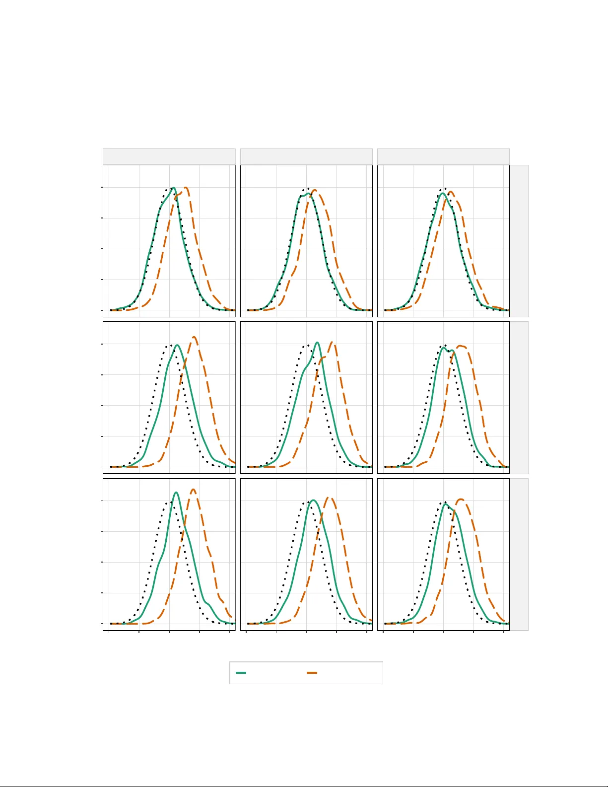
T riple/Double-Debiased Lasso ∗ Denis Chetv erik o v 1 , Jesp er R.-V. Sørensen 2,4 , and Aleh Tsyvinski 3 1 University of California, L os A ngeles 2 University of Cop enhagen 3 Y ale University 4 A arhus Center for Ec onometrics (ACE) Marc h 23, 2026 Abstract In this pap er, w e prop ose a triple (or double-debiased) Lasso estimator for infer- ence on a l ow-dimensional parameter in high-dimensi onal linear regression models. The estimator is based on a momen t function that satisﬁes not only ﬁrst- but also second- order Neyman orthogonality conditions, thereb y eliminating both the leading bias and the second-order bias induced b y regularization. W e deriv e an asymptotic linear rep- resen tation for the proposed estimator and show that its remainder terms are never larger and are often smaller in order than those in the corresp onding asymptotic linear represen tation for the standard double Lasso estimator. Because of this impro v ement, the triple Lasso estimator often yields more accurate ﬁnite-sample inference and conﬁ- dence interv als with better co verage . Mon te Carlo simul ations conﬁrm these gains. In addition, we provide a general recursiv e formula for constructing higher-order Neyman orthogonal momen t functions in Z-estimation problems, which underlies the prop osed estimator as a sp ecial case. 1 In tro duction Inference on a lo w-dimensional target parameter in the presence of many controls has b e- come a central problem in econometrics b ecause making a condi tional exogeneit y assumpti on ∗ W e thank Jin Hahn, Whitney New ey , and Andres San tos for their helpful commen ts. Sørensen is grateful for rese arch support from the Aarhus Cen ter for Econometrics (ACE) funded b y the Danish National Research F oundation gran t n um b er DNRF186. 1 plausible in empirical applications often requires using a rich set of cov ariates ( Belloni et al. , 2017 ). In such settings, in addition to the target parameter, w e also hav e a high-dimensional n uisance parameter that has to b e estimated via mac hine learning methods suc h as the Lasso estimator. Unfortunately , regularization underlying these mac hine learning metho ds gener- ates non-regular ﬁrst-stage bias that t ypically in v alidates naiv e plug-in inference pro cedures for the target parameter. A ma jor insight of the double/debiased machin e learning litera- ture is that this problem can often b e ov ercome by replacing the original moment equation with the one based on a moment function whose ﬁrst deriv ativ e with resp ect to the nuisance parameter v anishes at the true parameter v alues (ﬁrst-order Neyman orthogonalit y condi- tion), so that suﬃ ciently accurate regularized estimators of the nuisan ce parameter matter only through second-order remainder terms and the target parameter can b e estimated at the usual 1 / √ n rate ( Chernozhuk o v et al. , 2015 ). In this pap er we sho w tha t, in the high- dimensional linear regression mo del, one can go one step further and construct an estimator that remov es not only the ﬁrst-order eﬀect of nui sance parameter estimation but also the second-order eﬀect. Because of the steps in the construction of our estimator, we refer to it as a triple L asso estimator, or, equiv alen tly , a double-debiase d L asso estimator. Our starting p oin t is the standard high-dimensional linear regression mo del in whic h the outcome is regressed on a scalar treatmen t v ariable of in terest and a p oten tially high- dimensional v ector of con trols. In this mo del, the con v entional double Lasso estimator ( Bel- loni et al. , 2014 ) is based on a momen t function that satisﬁes the ﬁrst-order Neyman or- thogonalit y condition and is often remark ably successful ev en when the underlying Lasso estimators are far from b eing √ n -consisten t. Ho wev er, the momen t function b ehind the double Lasso estimator do es not satisfy the se c ond-or der Neyman orthogonalit y condition, and this means that the double Lasso estimator may p erform p o orly if second-order remain- der terms are large enough to matter in empirically relev an t samples, whic h happ ens when the ﬁrst-stage Lasso estimators con v erge rather slo wly . Our ﬁrst main con tribution is th us to construct a momen t function that satisﬁes not only the ﬁrst-order but also the second-order Neyman orthogonalit y condition. Our momen t function is obtained from the double Lasso momen t function by subtractin g a carefully c hosen quadratic correction term, weigh ted b y the inv erse Gram matrix of the con trols, so that the second-order bias term is cancelled by construction. In turn, our second main con tribution is to prop ose the triple Lasso estimator that solv es a moment condition based on this momen t function, with all underlying nuisance parameters b eing estimated b y the Lasso-type metho ds. W e deriv e an asymptotic lin ear represen tation for our triple Lasso estimator and compare its remainder terms with those of the usual double Lasso estimator. W e show that whenever the double Lasso estimator is already asymptotically normal, the remainder terms for the 2 triple Lasso estimator are never lar ger and are often strictly smaller in order than the cor- resp onding terms for the double Lasso estimator. As a result, the distribution of the triple Lasso estimator is often closer to the properly cen tered normal distribution than that of the double Lasso estimator. Moreo ver, in the sp ecial case of exact sparsity and consisten t Lasso screening, the triple Lasso estimator can remain asymptotically normal along sequences of data-generating pro cesses for which the double Lasso estimator fails to b e asymptotically normal. Our Monte Carlo simulations conﬁrm that the implications of the asymptotic theory remain relev ant in empirically meaningful ﬁnite-sample settings. Across designs that v ary the sample size, the correlation structure of the con trols, and the sparsit y of the n uisance parameters, although the v ariance of the triple Lasso estimator is t ypically somewhat larger than that of the double Lasso es timator, the former estimator often has substan tially smaller squared bi as and the mean squared error, esp ecially in the harder designs. More importantly , ho wev er, the triple Lasso estimator often leads to more precise inference. F or example, in one of the designs, the empirical co v erage of nominal 95% conﬁdence in terv als rises from about 67% under the double Lasso estimator to about 92% under the triple Lasso estimator. This happ ens despite the fact that the triple Lasso conﬁdence interv als are only sligh tly longer on a vera ge. As our third main contribution, w e extend the construction of the second-order Neyman orthogonal momen t functio n to a general Z-est imation problem. In fact, we provide a gen- eral recursiv e form ula that can be used to construct momen t functions in the Z-estimation problem that satisfy the Neyman orthogonalit y condition to any desired order. W e fur- ther illustrate this construction in an M-estimation problem with a single-index structure, deliv ering the results for the high-dimensional linear regression mo del as a sp ecial case. Our paper is related to severa l strands of the literature. First, it builds directly on the foundational w ork on double/debiased Lasso and post-selection inference in high-dimensional linear regression mo dels, including Belloni et al. ( 2014 ), Ja v anmard and Mon tanari ( 2014 ), v an de Geer et al. ( 2014 ), and Zhang and Zhang ( 2014 ), all of which established that v alid inference on lo w-dimensional comp onent s is p ossible after reg ularization when the momen t function is appropriately debiased. Closely related is the double machine learning literature of Chernozhuk o v et al. ( 2015 ) and Chernozhuk o v et al. ( 2018 ), from which w e adopt the em- phasis on orthogonal moment functions, while extending that persp ective from ﬁrst-order to higher-order orthogonalit y . An alternative approac h to inference in high-dimensional linea r regression models is dev elop ed b y Ar mstrong et al. ( 2020 ), who propose explicitly accoun ting for the bias induced b y regularization rather th an elimina ting it through orthogonalization; an adv an tage of this approac h is that it achiev es v alidity under w eaker structural conditions, 3 although it requires the researcher to specify a b ound on the mag nitude of the nuisance co- eﬃcien ts. Second, our pap er is connected to the broader literature on appro ximately sparse high-dimensional mo dels, including Belloni and Chernozh uko v ( 2011 ), Belloni et al. ( 2012 ), and v an de Geer ( 2016 ), from whic h we b orro w tech nical to ols, in particular the conv ergence rates for Lasso estimators in linear regression mo dels and for node-wise Lasso estimators of in v erse Gram matrices. Third, our paper is rel ated to the emergi ng literature on higher-order orthogonalit y , including Mack ey et al. ( 2018 ) and Bonhomme et al. ( 2024 ). In particular, Mac key et al. ( 2018 ) construct higher-order Neyman orthogonal moment functions for the partially linear mo del under non -Gaussian ﬁrst-stage errors, while Bonhomme et al. ( 2024 ) dev elop a general algorithm for constructing higher-order Neyman orthogonal moment func- tions in likelihoo d-based mo dels. These results are not direct ly app licable in our setting, as w e fo cus on regression-based esti mation rather than lik elihoo d models and do not restrict the distribution of noise. Also, our results do not con tradict the negative result in Mack ey et al. ( 2018 ) on the existence of higher-order Neyman orthogonal momen t functions in the par- tially linear mo del with Gaussian ﬁrst-stage errors, b ecause our moment function dep ends not only on a vecto r of observ able random v ariables but also on an indep enden t cop y of this v ector, and, moreov er, our orthogonality requiremen t is form ulated in terms of ordinary deriv atives rather than the stronger functional-deriv ativ e notion studied there, reﬂecting the parametric nature of our regression mo del. Finally , our pap er is also related to earlier w ork on higher-order inﬂuence functions and U-statistic-based estimators in semiparametric and nonparametric mo dels, including Robins et al. ( 2008 ), Robins et al. ( 2017 ), Newey and Robins ( 2018 ), and Liu et al. ( 2023 ), whic h develo p higher-order expansions of functionals and corresp onding estimators that balance bias and v ariance in settings where ﬁrst-order in- ﬂuence function metho ds are insuﬃcien t. This literature shows that higher-order corrections can be used to relax smo othness requ irements and/or impro v e rates in semiparametric and nonparametric mo dels. The rest of the pap er is organized as follo ws. Section 2 in troduces the triple Lasso momen t function and the corresponding estimator in the high-dimensi onal li near regression mo del, prov es second-order Neyman orthogonalit y of the prop osed momen t function, and deriv es the asymptotic linear represen tation and asymptotic normalit y result for the triple Lasso estimator. Section 3 develops the general recursiv e form ula for constructing higher- order Neyman orthogonal momen t functi ons for the Z-estim ation problem and applies it to M-estimators with a single-index structure, thereby showing that the logic b ehind the triple Lasso estimator is a part of a broader higher-order orthogonalization principle. Section 4 rep orts Mon te Carlo results showing that the triple Lasso estimator can substan tially reduce bias and deliv er more reliable inference in comparison with the double L asso estimator under 4 certain data-generating pro cesses. Notation F or an y p ∈ N , we denote [ p ] : = { 1 , . . . , p } and 0 p : = (0 , . . . , 0) ⊤ ∈ R p . Also, we let 0 p × p and I p b e the zero and identit y matrices in R p × p , resp ectiv ely . In addition, for an y ﬁnite set of p ositiv e integ ers I , w e use E I [ f ( X i )] to denote the a v erage v alue of f ( X i ) as i v aries ov er I , namely E I [ f ( X i )] = | I | − 1 P i ∈ I f ( X i ). F or n umbers a n and b n , n ∈ N , we write a n ≲ b n if there exists a constant C > 0 such that | a n | ≤ C | b n | for all n ∈ N . F or random v ariables V n and R n , n ∈ N , we write V n ≲ P R n if V n = Y n R n for some Y n = O P (1). Finally , for an y matrix A = ( A j,k ) p j,k =1 , w e denote ∥ A ∥ max : = max 1 ≤ j,k ≤ p | A j,k | and ∥ A ∥ ∞ : = max 1 ≤ i ≤ p P p j =1 | A j,k | . 2 T riple Lasso Estimator In this section, we prop ose a moment function for the high-dimensional linear regression mo del that satisﬁes the second-order Neyman orthogonalit y condition and int ro duce the corresp onding triple Lasso estimator. In addition, we deriv e the √ n -consistency and asymp- totic normality result for our triple Lasso estimator and compare the remainder terms of the corresp onding asymptotic linear represen tation to those underlying the asymptotic linear represen tation for the double Lasso estimator. 2.1 Mo del, Second-Order Neyman Orthogonality , and Estimation Consider the linear regression mo del Y = D β 0 + X ⊤ θ 0 + ε, E[ ε | D , X ] = 0 , (1) where Y ∈ R is the outcome, D ∈ R is a regressor of in terest, X = ( X 1 , . . . , X p ) ⊤ ∈ R p is a vector of con trols, β 0 ∈ R is the parameter of in terest, and θ 0 = ( θ 0 , 1 , . . . , θ 0 ,p ) ⊤ ∈ R p is a vect or of n uisance parameters. Let ( X i , D i , Y i ), i = 1 , . . . , n , b e a random sample from the distribution of ( X , D, Y ), where we denote X i = ( X i, 1 , . . . , X i,p ) ⊤ for all i ∈ [ n ]. In this pap er, we primarily fo cus on the high-dimensional setting in whic h the n um b er of con trols p ma y b e comparable to or larger than th e sample size n . A con v en tional w ay to estimate β 0 in model ( 1 ) when p is large is via the double Lasso 5 estimator. 1 T o descr ib e it, let the pr o jection of D on X b e D = X ⊤ γ 0 + ν , E[ ν X ] = 0 p , (2) where γ 0 = ( γ 0 , 1 , . . . , γ 0 ,p ) ⊤ ∈ R p is a v ector of parameters, and let the reduced-form regres- sion of Y on X b e Y = X ⊤ ϕ 0 + e, E[ e X ] = 0 p , (3) where ϕ 0 = ( ϕ 0 , 1 , . . . , ϕ 0 ,p ) ⊤ : = θ 0 + β 0 γ 0 and e : = ε + β 0 ν . One v ersion of the double Lasso estimator is constructed as follo ws. First, estimate ϕ 0 b y running the Lasso regression of Y on X , yielding b ϕ . Second, estimate γ 0 b y running the Lasso regression of D on X , yielding b γ . Third, estimate β 0 b y running the OLS regression of Y − X ⊤ b ϕ on D − X ⊤ b γ , yielding the double Lasso estimator b β DL . Under certain conditions, the double Lasso estimator is √ n - consisten t and asymptotically normal, despite the fact that the underlying Lasso estimators b ϕ and b γ are not √ n -consisten t. T o un derstand why this happens, introduce the momen t function ψ DL : R × R p × R p b y ψ DL ( β , γ , ϕ ) : = E[( Y − X ⊤ ϕ − β ( D − X ⊤ γ ))( D − X ⊤ γ )] and observ e that the true v alue β 0 satisﬁes the momen t equation ψ DL ( β , γ 0 , ϕ 0 ) = 0 . (4) The double Lasso estimator b β DL solv es an empirical analogue of this equation obtained b y replacing the population exp ectation with the empirical exp ectation and the true v alues γ 0 and ϕ 0 with their estimators b γ and b ϕ . The k ey fact underlying the √ n -consistency and asymptotic normality of the double Lasso estimator is that there is no ﬁrst-order eﬀect of replacing γ 0 and ϕ 0 b y b γ and b ϕ on the moment function ψ DL : ∂ ψ DL ( β 0 , γ 0 , ϕ 0 ) ∂ γ = 0 p and ∂ ψ DL ( β 0 , γ 0 , ϕ 0 ) ∂ ϕ = 0 p . (5) Indeed, pro vided that the estimators b γ and b ϕ are suﬃcien tly precise so that the second- order eﬀects are asymptotically negligible, condition ( 5 ) ensures that the estimator b β DL is asymptotically equiv alent to the infeasible estimator e β DL obtained by solving the empirical analogue of ( 4 ) in which only the p opulation exp ectation is replaced b y the empirical ex- p ectation. The lat ter estimator is in turn √ n -consisten t and asymptotically normal by th e 1 V arious v ersions of the double/debiased Lasso estimator app eared in Belloni et al. ( 2014 ), Jav anmard and Mon tanari ( 2014 ), v an de Geer et al. ( 2014 ), and Zhang and Zhang ( 2014 ). 6 classic M -estimation theory . Because of ( 5 ), the moment function ψ DL is said to satisfy the (ﬁrst-order) Neyman ortho gonality condition. T o express this condition more compactly , let η : = ( γ ⊤ , ϕ ⊤ ) ⊤ and η 0 : = ( γ ⊤ 0 , ϕ ⊤ 0 ) ⊤ . Then ( 5 ) can be written equiv alen tly as ∂ ψ DL ( β 0 , η 0 ) ∂ η = 0 2 p . Similarly , one can deﬁne the second-order Neyman orthogonality . F ollo wing Mack ey et al. ( 2018 ) and Bonhomme et al. ( 2024 ), we sa y that a moment function ψ : R × R q → R satisﬁes the se c ond-or der Neyman ortho gonality condition if ∂ ψ ( β 0 , η 0 ) ∂ η = 0 q and ∂ 2 ψ ( β 0 , η 0 ) ∂ η ∂ η ⊤ = 0 q × q , where η 0 ∈ R q is a vector of n uisance parameters. Intuitiv ely , using estimators based on momen t functions satisfyin g the second-order Neyman orthogonalit y condition is beneﬁcial b ecause such momen t functions eliminate not only the ﬁrst-order eﬀects of replacing the true v alues of the n uisance parameters by the corresp onding estimators but also the second- order eﬀects. Unfortunately , how ev er, the momen t function ψ DL underlying the double Lasso estimator do es not ha ve this prop erty . Indeed, it is straigh tforw ard to v erify that ∂ 2 ψ DL ( β 0 , γ 0 , ϕ 0 ) ∂ γ ∂ ϕ = E[ X X ⊤ ]  = 0 p × p . It therefore follo ws that con v ergence of the double Lasso estimator to the prop erly cen tered normal distribution may fail or b e slow if the Lasso estimators b γ and b ϕ are not suﬃcien tly precise and the second-order eﬀects are non-negligible. Motiv ated by this observ ation, we prop ose a no v el moment function for estimating β 0 in mo del ( 1 ) that satisﬁes not only the ﬁrst-order Neyman orthogonality condition but also the second-order Neyman orthogonalit y condition. W e then deﬁne a triple L asso estimator that solv es an empirical analogue of the moment condition implied by this function and derive its asymptotic prop erties. In order to in tro duce our momen t function, let Σ 0 : = E[ X X ⊤ ] denote the p opulation Gram matrix of the con trols X , and let Θ 0 : = Σ − 1 0 denote its inv erse. Deﬁne the function ψ ADJ : R × R p × R p × R p × p b y ψ ADJ ( β , γ , ϕ , Θ ) : = E[( Y − X ⊤ ϕ − β ( D − X ⊤ γ )) X ⊤ Θ ˜ X ( ˜ D − ˜ X ⊤ γ )] , 7 where ( ˜ X , ˜ D ) is a cop y of ( X , D ) that is indep enden t of ( X , D , Y ). Our mo ment function ψ T L : R × R 2 p + p 2 → R for estimating β 0 in mo del ( 1 ) is then deﬁned as ψ T L ( β , η ) : = ψ DL ( β , γ , ϕ ) − ψ ADJ ( β , γ , ϕ , Θ ) , η : = ( γ ⊤ , ϕ ⊤ , vec( Θ ) ⊤ ) ⊤ . (6) In the follo wing lemma, we sho w that the true v alue β 0 solv es the moment equation ψ T L ( β , η 0 ) = 0 , (7) where η 0 : = ( γ ⊤ 0 , ϕ ⊤ 0 , vec( Θ 0 ) ⊤ ) ⊤ and that the momen t function ψ T L satisﬁes the second- order Neyman orthogonalit y condition. The pro of of this lemma can b e found in the Ap- p endix. Lemma 2.1. As long as the moments E[ Y 2 ] , E[ D 2 ] , and E[ ∥ X ∥ 2 2 ] ar e ﬁnite and the matrix E[ X X ⊤ ] is invertible, we have ψ T L ( β 0 , η 0 ) = 0 and al l ﬁrst- and se c ond-or der derivatives of the function η 7→ ψ T L ( β 0 , η ) at η = η 0 ar e zer o. Remark 2.1. It is in teresting to compare Lemma 2.1 with a negativ e result on the existence of higher -order Neyman orthogonal momen t functi ons in Mack ey et al. ( 2018 ), abbreviated as MSZ b elo w. They consider the closely related partially linear mo del Y = D β 0 + f 0 ( X ) + ε, E[ ε | D , X ] = 0 , D = g 0 ( X ) + ν , E[ ν | X ] = 0 , and sho w that if the conditional distribution of ν given X is Gaussian, then an y t wice diﬀeren tiable score function m that is second-order Neyman orthogonal with resp ect to f 0 and g 0 m ust satisfy ∂ E[ m ( Z , β 0 , η 0 )] ∂ β = 0 , where Z : = ( X , D , Y ) and η 0 includes the n uisance functions f 0 and g 0 . The latter in turn essentially rules out √ n -consisten t estimation of β 0 based on the moment condition E[ m ( Z , β 0 , η 0 )] = 0. In contrast, for our high-dimensional linear regression mo del, w e do ha ve ∂ ψ T L ( β 0 , η 0 ) ∂ β = − E[( D − X ⊤ γ 0 ) 2 ]  = 0 . T o resolv e this apparen t contradi ction, w e make t wo observ ations. First, the score functio n underlying our moment function ψ T L dep ends not only on ( X , D , Y ) but also on an inde- p enden t cop y ( ˜ X , ˜ D ) of ( X , D ). Second, our second-order Neyman orthogonalit y condition is weak er than that imp osed in MSZ: w e only require certain or dinary deriv atives to v an- 8 ish, whereas MSZ require certain functional deriv atives to v anish, reﬂecting the parametric nature of our mo del. Remark 2.2. It is also in teresting to compare the momen t function ψ T L with what can b e obtained from the algorithm of Bonhomme et al. ( 2024 ), abbreviated as BJW below. Since their algorithm applies only to likeli ho o d mo dels and cannot, in general, b e used directly in regression settings, we em b ed our mo del ( 1 )-( 2 ) into a lik elihoo d framework b y imp osing additional distributional assumptions on the vector of controls X and the disturbances ( ε, ν ). In particular, for the purposes of this comparison, w e assume that the distribution of X is kno wn and that the conditional distribution of ( ε, ν ) giv en X is standard normal. Under these assumptions, our regression mo del reduces to a lik eliho o d mo del, and applying the BJW algorithm yields the momen t function ψ B K W : R × R 2 p → R deﬁned b y ψ B K W ( β , η ) : = E[(1 − E[ m ⊤ ](E[ mm ⊤ ]) − 1 m )( Y − D β − X ⊤ θ )( D − X ⊤ γ )] , η : = ( γ ⊤ , θ ⊤ ) ⊤ , where m : = v ech( X X ⊤ ), where the operator v ech stacks the elements of the low er triangular part, including the diagonal, of the matrix into a vector. By construction, this momen t function satisﬁes the second-order Neyman orthogonalit y condition under these distributional assumptions. How ev er, if we relax these assumptions and only main tain E[ ε | X ] = 0 and E[ ν X ] = 0 p as in model ( 1 )-( 2 ), then the deriv ativ e ∂ ψ B K W ( β 0 , η 0 ) /∂ θ need not v anish, so that ψ B K W ma y fail to satisfy even the ﬁrst-order Neyman orthogonalit y condition. On the other hand, and p erhaps more interestin gly , if we strengthen the assump tions to E[ ε | X ] = 0 and E[ ν | X ] = 0, then the moment function ψ B K W satisﬁes the second-order Neyman orthogonalit y condition not only with resp ect to η = ( γ ⊤ , θ ⊤ ) ⊤ , but also with resp ect to the extended v ector ˜ η : = ( γ ⊤ , θ ⊤ , E[ m ⊤ ] , vec h(E[ mm ⊤ ]) ⊤ ) ⊤ , whic h is a desir able feature. Ho wev er, using this momen t function in practice requires esti- mating and inv erting the ( p ( p + 1) / 2) × ( p ( p + 1) / 2) matrix E[ mm ⊤ ], whic h ma y be hard and may require non-standard conditions. In con trast, using our momen t function ψ T L only requires estimating and in verti ng the m uc h smaller p × p matrix E[ X X ⊤ ]. W e next deﬁne the triple Lasso estimator as a solution to an empirical analogue of equation ( 7 ), where γ 0 and ϕ 0 are replaced by the corresp onding Lasso estimators and Θ 0 is replaced b y the no de-wise Lasso estimator. F or the r easons that will b ecome clear shortly , w e in fact use ro w-sparsiﬁed v ersion of the node-wise Lasso estimator of Θ 0 . In addition, since it is useful for the asymptotic normality result, we also com bine the estimator with cross- 9 ﬁtting, whic h is standard in the literature on double mac hine learning; see Chernozh uk ov et al. ( 2018 ). T o formally describ e the resulting estimator, split at random the full sample into K subsamples of appro ximately the same size for some small K and let I (1) , . . . , I ( K ) be the sets of indices from 1 to n corresp onding to the observ ations in these subsamples. Also, for eac h k ∈ [ K ], let I ( − k ) : = [ n ] \ I ( k ). Then for each k ∈ [ K ], let b γ k = ( b γ k, 1 , . . . , b γ k,p ) ⊤ , b ϕ k = ( b ϕ k, 1 , . . . , b ϕ k,p ) ⊤ , and e Θ k = ( e Θ k,j,l ) j,l ∈ [ p ] b e the Lasso estimator of γ 0 , the Lasso estimator of ϕ 0 , and the no de-wise Lasso estimator of Θ 0 , resp ectiv ely , all deﬁned on the subsample of observ ations with indices in I ( − k ). Here, w e use the row-wi se versi on of the no de-wise Lasso estimator. Sp eciﬁcally , to deﬁne the ﬁrst ro w e Θ k, 1 of the matrix e Θ k , we run the Lasso regression of X 1 on X − 1 : = ( X 2 , . . . , X p ) ⊤ and obtain the v ector of slop e coeﬃcien ts, sa y b ψ 1 . Then we set b σ 2 1 : = E I ( − k ) [ X i, 1 ( X i, 1 − X ⊤ i, − 1 b ψ 1 )] and e Θ k, 1 : = (1 , − b ψ ⊤ 1 ) / b σ 2 1 , where X i, − 1 : = ( X i, 2 , . . . , X i,p ) ⊤ . All other rows of e Θ k are deﬁned analogously . Next, let b T k, 0 : = { j = 1 , . . . , p : b γ k,j  = 0 } b e the set of indices from 1 to p corresp onding to the non-zero comp onen ts of the vect or b γ k and let b Θ k b e the R p × p matrix obtained from e Θ k b y setting to zero all its rows whose indices are not in b T k : = b T k, 0 ∪ b T k, 1 , where b T k, 1 is an additional set of indices corresp onding to the ext ra v ariables that the researc her migh t wan t to use as we discuss b elo w. Throughout most of the pap er, w e assume that b T k, 1 = ∅ . T o deﬁne b β k , w e no w solve an empiri cal version of the equation ( 7 ) on I k for β , namely w e set b β k : = E I ( k ) [( Y i − X ⊤ i b ϕ k )( D i − X ⊤ i b γ k )] − E I ( k ) [( Y i − X ⊤ i b ϕ k ) X ⊤ i ] b Θ k E I ( k ) [ X i ( D i − X ⊤ i b γ k )] E I ( k ) [( D i − X ⊤ i b γ k ) 2 ] − E I ( k ) [( D i − X ⊤ i b γ k ) X ⊤ i ] b Θ k E I ( k ) [ X i ( D i − X ⊤ i b γ k )] . Finally , we aggregate the subsample estimators b β k to obtain the triple (or double-debiased) Lasso estimator: b β T L : = 1 K K X k =1 b β k . In the next subsection, we will deriv e the asymptotic theory for the triple Lasso estimator b β T L and compare it with that for the d ouble Lasso estimator b β DL . Remark 2.3. W e now explain why w e use sparsiﬁed ver sions b Θ k of the no de-wise Lasso estimators e Θ k of Θ 0 . Consider an idealized case where E[ X X ⊤ ] is equal to the iden tit y matrix I p and this fact is known to the researcher. In thi s case, w e could replace b Θ k in the expression for b β k ab o v e b y I p . Doing so would lead to the follo wing term in the n umerator of b β k : E I k [( Y i − X ⊤ i b ϕ k ) X ⊤ i ]E I k [ X i ( D i − X ⊤ i b γ k )] . Substituting here the expressions for D i and Y i from ( 2 ) and ( 3 ), resp ectiv ely , yields terms of 10 the form E I k [ ε i X ⊤ i ]E I k [ X i ν i ]. In turn, such terms are diﬃcult to con trol when p is comparable to or larger than n . In particular, it is straigh tforward to verify that they are typi cally of order √ p/n in probabilit y , whic h is to o large for our purp oses. By in troducing sparsiﬁcation, w e substan tially reduce the v ariance of these terms at the exp ense of in tro ducing some bias. Remark 2.4. Although w e fo cus on Lasso-type metho ds throughout this section, whic h lead to the triple Lasso esti mator, the moment function ψ T L can in principle be com bined with other machine learning metho ds suitable for estimating the n uisance parameters γ 0 , ϕ 0 , and Θ 0 . F or instance, γ 0 and ϕ 0 can b e estimated using the Dantzig selector, while Θ 0 can b e estimated via a Dan tzig-t yp e pro cedure as discussed, for example, in Jav anmard and Mon tanari ( 2014 ). In fact, the asymptotic theory d eveloped in the n ext subsect ion is agnostic to the speciﬁc c hoice of estimators, pro vided they achiev e the required leve l of precision as sp eciﬁed in our assumptions. 2.2 Asymptotic Theory In this subsection, we establish the √ n -consistency and asymptotic normalit y result for the triple Lasso estimator b β T L . T o this end, w e imp ose several regularit y conditions. Th ese conditions con trol the moments of the disturbances ( ε, ν ), the sample splitting scheme used in the construction of the estimator, the b eha vior of the Lasso estimators app earing in the algorithm, and the sparsit y of the model. Assumption 2.1. (1) The r andom variables ε and ν have b ounde d fourth moments: E[ | ε | 4 ] ≲ 1 and E[ | ν | 4 ] ≲ 1 ; (2) the se c ond moment of ν is b ounde d b elow fr om zer o: (E[ ν 2 ]) − 1 ≲ 1 . Assumption 2.2. Ther e exists a c onstant C ∈ (0 , ∞ ) such that E[ ε 2 | X ] ≤ C , E[ ν 2 | X ] ≤ C , and ∥ X ∥ ∞ ≤ C almost sur ely. Assumption 2.3. F or al l k ∈ [ K ] , the subsample I ( k ) c ontains a non-vanishing fr action of the ful l sample: | I ( k ) | − 1 ≲ n − 1 . Assumptions 2.1 – 2. 3 imp ose basic moment and regularit y conditions on the disturbances, regressors, and the sample splitting scheme. Assumption 2.1 requires the disturbances ε and ν to hav e b ounded fourth moments and the v ariance of ν to b e b ounded aw a y from zero. The latter serves as an iden tiﬁcation condition ensuring that the leading term in the asymptotic expansion of the triple Lasso estimator has ﬁnite v ariance. Assumption 2.2 imp oses mild b oundedness conditions on the conditional second moments of ε and ν and requires the regressors to b e uniformly b ounded. These condit ions simplify the deriv ations but w e note that our results can b e extended to allo w for un b ounded con trols. W e w ork with 11 b ounded con trols to a v oid tec hnicalities and to k eep the argumen ts transparent. Finally , Assumption 2.3 formalizes the requiremen t that the subsamples used in cross-ﬁtting contain a non-v anishing fraction of the observ ations in the full sample. Since the num b er of folds K is ﬁxed, this condition guarant ees that the n um b er of observ ations in eac h subsample is of order n . Assumption 2.4. Ther e ar e non-r andom se quenc es s γ : = s γ ,n and s θ : = s θ ,n of inte gers in [1 , ∞ ) and non-r andom se quenc es ¯ γ 0 : = ¯ γ 0 ,n and ¯ θ 0 : = ¯ θ 0 ,n of ve ctors in R p such that: (1) the ve ctors ¯ γ 0 and ¯ θ 0 ar e sp arse: ∥ ¯ γ 0 ∥ 0 ≤ s γ and ∥ ¯ θ 0 ∥ 0 ≤ s θ ; (2) the ve ctors ¯ γ 0 and ¯ θ 0 pr ovide go o d appr oximation to the p ar ameter ve ctors γ 0 and θ 0 : ∥ γ 0 − ¯ γ 0 ∥ 2 2 ≲ s γ /n , ∥ γ 0 − ¯ γ 0 ∥ 2 1 ≲ s 2 γ /n , E[ X ⊤ ( γ 0 − ¯ γ 0 ) | 2 ] ≲ s γ /n , ∥ θ 0 − ¯ θ 0 ∥ 2 2 ≲ s θ /n , ∥ θ 0 − ¯ θ 0 ∥ 2 1 ≲ s 2 θ /n , and E[ X ⊤ ( θ 0 − ¯ θ 0 ) | 2 ] ≲ s θ /n ; (3) for al l k ∈ [ K ] , the estimators b γ k and b ϕ k ar e suﬃciently ac cur ate for ¯ γ 0 and ¯ ϕ 0 : = ¯ θ 0 + β 0 ¯ γ 0 : ∥ b γ k − ¯ γ 0 ∥ 2 2 ≲ P s γ log p/n , ∥ b γ k − ¯ γ 0 ∥ 2 1 ≲ P s 2 γ log p/n , ∥ b ϕ k − ¯ ϕ 0 ∥ 2 2 ≲ P s ϕ log p/n , and ∥ b ϕ k − ¯ ϕ 0 ∥ 2 1 ≲ P s 2 ϕ log p/n , wher e we denote d s ϕ : = s θ + s γ ; (4) for al l k ∈ [ K ] , the estimators b γ k and b ϕ k ar e suﬃciently sp arse: ∥ b γ k ∥ 0 ≲ P s γ and ∥ b ϕ k ∥ 0 ≲ P s ϕ ; (5) the matrix E[ X X ⊤ ] satisﬁes a sp arse eigenvalue c ondition: λ max ,s ϕ ℓ n (E[ X X ⊤ ]) ≲ 1 for some ℓ n → ∞ as n → ∞ ; (6) for al l k ∈ [ K ] , the sets b T k ar e suﬃciently sp arse: | b T k | ≲ P s γ . Assumption 2.4 imp oses appro ximate sparsity and regularity conditions th at are standard in the analysis of Lasso estimators. Parts 1 and 2 require that the parameters γ 0 and θ 0 admit sparse appro ximations ¯ γ 0 and ¯ θ 0 with sparsit y indices s γ and s θ and formalize the qualit y of these appro ximations b y requiring the appro ximation errors to be small in b oth ℓ 2 and ℓ 1 norms as w ell as in the prediction norm induced b y the con trols X . Comparable conditions app ear, for example, in Belloni et al. ( 2014 ) and Chernozh uko v et al. ( 2015 ). Parts 3 and 4 imp ose the usual rate and sparsity prop erties of the Lasso estimators b γ k and b ϕ k obtained in the auxiliary regressions. These conditions are satisﬁed under typically used assumptions on the design matrix, as explained for example in Belloni and Chernozh uko v ( 2011 ), and ensure that the preliminary estimators are suﬃcien tly accurate for the sparse appro ximations ¯ γ 0 and ¯ ϕ 0 . P art 5 imp oses a classical sparse eigen v alue condition on the p opulation Gram matrix E[ X X ⊤ ], meaning that sparse subsets of the regressors are not excessiv ely collinear. Finally , Part 6 requires the sets b T k used in the construction of the triple Lasso estimator to b e suﬃcien tly sparse. In ligh t of Part 4 , this condition holds trivially if b T k, 1 = ∅ . 12 Assumption 2.5. F or al l k ∈ [ K ] , the no de-wise L asso estimators e Θ k ar e such that: (1) ∥ e Θ k E I ( − k ) [ X i X ⊤ i ] − I p ∥ 2 max ≲ P log p/n ; (2) ∥ e Θ k ∥ ∞ ≲ P 1 . Assumption 2.6. We have (1) √ s γ s ϕ log p/n = o (1) ; (2) s 3 γ s ϕ (log p ) 3 /n 2 = o (1) . Assumption 2.5 imp oses regularity conditions in terms of con v ergence rates on the no de- wise Lasso estimators used to appro ximate the inv erse Gram matrix Θ 0 = E[ X X ⊤ ] − 1 . These con v ergence rates are w ell-established in the literature on estimation of inv erse Gram matrices; see, for example, v an de Geer ( 2016 ). Part 1 requires that the estimators e Θ k pro vide suﬃcien tly accurate appro ximations to the inv erse of the empirical Gram matrix computed on the subsample I ( − k ). P art 2 ensures that eac h row of the estimator e Θ k remains b ounded in the ℓ 1 norm. Assumption 2.6 restricts the growth of the sparsit y indices relativ e to the sample size. In particular, it requires that the sparsit y lev els s γ and s ϕ do not gro w to o quickly compared to n and log p . Note also that Assumption 2.6 is weak er than the corresp onding conditions used to deriv e the √ n -consistency and asymptotic normalit y result for the double Lasso estimator; see Belloni et al. ( 2014 ) for the case of the original double Lasso estimator and Chernozh uk ov et al. ( 2018 ) for the case of the double Lasso estimator com bined with cross-ﬁtting. W e are no w ready to establish the main result of this pap er, whic h sho ws that the triple Lasso estimator b β T L is √ n -consisten t and asymptotically normal under our assumptions. The pro of of this theorem can b e found in the App endix. Theorem 2.1. Under Assumptions 2.1 – 2.6 , √ n ( b β T L − β 0 ) = 1 √ n n X i =1 ε i ν i E[ ν 2 ] + O P ( R 1 ) + O P ( R 2 ) + O P ( R 3 ) , (8) wher e R 1 : = s 1 / 4 γ p s ϕ log p √ n , R 2 : = s 3 / 2 γ √ s ϕ (log p ) 3 / 2 n , (9) R 3 : = p s ϕ log p   1 K K X k =1 ∥ ¯ γ 0 − ¯ γ 0 , b T k ∥ 2 + p E[ | X ⊤ ( γ 0 − ¯ γ 0 ) | 2 ] + ∥ γ 0 − ¯ γ 0 ∥ 2   . (10) Ther efor e, √ n ( b β T L − β 0 ) → d N (0 , V ) , V : = E[( εν ) 2 ] (E[ ν 2 ]) 2 , as long as R 3 = o P (1) . 13 The result in Theorem 2.1 for the triple Lasso estimator can b e compared with the corresp onding result for the double Lasso estimator. In particular, it follows from the pro of of Theorem 2.1 that the cross-ﬁtted double Lasso estimator b β DL satisﬁes √ n ( b β DL − β 0 ) = 1 √ n n X i =1 ε i ν i E[ ν 2 ] + O P ( R 4 ) , R 4 : = √ s γ s ϕ log p √ n , (11) whic h is essen tially a well-kno wn result; e.g., see Chernozh uk o v et al. ( 2018 ). Both estimators are therefore √ n -consisten t and prop erly cen tered asymptotically normal if the corresp ond- ing remainder terms in asymptotic linear represen tations ( 8 ) and ( 11 ) are asymptotically v anishing. In turn, to compare the remainder terms, supp ose ﬁrst that R 4 = o (1) so that the double Lasso estimator is √ n -consisten t and asymptotically normal. W e claim that then the remainder terms R 1 , R 2 , and R 3 for the triple Lasso estimator are always at most of the same or der as the remainder term R 4 for the double Lasso estimator and often of smal ler or der . Indeed, R 1 R 4 = 1 s 1 / 4 γ √ log p = o (1) whenev er either p → ∞ or s γ → ∞ , and R 2 R 4 = s γ √ log p √ n ≤ R 4 = o (1) since s ϕ ≥ s γ b y the deﬁnition of s ϕ . Also, in the worst case, the remainder term R 3 is of the same order as R 4 : | R 3 | ≤ p s ϕ log p   1 K K X k =1 ∥ ¯ γ 0 − b γ k ∥ 2 + p E[ | X ⊤ ( γ 0 − ¯ γ 0 ) | 2 ] + ∥ γ 0 − ¯ γ 0 ∥ 2   ≲ P R 4 , since b T k con tains the supp ort of b γ k , but often co nv erges to zero faster than R 4 . Indeed, the latter o ccurs whenev er the appro ximation errors E[ | X ⊤ ( γ 0 − ¯ γ 0 ) | 2 ] and ∥ γ 0 − ¯ γ 0 ∥ 2 2 v anish faster than the upp er b ound s γ /n imp osed in Assumption 2.4 . 2 and when most co eﬃcien ts in the appro ximating v ector ¯ γ 0 are not ap proaching zero to o quic kly . In the extreme cas e where γ 0 is exactly sparse, so that γ 0 − ¯ γ 0 = 0 p , and all nonzero co eﬃcien ts in γ 0 are suﬃcien tly separated aw a y from zero, so that the Lasso estimators b γ k p erform consisten t screening, the remainder term R 3 is actual ly e qual to zero. This explains why the remainder terms in the asymptotic linear representation for the triple Lasso estimator often v anish faster than that of the double Lasso estimator, leading to more accurate inference. In Section 4 , w e illustrate 14 this phenomenon in Monte Carlo simulati ons, where w e demonstrate that the triple Lasso estimator yields conﬁdence interv als with a better co v erage con trol. In fact, the improv emen t in co verage control is rather dramatic in some cases. In addition, we note that the remainder term R 3 can b e further reduced by enlarging the sets b T k . F or example, in practice one can arra nge the en tries of S k : = e Θ k E I ( − k ) [ X i ( D i − X ⊤ i b γ k )] in decreasing order of absolute v alue and include the indices of, say , the L largest entr ies in b T k, 1 , pro vided that they are not already contained in b T k, 0 . This strategy is motiv ated by Lemma B.2 and Assumption 2.5 , which imply that the v ectors S k appro ximate the corre- sp onding vectors γ 0 − b γ k . Allo wing L to grow b ey ond what is p ermitted b y Assumption 2.4 . 6 w ould reduce R 3 at the exp ense of increasing R 1 and R 2 , which reﬂects a familiar bias–v ariance trad e-oﬀ. In this pap er, how ev er, we simply set L = 0 and lea ve the question of ho w to c hoose L so as to balance these eﬀects for future work. Finally , in the exactly sparse case with non-zero co eﬃcien ts of γ 0 b eing suﬃciently sepa- rated aw a y from zero, so that R 3 = 0, it is actually possible that the triple Lasso estimator remains asymptotically normal even when the double Lasso estimator fails to b e asymptoti- cally normal. This can occur when s γ gro ws suﬃcientl y slowly relativ e to s ϕ , and s γ s ϕ (log p ) 2 n → ∞ but √ s γ s ϕ log p n → 0 and s 3 / 2 γ √ s ϕ (log p ) 3 / 2 n → 0 since in this case we ha v e R 1 → 0 and R 2 → 0 but R 4 → ∞ as n → ∞ . 3 Extensions In this section, we pro vide a general recursiv e formula for constructing a momen t function satisfying the Neym an orthogonal ity condition to an y order in a Z-estimation problem. W e then apply the general form ula to deriv e the second-order Neyman orthogonal momen t func- tion in an M-estimation problem with a single-index structure. 15 3.1 General F orm ula Consider a Z -estimation problem    E[ ¯ f ( Z , β 0 , θ 0 )] = 0 , E[ ¯ u ( Z , β 0 , θ 0 )] = 0 p , (12) where Z is an observ able random v ector, β 0 ∈ R is the parameter of in terest, θ 0 ∈ R p is a vector of n uisance parameters, and ( ¯ f , ¯ u ) is a pair of known functions, with ¯ u b eing R p - v alued. In this sub section, w e describ e a method to construct a k th ord er Neyman orthogonal momen t function for estimating β 0 , for any integer k ≥ 1. T o construct our momen t function, we pro ceed recursiv ely . Let Z (1) , Z (2) , . . . b e inde- p enden t copies of Z and denote Z k = ( Z (1) , . . . , Z ( k ) ) if k ≥ 1 and Z k = Z if k = 0. Fix an y k ≥ 1 and supp ose that w e hav e already constructed moment functions F : R × R q → R and U : R × R q → R q of the form F ( β , η ) = E[ f ( Z k − 1 , β , η )] and U ( β , η ) = E[ u ( Z k − 1 , β , η )] suc h that the pair ( β 0 , η 0 ) solv es the sy stem of momen t equation s    F ( β , η ) = 0 , U ( β , η ) = 0 q , where η 0 = ( η 0 , 1 , . . . , η 0 ,q ) ⊤ ∈ R q is a n uisance parameter, and F satisﬁes the ( k − 1)th order Neyman orthogonalit y condition: ∇ m η F ( β 0 , η 0 ) = 0 ⊗ m q , for all m ∈ [ k − 1] , where ∇ m η F ( β 0 , η 0 ) is a tensor in ( R q ) ⊗ m : = R q ×···× q deﬁned b y ( ∇ m η F ( β 0 , η 0 )) j 1 ,...,j m = ∂ m F ( β 0 , η 0 ) ∂ η j 1 . . . , ∂ η j m , for all j 1 , . . . , j m ∈ [ q ] , and for an y v ector a = ( a 1 , . . . , a q ) ⊤ in R q , we use a ⊗ m to denote the tensor in ( R q ) ⊗ m deﬁned b y ( a ⊗ m ) j 1 ,...,j m = a j 1 . . . a j m , for all j 1 , . . . , j m ∈ [ q ] . No w, let A 0 : = ∂ U ( β 0 , η 0 ) ⊤ ∂ η and B 0 : = ( A − 1 0 ) ⊗ k ∇ k η F ( β 0 , η 0 ) , (13) where the latter includes the mo de-wise tensor-matrix pro duct notation: for any matrix C = ( C j 1 ,j 2 ) q j 1 ,j 2 =1 in R q × q and any tensor D = ( D j 1 ,...,j m ) q j 1 ,...,j m =1 in ( R q ) ⊗ m , the pro duct 16 C ⊗ m D is the ten sor in ( R q ) ⊗ m deﬁned b y ( C ⊗ m D ) j 1 ,...,j m = q X i 1 ,...,i m =1 C j 1 ,i 1 . . . C j m ,i m D i 1 ,...,i m , for all j 1 , . . . , j m ∈ [ q ] . Then deﬁ ne the moment functions ˜ F : R × R q + q 2 + q k → R and ˜ U : R × R q + q 2 + q k → R q + q 2 + q k b y setting ˜ F ( β , ˜ η ) : = F ( β , η ) − 1 k ! B [( U ( β , η )) ⊗ k ] , and ˜ U ( β , ˜ η ) : =     U ( β , η ) v ec( ∂ U ( β , η ) ⊤ /∂ η − A ) v ec( A ⊗ k B − ∇ k η F ( β , η ))     , where ˜ η = ( η ⊤ , vec( A ) ⊤ , vec( B ) ⊤ ) ⊤ and we used the con traction of tensors notation: for an y tensors D = ( D j 1 ,...,j m ) q j 1 ,...,j m =1 and E = ( E j 1 ,...,j m ) q j 1 ,...,j m =1 in ( R q ) ⊗ m , the con traction D [ E ] is a scalar in R deﬁned by D [ E ] = q X j 1 ,...,j m =1 D j 1 ,...,j m E j 1 ,...,j m . Note in passing that ˜ F and ˜ U tak e the form ˜ F ( β , ˜ η ) = E[ ˜ f ( Z k , β , ˜ η )] and ˜ U ( β , ˜ η ) = E[ u ( Z k , β , ˜ η )], maintaini ng the recursion. The following lemma shows that ˜ F is the de- sired momen t function. The pro of of this lemma can b e found in the Appendix. Lemma 3.1. As long as the function η 7→ U ( β 0 , η ) is c ontinuously diﬀer entiable, the function η 7→ F ( β 0 , η ) is k times c ontinuously diﬀer entiable, and the matrix A 0 is invertible, the p air ( β 0 , ˜ η 0 ) solves the system of moment e quations    ˜ F ( β , ˜ η ) = 0 , ˜ U ( β , ˜ η ) = 0 q + q 2 + q k , and ˜ F satisﬁes the k th or der Neyman ortho gonality c ondition: ∇ m ˜ η ˜ F ( β 0 , ˜ η 0 ) = 0 ⊗ m q + q 2 + q k , for al l m ∈ [ k ] , wher e ˜ η 0 : = ( η ⊤ 0 , vec( A 0 ) ⊤ , vec( B 0 ) ⊤ ) ⊤ . Remark 3.1. Here, w e pro vide in tuition for our for mula without relying on tensor notation b y considering the case with k = 2 and assuming that the momen t function F already 17 satisﬁes the ﬁrst-order Neyman orthogo nality condition; see Chernozh uk ov et al. ( 2018 ) for the construction of the ﬁrst-order Neyman orthogonal moment function starting from the original momen t functions in ( 12 ). In tuitiv ely , in order to estimate β 0 , w e would lik e to use the moment function β 7→ F ( β , η 0 ). How ev er, η 0 is unknown and w e ha v e to replace it by the corresp onding estimator b η , whic h pro vides an approximatin g momen t function β 7→ F ( β , b η ). The k ey id ea b ehind the construction of momen t functions satisfying Neyman orthogonality conditions is to impro ve the appro ximating function β 7→ F ( β , b η ) b y considering T a ylor’s expansion of F ( β 0 , b η ) around b η = η 0 , so that F ( β 0 , η 0 ) = F ( β 0 , b η ) − 1 2 ( b η − η 0 ) ⊤ ∂ 2 F ( β 0 , η 0 ) ∂ η ∂ η ⊤ ( b η − η 0 ) + o ( ∥ b η − η 0 ∥ 2 2 ) , (14) where we used the fact that F satisﬁes the ﬁrst-order Neyman orthogonality condition. The diﬀerence of the ﬁrst tw o terms on the right-han d side of this equation pro vides a b etter appro ximation to F ( β 0 , η 0 ) than F ( β 0 , b η ) do es itself but one of the problems here is that the diﬀerence b η − η 0 is not observ ed. T o solv e this problem, w e consider T aylor’s expansion of U ( β 0 , b η ) around b η = η 0 : U ( β 0 , b η ) = ∂ U ( β 0 , η 0 ) ∂ η ⊤ ( b η − η 0 ) + o ( ∥ b η − η 0 ∥ 2 ) , where we used the fact that U ( β 0 , η 0 ) = 0 q . Solving this system of equations for b η − η 0 and substituting the solution to ( 14 ) in turn yields F ( β 0 , η 0 ) = F ( β 0 , b η ) − 1 2 U ( β 0 , b η ) ⊤ B 0 U ( β 0 , b η ) + o ( ∥ b η − η 0 ∥ 2 2 ) , where w e denoted A 0 : = ∂ U ( β 0 , η 0 ) ⊤ ∂ η and B 0 : = A − 1 0 ∂ 2 F ( β 0 , η 0 ) ∂ η ∂ η ⊤ ( A ⊤ 0 ) − 1 . (15) This yields the momen t function ˜ F ( β , ( η ⊤ , vec( A ) ⊤ , vec( B ) ⊤ ) ⊤ ) = F ( β , η ) − 1 2 U ( β , η ) ⊤ B U ( β , η ) that is second-order Neyman orthogonal with resp ect to η by construction. F ortunately , it is also second-order Neyman orthogonal with respect to v ec( A ) a nd v ec( B ), and th us full y second-order Neyman orthogonal. The construction provided in Lemma 3.1 generalizes the idea describ ed ab o v e to the k th order Neyman orthogonalit y for any in teger k using the 18 tensor notation. 3.2 Application to M-Estimation with Single-Index Structure W e no w apply the general formula obtained in the previous subsection to deriv e the second- order Neyman orthogonal momen t function for estimating β 0 in the M-estimation problem with a single-index structure ( β 0 , θ 0 ) : = argmin ( β , θ ) ∈ R × R p E[ m ( D β + X ⊤ θ , Y )] , where m : R × Y → R is a known smo oth loss function, Y ∈ Y is one or more outcome v ariables, D ∈ R is a regressor of interest, X ∈ R p is a vector of controls, β 0 ∈ R is the parameter of in terest, and θ 0 ∈ R p is a vector of n uisance parameters. T o this end, denote the ﬁrst, second, and third deriv ativ es of m with respect to its ﬁrst argumen t by m ′ 1 , m ′′ 11 , and m ′′′ 111 , resp ectiv ely , and let µ 0 ∈ R p b e a solution to the momen t equation E[ m ′′ 11 ( D β 0 + X ⊤ θ 0 , Y )( D − X ⊤ µ ) X ] = 0 p . Then the ﬁrst-order Neyman orthogonal momen t function for estimating β 0 is F : R × R 2 p → R giv en by F ( β , η ) : = E[ m ′ 1 ( D β + X ⊤ θ , Y )( D − X ⊤ µ )] , η : = ( θ ⊤ , µ ⊤ ) ⊤ ; e.g. see v an de Geer et al. ( 2014 ) or Chetv eriko v and Sørensen ( 2025 ). Th us, setting U ( β , η ) : = E[ m ′ 1 ( D β + X ⊤ θ , Y ) X ] E[ m ′′ 11 ( D β + X ⊤ θ , Y )( D − X ⊤ µ ) X ] ! , w e ﬁt our p roblem into a setting of the previous subsection with η 0 : = ( θ ⊤ 0 , µ ⊤ 0 ) ⊤ . No w, to apply the gen eral formula from the previous subsection, let G 0 : = E[ m ′′ 11 ( D β 0 + X ⊤ θ 0 , Y ) X X ⊤ ] , H 0 : = E[ m ′′′ 111 ( D β 0 + X ⊤ θ 0 , Y )( D − X ⊤ µ 0 ) X X ⊤ ] . Then ∂ U ( β 0 , η 0 ) ∂ η ⊤ = G 0 0 H 0 − G 0 ! , ∇ 2 η F ( β 0 , η 0 ) = H 0 − G 0 − G 0 0 ! . 19 Hence, with A 0 and B 0 deﬁned b y ( 13 ), which simpliﬁes to ( 15 ) for k = 2, we hav e B 0 =   − G − 1 0 H 0 G − 1 0 G − 1 0 G − 1 0 0   . Therefore, the second-order Neyman orthogonal momen t function is ˜ F ( β , ˜ η ) = E[ m ′ 1 ( D β + X ⊤ θ , Y )( D − X ⊤ µ )] − E[ m ′ 1 ( D β + X ⊤ θ , Y ) X ] ⊤ G − 1 E[ m ′′ 11 ( D β + X ⊤ θ , Y )( D − X ⊤ µ ) X ] + 1 2 E[ m ′ 1 ( D β + X ⊤ θ , Y ) X ] ⊤ G − 1 HG − 1 E[ m ′ 1 ( D β + X ⊤ θ , Y ) X ] , where ˜ η : = ( θ ⊤ , µ ⊤ , vec( G ) ⊤ , vec( H ) ⊤ ) ⊤ and ˜ η 0 : = ( θ ⊤ 0 , µ ⊤ 0 , vec( G 0 ) ⊤ , vec( H 0 ) ⊤ ) ⊤ . It is also straigh tforw ard to v erify that β 0 solv es the desired moment equation ˜ F ( β , ˜ η 0 ) = 0. Remark 3.2. It is useful to note that the momen t function derived ab ov e reduces to the momen t function ψ T L in Section 2 if w e set m ( · , Y ) = ( Y − · ) 2 to obtain the mo del from Section 2 . Note also that one can construct an estimator based on this moment function analogous to the triple Lasso estimator in Section 2 but w e leav e such a develo pment to future w ork. 4 Mon te Carlo Sim ulations In this section, w e study the ﬁnite-sample b eha vior of the triple Lasso estimator relativ e to the standard cross-ﬁtted double Lasso estimator in the linear regression model from Section 2 . In our Monte Carlo exercises, we v ary the sparsit y of the nuisance v ector γ 0 , the correlation structure of the con trols X , and the sample/problem size, while keeping the t arget par ameter ﬁxed at β 0 = 1. 4.1 Design F or eac h Monte Carlo replication, we generate i.i.d. observ ations ( X i , D i , Y i ), i = 1 , . . . , n , from mo del ( 1 )–( 2 ) with β 0 = 1, ν ∼ N (0 , 1) and ε ∼ N (0 , 1) indep enden t of eac h other and of X . The controls follow a Gaussian design, X ∼ N ( 0 , Σ 0 ) , Σ 0 : = Σ 0 ( ρ ) : =  ρ | j − k |  p j,k =1 , 20 so that the scalar ρ ∈ { 0 , 0 . 2 , 0 . 4 , 0 . 6 , 0 . 8 } go vern s the correlation b et ween controls. Note that with X ∼ N ( 0 , Σ 0 ) and Σ 0 of the T o eplitz form given ab o v e, the inv erse Ω 0 = Σ − 1 0 tak es a tri-diagonal form. Join t normalit y therefore leads to an y single contr ol X j b eing conditionally normally distributed giv en the other cont rols X − j . Unpacking Ω 0 , w e get X j   X − j = x − j ∼              N ( ρx 2 , 1 − ρ 2 ) , j = 1 , N ρ 1 + ρ 2 ( x j − 1 + x j +1 ) , 1 − ρ 2 1 + ρ 2 ! , 2 ≤ j ≤ p − 1 , N ( ρx p − 1 , 1 − ρ 2 ) , j = p. In particular, the conditional means are sparse linear functions of the conditioning v ariables. W e consider the sample sizes n ∈ { 500 , 1000 , 2000 } and limit attenti on to the high- dimensional regime p = n/ 2. The structure of the outcome nuisan ce v ector θ 0 is hel d ﬁxed across designs and is approxi mately sparse with geom etrically decaying entries, θ 0 ,j = (0 . 5) j − 1 , j = 1 , . . . , p. The treatmen t nuisance vector γ 0 also has (at least) geometrically decayi ng entries γ 0 ,j =    (0 . 5) j − 1 , j ≤ s γ , 0 , j > s γ , but its sparsit y v aries across three regimes: (i) Exact sp arsity: s γ = 2; (ii) Interme diate sp arsity: s γ = 5; and, (iii) Appr oximate sp arsity: s γ = p . F or each of the 3 × 5 × 3 = 45 design p oin ts ( n, ρ, s γ ), we run 2 , 000 Mon te Carlo replications. The appro ximate sparsit y of θ 0 is already c hallenging for the double lasso. Mo ving from exact to appro ximate sparsity of γ 0 gradually weak ens the environmen t in which ev en our second-order orthogonal pro cedure is exp ected to p erform well since appro ximate sparsity design implies larger eﬀectiv e sparsity index s γ . 4.2 Estimation and Implementati on W e comp are tw o estimators. First, the double Lasso estimator is implemen ted as the cross- ﬁtted residual-on-resi dual estimator using the DML1 aggregation rule of Chernozh uk ov et al. 21 ( 2018 ). In each fold, we estimate the treatment regression D on X and the reduced-form regression Y on X b y lasso on the training sample, ev aluate the ﬁtted v alues on the holdout sample, and form the fold-sp eciﬁc orthogonal score based on the residuals. Second, the triple Lasso estimator is implemen ted as the cross-ﬁtted adjusted-score es- timator. Relativ e to the double Lasso estimator, it augmen ts the holdout score by the estimated second-order correcti on term built from estimates of selected rows of the in v erse con trol correlation matrix. Op erationally , after estimating b γ k and b ϕ k on the training fold, w e deﬁne the selected support b T k = { j : b γ k,j  = 0 } , estimate only the ro ws of Θ 0 = Σ − 1 0 indexed b y b T k using no de-wise Lasso, and then ev aluate the adjusted score on the holdout observ ations. W e then use DML1 aggregation to pro duce the triple lasso estimate. Both pro cedures use the same random K = 5 fold s in each replication. All Lasso p enalties are determined b y plug-in rules of the Bic kel–Rito v–Tsybako v t yp e ( Bic kel et al. , 2009 ). Sp eciﬁcally , let n K : = ( K − 1) n/K denote the trai ning-sample size and in troduce the Belloni– Chen–Chernozh uk ov– Hansen baseline p enalty level λ ( n obs , p pen ) : = c √ n obs Φ − 1 1 − α ( n obs , p pen ) 2 p pen ! , (16) where c : = 1 . 1 and α ( n obs , p pen ) : = 0 . 1 / log(max { p pen , n obs } ) , as suggested b y Belloni et al. ( 2012 ), with n obs and p pen b eing placeholders for the n um b ers of observ ations and p enalized parameters, resp ectiv ely . The fold-in v arian t p enalt y lev els are th en set as λ γ : = λ ( n K , p ) σ ν , λ ϕ : = λ ( n K , p ) σ e , λ ψ j ( ρ ) : = λ ( n K , p − 1) σ X j | X − j ( ρ ) , (17) where σ 2 e : = β 2 0 σ 2 ν + σ 2 ε = 2 is the v ariance of the reduced-form error e i = β 0 ν i + ε i , and σ 2 X j | X − j ( ρ ) : = 1 − ρ 2 1 + 1 { 1 < j < p } ρ 2 is the conditional v ariance of con trol X j giv en all other controls X − j . Here, λ γ is used in the treatmen t Lasso, λ ϕ in the outcome reduced-form Lasso, and the { λ ψ j ( ρ ) } p j =1 are used in the no de-wise Lasso step of the triple Lasso estimator. 2 All Lasso estimators are ﬁt using glmnet in R with standardized control s. 3 The treatmen t 2 The (infeasible) p enalties in ( 17 ) were chosen for computational simplicity . A more realistic comparison w ould use tuning parameter choices whic h are feasib le in practice. One option is to replace the unkno wn standard deviations with (initally conserv ativ e) proxies to pro duce feasible analogs of the Bick el et al. ( 2009 ) p enalties. One could reﬁne suc h prox ies in a p ossibly iterative manner borrowing ideas from Belloni et al. ( 2012 , Algorithm A.1). Alternativ ely , one could use the b o otstrap after cross-v alidation metho d prop osed in Chetv eriko v and Sørensen ( 2025 ), whic h tak es in to accoun t the correlation structure. 3 The glmnet deﬁnition of Lasso is based on one half square loss, which cancels out a “2” in the original 22 and reduced-form Lasso regressions include in tercepts; no de-wise regressions are run without in tercepts. The rep orted standard errors are heterosk edasticity- robust score-based standard errors computed from the corresp onding cross-ﬁtted inﬂuence function. 4.3 P erformance Metrics F or each estimator b β we rep ort the Mon te Carlo (i) squared bias, (E[ b β ] − β 0 ) 2 ; (ii) v ariance, v ar( b β ); (iii) mean squared error, E[( b β − β 0 ) 2 ]; (iv) co v erage of the nominal 95% con ﬁdence interv al [ b β ± 1 . 96 · b se( b β )]; (v) mean conﬁdence-in terv al length, 2 · 1 . 96 · b se( b β ); and, ﬁnally , (vi) the Mon te Carlo distribution of the studen tized statistic ( b β − β 0 ) / b se( b β ) to b e con trasted with the N (0 , 1) distribution. Error bars indicate ± 1 . 96 Monte Carlo standard errors. T o facilitate comparison, for the studen tized statistics, w e plot the kernel densities instead of histograms. 4 4.4 Results Figures 1 – 6 show the p erformance of the triple and double Lasso estimators based on the stated p erformance metrics in turn. A cen tral pattern from the ﬁgures is that triple Lasso est imator substan tially reduces bias precisely in the designs where one would expect second-order eﬀects to matter most. This is most visible in Figure 1 , which plots the squar e d bias . F or example, under approxim ate sparsit y with ( n, p, ρ ) = (1000 , 500 , 0), the squared bias falls from 0 . 00216 for the double Lasso estimator to 0 . 00025 for the triple Lasso estimator; with ( n, p, ρ ) = (2000 , 1000 , 0), it falls from 0 . 00082 to 0 . 00009. Similar reductions app ear throughout the in termediate- sparsit y designs. Note that these ﬁndings do not con tradict the asymptotic theory in Section 2 , whic h suggests that the gains of t he triple Lasso estimator are largest in the exactly sparse designs with consistent screening. Indeed, our approxi mately sparse design corresp onds to Belloni et al. ( 2012 ) baseline p enalt y , th us leading to our ( 16 ). 4 All k ernel densities are created using the ggplot2 with geom_densit y . In expectation of an appro x- imately normal distribution, w e use a Gaussian kernel and the Silv erman ( 1986 , Equation (3.31)) rule-of- th umb bandwidth (b oth geom_density defaults). 23 larger eﬀectiv e sparsity index relativ e to our exact sparsit y design, whic h hurts the double Lasso estimator more than it hurts the tri ple Lasso esti mator by construction. The varianc e of the triple Lasso estimator is typically somewhat larger (Figure 2 ), which is the exp ected cost of estimating the additional score adjustmen t, but the increase is typi cally mo dest relativ e to the bias reduction in the di ﬃcult designs. Figure 3 sho ws that these bias gains translate into meaningful improv emen ts in me an squar e d err or whenev er the double Lasso estimator is materially biased. The gains are esp ecially pronounced at low and mo derate ρ v alues and under inter mediate or appro xi- mate sparsity . F or instance, with ( n, p, ρ, s γ ) = (500 , 250 , 0 , in term.), the MSE declines from 0 . 00630 to 0 . 00275, and with (1000 , 500 , 0 , appro x.) it declines from 0 . 00301 to 0 . 00129. As n gro ws, the gap narro ws, and in the easiest designs, where γ 0 is exactly sparse and regressor correlation is high, the tw o metho ds b ecome similar and the double Lasso estimator can o ccasionally ha v e slightly smaller MSE because of its low er v ariance. Figure 4 sho ws the empirical c over age . The double Lasso estimator exhibits substan- tial undercov erage in the harder designs, again reﬂecting residual bias. F or example, at (500 , 250 , 0 , appro x.), its empirical 95% co v erage is 0 . 630; at (1000 , 500 , 0 , appro x.) it is 0 . 672; and at (2000 , 1000 , 0 , appro x.) it is still only 0 . 750. The triple Lasso estimator mov es cov erage m uch closer to the nominal level in those same cells, to 0 . 909, 0 . 923, and 0 . 930, resp ectiv ely . Ev en when the impro v emen t in MSE becomes small, the co v erage results indicate that the second-order adjustmen t remains useful for inference. Figure 5 sho ws the corresponding tradeoﬀ in interval length . The triple Lasso conﬁdence in terv als are systematically longer than double lasso in terv als, which is consistent with the mo dest increase in v ariance. The longer in terv als should not be viewed as a dra wbac k p er se. Rather, they reﬂect the additional uncertain ty captured b y the second-order adjustmen t and are therefore the means b y whic h co verage is brough t closer to its nominal lev el in designs where the ﬁrst-order double Lasso pro cedure understates uncertain t y . Finally , Figure 6 examines the studentize d statistics in the low-correlation designs ( ρ = 0). The densit y of the double Lasso t -statistic is visibly shifted aw a y from the standard normal b enc hmark, whereas the triple Lasso statistic app ears more nearly cent ered and generally more aligned with the N (0 , 1) reference curv e. The underlying Monte Carlo moments tell a similar story: for example, under approximat e sparsit y with ( n, p, ρ ) = (1000 , 500 , 0), the mean of the double Lasso stu dentized statistic is 1 . 53, while the mean for triple Lasso is 0 . 50. This pattern is consisten t with our second -order orthogonality result. In Appendix C , we rep ort the corresponding densities for ρ ∈ { 0 . 2 , 0 . 4 , 0 . 6 , 0 . 8 } . Across man y of these designs, the triple Lasso studentized statistic also app ears b etter centered and often closer to the N (0 , 1) b enc hmark than the double Lasso statistic, although the 24 magnitude of the diﬀerence v aries across cells. Ov erall, the sim ulations support the main theoretical message of the pap er. When nui - sance estimation errors are suﬃcien tly small, triple and double Lasso estimators b eha ve similarly . When second-order terms are non-negligible, how ev er, the triple Lasso estimato r deliv ers a clear reduction in bias and a sub stantial improv emen t in inference. References Armstr ong, T., M. K oles ´ ar, and S. Kw on (2020): “Bias-Aw are Inference in Regular- ized Regression Mo dels,” arXiv pr eprint arXiv:2012.14823 . [ 3 ] Belloni, A., D. Chen, V. Chernozhuko v, and C. Hansen (2012): “Sparse mo dels and metho ds for optimal instrument s with an application to eminent domain,” Ec onometric a , 80, 2369–2429. [ 4 , 22 , 23 ] Belloni, A. and V. Chernozhuk ov (2011): “High Dimensional Sparse Econometric Mo dels: An In tro duction,” in Inverse Pr oblems and High-Dimensional Estimation , ed. b y P . Alq uier, E. Gautier, and G. Stoltz, Springer, 121–156. [ 4 , 12 ] Belloni, A., V. Chernozhuk ov, D. Chetverik ov, and K. Ka to (2015): “Some new asymptotic theory for least squares: P oint wise and uniform resu lts,” Journal of Ec onomet- rics , 345–366. [ 41 ] Belloni, A., V. Chernozhuk ov, I. Fernandez-V al, and C. Hansen (2017): “Pro- gram ev aluation and causal inference with high-dimensional data,” Ec onometric a , 85, 233– 298. [ 2 ] Belloni, A., V. Chernozhuko v, and C. Hansen (2014): “In ference on treatment eﬀects after selection among high-dimensional con trols,” R eview of Ec onomic Studies , 608–650. [ 2 , 3 , 6 , 12 , 13 ] Bickel, P. J., Y. Ritov, and A. B. Tsybak o v (2009): “Sim ultaneous analysis of Lasso and Dan tzig selector,” The A nnals of Statistics , 1705 –1732. [ 22 ] Bonhomme, S., K. Johnmans, and M. Weidner (2024): “A neyman-orthogonalization approac h to the incidental parameter problem,” arXiv pr eprint arXiv:2412.10304 . [ 4 , 7 , 9 ] Chernozhuk ov, V., D. Chetveriko v, M. Demirer, E. Duflo, C. Hansen, W. Newey, and J. Robins (2018): “Double/debiased machine learning for treatmen t and structural parameters,” Ec onometrics Journal , 1–68. [ 3 , 10 , 13 , 14 , 18 , 21 ] Chernozhuk ov, V., C. Hansen, and M. Spindler (2015): “V alid p ost-selection and p ost-regularization inference: an elementary general approac h,” A nnual R eview of Ec o- nomics , 649–688. [ 2 , 3 , 12 ] 25 Chetverik ov, D. and J. R.-V. Sørensen (2025): “Selecting penalty parameters of high- dimensional M-estimators using b o otstrapping after cross v alidation,” Journal of Politic al Ec onomy , 133, 3208–3248. [ 19 , 22 ] Ja v anmard, A. and A. Mont anari (2014): “Conﬁdence interv als and hypothesis testing for high-dimensional regression,” Journal of Machine L e arning R ese ar ch , 2869–2909. [ 3 , 6 , 11 ] Liu, L., R. Mukherjee, W. Newey, and J. R obins (2023): “Semiparametric eﬃcien t empirical highe r order inﬂuence function estimators,” arXiv pr eprint arXiv:1705.07577 . [ 4 ] Ma ckey, L., V. Syrgkanis, and I. Zadik (2018): “Orthogonal mac hine learning: p o wer and limitations,” in Pr o c e e dings of the 35th International Confer enc e on Machine L e arning , v ol. 80 of P r o c e e dings of Machine L e arning R ese ar ch , 3384–3393. [ 4 , 7 , 8 ] Newey, W. and J. R obins (2018): “Cross-ﬁtting and fast remainder rates for semipara- metric estimation,” arXiv pr eprint arXiv:1801.09138 . [ 4 ] R obins, J., L. Li, R. Mukherjee, E. Tchetgen, and A. v an der V aar t (2017): “Minimax estima tion of a functional on a structured high-dimensional mo del,” Annals of Statistics , 45, 1951–1987. [ 4 ] R obins, J., L. Li, E. Tchetgen, and A. W. v an der V aar t (2008): “Higher order inﬂuence functions and minimax estimation of nonlinear functionals,” in Pr ob ability and Statistics: Essays in Honor of David A. F r e e dman , Institute of Mathematical Statistics, v ol. 2 of I MS Col le ctions , 335–421. [ 4 ] Sil verman, B. W. (1986): Density Estimation for Statistics and Data A nalysis , v ol. 26 of Mono gr aphs on Statistics and Applie d Pr ob ability , London: Chapman & Hall. [ 23 ] v an de Geer, S. (2016): Estimation and T esting Under Sp arsity , v ol. 2159 of L e ctur e Notes in Mathematics , Springer. [ 4 , 13 ] v an de Geer, S., P. B ¨ uhlmann, Y. Ritov, and R. Dezeure (2014): “On asymp- totically optimal conﬁdence regions and tests for high-dimensional mo dels,” Annals of Statistics , 1166–1202. [ 3 , 6 , 19 ] Zhang, C.-H. and S. Zhang (2014): “Conﬁdence in terv als for lo w dimensional parameters in high dimensional linear mo dels,” Journal of the R oyal Statistic al So ciety: Series B (Statistic al Metho dolo gy) , 217–242. [ 3 , 6 ] 26 Figure 1: Mont e Carlo squared bias. Ro ws corresp ond to the three sparsit y regimes for γ 0 , and columns corresp ond to ( n, p ) ∈ { (500 , 250) , (1000 , 500) , (2000 , 1000) } . T riple lasso sharply lo wers squared bias in the intermediate and appro ximate sparsit y designs. n = 500, p = 250 n = 1000, p = 500 n = 2000, p = 1000 Exact γ 0 sparsity Intermediate γ 0 sparsity Approximate γ 0 sparsity 0.0 0.2 0.4 0.6 0.8 0.0 0.2 0.4 0.6 0.8 0.0 0.2 0.4 0.6 0.8 0.000 0.001 0.002 0.003 0.004 0.005 0.000 0.001 0.002 0.003 0.004 0.005 0.000 0.001 0.002 0.003 0.004 0.005 ρ Squared Bias T riple Lasso Double Lasso Designs restr icted to p = n / 2. Ro ws: gamma[0] sparsity. Columns: (n, p). Error bars indicate ±1.96 Monte Car lo standard errors (delta method). R = 2000. Monte Car lo Squared Bias: Bias ( β ^ ) 2 27 Figure 2: Mon te Carlo v ariance. Ro ws cor resp ond to the three sparsity regimes for γ 0 , and columns correspond to ( n, p ) ∈ { (500 , 250) , (1000 , 500) , (2000 , 1000) } . T riple lasso t ypically incurs a mo derate v ariance increase relative to double lasso. n = 500, p = 250 n = 1000, p = 500 n = 2000, p = 1000 Exact γ 0 sparsity Intermediate γ 0 sparsity Approximate γ 0 sparsity 0.0 0.2 0.4 0.6 0.8 0.0 0.2 0.4 0.6 0.8 0.0 0.2 0.4 0.6 0.8 0.000 0.001 0.002 0.003 0.000 0.001 0.002 0.003 0.000 0.001 0.002 0.003 ρ V ar iance T riple Lasso Double Lasso Designs restr icted to p = n / 2. Ro ws: gamma[0] sparsity. Columns: (n, p). Error bars indicate ±1.96 Monte Car lo standard errors . R = 2000. Monte Car lo V ar iance: V ar ( β ^ ) 28 Figure 3: Mon te Carlo mean squared error. T riple lasso typically improv es MSE in the harder designs, esp ecially under in termediate and appro ximate sparsity . n = 500, p = 250 n = 1000, p = 500 n = 2000, p = 1000 Exact γ 0 sparsity Intermediate γ 0 sparsity Approximate γ 0 sparsity 0.0 0.2 0.4 0.6 0.8 0.0 0.2 0.4 0.6 0.8 0.0 0.2 0.4 0.6 0.8 0.000 0.002 0.004 0.006 0.000 0.002 0.004 0.006 0.000 0.002 0.004 0.006 ρ Mean Squared Error T riple Lasso Double Lasso Designs restr icted to p = n / 2. Ro ws: gamma[0] sparsity. Columns: (n, p). Error bars indicate ±1.96 Monte Car lo standard errors . R = 2000. Monte Car lo Mean Squared Estimation Error : E [ ( β ^ − β 0 ) 2 ] 29 Figure 4: Monte Carlo cov erage probabilit y for nominal 95% conﬁdence interv als. T riple lasso brings co v erage m uc h cl oser to the nominal lev el when double lasso underco vers b ecause of residual bias. n = 500, p = 250 n = 1000, p = 500 n = 2000, p = 1000 Exact γ 0 sparsity Intermediate γ 0 sparsity Approximate γ 0 sparsity 0.0 0.2 0.4 0.6 0.8 0.0 0.2 0.4 0.6 0.8 0.0 0.2 0.4 0.6 0.8 0.6 0.7 0.8 0.9 1.0 0.6 0.7 0.8 0.9 1.0 0.6 0.7 0.8 0.9 1.0 ρ Cov erage T riple Lasso Double Lasso Designs restr icted to p = n / 2. Ro ws: gamma[0] sparsity. Columns: (n, p). Nominal co v er age: 0.95. Error bars indicate ±1.96 Monte Car lo standard errors . R = 2000. Monte Car lo Co v er age Probability: P r ( β 0 ∈ [ β ^ ± 1.96× se ( β ^ ) ]) 30 Figure 5: Monte Carlo mean conﬁdence in terv al length. T riple lasso interv als are some- what longer, reﬂecting the additional uncertain t y from the second-order correction, b ut the increase in length is accompanied by substan tially more reliable co verage in diﬃcult designs. n = 500, p = 250 n = 1000, p = 500 n = 2000, p = 1000 Exact γ 0 sparsity Intermediate γ 0 sparsity Approximate γ 0 sparsity 0.0 0.2 0.4 0.6 0.8 0.0 0.2 0.4 0.6 0.8 0.0 0.2 0.4 0.6 0.8 0.00 0.05 0.10 0.15 0.20 0.00 0.05 0.10 0.15 0.20 0.00 0.05 0.10 0.15 0.20 ρ Mean Inter v al Length T riple Lasso Double Lasso Designs restr icted to p = n / 2. Ro ws: gamma[0] sparsity. Columns: (n, p). Monte Car lo error bars are often smaller than the plotting symbols . R = 2000. Monte Car lo Mean 95% Confidence Inter v al Length: E [ 2 × 1.96 × se ( β ^ ) ] 31 Figure 6: Kernel densities of studen tized esti mates for ρ = 0. The dotted lin e is the standard normal density . T riple lasso is visibly b etter cen tered in the less sparse designs and closer to standard normal than double lasso for all designs. These ﬁndings are consisten t with the impro v ed cov erage in Figure 4 . n = 500, p = 250 n = 1000, p = 500 n = 2000, p = 1000 Exact γ 0 sparsity Intermediate γ 0 sparsity Approximate γ 0 sparsity −4 −2 0 2 4 −4 −2 0 2 4 −4 −2 0 2 4 0.0 0.1 0.2 0.3 0.4 0.0 0.1 0.2 0.3 0.4 0.0 0.1 0.2 0.3 0.4 Studentized estimate Density T riple Lasso Double Lasso Designs restr icted to p = n / 2. Ro ws: gamma[0] sparsity. Columns: (n, p). rho = 0. R = 2000. Monte Car lo K er nel Densities of Studentiz ed Estimates 32 App endix A Pro ofs for Results from Main T ext Pr o of of L emma 2.1 . Simple calculations show that ∂ ψ DL ( β 0 , γ 0 , ϕ 0 ) ∂ γ = β 0 E[( D − X ⊤ γ 0 ) X ] − E[( Y − X ⊤ ϕ 0 − β 0 ( D − X ⊤ γ 0 )) X ] = 0 p , ∂ ψ DL ( β 0 , γ 0 , ϕ 0 ) ∂ ϕ = − E[( D − X ⊤ γ 0 ) X ] = 0 p , ∂ 2 ψ DL ( β 0 , γ 0 , ϕ 0 ) ∂ ϕ ∂ ϕ ⊤ = 0 p × p , ∂ 2 ψ DL ( β 0 , γ 0 , ϕ 0 ) ∂ γ ∂ γ ⊤ = − 2 β 0 E[ X X ⊤ ] , ∂ 2 ψ DL ( β 0 , γ 0 , ϕ 0 ) ∂ γ ∂ ϕ ⊤ = E[ X X ⊤ ] . Also, ∂ ψ ADJ ( β 0 , γ 0 , ϕ 0 , Θ 0 ) ∂ γ = β 0 E[ X X ⊤ ] Θ 0 E[ X ( D − X ⊤ γ 0 )] − E[ X X ⊤ ] Θ 0 E[ X ( Y − X ⊤ ϕ 0 − β 0 ( D − X ⊤ γ 0 ))] = 0 p , ∂ ψ ADJ ( β 0 , γ 0 , ϕ 0 , Θ 0 ) ∂ ϕ = − E[ X X ⊤ ] Θ 0 E[ X ( D − X ⊤ γ 0 )] = 0 p , ∂ 2 ψ ADJ ( β 0 , γ 0 , ϕ 0 , Θ 0 ) ∂ γ ∂ γ ⊤ = − 2 β 0 E[ X X ⊤ ] , ∂ 2 ψ ADJ ( β 0 , γ 0 , ϕ 0 , Θ 0 ) ∂ ϕ ∂ ϕ ⊤ = 0 p × p , ∂ 2 ψ ADJ ( β 0 , γ 0 , ϕ 0 , Θ 0 ) ∂ γ ∂ ϕ ⊤ = E[ X X ⊤ ] Θ 0 E[ X X ⊤ ] = E[ X X ⊤ ] . In addition, b y similar calculations, ∂ ψ ADJ ( β 0 , γ 0 , ϕ 0 , Θ 0 ) ∂ vec( Θ ) = 0 p 2 , ∂ 2 ψ ADJ ( β 0 , γ 0 , ϕ 0 , Θ 0 ) ∂ vec( Θ ) ∂ vec( Θ ) ⊤ = 0 p 2 × p 2 , ∂ 2 ψ ADJ ( β 0 , γ 0 , ϕ 0 , Θ 0 ) ∂ vec( Θ ) ∂ γ ⊤ = 0 p 2 × p , ∂ 2 ψ ADJ ( β 0 , γ 0 , ϕ 0 , Θ 0 ) ∂ vec( Θ ) ∂ ϕ ⊤ = 0 p 2 × p . Com bining these identi ties gives the asserted claim. Pr o of of The or em 2.1 . Fix k ∈ [ K ] and denote b θ k : = b ϕ k − β 0 b γ k and D k : = { ( X i , D i , Y i ) } i ∈ I ( − k ) . 33 Also, denote N 1 : = E I ( k ) [ ε i ν i ] , N 2 : = − ( b θ k − θ 0 ) ⊤ E I ( k ) [ X i ν i ] , N 3 : = − ( b γ k − γ 0 ) ⊤ E I ( k ) [ X i ε i ] , N 4 : = ( b θ k − θ 0 ) ⊤ E I ( k ) [ X i X ⊤ i ]( b γ k − γ 0 ) , N 5 : = − E I ( k ) [ ε i X ⊤ i ] b Θ k E I ( k ) [ X i ν i ] , N 6 : = ( b θ k − θ 0 ) ⊤ E I ( k ) [ X i X ⊤ i ] b Θ k E I ( k ) [ X i ν i ] , N 7 : = ( b γ k − γ 0 ) ⊤ E I ( k ) [ X i X ⊤ i ] b Θ ⊤ k E I ( k ) [ X i ε i ] , N 8 : = − ( b θ k − θ 0 ) ⊤ E I ( k ) [ X i X ⊤ i ] b Θ k E I ( k ) [ X i X ⊤ i ]( b γ k − γ 0 ) . In addition, denote D 1 : = E I ( k ) [ ν 2 i ] , D 2 : = D 3 : = − ( b γ k − γ 0 ) ⊤ E I ( k ) [ X i ν i ] , D 4 : = ( b γ k − γ 0 ) ⊤ E I ( k ) [ X i X ⊤ i ]( b γ k − γ 0 ) , D 5 : = − E I ( k ) [ ν i X ⊤ i ] b Θ k E I ( k ) [ X i ν i ] , D 6 : = ( b γ k − γ 0 ) ⊤ E I ( k ) [ X i X ⊤ i ] b Θ k E I ( k ) [ X i ν i ] , D 7 : = ( b γ k − γ 0 ) ⊤ E I ( k ) [ X i X ⊤ i ] b Θ ⊤ k E I ( k ) [ X i ν i ] , D 8 : = − ( b γ k − γ 0 ) ⊤ E I ( k ) [ X i X ⊤ i ] b Θ k E I ( k ) [ X i X ⊤ i ]( b γ k − γ 0 ) . Then b β T L k − β 0 = N 1 + N 2 + N 3 + N 4 + N 5 + N 6 + N 7 + N 8 D 1 + D 2 + D 3 + D 4 + D 5 + D 6 + D 7 + D 8 . W e no w proceed in tw o steps. In the ﬁrst step, we sho w that N 1 + N 2 + N 3 + N 4 + N 5 + N 6 + N 7 + N 8 = E I ( k ) [ ε i ν i ] + R 1 + R 2 + R 3 for some R 1 , R 2 , and R 3 satisfying ( 9 ) and ( 10 ). In the second step, w e sho w that D 1 + D 2 + D 3 + D 4 + D 5 + D 6 + D 7 + D 8 = E[ ν 2 ] + o P (1) . Com bining these b ounds and aggregating the estimators giv es the asserted claims of the theorem. Step 1. Observ e that E[ N 2 2 | D k ] ( i ) = ( b θ k − θ 0 ) ⊤ E[ ν 2 X X ⊤ ]( b θ k − θ 0 ) / | I ( k ) | ( ii ) ≲ ( b θ k − θ 0 ) ⊤ E[ X X ⊤ ]( b θ k − θ 0 ) /n ( iii ) ≲ s ϕ log p/n 2 , where (i) follo ws from E[ ν X ] = 0 p , (ii) from Assumptions 2.3 and 2.2 , and (iii) from Lemma B.1 . Th us, | N 2 | ≲ P p s ϕ log p/n b y Marko v’s inequality . Also, | N 3 | ≲ P p s γ log p/n b y the 34 same argumen t. In addition, E[ N 2 5 | D k , { ( X i , D i ) } i ∈ I ( k ) ] ( i ) = E I ( k ) [ ν i X ⊤ i ] b Θ ⊤ k E I ( k ) [ X i X ⊤ i ] b Θ k E I ( k ) [ X i ν i ] / | I ( k ) | ( ii ) ≲ P s γ /n 2 , where (i) follo ws from E[ ε | X ] = 0 and Assumption 2.2 and (ii) from Assumption 2.3 Lemma B.6 . Thus, | N 5 | ≲ P √ s γ /n b y Marko v’s inequalit y . Moreov er, denoting N 6 , 1 : = ( b θ k − θ 0 ) ⊤ (E I ( k ) [ X i X ⊤ i ] − E[ X X ⊤ ]) b Θ k E I ( k ) [ X i ν i ] , N 6 , 2 : = ( b θ k − θ 0 ) ⊤ E[ X X ⊤ ] b Θ k E I ( k ) [ X i ν i ] , w e hav e N 6 = N 6 , 1 + N 6 , 2 . Here, | N 6 , 1 | ≲ P s γ √ s ϕ log p/n 3 / 2 b y Lemma B.4 . Also, denoting N 6 , 2 , 1 : = ( b θ k − θ 0 ) ⊤ E[ X X ⊤ ]( b Θ k E[ X X ⊤ ] − I b T k ) b Θ ⊤ k E[ X X ⊤ ]( b θ k − θ 0 ) /n, N 6 , 2 , 2 : = ( b θ k − θ 0 ) ⊤ E[ X X ⊤ ] I b T k b Θ ⊤ k E[ X X ⊤ ]( b θ k − θ 0 ) /n, w e hav e E[ N 2 6 , 2 | D k ] ( i ) = ( b θ k − θ 0 ) ⊤ E[ X X ⊤ ] b Θ k E[ ν 2 X X ⊤ ] b Θ ⊤ k E[ X X ⊤ ]( b θ k − θ 0 ) / | I ( k ) | ( ii ) ≲ ( b θ k − θ 0 ) ⊤ E[ X X ⊤ ] b Θ k E[ X X ⊤ ] b Θ ⊤ k E[ X X ⊤ ]( b θ k − θ 0 ) /n ( iii ) = N 6 , 2 , 1 + N 6 , 2 , 2 , where (i) follows from E[ ν X ] = 0 p , (ii) from Assumptions 2.3 and 2.2 , and (iii) from the deﬁnitions of N 6 , 2 , 1 and N 6 , 2 , 2 . Here, | N 6 , 2 , 1 | ( i ) ≲ P q s ϕ log p/n ∥ ( b Θ k E[ X X ⊤ ] − I b T k ) b Θ ⊤ k E[ X X ⊤ ]( b θ k − θ 0 ) ∥ 2 /n ( ii ) ≲ P q s ϕ log p/n ∥ ( b Θ k E[ X X ⊤ ] − I b T k ) b Θ ⊤ k ∥ 2 ∥ q s ϕ log p/n/n ( iii ) ≲ P s γ s ϕ (log p ) 3 / 2 /n 5 / 2 , where (i) follo ws from Lemma B.1 and Assumptions 2.4 . 5 and 2.4 . 6 , (ii) from the same argumen t as that in (i), and (iii) from Lemma B.2 and Assumptions 2.4 . 6 and 2.5 . Also, | N 6 , 2 , 2 | ( i ) ≲ P q s ϕ log p/n ∥ I b T k b Θ ⊤ k E[ X X ⊤ ]( b θ k − θ 0 ) ∥ 2 /n ( ii ) ≲ P q s ϕ log p/n ∥ I b T k b Θ ⊤ k ∥ 2 q s ϕ log p/n/n ( iii ) ≲ P √ s γ s ϕ log p/n 2 , where (i) follo ws from Lemma B.1 and Assumptions 2.4 . 5 and 2.4 . 6 , (ii) from the same 35 argumen t as that in (i), and (iii) from Assumptions 2.4 . 6 a nd 2.5 . Thus, | N 6 | ( i ) ≲ P s γ √ s ϕ log p/n 3 / 2 + √ s γ s ϕ (log p ) 3 / 4 /n 5 / 4 + s 1 / 4 γ √ s ϕ p log p/n ( ii ) ≲ s 1 / 4 γ √ s ϕ p log p/n, where (i) follo ws from the b ounds ab o ve and Mark o v’s inequality and (ii ) from Assumpt ion 2.6 . F urther, E[ N 2 7 | D k , { ( X i , D i } i ∈ I ( k ) ] ( i ) = ( b γ k − γ 0 ) ⊤ E I ( k ) [ X i X ⊤ i ] b Θ ⊤ k E I ( k ) [ X i X ⊤ i ] b Θ k E I ( k ) [ X i X ⊤ i ]( b γ k − γ 0 ) / | I ( k ) | ( ii ) ≲ ( b γ k − γ 0 ) ⊤ E I ( k ) [ X i X ⊤ i ] b Θ ⊤ k E I ( k ) [ X i X ⊤ i ] b Θ k E I ( k ) [ X i X ⊤ i ]( b γ k − γ 0 ) /n ( iii ) ≲ P ∥ b Θ k E I ( k ) [ X i X ⊤ i ]( b γ k − γ 0 ) ∥ 2 2 /n (18) ( iv ) ≲ ∥ ( b Θ k E I ( k ) [ X i X ⊤ i ] − I b T k )( b γ k − γ 0 ) ∥ 2 2 /n + ∥ I b T k ( b γ k − γ 0 ) ∥ 2 2 /n ( v ) ≲ P s γ log p ∥ b γ k − γ 0 ∥ 2 1 /n 2 + ∥ b γ k − γ 0 ∥ 2 2 /n ( v i ) ≲ P s 3 γ (log p ) 2 /n 3 + s γ log p/n 2 , where (i) follows from E[ ε | X ] = 0 and Assumption 2.2 , (ii) from Assumption 2.3 , (iii) from the argumen t in the pro of of Lemma B.6 , (iv) from the triangle inequalit y , (v) from Lemma B.2 , H ¨ older’s inequalit y , and Assumption 2.4 . 6 , and (vi) from Assumption 2.4 . 3 . Th us, | N 7 | ≲ P s 3 / 2 γ log p/n 3 / 2 + p s γ log p/n b y Marko v’s inequalit y . Finally , denoting N 8 , 1 : = ( b θ k − θ 0 ) ⊤ E I ( k ) [ X i X ⊤ i ]( I b T k − b Θ k E I ( k ) [ X i X ⊤ i ])( b γ k − γ 0 ) , N 8 , 2 : = − ( b θ k − θ 0 ) ⊤ E I ( k ) [ X i X ⊤ i ] I b T k ( b γ k − γ 0 ) , w e hav e N 8 = N 8 , 1 + N 8 , 2 . Here, | N 8 , 1 | ≲ P s 3 / 2 γ √ s ϕ (log p ) 3 / 2 /n 3 / 2 b y Lemma B.5 . Also, | N 8 , 2 + N 4 | ( i ) = | ( b θ k − θ 0 ) ⊤ E I ( k ) [ X i X ⊤ i ]( γ 0 − γ 0 , b T k ) | ( ii ) ≤ ∥ (E I ( k ) [ X i X ⊤ i ]) 1 / 2 ( b θ 0 − θ 0 ) ∥ 2 ∥ (E I ( k ) [ X i X ⊤ i ]) 1 / 2 ( γ 0 − γ 0 , b T k ) ∥ 2 ( iii ) ≲ P q s ϕ log p/n q ( γ 0 − γ 0 , b T k ) ⊤ E[ X X ⊤ ]( γ 0 − γ 0 , b T k ) , ( iv ) ≲ P q s ϕ log p/n ( ∥ ¯ γ 0 − ¯ γ 0 , b T k ∥ 2 + p E[ | X ⊤ ( γ 0 − ¯ γ 0 ) | 2 ] + ∥ γ 0 − ¯ γ 0 ∥ 2 ) , where (i) follows from I b T k b γ k = b γ k , (ii) from the Cauc h y-Sch w arz inequalit y , (iii) from Lemma B.1 and Mark o v’s and Jensen’s inequa lities, and (iv) from Lemma B.7 . Combining presented b ounds and recalling the deﬁnition of N 1 completes this step. 36 Step 2. Observ e that D 1 = E[ ν 2 ] + o P (1) b y Cheb yshev’s inequality and Assumption 2.1 . Also, D 2 = D 3 = O P ( p s γ log p/n ) = o P (1), where the second equalit y follows from the same argument as that used to b ound N 2 and N 3 and the third from Assumption 2.6 . In addition, D 4 = O P ( s γ log p/n ) = o P (1), where the ﬁrst equalit y follows from Lemma B.1 and the second from Assumption 2.6 . Moreo ver, | D 5 | ( i ) ≤ ∥ E I ( k ) [ X i, b T k ν i ∥ 2 ∥ b Θ k E I ( k ) [ X i ν i ] ∥ 2 ( ii ) ≲ P q b T k /n q s γ /n ( iii ) ≲ P s γ /n ( iv ) = o (1) , where (i) follows from the Cauc hy-Sc h w arz inequalit y , (ii) from Mark o v’s and Jensen’s in- equalities, Assumption 2.2 , and Lemma B.3 , (iii) from Assumption 2.4 . 6 , and (iv) from Assumption 2.6 . F urther, D 6 ( i ) ≲ P s 3 / 2 γ log p/n 3 / 2 + s 3 / 4 γ p log p/n ( ii ) = o (1) , where (i) follo ws from the same argumen t as that used to b ound N 6 with s ϕ replaced b y s γ and (ii) from Assumption 2.6 . Next, | D 7 | ( i ) ≤ ∥ b Θ k E I ( k ) [ X i X ⊤ i ]( b γ k − γ 0 ) ∥ 2 ∥ E I ( k ) [ X i, b T k ν i ] ∥ 2 ( ii ) ≲ P  s 3 / 2 γ log p/n + q s γ log p/n  q s γ /n ( iii ) = o (1) , where (i) follows from the Cauc hy-Sc h w arz inequalit y , (ii) from Mark o v’s and Jensen’s in- equalities, Assumption 2.2 , and the same argumen t as that used to bound N 7 in ( 18 ), and (iii) from Assumption 2.6 . Finally , D 8 = D 8 , 1 + D 8 , 2 , where D 8 , 1 : = ( b γ k − γ 0 ) ⊤ E I ( k ) [ X i X ⊤ i ]( I b T k − b Θ k E I ( k ) [ X i X ⊤ i ])( b γ k − γ 0 ) , D 8 , 2 : = − ( b γ k − γ 0 ) ⊤ E I ( k ) [ X i X ⊤ i ] I b T k ( b γ k − γ 0 ) , Then D 8 , 1 = O P ( s 2 γ (log p ) 3 / 2 /n 3 / 2 ) = o p (1), where the ﬁrst equalit y follo ws from the same argumen t as that used to bound N 8 , 1 and the second from Assumption 2.6 . Also, | D 8 , 2 | ( i ) ≤ ∥ (E I ( k ) [ X i X ⊤ i ]) 1 / 2 ( b γ k − γ 0 ) ∥ 2 ∥ (E I ( k ) [ X i X ⊤ i ]) 1 / 2 I b T k ( b γ k − γ 0 ) ∥ 2 ( ii ) ≲ P q s γ log p/n q s γ log p/n ( iii ) = o (1) , where (i ) follo ws from the Cauc h y-Sc hw arz inequality , (ii) from Lemma B.1 and Assumptions 2.4 . 2 , 2.4 . 3 , 2.4 . 5 , and 2.4 . 6 , and (iii) from Assumption 2.6 . Com bining presen ted b ounds 37 completes this step. Pr o of of L emma 3.1 . W e ha v e ˜ F ( β 0 , ˜ η 0 ) = 0 since F ( β 0 , η 0 ) = 0 and U ( β 0 , η 0 ) = 0 q . Also, the ﬁrst comp onen t of ˜ U ( β 0 , ˜ η 0 ) is equal to 0 q since U ( β 0 , η 0 ) = 0 q . The second comp onen t of ˜ U ( β 0 , ˜ η 0 ) is equal to 0 q 2 b y the deﬁ nition of A 0 . The third comp onen t of ˜ U ( β 0 , ˜ η 0 ) is equal to 0 q k b y the deﬁnition of B 0 and the properties of the mo de-wise tensor-matrix products. This yields the ﬁrst asserted claim. T o pro v e the second asserted claim, note ﬁrst that since ˜ F ( β , ˜ η ) do es not depend on A , an y component of the tensor ∇ m ˜ η ˜ F ( β 0 , ˜ η 0 ) th at includes deriv ativ es with respect to comp o- nen ts of A will b e zero. Similarly , an y comp onen t of this tensor that includes deriv atives with respect to comp onen ts of B will b e zero as we ll since U ( β 0 , η 0 ) = 0 q . Th us, it suf- ﬁces to pro ve that ∇ m η ˜ F ( β 0 , ˜ η 0 ) = 0 ⊗ m q for all m ∈ [ k ]. T o do so, ﬁx any p erturbation h = ( h ⊤ η , 0 ⊤ q 2 , 0 ⊤ q k ) ⊤ ∈ R q + q 2 + q k , and expand t 7→ ˜ F ( β 0 , ˜ η 0 + t h ) around t = 0. T o prepare for the expansion, we hav e U ( β 0 , η 0 + t h η ) = t A ⊤ 0 h η + o ( t ) (19) b y the deﬁnition of A 0 , and so B 0 [( U ( β 0 , η 0 + t h η )) ⊗ k ] ( i ) = t k B 0 [( A ⊤ 0 h η ) ⊗ k ] + o ( t k ) ( ii ) = t k ( A ⊗ k 0 B 0 )[ h ⊗ k η ] + o ( t k ) ( iii ) = t k ∇ k η F ( β 0 , η 0 )[ h ⊗ k η ] + o ( t k ) , (20) where (i) follows from ( 19 ), (ii) follows from tensor properties, and (iii ) from the deﬁnition of B 0 . No w, since F satisﬁes the ( k − 1)th order Neyman ortho gonality condition, T a ylor’s expansion of t 7→ F ( β 0 , η 0 + t h η ) around t = 0 yields F ( β 0 , η 0 + t h η ) = F ( β 0 , η 0 ) + t k k ! ∇ k η F ( β 0 , η 0 )[ h ⊗ k η ] + o ( t k ) . Com bining it with ( 20 ) in turn giv es ˜ F ( β 0 , ˜ η 0 + t h η ) = F ( β 0 , η 0 ) + o ( t k ) . Hence, ∇ m η ˜ F ( β 0 , ˜ η 0 ) = 0 ⊗ m q for all m ∈ [ k ], yielding the second asserted claim an d co mpleting the pro of of the lemma. 38 B Auxiliary Lemmas Lemma B.1. Under Assumption 2.4 , for al l k ∈ [ K ] , we have ∥ (E[ X X ⊤ ]) 1 / 2 ( b γ k − γ 0 ) ∥ 2 2 ≲ P s γ log p/n, ∥ (E I ( k ) [ X i X ⊤ i ]) 1 / 2 ( b γ k − γ 0 ) ∥ 2 2 ≲ P s γ log p/n, ∥ (E[ X X ⊤ ]) 1 / 2 ( b θ k − θ 0 ) ∥ 2 2 ≲ P s ϕ log p/n, ∥ (E I ( k ) [ X i X ⊤ i ]) 1 / 2 ( b θ k − θ 0 ) ∥ 2 2 ≲ P s ϕ log p/n, wher e we denote d b θ k : = b ϕ k − β 0 b γ k . Pr o of of L emma B.1 . Fix k ∈ [ K ] and observe that ∥ (E[ X X ⊤ ]) 1 / 2 ( b γ k − γ 0 ) ∥ 2 ≤ ∥ (E[ X X ⊤ ]) 1 / 2 ( b γ k − ¯ γ 0 ) ∥ 2 + ∥ (E[ X X ⊤ ]) 1 / 2 ( ¯ γ 0 − γ 0 ) ∥ 2 b y the triangle inequality . Here, ∥ (E[ X X ⊤ ]) 1 / 2 ( b γ k − ¯ γ 0 ) ∥ 2 2 ( i ) = ( b γ k − ¯ γ 0 ) ⊤ E[ X X ⊤ ]( b γ k − ¯ γ 0 ) ( ii ) ≲ P ∥ b γ k − ¯ γ 0 ∥ 2 2 ( iii ) ≲ P s γ log p/n, where (i) follo ws from the deﬁniti on of the ℓ 2 norm, (ii) from Assumptions 2.4 . 1 , 2.4 . 4 , and 2.4 . 5 , and (iii) from Assumption 2.4 . 3 . Also, ∥ (E[ X X ⊤ ]) 1 / 2 ( ¯ γ 0 − γ 0 ) ∥ 2 2 ( i ) = ( ¯ γ 0 − γ 0 ) ⊤ E[ X X ⊤ ]( ¯ γ 0 − γ 0 ) ( ii ) = E[ | X ⊤ ( ¯ γ 0 − γ 0 ) | 2 ] ( iii ) ≲ s γ /n, where (i) follows from the deﬁnition of the ℓ 2 norm, (ii) from noting that the transp ose of a scalar is equal to the same scalar, and (iii) follo ws from Assumption 2.4 . 2 . Combining these bounds giv es the ﬁrst asserted claim. In turn, the second asserted claim follo ws from applying Marko v’s inequalit y conditional on { ( X i , D i , Y i ) } i ∈ I ( − k ) and using the ﬁrst asserted claim. Next, observ e that ∥ (E[ X X ⊤ ]) 1 / 2 ( b ϕ k − ϕ 0 ) ∥ 2 2 ≲ P s ϕ log p/n, ∥ (E I ( k ) [ X i X ⊤ i ]) 1 / 2 ( b ϕ k − ϕ 0 ) ∥ 2 2 ≲ P s ϕ log p/n b y the same argumen ts as those used to pro ve the ﬁrst and second asserted claims. The third and fourth asserted claims now follo w via the triangle inequalit y since b θ k − θ 0 = ( b ϕ k − ϕ 0 ) − β 0 ( b γ k − γ 0 ) and s ϕ = s γ + s θ ≥ s γ . 39 Lemma B.2. Under Assumptions 2.2 , 2.3 , and 2.5 , for al l k ∈ [ K ] , we have ∥ b Θ k E[ X X ⊤ ] − I b T k ∥ 2 max ≲ P log p/n and ∥ b Θ k E I ( k ) [ X i X ⊤ i ] − I b T k ∥ max ≲ P log p/n. Pr o of of L emma B.2 . Fix k ∈ [ K ] and observe that ∥ E I ( − k ) [ X i X ⊤ i ] − E[ X X ⊤ ] ∥ 2 max ( i ) ≲ P log p/ | I ( − k ) | ( ii ) ≲ log p/n, (21) where (i) follows from Assumption 2.2 , Ho eﬀding’s inequalit y , and the union b ound and (ii) from Assumption 2.3 . Thus, ∥ b Θ k E[ X X ⊤ ] − I b T k ∥ max ( i ) ≤ ∥ e Θ k E[ X X ⊤ ] − I p ∥ max ( ii ) ≤ ∥ e Θ k (E[ X X ⊤ ] − E I ( − k ) [ X i X ⊤ i ]) ∥ max + ∥ e Θ k E I ( − k ) [ X i X ⊤ i ] − I p ∥ max ( iii ) ≲ P ∥ e Θ k ∥ ∞ ∥ E[ X X ⊤ ] − E I ( − k ) [ X i X ⊤ i ] ∥ max + p log p/n ( iv ) ≲ P p log p/n, (22) where (i) follows from the deﬁnition of b Θ k , (ii) from th e triang le inequ ality , (iii) from H ¨ older’s inequalit y and Assumption 2.5 , and (iv) from Assumpt ion 2.5 and the b ound in ( 21 ). This giv es the ﬁrst asserted claim. T o pr ov e the second asserted claim, note that ∥ E I ( k ) [ X i X ⊤ i ] − E[ X X ⊤ ] ∥ 2 max ≲ P log p/n b y the same argumen t as that leading to ( 21 ) and pro ceed as in the proof of the ﬁrst asserted claim. Lemma B.3. Under Assumptions 2.2 – 2.5 , for al l k ∈ [ K ] , we have ∥ b Θ k E I ( k ) [ X i ν i ] ∥ 2 2 ≲ P s γ /n. Pr o of of L emma B.3 . Fix k ∈ [ K ] and denote D k : = { ( X i , D i , Y i ) } i ∈ I ( − k ) . Then E[ ∥ b Θ k E I ( k ) [ X i ν i ] ∥ 2 2 | D k ] ( i ) = E[E I ( k ) [ ν i X ⊤ i ] b Θ ⊤ k b Θ k E I ( k ) [ X i ν i ] | D k ] ( ii ) = tr(E[ b Θ k E I ( k ) [ X i ν i ]E I ( k ) [ ν i X ⊤ i ] b Θ ⊤ k | D k ]) ( iii ) = tr( b Θ k E[ ν 2 X X ⊤ ] b Θ ⊤ k ) / | I ( k ) | ( iv ) ≲ tr( b Θ k E[ X X ⊤ ] b Θ ⊤ k ) /n ( v ) ≲ P | b T k | /n ( v i ) ≲ P s γ /n, where (i) follows fr om the deﬁnition of the ℓ 2 norm, (ii) from prop erties of the trace op erator, 40 (iii) from E[ ν X ] = 0 p , (iv) from Assumptions 2.3 and 2.2 , (v) from Assumptions 2.2 and 2.5 , and (vi) from Assumption 2.4 . 6 . The asserted claim follo ws from com bining this b ound with Mark ov’s inequality . Lemma B.4. Under Assumptions 2.2 – 2.6 , for al l k ∈ [ K ] , we have | ( b θ k − θ 0 ) ⊤ (E I ( k ) [ X i X ⊤ i ] − E[ X X ⊤ ]) b Θ k E I ( k ) [ X i ν i ] | ≲ P s γ √ s ϕ log p/n 3 / 2 , wher e we denote d b θ k : = b ϕ k − β 0 b γ k . Pr o of of L emma B.4 . Fix k ∈ [ K ] and denote D k : = { ( X i , D i , Y i ) } i ∈ I ( − k ) . Then E[ ∥ E I ( k ) [ X i, b T k X ⊤ i, b T k ] − E[ X b T k X ⊤ b T k | D k ] ∥ 2 | D k ] ( i ) ≲ | b T k | log p | I ( k ) | + v u u t | b T k |∥ E[ X b T k X ⊤ b T k | D k ] ∥ 2 log p | I ( k ) | ( ii ) ≲ P q s γ log p/n, where (i) follo ws from Lemma 6.2 in Belloni et al. ( 2015 ) and Assumption 2.2 and (ii) from Assumptions 2.3 , 2.4 . 5 , 2.4 . 6 , and 2.6 . Th us, ∥ E I ( k ) [ X i, b T k X ⊤ i, b T k ] − E[ X b T k X ⊤ b T k | D k ] ∥ 2 ≲ P q s γ log p/n (23) b y Marko v’s inequalit y . Therefore, ∥ (E I ( k ) [ X i X ⊤ i ] − E[ X X ⊤ ]) b Θ k E I ( k ) [ X i ν i ] ∥ 2 ≲ P q s γ log p/n q s γ /n b y Lemma B.3 . Also, ∥ b θ k − θ 0 ∥ 2 ≲ P p s ϕ log p/n by the triangle inequali ty and Assumptions 2.4 . 2 and 2.4 . 3 . Combi ning these b ounds and using the Cauc h y-Sch w arz inequalit y yields the asserted claim. Lemma B.5. Under Assumptions 2.2 – 2.6 , for al l k ∈ [ K ] , we have | ( b θ k − θ 0 ) ⊤ E I ( k ) [ X i X ⊤ i ]( I b T k − b Θ k E I ( k ) [ X i X ⊤ i ])( b γ k − γ 0 ) | ≲ P s 3 / 2 γ √ s ϕ (log p ) 3 / 2 /n 3 / 2 , wher e we denote d b θ k : = b ϕ k − β 0 b γ k . Pr o of of L emma B.5 . Fix k ∈ [ K ] and denote D k : = { ( X i , D i , Y i ) } i ∈ I ( − k ) and a k : = ( I b T k − 41 b Θ k E I ( k ) [ X i X ⊤ i ])( b γ k − γ 0 ). Then | a ⊤ k E I ( k ) [ X i X ⊤ i ] a k | ( i ) ≤ | a ⊤ k (E I ( k ) [ X i X ⊤ i ] − E[ X X ⊤ ]) a k | + | a ⊤ k E[ X X ⊤ ] a k | ( ii ) ≲ P q s γ log p/n ∥ a k ∥ 2 2 + ∥ a k ∥ 2 2 ( iii ) ≲ ∥ a k ∥ 2 2 ( iv ) ≲ | b T k |∥ I b T k − b Θ k E I ( k ) [ X i X ⊤ i ] ∥ 2 max ∥ b γ k − γ 0 ∥ 2 1 ( v ) ≲ P s 3 γ (log p ) 2 /n 2 , where (i) follows from the trian gle inequal ity , (ii) from ( 23 ) in the proof of Lemma B.4 and Assumptions 2.4 . 5 and 2.4 . 6 , (iii) from Assumptions 2.6 , (iv) from H ¨ older’s inequali ty , and (v) from Lemma B.2 and Assumptions 2.4 . 2 , 2.4 . 3 , and 2.4 . 6 . The asserted claim follows from com bining this b ound with Lemma B.1 and noting that | ( b θ k − θ 0 ) ⊤ E I ( k ) [ X i X ⊤ i ] a k | ≤ ∥ (E I ( k ) [ X i X ⊤ i ]) 1 / 2 ( b θ k − θ 0 ) ∥ 2 ∥ (E I ( k ) [ X i X ⊤ i ]) 1 / 2 a k ∥ 2 b y the Cauch y-Sc h warz inequality . Lemma B.6. Under Assumptions 2.2 – 2.6 , for al l k ∈ [ K ] , we have | E I ( k ) [ ν i X ⊤ i ] b Θ ⊤ k E I ( k ) [ X i X ⊤ i ] b Θ k E I ( k ) [ X i ν i ] | ≲ P s γ /n Pr o of of L emma B.6 . Fix k ∈ [ K ] and denote D k : = { ( X i , D i , Y i ) } i ∈ I ( − k ) . Also, denote a k : = b Θ k E I ( k ) [ X i ν i ]. The asserted claim follows b y noting that | a ⊤ k E I ( k ) [ X i X ⊤ i ] a k | ( i ) ≤ | a ⊤ k (E I ( k ) [ X i X ⊤ i ] − E[ X X ⊤ ]) a k | + | a ⊤ k E[ X X ⊤ ] a k | ( ii ) ≲ P q s γ log p/n ∥ a k ∥ 2 2 + ∥ a k ∥ 2 2 ( iii ) ≲ ∥ a k ∥ 2 2 ( iv ) ≲ P s γ /n, where (i) follows from the tria ngle inequal ity , (ii) from ( 23 ) in the proof of Lemma B.4 and Assumptions 2.4 . 5 and 2.4 . 6 , (iii) from Assumptions 2.6 , and (iv) from Lemma B.3 . Lemma B.7. Under Assumption 2.4 , for al l k ∈ [ K ] , we have | ( γ 0 − γ 0 , b T k ) ⊤ E[ X X ⊤ ]( γ 0 − γ 0 , b T k ) | ≲ P ∥ ¯ γ 0 − ¯ γ 0 , b T k ∥ 2 2 + E[ | X ⊤ ( γ 0 − ¯ γ 0 ) | 2 ] + ∥ γ 0 − ¯ γ 0 ∥ 2 2 . 42 Pr o of of L emma B.7 . Fix k ∈ [ K ] and denote D k : = { ( X i , D i , Y i ) } i ∈ I ( − k ) . Then | ( γ 0 − γ 0 , b T k ) ⊤ E[ X X ⊤ ]( γ 0 − γ 0 , b T k ) | ( i ) = E[ | X ⊤ ( γ 0 − γ 0 , b T k ) | 2 | D k ] ( ii ) ≲ E[ | X ⊤ ( ¯ γ 0 − ¯ γ 0 , b T k ) | 2 | D k ] + E[ | X ⊤ ( γ 0 − ¯ γ 0 − ( γ 0 , b T k − ¯ γ 0 , b T k )) | 2 | D k ] ( iii ) ≲ E[ | X ⊤ ( ¯ γ 0 − ¯ γ 0 , b T k ) | 2 | D k ] + E[ | X ⊤ ( γ 0 − ¯ γ 0 ) | 2 | D k ] + E[ | X ⊤ ( γ 0 , b T k − ¯ γ 0 , b T k ) | 2 | D k ] ( iv ) ≲ P ∥ ¯ γ 0 − ¯ γ 0 , b T k ∥ 2 2 + E[ | X ⊤ ( γ 0 − ¯ γ 0 ) | 2 ] + ∥ γ 0 − ¯ γ 0 ∥ 2 2 , where (i) follo ws from noting that the transp ose of a scalar is equal to the same scalar, (ii) from the triangle inequalit y , (iii) from the triangle inequalit y as well, and (iv) from Assumptions 2.4 . 1 , 2.4 . 5 , and 2.4 . 6 . The asserte d claim foll ows. C Additional Sim ulation Results Figures 7 – 10 contain k ernel densit y plots for the remaining v alues { 0 . 2 , 0 . 4 , 0 . 6 , 0 . 8 } of the parameter ρ dictating the correlation b et w een controls. 43 Figure 7: Kernel densities of studen tized estimates for ρ = 0 . 2. The dotted line is the standard normal densit y . n = 500, p = 250 n = 1000, p = 500 n = 2000, p = 1000 Exact γ 0 sparsity Intermediate γ 0 sparsity Approximate γ 0 sparsity −4 −2 0 2 4 −4 −2 0 2 4 −4 −2 0 2 4 0.0 0.1 0.2 0.3 0.4 0.0 0.1 0.2 0.3 0.4 0.0 0.1 0.2 0.3 0.4 Studentized estimate Density T riple Lasso Double Lasso Designs restr icted to p = n / 2. Ro ws: gamma[0] sparsity. Columns: (n, p). rho = 0.2. R = 2000. Monte Car lo K er nel Densities of Studentiz ed Estimates 44 Figure 8: Kernel densities of studen tized estimates for ρ = 0 . 4. The dotted line is the standard normal densit y . n = 500, p = 250 n = 1000, p = 500 n = 2000, p = 1000 Exact γ 0 sparsity Intermediate γ 0 sparsity Approximate γ 0 sparsity −4 −2 0 2 4 −4 −2 0 2 4 −4 −2 0 2 4 0.0 0.1 0.2 0.3 0.4 0.0 0.1 0.2 0.3 0.4 0.0 0.1 0.2 0.3 0.4 Studentized estimate Density T riple Lasso Double Lasso Designs restr icted to p = n / 2. Ro ws: gamma[0] sparsity. Columns: (n, p). rho = 0.4. R = 2000. Monte Car lo K er nel Densities of Studentiz ed Estimates 45 Figure 9: Kernel densities of studen tized estimates for ρ = 0 . 6. The dotted line is the standard normal densit y . n = 500, p = 250 n = 1000, p = 500 n = 2000, p = 1000 Exact γ 0 sparsity Intermediate γ 0 sparsity Approximate γ 0 sparsity −4 −2 0 2 4 −4 −2 0 2 4 −4 −2 0 2 4 0.0 0.1 0.2 0.3 0.4 0.0 0.1 0.2 0.3 0.4 0.0 0.1 0.2 0.3 0.4 Studentized estimate Density T riple Lasso Double Lasso Designs restr icted to p = n / 2. Ro ws: gamma[0] sparsity. Columns: (n, p). rho = 0.6. R = 2000. Monte Car lo K er nel Densities of Studentiz ed Estimates 46 Figure 10: Kernel densities of studen tized estimates for ρ = 0 . 8. The dotted line is the standard normal densit y . n = 500, p = 250 n = 1000, p = 500 n = 2000, p = 1000 Exact γ 0 sparsity Intermediate γ 0 sparsity Approximate γ 0 sparsity −4 −2 0 2 4 −4 −2 0 2 4 −4 −2 0 2 4 0.0 0.1 0.2 0.3 0.4 0.0 0.1 0.2 0.3 0.4 0.0 0.1 0.2 0.3 0.4 Studentized estimate Density T riple Lasso Double Lasso Designs restr icted to p = n / 2. Ro ws: gamma[0] sparsity. Columns: (n, p). rho = 0.8. R = 2000. Monte Car lo K er nel Densities of Studentiz ed Estimates 47

Triple/Double-Debiased Lasso

Original Paper

Comments & Academic Discussion

Leave a Comment

Original Paper

Related Papers

Comments & Academic Discussion

Leave a Comment