Scalable Learning of Multivariate Distributions via Coresets

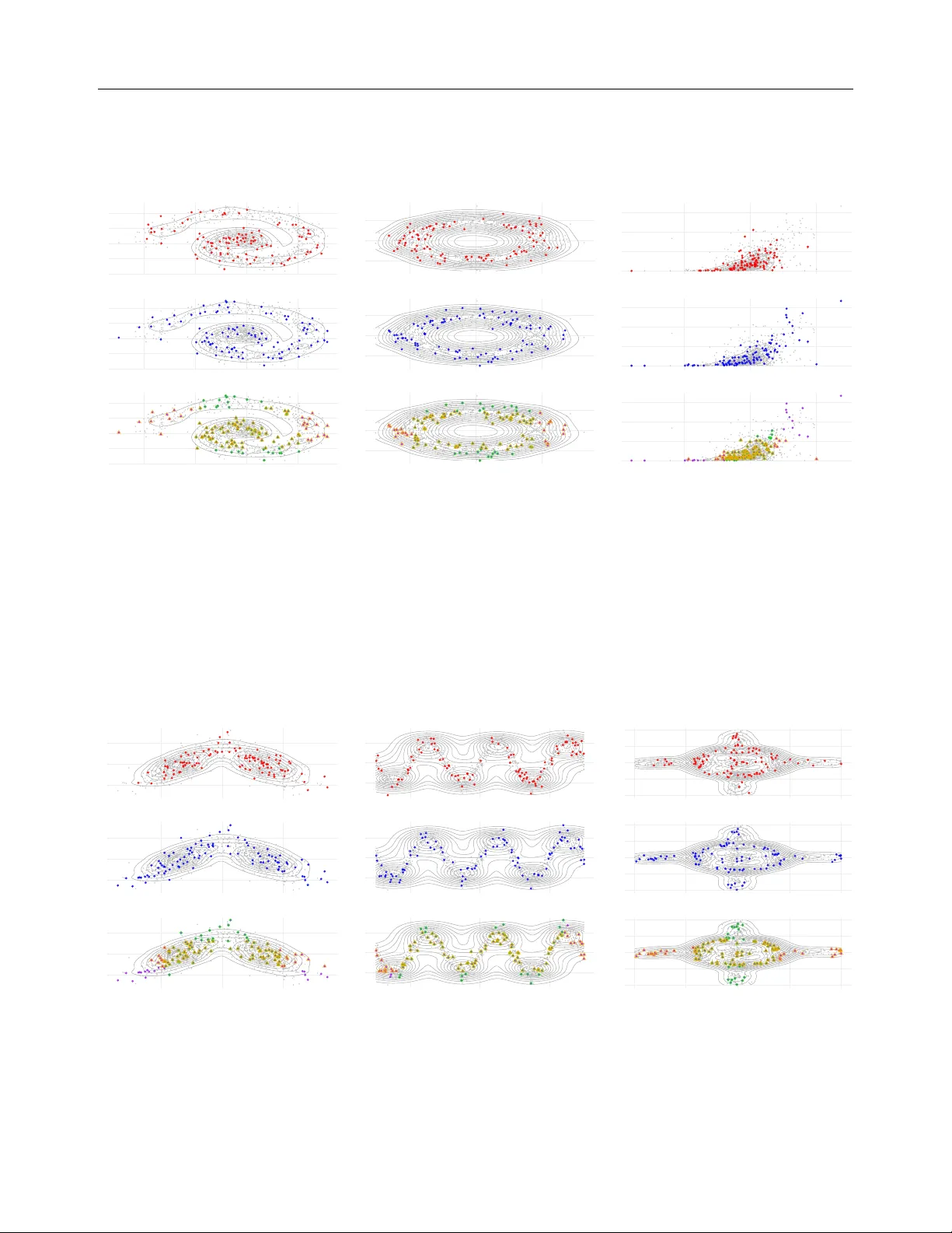
Scalable Learning of Multiv ariate Distributions via Coresets Zeyu Ding Katja Ic kstadt Nadja Klein Alexander Mun tean u Simon Omlor Lamarr Institute for ML & AI, TU Dortm und Scien tiﬁc Computing Center, Karlsruhe Institute of T echnology Departmen t of Statistics, TU Dortm und Abstract Eﬃcien t and scalable non-parametric or semi-parametric regression analysis and den- sit y estimation are of crucial imp ortance to the ﬁelds of statistics and mac hine learn- ing. Ho wev er, a v ailable methods are lim- ited in their abilit y to handle large-scale data. W e address this issue by dev eloping a nov el coreset construction for m ultiv ariate condi- tional transformation models (MCTMs) to enhance their scalability and training eﬃ- ciency . T o the best of our kno wledge, these are the ﬁrst coresets for semi-parametric dis- tributional models. Our approach yields sub- stan tial data reduction via importance sam- pling. It ensures with high probability that the log-likelihoo d remains within m ultiplica- tiv e error bounds of (1 ± ε ) and thereby main tains statistical model accuracy . Com- pared to con ven tional full-parametric models, where coresets ha ve b een incorp orated b e- fore, our semi-parametric approach exhibits enhanced adaptability , particularly in sce- narios where complex distributions and non- linear relationships are present, but not fully understo od. T o address numerical prob- lems associated with normalizing logarith- mic terms, w e follow a geometric appro xi- mation based on the conv ex h ull of input data. This ensures feasible, stable, and ac- curate inference in scenarios in volving large amoun ts of data. Numerical exp erimen ts demonstrate substan tially impro ved compu- tational eﬃciency when handling large and complex datasets, thus laying the foundation for a broad range of applications within the statistics and machine learning communities. 1 INTR ODUCTION In to da y’s era of Big Data, the v ast volume and in- creasing complexity of data in many real-world ap- plications p ose new c hallenges to statistics and ma- c hine learning. T raditional metho ds require intense computing times on large data and straigh tforward solutions such as uniform subsampling may lead to infeasible solutions. They often rely on strong mod- eling assumptions that are to o restrictive to capture complicated phenomena accurately . These limitations demand computationally eﬃcient and scalable tech- niques for more ﬂexible m ultiv ariate mo dels. T o address the need of scalable learning, the method of c or esets receiv ed a lot of atten tion in recent years. It aims to sample or select a relatively small but repre- sen tative subset of the original data that can b e used to accurately approximate the ob jective function for an y solution, thereb y signiﬁcantly reducing comput- ing, memory and storage requirements (Phillips, 2017; Mun teanu and Sch wiegelshohn, 2018). Ho wev er, most of the existing coreset literature fo- cused on clustering, linear regression, or generalized linear models that can handle only relativ ely sim- ple and limited distributional assumptions. Little researc h has b een conducted on more ﬂexible non- parametric, semi-parametric or highly non-linear mul- tiv ariate mo dels. This gap b ecomes more critical as the mac hine learning and statistics comm unities in- creasingly rely on complex distributional regression and estimation metho dologies including not only mul- tiv ariate features but also multiv ariate outcomes. 1.1 Brief In tro duction to MCTMs In this pap er, we speciﬁcally focus on multiv ariate con- ditional transformation mo dels (MCTMs; Klein et al., 2022), whic h hav e the unique adv an tage of mo deling b oth unconditional and conditional distributions, non- linear dependence structures, and ﬂexible eﬀects of fea- tures. The fundamental idea of MCTMs is to model marginal distributions non-parametrically via mono- Scalable Learning of Multiv ariate Distributions via Coresets tonic transformation functions. Multiple univ ariate distributions are then com bined into a multiv ariate distribution via a c opula , that contributes all infor- mation required to model the m ultiv ariate dependence structure. Sklar’s Theorem (Sklar, 1959) is well-kno wn and states that every multiv ariate distribution can b e comp osed and represented in that wa y . Of course, represen ting and calculating suc h a mo del explicitly in a lossless w ay for arbitrary multiv ariate distribu- tions may require solving inﬁnite-dimensional numeri- cal problems whic h is arguably not practical. MCTMs thus formulate a semi-parametric mo del that rely on the monotonic univ ariate transformations b e- ing approximated as a linear com bination of Bernstein p olynomial basis functions whose choice ensures mono- tonicit y of the composed functions. The dependence structure b etw een the univ ariate output components is imp osed by a Gaussian copula (Song, 2000). W e note that those mo deling choices ma y b e replaced by diﬀer- en t functional basis families and diﬀeren t copulas, but w e stress and demonstrate that it is not as restrictive as it may seem. Notice that, although Gaussian copu- las are centrally symmetric, the resulting model need not b e symmetric unless all marginal distributions are symmetric as w ell, see for instance the density con tour plots in Figures 2 to 6 in Section E.1.2. F or the sake of a concise presen tation, we restrict our- selv es to unconditional densit y estimation without fea- tures. See (Klein et al., 2022) for details and an ex- tension to the conditional case of distributional regres- sion. The goal is to learn the density f Y ( y ) of a J - dimensional random v ector Y = ( Y 1 , . . . , Y J ) T ∈ R J and its distribution function F Y ( y ) = P ( Y ≤ y ) = P ( h ( Y ) ≤ h ( y )). This in v olves a bijective, strictly monotonically increasing transformation function h : R J → R J estimated from the data. It maps Y to another random v ector Z ∈ R J that follo ws some con venien t reference distribution. In particular, the common marginal distribution P Z of the comp onents Z j ∼ P Z , j ∈ [ J ] is a mo deling c hoice and is assumed to not dep end on the data. It thus holds that h ( Y ) = ( h 1 ( Y ) , . . . , h J ( Y )) T d = ( Z 1 , . . . , Z J ) T = Z . F urthermore, it is assumed that each comp onent h j can b e expressed as a linear combination of strictly monotonically increasing marginal transforma- tion functions ˜ h j : R → R of the form h j ( y 1 , . . . , y j ) = λ j 1 ˜ h 1 ( y 1 ) + . . . + λ j j ˜ h j ( y j ) , where λ j l , l ≤ j are the unrestricted entries of a J × J lo wer triangular matrix Λ, suc h that Σ = Λ − 1 (Λ − 1 ) T is the co v ariance matrix of Z . Hence, Λ describ es the conditional dependencies b etw een the J compo- nen ts. The functions ˜ h j ( y j ) , j ∈ [ J ], are scaled marginal transformations, eac h of which carry an in- tercept term and together allo w the generation of ar- bitrary marginal distributions. The marginal trans- formations are mo deled semi-parametrically via some basis functions a j : R → R d and basis co eﬃcients ϑ j ∈ R d . The a j are c hosen, for example, to b e Bernstein p olynomials which allo w for a con v enient w ay to imp ose monotonicity . The unknown mo del pa- rameters are collected in the v ector θ = ( ϑ T , λ T ) T . F or consistency with other coreset literature, w e con- sider minimizing the negativ e log-lik eliho o d, or sp ecif- ically the sum of loss contributions of each data p oint y i ∈ R J , i ∈ [ n ] , to the negative log-lik eliho o d, whic h is equiv alen t to calculating the maximum likelihoo d estimator ˆ θ n = argmin θ =( ϑ T ,λ T ) T f ( θ ), where f ( θ ) = n X i =1 1 2 J X j =1 j − 1 X ȷ =1 λ j ȷ a ȷ ( y iȷ ) T ϑ ȷ + a j ( y ij ) T ϑ j ! 2 − log ( a ′ j ( y ij ) T ϑ j ) . (1) See (Klein et al., 2022) for details and a deriv ation of the log-likelihoo d and its gradients. MCTMs can b e ﬁtted to data by optimizing the linear basis co eﬃ- cien ts ϑ of univ ariate transformation models and the co v ariance structure of the Gaussian copula, which is parametrized through the unrestricted entries of the lo wer triangular matrix of the mo diﬁed Cholesky fac- tor Λ. MCTMs can thus b e seen as a multiv ariate ex- tension of univ ariate conditional transformation mo d- els (CTMs; Hothorn et al., 2014) to handle multi- dimensional outputs and their dep endence structure. As can b e seen in Equation (1), the log-likelihoo d function of an MCTM con tains b oth quadratic and logarithmic parts in terms of the parameters to op- timize. The quadratic part is numerically tractable and can be reformulated in a w a y that enables han- dling within the framework of ℓ 2 -subspace em beddings (W o o druﬀ, 2014), in particular via ℓ 2 lev erage score subsampling (Drineas et al., 2006; Rudelson and V er- sh ynin, 2007). The logarithmic part is kno wn to b e unstable and computationally burdensome when opti- mizing mo dels to ﬁt large-scale datasets. Considering sensitivit y sampling for similarly structured loss func- tions has required sp ecial eﬀorts and nov el techniques in recen t w ork on Poisson regression models (Lie and Mun teanu, 2024). F or the MCTMs considered here, the situation is even more aggra v ated since the terms that show up in the log-lik eliho o d do not directly de- p end on the plain data, but instead on the p olyno- mial basis transformations in the quadratic part and on their deriv atives in the logarithmic part. Zeyu Ding, Katja Ic kstadt, Nadja Klein, Alexander Mun teanu, Simon Omlor 1.2 Our Goals and Con tributions W e develop the ﬁrst coreset approximation framew ork for MCTMs, aiming to ac hieve the following goals. 1. Signiﬁcan t computational reduction whil e guaran teeing an accurate log-lik eliho o d appro x- imation. By combining ℓ 2 lev erage score sampling with a geometric con vex-h ull approximation, we pro- vide a (1 ± ε )-factor log-lik eliho o d approximation for MCTMs using only a small fraction of the data. 2. Solving the problem of unstable v alues of log- arithmic terms. W e construct corese ts separately for a ( y ) that represent p olynomial basis transforma- tions of plain data y , and their respective deriv atives a ′ ( y ). This allo ws to use standard metho ds for the for- mer part. F or the second part, extending recen t prior w ork of Lie and Muntean u (2024), our metho d includes p oin ts to av oid extreme directions where the logarithm tends to inﬁnit y or pro duces infeasible solutions. 3. Compatibilit y with other p opular probabilis- tic mo dels: MCTMs build a ﬂexible semi-parametric framew ork that has connections to contemporary ma- c hine learning metho ds such as deep learning and nor- malizing ﬂows (Kobyzev et al., 2021; Papamak arios et al., 2021). By scaling up MCTMs, our coresets bring signiﬁcant sp eedup and scaling p ossibilities to do wnstream learning tasks that build up on MCTMs. Theoretically , we develop a lev erage score and sen- sitivit y sampling analysis along with a conv ex h ull appro ximation scheme to provide a small subset of data. W e pro ve that it appro ximates the log-likelihoo d within a m ultiplicative (1 ± ε ) factor to the full dataset. Empirically , we demonstrate through simulated and real-w orld data exp eriments that the metho d oﬀers sig- niﬁcan t beneﬁts for large-scale data: increased compu- tational eﬃciency and scalabilit y , preserving the orig- inal mo del ﬁt, likelihoo d ratio, and estimation bias. W e summarize our main contributions as follows: 1. The ﬁrst coresets for the MCTM frame- w ork. T o the best of our knowledge, we are the ﬁrst to develop a coreset construction metho d for MCTMs, ﬁlling the gap of data reduction tech- niques for highly ﬂexible semi-parametric mo del ﬁtting metho ds for multiv ariate distributions. 2. Conv ex h ull based stabilization of logarith- mic normalizing terms. Numerical issues of logarithmic terms in the log-lik eliho o d are elim- inated based on prior work (Lie and Mun teanu, 2024) b y a conv ex-hull approximation of the deriv ative a ′ ( y ) of transformed data y . The prop- erties of this geo metric approximation are in v es- tigated theoretically and empirically . 3. Illustrative large-scale data scenarios. W e il- lustrate through exp eriments with simulated and real-w orld data that our new metho d op erates more eﬃciently than using the original large-scale data. A t the same time it retains almost the same mo del ﬁt as the original full-data estimation, il- lustrating our theoretical guaran tees in practice. 1.3 Related W ork Probabilistic T ransformation Mo dels. Origi- nally restricted to univ ariate outputs, Hothorn et al. (2014) prop osed a b o osting approach for estimating a monotonically inv ertible function that transforms the output v ariable to a conv enient, data indep en- den t distribution (e.g., standard normal). This trans- formation function is a semi-parametric, monotonic spline approximation that can dep end on input v ari- ables in a ﬂexible manner. This framework indirectly mo dels the full conditional distribution of the output and was later extended tow ards an entirely lik eliho o d- based approac h, known as most likely tr ansformations (Hothorn et al., 2018). Klein et al. (2022) built on this approac h using likelihoo d inference. They dev elop ed MCTMs that can estimate the joint conditional distri- bution of a m ultiv ariate resp onse directly based on the features. The original work of Klein et al. (2022) con- siders datasets of up to ten thousand observ ations and up to ten-dimensional outputs. In con trast to previ- ous probabilistic methods, MCTMs directly estimate the join t distribution function of a m ultiv ariate output v ector, av oiding the loss of information that would re- sult from mo deling only the mean or quantiles. T ransformation models are closely related to normal- izing ﬂo ws (NFs; Kob yzev et al., 2021; Papamak ar- ios et al., 2021), which are p opular in mac hine learn- ing. W e elab orate on this connection in Section D. The main idea of b oth approaches is to apply a data- driv en transformation suc h that the transformed v ari- able follows a standard normal or some other conv e- nien t distribution. How ev er, NFs transform their in- put via some kind of deep neural netw ork as a black b o x, whereas our model implemen ts a semi-parametric transformation using a Bernstein p olynomial basis, whic h remains analytically tractable. NFs are most commonly employ ed as ﬂexible v ariational distribu- tions in machine learning, whereas our fo cus is on mo deling the distribution of multiv ariate data along with their dep endence structure. MCTMs hav e also b een extended tow ards regression, where density es- timation is conditioned on feature v ariables. The lin- ear underlying structure of transformation functions of MCTMs hav e the great adv antage of enhancing inter- pretabilit y compared to the neural netw ork approach Scalable Learning of Multiv ariate Distributions via Coresets of NFs. F or instance, in MCTMs w e can directly in ter- pret the dep endencies betw een marginal comp onents of the outcome and clearly separate these eﬀects from those mo deling the marginal distributions. F urther, MCTMs are lik eliho o d-based and therefore yield ac- cess to conﬁdence in terv als via b o otstrapping. Coresets for Large-Scale Statistical Mo deling. The main idea of the coreset metho d is to select the most imp ortant subset of data based on their contri- bution to the ob jective function (e.g., log-likelihoo d or loss) and reweigh t them, so that training the mo del on this subset closely appro ximates the results of the original dataset. Early works on coresets fo cus on parametric mo dels, suc h as linear regression (Clark- son, 2005; Drineas et al., 2006; Dasgupta et al., 2009) or generalized linear mo dels (Muntean u et al., 2018; Molina et al., 2018; Muntean u et al., 2022; Lie and Mun teanu, 2024; F ric k et al., 2024). These also make up the bulk of work on coresets for statistical mo dels. Inferring whole probabilit y distributions received rela- tiv ely little atten tion in the coreset literature. Among them are coresets for univ ariate kernel density esti- mation (Phillips and T ai, 2018, 2020; Charik ar et al., 2020). Ba y esian coreset based mo dels focus on multi- v ariate parameter distributions rather than multiv ari- ate outcomes (Gepp ert et al., 2017; Huggins et al., 2016; Campbell and Broderick, 2018; Ding et al., 2024). T o our kno wledge, the only attempt to learn m ultiv ariate data distributions using coresets for scal- abilit y has b een made in the con text of dep endency net works that infer inter-v ariable dep endencies with graph structure (Molina et al., 2018). This approach is again comp osed of multiple parametric mo dels. In summary , the coreset metho d has sho wn great po- ten tial in improving the eﬃciency of regression models and Bay esian inference. Ho wev er, we stress that these metho ds hav e to date b een mainly developed for para- metric mo dels, e.g., (generalized) linear mo dels. V ery limited w ork has considered more complex and ﬂexible non- or semi-parametric distribution models for multi- v ariate outputs. Our attempt to combine coresets with MCTMs is, to the b est of our kno wledge, the ﬁrst of its kind, lev eraging the ﬂexibility of multiv ariate distri- butional regression with eﬃcient data reduction. Our w ork ﬁlls the gap in the metho dology for inference of large-scale m ultiv ariate distributional mo dels. 2 MCTM CORESET CONSTR UCTION Considering the MCTM mo del whose negative log- lik eliho o d function can b e deﬁned as in Equation (1), the goal of the coreset approach is to obtain a small subset C ⊂ D of data, such that the appro ximation of the original likelihoo d function is b ounded within a factor (1 ± ε ). The full details and pro ofs of our construction are deferred to Section A. After applying the basis functions a and their deriv a- tiv es a ′ to the raw data, w e can assume that for ( i, j ) ∈ [ n ] × [ J ] we are given data points a ij : = a j ( y ij ) ∈ R d and similarly for the deriv ativ es we hav e a ′ ij : = a ′ j ( y ij ) ∈ R d . W e use A, A ′ ∈ R nJ × d to denote the corresp onding data matrices. Additionally , we as- sume that there is an in tercept, i.e., that for each ( i, j ) the ﬁrst co ordinate of b oth a ij and a ′ ij is 1 to make it consisten t with the presence of intercepts in the trans- formation functions h deﬁned b efore, in Section 1.1. No w for i ∈ [ n ] , j ∈ [ J ] consider the function f ( a ij , ϑ, λ ) = 1 2 ( P j k =1 λ j,k ϑ k a ij ) 2 − log ( ϑ j a ′ ij ) whic h is the negative logarithm of the corresp onding likelihoo d comp onen t g ( i, j ) = ϑ j a ′ ij exp( − 1 2 ( P j k =1 λ j,k ϑ k a ij ) 2 ). W e assume that for all i ∈ [ n ] , j ∈ [ J ] and all c hoices of parameters it holds that g ( i, j ) ≤ c for some constan t c ∈ R ≥ 1 . This is a natural Lipschitz-t yp e restriction ensuring that the distribution function has a smo oth transition from 0 to 1 preven ting sudden jumps. Note that this is equiv alent to − ln( g ( i, j )) ≥ − ln( c ). W e further add to the nJ loss contributions a total shift of log N = nJ (ln( c ) + 1). This corresponds to a normalization term N that ensures non-negativity and th us allo ws a relativ e appro ximation to be meaningful. Crucially , it do es not aﬀect the optimization because it is indep endent of the parameters that we optimize. In the following, w e sample with probabilities that are larger than the ℓ 2 lev erage scores plus a uniform term and add the conv ex h ull of { a ′ ij | i ∈ [ n ] , j ∈ [ J ] } . This yields a coreset for the loss function f ( A, ϑ, λ ) to b e minimized in Equation (1). Let w ∈ R n × J b e a weigh t v ector. W e split the weigh ted version of f in to three parts (weigh ts w ij are omitted in the unw eighted case): 1) squared part: f 1 ( A, ϑ, λ, w ) = 1 2 X ( i,j ) ∈ [ n ] × [ J ] w ij j X k =1 λ j,k ⟨ ϑ k , a ij ⟩ ! 2 2) p ositiv e log part: f 2 ( A, ϑ, λ, w ) = X ( i,j ) ∈ [ n ] × [ J ] w ij max { log( ⟨ ϑ j , a ′ ij ⟩ ) , 0 } 3) negativ e log part: f 3 ( A, ϑ, λ, w ) = X ( i,j ) ∈ [ n ] × [ J ] w ij max {− log( ⟨ ϑ j , a ′ ij ⟩ ) , 0 } 1) Squared Part. W e let u i = sup ∥ x ∥ 2 =1 | M i x | 2 ∥ M x ∥ 2 2 for the i -th row of a matrix M denote their ℓ 2 lev erage score. W e show that sampling prop ortionally to the ℓ 2 lev erage score s preserves the squared part f 1 . Giv en Zeyu Ding, Katja Ic kstadt, Nadja Klein, Alexander Mun teanu, Simon Omlor ro ws a ij ∈ R d where i ∈ [ n ] and j ∈ [ J ], we are lo oking for an ε -coreset, whic h is giv en b y a matrix comprising a subset of rows indexed b y S ⊆ [ n ] × [ J ] and corre- sp onding w eigh ts w i,j for ev ery ( i, j ) ∈ S , such that for all ϑ 1 , . . . , ϑ J ∈ R d and λ ∈ R J × J it holds that       n X i =1 J X j =1 j X k =1 λ j,k ⟨ ϑ k , a ij ⟩ ! 2 − X ( i,j ) ∈ S w i,j j X k =1 λ j,k ⟨ ϑ k , a ij ⟩ ! 2       ≤ ε   n X i =1 J X j =1 j X k =1 λ j,k ⟨ ϑ k , a ij ⟩ ! 2   . T o this end, we arrange data points in a matrix suc h that sampling rows of this matrix yields a coreset for the function deﬁned abov e. W e set B ∈ R nJ × dJ 2 to b e the matrix whose ro ws equal ( b iJ + j ) k = a il if k = ( j − 1) J + l for some l ∈ [ J ] and ( b iJ + j ) k = 0 otherwise. Then B consists of n v ertically stack ed blocks B i , for i ∈ [ n ]. The i -th blo ck is deﬁned by B i =        b i 0 0 0 · · · 0 0 b i 0 0 · · · 0 0 0 b i 0 · · · 0 . . . . . . . . . . . . · · · 0 0 0 0 0 · · · b i        ∈ R J × dJ 2 , where b i = ( b i 1 , b i 2 , . . . , b iJ ). The idea is that for an y p ossible parametrization, the squared part can b e rep- resen ted by a pro duct of the new matrix B with the v ector θ = ( ϑ T , λ T ) T . An ε -subspace em bedding for ℓ 2 is therefore suﬃcien t to appro ximate the squared part, i.e., it yields that ∀ θ : ∥ B ′ θ ∥ 2 2 = (1 ± ε ) ∥ B θ ∥ 2 2 , where B ′ consists of few w eigh ted ro ws subsampled from B according to their ℓ 2 lev erage scores (W o o druﬀ, 2014). Lemma 2.1. Ther e exists a c or eset S for f 1 of size O ( J 2 d/ε 2 ) which c an b e c ompute d in time O (nnz( B ) log( nJ ) + poly( dJ )) and with high pr ob a- bility by sampling and r eweighting ac c or ding to the ℓ 2 lever age sc or es of B , wher e nnz( B ) denotes the numb er of non-zer o entries of B . We then have | f 1 ( A, ϑ, λ ) − f 1 ( A ( S ) , ϑ, λ, w ) | ≤ εf 1 ( A, ϑ, λ ) , wher e A ( S ) denotes the r estriction of A to the indic es in S . 2) P ositiv e Logarithmic Part. W e now turn our atten tion to the positive logarithmic part f 2 . This is going to b e handled using the sensitivit y framew ork, whic h generalizes the previous leverage score sampling for the ℓ 2 norm to more general families of functions. W e refer to Section B for details. First of all, w e bound the VC dimension of the logarithmic function. This is done in a standard wa y . Using strict monotonicity , the logarithmic function of the inner pro duct can b e in verted (resp ecting their domain and range), relating it to linear classiﬁers in d dimensions. The latter hav e a VC dimension of d + 1, which is kno wn from classic learning theory (Kearns and V azirani, 1994). The second part is b ounding the total sensitivity , whic h is the sum of all sensitivity scores s i = sup ϑ,λ f 2 ( a ij ,θ,λ ) P f 2 ( a ij ,θ,λ ) of single data point con tribu- tions. T o bound this v alue, we lev erage that for all parameters λ and ϑ it holds that ln( ϑ j a ′ ij ) − 1 2 ( w i,j P j k =1 λ j,k ϑ k a ij ) 2 ≤ ln( c ) , which allows us to relate the con tribution of the logarithmic part to the squared part up to a constant γ > 1 such that s i ≤ γ ( u i + 1 /n ). This allows to reuse the ℓ 2 lev erage scores for this part as w ell, alb eit with an additional uniform comp onen t, and with an increase of the sample size, whic h comes from incorporating the VC dimension and the Lipsc hitz bound c . W e also note that the ε -error is relativ e to f 1 instead of f 2 directly . Lemma 2.2. Assume that S is a sample c onsisting of O ( J 2 d 2 ln( cdJ ) c 6 /ε 2 ) p oints dr awn with pr ob ability p i ≥ α ( u i + 1 /n ) , wher e α ∈ O ( J 2 d ln( cdJ ) c 6 /ε 2 ) . Then with high pr ob ability it holds that | f 2 ( A, ϑ, λ ) − f 2 ( A ( S ) , ϑ, λ, w ) | ≤ εf 1 ( A, ϑ, λ ) , wher e A ( S ) denotes the r estriction of A to the indic es in S . 3) Negativ e Logarithmic Part. Next, w e handle the remaining negativ e logarithmic part given by f 3 . W e note that it has an asymptote at 0 , precluding ﬁnite b ounds on the sensitivity . W e handle this similarly to (Lie and Mun teanu, 2024) by restricting the optimiza- tion space to D ( η ) = { ( ϑ, λ ) | ∀ ( i, j ) ∈ [ n ] × [ J ] : ⟨ ϑ j , a ′ ij ⟩ > η } comprising only solutions for whic h the inner pro duct is b ounded aw a y b y η ≥ 0 from zero. Setting η = 0 corresp onds to the original domain. 1 By av oiding high sensitivity p oints in this w ay , f 3 can b e bounded in terms of uniform sensitivities together with the V C dimension b ound d + 1 and appro ximated b y inv oking the sensitivity framework again. Lemma 2.3. L et ( ϑ ∗ , λ ∗ ) b e an optimal solution. Then ther e exist ( ϑ, λ ) ∈ D ( η ) with | f ( A, ϑ, λ ) − f ( A, ϑ ∗ , λ ∗ ) | ≤ 2 J η f 1 ( A, ϑ ∗ , λ ∗ ) + J η n + J 2 η 2 n . F ur- ther, if S is a sample c onsisting of α p oints dr awn with pr ob ability p i ≥ α/n wher e α ∈ O ( d ln( cdJ ) /η 2 ) c ombine d with al l p oints that ar e on the c onvex hul l of { a ′ ij | i ∈ [ n ] , j ∈ [ J ] } . Then with high pr ob abil- ity, it holds for al l ( ϑ, λ ) ∈ D ( η ) that | f 3 ( A, ϑ, λ ) − f 3 ( A ( S ) , ϑ, λ, w ) | ≤ η f 1 ( A, ϑ, λ ) + η n , wher e A ( S ) de- notes the r estriction of A to the indic es in S . Main Result. W e get the follo wing theorem by a union bound ov er Lemmas 2.1 to 2.3 and adding 1 The ﬁnal choice will b e η = Θ( ε ) and negativ e v alue correction to the p ositive domain was common practice in (Klein et al., 2022) b efore our theoretical inv estigations. Scalable Learning of Multiv ariate Distributions via Coresets up their error b ounds using the triangle inequality . The additive errors of Lemma 2.3 are further charged against the optimal cost using the normalization given b y log N , see ab o ve at the b eginning of Section 2. Theorem 2.4. Assume that S is a sample c onsisting of O ( J 2 d 2 ln 3 ( cdJ ) c 6 /ε 2 ) p oints dr awn with pr ob ability p i ≥ α ( u i + 1 /n ) , wher e α ∈ O ( J 2 d ln 3 ( cdJ ) c 6 /ε 2 ) c ombine d with al l extr eme p oints ( i, j ) ∈ [ n ] × [ J ] that ar e on the c onvex hul l of { a ′ ij | i ∈ [ n ] , j ∈ [ J ] } . Then with high pr ob ability it holds for any ( ϑ, λ ) ∈ D ( η ) that | f ( A, ϑ, λ ) − f ( A ( S ) , ϑ, λ, w ) | ≤ εf ( A, ϑ, λ ) and ther e exists ( ϑ, λ ) ∈ D ( η ) such that f ( A, ϑ, λ ) ≤ (1 + O ( ε )) f ( A, ϑ ∗ , λ ∗ ) , for an optimal solution ( ϑ ∗ , λ ∗ ) . The formal proof can b e found in Section A. W e remark that the conv ex h ull can comprise Ω( nJ ) p oin ts, ho w ever, diﬀerent η -kernel coresets of size Θ(1 /η ( d − 1) / 2 ) exist for the problem (Agarw al et al., 2004; Chan, 2004), survey ed in (Agarwal et al., 2005), in the ﬁeld of computational geometry . These η - k ernels also match the requiremen ts of the shifted do- main D ( η ). W e discuss one particular choice (Blum et al., 2019) in the exp erimental section 3 b elow. Lo w er Bounds. W e also give t wo low er b ounds un- der diﬀerent natural assumptions on the λ co eﬃcients that deﬁne the dep endence structure of the Gaussian copula. These indicate the limitations of coresets for MCTMs and show that our upper bounds leav e only small gaps. The details are again in Section A. Lemma 2.5. Ther e exists a dataset { a ij } i ∈ [ n ] j ∈ [ J ] such that any c or eset for MCTMs with ε < 1 has size at le ast Ω( dJ 2 ) even if λ ij = 0 for al l i, j ∈ [ n ] with j > i and | λ ij | ≤ 1 for al l i, j ∈ [ J ] . Lemma 2.6. Ther e exists a dataset { a ij } i ∈ [ n ] j ∈ [ J ] such that any c or eset for MCTMs with ε < 1 has size Ω( dJ ) even if λ ii = 1 for i ∈ [ J ] and λ ij = 0 for i < j . 3 EMPIRICAL EV ALUA TION In this section, w e systematically inv estigate coreset data reduction tech niques for MCTMs with large-scale data for a v ariety of 2-dimensional data generation pro cesses as well as t w o m ulti-dimensional, large-scale, real-w orld applications. Our ob jectiv es are to (i) validate the eﬀe ctiveness of the pr op ose d sampling and c onvex hul l algorithm for MCTMs at ﬁtting diﬀer- ent distributions, diﬀer ent c orr elation structur es, and non-line ar or he avy-taile d sc enarios, and to (ii) quantify and c omp ar e the p erformanc e of uniform sampling, pur e ℓ 2 lever age sc or e sampling, and our sensitivity sampling c ombine d with the c onvex hul l ap- pr oximation on various metrics. Our algorithms are stated in Section C. In particu- lar, our sensitivity sampling is detailed in Algorithm 1. As con v ex h ull approximation, w e implemented (Blum et al., 2019) given in Algorithm 2. F or mild data, i.e., data that admits an η -kernel b elow the Ω(1 /η ( d − 1) / 2 ) lo wer b ound, it yields an η -kernel of size O ( k ∗ /η 2 ), where k ∗ is the smallest p ossible size. 2 All exp eriments w ere carried out on a 2021 MacBo ok Pro equipped with an Apple M1 Pro chip and 16 GB of RAM. The co de to repro duce our exp eriments is a v ailable at https://github.com/zeyudsai/mctmcoreset/ . 3.1 Sim ulation Study on 2-Dimensional Data W e conduct a set of 2-dimensional data sim ulation exp erimen ts encompassing diﬀerent dependence struc- tures to v alidate the adv antages of our prop osed core- set approach ( ℓ 2 -h ull) ov er simple lev erage scores ( ℓ 2 - only) and uniform sampling as baselines. All exp erimental results can b e found in Section E. In particular, complete descriptions of 14 data generation pro cesses (DGPs) are sp eciﬁed in Section E.1.1. Ad- ditional density contour plots that visualize the DGPs are in Section E.1.2. T able 1 summarizes the simulation results for ﬁv e rep- resen tative scenarios. The exp erimental results clearly sho w that even in the extreme case of ﬁtting the model using only a few dozen p oints, our prop osed coreset metho d achiev es a satisfactory approximation. T o en- sure the reliabilit y of our exp erimental results, w e p er- formed 10 indep endent rep etitions of each simulation, to obtain the means and standard deviations of results. Based on the full exp erimental results in T ables 3 and 4 in Section E, we conclude that out of all 14 DGPs, our prop osed coreset metho d ( ℓ 2 -h ull) signiﬁcantly outp er- forms uniform subsampling in 12 scenarios, and fails to sho w an adv antage only in tw o scenarios, but never falls behind. Similarly , it also outperforms the plain ℓ 2 lev erage scores ( ℓ 2 -only). This suggests that our core- set metho d has a robust p erformance across a wide range of data dep endence structures, and is partic- ularly suitable for dealing with non-linearities, het- eroscedasticit y , complex dep endence structures, and m ultimo dality . Our results thus highlight the stabilit y and univ ersality of our metho d. Shortcomings in the t wo remaining scenarios, namely for t-copula and skew-t , show limitations for heavy- tailed distributions, when the coreset size is ﬁxed. These hav e a dense conv ex hull and thus require the size of the con vex hull approximation to b e increased in order to comp ensate and reduce the error. 2 Our theoretical results show that η = Θ( ε ) suﬃces, and in the exp eriments we simply choose η = 2 ε . Zeyu Ding, Katja Ic kstadt, Nadja Klein, Alexander Mun teanu, Simon Omlor T able 1: Performance comparison of coreset methods (coreset size = 30). Results show mean ± std o ver 10 runs. Relative improv ement: avg % improv ement across metrics. Best v alues highlighted in b old . Metho d ℓ 2 err. λ err. LR Imp.(%) DGP 1 ℓ 2 -h ull 2 . 56 ± 0 . 7 0 . 44 ± 0 . 1 1 . 54 ± 0 . 2 12 . 8 ℓ 2 -only 2 . 54 ± 0 . 6 0 . 51 ± 0 . 1 1 . 65 ± 0 . 3 1 . 6 uniform 4 . 91 ± 4 . 7 0 . 29 ± 0 . 2 1 . 94 ± 1 . 1 baseline DGP 2 ℓ 2 -h ull 1 . 76 ± 0 . 8 0 . 09 ± 0 . 1 1 . 03 ± 0 . 0 49 . 8 ℓ 2 -only 2 . 18 ± 0 . 8 0 . 10 ± 0 . 1 1 . 05 ± 0 . 0 38 . 8 uniform 3 . 08 ± 0 . 9 0 . 11 ± 0 . 1 1 . 21 ± 0 . 4 baseline DGP 3 ℓ 2 -h ull 2 . 60 ± 1 . 0 0 . 14 ± 0 . 1 1 . 07 ± 0 . 0 49 . 6 ℓ 2 -only 2 . 76 ± 0 . 9 0 . 16 ± 0 . 1 1 . 08 ± 0 . 0 43 . 7 uniform 4 . 14 ± 1 . 8 0 . 2 ± 0 . 1 1 . 42 ± 0 . 3 baseline DGP 4 ℓ 2 -h ull 2 . 51 ± 2 . 6 0 . 06 ± 0 . 0 1 . 33 ± 0 . 5 41 . 4 ℓ 2 -only 4 . 09 ± 4 . 3 0 . 07 ± 0 . 0 1 . 58 ± 0 . 5 9 . 0 uniform 4 . 11 ± 2 . 4 0 . 14 ± 0 . 1 1 . 47 ± 0 . 5 baseline DGP 5 ℓ 2 -h ull 2 . 07 ± 0 . 6 0 . 08 ± 0 . 0 1 . 07 ± 0 . 1 64 . 8 ℓ 2 -only 2 . 65 ± 0 . 8 0 . 08 ± 0 . 0 1 . 09 ± 0 . 1 58 . 4 uniform 4 . 47 ± 3 . 3 0 . 16 ± 0 . 1 1 . 63 ± 1 . 1 baseline 3.2 Real-W orld Data Exp erimen ts W e ev aluate our method on tw o large-scale multiv ari- ate datasets from diﬀeren t real-world applications. • F orest Co v er Data (Co vert yp e). The UCI Co vert yp e dataset (Black ard, 1998) contains n = 581 012 samples and 54 v ariables describing terrain at- tributes. W e fo cus on 10 contin uous v ariables (e.g., el- ev ation, slope, hillshade, distances) and a subsample of size n = 300 000. W e rep ort comparisons of ℓ 2 -h ull v er- sus ℓ 2 -only , uniform sampling on parameter ϑ error, λ error, log-likelihoo d ratio in T able 2. Additional base- lines include ridge lev erage scores (ridge-lss) and ro ot lev erage scores (ro ot-l2). F urther results and running times are presen ted in Figure 13 and in Section E. • Equity Returns. W e consider tw o sto ck-return datasets: one comprising 10 ma jor stocks’ forty-y ear daily returns ( n ≈ 10 000), and another with 20 sto c ks. Performances at v arying coreset sizes k ∈ { 50 , 100 , 200 , 300 } are summarized in T ables 5 and 6 in Section E, and Figure 1 visualizes the log-lik eliho o d ratio, parameter ℓ 2 distance and λ distance. W e refer to Section E.2 for further details on real- w orld data exp erimen ts. Across b oth real-world ap- plications, our prop osed ℓ 2 -h ull strategy outperforms uniform subsampling, and other baselines, achieving tigh ter log-lik eliho o d appro ximations and smaller pa- rameter errors at comparable running times. These results conﬁrm that coresets enable scalable, accurate MCTM ﬁtting on large, m ultiv ariate datasets. Through exp erimen ts on the real-v alued features of the Co vert yp e dataset (as shown in T able 2), w e ﬁnd that the prop osed coreset metho d (esp ecially the h ybrid sampling strategy com bining ℓ 2 sensitivit y with con- v ex hull appro ximation) signiﬁcan tly outp erforms uni- form sampling and other baselines at diﬀerent coreset sizes k ∈ { 50 , 100 , 200 , 500 } . In particular, when the coreset size is small (e.g., k = 50), where the p erfor- mance of uniform sampling deteriorates, our metho d can eﬀectively preserv e the approximation accuracy of the model, demonstrating the abilit y to capture imp or- tan t k ey data p oin ts. In addition, our coreset metho d remains stable and main tains its adv antage o ver uni- form sampling as the subset size increases. This in- dicates that our prop osed metho d not only eﬀectively reduces the computational cost on real-world datasets from several hours to a few seconds, but also accurately appro ximates the b enchmark MCTM model ﬁtted to the complete data, thus achieving eﬃcient and accu- rate large-scale m ultiv ariate probabilistic mo deling. T able 2: Cov ertype data p erformance for diﬀerent coreset sizes. Results: mean ± std ov er 5 trials. F or ℓ 2 distances, low er is b etter. F or log-lik eliho o d Ratio, closer to 1 is b etter. Best v alues highligh ted in b old . Size Metho d P aram L2 Lambda L2 LR k = 50 l2-h ull 23 . 4 ± 9 . 8 18 . 2 ± 12 . 2 11 . 4 ± 6 . 2 l2-only 40 . 7 ± 24 . 2 37 . 0 ± 26 . 6 71 . 8 ± 8 . 7 ridge-lss 30 . 8 ± 21 . 5 25 . 6 ± 24 . 3 51 . 7 ± 45 . 7 ro ot-l2 64 . 6 ± 10 . 4 63 . 2 ± 10 . 7 122 . 0 ± 96 . 1 uniform 52 . 6 ± 10 . 6 50 . 6 ± 10 . 9 84 . 8 ± 90 . 5 k = 200 l2-h ull 14 . 0 ± 3 . 1 7 . 4 ± 5 . 4 1 . 42 ± 0 . 13 l2-only 15 . 7 ± 2 . 3 10 . 1 ± 4 . 0 1 . 55 ± 0 . 33 ridge-lss 16 . 3 ± 2 . 2 11 . 5 ± 3 . 5 3 . 28 ± 5 . 0 ro ot-l2 28 . 2 ± 12 . 9 24 . 2 ± 15 . 7 14 . 5 ± 7 . 7 uniform 37 . 2 ± 4 . 6 35 . 2 ± 4 . 8 45 . 1 ± 16 . 2 k = 500 l2-h ull 11 . 1 ± 2 . 1 6 . 5 ± 3 . 5 1 . 07 ± 0 . 02 l2-only 15 . 9 ± 1 . 2 11 . 7 ± 1 . 5 1 . 12 ± 0 . 01 ridge-lss 16 . 3 ± 1 . 2 12 . 2 ± 1 . 5 1 . 27 ± 0 . 19 ro ot-l2 17 . 4 ± 9 . 0 12 . 7 ± 11 . 1 1 . 27 ± 0 . 11 uniform 25 . 3 ± 10 . 5 21 . 6 ± 12 . 8 20 . 0 ± 14 . 0 Bench. n = 100 k 0 0 1 n = 300 k 0 0 1 Our comparisons of size vs. empirical relativ e errors consider diﬀeren t metho ds at ﬁxed coreset sizes. In- stead, one could ev aluate the reduction in mo del size that our metho d achiev es compared to its comp etitors at a ﬁxed error level. How ev er, it is impractical to ﬁx the exact error in adv ance due to v ariability of random sampling. The reduction can b e seen in Figure 1 (and in similar ﬁgures in Section E) b y dra wing a horizon- tal line at an y desired error lev el to compare the re- quired sample sizes. The plots th us demonstrate that to ac hiev e the same log-lik eliho o d ratio or parameter estimate accuracy , uniform sampling t ypically requires a lot larger sample size than our prop osed metho d. Scalable Learning of Multiv ariate Distributions via Coresets Zoom X−Y 1 2 3 4 5 6 7 8 9 10 0 100 200 300 Coreset Size (k) LogLik Ratio (Coreset / Full) l2_hull l2_only uniform Stock returns 10D (Unconditional) Log−Likelihood Ratio Comparison (a) 10-sto ck log-likelihoo d ratio Zoom X 30 50 100 100 200 300 Coreset Size (k) L2 Distance (Coreset vs Full) l2_hull l2_only uniform Stock returns 10D (Unconditional) Parameter L2 Distance Comparison (b) 10-sto ck parameter ϑ distance Zoom X 1 10 100 100 200 300 Coreset Size (k) L2 Distance (..) l2_hull l2_only uniform Stock returns 10D (Unconditional) Lambda L2 Distance Comparison (c) 10-sto ck parameter λ distance Zoom X−Y 1 2 3 4 5 6 7 8 9 10 0 100 200 300 Coreset Size (k) LogLik Ratio (Coreset / Full) l2_hull l2_only uniform Stock returns 20D (Unconditional) Log−Likelihood Ratio Comparison (d) 20-sto ck log-likelihoo d ratio Zoom X 50 70 100 100 200 300 Coreset Size (k) L2 Distance (Coreset vs Full) l2_hull l2_only uniform Stock returns 20D (Unconditional) Parameter L2 Distance Comparison (e) 20-sto ck parameter ϑ distance Zoom X 1 3 10 30 100 200 300 Coreset Size (k) L2 Distance (..) l2_hull l2_only uniform Stock returns 20D (Unconditional) Lambda L2 Distance Comparison (f ) 20-sto ck λ distance Figure 1: Coreset p erformance comparison on sto ck-return data. T op row: 10 sto cks; b ottom row: 20 sto cks. Shaded bands indicate ± 1 standard deviation, and solid lines show the av erages ov er multiple rep etitions. 4 DISCUSSION AND EXTENSIONS W e elab orate on limitations and possible extensions that go b eyond the scop e of our pap er. Choice of copula and basis functions. The Gaus- sian copula has been chosen as an example for intr o- ducing small coresets to copula mo dels by using their close connection to ℓ 2 lev erage scores. W e demonstrate in our 2-dimensional examples that this already allo ws v ery ﬂexible modeling despite a sp eciﬁc formulation. Our coreset metho d will work as well for other log- conca ve copulas (with conv ex level sets). The idea is that suc h distributions are similar to a Gaussian b e- cause w e can ﬁnd a so-called John ellipsoid E that is enclosed in a level set and its expansion √ dE encloses the same lev el set. Then, we can derive lev erage scores from the quadratic form that describ es the ellipsoid as in (T uk an et al., 2020), instead of the leverage scores obtained from the data. Copulas with non-conv ex level sets could b e handled similarly , dep ending on the level sets b eing in some sense close to their conv ex h ull. Our coreset construction is agnostic to the c hoice of basis functions. The basis function family is thus sim- ply exc hangeable. W e relied on Bernstein polynomi- als as in prior work b y Klein et al. (2022) for con v e- nience, as they allow to easily accoun t for the required monotonicit y constraint while b eing ﬂexible enough to model arbitr ary marginal distributions. W e w ould th us not exp ect any signiﬁcant diﬀerence or gains when mo deling with alternative choices. How ever, there may b e computational issues to obtain a v alid CDF. F or in- stance B-splines hav e b een suggested b y Carlan et al. (2024). Their approac h is Ba y esian allowing to in- corp orate monotonicit y via appropriate prior c hoices, whic h is not directly applicable to our framew ork, but probably in teresting tow ards a Bay esian extension. Extending our metho ds to c onditional transformation mo dels would b e straightforw ard for a linear condi- tional structure; it only increases the dimension de- p endence by the num b er of features conditioned on. F or non-linear structures, the situation is more com- plicated and one would hav e to consider diﬀerent av ail- able coreset techniques, e.g., for a sp eciﬁc generalized linear mo del such as logit, probit, or Poisson. Dimension dependence. There are sev eral imp or- tan t asp ects regarding the dimension dep endence. First of all, w e note that densit y estimation (with prov- able guarantees) has principle d limitations for high- dimensional data. F or instance, it is kno wn that the empirical densit y approac hes the original densit y with an error of O (1 /n 1 /d ) in terms of W asserstein distance (Nguy en and Ho, 2022), th us requiring a sample size of n = O (1 /ε d ) to bring the error term in the order of ε . Existing w ork is thus limited to very few dimensions. Zeyu Ding, Katja Ic kstadt, Nadja Klein, Alexander Mun teanu, Simon Omlor Our 2-dimensional simulated examples are mainly mean t to visually demonstrate the mo del’s ﬂexibil- it y b eyond Gaussian structures, despite the limitation to Gaussian copulas. Our real-world exp eriments are conducted on 10 v ariables (Cov ertype) and 10 resp. 20 v ariables (Equity returns), exceeding the usual range. W e also note that for 10 dimensions and 7 ba- sis functions, the dimension of the resulting optimiza- tion problem is signiﬁcan tly more than one hundred. As described in Section E.2, for suc h dimensions and n ≈ 580 000 our standard laptop crashes when ﬁtting the full data. With our coreset reduction, we did not exp erience an y such scalability limitations. The coreset size speciﬁed in our theorem is O ( J 2 d 2 p olylog( J d )), and we giv e a close low er b ound of Ω( J 2 d ) corrob orating that our metho ds reducing the double-sum of squares to standard metho ds do not lift to dimensions higher than necessary and do not imp ose restrictions to the sp ectrum as in prior work (Huang et al., 2020) on comparable loss (only w.r.t. the squared part). The additional factor d in our upp er b ound is an artifact of the sensitivity framework used as a blac k-b ox in our analysis; recent optimal analyses (Mun teanu and Omlor, 2024a) suggest that this factor can b e eliminated via tighter chaining analyses. The con v ex h ull component, ho wev er, has exp onen- tial Θ(1 /η ( d − 1) / 2 ) worst-case complexity . Unfortu- nately , for high-dimensional data, one must rely on their ’mildness’ and to heuristics, or preselect a sub- set of the dimensions using leverage scores or classic PCA (T esc hke et al., 2024; Pearson, 1901). In our ex- p erimen ts, hea vy-tailed data turned out to be ’hard’, for whic h the appro ximation deteriorates at ﬁxed core- set size, and it requires an exp onential increase of the con vex hull comp onent to comp ensate for this eﬀect. Data streams and distributed data. These com- putational settings can b e realized via black-box re- ductions using coresets. If data are merely inserted (at p ossibly diﬀeren t sites) they can b e aggregated using Merge & Reduce (cf. Gepp ert et al., 2020; Muntean u, 2023). T o handle deletions, dynamic up dates, and sparsit y , one usually requires oblivious sketc hes (e.g., Mun teanu et al., 2021, 2023; Mai et al., 2023). Lever- age score sampling, conv ex hulls and John ellipsoids can also b e approximated in data streams (W o o druﬀ and Y asuda, 2022; Muntean u and Omlor, 2024b). 5 SUMMAR Y AND CONCLUSION Our pap er fo cuses on the c or eset approach to enhance eﬃciency and scalability of ﬁtting MCTM mo dels to large datasets. Despite MCTM’s adv antages in ﬂexi- bly mo deling complex multiv ariate joint distributions, its computational burden increases signiﬁcan tly with increasing sample size, even with mo derate output di- mension. This hinders its direct application to real- w orld Big Data scenarios. T o this end, we dev eloped a no vel coreset construction algorithm, which integrates subsampling based on ℓ 2 lev erage scores with con v ex h ull selection. On the one hand, the ℓ 2 lev erage scores ensure that the samples fo cus on particularly informa- tiv e observ ations. On the other hand, the conv ex hull captures the extreme v alue patterns of the distribu- tion. In exp erimen ts, it has b een demonstrated that our ℓ 2 -hull algorithm reduces the data to a negligible prop ortion of their original size. Moreov er, the ﬁt- ting accuracy (log-likelihoo d ratio, parameter ϑ, λ dis- tances) are virtually unchanged in contrast to pure ℓ 2 lev erage score sampling and the simplest uniform sam- pling. Our work comprehensively ev aluates fourteen 2- dimensional simulation scenarios and tw o multiv ariate real-w orld datasets with large sample sizes. Our ﬁnd- ings demonstrate that ℓ 2 -hull outp erforms uniform sampling in 12 out of 14 simulated scenarios. F ur- thermore, it ac hieves signiﬁcantly sup erior statistical p erformance in the con text of multiv ariate real-w orld data. The running time of ℓ 2 -hull is comparable to that of uniform sampling, y et it is neither inferior nor merely comparable to pure ℓ 2 lev erage score sampling. The main con tribution of this paper is the ﬁrst in tro- duction of the coreset metho d to the complex semi- parametric MCTM framew ork. Unlik e previous core- sets, which were limited to parametric mo dels such as (generalized) linear regression, w e prop ose a new sam- pling sc heme that naturally com bines ℓ 2 lev erage score sampling with iterative conv ex hull selection. This allo ws us to give a rigorous theoretical pro of of the error bounds, whic h ensure that do wnstream statisti- cal p erformance measures are retained when applied to large-scale data. F urthermore, we discuss the in- trinsic connection b etw een MCTMs and normalizing ﬂo ws (NFs), which hav e become p opular in machine learning recen tly: b oth of them map complex distri- butions to simple reference distributions through in- v ertible transformations, thus achieving highly ﬂexi- ble distribution mo deling. This not only provides a new p ersp ective on the connection of semi-parametric transformation mo dels with deep generative mo dels (Herp et al., 2025), but also op ens new researc h di- rections for inserting coreset tec hniques into NF mo d- els or combining MCTMs with NFs more closely in the future. F uture research directions of our coreset approac h include extensions to semi-parametric addi- tiv e or mixed mo dels or to Ba y esian settings. Online streaming updating, and distributed calculation of our coreset construction can b e explored to adapt to time- and lo cation-v arying data scenarios. Finally , it is an in triguing question how far our metho ds can b e gen- eralized to build coresets for NFs directly . Scalable Learning of Multiv ariate Distributions via Coresets Ac kno wledgemen ts W e thank the anon ymous reviewers for their v aluable commen ts. W e thank Pia Schreiber for her prelim- inary w ork on conv ex hull approximations. Alexan- der Mun teanu and Simon Omlor w ere supp orted by the German Research F oundation (DF G) – grant MU 4662/2-1 (535889065) and by the TU Dortmund – Cen ter for Data Science and Sim ulation (DoDaS). Zeyu Ding, Katja Ickstadt, and Simon Omlor ackno wl- edge the supp ort of BMBF and MKW.NR W within the Lamarr-Institute for Mac hine Learning and Arti- ﬁcial In telligence. Nadja Klein ac knowledges support b y the German Researc h F oundation (DFG) through the Emm y No ether grant KL3037/1-1. References Agarw al, P . K., Har-Peled, S., and V aradara jan, K. R. (2004). Approximating extent measures of p oints. J. ACM , 51(4):606–635. Agarw al, P . K., Har-P eled, S., V aradara jan, K. R., et al. (2005). Geometric appro ximation via coresets. Combi- natorial and computational ge ometry , 52(1):1–30. Blac k ard, J. (1998). Cov ertype. UCI Mac hine Learning Rep ository . DOI: h ttps://doi.org/10.24432/C50K5N. Blum, A., Har-Peled, S., and Raichel, B. (2019). Sparse appro ximation via generating p oint sets. ACM T r ansac- tions on Algorithms (T ALG) , 15(3):1–16. Campb ell, T. and Bro derick, T. (2018). Bay esian core- set construction via greedy iterativ e geo desic ascent. In Pr o c e e dings of the 35th International Confer enc e on Ma- chine Le arning (ICML) , pages 698–706. Carlan, M., Kneib, T., and Klein, N. (2024). Bay esian con- ditional transformation mo dels. Journal of the A meric an Statistic al Asso ciation , 119(546):1360–1373. Chan, T. M. (2004). F aster core-set constructions and data stream algorithms in ﬁxed dimensions. In Pr o c e e dings of the twentieth annual symp osium on Computational ge- ometry , pages 152–159. Charik ar, M., Kapralov, M., Nouri, N., and Siminelakis, P . (2020). Kernel density estimation through density con- strained near neighbor searc h. In Irani, S., editor, 61st IEEE A nnual Symp osium on F oundations of Computer Scienc e, FOCS 2020, Durham, NC, USA, Novemb er 16- 19, 2020 , pages 172–183. IEEE. Clarkson, K. L. (2005). Subgradient and sampling al- gorithms for ℓ 1 regression. In Pr oc e e dings of the 16th Annual ACM-SIAM Symp osium on Discr ete Algorithms (SODA) , page 257–266. Dasgupta, A., Drineas, P ., Harb, B., Kumar, R., and Ma- honey , M. W. (2009). Sampling algorithms and core- sets for ℓ p regression. SIAM Journal on Computing , 38(5):2060–2078. Ding, Z., Omlor, S., Ickstadt, K., and Mun teanu, A. (2024). Scalable Ba y esian p-generalized probit and lo- gistic regression. A dvances in Data A nalysis and Clas- siﬁc ation , pages 1–35. Drineas, P ., Mahoney , M. W., and Muth ukrishnan, S. (2006). Sampling algorithms for l 2 regression and ap- plications. In Pr oc e e dings of the Sevente enth Annual ACM-SIAM Symp osium on Discr ete Algorithms, SODA 2006, Miami, Florida, USA, January 22-26, 2006 , pages 1127–1136. ACM Press. F eldman, D. and Langberg, M. (2011). A uniﬁed frame- w ork for approximating and clustering data. In Pr o- c e e dings of the F orty-Thir d Annual A CM Symp osium on The ory of Computing (STOC) , page 569–578. F eldman, D., Schmidt, M., and Sohler, C. (2020). T urning Big Data in to tiny data: Constant-size coresets for k - means, PCA, and pro jective clustering. SIAM Journal on Computing , 49(3):601–657. F rick, S., Krivosija, A., and Muntean u, A. (2024). Scalable learning of item resp onse theory mo dels. In International Confer enc e on A rtiﬁcial Intel ligenc e and Statistics (AIS- T A TS) , pages 1234–1242. Gepp ert, L. N., Ic kstadt, K., Mun tean u, A., Queden- feld, J., and Sohler, C. (2017). Random pro jections for Ba yesian regression. Statistics and Computing , 27(1):79– 101. Gepp ert, L. N., Ic kstadt, K., Mun teanu, A., and Sohler, C. (2020). Streaming statistical mo dels via Merge & Reduce. Int. J. Data Sci. Anal. , 10(4):331–347. Herp, M., Brachem, J., Altenbuc hinger, M., and Kneib, T. (2025). Graphical transformation mo dels. arXiv:2503.17845 . Hothorn, T., Kneib, T., and B ¨ uhlmann, P . (2014). Con- ditional transformation mo dels. Journal of the R oyal Statistic al So ciety Series B: Statistic al Metho dolo gy , 76(1):3–27. Hothorn, T., M¨ ost, L., and B¨ uhlmann, P . (2018). Most lik ely transformations. Sc andinavian Journal of Statis- tics , 45(1):110–134. Huang, L., Sudhir, K., and Vishnoi, N. K. (2020). Coresets for regressions with panel data. In A dvanc es in Neur al Information Pro c essing Systems 33 (NeurIPS) . Huggins, J., Campbell, T., and Broderick, T. (2016). Core- sets for scalable Ba yesian logistic regression. In A dvanc es in Neur al Information Pr o c essing Systems (NeurIPS) , v olume 29, pages 4080–4088. Kearns, M. J. and V azirani, U. V. (1994). A n Intr o duction to Computational L e arning The ory . MIT Press, Cam- bridge, MA, USA. Klein, N., Hothorn, T., Barban ti, L., and Kneib, T. (2022). Multiv ariate conditional transformation models. Sc an- dinavian Journal of Statistics , 49(1):116–142. Kob yzev, I., Prince, S. J., and Brubaker, M. A. (2021). Normalizing ﬂo ws: An in troduction and review of cur- ren t metho ds. IEEE T r ansactions on Pattern A nalysis and Machine Intel ligenc e , 43(11):3964–3979. Langb erg, M. and Sc hulman, L. J. (2010). Univ ersal ε -appro ximators for integrals. In Pr o c e e dings of the Twenty-First Annual ACM-SIAM Symp osium on Dis- cr ete A lgorithms , SODA ’10, page 598–607, USA. So ci- et y for Industrial and Applied Mathematics. Lie, H. C. and Mun teanu, A. (2024). Data subsampling for Poisson regression with pth-root-link. In A dvanc es in Neur al Information Pr o c essing Systems 38: A nnual Confer enc e on Neur al Information Pr o c essing Systems 2024, NeurIPS 2024, V anc ouver, BC, Canada, De c em- b er 10 - 15, 2024 . Mai, T., Mun teanu, A., Musco, C., Rao, A., Sc hwiegelshohn, C., and W o o druﬀ, D. P . (2023). Op- timal sk etc hing bounds for sparse linear regression. In Pr o c e e dings of the 26th International Confer enc e on Ar- tiﬁcial Intel ligenc e and Statistics (AIST A TS) , volume 206, pages 11288–11316. Molina, A., Muntean u, A., and Kersting, K. (2018). Core dep endency netw orks. In McIlraith, S. A. and W ein- b erger, K. Q., editors, Pro c e e dings of the Thirty-Se c ond AAAI Confer enc e on Artiﬁcial Intel ligenc e, (AAAI-18), the 30th innovative Applic ations of Artiﬁcial Intel li- genc e (IAAI-18), and the 8th AAAI Symp osium on Educ ational A dvanc es in A rtiﬁcial Intel ligenc e (EAAI- 18), New Orle ans, L ouisiana, USA, F ebruary 2-7, 2018 , pages 3820–3827. AAAI Press. Mun teanu, A. (2023). Coresets and sketc hes for regression problems on data streams and distributed data. In Ma- chine L e arning under R esour c e Constr aints, V olume 1 - F undamentals , c hapter 3.2, pages 85–97. De Gruyter, Berlin, Boston. Mun teanu, A. and Omlor, S. (2024a). Optimal b ounds for ℓ p sensitivit y sampling via ℓ 2 augmen tation. In Pr o c e e d- ings of the 41st International Confer enc e on Machine L e arning (ICML) . Mun teanu, A. and Omlor, S. (2024b). T urnstile ℓ p lev er- age score sampling with applications. In Pr o c e e dings of the 41st International Conferenc e on Machine L e arning (ICML) , pages 36797–36828. Mun teanu, A., Omlor, S., and Peters, C. (2022). p - Generalized probit regression and scalable maximum lik eliho o d estimation via sketc hing and coresets. In Pr o- c e e dings of the 25th International Confer enc e on Artiﬁ- cial Intel ligenc e and Statistics (AIST A TS) , pages 2073– 2100. Mun teanu, A., Omlor, S., and W o o druﬀ, D. P . (2021). Oblivious sketc hing for logistic regression. In Pr o c e e d- ings of the 38th International Confer enc e on Machine L e arning (ICML) , pages 7861–7871. Mun teanu, A., Omlor, S., and W o o druﬀ, D. P . (2023). Al- most linear constan t-factor sk etching for ℓ 1 and logis- tic regression. In Pr o c e edings of the 11th International Confer enc e on L e arning Repr esentations (ICLR) , pages 1–35. Mun teanu, A. and Sch wiegelshohn, C. (2018). Coresets- metho ds and history: A theoreticians design pattern for appro ximation and streaming algorithms. K ¨ unstliche In- tel ligenz , 32(1):37–53. Mun teanu, A., Sch wiegelshohn, C., Sohler, C., and W o o druﬀ, D. P . (2018). On coresets for logistic re- gression. In Pr oc e e dings of the 32nd International Confer enc e on Neur al Information Pr o c essing Systems (NeurIPS) , page 6562–6571. Nguy en, K. and Ho, N. (2022). Amortized pro jection op- timization for sliced w asserstein generativ e models. In A dvanc es in Neur al Information Pr o cessing Systems 35 (NeurIPS) . P apamak arios, G., Nalisnic k, E., Rezende, D. J., Mo- hamed, S., and Lakshminara yanan, B. (2021). Normaliz- ing ﬂows for probabilistic mo deling and inference. Jour- nal of Machine L e arning R ese ar ch , 22(57):1–64. P earson, K. (1901). LI I I. On lines and planes of closest ﬁt to systems of points in space. The L ondon, Edin- bur gh, and Dublin Philosophic al Magazine and Journal of Science , 2(11):559–572. Phillips, J. M. (2017). Coresets and sketc hes. In Handb o ok of Discr ete and Computational Ge ometry , pages 1269– 1288. Chapman and Hall/CRC, 3rd edition. Phillips, J. M. and T ai, W. M. (2018). Improv ed coresets for kernel densit y estimates. In Czuma j, A., editor, Pr o- c e e dings of the Twenty-Ninth Annual ACM-SIAM Sym- p osium on Discr ete A lgorithms, SOD A 2018, New Or- le ans, LA, USA, January 7-10, 2018 , pages 2718–2727. SIAM. Phillips, J. M. and T ai, W. M. (2020). Near-optimal coresets of k ernel density estimates. Discr et. Comput. Ge om. , 63(4):867–887. Rudelson, M. and V ershynin, R. (2007). Sampling from large matrices: An approac h through geometric func- tional analysis. J. ACM , 54(4):21. Sklar, M. (1959). F onctions de r´ epartition ` a n dimensions et leurs marges. In Annales de l’ISUP , volume 8, pages 229–231. Song, P . (2000). Multiv ariate disp ersion mo dels generated from Gaussian copula. Sc andinavian Journal of Statis- tics , 27(2):305–320. T eschk e, S., Ic kstadt, K., and Mun tean u, A. (2024). De- tecting in teractions in high-dimensional data using cross lev erage scores. Biometric al Journal , 66(8):e70014. T uk an, M., Maalouf, A., and F eldman, D. (2020). Core- sets for near-con vex functions. In A dvances in Neur al Information Pro c essing Systems 33 (NeurIPS) . W o o druﬀ, D. P . (2014). Sk etching as a to ol for n umeri- cal linear algebra. F ound. T r ends The or. Comput. Sci. , 10(1-2):1–157. W o o druﬀ, D. P . and Y asuda, T. (2022). High-dimensional geometric streaming in p olynomial space. In 63r d IEEE Annual Symp osium on F oundations of Computer Scienc e (FOCS) , pages 732–743. IEEE. Scalable Learning of Multiv ariate Distributions via Coresets Scalable Learning of Multiv ariate Distributions via Coresets Supplemen tary Materials A THEORETICAL RESUL TS A.1 Preliminaries Considering the MCTM model whose negative log-lik eliho o d function can be deﬁned as in Equation (1), the goal of the coreset approach is to obtain a subset C ⊂ D of data, suc h that the approximation of the original lik eliho o d function is b ounded within a factor (1 ± ε ). After applying the basis functions a and their deriv ativ es a ′ to the raw data, w e can assume that for ( i, j ) ∈ [ n ] × [ J ] w e are given data p oints a ij ∈ R d and a ′ ij ∈ R d . W e use A, A ′ ∈ R nJ × d to denote the corresponding data matrices. No w for i ∈ [ n ] , j ∈ [ J ] consider f ( a ij , ϑ, λ ) = 1 2 ( P j k =1 λ j,k ϑ k a ij ) 2 − log( ϑ j a ′ ij ) which is the negative logarithm of g ( i, j ) = ϑ j a ′ ij exp( − 1 2 ( P j k =1 λ j,k ϑ k a ij ) 2 ). W e assume that for all i ∈ [ n ] , j ∈ [ J ] and all choices of parameters it holds that g ( i, j ) ≤ c for some constan t c ∈ R ≥ 1 . This is a natural Lipschitz-t yp e restriction ensuring that the distribution function has a smo oth transition from 0 to 1 preven ting sudden jumps. Note, that this is equiv alent to − ln( g ( i, j )) ≥ − ln( c ). W e further add to the nJ loss contributions a total shift of log N = nJ (ln( c ) + 1). This corresp onds to a normalization term N that ensures non-negativity and thus allows a relative appro ximation to b e meaningful, but does not aﬀect the optimization because it is indep endent of the parameters that w e optimize. Additionally , we assume that there is an intercept, i.e., that for each ( i, j ) the ﬁrst co ordinate of b oth a ij and a ′ ij is 1 to mak e it consistent with the presence of intercepts in the transformation functions h deﬁned ab ov e. In the follo wing, we sho w that if we sample with probabilities that are larger than the ℓ 2 lev erage scores plus a uniform term and add the con vex hull of { a ′ ij | i ∈ [ n ] , j ∈ [ J ] } , then w e get a coreset for f ( A, ϑ, λ ) to b e minimized as in Equation (1). Let w ∈ R n × J b e a weigh t vector. W e split the weigh ted v ersion of f into three parts ( w ij are omitted in the un weigh ted case): squared part: f 1 ( A, ϑ, λ, w ) = 1 2 X ( i,j ) ∈ [ n ] × [ J ] w ij j X k =1 λ j,k ⟨ ϑ k , a ij ⟩ ! 2 p ositiv e log part: f 2 ( A, ϑ, λ, w ) = X ( i,j ) ∈ [ n ] × [ J ] w ij max { log( ⟨ ϑ j , a ′ ij ⟩ ) , 0 } negativ e log part: f 3 ( A, ϑ, λ, w ) = X ( i,j ) ∈ [ n ] × [ J ] w ij max {− log( ⟨ ϑ j , a ′ ij ⟩ ) , 0 } . A.2 Squared P art W e let u i = sup ∥ x ∥ 2 =1 | M i x | 2 ∥ M x ∥ 2 2 for the i -th ro w of a matrix M denote their ℓ 2 lev erage score. W e show that sampling prop ortionally to the ℓ 2 lev erage scores preserves the squared part f 1 : given ro ws a ij ∈ R d where i ∈ [ n ] and j ∈ [ J ], we are lo oking for an ε -coreset, whic h is giv en b y a matrix comprising a subset of ro ws indexed b y S ⊆ [ n ] × [ J ] and corresp onding w eigh ts w i,j for ev ery ( i, j ) ∈ S , such that for all ϑ 1 , . . . , ϑ J ∈ R d and λ ∈ R J × J it holds that       n X i =1 J X j =1 j X k =1 λ j,k ⟨ ϑ k , a ij ⟩ ! 2 − X ( i,j ) ∈ S w i,j j X k =1 λ j,k ⟨ ϑ k , a ij ⟩ ! 2       ≤ ε       n X i =1 J X j =1 j X k =1 λ j,k ⟨ ϑ k , a ij ⟩ ! 2       Zeyu Ding, Katja Ic kstadt, Nadja Klein, Alexander Mun teanu, Simon Omlor In the following, w e arrange data p oints in a matrix suc h that sampling ro ws of this matrix yields a coreset for the function deﬁned ab ov e. W e set B ∈ R nJ × dJ 2 to b e the matrix whose rows equal ( b iJ + j ) k = a il if k = ( j − 1) J + l for some l ∈ [ J ] and ( b iJ + j ) k = 0 otherwise. Then B consists of n vertically stack ed blo cks. The i -th blo ck, for i ∈ [ n ], is deﬁned b y B i =        b i 0 0 0 · · · 0 0 b i 0 0 · · · 0 0 0 b i 0 · · · 0 . . . . . . . . . . . . · · · 0 0 0 0 0 · · · b i        ∈ R J × dJ 2 , where b i = ( b i 1 , b i 2 , . . . , b iJ ). The idea is that for any p ossible parametrization, the squared part can b e repre- sen ted by a pro duct of the new matrix B with the v ector θ = ( ϑ T , λ T ) T . An ε -subspace em bedding for ℓ 2 is therefore suﬃcient to approximate the squared part, i.e., it yields that ∀ θ : ∥ B ′ θ ∥ 2 2 = (1 ± ε ) ∥ B θ ∥ 2 2 , where B ′ consists of few w eighted rows subsampled from B according to their ℓ 2 lev erage scores (W o o druﬀ, 2014). Lemma 2.1. Ther e exists a c or eset S for f 1 of size O ( J 2 d/ε 2 ) which c an b e c ompute d in time O (nnz( B ) log ( nJ ) + p oly( dJ )) and with high pr ob ability by sampling and r eweighting ac c or ding to the ℓ 2 lever age sc or es of B , wher e nnz( B ) denotes the numb er of non-zer o entries of B . We then have | f 1 ( A, ϑ, λ ) − f 1 ( A ( S ) , ϑ, λ, w ) | ≤ εf 1 ( A, ϑ, λ ) , wher e A ( S ) denotes the r estriction of A to the indic es in S . Pr o of. W e apply ℓ 2 lev erage score sampling to B whic h giv es us a set S ⊆ [ n ] × [ J ] and weigh ts w ij ∈ R ≥ 1 for all ( i, j ) ∈ S such that | S | = O ( J 2 d/ε 2 ) and with high probabilit y for all x ∈ R dJ 2 it holds that       ∥ B x ∥ 2 2 − X ( i,j ) ∈ S w i,j ∥ b i,j x ∥ 2 2       ≤ ε ∥ B x ∥ 2 2 . Assume that the statemen t ab o ve holds and consider an y parameterization ϑ 1 , . . . ϑ J ∈ R d and λ ∈ R J × J . W e deﬁne x ∈ R dJ 2 b y x j k = λ j,k ϑ k . Then we hav e that       n X i =1 J X j =1 j X k =1 λ j,k ⟨ ϑ k , a ij ⟩ ! 2 − X ( i,j ) ∈ S w i,j j X k =1 λ j,k ⟨ ϑ k , a ij ⟩ ! 2       =       ∥ B x ∥ 2 2 − X ( i,j ) ∈ S w i,j ∥ b i,j x ∥ 2 2       ≤ ε ∥ B x ∥ 2 2 = ε       n X i =1 J X j =1 j X k =1 λ j,j ⟨ ϑ k , a ij ⟩ ! 2       . A.3 Logarithmic P arts W e now turn our attention to the p ositiv e logarithmic part f 2 . This is going to b e handled using the sensitivit y framew ork, which generalizes the previous leverage score sampling for the ℓ 2 norm to more general families of functions, we refer to Section B for details. First of all, we b ound the VC dimension of the logarithmic function. This is done in a standard w ay . Using strict monotonicity , the logarithmic function of the inner pro duct can b e inv erted (resp ecting their domain and range), relating it to linear classiﬁers in d dimensions. The latter ha ve a known VC dimension of d + 1 using classic learning theory results (Kearns and V azirani, 1994). The second part is b ounding the total sensitivity , which is the sum of all sensitivity scores s i = sup ϑ,λ f 2 ( a ij ,θ,λ ) P f 2 ( a ij ,θ,λ ) of single data point contributions. T o bound this v alue, w e leverage that for all parameters λ and ϑ it holds that ln( ϑ j a ′ ij ) − 1 2 ( w i,j P j k =1 λ j,k ϑ k a ij ) 2 ≤ ln( c ) , whic h allows us to relate the contribution of the logarithmic part to the squared part up to a constant γ > 1 suc h that s i ≤ γ ( u i + 1 /n ). This allows to reuse the ℓ 2 lev erage scores for this part as w ell, alb eit with an additional uniform comp onent, and with an increase of the sample size, whic h comes from incorp orating the VC dimension and the Lipschitz b ound c . W e also note that the ε -error is relative to f 1 instead of f 2 directly . Lemma 2.2. Assume that S is a sample c onsisting of O ( J 2 d 2 ln( cdJ ) c 6 /ε 2 ) p oints dr awn with pr ob ability p i ≥ α ( u i + 1 /n ) , wher e α ∈ O ( J 2 d ln( cdJ ) c 6 /ε 2 ) . Then with high pr ob ability it holds that | f 2 ( A, ϑ, λ ) − f 2 ( A ( S ) , ϑ, λ, w ) | ≤ εf 1 ( A, ϑ, λ ) , wher e A ( S ) denotes the r estriction of A to the indic es in S . Scalable Learning of Multiv ariate Distributions via Coresets Pr o of. Our goal is to apply the results of sensitivity sampling. F or ( i, j ) ∈ [ n ] × [ J ] we deﬁne h i,j ( ϑ, λ ) = max {− ln( ϑ j a ′ ij ) , 0 } and h 0 ( ϑ, λ ) = f 1 ( A, ϑ, λ ). W e set h ( A, ϑ, λ, w ) = h 0 ( ϑ, λ ) + P ( i,j ) ∈ [ n ] × [ J ] h i,j ( ϑ, λ ). It holds that the V C-dimension of { h i,j | ( i, j ) ∈ [ n ] × [ J ] } ∪ { h 0 } is b ounded by d + 2 since log ( · ) is a monotonic function and the VC dimension of { h x : ϑ 7→ xϑ | x ∈ R d } is b ounded by d + 1 (Kearns and V azirani, 1994) and adding the function h 0 can only increase the V C-dimension by 1. F or the sensitivity we observe the following: since for all parameters λ and ϑ it holds that ln( ϑ j a ′ ij ) − 1 2 j X k =1 λ j,k ϑ k a ij ! 2 ≤ ln( c ) it in particular holds that ln( ϑ j a ′ ij ) − 1 2 ( ϑ j a ij ) 2 ≤ ln( c ) Note that there is some b ∈ R suc h that ϑ j a ′ ij = bϑ j a ij . Since we can scale ϑ j arbitrarily w e get that ln( bt ) − 1 2 t 2 ≤ ln( c ) holds for an y t ∈ R . Note, that the term on the left hand side is maximized if t = 1 and thus ln( b ) − 1 2 1 2 ≤ ln( c ) or equiv alently b ≤ ec . W e further hav e that the deriv ative of ln( bt ) 1 2 t 2 is given by ( t/ 2 − ln( bt ) t ) / ( 1 2 t 2 ) 2 whic h is 0 if t = 0 or ln( bt ) = 1 / 2 or equiv alently t = exp( 1 2 ) /b which implies that ln( bt ) 1 2 t 2 ≤ ln(exp( 1 2 )) ( e/ 2) (1 /b ) 2 = b 2 /e. W e thus ha ve that s ( i,j ) = ( ec 2 ) u i,j is an upper bound for the sensitivity of h i,j . Consequen tly the total sensitivit y is b ounded b y ( ec 2 ) dJ 2 . Lastly we ha v e that h ( A, ϑ, λ, w ) ≤ ( ec 2 + 1) f 1 ( A, ϑ, λ, w ). Th us applying sensitivit y sampling with error pa- rameter ε/c 2 giv es us the desired result. Next, w e handle the remaining negative logarithmic part giv en by f 3 . W e note that the asymptote at 0 pre- cludes ﬁnite b ounds on the sensitivity . W e handle this similarly to (Lie and Muntean u, 2024) by restricting the optimization space to D ( η ) = { ( ϑ, λ ) | ∀ ( i, j ) ∈ [ n ] × [ J ] : ⟨ ϑ j , a ′ ij ⟩ > η } comprising only solutions for whic h the inner product is bounded a wa y b y η ≥ 0 from zero. Setting η = 0 corresponds to the original domain. 3 By a voiding high sensitivity points in this w ay , f 3 can b e b ounded in terms of uniform sensitivities together with the V C dimension b ound d + 1 and approximated by inv oking the sensitivity framework again. Lemma 2.3. L et ( ϑ ∗ , λ ∗ ) b e an optimal solution. Then ther e exist ( ϑ, λ ) ∈ D ( η ) with | f ( A, ϑ, λ ) − f ( A, ϑ ∗ , λ ∗ ) | ≤ 2 J η f 1 ( A, ϑ ∗ , λ ∗ ) + J η n + J 2 η 2 n . F urther, if S is a sample c onsisting of α p oints dr awn with pr ob ability p i ≥ α/n wher e α ∈ O ( d ln( cdJ ) /η 2 ) c ombine d with al l p oints that ar e on the c onvex hul l of { a ′ ij | i ∈ [ n ] , j ∈ [ J ] } . Then with high pr ob ability, it holds for al l ( ϑ, λ ) ∈ D ( η ) that | f 3 ( A, ϑ, λ ) − f 3 ( A ( S ) , ϑ, λ, w ) | ≤ η f 1 ( A, ϑ, λ ) + η n , wher e A ( S ) denotes the r estriction of A to the indic es in S . 3 W e also note that the ﬁnal choice will b e η = Θ( ε ) and negative v alue correction into the p ositive domain is common practice and was implemented in (Klein et al., 2022) b efore our theoretical inv estigations. Zeyu Ding, Katja Ic kstadt, Nadja Klein, Alexander Mun teanu, Simon Omlor Pr o of. Let e 1 ∈ R d b e the ﬁrst unit vector and let ϑ ′ , λ b e a feasible solution, i.e. ϑ ′ j a ′ ij > 0. Then w e claim that ( ϑ, λ ) with ϑ = ϑ ′ + η e 1 fulﬁlls f ( A, ϑ, λ ) ≤ f ( A, ϑ ′ , λ ) + η f 1 ( A, ϑ ′ , λ ) + η . Applying this to ( ϑ ∗ , λ ∗ ) prov es the ﬁrst part of the lemma. First note that as ϑ ′ j a ′ ij > 0 w e hav e that ( ϑ, λ ) ∈ D ( η ). F urther we ha v e that f 3 ( A, ϑ, λ ) − f 2 ( A, ϑ, λ ) ≤ f 3 ( A, ϑ ′ , λ ) − f 2 ( A, ϑ ′ , λ ) as ϑ j a ′ ij ≥ ϑ ′ j a ′ ij . Lastly note that 2 f 1 ( A, ϑ, λ ) = X ( i,j ) ∈ [ n ] × [ J ] j X k =1 λ j,k ϑ k a ij ! 2 = X ( i,j ) ∈ [ n ] × [ J ] j X k =1 λ j,k ( ϑ ′ k + e 1 ) a ij ! 2 ≤ X ( i,j ) ∈ [ n ] × [ J ] j X k =1 λ j,k ϑ ′ k a ij ! 2 + 2 J η max ( j X k =1 λ j,k ϑ ′ k a ij ! , 1 ) + J 2 η 2 ≤ X ( i,j ) ∈ [ n ] × [ J ] j X k =1 λ j,k ϑ ′ k a ij ! 2 + 2 J η max    j X k =1 λ j,k ϑ ′ k a ij ! 2 , 1    + J 2 η 2 = (2 + 4 J η ) f 1 ( A, ϑ ′ , λ ) + 2 J η n + J 2 η 2 n. Next we show by sampling techniques that with high probabilit y it holds that | f 3 ( A, ϑ, λ ) − f 3 ( A ( S ) , ϑ, λ, w ) | ≤ η f 1 ( A, ϑ, λ ) + ηn . Again w e use sensitivity sampling. The bound of the VC dimension is again d + 2. F or the sensitivit y we ha ve that − ln( ϑ j a ′ ij ) ≤ η − 1 . Since we only need an absolute error of η n we can apply the results of sensitivit y sampling. A.4 Main Result W e start with a tec hnical lemma. With a similar pro of tec hnique as in Lemma 2.2, w e get the following low er b ound on the loss function that allows us to charge the previous errors dep ending only on f 1 and additive terms against the original loss function: Lemma A.1. F or any ( ϑ, λ ) ∈ D ( η ) it holds that f ( A, ϑ, λ ) ≥ max { nJ, f 1 ( A, ϑ, λ ) / (2 ln( c )) } . Pr o of. In previous pro of we show ed that ϑ j a ′ ij = bϑ j a ij . holds for all ( i, j ∈ [ n ] × [ J ]) for some b ≤ ec . Consider 1 2 t 2 − ln( bt ) + ln( c ) + 1. F or any t ≤ R > 0 w e hav e that 1 2 t 2 − ln( bt ) + ln( c ) + 1 ≥ 1 , for an y t ≤ p 2 ln( c ) w e hav e that 1 2 t 2 ≤ ln( c ) . and th us 1 2 t 2 − ln( bt ) + ln( c ) + 1 ≥ max  1 , 1 2 t 2 . (2 ln( c ))  F or any t ≥ p 2 ln( c ) w e hav e that ln( bt ) ≤ ln( ect ) ≤ 1 3 t 2 ≤ 2 3 · 1 2 t 2 if c is large enough and th us 1 2 t 2 − ln( bt ) + ln( c ) + 1 ≥ 1 2 t 2 / (2 ln( c )) Scalable Learning of Multiv ariate Distributions via Coresets Th us, we hav e comp onent-wise that 1 2 w ij j X k =1 λ j,k ⟨ ϑ k , a ij ⟩ ! 2 − w ij max { log( ⟨ ϑ j , a ′ ij ⟩ ) , 0 } ≥ max    1 , 1 2 w ij j X k =1 λ j,k ⟨ ϑ k , a ij ⟩ ! 2 . (2 ln( c ))    and th us the lemma follows. W e get the following theorem by a union b ound ov er Lemmas 2.1 to 2.3 and putting their error b ounds together using the triangle inequality . The additive errors of Lemma 2.3 are further c harged against the optimal cost using Lemma A.1. Theorem 2.4. Assume that S is a sample c onsisting of O ( J 2 d 2 ln 3 ( cdJ ) c 6 /ε 2 ) p oints dr awn with pr ob ability p i ≥ α ( u i + 1 /n ) , wher e α ∈ O ( J 2 d ln 3 ( cdJ ) c 6 /ε 2 ) c ombine d with al l extr eme p oints ( i, j ) ∈ [ n ] × [ J ] that ar e on the c onvex hul l of { a ′ ij | i ∈ [ n ] , j ∈ [ J ] } . Then with high pr ob ability it holds for any ( ϑ, λ ) ∈ D ( η ) that | f ( A, ϑ, λ ) − f ( A ( S ) , ϑ, λ, w ) | ≤ εf ( A, ϑ, λ ) and ther e exists ( ϑ, λ ) ∈ D ( η ) such that f ( A, ϑ, λ ) ≤ (1 + O ( ε )) f ( A, ϑ ∗ , λ ∗ ) , for an optimal solution ( ϑ ∗ , λ ∗ ) . Pr o of. By Lemma 2.1 we hav e that | f 1 ( A, ϑ, λ ) − f 1 ( A ( S ) , ϑ, λ, w ) | ≤ εf 1 ( A, ϑ, λ ) with high probabilit y . By Lemma 2.2 w e hav e that | f 2 ( A, ϑ, λ ) − f 2 ( A ( S ) , ϑ, λ, w ) | ≤ εf 1 ( A, ϑ, λ ) with high probabilit y . By Lemma 2.3 w e hav e that | f 3 ( A, ϑ, λ ) − f 3 ( A ( S ) , ϑ, λ, w ) | ≤ η f 1 ( A, ϑ, λ ) + η n with high probability . Ov erall, by the triangle inequalit y , we ha ve that | f ( A, ϑ, λ ) − f ( A ( S ) , ϑ, λ, w ) | ≤ 2 εf 1 ( A, ϑ, λ ) + η f 1 ( A, ϑ, λ ) + η n . By Lemma A.1 we hav e that f ( A, ϑ, λ ) ≥ max { nJ , f 1 ( A, ϑ, λ ) / (2 ln( c )) } . Substituting ε/ (2 J ln( c )) for η yields the desired b ound ∀ ( ϑ, λ ) ∈ D ( η ) : | f ( A, ϑ, λ ) − f ( A ( S ) , ϑ, λ, w ) | ≤ εf ( A, ϑ, λ ) By Lemma 2.3 and using Lemma A.1 again, there exists ( ϑ, λ ) ∈ D ( η ) suc h that f ( A, ϑ, λ ) ≤ f ( A, ϑ ∗ , λ ∗ ) + 2 η J f 1 ( A, ϑ ∗ , λ ∗ ) + J η n + J 2 η 2 n ≤ (1 + O ( ε )) f ( A, ϑ ∗ , λ ∗ ) , where ( ϑ ∗ , λ ∗ ) is an optimal solution. W e remark that the con vex h ull can comprise Ω( nJ ) p oints, ho w ev er, diﬀerent η -kernel coresets of size Θ(1 /η ( d − 1) / 2 ) exist for the problem (Agarwal et al., 2004; Chan, 2004), surv eyed in (Agarwal et al., 2005), in the ﬁeld of computational geometry . These η -k ernels also match the requirements of the shifted domain D ( η ). W e discuss our particular choice (Blum et al., 2019) in the exp erimental section. A.5 Lo w er Bounds It suﬃces to prov e a low er b ound for the squared part. In particular the b ound will hold against preserving the subspace (equiv alently the rank) spanned b y the data. In the following, w e giv e t wo lo wer bounds under diﬀerent natural assumptions on the λ co eﬃcients that deﬁne the dep endence structure of the Gaussian copula. The ﬁrst one is a weak er low er b ound that holds without assumptions on λ other than its low er triangular structure. The second lo wer b ound is stronger and holds under additional but common assumptions on λ . Lemma 2.5. Ther e exists a dataset { a ij } i ∈ [ n ] j ∈ [ J ] such that any c or eset for MCTMs with ε < 1 has size at le ast Ω( dJ 2 ) even if λ ij = 0 f or al l i, j ∈ [ n ] with j > i and | λ ij | ≤ 1 for al l i, j ∈ [ J ] . Pr o of. Consider the instance with n = ( J − 1) 2 d consisting of J d blo c ks { a i j } tj ∈ [ J ] where t ∈ J × d . More precisely for t = ( j 0 , k ) ∈ J × J × d we hav e that a tj = ( e k , if j ≥ j 0 } 0 else Zeyu Ding, Katja Ic kstadt, Nadja Klein, Alexander Mun teanu, Simon Omlor W e set A ∈ R j 2 d × J 2 d to b e the matrix with parameters that represents these rows. F or t = (3 , k ) the t -th blo c k A t ∈ R J × J d of the matrix A lo oks as follows: A t =             0 0 0 0 0 · · · 0 0 0 0 0 0 · · · 0 0 0 e k 0 0 · · · 0 0 0 e k e k 0 · · · 0 0 0 e k e k e k . . . 0 . . . . . . . . . . . . . . . . . . 0 0 0 e k e k e k · · · e k             and the matrix itself has the form A =             A 1 , 1 A 1 , 2 . . . A 1 ,J A 2 , 1 . . . A d,J             Note that the matrix A ∈ R J 2 × d with rows ( a ij ) is of rank at least dJ ( J − 1) ev en if w e restrict the parameter space by requiring λ ij = 0 for all i, j ∈ [ n ] with j > i and | λ ij | ≤ 1 for all i, j ∈ [ J ].. T o see this observe that for eac h k ∈ [ d ] and j 1 and j 2 with j 1 ≤ j 2 there is a parametrization suc h that only the contribution from row j 2 from blo c k ( k , j 1 ) is non zero: λ j 2 j 1 = 1 λ j 2 ( j 1 − 1) = − 1 if j 1 < j 2 and j 1 ≥ 1 λ j l = 0 else ϑ k = e k for k = j 0 ϑ k = 0 else. Th us since an y coreset coreset preserv es the rank of the matrix an y coreset m ust also be of rank at least dJ ( J − 1) and th us of size at least Ω( dJ 2 ). Lemma 2.6. Ther e exists a dataset { a ij } i ∈ [ n ] j ∈ [ J ] such that any c or eset for MCTMs with ε < 1 has size Ω( dJ ) even if λ ii = 1 for i ∈ [ J ] and λ ij = 0 f or i < j . Pr o of. Consider the instance with n = d and a ij = e i for all i ∈ [ n ] and j ∈ [ J ]. Now consider any instance { a ′ ij } i ∈ [ n ] ,j ∈ [ J ] with at least one zero entry , i.e. a ′ i 0 j 0 = 0 for some i 0 ∈ [ n ] , j 0 ∈ [ J ]. Then A ′ cannot b e a coreset of A for the following reason: let A ′ ∈ R n × d b e the matrix consisting of rows a ′ 1 j 0 , a ′ 2 j 0 , . . . a ′ nj 0 . Since n = d and a ′ i 0 j 0 = 0 there exists β ∈ k er ( A ′ ) \ { 0 } . Consider the f ollowing parameterizations: λ j l = 0 for j > l and l = j 0 λ j j = 1 for all j ∈ [ J ] λ j l = 0 else ϑ k = β for k = j 0 ϑ k = 0 else No w we hav e that n X i =1 J X j =1 j X k =1 λ j,j ϑ k a ij ! 2 = ∥ β ∥ 2 2 > 0 Scalable Learning of Multiv ariate Distributions via Coresets and n X i =1 J X j =1 j X k =1 λ j,j ϑ k a ′ ij ! 2 = 0 th us { a ′ ij } i ∈ [ n ] ,j ∈ [ J ] cannot b e a coreset. B SENSITIVITY SAMPLING FRAMEWORK The sensitivity sampling framework, as outlined and most recen tly updated in (F eldman et al., 2020), provides a metho dology for generating coresets for optimization problems where the ob jective is to reduce the cost asso ciated with and aggregate o ver the input data p oints. In this metho d, data p oints are selected at random, y et the selection probability for eac h p oint is proportional to its sensitivity with resp ect to the optimization problem, as an importance measure. This tec hnique is designed to ensure the inclusion of pivotal p oints that migh t otherwise be missed under an un biased uniform random selection due to the equally low probability of selection. Deﬁnition B.1 (Sensitivit y (Langb erg and Sc hulman, 2010)) . L et F = { g 1 , . . . , g n } b e a family of functions that map fr om R d to the non-ne gative r e al numb ers, weighte d with w ∈ R n > 0 . The sensitivity of g i for f w ( θ ) = P n j =1 w j · g ( x j θ ) is ζ i = sup θ ∈ R d ,f w ( θ ) > 0 w i g i ( θ ) f w ( θ ) . The sum of the sensitivities Z = P n i =1 ζ i is c al le d the total sensitivity. The sensitivity sampling framework has demonstrated considerable adv an tages in the construction of coresets across v arious computational problems and statistical mo dels, including linear regression (Clarkson, 2005; Drineas et al., 2006; Rudelson and V ershynin, 2007; Dasgupta et al., 2009), logistic regression (Mun teanu et al., 2018), probit regression (Ding et al., 2024), and P oisson regression (Molina et al., 2018; Lie and Muntean u, 2024). Sampling with probabilities prop ortional to sensitivity scores prov ably leads to a go o d approximation, although it requires the determination of the exact sensitivities to solve the original problem. How ev er, it has b een shown that the sample can also b e drawn prop ortionally to any upp er b ounds such that S = P n i =1 s i ≥ P n i =1 ζ i = Z . Therefore, in order to b e able to build a coreset using sensitivit y sampling, it suﬃces to ﬁnd the upper bounds to appro ximate a sensitivit y . How ev er, since the total sensitivity determines the sample size, this ov erestimation m ust b e controlled carefully . The following theorem builds the core for sensitivity sampling based coreset construction and is presented in its most recen tly up dated and optimized version due to (F eldman et al., 2020). Theorem B.2 (Langberg and Sc h ulman, 2010; F eldman and Langberg, 2011; F eldman et al., 2020) . L et F = { g 1 , . . . , g n } b e a ﬁnite set of functions that map fr om R d to R ≥ 0 and let w ∈ R n > 0 b e a ve ctor of p ositive weights. L et ε , δ b e in (0 , 1 / 2) . Mor e over, let s i ≥ ζ i b e upp er b ounds for the sensitivities and S = P n i =1 s i ≥ Z . Then for given s i , a set R ⊆ F c an b e found in time O ( | F | ) with | R | = O  S ε 2  ∆ log S + log  1 δ  With the c alculations of the weighte d functions, such that with pr ob ability 1 − δ for al l θ ∈ R d it holds: (1 − ε ) X g ∈ F w i g i ( θ ) ≤ X g ∈ R u i g i ( θ ) ≤ (1 + ε ) X g ∈ F w i g i ( θ ) Each element of R is dr awn i.i.d. with pr ob ability p j = s j S fr om F , u i = S w j s j | R | denotes the weight of a function g i ∈ R , which c orr esp onds to g i ∈ F , and ∆ is an upp er b ound for the V C dimension of the R ange Sp ac es R F ∗ , induc e d by F ∗ that we obtain by sc aling al l functions g i ∈ F with S w j s j | R | . It is thus F ∗ =  S w j s j | R | g j ( θ )    j ∈ [ n ]  . Zeyu Ding, Katja Ic kstadt, Nadja Klein, Alexander Mun teanu, Simon Omlor The set of functions R ⊆ F with new weigh ts u is a represen tation of our sought coreset. The size of R dep ends on b oth, the estimate of the total sensitivity , as well as the V C-dimension of the range spaces, which is induced b y the rew eighted function set F ∗ . Since the construction of the coreset is a probabilistic pro cess, it cannot be ruled out that this may fail (unless w e c ho ose all data p oin ts for our coreset). The theorem thus introduces an con trollable error probability δ , which also inﬂuences the size of the coreset logarithmically . C ALGORITHMS Algorithm 1: Hybrid coreset construction for MCTMs Data: F ull dataset D = { y i } n i =1 ⊂ R J , target coreset size k Result: W eigh ted coreset C = { ( y j , w j ) } k j =1 Compute transformed statistics : Apply Bernstein p olynomial transformation a of degree d to eac h y i to obtain B ∈ R nJ × dJ 2 as describ ed in Section 2 resp. Section A.2 Compute ℓ 2 lev erage scores of B : Use fast leverage score computation as in Theorem 2.13 of (W o o druﬀ, 2014) to get a constan t factor approximation for u i = sup x  =0 | B i x | 2 ∥ B x ∥ 2 2 for eac h i ∈ [ nJ ]. Compute sensitivit y pro xy : F or each i , set s i ← u i + 1 /n as a sensitivity score Normalize to probabilities : p i ← s i P n j =1 s j Sampling phase : (a) Let k 1 = ⌊ αk ⌋ (e.g. α = 0 . 8) b e the size of the sensitivity sample (b) Sample k 1 p oin ts indep endently with probability { p i } (c) Assign w eights w i ← 1 k 1 · p i for eac h sampled p oint Con v ex h ull augmen tation : (a) Let k 2 = k − k 1 (b) Compute ε/J -kernel conv ex hull approximation as in (Blum et al., 2019) ov er the deriv atives { a ′ j ( y ij ) } i ∈ [ n ] ,j ∈ [ J ] and select k 2 extremal p oin ts (c) Assign w eight w j ← 1 to eac h conv ex hull p oint F orm ﬁnal coreset : Combine sampled p oints and hull p oints into C with asso ciated weigh ts w Coreset ﬁtting : Fit MCTM using weigh ted log-likelihoo d: ˆ θ coreset = argmax θ X ( Y j ,w j ) ∈C w j · log f θ ( Y j ) D RELA TIONSHIP BETWEEN MCTMS AND NORMALIZING FLO WS Multiv ariate Conditional T ransformation Mo dels (MCTMs) and Normalizing Flows (NFs) are b oth p o werful framew orks for mo deling complex conditional probability distributions p Y ( y | x ). They are built up on the same mathematical foundation, namely the probabilit y transformation form ula, which enables densit y estimation by transforming a complex target distribution in to a simpler base distribution through a bijective and diﬀerentiable function. Let Y ∈ R J b e the response v ariable whose conditional densit y p Y ( y | x ) is of in terest, and let Z ∈ R J b e a laten t v ariable with a known base distribution p Z ( z ), typically a standard m ultiv ariate Gaussian. Both framew orks assume the existence of a transformation function h : R J × X → R J that is bijective in y for each ﬁxed x , such that Z = h ( Y | x ) . The in verse function g = h − 1 satisﬁes Y = g ( Z | x ) . By the probabilit y transformation formula, the conditional density of Y given x can b e expressed as p Y ( y | x ) = p Z ( h ( y | x ))     det  ∂ h ( y | x ) ∂ y      . Scalable Learning of Multiv ariate Distributions via Coresets Algorithm 2: Sparse approximation of the conv ex hull (Blum et al., 2019) Data: A set of p oints P , a query p oin t q , tolerance ε Result: Approximated conv ex hull p oin t t M closest to q Initialize ﬁrst t wo p oints: randomly select one p oin t a 0 and obtain a 1 as the furthest p oint to a 0 Obtain the third p oint a 2 , whic h is the furthest p oint to the line a 0 a 1 . The set { a 0 , a 1 , a 2 } comp ose as the initial con vex hull. for j ← 1 to n − 3 do t 0 ← closest p oint of P to q M ← O (1 /ε 2 ) for i ← 1 to M do v i ← q − t i − 1 p i ← p oin t in P that is extremal in the direction of v i if p i exists then Compute the pro jection of q on to the line through t i − 1 and p i to ﬁnd t i t i ← the closest p oint to q on the line segment s i = t i − 1 p i else t i ← t i − 1 break end if ∥ q − t i ∥ < ε or i = M then return t i end end end T aking the logarithm yields log p Y ( y | x ) = log p Z ( h ( y | x )) + log     det  ∂ h ( y | x ) ∂ y      , whic h is the ob jectiv e t ypically maximized in b oth MCTM and NF during maximum likelihoo d estimation resp ectiv ely training. In MCTM, the transformation h ( y | x ) is deﬁned in a structured, semi-parametric wa y . It follo ws a lo w er triangular structure such that the j -th component h j ( y | x ) dep ends only on y 1 , . . . , y j and x . This triangular form ensures that the Jacobian matrix ∂ h ( y | x ) ∂ y is low er triangular. Each h j is further decomp osed as a linear com bination of marginal transformations ˜ h ℓ ( y ℓ | x ) for ℓ < j , and its own marginal ˜ h j ( y j | x ). F ormally , h j ( y 1 , . . . , y j | x ) = j − 1 X ℓ =1 λ j ℓ ( x ) ˜ h ℓ ( y ℓ | x ) + ˜ h j ( y j | x ) . In matrix-v ector notation, the full transformation is written as h ( y | x ) = Λ( x ) ˜ h ( y | x ), where ˜ h ( y | x ) = ( ˜ h 1 ( y 1 | x ) , . . . , ˜ h J ( y J | x )) T , and Λ( x ) is a lo wer triangular matrix with ones on the diagonal. Eac h marginal transformation ˜ h j is modeled using a basis function expansion of the form ˜ h j ( y j | x ) = a j ( y j ) T ϑ j ( x ), where a j ( y j ) is a ﬁxed basis v ector and ϑ j ( x ) is a parameter vector that ma y depend on x . Monotonicity is enforced b y constraining the deriv ative ∂ ˜ h j ∂ y j > 0. The Jacobian determinant simpliﬁes signiﬁcantly due to the triangular structure: it is the pro duct of the marginal deriv ativ es, det  ∂ h ( y | x ) ∂ y  = J Y j =1 ∂ ˜ h j ( y j | x ) ∂ y j = J Y j =1 ( a ′ j ( y j )) T ϑ j ( x ) . Therefore, the conditional log-lik eliho o d b ecomes log p Y ( y | x ) = log ϕ J (Λ( x ) ˜ h ( y | x )) + J X j =1 log(( a ′ j ( y j )) T ϑ j ( x )) , Zeyu Ding, Katja Ic kstadt, Nadja Klein, Alexander Mun teanu, Simon Omlor where ϕ J denotes the densit y of the standard J -v ariate normal distribution. Normalizing Flows emplo y the same principle of densit y transformation, but deﬁne h ( y | x ) or its inv erse g ( z | x ) through a sequence of inv ertible mappings composed of simple building blocks. These mappings are typically parameterized using deep neural netw orks. A transformation in NF is written as h = h L ◦ · · · ◦ h 1 , where each h ℓ is a bijective transformation with tractable Jacobian determinan t. The parameters of each transformation may b e functions of x , enabling conditional mo deling. P opular designs include autoregressive ﬂo ws, where each output h j dep ends only on y 1 , . . . , y j − 1 and x , resulting in a low er triangular Jacobian similar to MCTMs. Another class of NF architectures is based on coupling lay ers, where the input vector is split in to t wo parts, one of whic h remains ﬁxed while the other is transformed using an aﬃne function whose parameters are learned from the ﬁxed part and the con text x . These transformations are comp osed rep eatedly , with role reversal b etw een parts in successive lay ers to ensure expressiv eness. Despite their diﬀerences in parameterization and implemen tation, MCTM and Normalizing Flo ws share the same mathematical foundation and ultimately rely on the same probabilit y transformation principle. Both framew orks deﬁne a transformation from the observed data space to a latent space with a known densit y , compute the asso ciated Jacobian determinant, and maximize the resulting log-likelihoo d ov er the data. E EXPERIMENT AL DESIGN E.1 Sim ulation Study E.1.1 Data Generation Pro cesses T o thoroughly ev aluate our prop osed metho d across diverse dep endency structures, we implemented 14 diﬀerent data generation pro cesses. Eac h process w as designed to test speciﬁc asp ects of dependency mo deling. F or all pro cesses, we generated datasets with n = 10 000 samples and ev aluated coreset p erformance at sizes 30 and 100. Belo w, we describ e each pro cess mathematically . 1. Biv ariate Normal Distribution The standard biv ariate normal distribution with correlation parameter ρ : ( Y 1 , Y 2 ) ∼ N  0 0  ,  1 ρ ρ 1  where ρ = 0 . 7 represents the correlation b etw een v ariables. This baseline case tests p erformance on linear dep endency structures. 2. Non-linear Correlation A non-linear correlation structure where the correlation co eﬃcient v aries with the predictor: Y 1 = X 2 + ε 1 , ε 1 ∼ N (0 , 0 . 5 2 ) Y 2 ∼ N (0 , 1) , with correlation ρ ( X ) = sin( X ) to Y 1 where X ∈ [ − 3 , 3]. This tests the ability to capture lo cation-dep endent correlation. 3. Biv ariate Normal Mixture A mixture of t wo biv ariate normal distributions with diﬀerent means and correlation structures: ( Y 1 , Y 2 ) ∼ 0 . 5 · N  0 0  ,  1 0 . 8 0 . 8 1  + 0 . 5 · N  3 − 2  ,  1 . 5 − 0 . 5 − 0 . 5 1 . 5  This tests p erformance on multimodal data with diﬀerent lo cal dep endency structures. 4. Geometric Mixed Distribution Scalable Learning of Multiv ariate Distributions via Coresets A distribution com bining tw o distinct geometric patterns: ( Y 1 , Y 2 ) ∼ 0 . 5 · Circular + 0 . 5 · Cross where the Circular comp onent generates p oints along a circle with radius r ∼ N (2 , 0 . 2 2 ) and uniform angle θ ∼ Uniform(0 , 2 π ), while the Cross c omp onen t generates points along t wo p erp endicular lines with controlled v ariance. This distribution tests the abilit y to capture multiple geometric structures sim ultaneously , with con- tin uous circular features intersecting with linear patterns. The sharp diﬀerences in geometric structure and lo cal data densit y create a particularly challenging scenario for coreset selection. 5. Sk ew ed t-Distribution A hea vy-tailed distribution with skewness: ( Y 1 , Y 2 ) ∼ Sk ew- t ν ( ξ , Ω , α ) where ξ = [0 , 0] T is the location parameter, Ω =  1 0 . 5 0 . 5 1  is the scale matrix, α = [5 , − 3] T is the sk ewness parameter, and ν = 4 sp eciﬁes the degrees of freedom. This tests p erformance on asymmetric, heavy-tailed distributions. 6. Heteroscedastic Distribution A distribution where the v ariance dep ends on the lo cation: Y 1 ∼ N ( X 2 , σ 2 1 ( X )) where σ 1 ( X ) = e 0 . 5 X Y 2 ∼ N (sin( X ) , σ 2 2 ( X )) where σ 2 ( X ) = p | X | with X ∈ [ − 3 , 3]. This tests the ability to capture v ariance heterogeneity . 7. Copula Complex Distribution A Cla yton copula-based dep endency structure with gamma and log-normal marginals: ( U 1 , U 2 ) ∼ C Clayton ( θ = 2) Y 1 = F − 1 Gamma(2 , 1) ( U 1 ) Y 2 = F − 1 LogNormal(0 , 1) ( U 2 ) This tests p erformance on complex dep endency structures with non-normal marginals. 8. Spiral Dep endency A spiral pattern with added noise: t ∈ [0 , 3 π ] r = 0 . 5 t Y 1 = r cos( t ) + ε 1 , ε 1 ∼ N (0 , 0 . 5 2 ) Y 2 = r sin( t ) + ε 2 , ε 2 ∼ N (0 , 0 . 5 2 ) This tests p erformance on complex geometric dep endencies. 9. Circular Dep endency A circular pattern with radius v ariation: θ ∼ Uniform(0 , 2 π ) r ∼ N (5 , 1 2 ) Y 1 = r cos( θ ) Y 2 = r sin( θ ) Zeyu Ding, Katja Ic kstadt, Nadja Klein, Alexander Mun teanu, Simon Omlor This tests the abilit y to capture circular dep endencies where linear correlation measures fail. 10. t-Copula Dep endency A t-copula with t and exp onential marginals: ( U 1 , U 2 ) ∼ C t ( ρ = 0 . 7 , ν = 3) Y 1 = F − 1 t 5 ( U 1 ) Y 2 = F − 1 Exp(1) ( U 2 ) This tests p erformance on tail dep endencies with asymmetric marginals. 11. Piecewise Dep endency A piecewise function with diﬀeren t correlation regimes: Y 1 ∼ N (0 , 2 2 ) Y 2 =      1 . 5 Y 1 + ε 1 , if Y 1 < − 1 − 0 . 5 Y 1 + ε 2 , if − 1 ≤ Y 1 < 1 − 2 Y 1 + ε 3 , if Y 1 ≥ 1 where ε 1 , ε 3 ∼ N (0 , 0 . 5 2 ) and ε 2 ∼ N (0 , 0 . 8 2 ). This tests ability to capture regime-dep endent correlations. 12. Hourglass Dep endency A heteroscedastic pattern with v ariance increasing quadratically from center: Y 1 ∼ N (0 , 2 2 ) Y 2 ∼ N (0 , σ 2 ( Y 1 )) where σ 2 ( Y 1 ) = 0 . 2 + 0 . 3 Y 2 1 This tests abilit y to capture complex v ariance structures. 13. Bimo dal Clusters Tw o distinct clusters with opp osing correlation structures: ( Y 1 , Y 2 ) ∼ 0 . 5 · N  − 2 2  ,  1 0 . 8 0 . 8 1  + 0 . 5 · N  2 2  ,  1 − 0 . 7 − 0 . 7 1  This tests the abilit y to capture cluster-sp eciﬁc dep endency structures. 14. Sin usoidal Dep endency A sin usoidal relationship with noise: Y 1 ∈ [ − 3 , 3] Y 2 = 2 sin( π Y 1 ) + ε, ε ∼ N (0 , 0 . 5 2 ) This tests p erformance on p erio dic dep endencies. These 14 data generation processes pro vide a comprehensiv e ev aluation framew ork for testing our coreset metho d across a wide range of dep endency structures, from simple linear correlations to complex geometric patterns and regime-dep enden t relationships. E.1.2 Sim ulation Data Visualization W e visualize eac h data generation pro cess with coresets created using three diﬀeren t sampling metho ds: Uniform Sampling, ℓ 2 Sensitivit y Sampling, and our prop osed ℓ 2 -Hull Sampling method. Eac h visualization sho ws ho w w ell the diﬀerent coreset metho ds preserve the underlying data distribution structure. Scalable Learning of Multiv ariate Distributions via Coresets −4 −2 0 2 4 y2 −4 −2 0 2 4 y2 −4 −2 0 2 4 y2 Coreset size: 100 Uniform Sampling Coreset size: 97 L2 Sensitivity Sampling Coreset size: 117 | X hull: 84 | Y hull: 84 L2−Hull Sampling −2 0 2 y1 −2 0 2 y1 −2 0 2 y1 Bivariate Normal Distribution (a) Biv ariate Normal −2 0 2 y2 −2 0 2 y2 −2 0 2 y2 Coreset size: 100 Uniform Sampling Coreset size: 99 L2 Sensitivity Sampling Coreset size: 117 | X hull: 88 | Y hull: 88 L2−Hull Sampling 0.0 2.5 5.0 7.5 10.0 y1 0.0 2.5 5.0 7.5 10.0 y1 0.0 2.5 5.0 7.5 10.0 y1 Non−linear Correlation Structure (b) Non-linear Correlation −4 −2 0 2 y2 −4 −2 0 2 y2 −4 −2 0 2 y2 Coreset size: 100 Uniform Sampling Coreset size: 98 L2 Sensitivity Sampling Coreset size: 117 | X hull: 92 | Y hull: 90 L2−Hull Sampling −2 0 2 4 6 y1 −2 0 2 4 6 y1 −2 0 2 4 6 y1 Bivariate Normal Mixture (c) Biv ariate Normal Mixture Figure 2: Coreset visualization for basic probability distributions. Eac h row shows a diﬀeren t sampling metho d: Uniform (top), ℓ 2 Sensitivit y (middle), and ℓ 2 -Hull (b ottom). −5 0 5 10 y2 −5 0 5 10 y2 −5 0 5 10 y2 Coreset size: 100 Uniform Sampling Coreset size: 97 L2 Sensitivity Sampling Coreset size: 116 | X hull: 78 | Y hull: 73 L2−Hull Sampling 0 5 10 y1 0 5 10 y1 0 5 10 y1 Skew−t Distribution (a) Skew-t Distribution −5.0 −2.5 0.0 2.5 y2 −5.0 −2.5 0.0 2.5 y2 −5.0 −2.5 0.0 2.5 y2 Coreset size: 100 Uniform Sampling Coreset size: 97 L2 Sensitivity Sampling Coreset size: 117 | X hull: 92 | Y hull: 79 L2−Hull Sampling 0 10 20 y1 0 10 20 y1 0 10 20 y1 Heteroscedastic Distribution (b) Heteroscedastic Distribution 0 10 20 30 y2 0 10 20 30 y2 0 10 20 30 y2 Coreset size: 100 Uniform Sampling Coreset size: 97 L2 Sensitivity Sampling Coreset size: 114 | X hull: 78 | Y hull: 81 L2−Hull Sampling 0.0 2.5 5.0 7.5 y1 0.0 2.5 5.0 7.5 y1 0.0 2.5 5.0 7.5 y1 Copula Complex Distribution (c) Copula Complex Distribution Figure 3: Coreset visualization for complex probability distributions. Eac h column sho ws a diﬀerent sampling metho d: Uniform (top), ℓ 2 Sensitivit y (middle), and ℓ 2 -Hull (b ottom). Zeyu Ding, Katja Ic kstadt, Nadja Klein, Alexander Mun teanu, Simon Omlor −4 −2 0 2 4 y2 −4 −2 0 2 4 y2 −4 −2 0 2 4 y2 Coreset size: 100 Uniform Sampling Coreset size: 98 L2 Sensitivity Sampling Coreset size: 117 | X hull: 93 | Y hull: 93 L2−Hull Sampling −5.0 −2.5 0.0 2.5 y1 −5.0 −2.5 0.0 2.5 y1 −5.0 −2.5 0.0 2.5 y1 Spiral Dependency (a) Spiral Dep endency −5 0 5 y2 −5 0 5 y2 −5 0 5 y2 Coreset size: 100 Uniform Sampling Coreset size: 100 L2 Sensitivity Sampling Coreset size: 120 | X hull: 95 | Y hull: 95 L2−Hull Sampling −5 0 5 y1 −5 0 5 y1 −5 0 5 y1 Circular Dependency (b) Circular Dep endency 0 2 4 6 y2 0 2 4 6 y2 0 2 4 6 y2 Coreset size: 100 Uniform Sampling Coreset size: 100 L2 Sensitivity Sampling Coreset size: 118 | X hull: 82 | Y hull: 87 L2−Hull Sampling −4 0 4 y1 −4 0 4 y1 −4 0 4 y1 t−Copula Dependency (c) t-Copula Dep endency Figure 4: Coreset visualization for geometric dep endency structures. Eac h column shows a diﬀeren t sampling metho d: Uniform (top), ℓ 2 Sensitivit y (middle), and ℓ 2 -Hull (b ottom). 0 2 4 y2 0 2 4 y2 0 2 4 y2 Coreset size: 100 Uniform Sampling Coreset size: 99 L2 Sensitivity Sampling Coreset size: 117 | X hull: 80 | Y hull: 81 L2−Hull Sampling −3 0 3 y1 −3 0 3 y1 −3 0 3 y1 Bimodal Clusters (a) Bimo dal Clusters −2 0 2 y2 −2 0 2 y2 −2 0 2 y2 Coreset size: 100 Uniform Sampling Coreset size: 96 L2 Sensitivity Sampling Coreset size: 112 | X hull: 86 | Y hull: 92 L2−Hull Sampling −2 0 2 y1 −2 0 2 y1 −2 0 2 y1 Sinusoidal Dependency (b) Sinusoidal Dep endency −5.0 −2.5 0.0 2.5 5.0 y2 −5.0 −2.5 0.0 2.5 5.0 y2 −5.0 −2.5 0.0 2.5 5.0 y2 Coreset size: 100 Uniform Sampling Coreset size: 96 L2 Sensitivity Sampling Coreset size: 114 | X hull: 85 | Y hull: 94 L2−Hull Sampling −5.0 −2.5 0.0 2.5 5.0 y1 −5.0 −2.5 0.0 2.5 5.0 y1 −5.0 −2.5 0.0 2.5 5.0 y1 Geometric Mixed Distribution (c) Mixture Distribution Figure 5: Coreset visualization for additional dependency structures. Eac h column sho ws a diﬀeren t sampling metho d: Uniform (top), ℓ 2 Sensitivit y (middle), and ℓ 2 -Hull (b ottom). Scalable Learning of Multiv ariate Distributions via Coresets −15 −10 −5 0 y2 −15 −10 −5 0 y2 −15 −10 −5 0 y2 Coreset size: 100 Uniform Sampling Coreset size: 98 L2 Sensitivity Sampling Coreset size: 116 | X hull: 82 | Y hull: 94 L2−Hull Sampling −4 0 4 y1 −4 0 4 y1 −4 0 4 y1 Piecewise Dependency (a) Piecewise Dep endency −4 0 4 y2 −4 0 4 y2 −4 0 4 y2 Coreset size: 100 Uniform Sampling Coreset size: 97 L2 Sensitivity Sampling Coreset size: 115 | X hull: 83 | Y hull: 82 L2−Hull Sampling −4 0 4 y1 −4 0 4 y1 −4 0 4 y1 Hourglass Dependency (b) Hourglass Dep endency Figure 6: Coreset visualization for functional dependency structures. Eac h column sho ws a diﬀeren t sampling metho d: Uniform (top), ℓ 2 Sensitivit y (middle), and ℓ 2 -Hull (b ottom). T o visually demonstrate the adv antages of our prop osed metho d, we present coreset visualizations for represen- tativ e data generation pro cesses. In each ﬁgure, we display coresets of approximately 100 p oints generated from original samples of 1 000 p oints using three diﬀerent sampling metho ds: Uniform Sampling (top), ℓ 2 Sensitivit y Sampling (middle), and our prop osed ℓ 2 -Hull Sampling (b ottom). As shown in Figures 2–5, our ℓ 2 -Hull metho d eﬀectively captures the en tire shap e of the underlying data dis- tribution, particularly in complex scenarios such as the Hourglass Dep endency , Piecewise Dependency , Spiral Dep endency , Copula Complex Distribution, and Bimo dal Clusters. The visualization highlights a key limitation of uniform sampling: it often fails to include p oints that are distan t from the central mass of the distribution but are nev ertheless critical for accurately representing the ov erall data structure. F or instance, in the Bimodal Clusters visualization (Figure 5a), our ℓ 2 -Hull method ensures comprehensive co verage of both clusters including their boundaries, while uniform sampling misses several critical points that deﬁne the exten t of the distribution. Similarly , in the Piecewise Dep endency case (Figure 6a), the non-linear relationship is b etter preserved by our metho d, particularly at the extremes of the distribution. It is w orth noting that in many scenarios, the p erformances of ℓ 2 Sensitivit y Sampling and our ℓ 2 -Hull metho d app ear similar, esp ecially as the coreset size increases. This is exp ected, as the primary purp ose of adding con v ex h ull p oints is to safeguard against extreme cases that may arise during optimization. As the sample size gro ws, the probability of encountering such extreme cases diminishes. Nevertheless, the ℓ 2 -Hull metho d provides a theoretical guaran tee that important b oundary p oin ts are alwa ys included, regardless of the particular dataset instance. The enhanced co verage provided by our metho d translates directly to the improv ed empirical p erformance metrics observ ed in T ables 3 and 4, particularly for complex dep endency structures where capturing the ov erall shap e of the distribution is crucial for accurate statistical inference. Zeyu Ding, Katja Ic kstadt, Nadja Klein, Alexander Mun teanu, Simon Omlor E.1.3 Sim ulation Exp eriments Results In all the abov e scenarios, w e will ev aluate under the same sampling/modeling pro cess and can adjust the sample size n as w ell as the correlation parameters (e.g., ρ ) as needed. Coreset Construction Metho ds W e compare three sampling strategies: 1. Uniform Subsampling : k p oin ts are tak en with equal probabilit y from all n samples without replacemen t, and the w eights are set to n k . 2. ℓ 2 -Only Leverage Score Sampling : leverage scores (or upp er bounds on sensitivity) are calculated for a ( x i ) and a ( y i ), resp ectively , and subsamples are com bined and reweigh ted after sampling them with the probabilit y p i ∝ ℓ 2 lev erage score; and the weigh t is then determined using mer ge pr ob ability to compute the ﬁnal w eights and do the normalization. 3. ℓ 2 -Hull Hybrid : on the basis of the ab ov e ℓ 2 sensitivit y sampling, we also p erform c onvex hul l (or ε - k ernel) approximation sampling on its deriv ative matrix a ′ ( · ) by adding an extra batc h of points lo cated at the extreme geometric b oundaries, thus a voiding the logarithmic term log ( a ′ ( x i ) T ϑ ) in the likelihoo d function on which the v alues are unstable or near zero. The sensitivity subsample and c onvex hul l subsample are ev entually summarized together in a joint index. Main W orkﬂo w F or each data generation metho d, we follow the following ﬂow of exp eriments: 1. Data Generation: Call the corresp onding function (e.g. generate mixture ) to generate the samples, whic h can b e randomly initialized multiple times. 2. F ull Data Baseline: Perform MCTM ﬁtting with full d ata, record its log-lik eliho o d ℓ f ull with the estimated co eﬃcien ts ˆ θ f ull , as a baseline. 3. Coreset Sampling & Fitting: Use Uniform Sampling , ℓ 2 -Only , and ℓ 2 -Hul l , resp ectively , for m ultiple subset sizes from the set k ∈ { min size , . . . , max size } to obtain a subsample and compute the weigh ts; sub- sequen tly , the MCTM is ﬁtted using only this subsample to obtain the log-lik eliho o d ℓ coreset and estimated co eﬃcien ts ˆ θ coreset . 4. Ev aluation Metrics: • Likelihoo d Ratio: compare ℓ coreset /ℓ f ull , if it is close to 1; • Parameter Error: calculate the v alue of ∥ ˆ ϑ coreset − ˆ ϑ f ull ∥ 2 2 and conv ergence trend under diﬀerent k ; • Lambda Error: Measure the absolute diﬀerence in the dep endency parameter | λ coreset − λ f ull | to ev aluate how well the coreset preserves the dep endency structure; • Time Cost: Record the sampling time consumption and optimization time consumption respectively for ev aluating the eﬃciency of the algorithm. Summary With such m ulti-scenario simulations, we can systematically examine the prop osed MCTM coreset sc heme under diﬀeren t distributions. Detailed comparativ e graphs and n umerical analyses showing the com bined adv antages of the new metho d in terms of lik eliho o d approximation accuracy , parameter estimation bias, and time eﬃciency are presen ted in the exp erimental results b elow. Figure 7 visualizes the p erformance sp eciﬁcally for three distributions: biv ariate normal mixture, non-linear correlation, and bimo dal cluster distribution. In Figure 7, the red line corresp onds to our prop osed metho d com bining ℓ 2 subsampling with con vex h ull approximation, the blue line denotes the ℓ 2 subsampling method alone, and the green line indicates the traditional uniform subsampling metho d. All sim ulations are based on an original dataset size of 10 000 p oints. T o further illustrate the adv antages of our coreset approach, w e sho w the eﬀect of reconstructing the univ ariate marginal densities after constructing the coreset with three diﬀerent sampling strategies on simulated data from a binary normal distribution, with realistic marginal distribution predictions for X and Y in Figure 10 and Scalable Learning of Multiv ariate Distributions via Coresets T able 3: Performance comparison of diﬀerent coreset methods for v arious data generation pro cesses (coreset Size = 30) Data Gen. Process Metho d Param. ℓ 2 dist. λ error Likelihoo d ratio Rel. Impr.(%) T otal time(s) Biv ariate normal ℓ 2 -hull 2 . 56 ± 0 . 76 0 . 44 ± 0 . 16 1 . 54 ± 0 . 29 12.8 0 . 21 ± 0 . 03 ℓ 2 -only 2 . 54 ± 0 . 62 0 . 51 ± 0 . 13 1 . 65 ± 0 . 33 1.6 0 . 20 ± 0 . 02 uniform 4 . 91 ± 4 . 74 0 . 29 ± 0 . 26 1 . 94 ± 1 . 13 baseline 0 . 13 ± 0 . 03 Non-linear correlation ℓ 2 -hull 1 . 76 ± 0 . 88 0 . 09 ± 0 . 09 1 . 03 ± 0 . 01 49.8 0 . 19 ± 0 . 02 ℓ 2 -only 2 . 18 ± 0 . 82 0 . 10 ± 0 . 10 1 . 05 ± 0 . 02 38.8 0 . 19 ± 0 . 01 uniform 3 . 08 ± 0 . 91 0 . 11 ± 0 . 07 1 . 21 ± 0 . 46 baseline 0 . 12 ± 0 . 01 Biv ariate normal mixture ℓ 2 -hull 2 . 60 ± 1 . 00 0 . 14 ± 0 . 07 1 . 07 ± 0 . 03 49.6 0 . 20 ± 0 . 03 ℓ 2 -only 2 . 76 ± 0 . 94 0 . 16 ± 0 . 10 1 . 08 ± 0 . 05 43.7 0 . 21 ± 0 . 04 uniform 4 . 14 ± 1 . 80 0 . 20 ± 0 . 15 1 . 42 ± 0 . 34 baseline 0 . 15 ± 0 . 04 Geometric Mixed Distribution ℓ 2 -hull 2 . 51 ± 2 . 61 0 . 06 ± 0 . 04 1 . 33 ± 0 . 53 41.4 0 . 20 ± 0 . 04 ℓ 2 -only 4 . 09 ± 4 . 35 0 . 07 ± 0 . 03 1 . 58 ± 0 . 58 9.0 0 . 20 ± 0 . 02 uniform 4 . 11 ± 2 . 49 0 . 14 ± 0 . 09 1 . 47 ± 0 . 53 baseline 0 . 13 ± 0 . 03 Skew-t distribution ℓ 2 -hull 3 . 55 ± 1 . 46 0 . 61 ± 0 . 27 1 . 90 ± 0 . 70 0 0 . 23 ± 0 . 03 ℓ 2 -only 3 . 72 ± 1 . 36 0 . 70 ± 0 . 26 2 . 14 ± 0 . 91 0 0 . 23 ± 0 . 09 uniform 4 . 14 ± 2 . 04 0 . 36 ± 0 . 31 2 . 17 ± 0 . 96 baseline 0 . 15 ± 0 . 07 Heteroscedastic distribution ℓ 2 -hull 2 . 07 ± 0 . 69 0 . 08 ± 0 . 05 1 . 07 ± 0 . 12 64.8 0 . 20 ± 0 . 07 ℓ 2 -only 2 . 65 ± 0 . 88 0 . 08 ± 0 . 05 1 . 09 ± 0 . 13 58.4 0 . 20 ± 0 . 02 uniform 4 . 47 ± 3 . 38 0 . 16 ± 0 . 14 1 . 63 ± 1 . 19 baseline 0 . 13 ± 0 . 02 Copula complex distribution ℓ 2 -hull 4 . 56 ± 1 . 57 0 . 18 ± 0 . 13 1 . 23 ± 0 . 20 58.0 0 . 26 ± 0 . 04 ℓ 2 -only 5 . 30 ± 1 . 48 0 . 20 ± 0 . 15 1 . 36 ± 0 . 29 51.1 0 . 28 ± 0 . 08 uniform 11 . 05 ± 7 . 80 0 . 27 ± 0 . 22 2 . 35 ± 0 . 56 baseline 0 . 18 ± 0 . 06 Spiral dependency ℓ 2 -hull 1 . 86 ± 0 . 55 0 . 04 ± 0 . 03 1 . 04 ± 0 . 01 79.5 0 . 21 ± 0 . 03 ℓ 2 -only 2 . 38 ± 0 . 80 0 . 06 ± 0 . 05 1 . 07 ± 0 . 02 71.9 0 . 22 ± 0 . 07 uniform 6 . 16 ± 3 . 50 0 . 15 ± 0 . 09 2 . 05 ± 0 . 60 baseline 0 . 21 ± 0 . 22 Circular dependency ℓ 2 -hull 1 . 51 ± 0 . 39 0 . 06 ± 0 . 04 1 . 02 ± 0 . 01 59.3 0 . 20 ± 0 . 02 ℓ 2 -only 1 . 95 ± 0 . 62 0 . 06 ± 0 . 04 1 . 12 ± 0 . 29 46.3 0 . 21 ± 0 . 03 uniform 4 . 11 ± 3 . 24 0 . 08 ± 0 . 08 1 . 33 ± 0 . 73 baseline 0 . 14 ± 0 . 03 t Copula ℓ 2 -hull 5 . 77 ± 1 . 61 0 . 51 ± 0 . 30 1 . 87 ± 0 . 62 0 0 . 26 ± 0 . 03 ℓ 2 -only 7 . 18 ± 1 . 63 0 . 60 ± 0 . 29 1 . 98 ± 0 . 63 0 0 . 24 ± 0 . 03 uniform 6 . 58 ± 3 . 35 0 . 23 ± 0 . 22 2 . 56 ± 0 . 92 baseline 0 . 23 ± 0 . 25 Piecewise dependency ℓ 2 -hull 2 . 20 ± 0 . 99 0 . 30 ± 0 . 13 1 . 11 ± 0 . 19 58.5 0 . 21 ± 0 . 04 ℓ 2 -only 2 . 38 ± 0 . 83 0 . 35 ± 0 . 15 1 . 11 ± 0 . 15 53.4 0 . 19 ± 0 . 02 uniform 5 . 48 ± 4 . 11 0 . 46 ± 0 . 41 1 . 53 ± 0 . 74 baseline 0 . 13 ± 0 . 03 Hourglass dependency ℓ 2 -hull 1 . 99 ± 1 . 19 0 . 14 ± 0 . 07 1 . 04 ± 0 . 02 55.8 0 . 19 ± 0 . 03 ℓ 2 -only 1 . 85 ± 1 . 04 0 . 15 ± 0 . 08 1 . 06 ± 0 . 03 51.7 0 . 18 ± 0 . 01 uniform 5 . 00 ± 3 . 21 0 . 16 ± 0 . 15 1 . 65 ± 0 . 69 baseline 0 . 12 ± 0 . 01 Bimodal clusters ℓ 2 -hull 2 . 14 ± 0 . 47 0 . 15 ± 0 . 09 1 . 04 ± 0 . 01 58.5 0 . 19 ± 0 . 02 ℓ 2 -only 2 . 61 ± 0 . 66 0 . 17 ± 0 . 09 1 . 06 ± 0 . 02 51.7 0 . 18 ± 0 . 02 uniform 4 . 43 ± 3 . 05 0 . 22 ± 0 . 16 1 . 61 ± 0 . 74 baseline 0 . 14 ± 0 . 04 Sinusoidal dep endency ℓ 2 -hull 1 . 42 ± 0 . 48 0 . 05 ± 0 . 05 1 . 02 ± 0 . 01 38.6 0 . 18 ± 0 . 03 ℓ 2 -only 1 . 66 ± 0 . 50 0 . 09 ± 0 . 08 1 . 03 ± 0 . 01 16.8 0 . 19 ± 0 . 02 uniform 1 . 91 ± 0 . 74 0 . 10 ± 0 . 06 1 . 04 ± 0 . 01 baseline 0 . 12 ± 0 . 01 Note: The results in the table are the mean ± 1 standard deviation of indep endent sim ulations. The Rela- tiv e Improv emen t is calculated as the av erage p ercentage impro vemen t across all metrics, where improv ement for parameter ℓ 2 distance and λ error is (baseline − metho d) / baseline × 100%, and for likelihoo d ratio it is ( | baseline − 1 | − | metho d − 1 | ) / | baseline − 1 | × 100%. The parameters ℓ 2 distance and λ error are b etter when smaller, and the log-likelihoo d ratio is b etter when closer to 1. Negative relative improv ements are shown as 0. The b est p erformance for each metric in each data generation pro cess is highlighted in b old . Zeyu Ding, Katja Ic kstadt, Nadja Klein, Alexander Mun teanu, Simon Omlor T able 4: Performance comparison of diﬀerent coreset methods for v arious data generation pro cesses (coreset Size = 100) Data Gen. Process Metho d Param. ℓ 2 dist. λ error Likelihoo d ratio Rel. Impr.(%) T otal time(s) Biv ariate normal ℓ 2 -hull 1 . 80 ± 0 . 42 0 . 30 ± 0 . 07 1 . 32 ± 0 . 11 0 0 . 23 ± 0 . 02 ℓ 2 -only 2 . 01 ± 0 . 36 0 . 39 ± 0 . 09 1 . 48 ± 0 . 17 0 0 . 24 ± 0 . 04 uniform 1 . 98 ± 0 . 66 0 . 11 ± 0 . 06 1 . 19 ± 0 . 08 baseline 0 . 13 ± 0 . 02 Non-linear correlation ℓ 2 -hull 1 . 05 ± 0 . 42 0 . 03 ± 0 . 03 1 . 01 ± 0 . 00 52.6 0 . 20 ± 0 . 02 ℓ 2 -only 1 . 20 ± 0 . 53 0 . 03 ± 0 . 03 1 . 01 ± 0 . 01 38.8 0 . 22 ± 0 . 02 uniform 1 . 79 ± 0 . 79 0 . 08 ± 0 . 05 1 . 02 ± 0 . 01 baseline 0 . 11 ± 0 . 02 Biv ariate normal mixture ℓ 2 -hull 1 . 54 ± 0 . 42 0 . 04 ± 0 . 04 1 . 06 ± 0 . 01 34.6 0 . 30 ± 0 . 22 ℓ 2 -only 1 . 53 ± 0 . 45 0 . 07 ± 0 . 04 1 . 06 ± 0 . 02 26.4 0 . 21 ± 0 . 02 uniform 1 . 99 ± 0 . 58 0 . 09 ± 0 . 09 1 . 09 ± 0 . 04 baseline 0 . 13 ± 0 . 02 Geometric Mixed Distribution ℓ 2 -hull 1 . 19 ± 0 . 51 0 . 02 ± 0 . 02 1 . 01 ± 0 . 00 49.4 0 . 20 ± 0 . 02 ℓ 2 -only 1 . 27 ± 0 . 60 0 . 03 ± 0 . 02 1 . 01 ± 0 . 00 42.1 0 . 21 ± 0 . 03 uniform 1 . 75 ± 0 . 66 0 . 06 ± 0 . 04 1 . 02 ± 0 . 01 baseline 0 . 13 ± 0 . 03 Skew-t distribution ℓ 2 -hull 2 . 04 ± 0 . 42 0 . 26 ± 0 . 14 1 . 24 ± 0 . 10 8.1 0 . 22 ± 0 . 01 ℓ 2 -only 1 . 99 ± 0 . 33 0 . 33 ± 0 . 16 1 . 28 ± 0 . 12 0 0 . 22 ± 0 . 03 uniform 2 . 67 ± 1 . 11 0 . 20 ± 0 . 15 1 . 34 ± 0 . 25 baseline 0 . 12 ± 0 . 02 Heteroscedastic distribution ℓ 2 -hull 1 . 06 ± 0 . 27 0 . 04 ± 0 . 03 1 . 01 ± 0 . 00 27.6 0 . 24 ± 0 . 08 ℓ 2 -only 1 . 34 ± 0 . 40 0 . 04 ± 0 . 02 1 . 02 ± 0 . 00 11.3 0 . 21 ± 0 . 02 uniform 1 . 46 ± 0 . 84 0 . 09 ± 0 . 05 1 . 01 ± 0 . 01 baseline 0 . 13 ± 0 . 02 Copula complex distribution ℓ 2 -hull 3 . 53 ± 0 . 70 0 . 12 ± 0 . 09 1 . 15 ± 0 . 10 32.0 0 . 26 ± 0 . 04 ℓ 2 -only 4 . 05 ± 0 . 78 0 . 13 ± 0 . 08 1 . 16 ± 0 . 08 24.1 0 . 26 ± 0 . 03 uniform 3 . 75 ± 1 . 42 0 . 18 ± 0 . 15 1 . 34 ± 0 . 27 baseline 0 . 18 ± 0 . 04 Spiral dependency ℓ 2 -hull 1 . 37 ± 0 . 43 0 . 02 ± 0 . 02 1 . 01 ± 0 . 01 34.4 0 . 25 ± 0 . 08 ℓ 2 -only 1 . 52 ± 0 . 37 0 . 03 ± 0 . 02 1 . 03 ± 0 . 01 0 0 . 27 ± 0 . 19 uniform 1 . 88 ± 0 . 57 0 . 04 ± 0 . 03 1 . 02 ± 0 . 01 baseline 0 . 13 ± 0 . 01 Circular dependency ℓ 2 -hull 0 . 94 ± 0 . 36 0 . 02 ± 0 . 01 1 . 01 ± 0 . 00 54.2 0 . 21 ± 0 . 01 ℓ 2 -only 1 . 05 ± 0 . 20 0 . 03 ± 0 . 02 1 . 01 ± 0 . 00 43.9 0 . 21 ± 0 . 01 uniform 1 . 83 ± 0 . 66 0 . 05 ± 0 . 04 1 . 01 ± 0 . 01 baseline 0 . 12 ± 0 . 01 t Copula ℓ 2 -hull 3 . 86 ± 1 . 03 0 . 28 ± 0 . 25 1 . 39 ± 0 . 38 0 0 . 27 ± 0 . 04 ℓ 2 -only 4 . 71 ± 1 . 26 0 . 32 ± 0 . 27 1 . 49 ± 0 . 50 0 0 . 28 ± 0 . 15 uniform 2 . 43 ± 1 . 04 0 . 13 ± 0 . 14 1 . 16 ± 0 . 16 baseline 0 . 19 ± 0 . 11 Piecewise dependency ℓ 2 -hull 1 . 06 ± 0 . 36 0 . 09 ± 0 . 08 1 . 01 ± 0 . 01 49.8 0 . 22 ± 0 . 03 ℓ 2 -only 1 . 29 ± 0 . 27 0 . 12 ± 0 . 11 1 . 01 ± 0 . 01 29.8 0 . 21 ± 0 . 02 uniform 1 . 62 ± 0 . 90 0 . 15 ± 0 . 16 1 . 03 ± 0 . 04 baseline 0 . 12 ± 0 . 02 Hourglass dependency ℓ 2 -hull 0 . 96 ± 0 . 33 0 . 08 ± 0 . 09 1 . 01 ± 0 . 00 46.0 0 . 21 ± 0 . 02 ℓ 2 -only 0 . 97 ± 0 . 40 0 . 09 ± 0 . 09 1 . 02 ± 0 . 01 38.6 0 . 20 ± 0 . 01 uniform 1 . 72 ± 0 . 54 0 . 12 ± 0 . 09 1 . 04 ± 0 . 02 baseline 0 . 11 ± 0 . 01 Bimodal clusters ℓ 2 -hull 0 . 95 ± 0 . 24 0 . 05 ± 0 . 05 1 . 01 ± 0 . 00 46.5 0 . 20 ± 0 . 01 ℓ 2 -only 1 . 03 ± 0 . 32 0 . 06 ± 0 . 04 1 . 02 ± 0 . 00 34.9 0 . 20 ± 0 . 01 uniform 1 . 63 ± 0 . 53 0 . 11 ± 0 . 10 1 . 02 ± 0 . 01 baseline 0 . 12 ± 0 . 01 Sinusoidal dep endency ℓ 2 -hull 1 . 24 ± 0 . 39 0 . 03 ± 0 . 03 1 . 01 ± 0 . 00 42.0 0 . 20 ± 0 . 01 ℓ 2 -only 1 . 28 ± 0 . 44 0 . 07 ± 0 . 04 1 . 01 ± 0 . 01 15.6 0 . 21 ± 0 . 01 uniform 1 . 36 ± 0 . 40 0 . 07 ± 0 . 04 1 . 02 ± 0 . 01 baseline 0 . 11 ± 0 . 01 Note: The results in the table are the mean ± 1 standard deviation of indep endent sim ulations. The Rela- tiv e Improv emen t is calculated as the av erage p ercentage impro vemen t across all metrics, where improv ement for parameter ℓ 2 distance and λ error is (baseline − metho d) / baseline × 100%, and for likelihoo d ratio it is ( | baseline − 1 | − | metho d − 1 | ) / | baseline − 1 | × 100%. The parameters ℓ 2 distance and λ error are b etter when smaller, and the log-likelihoo d ratio is b etter when closer to 1. Negative relative improv ements are shown as 0. The b est p erformance for each metric in each data generation pro cess is highlighted in b old . Scalable Learning of Multiv ariate Distributions via Coresets X−Y Zoomed view 1.0 1.1 1.2 1.3 1.4 1.5 0 50 100 150 200 Coreset Size Likelihood Ratio l2_hull l2_only uniform Data Generation Process: Bivariate normal mixture Log−Likelihood Ratio vs Coreset Size X−Y Zoomed view 2 4 6 0 50 100 150 200 Coreset Size L2 Distance l2_hull l2_only uniform Data Generation Process: Bivariate normal mixture Parameter L2 Distance vs Coreset Size X−Y Zoomed view 0.00 0.25 0.50 0.75 1.00 0 50 100 150 200 Coreset Size Absolute Error l2_hull l2_only uniform Data Generation Process: Bivariate normal mixture Lambda Parameter Error vs Coreset Size X−Y Zoomed view 1.0 1.1 1.2 1.3 1.4 1.5 0 50 100 150 200 Coreset Size Likelihood Ratio l2_hull l2_only uniform Data Generation Process: Non−linear Correlation Log−Likelihood Ratio vs Coreset Size X−Y Zoomed view 1 2 3 4 5 0 50 100 150 200 Coreset Size L2 Distance l2_hull l2_only uniform Data Generation Process: Non−linear Correlation Parameter L2 Distance vs Coreset Size X−Y Zoomed view 0.00 0.25 0.50 0.75 1.00 0 50 100 150 200 Coreset Size Absolute Error l2_hull l2_only uniform Data Generation Process: Non−linear Correlation Lambda Parameter Error vs Coreset Size X−Y Zoomed view 1.0 1.1 1.2 1.3 1.4 1.5 0 50 100 150 200 Coreset Size Likelihood Ratio l2_hull l2_only uniform Data Generation Process: bimodal clusters Log−Likelihood Ratio vs Coreset Size X−Y Zoomed view 1 2 3 4 5 0 50 100 150 200 Coreset Size L2 Distance l2_hull l2_only uniform Data Generation Process: bimodal clusters Parameter L2 Distance vs Coreset Size X−Y Zoomed view 0.00 0.25 0.50 0.75 1.00 0 50 100 150 200 Coreset Size Absolute Error l2_hull l2_only uniform Data Generation Process: bimodal clusters Lambda Parameter Error vs Coreset Size Figure 7: Conv ergence of the likelihoo d ratio, parameter error, and λ error as coreset size increases. First ro w: Biv ariate mixture data of t wo Gaussian distributions with diﬀerent means and v ariances . Second ro w: Non-linear correlation. Third row: Bimo dal clusters with tw o distinct clusters with opp osing correlation structure. Figure 11, resp ectively . Eac h column corresp onds to a diﬀeren t coreset size k = 50 , 100 , 500, while the three rows sho w uniform sampling, ℓ 2 sampling, and ℓ 2 -h ull sampling, resp ectively . T o reﬂect the stabilit y of the metho ds, eac h subplot of the ﬁgure plots a single estimate from 10 replicate trials (thin light-gra y colored line) and shows their av erage result as a solid black line, while the red line gives the true theoretical density . It can b e seen that when the coreset size is small (e.g., k = 50), uniform sampling is to o random and often fails to co ver b oth ends of the distribution, leading to signiﬁcan t deviations in the predicted curves; using only ℓ 2 lev erage sampling, with a relatively small coreset size, there is still a relatively high risk of failure.; and introduction of the conv ex h ull can eﬀectiv ely ensure ﬁts the theoretical curves b etter at the minimum size. As k increases, the av erage predictions of all three methods gradually con v erge to the red true densit y - but at any scale, the ℓ 2 + con vex h ull sc heme repro duces the main shape of the distribution earliest and most consisten tly , fully reﬂecting its abilit y to eﬃcien tly capture the distribution with small samples. E.2 Real-w orld Exp erimen ts Results E.2.1 Co v ert yp e Dataset W e demonstrate our metho d on the widely used UCI Cov ert yp e dataset (Blac k ard, 1998), originally in tended for forest co ver type classiﬁcation. The full dataset comprises n = 581 012 observ ations and 54 v ariables, among whic h 10 contin uous v ariables represent v arious terrain features, such as elev ation, slop e, asp ect, distances to h ydrological features, and hillshade indices. This dataset presents sev eral practical challenges motiv ating the use of MCTM. Sp eciﬁcally , the contin uous v ariables exhibit complex joint dependency structures characterized by multimodality , heavy skewness, and highly non-linear pairwise in teractions. Standard Gaussian or parametric copula approaches t ypically fail to capture these features adequately , thus justifying the adoption of MCTM, which ﬂexibly models the multiv ariate distribution through non-linear transformations. Ho wev er, ﬁtting a full MCTM on large-scale datasets is computationally intensiv e and sometimes fails. F or Zeyu Ding, Katja Ic kstadt, Nadja Klein, Alexander Mun teanu, Simon Omlor X−Y Zoomed view 1.00 1.05 1.10 1.15 1.20 1.25 0 50 100 150 200 Coreset Size Likelihood Ratio l2_hull l2_only uniform Data Generation Process: circular dependency Log−Likelihood Ratio vs Coreset Size X−Y Zoomed view 1 2 3 4 5 0 50 100 150 200 Coreset Size L2 Distance l2_hull l2_only uniform Data Generation Process: circular dependency Parameter L2 Distance vs Coreset Size X−Y Zoomed view 0.000 0.025 0.050 0.075 0.100 0 50 100 150 200 Coreset Size Absolute Error l2_hull l2_only uniform Data Generation Process: circular dependency Lambda Parameter Error vs Coreset Size X−Y Zoomed view 1.0 1.5 2.0 2.5 3.0 0 50 100 150 200 Coreset Size Likelihood Ratio l2_hull l2_only uniform Data Generation Process: Copula complex distribution Log−Likelihood Ratio vs Coreset Size X−Y Zoomed view 2.5 5.0 7.5 10.0 0 50 100 150 200 Coreset Size L2 Distance l2_hull l2_only uniform Data Generation Process: Copula complex distribution Parameter L2 Distance vs Coreset Size X−Y Zoomed view 0.00 0.25 0.50 0.75 1.00 0 50 100 150 200 Coreset Size Absolute Error l2_hull l2_only uniform Data Generation Process: Copula complex distribution Lambda Parameter Error vs Coreset Size X−Y Zoomed view 1.0 1.1 1.2 1.3 1.4 1.5 0 50 100 150 200 Coreset Size Likelihood Ratio l2_hull l2_only uniform Data Generation Process: Heteroscedastic distribution Log−Likelihood Ratio vs Coreset Size X−Y Zoomed view 2.5 5.0 7.5 10.0 0 50 100 150 200 Coreset Size L2 Distance l2_hull l2_only uniform Data Generation Process: Heteroscedastic distribution Parameter L2 Distance vs Coreset Size X−Y Zoomed view 0.00 0.25 0.50 0.75 1.00 0 50 100 150 200 Coreset Size Absolute Error l2_hull l2_only uniform Data Generation Process: Heteroscedastic distribution Lambda Parameter Error vs Coreset Size Figure 8: Conv ergence of the likelihoo d ratio, parameter error, and λ error as coreset size increases. First ro w: circular-dep endency . Data p oints are distributed along c ircular tra jectories, demonstrating a circular dep endency structure b etw een v ariables. Second ro w: copula complex. A copula construct with tail dep endence and non- linear correlation is used. Third ro w: heteroscedastic distribution. The conditional v ariance of the data v aries with the lev el of the indep endent v ariable, reﬂecting heteroscedasticity . X−Y Zoomed view 0.00 0.25 0.50 0.75 1.00 0 50 100 150 200 Coreset Size Time (seconds) l2_hull l2_only uniform Data Generation Process: bimodal clusters T otal Time vs Coreset Size X−Y Zoomed view 0.00 0.25 0.50 0.75 1.00 0 50 100 150 200 Coreset Size Time (seconds) l2_hull l2_only uniform Data Generation Process: Skew−t distribution T otal Time vs Coreset Size X−Y Zoomed view 0.00 0.25 0.50 0.75 1.00 0 50 100 150 200 Coreset Size Time (seconds) l2_hull l2_only uniform Data Generation Process: hourglass dependency T otal Time vs Coreset Size X−Y Zoomed view 0.00 0.25 0.50 0.75 1.00 0 50 100 150 200 Coreset Size Time (seconds) l2_hull l2_only uniform Data Generation Process: piecewise T otal Time vs Coreset Size X−Y Zoomed view 0.0 0.1 0.2 0.3 0.4 0.5 0 50 100 150 200 Coreset Size Time (seconds) l2_hull l2_only uniform Data Generation Process: Non−linear Correlation T otal Time vs Coreset Size X−Y Zoomed view 0.00 0.25 0.50 0.75 1.00 0 50 100 150 200 Coreset Size Time (seconds) l2_hull l2_only uniform Data Generation Process: sinusoidal dependency T otal Time vs Coreset Size X−Y Zoomed view 0.00 0.25 0.50 0.75 1.00 0 50 100 150 200 Coreset Size Time (seconds) l2_hull l2_only uniform Data Generation Process: Copula complex distribution T otal Time vs Coreset Size X−Y Zoomed view 0.00 0.25 0.50 0.75 1.00 0 50 100 150 200 Coreset Size Time (seconds) l2_hull l2_only uniform Data Generation Process: Bivariate normal mixture T otal Time vs Coreset Size X−Y Zoomed view 0.00 0.25 0.50 0.75 1.00 0 50 100 150 200 Coreset Size Time (seconds) l2_hull l2_only uniform Data Generation Process: Heteroscedastic distribution T otal Time vs Coreset Size Figure 9: Computation time for 9 simulation distributions Scalable Learning of Multiv ariate Distributions via Coresets Figure 10: Predicted marginal density of x for the normal distribution of diﬀeren t coreset size, k = 50 , 100 , 500. First Ro w: uniform subsampling. Second row: Only ℓ 2 sampling. Third row: ℓ 2 with ε -k ernel conv ex hull example, in our case, on the Cov ert yp e dataset, when w e attempted to ﬁt the 10-dimensional MCTM mo del to the original n = 581 012 size dataset, hardware limitations caused this ﬁt to simply crash. Therefore, we selected a subsample of n = 300 000 as the original mo del, and directly ﬁtting an MCTM with only 10 contin uous v ariables on n = 300 000 observ ations already requires several hours of computation time. The computational c hallenge rapidly in tensiﬁes with higher dimensions or larger sample sizes, th us pro viding a natural and compelling scenario for demonstrating the practical b eneﬁts of our coreset approach. W e use the Co vert yp e dataset to empirically assess whether coresets can eﬃciently approximate the full-data MCTM while substantially reducing computational costs, thereby enabling scalable probabilistic mo deling of large m ultiv ariate datasets. As can be seen from the Figure 13, our proposed ℓ 2 -hull method signiﬁcantly outperforms the uniform sampling ( uniform ) in all the four ev aluation metrics. Sp eciﬁcally , ℓ 2 -hull is closer to 1 in the log-likelihoo d ratio, whic h indicates a more accurate approximation of the original model; it main tains a smaller error in the ℓ 2 distance b et ween the ϑ parameters and λ as well, which prov es that it is able to b etter preserve the distributional structure of the original data in the parameter space whose dimension is roughly squared compared to the plain data dimension; and at the same time, its ov erall running time is comparable to that of uniform sampling, which do es not introduce any additional signiﬁcant ov erheads. It can b e seen that for multiv ariate large-scale datasets, the ℓ 2 -hull method, whic h com bines ℓ 2 subsampling with conv ex h ull tec hniques, outperforms simple uniform sampling in terms of b oth p erformance and eﬃciency . E.2.2 Equit y Return Dataset In ﬁnance, returns on multiple stocks often ha v e complex non-linear and time-v arying dep endence structures. T o capture these dependencies, copula models are widely used in risk managemen t and asset allo cation. How ev er, traditional copula mostly need to specify the marginal distributions and assume ﬁxed dep endence parameters, whic h makes it diﬃcult to sim ultaneously mo del the dynamic changes of the marginals and conditional corre- lations. MCTM can more comprehensively reﬂect the c haracteristics of the joint distribution of ﬁnancial asset Zeyu Ding, Katja Ic kstadt, Nadja Klein, Alexander Mun teanu, Simon Omlor Figure 11: Predicted marginal density of y of diﬀerent coreset size, k = 50 , 100 , 500. First Row: uniform subsampling. Second row: Only ℓ 2 sampling. Third row: ℓ 2 with ε -k ernel conv ex hull returns by jointly estimating the marginal distributions and the dep endence structures through a ﬂexible trans- formation function, and th us has a go o d prosp ect of being applied in the modeling of stock returns. Therefore, w e select 10 and 20 representativ e sto c k returns data, see T able 7 and T able 8, resp ectively , construct their join t distributions based on the multiv ariate conditional transformation mo del MCTM, and com bine the coreset metho d prop osed in this pap er to improv e the computational eﬃciency of mo del ﬁtting. In T able 5 (10 sto cks) and T able 6 (20 sto cks) w e can see that in most of the exp erimen tal scenarios, the ℓ 2 -h ull metho d achiev es excellent performance, especially in the t wo metrics of ℓ 2 distance and log-likelihoo d ratio in the parameter space, which are comparable compared to the pure ℓ 2 sampling scheme. This may b e due to the fact that in these scenarios, there are not many extreme points and the con v ex h ull appro ximation do es not add a signiﬁcant adv antage. In addition to this, the ℓ 2 -h ull is far sup erior to uniform subsampling in terms of parameter error and log-lik eliho o d ratios in the v ast ma jority of scenarios, and is no slouc h in terms of estimation accuracy dep endent on the structural parameter λ . In summary , the combination of sensitivit y sampling and con vex hull technique not only main tains the comparable eﬀect with simple ℓ 2 sampling, but also outp erforms uniform sampling when facing sparse extremes and complex multiv ariate structures, and achiev es a go o d balance b et ween high accuracy and high eﬃciency . Scalable Learning of Multiv ariate Distributions via Coresets Corr: 0.025 Corr: −0.176*** Corr: 0.065** Corr: 0.318*** Corr: 0.015 Corr: −0.015 Corr: 0.086*** Corr: 0.072** Corr: 0.297*** Corr: 0.620*** Elevation Aspect Slope Horizontal_Distance_T o_Hydrology Vertical_Distance_T o_Hydrology Elevation Aspect Slope Horizontal_Distance_T o_Hydrology Vertical_Distance_T o_Hydrology 2000 2500 3000 3500 0 100 200 300 0 10 20 30 40 0 250 500 750 1000 1250 −100 0 100 200 300 0.0000 0.0005 0.0010 0.0015 0 100 200 300 0 10 20 30 40 0 250 500 750 1000 1250 −100 0 100 200 300 Pairwise Relationships Between T errain Variables (a) Elev ation, Asp ect, Slope, Horizontal and V ertical Dis- tance to Hydrology . Corr: −0.012 Corr: 0.170*** Corr: −0.102*** Corr: 0.103*** Corr: −0.818*** Corr: 0.585*** Corr: 0.366*** Corr: 0.132*** Corr: 0.035 Corr: −0.072** Horizontal_Distance_T o_Roadways Hillshade_9am Hillshade_Noon Hillshade_3pm Horizontal_Distance_T o_Fire_Points Horizontal_Distance_T o_Roadways Hillshade_9am Hillshade_Noon Hillshade_3pm Horizontal_Distance_T o_Fire_Points 0 2000 4000 6000 100 150 200 250 150 200 250 0 50 100 150 200 250 0 2000 4000 6000 0e+00 1e−04 2e−04 3e−04 100 150 200 250 150 200 250 0 50 100 150 200 250 0 2000 4000 6000 Pairwise Relationships Between T errain Variables (b) Roadw ays, Hillshade at diﬀeren t times, and Fire P oints. Figure 12: Pairwise relationships b etw een diﬀeren t sets of terrain v ariables from the Cov ertype dataset. T able 5: P erformance comparison on 10 sto ck return series for diﬀerent coreset sizes (1985-2025) Coreset Size Method P aram. ℓ 2 dist. λ error Log-likelihoo d ratio Rel. Impr. L2 / λ / LL (%) T otal time (s) k = 50 ℓ 2 -hull 45 . 518 ± 1 . 643 2 . 992 ± 0 . 530 1 . 683 ± 0 . 234 12.0 / 0.0 / 57.5 8 . 21 ± 2 . 30 ℓ 2 -only 45 . 784 ± 0 . 554 2 . 599 ± 0 . 629 1 . 351 ± 0 . 082 11.5 / 0.0 / 78.2 8 . 45 ± 2 . 53 uniform 51 . 745 ± 2 . 474 1 . 515 ± 0 . 303 2 . 610 ± 0 . 101 baseline 7 . 98 ± 1 . 88 k = 100 ℓ 2 -hull 39 . 888 ± 0 . 643 1 . 613 ± 0 . 106 1 . 399 ± 0 . 147 22.1 / 0.0 / 89.3 9 . 93 ± 2 . 58 ℓ 2 -only 41 . 183 ± 1 . 503 1 . 404 ± 0 . 114 1 . 153 ± 0 . 044 19.6 / 0.0 / 96.1 9 . 80 ± 2 . 91 uniform 51 . 195 ± 2 . 616 0 . 913 ± 0 . 140 4 . 926 ± 0 . 390 baseline 8 . 94 ± 2 . 10 k = 200 ℓ 2 -hull 33 . 722 ± 1 . 242 1 . 050 ± 0 . 133 1 . 236 ± 0 . 145 29.6 / 0.0 / 80.9 11 . 37 ± 2 . 89 ℓ 2 -only 38 . 031 ± 0 . 282 1 . 147 ± 0 . 140 1 . 085 ± 0 . 004 20.6 / 0.0 / 93.1 11 . 40 ± 3 . 51 uniform 47 . 881 ± 1 . 217 0 . 621 ± 0 . 108 2 . 242 ± 0 . 149 baseline 10 . 13 ± 2 . 69 k = 300 ℓ 2 -hull 29 . 814 ± 1 . 363 0 . 905 ± 0 . 100 1 . 127 ± 0 . 081 33.6 / 0.0 / 92.1 13 . 95 ± 4 . 48 ℓ 2 -only 35 . 107 ± 0 . 916 0 . 851 ± 0 . 091 1 . 070 ± 0 . 007 21.8 / 0.0 / 93.5 12 . 63 ± 3 . 13 uniform 44 . 915 ± 3 . 172 0 . 488 ± 0 . 050 2 . 079 ± 0 . 171 baseline 13 . 01 ± 3 . 91 Results are mean ± 1 standard deviation ov er 5 v alid trials. Bold indicates the b est (lo west for error metrics, likelihoo d ratio closer for 1 for b etter) p er coreset size and metric. Relativ e improv ement (%) ov er the uniform baseline shown p er metric (Param L2 / Lambda / LL) T able 6: P erformance comparison on 20 sto ck return series for diﬀerent coreset sizes (1985-2025) Coreset Size Method P aram. ℓ 2 dist. λ error Log-likelihoo d ratio Rel. Impr. L2 / λ / LL (%) T otal time (s) k = 50 ℓ 2 -hull 54 . 254 ± 1 . 367 3 . 944 ± 0 . 563 5 . 208 ± 0 . 210 3.6 / 0.0 / 0.0 30 . 95 ± 5 . 06 ℓ 2 -only 53 . 922 ± 1 . 280 3 . 920 ± 0 . 344 30 . 303 ± 0 . 426 4.2 / 0.0 / 0.0 31 . 10 ± 6 . 00 uniform 56 . 263 ± 1 . 042 3 . 490 ± 0 . 260 4 . 504 ± 0 . 200 baseline 29 . 00 ± 7 . 55 k = 100 ℓ 2 -hull 46 . 280 ± 1 . 887 2 . 270 ± 0 . 138 1 . 675 ± 0 . 154 13.4 / 0.0 / 89.6 35 . 56 ± 7 . 94 ℓ 2 -only 47 . 385 ± 0 . 788 2 . 304 ± 0 . 370 1 . 718 ± 0 . 141 11.4 / 0.0 / 88.9 34 . 95 ± 6 . 53 uniform 53 . 469 ± 2 . 072 2 . 006 ± 0 . 151 7 . 518 ± 0 . 305 baseline 35 . 22 ± 6 . 65 k = 200 ℓ 2 -hull 40 . 225 ± 3 . 690 1 . 511 ± 0 . 138 1 . 574 ± 0 . 147 20.4 / 0.0 / 62.3 49 . 73 ± 7 . 74 ℓ 2 -only 38 . 852 ± 0 . 925 1 . 458 ± 0 . 079 1 . 131 ± 0 . 044 23.1 / 0.0 / 91.4 52 . 99 ± 12 . 33 uniform 50 . 531 ± 1 . 513 1 . 224 ± 0 . 158 2 . 525 ± 0 . 067 baseline 45 . 91 ± 7 . 39 k = 300 ℓ 2 -hull 35 . 819 ± 3 . 552 1 . 165 ± 0 . 099 1 . 400 ± 0 . 107 23.6 / 0.0 / 75.2 60 . 99 ± 6 . 86 ℓ 2 -only 35 . 036 ± 0 . 286 1 . 137 ± 0 . 132 1 . 109 ± 0 . 033 25.3 / 0.0 / 93.2 61 . 41 ± 10 . 14 uniform 46 . 906 ± 3 . 669 1 . 028 ± 0 . 044 2 . 617 ± 0 . 195 baseline 63 . 89 ± 12 . 15 Results are mean ± 1 standard deviation ov er 5 v alid trials. Bold indicates the b est (lo west for error metrics, likelihoo d ratio closer for 1 for b etter) p er coreset size and metric. Relativ e improv ement (%) ov er the uniform baseline shown p er metric (Param L2 / Lambda / LL) Zeyu Ding, Katja Ic kstadt, Nadja Klein, Alexander Mun teanu, Simon Omlor Zoom Y 0 100 200 300 400 500 Coreset Size (k) LogLik Ratio (Coreset / Full) l2_hull uniform Covertype 10D (Unconditional) Log−Likelihood Ratio Comparison (a) Log-Likelihoo d Ratio Comparison 10 30 100 300 0 100 200 300 400 500 Coreset Size (k) L2 Distance (Coreset vs Full) l2_hull uniform Covertype 10D (Unconditional) Par ameter L2 Distance Comparison (b) Parameter ℓ 2 Distance Comparison 1 10 100 0 100 200 300 400 500 Coreset Size (k) L2 Distance (..) l2_hull uniform Covertype 10D (Unconditional) Lambda L2 Distance Comparison (c) Lambda ℓ 2 Distance Comparison Zoom Y 0 10 20 30 40 50 0 100 200 300 400 500 Coreset Size (k) T otal Time (seconds) l2_hull uniform Covertype 10D (Unconditional) T otal Computation Time Compar ison (d) T otal Computation Time Comparison Figure 13: Cov ertype dataset (10-dimensional, unconditional mo del) on ℓ 2 -hull versus uniform sampling ( uniform ) compared with respect to four ev aluation metrics: (a) log-lik eliho o d ratio, (b) parameter-space ℓ 2 distances, (c) ℓ 2 distances dep enden t on parameter λ , (d) T otal computation time. T able 7: List of 10 Selected Sto c ks Tic k er Company Name JNJ Johnson & Johnson PG Pro cter & Gamble Co. K O The Co ca-Cola Company X OM Exxon Mobil Corp oration WMT W almart Inc. IBM In ternational Business Machines Corp oration GE General Electric Compan y MMM 3M Company MCD McDonald’s Corp oration PFE Pﬁzer Inc. Scalable Learning of Multiv ariate Distributions via Coresets T able 8: List of 20 Selected Sto c ks Tic k er Compan y Name JNJ Johnson & Johnson PG Procter & Gamble Co. K O The Co ca-Cola Company X OM Exxon Mobil Corp oration WMT W almart Inc. IBM International Business Machines Corp oration GE General Electric Company MMM 3M Compan y MCD McDonald’s Corp oration PFE Pﬁzer Inc. AAPL Apple Inc. MSFT Microsoft Corp oration INTC Intel Corp oration CSCO Cisco Systems Inc. AMGN Amgen Inc. CMCSA Comcast Corp oration COST Costco Wholesale Corp oration GILD Gilead Sciences Inc. SBUX Starbucks Corp oration TOT T otalEnergies SE

Scalable Learning of Multivariate Distributions via Coresets

Original Paper

Comments & Academic Discussion

Leave a Comment

Original Paper

Related Papers

Comments & Academic Discussion

Leave a Comment