Stochastic Averaging and Statistical Inference of Glycolytic Pathway

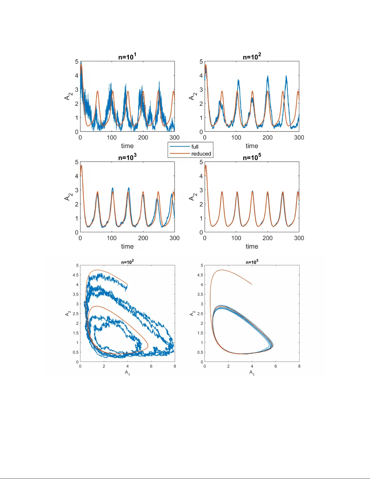
STOCHASTIC A VERA GING AND ST A TISTICAL INFERENCE OF GL YCOL YTIC P A THW A Y ARN AB GANGUL Y AND HYE-WON KANG A B S T R AC T . Many biological processes e xhibit oscillatory behavior . Among these, glycolytic oscillations have been extensiv ely studied due to their well-characterized biochemical reaction networks. Howe ver , the complex- ity of these networks necessitates low-dimensional ordinary differential equation (ODE) models to identify core mechanisms and perform stability analysis. While pre vious studies proposed reduced ODE models, these were typically introduced from deterministic descriptions rather than the underlying stochastic dynamics, which more accurately represent discrete reaction events occurring at random times. In this paper, we dev elop a rig- orous probabilistic framework for deriving a reduced Othmer-Aldridge model of the glycolytic pathway from its stochastic formulation. The full system is modeled as a multiscale continuous-time Markov chain with dif- ferent time and abundance scales. Under an appropriate scaling regime and specific structural conditions, we prov e that the dynamics of the slow components are approximated by a two-dimensional ODE. The proof is technically in volv ed due to the network’ s complexity and strong coupling between its components. W e further consider the problem of parameter estimation when observations are limited to the slow species: fructose-6- phosphate and ADP . The reduced system yields a tractable loss function depending solely on these variables. W e prov e that the resulting estimators are statistically consistent when the data originate from the full stochas- tic reaction network. T ogether , these results provide a mathematically rigorous framework linking stochastic biochemical reaction networks, reduced deterministic dynamics, and statistically reliable parameter estimation. 1. I N T RO D U C T I O N . Understanding oscillatory systems is fundamental in biology , as many biological processes exhibit rh yth- mic behaviors across multiple scales. At the molecular level, certain gene expression dynamics induce circadian oscillations in mRN A and protein concentrations. At the subcellular lev el, metabolites display oscillatory behavior through alternating activ ation and inhibition of enzymes. On a larger scale, some mi- crobial populations, such as yeast, exhibit collectiv e population rhythms arising from the synchronization of individual cellular oscillations. Pre vious studies hav e re vealed that nonlinear interactions and feedback mechanisms are key components required to generate and sustain such oscillations [ 19 , 12 ]. Ne vertheless, further research is needed to elucidate these oscillatory behaviors across complex biological systems span- ning genetics, physiology , and ecology . Among these oscillatory systems, glycolytic oscillations have been extensi vely studied using dynamical models because the underlying biochemical reaction networks are relatively well characterized. The classi- cal Higgins and Selko v models [ 14 , 24 ], formulated as systems of ordinary differential equations (ODEs), describe glycolytic oscillations using two variables—substrate and product—interacting through nonlinear feedback. Building on Higgins’ general framew ork, Othmer and Aldridge proposed ODE-based models to study oscillations and synchronization at the population level [ 20 ]. Ho wev er , the deriv ation of these two-v ariable models was largely heuristic and lacked rigorous mathematical justification. 2020 Mathematics Subject Classification. 60F17, 60H30, 60J28, 60J74, 62F12, 92-10. K e y wor ds and phrases. Stochastic Reaction Networks, Glycolytic Pathway , Multiscale systems, Stochastic A veraging, QSSA. A. Ganguly is the corresponding author . Research of A. Ganguly is supported in part byNSF DMS - 2246815 and Simons Foundation (via Tra vel Support for Mathematicians). The authors gratefully acknowledge the organizers of the W orkshop on Chemical Reaction Network Theory held at POSTECH (Pohang University of Science and T echnology) in the Republic of K orea in July 2024, where this project was initiated. 1 2 Deri ving low-dimensional ODE models remains a powerful approach for understanding oscillatory dy- namics in biological systems. Such models allow researchers to identify essential mechanisms responsible for oscillatory beha vior and to perform analytical in vestigations using tools such as stability and bifurcation analysis. These analyses help determine the existence of limit cycles and the conditions under which oscil- lations arise. Moreov er , simple ODE models enable systematic exploration of oscillation properties such as period and amplitude. T ogether , these theoretical and numerical analyses contrib ute to a deeper understand- ing of biological oscillations. Ho wev er, to ensure reliability , a rigorous deriv ation of such reduced models is essential. One common method for deriving reduced ODE models from complex biochemical systems is singular perturbation analysis. By identifying fast and slo w v ariables, one separates time scales and deri ves an approximate lower -dimensional system defined on a slo w manifold. This approach, often referred to as the quasi-steady-state approximation (QSSA), assumes that fast variables rapidly con ver ge to quasi-equilibrium and can therefore be expressed as functions of the slo w variables [ 23 ]. While this methodology has been widely successful, its application to oscillatory systems is delicate. In particular , it is known that a full deterministic model without oscillations may yield a reduced system e xhibiting oscillations, and con versely , oscillatory behavior in the full model may disappear after reduction [ 5 , 16 ]. Since oscillations depend sensiti vely on nonlinear feedback structure and global phase-space geometry , time-scale reduction at the deterministic le vel can alter essential dynamical features. Moreov er , deterministic ODE descriptions themselves arise as approximations of underlying stochastic reaction networks. Biochemical systems ev olve through discrete reaction e vents occurring randomly in time, and their natural mathematical representation is a continuous-time Marko v chain (CTMC) model [ 10 , 1 ]. Deterministic mass-action equations emerge from such models under suitable scaling limits via law-of- large-numbers (LLN) arguments [ 17 ]. This observ ation suggests that model reduction can be performed at a more fundamental lev el by starting from the stochastic formulation rather than from a deterministic system that is already an approximation. Moti vated by this perspecti ve, this paper takes a probabilistic approach. The primary contribution is twofold. First, we establish a LLN Theorem 3.1 showing that, under an appropriate multiscale scaling regime, the CTMC formulation of the glycolytic reaction network con verges to a two-dimensional ODE model describing the ev olution of the slo w species. In contrast to singular perturbation or QSSA-based reductions, where one begins with a deterministic ODE system and deri ves a lower -dimensional approxi- mation through formal time-scale separation, our deriv ation proceeds at the level of the stochastic reaction network itself. The reduced ODE does not arise from a perturbativ e expansion of a pre-existing determin- istic model; rather , it emerges as a scaling limit in probability of the underlying jump process, in the same spirit as other LLNs in which deterministic mean-field equations arise as limits of stochastic particle systems in statistical physics. This approach provides a rigorous probabilistic foundation for the reduced dynamics and clarifies precisely under what scaling assumptions the lo w-dimensional ODE accurately captures the macroscopic beha vior of the biochemical system. The rigorous analysis yields structural insight into the multiscale structure of the glycolytic network, and specifies which combinations of microscopic parameters gov ern the ef fectiv e macroscopic dynamics. Second, we address statistical inference for the glycolytic pathway when observations are av ailable only for the slo w species fructose-6-phosphate (F6P) and ADP (denoted by A 1 and A 2 ). In the full stochastic re- action netw ork, the high dimensionality , strong nonlinear coupling, and presence of unobserved fast species render direct likelihood-based or trajectory-based inference computationally prohibiti ve and statistically ill-posed. The reduced-order model, by contrast, yields a closed and low-dimensional dynamical system expressed solely in terms of the observed slow variables, thereby providing a tractable and well-defined loss function for parameter estimation. Our second main result, Theorem 4.1 , establishes statistical consistency of the estimators obtained by minimizing this loss function. Importantly , the observational data are assumed to be generated by the original multiscale CTMC dynamics rather than by the limiting ODE, reflecting the 3 fact that the latter is an approximation rather than the true data-generating mechanism. The LLN result, which rigorously connects the microscopic CTMC to the reduced ODE under a specified multiscale regime, plays a crucial role in the proof. While this scaling limit provides the essential link between the microscopic and reduced dynamics, establishing consistency of the estimators for the effecti ve parameters of the reduced model requires a substantially deeper argument. This result provides a mathematically justified framew ork for data-dri ven inference using the reduced model, which would otherwise be infeasible. Our LLN-result falls within the realm of stochastic av eraging. At a conceptual lev el, the overall strategy for proving stochastic av eraging is well-known and can be summarized in a couple of steps. One first typi- cally pro ves tightness of the slow component in a suitable function space (e.g., C ([0 , T ] , R d ) for continuous processes or D ([0 , T ] , R d ) for c ` adl ` ag processes) and tightness of the occupation measures associated with the fast component, viewed as measure-valued random variables. Tightness ensures the existence of limit points for the joint process. The final step is to identify these limit points and prove uniqueness for the limiting slo w dynamics, thereby characterizing the reduced model. This program has been implemented for generic continuous It ˆ o diffusion processes under ideal conditions, such as Lipschitz drift and diffusion coefficients and often weak coupling between slow and f ast components [ 13 , 21 , 22 , 7 , 8 ]. It has been formalized in [ 15 ] for equations arising from reaction systems (see also [ 4 ] for simpler classes of reaction systems). These works primarily adopt a generator-based approach building on [ 18 ], which pro vides a general frame work for stochastic a veraging of certain martingale problems. How- e ver , such results serve as a structural blueprint, rather than a turnkey solution: the principal mathematical challenge of course lies in ex ecuting the av eraging strategy for specific models. In the present case, the CTMC model of the glycolytic pathway is highly intricate (see Figure 1 ), in volving ten species and sixteen reactions that form a strongly coupled network of jump processes. The reaction rates span four distinct scales, O ( n − 1 ) , O (1) , O ( n 1 / 2 ) , and O ( n ) , while species abundances occur on three scales, O (1) , O ( n ) , and O ( n 2 ) . Here n denotes a scaling parameter that captures differences in species abundances and reaction speeds. Moreo ver , both slo w and fast reactions influence the dynamics of the slo w and fast components (see ( 2.7 ), ( 2.8 )). These features places our system outside the scope of standard stochastic av eraging frame works, and ev en if one were content with an abstract characterization of the limit — without seeking an explicit closed-form expression — the hypotheses of generic stochastic averaging theorems are not satisfied, and hence such results cannot be in voked to justify con ver gence. Thus, implementing the broad steps outlined abov e for this system is a delicate task and requires a careful examination of the specific network structure underlying the glycolytic pathway . In particular , establish- ing tightness of the occupation measures for the fast subsystem, together with controlling certain integrals in volving these measures, is challenging. Both are required at various points in the proofs and are compli- cated by the rapid fluctuations of AMP (denoted by A 3 ). Addressing these obstacles requires non-standard techniques, including delicate martingale estimates that exploit the specific structure of the network (see Proposition 3.1 ). In contrast to functional analytic techniques based on conv ergence of relev ant generators and semigroups [ 18 , 2 , 4 ], which are often difficult to employ for complex models like ours, our approach is probabilistic in nature relying on representation of the species-processes as solutions of stochastic differ - ential equations (SDEs) driv en by Poisson random measures (PRMs). In our opinion, this in fact provides more transparent insights into species dynamics and the interplay between fast and slo w reactions. Such SDE-based representations were previously used to mathematically justify popular total Quasi-Steady State Approximations (tQSSA) for Michaelis-Menten kinetics in a recent work of the first author , [ 9 ]. A further dif ficulty arises at the identification stage. In generic stochastic av eraging theorems, the limiting slo w equation is characterized in abstract form: the drift of the slow variable is expressed as an average of certain coefficients with respect to an in variant distribution of the fast process, which is assumed to be unique. Such an abstract characterization of the reduced model is clearly inadequate for practical purposes, 4 as it does not provide a tractable model for numerical simulation and parameter estimation. T o be usable, the limiting dynamics must be av ailable in explicit closed form. But, to this end, we note that the abstract averaging frame work is not ev en applicable in our setting. The reason is that, in our case, the equilibrium distribution of the fast subsystem, which satisfies a complex PDE, is neither av ailable in closed form nor guaranteed to be unique. As a result, one cannot simply apply a general stochastic av eraging theorem to justify the reduced equation. Instead, a more detailed analysis of the network structure is required to establish the relev ant ergodic properties and to demonstrate that, de- spite these obstacles, the limiting equation for the slo w species is both unique and explicitly computable, thereby yielding a concrete and computationally tractable reduced-order model suitable for both simulation and parameter estimation. Unlike earlier heuristic reductions of the complex glycolytic pathway relying on quasi-steady-state or partial equilibrium assumptions, our deriv ation provides a mathematically rigor- ous foundation of the Othmer–Aldridge model that not only retains the key oscillatory kinetics but also mathematically justifies its ef ficacy in statistical inference from data on the slo w species. The rest of the paper is organized as follows. In Section 2 , we introduce the stochastic model of the gly- colytic pathway and formulate its pathwise representation as a system of SDEs driv en by Poisson random measures. The main stochastic av eraging result is established in Section 3 . W e also discuss the resulting reduced-order system and present numerical simulations comparing it with the full CTMC model. Sec- tion Section 4 is de vot ed to parameter estimation based on the reduced model. Our primary result in this section is the consistency of the proposed estimators. Numerical experiments v alidating accuracy of the estimators are also presented. 1.1. Notational conv entions. • The space of continuous functions from E to F will be denoted by C ( E , F ) with the subset C b ( E , F ) , C c ( E , F ) denoting the bounded, continuous and compactly supported continuous functions, respectiv ely . These spaces are equipped with their usual topologies. For T > 0 , the space C ([0 , T ] , F ) is a subset of D ([0 , T ] , F ) , the space of c ` adl ` ag functions from [0 , T ] to F . D ([0 , T ] , F ) will be equipped with the Skorokhod topology . • The σ -field generated by the Borel subsets of E will be denoted by B ( E ) . • M ( E ) will denote the space of finite (non-negati ve) measures on E equipped with the topology of weak con ver gence. For r > 0 , M r ( E ) ⊂ M ( E ) will denote the space of (non-negati ve) measures ν such that ν ( E ) = r . • The indicator function of a set A will be denoted by 1 A ( · ) , i.e., 1 A ( x ) = 1 if x ∈ A , and zero otherwise. • W e use Λ Leb to denote the Lebesgue measure on R . • For a c ` adl ` ag function f , we denote the left-hand limit of the function f at t by f ( t − ) . • For u ∈ R d or Z d , ∥ u ∥ 1 = P d i =1 | u i | . • Other notations will be introduced when needed. 2. M A T H E M A T I C A L F R A M E W O R K A wide v ariety of simplified glycolytic pathways ha ve been studied to understand the oscillatory behavior observed in metabolic intermediates of glycolysis [ 14 , 24 , 20 ]. Among these, we focus on the enzyme- catalyzed reaction mechanism introduced by Othmer and Aldridge [ 20 ]. This mechanism consists of ten chemical species and sixteen reactions. W e denote by A 1 and A 2 fructose- 6-phosphate (F6P) and ADP , respectiv ely; A 3 and A 4 represent AMP and A TP . The v ariables E 1 and E ∗ 1 correspond to the low-acti vity and activ ated forms of phosphofructokinase-1 (PFK). The complex es formed between PFK abd F6P are denoted by E 1 A 1 and E ∗ 1 A 1 . In addition, E 2 denotes an enzyme responsible for ADP degradation, and E 2 A 2 denotes its complex with ADP . The full chemical reaction network is is presented in Figure 1 . 5 A 1 : F6P , A 2 : ADP , A 3 : AMP , A 4 : A TP E 1 : low activity PFK, E ∗ 1 : activated PFK E 2 : enzyme for ADP degradation E 1 + A 1 ∅ κ ( n ) 0 E 1 A 1 E 1 + A 2 κ ( n ) 1 κ ( n ) − 1 κ ( n ) 2 + A 3 + A 3 E ∗ 1 + A 1 E ∗ 1 A 1 E ∗ 1 + A 2 κ ( n ) − 7 κ ( n ) 7 κ ( n ) 7 κ ( n ) − 7 κ ( n ) 3 κ ( n ) − 3 κ ( n ) 4 E 2 + A 2 E 2 A 2 E 2 + Product κ ( n ) 5 κ ( n ) − 5 κ ( n ) 6 A 2 + A 2 A 3 + A 4 κ ( n ) 8 κ ( n ) − 8 F I G U R E 1 . Glycolytic Pathway This mechanism pro vides a simplified description of the glycolytic pathw ay , focusing on the rate-limiting phosphorylation of F6P ( A 1 ) by A TP , which produces fructose-1,6-bisphosphate and ADP ( A 2 ). PFK cat- alyzes this step and exhibits either low ( E 1 ) or high ( E ∗ 1 ) activity depending on the cellular AMP concen- tration. ADP ( A 2 ) participates in downstream reactions of glycolysis, modeled here as an ADP-degradation process catalyzed by E 2 . AMP ( A 3 ) binds to both free and substrate-bound lo w-activity PFKs ( E 1 and E 1 A 1 ), con verting them into their acti vated forms ( E ∗ 1 and E ∗ 1 A 1 ). Moreov er , AMP and A TP interconv ert with ADP through a re versible reaction. In their study , Othmer and Aldridge [ 20 ] deriv ed a two-v ariable reduction of the full mechanism under the follo wing assumptions: (i) the enzyme-substrate complex es E 1 A 1 , E ∗ 1 A 1 , and E 2 A 2 satisfy a quasi- steady-state approximations; (ii) the activ ation reactions in volving E 1 and E 1 A 1 are in partial equilibrium; and (iii) the intercon version of A 4 is also in partial equilibrium. The resulting reduced dynamics for the concentrations of A 1 and A 2 take the form dx dt = k − ¯ f ( x, y ) , dy dt = ¯ f ( x, y ) − ¯ g ( y ) (2.1) where x and y denote the concentrations of F6P and ADP , respectively . Howe ver , the deriv ation of this reduced model was presented only heuristically , and conditions under which the approximation captures the oscillatory behavior of the full reaction netw ork hav e not been rigorouly analyzed. The first part of the paper will focus on how to rigorously deriv e a reduced-order ODE model of the form ( 2.1 ) starting from a Markov chain formulation of the reaction system in Figure 1 in a suitable scaling regime. 6 2.1. Stochastic Description. For each n ⩾ 1 , viewed as a scaling parameter that encodes differences in species abundance and reaction speeds, we denote by X ( n ) the stochastic process representing the species vector , X ( n ) =  X ( n ) A 1 , X ( n ) A 1 , X ( n ) A 3 , X ( n ) A 4 , X ( n ) E 1 , X ( n ) E ∗ 1 , X ( n ) E 1 A 1 , X ( n ) E ∗ 1 A 1 , X ( n ) E 2 , X ( n ) E 2 A 2  . Denote the reaction index set as R = { 0 , ± 1 , 2 , ± 3 , 4 , ± 5 , 6 , ± 7 , ± 7 ′ , ± 8 } . For each k ∈ R , define an increasing pure jump process R ( n ) k by R ( n ) k ( t ) = Z [0 , ∞ ) × [0 ,t ] 1 [0 ,λ ( n ) k ( X ( n ) ( s − ))] ( u ) ξ k ( du × ds ) , (2.2) where the ξ k are Poisson random measures (PRMs) on [0 , ∞ ) × [0 , ∞ ) with mean measure as product of Lebesgue measures, Λ Leb ⊗ Λ Leb . R ( n ) k ( t ) is the number of occurrences of the k -th reaction with propensity functions λ ( n ) k in [0 , t ] . The propensity functions λ ( n ) k are defined as follo ws: λ ( n ) 0 ( x ) ≡ κ ( n ) 0 , and λ ( n ) 1 ( x ) = κ ( n ) 1 x E 1 x A 1 , λ ( n ) − 1 ( x ) = κ ( n ) − 1 x E 1 A 1 , λ ( n ) 2 ( x ) = κ ( n ) 2 x E 1 A 1 , λ ( n ) 3 ( x ) = κ ( n ) 3 x E ∗ 1 x A 1 , λ ( n ) − 3 ( x ) = κ ( n ) − 3 x E ∗ 1 A 1 , λ ( n ) 4 ( x ) = κ ( n ) 4 x E ∗ 1 A 1 , λ ( n ) 5 ( x ) = κ ( n ) 5 x E 2 x A 2 , λ ( n ) − 5 ( x ) = κ ( n ) − 5 x E 2 A 2 , λ ( n ) 6 ( x ) = κ ( n ) 6 x E 2 A 2 , λ ( n ) 7 ( x ) = κ ( n ) 7 x E 1 x A 3 , λ ( n ) − 7 ( x ) = κ ( n ) − 7 x E ∗ 1 , λ ( n ) 7 ′ ( x ) = κ ( n ) 7 x E 1 A 1 x A 3 , λ ( n ) − 7 ′ ( x ) = κ ( n ) − 7 x E ∗ 1 A 1 , λ ( n ) 8 ( x ) = κ ( n ) 8 x A 2 ( x A 2 − 1) , λ ( n ) − 8 ( x ) = κ ( n ) − 8 x A 3 x A 4 . (2.3) Here, for con venience of tracking, a typical state x ∈ Z 10 ⩾ 0 will be denoted as x = ( x A 1 , x A 2 , x A 3 , x A 4 , x E 1 , x E ∗ 1 , x E 1 A 1 , x E ∗ 1 A 1 , x E 2 , x E 2 A 2 ) instead of the more typical x = ( x 1 , x 2 , . . . , x 10 ) . It is no w clear from the reaction system in Figure 1 that the trajectories of X ( n ) are gi ven by X ( n ) A 1 ( t ) = X ( n ) A 1 (0) + R ( n ) 0 ( t ) − R ( n ) 1 ( t ) + R ( n ) − 1 ( t ) − R ( n ) 3 ( t ) + R ( n ) − 3 ( t ) , X ( n ) A 2 ( t ) = X ( n ) A 2 (0) + R ( n ) 2 ( t ) + R ( n ) 4 ( t ) − R ( n ) 5 ( t ) + R ( n ) − 5 ( t ) − 2 R ( n ) 8 ( t ) + 2 R ( n ) − 8 ( t ) , X ( n ) A 3 ( t ) = X ( n ) A 3 (0) − R ( n ) 7 ( t ) + R ( n ) − 7 ( t ) − R ( n ) 7 ′ ( t ) + R ( n ) − 7 ′ ( t ) + R ( n ) 8 ( t ) − R ( n ) − 8 ( t ) , X ( n ) A 4 ( t ) = X ( n ) A 4 (0) + R ( n ) 8 ( t ) − R ( n ) − 8 ( t ) , X ( n ) E 1 ( t ) = X ( n ) E 1 (0) − R ( n ) 1 ( t ) + R ( n ) − 1 ( t ) + R ( n ) 2 ( t ) − R ( n ) 7 ( t ) + R ( n ) − 7 ( t ) , X ( n ) E ∗ 1 ( t ) = X ( n ) E ∗ 1 (0) − R ( n ) 3 ( t ) + R ( n ) − 3 ( t ) + R ( n ) 4 ( t ) + R ( n ) 7 ( t ) − R ( n ) − 7 ( t ) , X ( n ) E 1 A 1 ( t ) = X ( n ) E 1 A 1 (0) + R ( n ) 1 ( t ) − R ( n ) − 1 ( t ) − R ( n ) 2 ( t ) − R ( n ) 7 ′ ( t ) + R ( n ) − 7 ′ ( t ) , X ( n ) E ∗ 1 A 1 ( t ) = X ( n ) E ∗ 1 A 1 (0) + R ( n ) 3 ( t ) − R ( n ) − 3 ( t ) − R ( n ) 4 ( t ) + R ( n ) 7 ′ ( t ) − R ( n ) − 7 ′ ( t ) , X ( n ) E 2 ( t ) = X ( n ) E 2 (0) − R ( n ) 5 ( t ) + R ( n ) − 5 ( t ) + R ( n ) 6 ( t ) , X ( n ) E 2 A 2 ( t ) = X ( n ) E 2 A 2 (0) + R ( n ) 5 ( t ) − R ( n ) − 5 ( t ) − R ( n ) 6 ( t ) , (2.4) which constitutes a system of SDEs dri ven by Poisson random measures (PRM) written in inte gral form. In order to study the averaging phenomena, we consider the [0 , ∞ ) 10 -v alued scaled process vector Z ( n ) defined by Z ( n ) i ( t ) = n − α i X ( n ) i ( t ) , i ∈ { A 1 , A 2 , A 3 , A 4 , E 1 , E ∗ 1 , E 1 A 1 , E ∗ 1 A 1 , E 2 , E 2 A 2 } . (2.5) 7 The α i ∈ R are scaling exponents that describe variation in species abundance. W e also introduce the scaling exponents { β k } for reactions rates capturing variation in reaction speeds: κ k = n − β k κ ( n ) k , k = 0 , ± 1 , 2 , ± 3 , 4 , ± 5 , 6 , ± 7 , ± 8 . (2.6) As before, for con venience of tracking, a typical state z ∈ [0 , ∞ ) 10 of the process Z ( n ) will be denoted as z = ( z A 1 , z A 2 , z A 3 , z A 4 , z E 1 , z E ∗ 1 , z E 1 A 1 , z E ∗ 1 A 1 , z E 2 , z E 2 A 2 ) instead of the more typical z = ( z 1 , z 2 , . . . , z 10 ) . In this paper we operate in the follo wing scaling regime: α A 4 = 2 , α A 1 = α A 2 = 1 , α A 3 = α E 1 = α E ∗ 1 = α E 1 A 1 = α E ∗ 1 A 1 = α E 2 = α E 2 A 2 = 0 β 0 = β − 1 = β 2 = β − 3 = β 4 = β − 5 = β 6 = 1 , β 7 = β − 7 = 1 2 , β 1 = β 3 = β 5 = 0 , β 8 = β − 8 = − 1 . (2.7) W ith the above choice of the scaling parameters, the scaled process Z ( n ) satisfies the following system of equations: Z ( n ) A 1 ( t ) = Z ( n ) A 1 (0) + n − 1 h R ( n ) 0 ( t ) − R ( n ) 1 ( t ) + R ( n ) − 1 ( t ) − R ( n ) 3 ( t ) + R ( n ) − 3 ( t ) i , Z ( n ) A 2 ( t ) = Z ( n ) A 2 (0) + n − 1 h R ( n ) 2 ( t ) + R ( n ) 4 ( t ) − R ( n ) 5 ( t ) + R ( n ) − 5 ( t ) − 2 R ( n ) 8 ( t ) + 2 R ( n ) − 8 ( t ) i , Z ( n ) A 3 ( t ) = Z ( n ) A 3 (0) − R ( n ) 7 ( t ) + R ( n ) − 7 ( t ) − R ( n ) 7 ′ ( t ) + R ( n ) − 7 ′ ( t ) + R ( n ) 8 ( t ) − R ( n ) − 8 ( t ) , Z ( n ) A 4 ( t ) = Z ( n ) A 4 (0) + n − 2 h R ( n ) 8 ( t ) − R ( n ) − 8 ( t ) i , Z ( n ) E 1 ( t ) = Z ( n ) E 1 (0) − R ( n ) 1 ( t ) + R ( n ) − 1 ( t ) + R ( n ) 2 ( t ) − R ( n ) 7 ( t ) + R ( n ) − 7 ( t ) , Z ( n ) E ∗ 1 ( t ) = Z ( n ) E ∗ 1 (0) − R ( n ) 3 ( t ) + R ( n ) − 3 ( t ) + R ( n ) 4 ( t ) + R ( n ) 7 ( t ) − R ( n ) − 7 ( t ) , Z ( n ) E 1 A 1 ( t ) = Z ( n ) E 1 A 1 (0) + R ( n ) 1 ( t ) − R ( n ) − 1 ( t ) − R ( n ) 2 ( t ) − R ( n ) 7 ′ ( t ) + R ( n ) − 7 ′ ( t ) , Z ( n ) E ∗ 1 A 1 ( t ) = Z ( n ) E ∗ 1 A 1 (0) + R ( n ) 3 ( t ) − R ( n ) − 3 ( t ) − R ( n ) 4 ( t ) + R ( n ) 7 ′ ( t ) − R ( n ) − 7 ′ ( t ) , Z ( n ) E 2 ( t ) = Z ( n ) E 2 (0) − R ( n ) 5 ( t ) + R ( n ) − 5 ( t ) + R ( n ) 6 ( t ) , Z ( n ) E 2 A 2 ( t ) = Z ( n ) E 2 A 2 (0) + R ( n ) 5 ( t ) − R ( n ) − 5 ( t ) − R ( n ) 6 ( t ) . (2.8) Conservation Laws: Notice that the following conserv ation laws hold: for all t ⩾ 0 , Z ( n ) E 1 ( t ) + Z ( n ) E 1 A 1 ( t ) + Z ( n ) E ∗ 1 ( t ) + Z ( n ) E ∗ 1 A 1 ( t ) ≡ J ( n ) 1 , Z ( n ) E 2 ( t ) + Z ( n ) E 2 A 2 ( t ) ≡ J ( n ) 2 . (2.9) Denote the species index-sets S and F by S = { A 1 , A 2 , A 4 } , F = { A 3 , E 1 , E ∗ 1 , E 1 A 1 , E ∗ 1 A 1 , E 2 , E 2 A 2 } , (2.10) and write Z ( n ) = ( Z ( n ) S , Z ( n ) F ) , where Z ( n ) S def =  Z ( n ) A 1 , Z ( n ) A 2 , Z ( n ) A 4  , Z ( n ) F def =  Z ( n ) A 3 , Z ( n ) E 1 , Z ( n ) E ∗ 1 , Z ( n ) E 1 A 1 , Z ( n ) E ∗ 1 A 1 , Z ( n ) E 2 , Z ( n ) E 2 A 2  . (2.11) When necessary , a typical state z ∈ [0 , ∞ ) 10 of Z ( n ) = ( Z ( n ) S , Z ( n ) F ) will be split as z = ( z S , z F ) with z S = ( z A 1 , z A 2 , z A 4 ) ∈ [0 , ∞ ) 3 and z F = ( z A 3 , z E 1 , z E ∗ 1 , z E 1 A 1 , z E ∗ 1 A 1 , z E 2 , z E 2 A 2 ) ∈ [0 , ∞ ) 7 . In the scaling regime defined by ( 2.7 ), Z ( n ) F will be the fast process and Z ( n ) S will be the slow process. Our primary goal is to show that as Z ( n ) S n →∞ − → Z S in D ([0 , T ] , [0 , ∞ ) 3 ) where Z S is the solution of a possibly random ODE. W e present this stochastic av eraging result in the next section. 8 3. S T O C H A S T I C A V E R A G I N G W e start with the necessary assumptions for the main con ver gence result to hold. Assumption 3.1. The following conditions hold. (a) sup n E ∥ Z ( n ) (0) ∥ 1 < ∞ ; (b) sup n E h ( J ( n ) 1 ) 2 i ∨ sup n E h ( J ( n ) 2 ) 2 i < ∞ . (c) • for some random variables J 1 , J 2 , Z A 1 (0) , Z A 2 (0) and Z A 4 (0) , as n → ∞ ,  J ( n ) 1 , J ( n ) 2 , Z ( n ) A 1 (0) , Z ( n ) A 2 (0) , Z ( n ) A 4 (0)  P − →  J 1 , J 2 , Z A 1 (0) , Z A 2 (0) , Z A 4 (0)  ; • Z A 4 (0) > δ 0 a.s. for some δ 0 > 0 . • n n − 1  Z ( n ) A 3 (0)  p o is tight for some p > 2 . The first step to prov e the con ver gence of the slow process Z ( n ) S is to establish its tightness in D ([0 , T ] , [0 , ∞ ) 3 ) . T o analyze the rapid movement of the f ast process Z ( n ) F , we introduce its measure Γ ( n ) F as Γ ( n ) F ( A × [0 , t ]) = Z t 0 1 A ( Z ( n ) F ( s )) d s, A ⊂ [0 , ∞ ) 7 . Notice that Γ ( n ) F is a random measure taking values in M T ([0 , ∞ ) 7 × [0 , T ]) (see definition in Notational con ventions in Introduction) and Γ ( n ) F ([0 , ∞ ) 7 × [0 , t ]) = t for any t ∈ [0 , T ] . The following proposition establishes the necessary tightness of (Γ ( n ) F , Z ( n ) S ) . Proposition 3.1. Suppose that Assumption 3.1 holds. Then for any T > 0 , the sequence (Γ ( n ) F , Z ( n ) S ) is r elatively compact as M T ([0 , ∞ ) 7 × [0 , T ]) × D ([0 , T ] , [0 , ∞ ) 3 ) -valued random variables. Furthermor e, the limit points of Z ( n ) S ar e almost surely in C ([0 , T ] , [0 , ∞ ) 3 ) . W e are now ready to state our main con ver gence result. Theorem 3.1. Suppose that Assumption 3.1 holds. Then, as n → ∞ , Z ( n ) S ⇒ Z S = ( Z A 1 , Z A 2 , Z A 4 ) , wher e the path-space of of ( Z A 1 , Z A 2 ) is C ([0 , T ] , [0 , ∞ ) 2 ) , for P -a.a. ω ∈ Ω , Z A 4 ( t, ω ) ≡ Z A 4 (0) and ( Z A 1 ( · , ω ) , Z A 2 ( · , ω )) solves the (random) ODE d Z A 1 ( t ) d t = κ 0 − f ( Z A 1 ( t ) , Z A 2 ( t ) , Z A 4 (0)) d Z A 2 ( t ) d t = f ( Z A 1 ( t ) , Z A 2 ( t ) , Z A 4 (0)) − g ( Z A 2 ( t )) Z A 4 ( t ) ≡ Z A 4 (0) (3.1) with initial condition Z S (0 , ω ) = ( Z A 1 (0 , ω ) , Z A 2 (0 , ω ) , Z A 4 (0 , ω )) at time zer o. Her e f ( z A 1 , z A 2 , z A 4 ) = 1 K 1 z A 4 + z 2 A 2 " J • 1 K 1 z A 1 z A 4 K M 1 + z A 1 + J ⋆ 1 z A 1 z 2 A 2 K ⋆ M 1 + z A 1 # , g ( z A 2 ) = J • 2 z A 2 K M 2 + z A 2 , (3.2) and K 1 ≡ κ − 7 κ − 8 κ 7 κ 8 , K M 1 ≡ κ − 1 + κ 2 k 1 , K ⋆ M 1 ≡ κ − 3 + κ 4 κ 3 , K M 2 ≡ κ − 5 + κ 6 κ 5 J • 1 ≡ κ 2 J 1 , J ⋆ 1 ≡ κ 4 J 1 , J • 2 ≡ κ 6 J 2 . (3.3) 9 In particular , if Z S (0) , J 1 and J 2 ar e deterministic (non-random), then Z S is deterministic, and hence as n → ∞ , Z ( n ) S P − → Z S in C ([0 , T ] , [0 , ∞ )) , that is, sup t ⩽ T ∥ Z ( n ) S ( t ) − Z S ( t ) ∥ P − → 0 . W e now tow ard the proofs of these results, which are technically in volved and require a number of delicate estimates relying on a careful analysis of the reaction network structure. T o this end, we first observe that the reaction-number process R ( n ) k defined by ( 2.2 ), and its ‘centered version’ ˜ R ( n ) k ( · ) def = Z [0 , ∞ ) × [0 , · ] 1 [0 ,λ ( n ) k ( X ( n ) ( s − ))] ( u ) ˜ ξ k ( du × ds ) = R ( n ) k ( · ) − Z · 0 λ ( n ) k ( X ( n ) ( s )) ds can be written in terms of the Z ( n ) process as follo ws: (3.4)  R ( n ) k ( t ) , ˜ R ( n ) k ( t )  =               ξ 0  nκ 0 t  , ˜ ξ 0  nκ 0 t   , k = 0 , Z [0 , ∞ ) × [0 ,t ] 1 [0 ,nλ k ( Z ( n ) ( s − ))] ( u )  ξ k ( du × ds ) , ˜ ξ k ( du × ds )  , k = ± 1 , 2 , ± 3 , 4 , ± 5 , 6 , ± 8 , Z [0 , ∞ ) × [0 ,t ] 1 [0 ,n 1 / 2 λ k ( Z ( n ) ( s − ))] ( u )  ξ k ( du × ds ) , ˜ ξ k ( du × ds )  , k = ± 7 , ± 7 ′ , where recall that for each k ∈ R , ξ k is the PRM on [0 , ∞ ) × [0 , ∞ ) with mean measure Λ Leb ⊗ Λ Leb , and ˜ ξ k defined by ˜ ξ k ( A × [0 , t ]) − Λ Leb ( A ) t is the corresponding compensated PRM. The λ k appearing in ( 3.4 ) represent ‘scaled’ propensities, and are defined as follo ws: λ 0 ( z ) ≡ κ 0 and λ 1 ( z ) = κ 1 z E 1 z A 1 , λ − 1 ( z ) = κ − 1 z E 1 A 1 , λ 2 ( z ) = κ 2 z E 1 A 1 , λ 3 ( z ) = κ 3 z E ∗ 1 z A 1 , λ − 3 ( z ) = κ − 3 z E ∗ 1 A 1 , λ 4 ( z ) = κ 4 z E ∗ 1 A 1 , λ 5 ( z ) = κ 5 z E 2 z A 2 , λ − 5 ( z ) = κ − 5 z E 2 A 2 , λ 6 ( z ) = κ 6 z E 2 A 2 , λ 7 ( z ) = κ 7 z E 1 z A 3 , λ − 7 ( z ) = κ − 7 z E ∗ 1 , λ 7 ′ ( z ) = κ 7 z E 1 A 1 z A 3 , λ − 7 ′ ( z ) = κ − 7 z E ∗ 1 A 1 , λ 8 ( z ) = κ 8 z A 2  z A 2 − n − 1  , λ − 8 ( z ) = κ − 8 z A 3 z A 4 . (3.5) For con venience, we introduce the follo wing notation: r ( n ) k ( t ) = Z t 0 λ k ( Z ( n ) ( s )) ds, k = 0 , ± 1 , 2 , ± 3 , 4 , ± 5 , 6 , ± 8 , ± 7 , ± 7 ′ . (3.6) Clearly , R ( n ) k =    ˜ R ( n ) k + n r ( n ) k , k = 0 , ± 1 , 2 , ± 3 , 4 , ± 5 , 6 , ± 8 , ˜ R ( n ) k + n 1 / 2 r ( n ) k , k = ± 7 , ± 7 ′ , (3.7) 10 and since each ˜ R ( n ) k is a martingale, E h R ( n ) k ( t ) i =    n E h r ( n ) k ( t ) i , k = ± 1 , 2 , ± 3 , 4 , ± 5 , 6 , ± 8 n 1 / 2 E h r ( n ) k ( t ) i , k = ± 7 , ± 7 ′ . E h ( R ( n ) k ( t )) 2 i =        E   n r ( n ) k ( t )  2 + n r ( n ) k ( t )  , k = ± 1 , 2 , ± 3 , 4 , ± 5 , 6 , ± 8 E   n 1 / 2 r ( n ) k ( t )  2 + n 1 / 2 r ( n ) k ( t )  , k = ± 7 , ± 7 ′ . (3.8) T o prove Proposition 3.1 , we begin with the following lemma, which provides the necessary moment estimates and establishes C -tightness (see Definition A.1 ) for some of the scaled reaction-count processes. Lemma 3.1. Under Assumption 3.1 , the following assertions hold: (i) F or k = 0 , − 1 , 2 , − 3 , 4 , − 5 , 6 , − 7 , − 7 ′ , sup n E h ( r ( n ) k ( T )) 2 i < ∞ and the sequences of pr ocesses { r ( n ) k } ar e tight in C ([0 , T ] , [0 , ∞ )) . F or k = 0 , − 1 , 2 , − 3 , 4 , − 5 , 6 , the sequences of pr ocesses { n − 1 R ( n ) k } , and for k = − 7 , − 7 ′ , { n − 1 / 2 R ( n ) k } are C -tight in D ([0 , T ] , [0 , ∞ )) . (ii) sup n E  sup t ⩽ T  Z ( n ) A 1 ( t )  2  ∨ sup n E  sup t ⩽ T  Z ( n ) A 2 ( t )  2  < ∞ . Furthermore , sup n E  sup t ⩽ T  Z ( n ) A 3 ( t ) /n  2  < ∞ . (iii) F or k = 1 , 3 , 5 , 8 , sup n E h r ( n ) k ( T ) i < ∞ , the sequences of pr ocesses n r ( n ) k o ar e tight in C ([0 , T ] , [0 , ∞ )) , and n n − 1 R ( n ) k o ar e C -tight in D ([0 , T ] , [0 , ∞ )) . (iv) The sequence of pr ocesses n n − 1 / 2 ( R ( n ) 7 + R ( n ) 7 ′ ) o is C -tight in D ([0 , T ] , [0 , ∞ )) . Furthermore , sup n E   r ( n ) 7 ( T )  2  ∨ sup n E   r ( n ) 7 ′ ( T )  2  < ∞ , sup n E h r ( n ) − 8 ( T ) i < ∞ . (3.9) (v) E  sup t ⩽ T | Z ( n ) A 4 ( t ) − Z ( n ) A 4 (0) |  → 0 , and sup t ⩽ T | Z ( n ) A 4 ( t ) − Z A 4 (0) | P − → 0 as n → ∞ Pr oof. (i) W e show tightness of r ( n ) 2 and { n − 1 R ( n ) 2 } . The tightness of other processes follow similarly . Since sup s ⩽ T Z ( n ) E 1 A 1 ( s ) ⩽ J ( n ) 1 , and sup n E h ( J ( n ) 1 ) 2 i < ∞ , it follows that sup n E h ( r ( n ) 2 ( T )) 2 i ⩽ sup n E h ( J ( n ) 1 ) 2 i κ 2 2 T 2 < ∞ . In particular , { sup t ⩽ T r ( n ) 2 ( t ) ≡ r ( n ) 2 ( T ) } is tight, and the tightness of the process { r ( n ) 2 } in C ([0 , T ] , R ) follo ws from Lemma A.1 . Next write (c.f. ( 3.7 )) n − 1 R ( n ) 2 ( t ) = n − 1 ˜ R ( n ) 2 ( t ) + r ( n ) 2 ( t ) where recall that ˜ R ( n ) 2 , defined by ˜ R ( n ) 2 ( t ) = R ( n ) 2 ( t ) − n r ( n ) 2 ( t ) = R [0 , ∞ ) × [0 ,t ] 1 [0 ,nκ 2 Z N E 1 A 1 ( s )] ( u ) ˜ ξ 2 ( du × ds ) , is a zero-mean martingale. The C -tightness of { n − 1 R ( n ) 2 } will follo w once we show that n − 1 ˜ R ( n ) 2 P − → 0 in D ([0 , T ] , R ) . In fact we sho w the following stronger statement: as n → ∞ , n − 1 sup t ⩽ T | ˜ R ( n ) 2 ( t ) | → 0 in L 2 (Ω , P ) . T o this end, observe that ⟨ n − 1 ˜ R ( n ) 2 ⟩ , the predictable quadratic v ariation of n − 1 ˜ R ( n ) 2 , satisfies ⟨ n − 1 ˜ R ( n ) 2 ⟩ t = n − 2 Z t 0 nκ 2 Z ( n ) E 1 A 1 ( s ) ds ⩽ n − 1 J ( n ) 1 T . 11 By Burkholder-Da vis-Gundy (BDG) inequality and the assumption on { J ( n ) 1 } , it follo ws that ⟨ n − 1 ˜ R ( n ) 2 ⟩ T → 0 in L 2 (Ω , P ) as n → ∞ , E  sup t ⩽ T | n − 1 ˜ R ( n ) 2 ( t ) | 2  ⩽ B 2 E ⟨ n − 1 ˜ R ( n ) 2 ⟩ T n →∞ − → 0 . (3.10) where B 2 is the Burkholder’ s constant for exponent 2. (ii) Notice that 0 ⩽ Z ( n ) A 1 ( t ) ⩽ Z ( n ) A 1 (0) + n − 1 h R ( n ) 0 ( t ) + R ( n ) − 1 ( t ) + R ( n ) − 3 ( t ) i , (3.11) and Z ( n ) A 2 ( t ) + 2 n − 1 Z ( n ) A 3 ( t ) = Z ( n ) A 2 (0) + 2 n − 1 Z ( n ) A 3 (0) + n − 1 h R ( n ) 2 ( t ) + R ( n ) 4 ( t ) − R ( n ) 5 ( t ) + R ( n ) − 5 ( t ) − 2 R ( n ) 8 ( t ) + 2 R ( n ) − 8 ( t ) i + 2 n − 1 h − R ( n ) 7 ( t ) + R ( n ) − 7 ( t ) − R ( n ) 7 ′ ( t ) + R ( n ) − 7 ′ ( t ) + R ( n ) 8 ( t ) − R ( n ) − 8 ( t ) i = Z ( n ) A 2 (0) + 2 n − 1 Z ( n ) A 3 (0) + n − 1 h R ( n ) 2 ( t ) + R ( n ) 4 ( t ) − R ( n ) 5 ( t ) + R ( n ) − 5 ( t ) 2  − R ( n ) 7 ( t ) + R ( n ) − 7 ( t ) − R ( n ) 7 ′ ( t ) + R ( n ) − 7 ′ ( t )  i ⩽ Z ( n ) A 2 (0) + 2 n − 1 Z ( n ) A 3 (0) + n − 1 h R ( n ) 2 ( t ) + R ( n ) 4 ( t ) + R ( n ) − 5 ( t ) + 2  R ( n ) − 7 ( t ) + R ( n ) − 7 ′ ( t )  i . (3.12) The assertion now follows by squaring both sides in ( 3.11 ) and ( 3.12 ), taking expectations, noting that sup t ⩽ T R ( n ) k ( t ) = R ( n ) k ( T ) (since R ( n ) k is nondecreasing), and then applying ( 3.8 ) together with (i) . (iii) The proof follo ws from (i) , (ii) and Lemma A.1 . (i v) Notice that n − 1 / 2 ( R ( n ) 7 ( t ) + R ( n ) 7 ′ ( t )) = n − 1 / 2  Z ( n ) E 1 (0) + Z ( n ) E 1 A 1 (0) − Z ( n ) E 1 ( t ) − Z ( n ) E 1 A 1 ( t )  + n − 1 / 2 ( R ( n ) − 7 ( t ) + R ( n ) − 7 ′ ( t )) . (3.13) No w since J ( n ) 1 is tight, sup t ⩽ T n − 1 / 2    Z ( n ) E 1 (0) + Z ( n ) E 1 A 1 (0) − Z ( n ) E 1 ( t ) − Z ( n ) E 1 A 1 ( t )    ⩽ 2 n − 1 / 2 J ( n ) 1 P − → 0 as n → ∞ . Since we already prov ed n − 1 / 2 R ( n ) − 7 and n − 1 / 2 R ( n ) − 7 ′ are C -tight, it follows that n − 1 / 2 ( R ( n ) 7 + R ( n ) 7 ′ ) is C -tight in D ([0 , T ] , [0 , ∞ )) . No w squaring both sides of ( 3.13 ), taking expectations and using ( 3.8 ), we ha ve E h r ( n ) 7 ( T )  2 +  r ( n ) 7 ′ ( T )  2 i ⩽ 4  n − 1 E h ( J ( n ) 1 ) 2 i + E h r ( n ) − 7 ( T )  2 + n − 1 / 2 r ( n ) − 7 ( T ) i + E h r ( n ) − 7 ′ ( T )  2 + n − 1 / 2 r ( n ) − 7 ′ ( T ) i , (3.14) which establishes the first inequality in ( 3.9 ), because of (i) and Assumption 3.1 - (a) . Next, notice that from the equation of Z ( n ) A 3 in ( 2.8 ), R ( n ) − 8 ( t ) ⩽ Z ( n ) A 3 (0) + R ( n ) − 7 ( t ) + R ( n ) − 7 ′ ( t ) + R ( n ) 8 ( t ) . 12 T aking expectation and di viding by n we get E ( r ( n ) − 8 ( T )) ⩽ n − 1 E ( Z ( n ) A 3 (0)) + n − 1 / 2 E ( r ( n ) − 7 ( T )) + n − 1 / 2 E ( r ( n ) − 7 ′ ( T )) + E ( r ( n ) 8 ( T )) . It no w follows from (i) , (iii) and Assumption 3.1 - (a) that the second inequality in ( 3.9 ) holds. (v) From the equation of Z ( n ) A 4 in ( 2.8 ), and using (iii) and (i v) , we obtain E  sup t ⩽ T | Z ( n ) A 4 ( t ) − Z ( n ) A 4 (0) |  ⩽ n − 1 E  r ( n ) 8 ( T ) + r ( n ) − 8 ( T )  n →∞ − → 0 . The second con vergence is immediate from Assumption 3.1 : (c) . □ Lemma 3.2. Under Assumption 3.1 , the sequence of random variables  Z T 0 Z ( n ) A 3 ( s ) ds  is tight. Pr oof. T o prove the assertion, we need to show that for any ϵ > 0 , there exists a K 1 ≡ K 1 ( ε ) and N 0 = N 0 ( ε ) such that for all n ⩾ N 0 ( ε ) P n ( K 1 ( ϵ )) def = P  Z T 0 Z ( n ) A 3 ( s ) ds ⩾ K 1 ( ε )  ⩽ ϵ. (3.15) Since sup n E  R T 0 Z ( n ) A 3 ( s ) Z ( n ) A 4 ( s ) ds  < ∞ by ( 3.9 ), by Markov inequality , choose K 1 ( ϵ ) such that P  2 δ 0 Z T 0 Z ( n ) A 3 ( s ) Z ( n ) A 4 ( s ) ds ⩾ K 1 ( ϵ )  ⩽ ϵ/ 3 , (3.16) where δ 0 is as in Assumption 3.1 - (c) . Now by Lemma 3.1 : (v) and the assumption Z ( n ) A 4 (0) P − → Z A 4 (0) , let N 0 be such that for all n ⩾ N 0 P  sup s ⩽ T | Z ( n ) A 4 ( s ) − Z ( n ) A 4 (0) | > δ 0 / 4  ∨ P  | Z ( n ) A 4 (0) − Z A 4 (0) | > δ 0 / 4  ⩽ ϵ/ 3 . Therefore, for all n ⩾ N 0 , P n ( K 1 ( ε )) ⩽ P  Z T 0 Z ( n ) A 3 ( s ) ds ⩾ K 1 ( ϵ ) , sup s ⩽ T | Z ( n ) A 4 ( s ) − Z ( n ) A 4 (0) | ⩽ δ 0 / 4  + ϵ/ 3 ⩽ P  Z T 0 Z ( n ) A 3 ( s ) ds ⩾ K 1 ( ϵ ) , sup s ⩽ T | Z ( n ) A 4 ( s ) − Z ( n ) A 4 (0) | ⩽ δ 0 / 4 , | Z ( n ) A 4 (0) − Z A 4 (0) | ⩽ δ 0 / 4  + 2 ϵ/ 3 No w writing R T 0 Z ( n ) A 3 ( s ) ds = R T 0 Z ( n ) A 3 ( s ) Z ( n ) A 4 ( s ) / Z ( n ) A 4 ( s ) ds , we see that on the event  sup s ⩽ T | Z ( n ) A 4 ( s ) − Z ( n ) A 4 (0) | ⩽ δ 0 / 4 , | Z ( n ) A 4 (0) − Z A 4 (0) | ⩽ δ 0 / 4  we hav e Z T 0 Z ( n ) A 3 ( s ) ds ⩽ 1 Z A 4 (0) − δ 0 / 2 Z T 0 Z ( n ) A 3 ( s ) Z ( n ) A 4 ( s ) ds ⩽ 2 δ 0 Z T 0 Z ( n ) A 3 ( s ) Z ( n ) A 4 ( s ) ds, where for the second inequality we have used the assumption that Z A 4 (0) ⩾ δ 0 a.s. Consequently , because of the choice of K 1 ( ϵ ) in ( 3.16 ), we have for all n ⩾ N 0 , P n ( K 1 ( ϵ )) ⩽ P  2 δ 0 Z T 0 Z ( n ) A 3 ( s ) Z ( n ) A 4 ( s ) ds ⩾ K 1 ( ϵ )  + 2 ϵ/ 3 ⩽ ϵ. □ 13 Proposition 3.2. Under Assumption 3.1 , the following hold: (i) the sequence of random variables n n − 1 sup t ⩽ T  Z ( n ) A 3 ( t )  p o is tight (where p is as in Assump- tion 3.1 : (c) ) (ii) the sequence of random variables  Z T 0 ( Z ( n ) A 3 ( s )) p ds  is tight. Remark 3.1. Pr oposition 3.2 : (i) implies that for any p 1 < p , n − 1 sup t ⩽ T  Z ( n ) A 3 ( t )  p 1 P − → 0 as n → ∞ . Pr oof of Pr oposition 3.2 . Notice that without loss of generality we can assume p to be positiv e integer v alued. W e will prov e (i) and (ii) by induction, that is, assuming that n n − 1 sup t ⩽ T  Z ( n ) A 3 ( t )  p ′ o and n R T 0 ( Z ( n ) A 3 ( s )) p ′ ds o are tight for any positiv e integer p ′ < p , we will show that (i) and (ii) hold. Observe that the case of p ′ = 1 follows from Lemma 3.1 : (ii) and Lemma 3.2 . By It ˆ o’ s lemma, ( Z ( n ) A 3 ( t )) p =( Z ( n ) A 3 (0)) p + ˆ R ( n,p ) − 7 ( t ) + ˆ R ( n,p ) − 7 ′ ( t ) + ˆ R ( n,p ) 8 ( t ) + ˆ R ( n,p ) 7 ( t ) + ˆ R ( n,p ) 7 ′ ( t ) + ˆ R ( n,p ) − 8 ( t ) , (3.17) where ˆ R ( n,p ) − 7 ( t ) = Z [0 , ∞ ) × [0 ,t ]  ( Z ( n ) A 3 ( s − ) + 1) p − ( Z ( n ) A 3 ( s − )) p  1 [0 ,n 1 / 2 κ − 7 Z ( n ) E ∗ 1 ( s − )] ( u ) ξ − 7 ( du × ds ) ˆ R ( n,p ) − 7 ′ ( t ) = Z [0 , ∞ ) × [0 ,t ]  ( Z ( n ) A 3 ( s − ) + 1) p − ( Z ( n ) A 3 ( s − )) p  1 [0 ,n 1 / 2 κ − 7 Z ( n ) E ∗ 1 A 1 ( s − )] ( u ) ξ − 7 ′ ( du × ds ) ˆ R ( n,p ) 8 ( t ) = Z [0 , ∞ ) × [0 ,t ]  ( Z ( n ) A 3 ( s − ) + 1) p − ( Z ( n ) A 3 ( s − )) p  1 [0 ,nκ 8 Z ( n ) A 2 ( s − )( Z ( n ) A 2 ( s − ) − n − 1 )] ( u ) ξ 8 ( du × ds ) ˆ R ( n,p ) 7 ( t ) = Z [0 , ∞ ) × [0 ,t ]  ( Z ( n ) A 3 ( s − ) − 1) p − ( Z ( n ) A 3 ( s − )) p  1 [0 ,n 1 / 2 κ 7 Z ( n ) E 1 ( s − ) Z ( n ) A 3 ( s − )] ( u ) ξ 7 ( du × ds ) ˆ R ( n,p ) 7 ′ ( t ) = Z [0 , ∞ ) × [0 ,t ]  ( Z ( n ) A 3 ( s − ) − 1) p − ( Z ( n ) A 3 ( s − )) p  1 [0 ,n 1 / 2 κ 7 Z ( n ) E 1 A 1 ( s − ) Z ( n ) A 3 ( s − )] ( u ) ξ 7 ′ ( du × ds ) ˆ R ( n,p ) − 8 ( t ) = Z [0 , ∞ ) × [0 ,t ]  ( Z ( n ) A 3 ( s − ) − 1) p − ( Z ( n ) A 3 ( s − )) p  1 [0 ,nκ − 8 Z ( n ) A 3 ( s − ) Z ( n ) A 4 ( s − )] ( u ) ξ − 8 ( du × ds ) . Binomial expansion sho ws that for y ⩾ 0 ( y + 1) p − y p = g ( p − 1) ( y ) , ( y − 1) p − ( y ) p ⩽ − py p − 1 + ˜ g ( p − 2) ( y ) ⩽ ˜ g ( p − 2) ( y ) , where g ( p − 1) ( · ) and ˜ g ( p − 2) ( · ) are nonnegati ve polynomials of degree p − 1 and p − 2 , respectiv ely . Thus, there is a constant C p such that 0 ⩽ g ( p − 1) ( y ) ⩽ C p (1 + y p − 1 ) , 0 ⩽ ˜ g ( p − 2) ( y ) ⩽ C p (1 + y p − 2 ) , y ⩾ 0 (3.18) Since the ξ k are non-negati ve measures, we ha ve sup t ⩽ T ( Z ( n ) A 3 ( t )) p ⩽ ( Z ( n ) A 3 (0)) p + G ( n,p − 1) − 7 ( T ) + G ( n,p − 1) − 7 ′ ( T ) + G ( n,p − 1) 8 ( T ) + ˜ G ( n,p − 2) 7 ( T ) + ˜ G ( n,p − 2) 7 ′ ( T ) + ˜ G ( n,p − 2) − 8 ( T ) , where G ( n,p − 1) k ( t ) = ( R [0 , ∞ ) × [0 ,t ] g ( p − 1) ( Z ( n ) A 3 ( s − )) 1 [0 ,n 1 / 2 λ k ( Z ( n ) ( s − ))] ( u ) ξ k ( du × ds ) , k = − 7 , − 7 ′ , R [0 , ∞ ) × [0 ,t ] g ( p − 1) ( Z ( n ) A 3 ( s − )) 1 [0 ,nλ k ( Z ( n ) ( s − ))] ( u ) ξ k ( du × ds ) , k = 8 , 14 ˜ G ( n,p − 2) k ( t ) = ( R [0 , ∞ ) × [0 ,t ] ˜ g ( p − 2) ( Z ( n ) A 3 ( s − )) 1 [0 ,n 1 / 2 λ k ( Z ( n ) ( s − ))] ( u ) ξ k ( du × ds ) , k = 7 , 7 ′ , R [0 , ∞ ) × [0 ,t ] ˜ g ( p − 2) ( Z ( n ) A 3 ( s − )) 1 [0 ,nλ k ( Z ( n ) ( s − ))] ( u ) ξ k ( du × ds ) , k = − 8 . The assertion (i) for exponent p follows once we show for k = − 7 , − 7 ′ , 8 , the sequences { n − 1 G ( n,p − 1) k ( T ) } are tight and for k = 7 , 7 ′ , − 8 , the sequences { n − 1 ˜ G ( n,p − 2) k ( T ) } are tight. W e will sho w this for the case of k = 8 ; that is, we show { n − 1 G ( n,p − 1) 8 ( T ) } is tight. The proofs for the others follow similarly and are actually simpler . T o this end, write G ( n,p − 1) 8 ( t ) = γ ( n,p − 1) 8 ( t ) + M ( n,p − 1) 8 ( t ) , where γ ( n,p − 1) 8 ( t ) = n Z t 0 g ( p − 1) ( Z ( n ) A 3 ( s )) λ k ( Z ( n ) ( s )) ds = nκ 8 Z t 0 g ( p − 1) ( Z ( n ) A 3 ( s )) Z ( n ) A 2 ( s )( Z ( n ) A 2 ( s ) − n − 1 ) ds, and the martingale, M ( n,p − 1) 8 , is defined by M ( n,p − 1) 8 ( t ) = Z [0 , ∞ ] × [0 ,T ] g ( p − 1) ( Z ( n ) A 3 ( s − )) 1 [0 ,nκ 8 Z ( n ) A 2 ( s − )( Z ( n ) A 2 ( s − ) − n − 1 )] ( u ) ˜ ξ 8 ( du × ds ) . Since  sup t ⩽ T  Z ( n ) A 2 ( t )  2  and n R T 0 ( Z ( n ) A 3 ( s ) p − 1 ds o are tight sequences of random variables by Lemma 3.1 : (ii) and the induction hypothesis, respecti vely , it follows that { n − 1 γ ( n,p − 1) 8 ( T ) } , satisfying the inequality n − 1 γ ( n,p − 1) 8 ( T ) ⩽ C p κ 8 sup t ⩽ T  Z ( n ) A 2 ( t )( Z ( n ) A 2 ( t ) + 1)  Z T 0  1 + Z ( n ) A 3 ( s )  p − 1 ds, is tight. Next notice that ⟨ M ( n,p − 1) 8 ⟩ , the predictable quadratic v ariation of the martingale b M ( n ) 8 , is gi ven by ⟨ M ( n,p − 1) 8 ⟩ t = nκ 8 Z t 0  g ( p − 1) ( Z ( n ) A 3 ( s ))  2 Z ( n ) A 2 ( s )( Z ( n ) A 2 ( s ) − n − 1 ) ds. Therefore, ⟨ n − 1 M ( n,p − 1) 8 ⟩ T = n − 2 ⟨ M ( n,p − 1) 8 ⟩ T ⩽ n − 1 C p κ 8 Z t 0  1 + Z ( n ) A 3 ( s )  2( p − 1) Z ( n ) A 2 ( s )( Z ( n ) A 2 ( s ) − n − 1 ) ds ⩽ C p κ 8  n − 1 sup t ⩽ T (1 + Z ( n ) A 3 ( s )) p − 1  sup t ⩽ T  Z ( n ) A 2 ( t )( Z ( n ) A 2 ( t ) + 1)  Z T 0  1 + Z ( n ) A 3 ( s )  p − 1 ds. Again since  sup t ⩽ T  Z ( n ) A 2 ( t )  2  , n n − 1 sup t ⩽ T ( Z ( n ) A 3 ( t )) p − 1 o and n R T 0 ( Z ( n ) A 3 ( s ) p − 1 ds o are tight by Lemma 3.1 : (ii) and induction-hypothesis, it follo ws that {⟨ n − 1 M ( n,p − 1) 8 ⟩ T } is tight. Hence, by Lemma A.3 { sup t ⩽ T | n − 1 M ( n,p − 1) 8 ( t ) |} is tight, and thus so is { n − 1 G ( n,p − 1) 8 ( T ) } . This establishes (i) for exponent p . T o prove (ii) , notice that ˆ R ( n,p ) − 8 ( t ) ⩽ − p Z t 0  Z ( n ) A 3 ( s − )  p − 1 1 [0 ,nκ − 8 Z ( n ) A 3 ( s − ) Z ( n ) A 4 ( s − )] ( u ) ξ − 8 ( du × ds ) + ˜ G ( n,p − 2) − 8 ( t ) and then rearranging ( 3.17 ) gi ves p Z t 0  Z ( n ) A 3 ( s )  p − 1 1 [0 ,nκ − 8 Z ( n ) A 3 ( s − ) Z ( n ) A 4 ( s − )] ( u ) ξ − 8 ( du × ds ) ⩽ ( Z ( n ) A 3 (0)) p + G ( n,p − 1) − 7 ( T ) + G ( n,p − 1) − 7 ′ ( T ) + G ( n,p − 1) 8 ( T ) + ˜ G ( n,p − 2) 7 ( T ) + ˜ G ( n,p − 2) 7 ′ ( T ) + ˜ G ( n,p − 2) − 8 ( T ) 15 which, by the results established while proving (i) , sho ws that the sequence  n − 1 Z t 0  Z ( n ) A 3 ( s − )  p − 1 1 [0 ,nκ − 8 Z ( n ) A 3 ( s − ) Z ( n ) A 4 ( s − )] ( u ) ξ − 8 ( du × ds )  is tight. Now observ e that κ − 8 Z t 0  Z ( n ) A 3 ( s )  p Z ( n ) A 4 ( s ) ds = − n − 1 ¯ M ( n,p − 1) − 8 ( t ) + n − 1 Z t 0  Z ( n ) A 3 ( s − )  p − 1 × 1 [0 ,nκ − 8 Z ( n ) A 3 ( s − ) Z ( n ) A 4 ( s − )] ( u ) ξ − 8 ( du × ds ) , (3.19) where the martingale term ¯ M ( n,p − 1) − 8 is defined by ¯ M ( n,p − 1) − 8 ( t ) = Z t 0  Z ( n ) A 3 ( s − )  p − 1 1 [0 ,nκ − 8 Z ( n ) A 3 ( s − ) Z ( n ) A 4 ( s − )] ( u ) ˜ ξ − 8 ( du × ds ) The quadratic v ariation ⟨ n − 1 ¯ M ( n,p − 1) − 8 ⟩ of the martingale n − 1 ¯ M ( n,p − 1) − 8 is gi ven by ⟨ n − 1 ¯ M ( n,p − 1) − 8 ⟩ t = n − 1 κ − 8 Z t 0 ( Z ( n ) A 3 ( s )) 2 p − 1 Z ( n ) A 4 ( s ) ds ⩽ κ − 8  n − 1 sup s ⩽ t ( Z ( n ) A 3 ( s )) p  sup s ⩽ t Z ( n ) A 4 ( s ) Z t 0  Z ( n ) A 3 ( s )  p − 1 ds. Since { sup s ⩽ t Z ( n ) A 4 ( s ) } and { n − 1 sup s ⩽ t ( Z ( n ) A 3 ( s )) p } are tight by Lemma 3.1 : (v) and just proven assertion (i) , and n R t 0  Z ( n ) A 3 ( s )  p − 1 ds o is tight by the induction hypothesis, {⟨ n − 1 ¯ M ( n,p − 1) − 8 ⟩ T } is tight, and so is n n − 1 sup t ⩽ T | ¯ M ( n,p − 1) − 8 ( t ) | o by Lemma A.3 . W e conclude from ( 3.19 ) that the sequence n R t 0  Z ( n ) A 3 ( s )  p Z ( n ) A 4 ( s ) ds o is tight. Now by essentially the same techniques used in the proof of Lemma 3.2 , it follo ws that the sequence n R T 0 ( Z ( n ) A 3 ( s )) p ds o is tight, which prov es (ii) . □ Corollary 3.1. Under Assumption 3.1 , the sequence of pr ocesses n n − 1 R ( n ) − 8 o is C -tight in D ([0 , T ] , [0 , ∞ )) . Pr oof. Rearranging the equation of Z ( n ) A 3 in ( 2.8 ) gi ves R ( n ) − 8 ( t ) = Z ( n ) A 3 (0) − Z ( n ) A 3 ( t ) − R ( n ) 7 ( t ) + R ( n ) − 7 ( t ) − R ( n ) 7 ′ ( t ) + R ( n ) − 7 ′ ( t ) + R ( n ) 8 ( t ) . (3.20) W e already know from Lemma 3.1 : (iii) that the sequence n n − 1 R ( n ) 8 o is C -tight in D ([0 , T ] , [0 , ∞ )) , and by Remark 3.1 , n − 1 sup t ⩽ T Z ( n ) A 3 ( t ) P − → 0 . The assertion now follows from the observation that sup n n − 1 E h sup t ⩽ T R ( n ) k ( t ) i = sup n n − 1 E h R ( n ) k ( T ) i n →∞ − → 0 for k = ± 7 , ± 7 ′ by Lemma 3.1 : (i) and ( 3.9 ). □ W e are now ready to pro ve Proposition 3.1 . Pr oof of Pr oposition 3.1 . The C -tightness of n Z ( n ) S ≡ ( Z ( n ) A 1 , Z ( n ) A 2 , Z ( n ) A 4 ) o follo ws immediately from Lemma 3.1 : (i) , (iii) & (v) and Corollary 3.1 . T o show that n Γ ( n ) F o is tight, we need to show that for e very ϵ > 0 , there exists a compact set K ⊂ M T ([0 , ∞ ) 7 × [0 , T ]) such that lim sup n →∞ P  Γ ( n ) F / ∈ K  ⩽ ϵ . 16 By Marko v inequality and Prohorov’ s theorem it easily follo ws that for every constant c > 0 , K c def = ( µ ∈ M T ([0 , ∞ ) 7 × [0 , T ]) : Z [0 , ∞ ) 7 × [0 ,T ] ∥ z ∥ 1 µ ( dz × ds ) ⩽ c ) is a compact set of M T ([0 , ∞ ) 7 × [0 , T ]) . Fix an ϵ > 0 . Now because of the assumptions on { J ( n ) 1 } and { J ( n ) 2 } , there exists an K 2 ≡ K 2 ( ε/ 3) > 0 such that inf n P h 0 ⩽ J ( n ) 1 , J ( n ) 2 ⩽ K 2 ( ε/ 3) i ⩾ 1 − ε/ 3 . (3.21) No w let K 1 ( · ) , N 0 ( · ) and P n ( K 1 ( · )) be as in the proof of Lemma 3.2 , so that ( 3.15 ) holds. W e now show that for all n ⩾ N 0 ( ϵ/ 3) , ˜ P n F ( ϵ ) def = P  Γ ( n ) F / ∈ K K 1 ( ϵ/ 3)+2 K 2 ( ϵ/ 3) T  ⩽ ϵ. T o this end, first notice that by ( 2.9 ), 0 ⩽ Z ( n ) E 1 , Z ( n ) E ∗ 1 , Z ( n ) E 1 A 1 , Z ( n ) E ∗ 1 A 1 ⩽ J ( n ) 1 , 0 ⩽ Z ( n ) E 2 , Z ( n ) E 2 A 2 ⩽ J ( n ) 2 . No w writing Z ( n ) F = ( Z ( n ) A 3 , Z ( n ) ˜ F ) with Z ( n ) ˜ F = ( Z ( n ) E 1 , Z ( n ) E ∗ 1 , Z ( n ) E 1 A 1 , Z ( n ) E ∗ 1 A 1 , Z ( n ) E 2 , Z ( n ) E 2 A 2 ) , (3.22) we hav e for all n ⩾ N 0 ( ε/ 3) ˜ P n F ( ϵ ) = P Z [0 , ∞ ) 7 × [0 ,T ] ∥ z F ∥ 1 Γ ( n ) F ( dz F × ds ) ⩾ K 1 ( ϵ/ 3) + 2 K 2 ( ϵ/ 3) T ! = P  Z T 0  Z ( n ) A 3 ( s ) + ∥ Z ( n ) ˜ F ( s ) ∥ 1  ds ⩾ K 1 ( ϵ/ 3) + 2 K 2 ( ϵ/ 3) T  ⩽ P n ( K 1 ( ϵ/ 3)) + P  Z T 0 ∥ Z ( n ) ˜ F ( s ) ∥ 1 ds ⩾ 2 K 2 ( ϵ/ 3) T  ⩽ P n ( K 1 ( ϵ/ 3)) + P  T ( J ( n ) 1 + J ( n ) 2 ) ⩾ 2 K 2 ( ϵ/ 3) T  ⩽ P n ( K 1 ( ϵ/ 3)) + P ( J ( n ) 1 ⩾ K 2 ( ϵ/ 3)) + P ( J ( n ) 2 ⩾ K 2 ( ϵ/ 3)) ⩽ ϵ. □ Continuing with our con vention of denoting states of the processes, we represent a typical state z F ∈ [0 , ∞ ) 7 of Z ( n ) F = ( Z ( n ) A 3 , Z ( n ) ˜ F ) (see ( 3.22 )) as z F = ( z A 3 , z ˜ F ) with z ˜ F = ( z E 1 , z E ∗ 1 , z E 1 A 1 , z E ∗ 1 A 1 , z E 2 , z E 2 A 2 ) . The follo wing corollary is now immediate. Corollary 3.2. Let ϕ : [0 , ∞ ) 10 × [0 , T ] → R be a function satisfying the following gr owth conditions: ther e exist a constant C ϕ and exponents p 0 ⩾ 0 , p 1 = p (with p as in Assumption 3.1 : (c) ) such that for ( z A 3 , z ˜ F ) ∈ [0 , ∞ ) 7 , z S ∈ [0 , ∞ ) 3 , | ϕ ( z F , z S ) | ⩽ C ϕ  1 + ∥ z ˜ F ∥ 1  p 0 (1 + z A 3 ) p 1 (1 + ∥ z S ∥ 1 ) p 0 (3.23) Then under Assumption 3.1 , n R t 0 ϕ ( Z ( n ) F ( s ) , Z ( n ) S ( s )) ds ≡ R [0 ,t ] × [0 , ∞ ) 7 ϕ ( z F , Z ( n ) S ( s ))Γ ( n ) F ( dz F × ds ) o is tight. 17 Lemma 3.3. Suppose that Assumption 3.1 holds and (Γ ( n ) F , Z ( n ) S ) ⇒ (Γ F , Z S ) as n → ∞ . Let ϕ : [0 , ∞ ) 10 × [0 , T ] → R be a continuous function satisfying the gr owth condition in ( 3.23 ) with 0 ⩽ p 1 < p and the following continuity condition: ther e exist a constant C ϕ and exponents p 0 ⩾ 0 , such that for ( z A 3 , z ˜ F ) ∈ [0 , ∞ ) 7 , z S , z ′ S ∈ [0 , ∞ ) 3 , | ϕ ( z F , z S , t ) − ϕ ( z F , z ′ S , t ) | ⩽ C ϕ  1 + ∥ z ˜ F ∥ 1  p 0 (1 + z A 3 ) p  1 + ∥ z S ∥ 1 + ∥ z ′ S ∥ 1  p 0 ∥ z S − z ′ S ∥ 1 . (3.24) Then as n → ∞ Z t 0 ϕ ( Z ( n ) F ( s ) , Z ( n ) S ( s )) ds ≡ Z [0 ,t ] × [0 , ∞ ) 7 ϕ ( z F , Z ( n ) S ( s ))Γ ( n ) F ( dz F × ds ) ⇒ Z [0 ,t ] × [0 , ∞ ) 7 ϕ ( z F , Z S ( s ))Γ F ( dz F × ds ) . Pr oof. Notice that by Assumption 3.1 : (b) , Proposition 3.1 and Proposition 3.2 : (ii) , the sequence n Γ ( n ) F , Z ( n ) S , J ( n ) 1 , J ( n ) 2 , R t 0  1 + Z ( n ) A 3 ( s )  p ds o is relativ ely compact, and let (Γ F , Z S , J 1 , J 2 , V ) , for some [0 , ∞ ) -valued random v ariables J 1 , J 2 , V , be its limit point. By Skorohod’ s theorem, we can assume that  Γ ( n ) F , Z ( n ) S , J ( n ) 1 , J ( n ) 2 , Z t 0  1 + Z ( n ) A 3 ( s )  p ds  n →∞ − → (Γ F , Z S , J 1 , J 2 , V ) , a.s. (3.25) along a subsequence. By , a slight ab use of notation, we continue to denote the subsequence by { n } . Recall from Proposition 3.1 , the paths of Z S are almost surely in C ([0 , T ] , [0 , ∞ ) 3 ) (in fact, from Lemma 3.1 : (v) , Z 4 ( s ) ≡ Z 4 (0) ). In particular , sup s ⩽ T ∥ Z S ( s ) ∥ 1 < ∞ a.s., and sup t ⩽ T ∥ Z ( n ) S ( t ) − Z S ( t ) ∥ 1 n →∞ − → 0 , a.s. (3.26) Next write Z t 0 ϕ ( Z ( n ) F ( s ) , Z ( n ) S ( s )) ds = Z t 0 ϕ ( Z ( n ) F ( s ) , Z S ( s )) ds + E ( n, 0) ( t ) . Here, because of ( 2.9 ) amd ( 3.24 ), the term E ( n, 0) ( t ) def = R t 0  ϕ ( Z ( n ) F ( s ) , Z ( n ) S ( s )) − ϕ ( Z ( n ) F ( s ) , Z S ( s ))  ds can be estimated as |E ( n, 0) ( t ) | ⩽ C ϕ (1 + J ( n ) 1 + J ( n ) 2 ) p 0 sup s ⩽ t (1 + ∥ Z S ( s ) ∥ 1 + ∥ Z ( n ) S ( s ) ∥ 1 ) p 0 sup s ⩽ t ∥ Z ( n ) S ( s ) − Z S ( s ) ∥ 1 × Z t 0  1 + Z ( n ) A 3 ( s )  p ds n →∞ − → 0 , a.s. where the con vergence holds because of ( 3.25 ) and ( 3.26 ). The assertion will follo w once we now sho w that Z t 0 ϕ ( Z ( n ) F ( s ) , Z S ( s )) ds ≡ Z [0 ,t ] × [0 , ∞ ) 7 ϕ ( z F , Z S ( s ))Γ ( n ) F ( dz F × ds ) n →∞ − → Z [0 ,t ] × [0 , ∞ ) 7 ϕ ( z F , Z S ( s ))Γ F ( dz F × ds ) . (3.27) T ow ard this end, we first observe that Z [0 ,T ] × [0 , ∞ ) 7 | ϕ ( z F , Z S ( s )) | Γ F ( dz F × ds ) < ∞ , a.s. (3.28) 18 Indeed, by Fatou’ s lemma and the growth assumption on ϕ , Z [0 ,T ] × [0 , ∞ ) 7 | ϕ ( z F , Z S ( s )) | Γ F ( dz F × ds ) ⩽ C ϕ Z [0 ,T ] × [0 , ∞ ) 7  1 + ∥ z ˜ F ∥ 1  p 0 (1 + z A 3 ) p 1 (1 + ∥ Z S ( s ) ∥ 1 ) p 0 Γ F ( dz F × ds ) ⩽ C ϕ lim inf n →∞ Z [0 ,T ] × [0 , ∞ ) 7  1 + ∥ z ˜ F ∥ 1  p 0 (1 + z A 3 ) p 1 (1 + ∥ Z S ( s ) ∥ 1 ) p 0 Γ ( n ) F ( dz F × ds ) = C ϕ lim inf n →∞ Z T 0  1 + ∥ Z ( n ) ˜ F ( s ) ∥ 1  p 0  1 + Z ( n ) A 3 ( s )  p 1 (1 + ∥ Z S ( s ) ∥ 1 ) p 0 ds ⩽ lim inf n →∞ C ϕ (1 + J ( n ) 1 + J ( n ) 2 ) p 0 sup s ⩽ t (1 + ∥ Z S ( s ) ∥ 1 ) p 0  Z T 0  1 + Z ( n ) A 3 ( s )  p ds  p 1 /p T 1 − p 1 /p = C ϕ (1 + J 1 + J 2 ) p 0 sup s ⩽ t (1 + ∥ Z S ( s ) ∥ 1 ) p 0 V p 1 /p T 1 − p 1 /p < ∞ , a.s. , where the fourth step used H ¨ older’ s inequality . Define the compact set K B ⊂ [0 , ∞ ) 7 by K B =  z ˜ F ∈ [0 , ∞ ) 6 : ∥ z ˜ F ∥ 1 ⩽ B  × [0 , B ] No w ( 3.28 ) implies that Z [0 ,T ] × ( K B ) c | ϕ ( z F , Z S ( s )) | Γ F ( dz F × ds ) B →∞ − → 0 , a.s. (3.29) and hence also in probability , there e xists a B 0 > 0 such that for an y B > B 0 , P      Z [0 ,T ] × ([0 ,B ] 7 ) c | ϕ ( z F , Z S ( s )) | Γ F ( dz F × ds )      > η / 6 ! ⩽ ϵ/ 3 . (3.30) By Urysohn’ s Lemma, [ 6 , Page 122], let ˜ ϕ B ∈ C ([0 , ∞ ) 10 , R ) be such that    ˜ ϕ B    ⩽ | ϕ | pointwise, and ˜ ϕ B ( z F , z S ) = ( ϕ ( z F , z S ) , for ( z F , z S ) ∈ K B , 0 , for ( z F , z S ) ∈ ( K ◦ B +1 ) c . where A ◦ denotes interior of a set A . Notice that the mapping ( z F , s ) ∈ K B × [0 , T ] → ˜ ϕ B ( z F , Z S ( s )) is continuous and bounded. Since Γ ( n ) F → Γ F a.s in the weak topology by ( 3.25 ), we hav e Z [0 ,T ] × [0 , ∞ ) 7 ˜ ϕ B ( z F , Z S ( s ))(Γ ( n ) F − Γ F )( dz F × ds ) → 0 a.s. . (3.31) No w finally write Z ϕ ( z F , Z S ( s ))(Γ ( n ) F − Γ F )( dz F × ds ) = Z ˜ ϕ B ( z F , Z S ( s ))(Γ ( n ) F − Γ F )( dz F × ds ) + E ( n, 1) ϕ,B ( t ) − E (2) ϕ,B ( t ) , (3.32) where  E ( n, 1) ϕ,B ( t ) , E (2) ϕ,B ( t )  def = Z [0 ,T ] × [0 , ∞ ) 7 ( ϕ − ˜ ϕ B )( z F , Z S ( s ))  Γ ( n ) F , Γ F  ( dz F × ds ) . No w observe that for an y t ∈ [0 , T ] |E ( n, 1) ϕ,B ( t ) | ⩽ 2 Z [0 ,T ] × ( K B ) c | ϕ ( z F , Z S ( s )) | Γ ( n ) F ( dz F × ds ) ⩽ 2 Z [0 ,T ] × [0 , ∞ ) 7 | ϕ ( z F , Z S ( s )) |  1 {∥ z ˜ F ∥ 1 ⩾ B } + 1 { z A 3 ⩾ B }  Γ ( n ) F ( dz F × ds ) 19 ⩽ C ϕ (1 + J ( n ) 1 + J ( n ) 2 ) p 0 sup s ⩽ T (1 + ∥ Z S ( s ) ∥ 1 ) p 0 (  Z T 0  1 + Z ( n ) A 3 ( s )  p ds  p 1 /p T 1 − p 1 /p 1 { J ( n ) 1 + J ( n ) 2 ⩾ B } + Z T 0  1 + Z ( n ) A 3 ( s )  p 1 1 { Z ( n ) A 3 ( s ) ⩾ B } ds ) ⩽ C ϕ (1 + J ( n ) 1 + J ( n ) 2 ) p 0 sup s ⩽ T (1 + ∥ Z S ( s ) ∥ 1 ) p 0 (  Z T 0  1 + Z ( n ) A 3 ( s )  p ds  p 1 /p T 1 − p 1 /p 1 { J ( n ) 1 + J ( n ) 2 ⩾ B } + (1 + B ) − ( p − p 1 ) Z T 0  1 + Z ( n ) A 3 ( s )  p ds ) . By ( 3.25 ) and the upper semicontinuity of the indicator function 1 [ B , ∞ ) ( · ) , it follo ws that lim sup n →∞ |E ( n, 1) ϕ,B ( t ) | ⩽ C ϕ (1 + J 1 + J 2 ) p 0 sup s ⩽ T (1 + ∥ Z S ( s ) ∥ 1 ) p 0 n V p 1 /p T 1 − p 1 /p 1 { J 1 + J 2 ⩾ B } ) + (1 + B ) − ( p − p 1 ) V o def = |E (1) ϕ,B ( T ) | . This, together with ( 3.31 ) and ( 3.32 ), gi ves lim sup n →∞      Z [0 ,T ] × [0 , ∞ ) 7 ϕ ( z F , Z S ( s ))(Γ ( n ) F − Γ F )( dz F × ds )      ⩽ |E (1) ϕ,B ( T ) | + |E (2) ϕ,B ( T ) | . (3.33) Since p 1 < p by assumption, |E (1) ϕ,B ( T ) | B →∞ − → 0 . Moreover , by ( 3.29 ), |E (2) ϕ,B ( T ) | ⩽ 2 Z [0 ,T ] × ( K B ) c | ϕ ( z F , Z S ( s )) | Γ F ( dz F × ds ) B →∞ − → 0 . ( 3.27 ) no w follows by taking B → ∞ in ( 3.33 ). □ Generator of the fast pr ocess: For a fixed z S = ( z A 1 , z A 2 , z A 4 ) ∈ [0 , ∞ ) 3 , define the operator B z S by B z S g ( z F ) = κ 1 z E 1 z A 1  g  z F − e (7) 2 + e (7) 4  − g ( z F )  + κ − 1 z E 1 A 1  g  z F + e (7) 2 − e (7) 4  − g ( z F )  + κ 2 z E 1 A 1  g  z F + e (7) 2 − e (7) 4  − g ( z F )  + κ 3 z E ∗ 1 z A 1  g  z F − e (7) 3 + e (7) 5  − g ( z F )  + κ − 3 z E ∗ 1 A 1  g  z F + e (7) 3 − e (7) 5  − g ( z F )  + κ 4 z E ∗ 1 A 1  g  z F + e (7) 3 − e (7) 5  − g ( z F )  + κ 5 z E 2 z A 2  g  z F − e (7) 6 + e (7) 7  − g ( z F )  + κ − 5 z E 2 A 2  g  z F + e (7) 6 − e (7) 7  − g ( z F )  + κ 6 z E 2 A 2  g  z F + e (7) 6 − e (7) 7  − g ( z F )  + κ 8 z 2 A 2  g  z F + e (7) 1  − g ( z F )  + κ − 8 z A 3 z A 4  g  z F − e (7) 1  − g ( z F )  , (3.34) where e (7) i , i = 1 , 2 , . . . 7 are canonical unit vectors in R 7 . B z S can be interpreted as the generator of the fast process when the slo w component is frozen at the state z S . W e are now ready to pro ve Theorem 3.1 . 20 3.1. Proof of Theorem 3.1 . Let (Γ F , Z S = ( Z A 1 , Z A 2 , Z A 4 )) be a limit point of { (Γ ( n ) F , Z ( n ) S ) } , which exists by Proposition 3.1 . Thus there exists a subsequence along which (Γ ( n ) F , Z ( n ) S ) ⇒ (Γ F , Z S ) . By Skorokhod representation theorem, we can assume, without loss of generality , that (Γ ( n ) F , Z ( n ) S ) → (Γ F , Z S ) a.s. in M  [0 , ∞ ) 7 × [0 , T ]  × D ([0 , T ] , [0 , ∞ ) 3 ) along this subsequence. Notice that by C -tightness of Z ( n ) S established in Proposition 3.1 , Z S has continuous paths, and sup t ⩽ T ∥ Z ( n ) S ( t ) − Z S ( t ) ∥ n →∞ − → 0 , a.s. (3.35) Here, by a slight abuse of notation we continued to denote the subsequence by { (Γ ( n ) F , Z ( n ) S ) } . Notice that by Lemma 3.1 : (v) and Assumption 3.1 : (c) , Z A 4 ( t ) ≡ Z A 4 (0) for t ∈ [0 , T ] . Let g : [0 , ∞ ) 7 → R be a measurable function satisfying | g ( z F ) | ⩽ C g  1 + ∥ z ˜ F ∥ 1  p 0 (1 + z A 3 ) p 1 , (3.36) with the constant C g ⩾ 0 and e xponents p 0 ⩾ 0 and 0 ⩽ p 1 < p − 1 Then It ˆ o’ s lemma gi ves g ( Z ( n ) F ( t )) − g ( Z ( n ) F (0)) = n Z t 0 B ( n ) Z ( n ) S ( s ) g ( Z ( n ) F ( s )) ds + M ( n ) F,g ( t ) , that is, Z t 0 B ( n ) Z ( n ) S ( s ) g ( Z ( n ) F ( s )) ds = n − 1  g ( Z ( n ) F ( t )) − g ( Z ( n ) F (0))  − n − 1 M ( n ) F,g ( t ) , (3.37) where for a fixed z S ∈ [0 , ∞ ) 3 , B ( n ) z S g ( z F ) = λ 1 ( z F , z S )  g  z F − e (7) 2 + e (7) 4  − g ( z F )  + λ − 1 ( z F , z S )  g  z F + e (7) 2 − e (7) 4  − g ( z F )  + λ 2 ( z F , z S )  g  z F + e (7) 2 − e (7) 4  − g ( z F )  + λ 3 ( z F , z S )  g  z F − e (7) 3 + e (7) 5  − g ( z F )  + λ − 3 ( z F , z S )  g  z F + e (7) 3 − e (7) 5  − g ( z F )  + λ 4 ( z F , z S )  g  z F + e (7) 3 − e (7) 5  − g ( z F )  + λ 5 ( z F , z S )  g  z F − e (7) 6 + e (7) 7  − g ( z F )  + λ − 5 ( z F , z S )  g  z F + e (7) 6 − e (7) 7  − g ( z F )  + λ 6 ( z F , z S )  g  z F + e (7) 6 − e (7) 7  − g ( z F )  + n − 1 / 2 λ 7 ( z F , z S )  g  z F − e (7) 1 − e (7) 2 + e (7) 3  − g ( z F )  + n − 1 / 2 λ − 7 ( z F , z S )  g  z F + e (7) 1 + e (7) 2 − e (7) 3  − g ( z F )  + n − 1 / 2 λ 7 ′ ( z F , z S )  g  z F − e (7) 1 − e (7) 4 + e (7) 5  − g ( z F )  + n − 1 / 2 λ − 7 ′ ( z F , z S )  g  z F + e (7) 1 + e (7) 4 − e (7) 5  − g ( z F )  + λ 8 ( z F , z S )  g  z F + e (7) 1  − g ( z F )  + λ − 8 ( z F , z S )  g  z F − e (7) 1  − g ( z F )  , (3.38) and the martingale M ( n ) F,g is gi ven by M ( n ) F,g ( t ) = Z [0 ,t ] × [0 , ∞ )  g  Z ( n ) F ( s − ) − e (7) 2 + e (7) 4  − g ( Z ( n ) F ( s − ))  1 [0 ,nλ 1 ( Z ( n ) F ( s − ) ,Z ( n ) S ( s − ))] ( u ) ˜ ξ 1 ( du × ds ) Z [0 ,t ] × [0 , ∞ )  g  nZ F ( s − ) + e (7) 2 − e (7) 4  − g ( Z ( n ) F ( s − ))  1 [0 ,nλ − 1 ( Z ( n ) F ( s − ) ,Z ( n ) S ( s − ))] ( u ) ˜ ξ − 1 ( du × ds ) Z [0 ,t ] × [0 , ∞ )  g  Z ( n ) F ( s − ) + e (7) 2 − e (7) 4  − g ( Z ( n ) F ( s − ))  1 [0 ,nλ 2 ( Z ( n ) F ( s − ) ,Z ( n ) S ( s − ))] ( u ) ˜ ξ 2 ( du × ds ) 21 Z [0 ,t ] × [0 , ∞ )  g  Z ( n ) F ( s − ) − e (7) 3 + e (7) 5  − g ( Z ( n ) F ( s − ))  1 [0 ,nλ 3 ( Z ( n ) F ( s − ) ,Z ( n ) S ( s − ))] ( u ) ˜ ξ 3 ( du × ds ) Z [0 ,t ] × [0 , ∞ )  g  Z ( n ) F ( s − ) + e (7) 3 − e (7) 5  − g ( Z ( n ) F ( s − ))  1 [0 ,nλ − 3 ( Z ( n ) F ( s − ) ,Z ( n ) S ( s − ))] ( u ) ˜ ξ − 3 ( du × ds ) Z [0 ,t ] × [0 , ∞ )  g  Z ( n ) F ( s − ) + e (7) 3 − e (7) 5  − g ( Z ( n ) F ( s − ))  1 [0 ,nλ 4 ( Z ( n ) F ( s − ) ,Z ( n ) S ( s − ))] ( u ) ˜ ξ 4 ( du × ds ) Z [0 ,t ] × [0 , ∞ )  g  Z ( n ) F ( s − ) − e (7) 6 + e (7) 7  − g ( Z ( n ) F ( s − ))  1 [0 ,nλ 5 ( Z ( n ) F ( s − ) ,Z ( n ) S ( s − ))] ( u ) ˜ ξ 5 ( du × ds ) Z [0 ,t ] × [0 , ∞ )  g  Z ( n ) F ( s − ) + e (7) 6 − e (7) 7  − g ( Z ( n ) F ( s − ))  1 [0 ,nλ − 5 ( Z ( n ) F ( s − ) ,Z ( n ) S ( s − ))] ( u ) ˜ ξ − 5 ( du × ds ) Z [0 ,t ] × [0 , ∞ )  g  Z ( n ) F ( s − ) + e (7) 6 − e (7) 7  − g ( Z ( n ) F ( s − ))  1 [0 ,nλ 6 ( Z ( n ) F ( s − ) ,Z ( n ) S ( s − ))] ( u ) ˜ ξ 6 ( du × ds ) Z [0 ,t ] × [0 , ∞ )  g  Z ( n ) F ( s − ) − e (7) 1 − e (7) 2 + e (7) 3  − g ( Z ( n ) F ( s − ))  1 [0 ,n 1 / 2 λ 7 ( Z ( n ) F ( s − ) ,Z ( n ) S ( s − ))] ( u ) ˜ ξ 7 ( du × ds ) Z [0 ,t ] × [0 , ∞ )  g  Z ( n ) F ( s − ) + e (7) 1 + e (7) 2 − e (7) 3  − g ( Z ( n ) F ( s − ))  1 [0 ,n 1 / 2 λ − 7 ( Z ( n ) F ( s − ) ,Z ( n ) S ( s − ))] ( u ) ˜ ξ − 7 ( du × ds ) Z [0 ,t ] × [0 , ∞ )  g  Z ( n ) F ( s − ) − e (7) 1 − e (7) 4 + e (7) 5  − g ( Z ( n ) F ( s − ))  1 [0 ,n 1 / 2 λ 7 ′ ( Z ( n ) F ( s − ) ,Z ( n ) S ( s − ))] ( u ) ˜ ξ 7 ′ ( du × ds ) Z [0 ,t ] × [0 , ∞ )  g  Z ( n ) F ( s − ) + e (7) 1 + e (7) 4 − e (7) 5  − g ( Z ( n ) F ( s − ))  1 [0 ,n 1 / 2 λ − 7 ′ ( Z ( n ) F ( s − ) ,Z ( n ) S ( s − ))] ( u ) ˜ ξ − 7 ′ ( du × ds ) Z [0 ,t ] × [0 , ∞ )  g  Z ( n ) F ( s − ) + e (7) 1  − g ( Z ( n ) F ( s − ))  1 [0 ,nλ 8 ( Z ( n ) F ( s − ) ,Z ( n ) S ( s − ))] ( u ) ˜ ξ 8 ( du × ds ) Z [0 ,t ] × [0 , ∞ )  g  Z ( n ) F ( s − ) − e (7) 1  − g ( Z ( n ) F ( s − ))  1 [0 ,nλ − 8 ( Z ( n ) F ( s − ) ,Z ( n ) S ( s − ))] ( u ) ˜ ξ − 8 ( du × ds ) . By Lemma 3.3 , Z t 0 B ( n ) Z ( n ) S ( s ) g ( Z ( n ) F ( s )) ds n →∞ − → Z [0 ,t ] × [0 , ∞ ) B Z S ( s ) g ( z F ) Γ F ( dz F × ds ) . (3.39) Also notice that by Corollary 3.2 , ⟨ n − 1 M ( n ) F,g ⟩ T = n − 2 ⟨ M ( n ) F,g ⟩ T → 0 as n → ∞ . Therefore by Lemma A.3 , n − 1 sup t ⩽ T | M ( n ) F,g ( t ) | → 0 as n → ∞ . Moreover , because of the assumption on g in ( 3.36 ), Assumption 3.1 and Remark 3.1 , sup t ⩽ T n − 1    g ( Z ( n ) F ( t )) − g ( Z ( n ) F (0))    P − → 0 as n → ∞ . It follo ws from ( 3.37 ) and ( 3.39 ) that Z [0 ,t ] × [0 , ∞ ) B Z S ( s ) g ( z F ) Γ F ( dz F × ds ) = 0 . (3.40) Since Γ ( n ) F ([0 , ∞ ) 7 × [0 , t ]) = t for an y n ⩾ 1 and t > 0 , Γ F ([0 , ∞ ) 7 × [0 , t ]) = t . Therefore, we can split Γ F as Γ F ( dz F × ds ) ≡ Γ (2 | 1) F ( dz F | s ) ds . It is no w clear from ( 3.40 ) that for a.a. s , Γ (2 | 1) F ( dz F | s ) is an in variant distrib ution of B Z S ( s ) ; that is, Γ (2 | 1) F ( dz F | s ) = π Z S ( s ) , where for a fixed z S ∈ [0 , ∞ ) 3 , π z S solves Z [0 , ∞ ) 7 B z S g ( z F ) π z S ( dz F ) = 0 (3.41) with g satisfying ( 3.36 ). Thus Γ F has the form Γ F ( dz F × ds ) ≡ π Z S ( s ) ( dz F ) ds , with π z S being an in v ariant distribution of B z S . 22 Then by Lemma 3.3 , it follo ws that for each k , r ( n ) k ( t ) = Z t 0 λ k ( Z ( n ) F ( s ) , Z ( n ) S ( s )) ds n →∞ − → Z [0 ,t ] × [0 , ∞ ) 7 λ k ( z F , Z S ( s )) π Z S ( s ) ( dz F ) ds ≡ Z t 0 ¯ λ k ( Z S ( s )) ds, (3.42) where the av eraged intensity functions ¯ λ k : [0 , ∞ ) 3 → [0 , ∞ ) are defined as ¯ λ k ( z S ) = ( R [0 , ∞ ) 7 λ k ( z F , z S ) π z S ( dz F ) , k  = 8 , κ 8 ( z A 2  2 , k = 8 . It follo ws that ⟨ n − 1 ˜ R ( n ) k ⟩ T n →∞ − → 0 , k = 0 , ± 1 , 2 , ± 3 , 4 , ± 5 , 6 , ± 8 , ⟨ n − 1 / 2 ˜ R ( n ) k ⟩ T n →∞ − → 0 , k = ± 7 , ± 7 ′ . (3.43) and thus from ( 3.7 ) n − 1 R ( n ) k ( t ) n →∞ − → Z t 0 ¯ λ k ( Z S ( s )) ds, k = 0 , ± 1 , 2 , ± 3 , 4 , ± 5 , 6 , ± 8 , n − 1 / 2 R ( n ) k ( t ) n →∞ − → Z t 0 ¯ λ k ( Z S ( s )) ds, k = ± 7 , ± 7 ′ . (3.44) It immediately follo ws from the equation for ( Z ( n ) A 1 , Z ( n ) A 2 ) in ( 2.8 ) that the limit point ( Z A 1 , Z A 2 ) satisfies the ODE Z A 1 ( t ) = Z A 1 (0) + κ 0 t − Z t 0 ¯ λ 1 ( Z S ( s )) ds + Z t 0 ¯ λ − 1 ( Z S ( s )) ds − Z t 0 ¯ λ 3 ( Z S ( s )) ds + Z t 0 ¯ λ − 3 ( Z S ( s )) ds, = Z A 1 (0) + κ 0 t − κ 1 Z t 0 Z A 1 ( s ) m E 1 ( Z S ( s )) ds + κ − 1 Z t 0 m E 1 A 1 ( Z S ( s )) ds − κ 3 Z t 0 m E ∗ 1 ( Z S ( s )) Z A 1 ( s ) ds + κ − 3 Z t 0 m E ∗ 1 A 1 ( Z S ( s )) ds Z A 2 ( t ) = Z A 2 (0) + Z t 0 ¯ λ 2 ( Z S ( s )) ds + Z t 0 ¯ λ 4 ( Z S ( s )) ds − Z t 0 ¯ λ 5 ( Z S ( s )) ds + Z t 0 ¯ λ − 5 ( Z S ( s )) ds, − 2 Z t 0 ¯ λ 8 ( Z S ( s )) ds + 2 Z t 0 ¯ λ − 8 ( Z S ( s )) ds = Z A 2 (0) + κ 2 Z t 0 m E 1 A 1 ( Z S ( s )) ds + κ 4 Z t 0 m E ∗ 1 A 1 ( Z S ( s )) ds − Z t 0 κ 5 Z A 2 ( s ) m E 2 ( Z S ( s )) ds + κ − 5 Z t 0 m E 2 A 2 ( Z S ( s )) ds − 2 κ 8 Z t 0  Z A 2 ( s )  2 ds + 2 κ − 8 Z A 4 (0) Z t 0 m A 3 ( Z S ( s )) ds, (3.45) where for z S in the state-space of the process Z S , we define the coordinate-wise means m α ( z S ) and first order mixed moments ρ α,α ′ ( z S ) with α, α ′ ∈ F = { A 3 , E 1 , E ∗ 1 , E 1 A 1 , E ∗ 1 A 1 , E 2 , E 2 A 2 } as m α ( z S ) def = Z [0 , ∞ ) 7 z α π z S ( dz F ) , ρ α,α ′ ( z S ) def = Z [0 , ∞ ) 7 z α z α ′ π z S ( dz F ) , α, α ′ ∈ F . No w to claim that Z ( n ) S ≡ ( Z ( n ) A 1 , Z ( n ) A 2 , Z ( n ) A 4 ) con ver ges to Z S ≡ ( Z A 1 , Z A 2 , Z A 4 (0)) along the full sequence, we need to sho w that Z S is uniquely defined. Howe ver , note that for a giv en z S in the state space of Z S , B z S does not admit a unique in variant distribution. W e sho w that despite this, the m α ( · ) , α ∈ F have unique closed-form expressions. 23 W e start by showing that the probability measure π z S in a limit point Γ( dz F × ds ) = π Z S ( s ) ( dz F ) ds satisfies additional constraint besides ( 3.41 ). T o this end, notice that taking n → ∞ in ( 3.13 ) and using ( 3.42 ) gi ves for an y t ∈ [0 , T ] , κ 7 Z t 0 ρ E 1 ,A 3 ( Z S ( s )) + ρ E 1 A 1 ,A 3 ( Z S ( s )) ds = κ − 7 Z t 0 m E ∗ 1 ( Z S ( s )) + m E ∗ 1 A 1 ( Z S ( s )) ds ; that is, for z S in the state space of Z S , π z S must be such that κ 7 ( ρ E 1 ,A 3 ( z S ) + ρ E 1 A 1 ,A 3 ( z S )) = κ − 7  m E ∗ 1 ( z S ) + m E ∗ 1 A 1 ( z S )  . (3.46) Furthermore for an y t > 0 , integrating both sides of the conserv ation laws in ( 2.9 ) from [0 , t ] and taking n → ∞ shows that m E 1 ( z S ) + m E 1 A 1 ( z S ) + m E ∗ 1 ( z S ) + m E ∗ 1 A 1 ( z S ) = J 1 , m E 2 ( z S ) + m E 2 A 2 ( z S ) = J 2 . (3.47) W e now proceed to find the specific expressions for m α ( Z S ( s )) needed for the closed form expressions of the above limiting ODE. T o this end we use the fact that for a fixed z S ∈ [0 , ∞ ) 3 and any g satisfying ( 3.36 ), ( 3.41 ) holds. Step 1: Using ( 3.41 ) with g giv en by g ( z F ) = z E 2 gi ves the equation − κ 5 m E 2 ( z S ) z A 2 + ( κ − 5 + κ 6 ) m E 2 A 2 ( z S ) = 0 . Solving this together with the second equation in ( 3.47 ) gi ves m E 2 ( z S ) = J 2 ( κ − 5 + κ 6 ) ( κ − 5 + κ 6 ) + κ 5 z A 2 , m E 2 A 2 ( z S ) = κ 5 m E 2 ( z S ) z A 2 κ − 5 + κ 6 = J 2 κ 5 z A 2 ( κ − 5 + κ 6 ) + κ 5 z A 2 . (3.48) Next taking g ( z F ) = z A 3 in ( 3.41 ), we get κ 8  z A 2  2 − κ − 8 m A 3 ( z S ) z A 4 = 0 , that is, m A 3 ( z S ) = κ 8  z A 2  2 κ − 8 z A 4 . (3.49) No w ( 3.41 ) with g giv en by g ( z F ) = z A 3 ( z E 1 + z E 1 A 1 ) , together with ( 3.46 ) and ( 3.47 ) gi ves κ 8 ( z A 2 ) 2 ( m E 1 ( z S ) + m E 1 A 1 ( z S )) = κ − 8 z A 4 ( ρ E 1 ,A 3 ( z S ) + ρ E 1 A 1 ,A 3 ( z S )) = κ − 8 κ − 7 κ 7 z A 4 ( J 1 − ( m E 1 ( z S ) + m E 1 A 1 ( z S ))) . Solving the equations, we get m E 1 ( z S ) + m E 1 A 1 ( z S ) = κ − 8 κ − 7 J 1 z A 4 κ 8 κ 7 ( z A 2 ) 2 + κ − 8 κ − 7 z A 4 = J 1 −  m E ∗ 1 ( z S ) + m E ∗ 1 A 1 ( z S )  . Finally , ( 3.41 ) with g given by g ( z F ) = z E 1 and g ( z F ) = z E ∗ 1 respecti vely gi ve − κ 1 m E 1 ( z S ) z A 1 + ( κ − 1 + κ 2 ) m E 1 A 1 ( z S ) = 0 , − κ 3 m E ∗ 1 ( z S ) z A 1 + ( κ − 3 + κ 4 ) m E ∗ 1 A 1 ( z S ) = 0 . 24 W e thus get m E 1 ( z S ) = ( κ − 1 + κ 2 ) κ − 8 κ − 7 J 1 z A 4 ( κ − 1 + κ 2 + κ 1 z A 1 )( κ 8 κ 7 ( z A 2 ) 2 + κ − 8 κ − 7 z A 4 ) , m E 1 A 1 ( z S ) = κ 1 κ − 8 κ − 7 J 1 z A 4 z A 1 ( κ − 1 + κ 2 + κ 1 z A 1 )( κ 8 κ 7 ( z A 2 ) 2 + κ − 8 κ − 7 z A 4 ) , m E ∗ 1 ( z S ) = ( κ − 3 + κ 4 ) κ 8 κ 7 J 1 ( z A 2 ) 2 ( κ − 3 + κ 4 + κ 3 z A 1 )( κ 8 κ 7 ( z A 2 ) 2 + κ − 8 κ − 7 z A 4 ) , m E ∗ 1 A 1 ( z S ) = κ 3 κ 8 κ 7 J 1 ( z A 2 ) 2 z A 1 ( κ − 3 + κ 4 + κ 3 z A 1 )( κ 8 κ 7 ( z A 2 ) 2 + κ − 8 κ − 7 z A 4 ) . (3.50) Plugging in the expressions for m α , α ∈ F , into ( 3.45 ), we see that it simplifies to the ODE ( 3.1 ). Since this ODE admits a unique solution, Z S is uniquely defined, and the assertion follo ws. 3.2. Discussion of the reduced order ODE system. W e compare the normalized abundance of A 2 in the full stochastic model with that of the reduced ODE model. The normalized stochastic dynamics follow ( 2.8 ), while the reduced dynamics are governed by ( 3.1 )-( 3.3 ). By Theorem 3.1 , the scaled stochastic process con verges to the reduced ODE solution as n → ∞ , implying consistency between two models for lar ge n . Figure 2 illustrates this con ver gence as the scaling parameter varies from n = 10 to n = 10 5 . For n = 10 , the stochastic trajectory of A 2 (blue) exhibits large fluctuations and noticeable phase shifts relati ve to the ODE trajectory (red). Howe ver , for n = 10 2 , 10 3 , and 10 5 , the stochastic trajectories closely track the ODE trajectory . The bottom panel of Figure 2 presents phase-plane comparisons for n = 10 2 and n = 10 5 : the reduced ODE trajectory (red) con ver ges toward the limit cycle o ver time, while the corresponding stochastic trajectory (blue) oscillates around it. As n increases, the stochastic trajectories remain increasingly close to the ODE limit cycle. Overall, these results indicate that the reduced ODE model provides an accurate approximation of the full stochastic dynamics for large–and even moderately large–scaling values, with reliable agreement already e vident at n = 10 2 . 4. P A R A M E T E R E S T I M A T I O N Let κ = ( κ 0 , κ ± 1 , κ 2 , κ ± 3 , κ 4 , κ ± 5 , κ 6 , κ ± 7 , κ ± 8 ) ∈ (0 , ∞ ) 14 be the vector of (scaled) reaction rates of the original (scaled) system Z ( n ) in ( 2.8 ). In the full stochastic description of the glycolytic pathway , the reaction rates κ ( n ) i gov ern both the slow and fast reactions. Learning these rates directly from data would in principle characterize the entire biochemical network, but in practice the fast variables are unobserved, and the data consist only of the slow components ( Z ( n ) A 1 , Z ( n ) A 2 ) . Because the full system is high-dimensional and exhibits multiscale stiffness, estimating all κ ( n ) i from such partial observations is infeasible. The func- tional law of large numbers (averaging principle) in Theorem 3.1 justifies the reduced-order model ( 3.1 ) as an asymptotically accurate description of the slow dynamics. Consequently , statistical inference can be meaningfully performed at the le vel of this reduced order model, where the ef fective parameter v ector θ ≡ T ( κ ) def = ( κ 0 , K 1 , K M 1 , K ⋆ M 1 , K M 2 , J • 1 , J ⋆ 1 , J • 2 ) (4.1) encodes the aggregate influence of the underlying reaction rates. Here, we assumed that J 1 , J 2 are deter- ministic, so that θ is deterministic parameter . Let Θ ⊂ (0 , ∞ ) 8 be the parameter space for θ . The function T : (0 , ∞ ) 14 → Θ signifies that the ef fecti ve parameter θ is a (deterministic) dimension-reducing trans- formation of the full parameter vector κ . Gi ven a trajectory of the slow components ( Z ( n ) A 1 , Z ( n ) A 2 ) over the interv al [0 , T ] , our goal in this section is to establish the accuracy of the estimator ˆ θ ( n ) computed from the reduced-order model. Mathematically , this amounts to proving the consistenc y of ˆ θ ( n ) as n → ∞ . 25 F I G U R E 2 . Comparison between the behavior of the normalize molecular counts for species A 2 in the full CTMC model and the reduced ODE model with varying scaling parameter v alues n . 26 W e now formalize the mathematical framework for consistency in our case and state the precise result. First, for a fixed θ having the form ( 4.1 ), we denote the solution of the ODE ( 3.1 ) with initial condition z S, 0 = ( z A 1 , 0 , z A 2 , 0 , z A 4 , 0 ) ∈ [0 , ∞ ) 3 as Z S ( z S, 0 , θ , · ) ≡  Z A 1 ( z S, 0 , θ , · ) , Z A 2 ( z S, 0 , θ , · ) , Z A 4 ( z S, 0 , θ , · ) ≡ z A 4 , 0  to highlight its dependence on the parameter θ and the initial condition z S, 0 . Next, denote the probability measure on (Ω , F ) by P κ to emphasize its dependence on the full parameter vector κ . In other words, under P κ , the process Z ( n ) satisfies ( 2.8 ) with the reaction rates giv en by κ , and if under P κ Assumption 3.1 holds, Theorem 3.1 guarantees that Z ( n ) S con verges (in distribution) to Z S ( Z S (0) , θ , · ) with θ = T ( κ ) . Remark 4.1. Even though we assumed that J 1 , J 2 (limit of the conservation constants in ( 2.9 ) ) ar e de- terministic, Z S ( θ , · ) can be r andom (that is, a stochastic pr ocess) as the limiting initial values Z S (0) ar e assumed to be potentially random. Note that in this case the r andomness enter s the ODE ( 3.1 ) only thr ough the initial values Z S (0) . Definition 4.1. An estimator ˆ θ ( n ) is consistent for θ ∗ ∈ Θ , if ˆ θ ( n ) P κ ∗ − → θ ∗ for any κ ∗ ∈ T − 1 ( θ ∗ ) = { κ ∗ : T ( κ ∗ ) = θ ∗ } . Our data set comprises of D ( n ) T ≡ { ( Z ( n ) A 1 ( t ) , Z ( n ) A 2 ( t ) , Z ( n ) A 4 (0)) : t ∈ [0 , T ] } . T o estimate θ , we introduce the loss function L ( n ) T ( θ | D ( n ) T ) = Z T 0    Z ( n ) A 1 ( t ) − Z A 1  Z ( n ) S (0) , θ , t     2 +    Z ( n ) A 2 ( t ) − Z A 2  Z ( n ) S (0) , θ , t     2 dt, (4.2) where Z S ( Z ( n ) S (0) , θ , · ) ≡  Z A 1 ( Z ( n ) S (0) , θ , · ) , Z A 2 ( Z ( n ) S (0) , θ , · ) , Z ( n ) A 4 (0)  satisfies ( 3.1 ) with initial con- dition Z ( n ) S (0) . The loss L ( n ) T ( θ | D ( n ) T ) quantifies the mismatch between the observed e volution of the slow components of the original system and the prediction by the reduced-order model across the time horizon [0 , T ] . W e estimate θ as ˆ θ ( n ) ≡ ˆ θ ( n ) T ( D ( n ) T ) = arg min θ ∈ Θ L ( n ) T ( θ | D ( n ) T ) . (4.3) Thus ˆ θ ( n ) gi ves the parameter v alue for which the reduced-order model best reproduces the observ ed trajec- tory . Before, we state our consistency result, we need to ensure that the parameter θ of the ODE system ( 3.1 ) is identifiable in an appropriate sense. Write θ = ( κ 0 , θ (1) , θ (2) ) where θ (1) = ( K 1 , K M 1 , K ⋆ M 1 , J • 1 , J ⋆ 1 ) and θ (2) = ( K M 2 , J • 2 ) . Notice that in Theorem 3.1 f depends only on θ (1) and g only depends on θ (2) . T o show the explicit dependence of the functions f and g of ( 3.2 ) on the parameter ( κ 0 , θ (1) , θ (2) ) , we now write them as f θ (1) and g θ (2) . Remark 4.2. Suppose that Θ ⊂ (0 , ∞ ) 8 is compact. It is easy to see that the mappings ( θ (1) , z S = ( z A 1 , z A 2 , z A 4 )) → f θ (1) ( z S ) and ( θ (2) , z A 2 ) → g θ (2) ( z A 2 ) are Lipschitz continuous and bounded for z A 4 bounded away fr om zer o. Specifically , for δ 0 > 0 , there e xist constants C , L > 0 suc h that sup θ ∈ Θ sup z S =( z A 1 ,z A 2 ,z A 4 ) ∈ [0 , ∞ ) 2 × [ δ 0 , ∞ ) f θ (1) ( z S ) ∨ sup z A 2 ∈ [0 , ∞ ) g θ (2) ( z A 2 ) ! ⩽ C , | f θ (1) ( z S ) − f ˜ θ (1) ( ˜ z S ) | ⩽ L  ∥ θ (1) − ˜ θ (1) ∥ 1 + ∥ z S − ˜ z S ∥ 1  , | g θ (2) ( z A 2 ) − g ˜ θ (2) ( ˜ z A 2 ) | ⩽ L  ∥ θ (2) − ˜ θ (2) ∥ 1 + ∥ z A 2 − ˜ z A 2 ∥ 1  . 27 It now easily follows that for some constants C ′ ≡ C ′ ( z S, 0 ) > 0 sup θ ∈ Θ sup t ⩽ T Z A i ( z S, 0 , θ , t ) ⩽ C ′ ( z S, 0 ) T , i = 1 , 2 . (4.4) Furthermor e, by Gr onwall’ s inequality , it follows that the mapping ( z S, 0 , θ ) ∈ [0 , ∞ ) 2 × [ δ 0 , ∞ ) × Θ → ( Z A 1 ( z S, 0 , θ , t ) , Z A 2 ( z S, 0 , θ , t )) is Lipschitz continuous, that is, there exists a constant L ′ ( T ) such that for z S, 0 = ( z A 1 , 0 , z A 2 , 0 , z A 4 , 0 ) ∈ [0 , ∞ ) 2 × [ δ 0 , ∞ ) and θ ∈ Θ , sup t ⩽ T 2 X i =1 | Z A i ( z S, 0 , θ , t ) − Z A i ( ˜ z S, 0 , ˜ θ , t ) | ⩽ L ′ ( T )( ∥ z S, 0 − ˜ z S, 0 ∥ 1 + ∥ θ − ˜ θ ∥ 1 ) . (4.5) Definition 4.2. Let θ = ( κ 0 , θ (1) , θ (2) ) ∈ Θ and fix z A 4 > 0 . A set U ⊂ [0 , ∞ ) 2 is said to identify θ , if κ 0 − f θ (1) ( z A 1 , z A 2 , z A 4 ) = ˜ κ 0 − f ˜ θ (1) ( z A 1 , z A 2 , z A 4 ) f θ (1) ( z A 1 , z A 2 , z A 4 ) − g θ (2) ( z A 2 ) = f ˜ θ (1) ( z A 1 , z A 2 , z A 4 ) − g ˜ θ (2) ( z A 2 ) (4.6) for all ( z A 1 , z A 2 ) ∈ U and for some ˜ θ = ( ˜ κ 0 , ˜ θ (1) , ˜ θ (2) ) ∈ Θ implies ˜ θ = θ . W e no w discuss sufficient conditions under which a set U uniquely identifies θ . It is straightforward to verify , using the properties of analytic functions, that U identifies θ whene ver it has nonempty interior . Ho wev er, in our setting U corresponds to the trajectory-set of an ODE and is typically a curve in R 2 , and therefore has empty interior . Belo w we provide a condition that is easier to check and is typically satisfied by a trajectory of ( 3.1 ). W e introduce the following notation: for variables x, y ∈ [0 , ∞ ) , define the row v ector V ( x, y ) as V ( x, y ) def =  1 y y 2 x xy xy 2 x 2 x 2 y x 2 y 2 x 3 x 3 y x 3 y 2  . (4.7) Lemma 4.1. Let z A 4 ∈ (0 , ∞ ) be fixed, and θ = ( κ 0 , θ (1) , θ (2) ) ∈ Θ ⊂ (0 , ∞ ) 8 . Suppose U ⊂ [0 , ∞ ) 2 contains (0 , 0) and ther e exists a subset { ( z A 1 ( k ) , z A 2 ( k )) : k = 1 , 2 , . . . , 12 } ⊂ U such that z A 1 ( k ) > 0 , k = 1 , . . . , 12 , and there e xist k 0 , k ′ 0 such that z A 2 ( k 0 )  = z A 2 ( k ′ 0 ) > 0 . Define the 12 × 12 gener alized V andermonde matrix V def =      V ( z A 1 (1) , z 2 A 2 (1)) V ( z A 1 (2) , z 2 A 2 (2)) . . . V ( z A 1 (12) , z 2 A 2 (12))      . Assume that V is in vertible. Then U identifies θ . Pr oof. Let ˜ θ = ( ˜ κ 0 , ˜ θ (1) , ˜ θ (2) ) ∈ Θ be such that ( 4.6 ) holds for all ( z A 1 , z A 2 ) ∈ U . T aking ( z A 1 , z A 2 ) = (0 , 0) , we see κ 0 = ˜ κ 0 . This shows for all ( z A 1 , z A 2 ) ∈ U f θ (1) ( z A 1 , z A 2 , z A 4 ) = f ˜ θ (1) ( z A 1 , z A 2 , z A 4 ) , g θ (2) ( z A 2 ) = g ˜ θ (2) ( z A 2 ) (4.8) For an y ( z A 1 , z A 2 ) ∈ U with z A 2 > 0 , cancelling z A 2 from both sides of the second equation gi ves J • 2 K M 2 + z A 2 = ˜ J • 2 ˜ K M 2 + z A 2 which implies J • 2 ˜ K M 2 − ˜ J • 2 K M 2 + ( J • 2 − ˜ J • 2 ) z A 2 = 0 . By the hypothesis this linear equation has two distinct solutions z A 2 ( k 0 ) , z A 2 ( k ′ 0 ) . Therefore, it must be identically 0 , which readily implies that θ (2) ≡ ( J • 2 , K M 2 ) = ˜ θ (2) ≡ ( ˜ J • 2 , ˜ K M 2 ) . 28 Next, for any ( z A 1 , z A 2 ) ∈ U with z A 1 > 0, cancelling z A 1 from the both sides of the first equation of ( 4.8 ) gi ves Q θ (1) , ˜ θ (1) ( z A 1 , z 2 A 2 ) = Q ˜ θ (1) ,θ (1) ( z A 1 , z 2 A 2 ) , (4.9) where for θ (1) = ( K 1 , K M 1 , K ⋆ M 1 , J • 1 , J ⋆ 1 ) , ˜ θ (1) = ( ˜ K 1 , ˜ K M 1 , ˜ K ⋆ M 1 , ˜ J • 1 , ˜ J ⋆ 1 ) and the fixed z A 4 > 0 the polynomial Q θ (1) , ˜ θ (1) ( x, y ) def = V ( x, y ) γ ( θ (1) , ˜ θ (1) ) with the row vector V ( x, y ) giv en by ( 4.7 ) and the column vector γ ( θ (1) , ˜ θ (1) ) given by γ ( θ (1) , ˜ θ (1) ) def = J • 1 K 1 K ⋆ M 1 ˜ K 1 ˜ K M 1 ˜ K ⋆ M 1 z 2 A 4 , ˜ K M 1 ˜ K ⋆ M 1  J • 1 K 1 K ⋆ M 1 + J ⋆ 1 K M 1 ˜ K 1  z A 4 , J ⋆ 1 K M 1 ˜ K M 1 ˜ K ⋆ M 1 , J • 1 K 1 ˜ K 1 ( K ⋆ M 1 ˜ K M 1 + K ⋆ M 1 ˜ K ⋆ M 1 + ˜ K M 1 ˜ K ⋆ M 1 ) z 2 A 4 ,  J • 1 K 1 K ⋆ M 1 ˜ K M 1 + J • 1 K 1 K ⋆ M 1 ˜ K ⋆ M 1 + J • 1 K 1 ˜ K M 1 ˜ K ⋆ M 1 + J ⋆ 1 K M 1 ˜ K 1 ˜ K M 1 + J ⋆ 1 K M 1 ˜ K 1 ˜ K ⋆ M 1 + J ⋆ 1 ˜ K 1 ˜ K M 1 ˜ K ⋆ M 1  z A 4 , J ⋆ 1 ( K M 1 ˜ K M 1 + K M 1 ˜ K ⋆ M 1 + ˜ K M 1 ˜ K ⋆ M 1 ) , J • 1 K 1 ˜ K 1 ( K ⋆ M 1 + ˜ K M 1 + ˜ K ⋆ M 1 ) z 2 A 4 ,  J • 1 K 1 K ⋆ M 1 + J • 1 K 1 ˜ K M 1 + J • 1 K 1 ˜ K ⋆ M 1 + J ⋆ 1 K M 1 ˜ K 1 + J ⋆ 1 ˜ K 1 ˜ K M 1 + J ⋆ 1 ˜ K 1 ˜ K ⋆ M 1  z A 4 , J ⋆ 1 ( K M 1 + ˜ K M 1 + ˜ K ⋆ M 1 ) , J • 1 K 1 ˜ K 1 z 2 A 4 , ( J • 1 K 1 + J ⋆ 1 ˜ K 1 ) z A 4 , J ⋆ 1 ! ⊤ . Applying ( 4.9 ) for each ( z A 1 ( k ) , z A 2 ( k )) ∈ U gi ves the equation V γ ( θ (1) , ˜ θ (1) ) = V γ ( ˜ θ (1) , θ (1) ) . Since V is assumed to be in vertible, we get γ ( θ (1) , ˜ θ (1) ) = γ ( ˜ θ (1) , θ (1) ) , and simple algebra shows that θ (1) = ˜ θ (1) . □ Remark 4.3. Note that if U contains twelve distinct points, the (gener alized) V andermonde matrix V formed fr om these points is almost always in vertible. The condition that (0 , 0) ∈ U is not essential and can be omitted, pr ovided a higher-dimensional V andermonde matrix is in vertible. On the other hand, if some of the parameters of the r educed model ar e known, in vertibility of a lower-dimensional V andermonde matrix in Lemma 4.1 is sufficient for U to identify the r emaining parameters. W e are now ready to state the main result of this section. Theorem 4.1. Let Θ be compact, and fix θ ∗ ∈ Θ . Suppose Assumption 3.1 holds under P κ ∗ for any κ ∗ ∈ T − 1 ( θ ∗ ) with J 1 , J 2 deterministic, and Z ( n ) A 4 (0) ⩾ δ 0 > 0 , wher e δ 0 is as in Assumption 3.1 : (c) . Assume that the trajectory (orbit) of ( Z A 1 ( θ ∗ , · ) , Z A 2 ( θ ∗ , · )) up to time T , O T def = { ( Z A 1 ( Z S (0) , θ ∗ , t ) , Z A 2 ( Z S (0) , θ ∗ , t )) : t ∈ [0 , T ] } , identifies θ ∗ , almost sur ely , with respect to P κ ∗ for any κ ∗ ∈ T − 1 ( θ ∗ ) . Then the estimator ˆ θ ( n ) , defined by ( 4.3 ) , is consistent for θ ∗ . Pr oof of Theor em 4.1 . By Theorem 3.1 , under P κ ∗ , as n → ∞ , Z ( n ) S ⇒ Z S ( θ ∗ , · ) and by the Skorokhod representation theorem, we can assume for the purpose of this proof, that Z ( n ) S → Z S ( θ ∗ , · ) a.s.; that is, P κ ∗ - a.s. | Z ( n ) A 4 (0) − Z A 4 (0) | n →∞ − → 0 , sup t ⩽ T    Z ( n ) A i ( t ) − Z A i ( Z S (0) , θ ∗ , t )    n →∞ − → 0 , i = 1 , 2 . (4.10) 29 By ( 4.5 ), it follo ws that sup θ ∈ Θ sup t ⩽ T    Z A i  Z ( n ) S (0) , θ , t  − Z A i ( Z S (0) , θ , t )    → 0 , i = 1 , 2 . (4.11) Step 1: W e show that as n → ∞ , L ( n ) T ( · | D ( n ) T ) n →∞ − → L T ( · , θ ∗ ) in C (Θ , [0 , ∞ )) a.s.; that is, P κ ∗ - a.s., sup θ ∈ Θ    L ( n ) T ( θ | D ( n ) T ) − L T ( θ , θ ∗ )    n →∞ − → 0 , (4.12) where the limiting (random) function L T ( · , θ ∗ ) ∈ C ((0 , ∞ ) 8 , [0 , ∞ )) is defined by L T ( θ , θ ∗ ) def = Z T 0 | Z A 1 ( Z S (0) , θ ∗ , t ) − Z A 1 ( Z S (0) , θ , t ) | 2 + | Z A 2 ( Z S (0) , θ ∗ , t ) − Z A 2 ( Z S (0) , θ , t ) | 2 dt. (4.13) It easily follows from Remark 4.2 that the mapping θ → L T ( θ , θ ∗ ) is Lipschitz continuous. Also note that because of ( 4.10 ), lim sup n →∞ sup t ⩽ T Z ( n ) A i ( t ) < ∞ , P κ ∗ - a.s. It no w follows from Lemma 3.1 : (iii) , ( 4.10 ), ( 4.11 ) and ( 4.4 ) that under P κ ∗ sup θ ∈ Θ      Z T 0     Z ( n ) A i ( t ) − Z A i  Z ( n ) S (0) , θ , t     2 − | Z A i ( Z S (0) , θ ∗ , t ) − Z A i ( Z S (0) , θ , t ) | 2  dt      ⩽  sup t ⩽ T Z ( n ) A i ( t ) + sup θ ∈ Θ sup t ⩽ T  Z A i ( Z S (0) , θ , t ) + Z A i  Z ( n ) S (0) , θ , t  + sup t ⩽ T Z A i ( Z S (0) , θ ∗ , t )  ×  sup t ⩽ T    Z ( n ) A i ( t ) − Z A i ( Z S (0) , θ ∗ , t )    + sup θ ∈ Θ sup t ⩽ T | Z A i ( Z ( n ) S (0) , θ , t ) − Z A i ( Z S (0) , θ , t ) |  T n →∞ − → 0 , a.s., which readily implies ( 4.12 ). Step 2: Let ω be such that ( 4.10 ) holds, and O T ≡ O T ( ω ) identifies θ ∗ . W e now observe that L T ( · , θ ∗ )( ω ) defined in ( 4.13 ) has a unique minimum at θ ∗ . For con venience, we now suppress the fixed ω in the notation. It is clear that θ ∗ is a minimizer , L T ( θ ∗ , θ ∗ ) = 0 . Now suppose there e xists a ˜ θ such that L T ( ˜ θ , θ ∗ ) = 0 . (4.14) W e show that ˜ θ = θ ∗ . T o this end, notice that ( 4.14 ) and continuity of the mappings t ∈ [0 , T ] → Z A i ( Z S (0) , θ , t ) , i = 1 , 2 , θ ∈ (0 , ∞ ) imply Z A 1 ( θ ∗ , · ) ≡ Z A 1 ( ˜ θ , · ) , Z A 2 ( θ ∗ , · ) ≡ Z A 2 ( ˜ θ , · ) , on [0 , T ] . (4.15) For notational con venience, we suppress the dependence on the initial position Z S (0) in Z A i in the abov e equation. But because of continuity of the mappings ( z A 1 , z A 2 ) → f θ ( z A 1 , z A 2 , z A 4 ) ( z A 4 fixed) and z A 2 → g θ ( z A 2 ) , ( 4.15 ) in turn sho ws that ( 4.6 ) holds with z A 4 = Z A 4 (0) and any ( z A 1 , z A 2 ) in O T ≡ { ( Z A 1 ( θ ∗ , t ) , Z A 2 ( θ ∗ , t )) : t ∈ [0 , T ] } = { ( Z A 1 ( ˜ θ , t ) , Z A 2 ( ˜ θ , t )) : t ∈ [0 , T ] } , where the second equality is also because of ( 4.15 ). Since O T ≡ O T ( ω ) identifies θ ∗ by hypothesis, θ ∗ = ˜ θ . Step 3: W e finally sho w that ˆ θ ( n ) n →∞ − → θ ∗ , P κ ∗ -a.s. For this we present an ω by ω argument. Let Ω 0 be such that P κ ∗ (Ω 0 ) = 1 and for all ω ∈ Ω 0 , (a) the conv ergence in ( 4.12 ) holds, and (b) O T ( ω ) identifies θ ∗ . No w fix an ω 0 ∈ Ω 0 . Since Θ is compact, the sequence { ˆ θ ( n ) ( ω 0 ) } has a limit point θ ′ , that is, there e xists a subsequence { n k ≡ n k ( ω 0 ) } such that ˆ θ ( n k ) ( ω 0 ) k →∞ − → θ ′ ( ω 0 ) . Note that, at this stage, we do not apriori kno w whether θ ′ ( ω 0 ) is deterministic. W e will actually show that θ ′ ( ω 0 ) ≡ θ ∗ = arg min θ L T ( θ , θ ∗ ) . Since 30 θ ∗ is the unique minimizer of L T ( · , θ ∗ ) by Step 2, the limit is independent of the subsequence (and obviously deterministic); hence, ˆ θ ( n ) ( ω 0 ) n →∞ − → θ ∗ along the full sequence. W e now work to ward establishing this. For notational simplicity , we suppress the dependence of n k on ω 0 , while keeping it explicit elsewhere. The continuity of the function L T ( · , θ ∗ )( ω 0 ) : Θ → [0 , ∞ ) implies that L T  ˆ θ ( n k ) ( ω 0 ) , θ ∗  ( ω 0 ) k →∞ − → L T ( θ ′ ( ω 0 ) , θ ∗ )( ω 0 ) . (4.16) No w write L ( n k ) T  ˆ θ ( n k ) | D ( n k ) T  = L ( n k ) T  ˆ θ ( n k ) | D ( n k ) T  − L T  ˆ θ ( n k ) , θ ∗  + L T  ˆ θ ( n k ) , θ ∗  , and observe that by ( 4.12 )    L ( n k ) T  ˆ θ ( n k ) ( ω 0 ) | D ( n k ) T ( ω 0 )  − L T  ˆ θ ( n k ) ( ω 0 ) , θ ∗  ( ω 0 )    ⩽ sup θ ∈ Θ    L ( n k ) T ( θ | D ( n k ) T ( ω 0 )) − L T ( θ , θ ∗ )( ω 0 )    k → 0 − → 0 . Because of ( 4.16 ), we conclude that L ( n k ) T  ˆ θ ( n k ) ( ω 0 ) | D ( n k ) T ( ω 0 )  k →∞ − → L T ( θ ′ ( ω 0 ) , θ ∗ )( ω 0 ) . On the other hand, using the fact that ˆ θ ( n ) ( ω 0 ) is a minimizer of L ( n ) T ( · | D ( n ) T ( ω 0 )) and ( 4.12 ), we have L ( n k ) T  ˆ θ ( n k ) ( ω 0 ) | D ( n k ) T ( ω 0 )  ⩽ L ( n k ) T  θ ∗ | D ( n k ) T ( ω 0 )  k →∞ − → L T ( θ ∗ , θ ∗ )( ω 0 ) = 0 , P κ ∗ - a.s It follo ws that L T ( θ ′ ( ω 0 ) , θ ∗ )( ω 0 ) = 0 , and thus by Step 2, θ ′ ( ω 0 ) = θ ∗ . □ 4.1. Numerical Experiments. For our numerical experiment, we consider the full CTMC model of the glycolytic pathway in volving 10 species, ( 2.3 ) and ( 2.4 ), with true reaction rates giv en by κ ( n ) 0 = 0 . 5 n , κ ( n ) 1 = 1 , κ ( n ) − 1 = 1 . 94 n , κ ( n ) 2 = 0 . 06 n , κ ( n ) 3 = 5 , κ ( n ) − 3 = 4 . 6 n , κ ( n ) 4 = 0 . 4 n , κ ( n ) 5 = 1 , κ ( n ) − 5 = 1 . 7 n , κ ( n ) 6 = 0 . 3 n , κ ( n ) 7 = √ n , κ ( n ) − 7 = 1 . 7321 √ n , κ ( n ) 8 = n − 1 , and κ ( n ) − 8 = 1 . 7321 n − 1 . T ime-series data were generated by stochastic simulations of ( 2.4 ) using Gillespie’ s exact Stochastic Simulation Algorithm [ 10 , 11 ]. Fiv e scaling regimes were considered, with the scaling parameters n ranging from small to large v alues. For each scaling regime, a multi-start optimization procedure was applied to minimize the squared dif- ference between the observed data and the ODE trajectories produced using a candidate parameter set. The optimization was performed using a modified Nelder-Mead method within a constrained parameter region, implemented in Julia. The optimization procedure was repeated m times ( m = 3000 ), each time using a dif- ferent initial parameter vector as the starting point in order to increase the likelihood of identifying the global solution. Initial parameter v alues were sampled from prescribed parameter ranges using Latin hypercube sampling, ensuring that the entire parameter space was e xplored with approximately uniform cov erage. T able 1 reports the best parameter estimates obtained from the multi-start algorithm for n = 10 , 10 2 , 10 3 , 10 4 , and 10 5 . As expected, the accuracy of the parameter estimates based on the reduced ODE model in- creases with n . Alongside the optimal estimates, we report the associated relati ve standard de viations (SD), defined as σ i / ¯ ˆ θ i , where ¯ ˆ θ i = 1 m ′ P m ′ j =1 ˆ θ j,i denotes the sample mean and σ i = 1 √ m ′ − 1 q P m ′ j =1 ( ˆ θ j,i − ¯ ˆ θ i ) 2 denotes the sample standard de viation of the i th parameter across the m ′ optimization runs. An optimization run is classified as con verged if it satisfies |L − L best | |L best | ⩽ 0 . 1 , where L best denotes the minimum loss value across all m runs. Here, m ′ represents the number of con ver ged optimizations among the total m runs. 31 The relati ve errors are computed as ∥ θ true − θ estimated ∥ 1 ∥ θ true ∥ 1 × 100% . For n = 10 , n = 10 2 , and n = 10 3 , the relativ e errors are 63 . 9% , 31 . 1% , and 37 . 9% , respectively . As n increases to n = 10 4 and n = 10 5 , the relati ve errors decrease substantially to 7 . 2% and 2 . 8% , respecti vely . These results indicate that the relati ve error falls below 10% when the scaling parameter is suf ficiently lar ge, specifically for n = 10 4 and n = 10 5 . Cases Parameters κ 0 K 1 K M 1 K ⋆ M 1 K M 2 J • 1 J ⋆ 1 J • 2 T rue values 0 . 5 3 . 0 2 . 0 1 . 0 2 . 0 0 . 3 2 . 0 1 . 5 Interv als [0 . 01 , 1] [0 . 01 , 4] [0 . 01 , 3] [0 . 01 , 2] [0 . 01 , 3] [0 . 01 , 1] [0 . 01 , 3] [0 . 01 , 2] n = 10 1 Estimate 0 . 73 0 . 03 1 . 89 1 . 15 0 . 11 0 . 43 0 . 88 0 . 93 Relati ve SD ± 0 . 41 ± 0 . 83 ± 0 . 57 ± 0 . 87 ± 0 . 58 ± 0 . 62 ± 0 . 26 ± 0 . 18 n = 10 2 Estimate 0 . 70 2 . 04 2 . 82 0 . 30 1 . 80 0 . 48 1 . 58 1 . 84 Relati ve SD ± 0 . 13 ± 0 . 37 ± 0 . 33 ± 0 . 46 ± 0 . 32 ± 0 . 19 ± 0 . 10 ± 0 . 13 n = 10 3 Estimate 0 . 77 1 . 79 0 . 56 0 . 69 0 . 85 0 . 46 1 . 90 1 . 46 Relati ve SD ± 0 . 16 ± 0 . 16 ± 0 . 40 ± 0 . 17 ± 0 . 19 ± 0 . 18 ± 0 . 06 ± 0 . 06 n = 10 4 Estimate 0 . 53 2 . 89 1 . 52 0 . 92 1 . 84 0 . 30 1 . 98 1 . 50 Relati ve SD ± 0 . 07 ± 0 . 04 ± 0 . 49 ± 0 . 08 ± 0 . 07 ± 0 . 06 ± 0 . 03 ± 0 . 03 n = 10 5 Estimate 0 . 50 2 . 97 1 . 80 1 . 04 2 . 03 0 . 29 2 . 01 1 . 51 Relati ve SD ± 0 . 07 ± 0 . 07 ± 0 . 29 ± 0 . 13 ± 0 . 12 ± 0 . 07 ± 0 . 02 ± 0 . 01 T A B L E 1 . Parameter estimation of eight parameters using a multi-start optimization algo- rithm with 3000 initial points. The estimated values are provided with the best parameter and relati ve standard de viations of the conv erged v alues. A P P E N D I X A. A P P E N D I X Definition A.1. A collection of stoc hastic pr ocesses { U ( n ) : n ⩾ 1 } is said to be C -tight in D ([0 , T ] , R d ) if the collection is tight and hence r elatively compact in D ([0 , T ] , R d ) , and the limit of every weakly con ver gent subsequence lies in the space C ([0 , T ] , R d ) . Lemma A.1. Let { Y ( n ) } be a sequence of R d -valued pr ocesses and define the pr ocess V ( n ) by V ( n ) ( t ) = Z t 0 Y ( n ) ( s ) ds. Assume that the { sup t ⩽ T ∥ Y ( n ) ( t ) ∥} is tight in [0 , ∞ ) Then { V ( n ) } is tight in C ([0 , T ] , R d ) . Pr oof. Consider the modulus of continuity of V ( n ) gi ven by m ( V ( n ) , T , δ ) def = sup t 1 ,t 2 ∈ [0 ,T ] , | t 2 − t 1 | ⩽ δ ∥ V ( n ) ( t 1 ) − V ( n ) ( t 2 ) ∥ . Since the sequence {∥ V ( n ) (0) ∥ ≡ 0 } is tri vially tight, by [ 3 , Theorem 7.3], we need to show that for ε > 0 , lim δ → 0 lim sup n →∞ P  m ( V ( n ) , T , δ ) ⩾ ε  = 0 . But this is an immediate consequence of the inequality , m ( V ( n ) , T , δ ) ⩽ sup t ⩽ T ∥ Y ( n ) ( t ) ∥ δ, and the assumption of tightness of { sup t ⩽ T ∥ Y ( n ) ( t ) ∥} . □ 32 Lemma A.2. F or each n ⩾ 0 , let U ( n ) , A ( n ) be R d -valued c ` adl ` ag pr ocesses and B ( n ) an R d × d -valued c ` adl ` ag pr ocess satisfying U ( n ) ( t ) = A ( n ) ( t ) + Z t 0 B ( n ) ( s ) U ( n ) ( s ) ds. Assume that the { sup t ⩽ T ∥ A ( n ) ( t ) ∥} and { sup t ⩽ T ∥ B ( n ) ( t ) ∥} are tight in [0 , ∞ ) and { A ( n ) } is tight in D ([0 , T ] , R ) . Then { U ( n ) } is tight in D ([0 , T ] , R ) . If { A ( n ) } is C -tight in D ([0 , T ] , R ) , then so is { U ( n ) } . Pr oof. By Gronwall’ s inequality , { sup t ⩽ T ∥ U ( n ) ( t ) ∥} is tight, and the assertion follows from Lemma A.1 □ Lemma A.3. Let { M ( n ) } be a sequence of r eal-valued squar e inte grable martingales suc h that {⟨ M ( n ) ⟩ T } is tight in [0 , ∞ ) . Then, the sequence of random variables sup t ⩽ T | M ( n ) ( t ) | is tight in [0 , ∞ ) . Mor eover , if ⟨ M ( n ) ⟩ T P − → 0 then sup t ⩽ T | M ( n ) ( t ) | P − → 0 as n → ∞ . Pr oof. Let ε > 0 . By the tightness of {⟨ M ( n ) ⟩ T } , choose K 1 ( ε ) such that sup n P  ⟨ M ( n ) ⟩ T > K 1 ( ε )  ⩽ ε/ 2 . Let K 2 ( ε ) ≡ ε − 1 / 2 (2 K 1 ( ε )) 1 / 2 . By Lenglart–Rebolledo inequality [ 25 , Lemma 3.7], for all n > 0 , P  sup t ⩽ T | M ( n ) ( t ) | > K 2 ( ε )  ⩽ K 1 ( ε ) /K 2 2 ( ε ) + P  ⟨ M ( n ) ⟩ T > K 1 ( ε )  ⩽ ε/ 2 + ε/ 2 = ε. (A.1) The second part follo ws by similar techniques. □ R E F E R E N C E S [1] David F . Anderson and Thomas G. K urtz. Continuous time mark ov chain models for chemical reaction networks. In Design and analysis of biomolecular cir cuits: engineering appr oaches to systems and synthetic biology , pages 3–42. Springer , 2011. [2] Karen Ball, Thomas G. Kurtz, Lea Popovic, and Greg Rempala. Asymptotic analysis of multiscale approximations to reaction networks. Annals of Applied Pr obability , 16(4):1925–1961, 2006. [3] Patrick Billingsley . Conver gence of pr obability measur es . John W iley & Sons, 1999. [4] A. Crudu, A. Debussche, A. Muller , and O. Radulescu. Conv ergence of stochastic gene networks to hybrid piece wise deterministic processes. The Annals of Applied Pr obability , 22(5), 10 2012. [5] Edward H Flach and Santiago Schnell. Use and abuse of the quasi-steady-state approximation. IEE Pr oceedings-Systems Biology , 153(4):187–191, 2006. [6] Gerald B F olland. Real analysis: modern tec hniques and their applications . John W iley & Sons, 1999. [7] Mark I. Freidlin and Alexander D. W entzell. Some recent results on av eraging principle. In T opics in stochastic analysis and nonparametric estimation , volume 145 of IMA V ol. Math. Appl. , pages 1–19. Springer , New Y ork, 2008. [8] Mark I. Freidlin and Alexander D. W entzell. Random perturbations of dynamical systems , volume 260 of Grundlehr en der mathematischen W issenschaften [Fundamental Principles of Mathematical Sciences] . Springer , Heidelberg, third edition, 2012. Translated from the 1979 Russian original by Joseph Sz ¨ ucs. [9] Arnab Ganguly and W asiur R. KhudaBukhsh. Asymptotic analysis of the total quasi-steady state approximation for the michaelis–menten enzyme kinetic reactions. Journal of Mathematical Analysis and Applications , 561(1):130551, 2026. [10] Daniel T . Gillespie. Exact stochastic simulation of coupled chemical reactions. The journal of physical chemistry , 81(25):2340–2361, 1977. 33 [11] Daniel T . Gillespie. Stochastic simulation of chemical kinetics. Annu. Rev . Phys. Chem. , 58(1):35–55, 2007. [12] Albert Goldbeter . Dissipativ e structures in biological systems: bistability , oscillations, spatial patterns and wa ves. Philosophical T ransactions of the Royal Society A: Mathematical, Physical and Engineer- ing Sciences , 376(2124):20170376, 2018. [13] R. Z. Hasminski ˘ i. On the principle of averaging the It ˆ o’ s stochastic differential equations. K ybernetika (Pra gue) , 4:260–279, 1968. [14] Joseph Higgins. The theory of oscillating reactions-kinetics symposium. Industrial & Engineering Chemistry , 59(5):18–62, 1967. [15] Hye-W on Kang and Thomas G. Kurtz. Separation of time-scales and model reduction for stochastic reaction networks. Annals of Applied Pr obability , 23(2):529–583, 2013. [16] Jae Kyoung Kim and John J. T yson. Misuse of the michaelis–menten rate law for protein interaction networks and its remedy . PLOS Computational Biology , 16(10):e1008258, 2020. [17] Thomas G. Kurtz. The relationship between stochastic and deterministic models for chemical reactions. The J ournal of Chemical Physics , 57(7):2976–2978, 1972. [18] Thomas G. Kurtz. A veraging for martingale problems and stochastic approximation. In Ioannis Karatzas and Daniel Ocone, editors, Applied Stochastic Analysis , pages 186–209, Berlin, Heidelberg, 1992. Springer Berlin Heidelberg. [19] B ´ ela Nov ´ ak and John J. T yson. Design principles of biochemical oscillators. Natur e r evie ws Molecular cell biology , 9(12):981–991, 2008. [20] Hans G Othmer and John A Aldridge. The effects of cell density and metabolite flux on cellular dynamics. Journal of Mathematical Biology , 5(2):169–200, 1978. [21] E. Pardoux and A. Y u. V eretennikov . On the Poisson equation and diffusion approximation. I. Ann. Pr obab . , 29(3):1061–1085, 2001. [22] ` E. Pardoux and A. Y u. V eretennikov . On Poisson equation and diffusion approximation. II. Ann. Pr obab . , 31(3):1166–1192, 2003. [23] Lee A Segel and Marshall Slemrod. The quasi-steady-state assumption: a case study in perturbation. SIAM r eview , 31(3):446–477, 1989. [24] Evgeny Evgenievich SEL ’KO V . Self-oscillations in glycolysis 1. a simple kinetic model. Eur opean J ournal of Biochemistry , 4(1):79–86, 1968. [25] W ard Whitt. Proofs of the martingale FCL T. Probability Surve ys , 4:268–302, 2007. D E PART M E N T O F M A T H E M AT I C S , L O U I S I A NA S TA T E U N I V E R S I T Y , U S A . D E PART M E N T O F M A T H E M AT I C S , U N I V E R S I T Y O F M A RY L A N D - B A LT I M O R E C O U N T Y , U S A . Email addr ess : aganguly@lsu.edu Email addr ess : hwkang@umbc.edu