Near-Equivalent Q-learning Policies for Dynamic Treatment Regimes

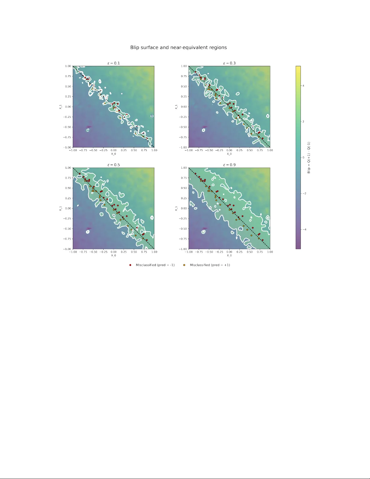
N E A R - E Q U I V A L E N T Q - L E A R N I N G P O L I C I E S F O R D Y N A M I C T R E A T M E N T R E G I M E S Sophia Y azzourh Department of Epidemiology and Biostatistics McGill Univ ersity Montréal, Québec, Canada sophia.yazzourh@mcgill.ca Erica E.M. Moodie Department of Epidemiology and Biostatistics McGill Univ ersity Montréal, Québec, Canada March 23, 2026 A B S T R A C T Precision medicine aims to tailor therapeutic decisions to the indi vidual characteristics of each patient. This objectiv e is commonly formalized through the framework of dynamic treatment re gimes, which use statistical and machine learning methods to deriv e sequential decision rules adapted to ev olving clinical information. In most existing formulations, these approaches produce a single optimal treatment recommendation at each stage, leading to a unique sequence of decision rules. Howe ver , in many clinical settings se veral treatment options may yield very similar expected outcomes, and restricting attention to a single optimal policy may conceal meaningful alternati ves. In this work, we extend the Q-learning framework for retrospective data to incorporate a worst-v alue tolerance criterion controlled by a tuning hyperparameter ε , which specifies how far a polic y is allowed to de viate from the optimal expected v alue. Rather than identifying a single optimal policy , the proposed approach constructs sets of ε -optimal policies whose expected value remains within a controlled neighborhood of the optimum. Conceptually , this formulation shifts the Q-learning problem from a vector-v alued representation, in which a single v alue function determines the optimal decision, to a matrix-valued representation where multiple admissible value functions coe xist during the backw ard recursion. This leads to families of near -equiv alent treatment strategies instead of a single deterministic rule and explicitly characterizes regions of treatment indif ference where sev eral decisions achieve comparable expected outcomes. The proposed frame work is illustrated through two settings. First, in a single- stage treatment decision problem, we e xamine ho w the admissibility criterion induces re gions of treatment indifference around the decision boundary . Second, in a multi-stage treatment decision process, we apply the method within a sequential decision frame work based on a simulated oncology model describing the joint ev olution of tumor size and treatment toxicity . K eywords Precision Medicine · Dynamic T reatment Regimes · Q-learning · Reinforcement Learning 1 Introduction Precision medicine (Kosorok and Laber, 2019) places individual patient characteristics at the center of treatment decisions, with the goal of matching each patient with the treatment e xpected to confer the greatest clinical benefit. This question is particularly relev ant in longitudinal settings with multiple decision points, as commonly encountered in the management of chronic diseases such as cancer, diabetes, or mental health disorders. Dynamic Treatment Re gimes (DTRs) (Chakraborty and Moodie, 2013; K osorok and Moodie, 2015) provide a formal frame work for this paradigm by defining sequences of decision rules that adapt treatment recommendations to e volving patient characteristics. Over the last two decades, numerous methods hav e been proposed to estimate optimal DTRs, which can broadly be di vided into two families. On the one hand, nonparametric methods such as in verse probability of treatment weighting (Robins, 2000), marginal structural models (Robins, 2000; Orellana et al., 2010), and outcome weighted learning (Zhao et al., 2012) aim to directly learn optimal strategies without imposing strong parametric assumption. On the other hand, regression-based approaches including G-estimation (Robins, 1992, 1989, 1998), dynamic weighted ordinary least A P R E P R I N T - M A R C H 2 3 , 2 0 2 6 squares (W allace and Moodie, 2015), and Q-learning (Clifton and Laber, 2020) rely on statistical modeling to estimate how different treatment decisions w ould affect patient outcomes, thereby identifying strategies that maximize clinical benefits. In this paper , we focus on Q-learning, a method rooted in reinforcement learning that frames treatment selection as a sequence of decision problems. At each stage, the method e valuates the e xpected benefit of each possible treatment, taking into account both immediate outcomes and their potential influence on future stages of care. By w orking backward from the final stage, these ev aluations are combined to deri ve strategies that guide treatment choices in a way that maximizes overall patient benefit. Q-learning relies on re gression models to estimate stage-specific v alue functions, which makes it particularly appealing in clinical applications. P arametric and semi-parametric modeling approaches are often familiar to practitioners, allo w straightforward model selection and interpretation, and can be implemented using standard statistical tools while remaining flexible enough to capture comple x treatment–cov ariate interactions. For these reasons, Q-learning has been widely adopted in precision medicine research and applied across di verse clinical contexts, as documented in revie w articles (Clifton and Laber, 2020; Y azzourh et al., 2025). Despite these advances, most existing methods are designed to identify a single optimal treatment policy . This "one-size-fits-all optimum" may be limiting in practice: clinical decisions often in volv e near-equi v alent strategies, where multiple courses of action yield comparable expected outcomes. Restricting recommendations to a unique policy risks o verlooking clinically acceptable alternati ves, thereby reducing fle xibility and clinician autonomy in the decision-making process. The integration of clinical expertise and domain kno wledge into reinforcement learning algorithms has been increasingly recognized as an important direction for the application of dynamic treatment regimes in healthcare, both to impro ve the realism of treatment recommendations and to foster trust in data-driv en decision tools (Holzinger, 2016; Maadi et al., 2021; Lov e et al., 2023; Holzinger et al., 2019; Y azzourh et al., 2025). Motiv ated by this perspectiv e, we adapt Q-learning to identify sets of near-equi valent treatment policies by retaining treatment decisions whose expected v alue remains within an ε -threshold of the optimal polic y . While multiple-polic y approaches ha ve been explored in online reinforcement learning settings (F ard and Pineau, 2011; T ang et al., 2020), their reliance on direct interaction with the en vironment limits applicability in healthcare contexts where learning must typically rely on pre viously collected clinical data. A related multi-objecti ve frame work incorporating patient preferences has been proposed for of fline settings (Lizotte and Laber, 2016). In contrast, our approach is designed for retrospective clinical datasets under a single-objectiv e paradigm, mapping out therapeutically equi valent treatment pathways while maintaining a primary focus on outcome optimization. In this work, we modify the Q-learning framew ork to allow a controlled le vel of de viation from the estimated optimal value. This makes it possible to identify se veral treatment actions that achie ve similar performance. Our method introduces an ε -selection step during the backward recursion, which allo ws the retention of all treatment decisions whose estimated v alue remains within an ε -neighborhood of the optimum. Conceptually , this modification transforms the classical vector -based formulation of Q-learning into a matrix-based representation in which multiple admissible value functions are propagated through the recursion, ultimately producing sets of near -equiv alent policies rather than a single deterministic rule. The remainder of the paper is organized as follows. Section 2 briefly revie ws the classical Q-learning frame work. Section 3 introduces the proposed near-equiv alent Q-learning approach and describes the ε -selection procedure. Section 4 illustrates the method in a single-stage setting by examining indi vidualized treatment rules and the resulting decision boundaries. Section 5 considers a multi-stage dynamic treatment re gime in a simulated oncology setting. Section 6 concludes with a discussion of the methodological implications and potential extensions. 2 Q-learning Longitudinal clinical data consist of measurements collected sequentially throughout the course of treatment. At baseline, they capture patient cov ariates such as demographic and clinical characteristics (e.g., age, sex, comorbidities, or genetic markers). As treatment progresses, some v ariables are reassessed at follo w-up visits and may e volv e ov er time, reflecting both the patient’ s response to therapy and the natural progression of the disease. At each stage, outcomes are recorded to quantify the benefit of the treatment recei ved up to that point. T ogether , these data describe a dynamic trajectory in which the patient’ s state ev olves in response to past decisions and, in turn, shapes future treatment choices. In the context of precision medicine, a Dynamic T reatment Regime provides a formal framew ork for individualizing care ov er time. W e consider a setting with a finite number of decision stages, indexed by t = 0 , . . . , T , where treatment choices are made at discrete points during the course of care. A DTR is defined as a sequence of decision rules, each specifying ho w treatment should be adapted at a gi ven stage according to the patient’ s history up to that point. Formally , 2 A P R E P R I N T - M A R C H 2 3 , 2 0 2 6 let H t denote the history space av ailable prior to stage t , and let H t ∈ H t denote the corresponding random history . Similarly , let A t denote the treatment space at stage t , and A t ∈ A t the assigned treatment. The outcome subsequently observed is denoted by Y t . The collection π = { π 0 , . . . , π T } defines a DTR, where each decision rule is a mapping π t : H t → A t . For a realized history h t ∈ H t , the rule assigns the treatment a t = π t ( h t ) . Sev eral methodological framew orks hav e been dev eloped to estimate optimal DTRs, and these can broadly be divided into two families. The first family focuses on directly optimizing the value of a re gime, defined as the expected cumulativ e outcome under a gi ven sequence of decisions; the idea is to e valuate ho w well a candidate strate gy would perform in the population without explicitly modeling the outcome process at each stage. Within this frame work, in verse probability weighting and marginal structural models (Robins, 2000; Orellana et al., 2010) use weighting schemes to correct for time-dependent confounding, while outcome weighted learning (Zhao et al., 2012) formulates the problem as a weighted classification task. Extensions of this approach include backw ard outcome weighted learning (Zhao et al., 2015), which adapts the method to multi-stage settings through backward recursion, and residual weighted learning (Zhou et al., 2017), which replaces ra w outcomes by residuals to improv e stability and reduce v ariance. Despite their differences, these approaches share the common feature of tar geting the regime value directly rather than modeling outcomes sequentially . The second f amily is based on regression formulations, where sequential models are fit to capture the relationship between patient histories, treatment assignments, and outcomes. G-estimation (Robins, 1992, 1989, 1998), dynamic weighted least squares, (W allace and Moodie, 2015), and Q-learning (Clifton and Laber, 2020) all focus on recov ering optimal strategies through sequential regression modeling of outcomes parameterized as structural nested mean models. In each approach, the analytic problem is concei ved as a sequence of regression tasks solv ed backward in time, where each step predicts the cumulativ e outcome under alternati ve treatment choices. These methods deri ve optimal decision rules from recursiv ely specified outcome models. W ithin this regression-based family , Q-learning occupies a central place and will be the focus of what follo ws. Be yond its popularity in applied work, it is conceptually appealing because it mak es explicit the connection between sequential decision problems in medicine and reinforcement learning (Clifton and Laber, 2020; Y azzourh et al., 2025). Originally dev eloped in the context of interacti ve online data, Q-learning was designed to learn strategies by both exploiting accumulated knowledge and exploring ne w actions to improve performance (W atkins, 1989; W atkins and Dayan, 1992). At the heart of this frame work is the notion of a re ward, denoted by R or Y , which provides a quantitative measure of the consequences of each decision; in medical applications, this notion coincides with the observ ed outcome. In Q-learning, the central objects are the Q -functions, which quantify the expected cumulati ve reward (i.e outcome) associated with taking a gi ven action in a gi ven state under a regime π . Intuitiv ely , they measure ho w beneficial it is for a patient i with history h i,t to choose treatment a i,t at time t , while following strategy π thereafter . For patient i ∈ { 1 , . . . , N } , the stage- t Q -function is defined as Q π i,t ( h i,t , a i,t ) = E π " T X t =0 Y i,t ( h i,t , a i,t )      H i,t = h i,t , A i,t = a i,t # . In the context of DTR, the data used for estimation consist of observ ations that hav e already been collected in clinical settings, either through formal clinical trial protocols or through medical decisions made in practice. In reinforcement learning, such datasets are considered offline , and the associated Q -functions are estimated retrospecti vely from pre- existing observ ations.As described in Algorithm 2, the procedure begins by estimating the Q -function at the final stage T and then proceeds backward in time to earlier stages. This approach is commonly referred to as of fline or backward Q-learning. In practice, the true Q -functions are unkno wn and must be estimated from the data. Let ˆ Q t denote the estimator of Q t , obtained by fitting a re gression model that predicts future outcomes from patient histories and treatments. Such estimators may rely on parametric models (e.g., linear or generalized linear models) or on more flexible machine learning methods, including support vector machines or deep neural networks. At the final stage T , the Q -function is estimated by regressing the final outcome on the co variates and treatment. For earlier stages t < T , the regression target is no longer the observed outcome alone but a modified outcome that incorporates the v alue of the best possible future decision. This captures ho w treatment choices at time t influence downstream re wards and links the decision process across time. At each stage, an optimal treatment is obtained by selecting the action associated with the largest estimated Q -value, where a Q -value represents the e xpected cumulativ e outcome for a gi ven patient history h t and treatment choice a at stage t , assuming optimal decisions are followed thereafter . In practice, these Q -v alues are computed by ev aluating the estimated Q function at the specific history and treatment pair ( h t , a ) . 3 A P R E P R I N T - M A R C H 2 3 , 2 0 2 6 This construction is closely related to the potential outcomes framework where Y denotes the observed outcome under the treatment actually recei ved, whereas Y ∗ ( a ) represents the counterfactual outcome that w ould have been observed under an alternativ e treatment a . In the recursi ve estimation procedure, the observed outcome at stage t is replaced by a pseudo-outcome constructed from the estimated model at stage t + 1 , representing the optimal expected future v alues. Using this learned model, we e valuate all feasible future actions (i.e., all counterfactual treatment choices) and retain the one producing the highest value. For the entire sample of N patients, we write the modified outcome in vector form as ˜ y t =      ˜ Y 1 ,t ˜ Y 2 ,t . . . ˜ Y N ,t      =      Y 1 ,t + max a t +1 ˆ Q t +1 ( H 1 ,t +1 , a t +1 ) Y 2 ,t + max a t +1 ˆ Q t +1 ( H 2 ,t +1 , a t +1 ) . . . Y N ,t + max a t +1 ˆ Q t +1 ( H N ,t +1 , a t +1 )      . This representation highlights that for each patient, the unobserved continuation of their trajectory is replaced by the value the y would have obtained under the optimal decision at the next stage. By propagating these optimal counterfactuals backward through time, Q-learning incorporates long-term and delayed treatment effects into the estimation. Once all the Q -functions hav e been estimated across stages, the optimal strategy is obtained by selecting, at each stage t , the action that maximizes the corresponding estimated Q -function: ˆ π ⋆ t ( h t ) = arg max a t ∈A t ˆ Q t ( h t , a t ) . Algorithm 1.Backward Q-learning Input 1: Offline training data consisting of admissible histories H t , treatments A t , and outcomes Y t for t = 0 , . . . , T , and a fitting algorithm (parametric or non-parametric). Final stage T 2: Estimate Q T from ( Y T , H T , A T ) such that ˆ Q T ( h T , a T ) ≜ ˆ E ( Y T | H T = h T , A T = a T ) . 3: for t = T − 1 , . . . , 0 do 4: Compute the pseudo-outcome ˜ Y t = Y t + max a t +1 ˆ Q t +1 ( H t +1 , a t +1 ) . 5: Estimate ˆ Q t ( h t , a t ) ≜ ˆ E  ˜ Y t | H t = h t , A t = a t  . 6: end for Output 7: The estimated optimal policies { ˆ π ⋆ 0 , . . . , ˆ π ⋆ T } with ˆ π ⋆ t ( h t ) = arg max a t ∈A t ˆ Q t ( h t , a t ) . 3 Near -equivalent Q-learning In its standard formulation, Q-learning recommends a single action at each decision point, namely the one that maximizes the estimated expected outcome at time t . While this yields a clear decision rule, it may conceal alternati ve actions, or ev en entire treatment sequences, that achiev e comparable expected outcomes. This limitation is particularly salient in clinical applications. Treatment policies are typically learned from observational or trial data generated under pre-e xisting medical strategies, often shaped by physician judgment or fixed study protocols. Consequently , the estimated policy reflects not only the outcome process b ut also the historical allocation mechanism embedded in the data. The resulting recommendation therefore inherits the exploration–e xploitation structure of the data-generating process. 4 A P R E P R I N T - M A R C H 2 3 , 2 0 2 6 Restricting the analysis to a unique optimal strategy may thus reduce flexibility and obscure near -equiv alent treatment pathways that would be clinically acceptable. When estimated value differences are small, the distinction between optimal and suboptimal actions may be dri ven more by statistical variability than by meaningful clinical contrast. Identifying strategies with comparable expected performance may therefore pro vide a more informative and practically relev ant characterization of the decision landscape. One possible way to address the limitations of single-polic y Q-learning is to construct a frame work that recommends near-equivalent actions , thereby allowing the integration of additional considerations such as treatment in vasi veness, local av ailability , or potential side ef fects. Rather than enforcing strict optimality , such an approach seeks to identify actions whose expected performance remains within a controlled mar gin of the optimal value. From a decision-process perspectiv e, this idea is closely related to the concept of near-optimal policies introduced by Fard and Pineau 2011. In that work, admissible actions are defined through a worst-case value criterion, corresponding to the smallest Q -value retained within the acceptable set. This quantity determines both the permissible deviation from the optimal decision and the minimal performance lev el tolerated among admissible actions. The resulting frame work yields a set of policies whose performance is guaranteed to remain within a predefined threshold. Howe ver , the approach of Fard and Pineau 2011 was de veloped in a fully model-based setting, assuming known transition probabilities, and within an interactive (on-polic y) en vironment where the policy is optimized through direct interaction with the system. These assumptions differ substantially from real-w orld Dynamic T reatment Regime applications, which rely on observational or trial data and do not permit interacti ve policy refinement. The method was subsequently extended by T ang et al. 2020 to a model-free context and an of f-policy setting, where the en vironment is first explored and then e xploited in a separate optimization phase. Although this extension relax es the requirement of known transition dynamics, it remains situated within an online learning paradigm and was e valuated in a simulated intensi ve-care frame work based on MIMIC data. As such, it does not align with the constraints of of fline DTR estimation. Finally , the notion of multiple admissible policies has also been e xplored in a multi-objecti ve reinforcement learning frame work by Lizotte and Laber 2016. In that setting, the reward is vector-v alued and reflects several competing clinical objecti ves. The authors introduce a dominance concept of P areto dominance, incorporating patient preferences. Applied to the CA TIE study , this approach enables the identification of treatment strategies that balance multiple outcomes while remaining clinically interpretable. While conceptually related, existing approaches typically operate in model-based, interactive, or multi-objecti ve settings. In contrast, our objective is to introduce controlled near -optimal admissibility within a single-objectiv e, offline, regression-based Dynamic Treatment Regime framew ork. T o this end, we consider a finite-horizon DTR setting in which Q -functions are estimated via classical backw ard Q-learning. Let T denote the terminal stage. As described pre viously , standard backw ard Q-learning proceeds recursiv ely from stage T to stage 0 , assuming that the optimal action is taken at subsequent stages when constructing pseudo-outcomes. Our goal is to embed near -optimal admissibility within this regression-based recursion while preserving its structural inte grity . The admissibility criterion introduced by F ard and Pineau 2011 is originally formulated in terms of value functions, which are assumed to be positiv e. In their framework, a subset of actions S ⊆ A t is considered ε -admissible if min a ∈ S V ( h t , a ) ≥ (1 − ε ) max a ∈A t V ( h t , a ) . This definition relies on a worst-case perspecti ve: the minimum v alue within the admissible set must remain within a (1 − ε ) margin of the optimal (i.e., maximal) v alue, ensuring that e ven the least f av orable admissible action remains close to the optimum. Applying this condition directly within a Q-learning framework w ould require imposing the same criterion on the estimated Q-functions. Ho wev er , unlike the value functions considered in the original formulation, Q-functions are not necessarily positi ve. Consequently , the multiplicati ve formulation abo ve may lead to undesirable beha vior when max a ∈A t ˆ Q t ( h t , a ) is neg ativ e. T o address this issue, we adopt the follo wing admissibility condition. For a giv en history h t , an action a ∈ A t is considered admissible if ˆ Q t ( h t , a ) ≥ max a ∈A t ˆ Q t ( h t , a ) − ε     max a ∈A t ˆ Q t ( h t , a )     . This condition ensures that the estimated v alue of an y retained action lies within an ε -neighborhood of the optimal esti- mated value. Equi valently , the maximal tolerated loss relative to the optimal action is bounded by ε    max a ∈A t ˆ Q t ( h t , a )    . The hyperparameter ε therefore controls the tolerated deviation from optimality . When ε = 0 , the procedure reduces to classical Q-learning, whereas increasing values of ε progressiv ely enlarge the set of near -optimal admissible actions. 5 A P R E P R I N T - M A R C H 2 3 , 2 0 2 6 The role of ε can be further clarified by examining its boundary cases. When ε = 0 , the admissibility condition reduces to ˆ Q t ( h t , a ) ≥ max a ∈A t ˆ Q t ( h t , a ) , which implies that only actions whose estimated value is strictly equal to the maximal estimated v alue are retained. At the other extreme, when ε = 1 , the condition becomes ˆ Q t ( h t , a ) ≥ max a ∈A t ˆ Q t ( h t , a ) −     max a ∈A t ˆ Q t ( h t , a )     . T wo situations may arise. If the estimated Q-functions are strictly positi ve, the condition reduces to ˆ Q t ( h t , a ) ≥ 0 . One might therefore expect that all strate gies would be retained when re wards are strictly positi ve. Howe ver , in practice, Q-functions are estimated through regression models that do not constrain predictions to remain within the range of the observed outcomes. Many regression procedures allow extrapolation beyond the support of the tar get variable. For example, in the second implementation presented in Section 5, we use a support vector re gression model with a radial basis function (Gaussian) kernel, which does not enforce positivity of predictions e ven when all observed re wards are positive. More generally , unless explicit constraints are imposed, estimated Q-values may take negati ve values. Consequently , ε = 1 does not guarantee that all strategies are retained, and the admissibility criterion becomes ill-posed at that boundary . If the maximal estimated Q-value is neg ativ e, the condition also becomes difficult to interpret, since the admissibility threshold may no longer correspond to a clear notion of near-optimality . For these reasons, we restrict the hyperparameter to ε ∈ [0 , 1[ to ensure a well-defined and controlled relaxation of optimality . The hyperparameter ε therefore controls the maximal loss tolerated with respect to the optimal treatment. Importantly , this loss is defined relative to the magnitude of the maximal estimated value. In other words, the admissibility threshold is not defined by a fixed distance from the optimum, b ut by a proportion of the size of the best estimated effect. When max a ∈A t ˆ Q t ( h t , a ) is large, the admissible band becomes wider, reflecting the fact that sev eral actions may yield similar large e xpected benefits. Con versely , when the maximal estimated value is small, the admissible band becomes narrower , meaning that only actions very close to the optimum are retained. Under this admissibility criterion, the decision rule at stage t becomes set-v alued rather than single-valued, mapping each history h t to a subset of A t containing all actions whose estimated value lies within the prescribed tolerance of the optimum. The sequential composition of these admissible sets across stages therefore defines a collection of near-equi valent treatment trajectories instead of a unique strate gy . A necessary condition for implementation is that the action space A t be finite and discrete, allo wing explicit comparison across actions; in DTR applications, this assumption is natural, as treatment regimens are clinically predefined and finite. A direct application of ε -selection at e very stage would disrupt the recursi ve structure of backw ard Q-learning. Standard recursion relies on the assumption that a unique optimal action is taken at future stages when constructing pseudo- outcomes. Allo wing set-valued actions at all stages w ould therefore break this dependency structure and lead to a combinatorial expansion of candidate trajectories. Thus, to preserve the classical backward scheme, we introduce ε -selection only at the penultimate stage. Applying the selection at stage T − 1 allows identification of near -equiv alent treatment trajectories while preserving a unique optimal action at the terminal stage. If selection were introduced at the terminal stage alone, potentially suboptimal de viations could propagate backw ard and accumulate error . By contrast, selecting at the second-to-last stage captures multiple clinically comparable strategies while maintaining consistenc y with the estimated optimal outcome at T . At stage T , a single ˆ Q T is estimated. When ε -selection is applied at stage T − 1 , for each patient i , it yields a set of n i admissible Q -functions, denoted Q 1 i,T , . . . , Q n i i,T . Let m = max i ∈{ 0 ,...,N } ( n i ) , m ≤ |A T | . Since regression at stage T − 2 relies on pseudo-outcomes derived from stage T − 1 , these quantities must share a common dimension across indi viduals in order to fit a single regression model and maintain a coherent recursi ve structure. Let m denote the maximum number of admissible actions observed at stage T − 1 . F or each individual, we therefore construct a pseudo-outcome v ector of length m . When n i < m , the vector is completed by padding with repeated ev aluations of the first optimal Q -function until dimension m is reached. This construction yields a square and uniformly dimensioned pseudo-outcome matrix at stage T − 2 , simplifying the backward recursion at earlier stages and av oiding stage-specific model specifications. Importantly , the padding operation neither alters the relative ordering of 6 A P R E P R I N T - M A R C H 2 3 , 2 0 2 6 admissible actions nor changes the long-term optimization objectiv e; it preserves the v alue structure induced by the estimated Q -functions while ensuring the dimensional alignment required for stable and consistent recursiv e estimation. Consequently , for stages t < T − 1 , the pseudo-outcome no longer takes the form of a vector as in Section 2, but becomes a matrix ˜ Y t of dimension ( N × m ) , where m denotes the maximum number of per -individual Q -functions retained under the ε -selection criterion at stage T . Specifically , ˜ Y t =    ˜ Y 1 1 ,t . . . ˜ Y m 1 ,t . . . . . . . . . ˜ Y 1 N ,t . . . ˜ Y m N ,t    , where, for j ∈ { 1 , . . . , m } , ˜ Y j i,t ( h i,t ) = Y i,t ( h i,t ) + max a ˆ Q j i,t +1 ( h i,t +1 , a ) . For each j , a separate regression model is fitted using the pseudo-outcome vector ˜ y j t (the j -th column of ˜ Y t ), yielding the corresponding estimator ˆ Q j t . The backward recursion therefore proceeds as in classical Q-learning, except that it is carried out in parallel across the m retained models. The complete procedure is summarized in Algorithm ?? and produces a collection of ε -equiv alent treatment strategies within a standard regression-based DTR frame work. Rather than discarding optimality , the method relaxes it in a controlled manner go verned by the hyperparameter ε , thereby preserving the long-term optimization objectiv e while allowing multiple near -optimal treatment trajectories. Clinically , this approach enables identification of patients located near decision boundaries, for whom multiple actions yield similar expected outcomes. For such patients, e xternal considerations such as toxicity , a vailability , cost, or patient preference may legitimately guide the final choice without materially compromising expected performance. Methodologically , the approach remains fully grounded in backward Q-learning, requiring only a modified pseudo- outcome construction at stage T − 1 . In the follo wing section, we e valuate the proposed method in tw o complementary settings. W e first consider a simulated Individualized T reatment Regime scenario (i.e., a single-stage decision process setting) with binary treatment, which allows for a clear in vestigation of the role of the hyperparameter ε and highlights the ability of the method to detect patients located near the decision boundary . W e then illustrate the approach in a multi-stage DTR setting with six treatment stages in a simulated oncology framework to assess its practical performance and potential clinical rele vance. All code and simulation results are publicly av ailable on a dedicated GitHub repository 1 . Algorithm 2. Near -Equivalent Q-learning Input : Of fline training data consisting of i ∈ { 1 , . . . , N } patients, each with admissible histories h i,t and associated re wards Y i,t for t ∈ { 0 , . . . , T } . The algorithm also requires a fitting method (parametric or non-parametric) and a hyperparameter ε ∈ [0; 1[ that specifies the allowed de viation from the optimal polic y . Final stage T : Estimation: Estimate Q T based on Y T ∼ H T , A T , such that ˆ Q T ( h T , a T ) ≜ ˆ E ( Y T | H T = h T , A T = a T ) . At this stage, we obtain a single estimated Q -function, denoted ˆ Q T . Penultimate stage T − 1 : 1. ε -Selection : for each patient i , identify the subset of estimated Q T -functions whose v alue satisfies the ε -admissibility condition, ˆ Q i,T ( h i,T , a ) ≥ max a ∈A T ˆ Q i,T ( h i,T , a ) − ε     max a ∈A T ˆ Q i,T ( h i,T , a )     . Let n i denote the number of estimated Q -functions satisfying this criterion for patient i . W e then construct the vector h ˆ Q 1 i,T , . . . , ˆ Q n i i,T i , containing the admissible estimated Q -values for patient i . 2. Padding : Let m = max i ∈{ 1 ,...,N } ( n i ) denote the maximum number of per -individual Q -functions satisfying the ε -selection criterion at stage T , where m ≤ |A T | and |A T | denotes the cardinality of 1 https://github.com/sophiayazzourh/Multiple_Policies_Qlearning 7 A P R E P R I N T - M A R C H 2 3 , 2 0 2 6 the action space. W e construct an ( N × m ) matrix in which the i -th ro w consists of the n i selected elements [ ˆ Q 1 i,T , . . . , ˆ Q n i i,T ] , followed, when n i < m , by ( m − n i ) copies of ˆ Q 1 i,T to ensure common dimensionality across patients. This results, for each patient i , in a v ector of dimension (1 × m ) giv en by h ˆ Q 1 i,T , . . . , ˆ Q m i,T i . 3. Pseudo-outcome matrix: construct the pseudo-outcome matrix ˜ Y T − 1 of dimension ( N × m ) : ˜ Y T − 1 =    ˜ Y 1 1 ,T − 1 . . . ˜ Y m 1 ,T − 1 . . . . . . . . . ˜ Y 1 N ,T − 1 . . . ˜ Y m N ,T − 1    , where, for j ∈ { 1 , . . . , m } , ˜ Y j i,T − 1 ( h i,T − 1 ) = Y i,T − 1 ( h i,T − 1 ) + max a ˆ Q j i,T ( h i,T , a ) . 4. Estimation : Estimate the functions Q j T − 1 by fitting separate regressi ons to each column of ˜ Y T − 1 . Let ˜ y j T − 1 denote the pseudo-outcome vector associated with model j , i.e., the j -th column of ˜ Y T − 1 . For j = 1 , . . . , m , we define ˆ Q j T − 1 ( h T − 1 , a T − 1 ) ≜ ˆ E  ˜ y j T − 1 | H T − 1 = h T − 1 , A T − 1 = a T − 1  . At stage T − 1 , this yields a collection of m optimal and near-optimal Q -functions: n ˆ Q 1 T − 1 , . . . , ˆ Q m T − 1 o . Stages t < T − 1 : 1. Pseudo-outcome matrix: construct the pseudo-outcome matrix ˜ Y t of dimension ( N × m ) : ˜ Y t =    ˜ Y 1 1 ,t . . . ˜ Y m 1 ,t . . . . . . . . . ˜ Y 1 N ,t . . . ˜ Y m N ,t    , where, for j = 1 , . . . , m , ˜ Y j i,t ( h i,t ) = Y i,t ( h i,t ) + max a ˆ Q j i,t +1 ( h i,t +1 , a ) . 2. Estimation : For j = 1 , . . . , m , estimate the functions Q j t by fitting separate regressions to each column of ˜ Y t . Let ˜ y j t denote the pseudo-outcome v ector associated with model j , i.e., the j -th column of ˜ Y t . W e define ˆ Q j t ( h t , a t ) ≜ ˆ E  ˜ y j t | H t = h t , A t = a t  . At each stage t , this yields a collection of m optimal and near-optimal Q -functions: n ˆ Q 1 t , . . . , ˆ Q m t o . Construction of ε -equivalent estimated policy sets ˆ Π T : At each stage t , we construct a set of near -equiv alent actions. The sequential combination of these actions defines a set of near-equi valent strategies such that, for j ∈ { 1 , . . . , m } , ˆ Π j ( h ) = h ˆ π j 0 ( h 0 ) , . . . , ˆ π j T ( h T ) i , where ˆ π j t ( h t ) = arg max a t ∈A t ˆ Q j t ( h t , a t ) . 8 A P R E P R I N T - M A R C H 2 3 , 2 0 2 6 4 Individualized T reatment Regimes: decision boundaries and the role of ε W e consider a single-stage individualized treatment regime and simulate data according to (Song et al., 2015). F or each simulated patient, covariates X 0 , . . . , X 9 are generated independently and identically distrib uted as U ([ − 1 , 1]) , and A ∈ {− 1 , 1 } with P ( A = 1) = 1 / 2 . The outcome is generated as Y ∼ N  1 + 2 X 0 + X 1 + 0 . 5 X 2 + T 0 ( A, X ) , 1  , where T 0 ( A, X ) = ( X 0 + X 1 ) A . The true indi vidualized treatment ef fect is τ ( X ) = X 0 + X 1 , the optimal rule is π ⋆ ( X ) = sign( X 0 + X 1 ) , and the true decision boundary is the linear surface X 0 + X 1 = 0 . W e implement a one-stage Q-learning procedure using a linear working model for the Q -function. Specifically , we estimate b Q ( X, A ) = b β 0 + b β ⊤ X X + b β A A + b β ⊤ AX ( AX ) , where treatment–cov ariate interaction terms allo w for heterogeneous treatment effects. The model is fitted on the training sample using a linear re gression with regressors [1 , X 0 , . . . , X 9 , A, AX 0 , . . . , AX 9 ] , i.e., including all co variates and all treatment–cov ariate interaction terms. For each subject in the test set, predicted values are computed under both treatment options A = − 1 and A = +1 , yielding the estimated v alue pair  b Q ( X, − 1) , b Q ( X, +1)  . In the one-stage binary-treatment setting, the role of ε is naturally understood through the blip function, defined as the difference between the Q -values e valuated under each of the two treatment options, ∆( X ) = Q ( X , 1) − Q ( X , − 1) . The blip fully determines the indi vidualized treatment rule: its sign specifies the optimal action, while its magnitude reflects the strength of the treatment preference. From a reinforcement learning perspecti ve, ∆( X ) corresponds to a relativ e advantage function, quantifying ho w much better one action performs compared to the alternativ e at the same cov ariate profile. In this setting, ε -selection is constructed directly from the estimated blip b ∆( X ) = b Q ( X, 1) − b Q ( X, − 1) by retaining both treatments whenev er | b ∆( X ) | ≤ ε , equiv alently including all actions whose predicted value lies within ε of the maximal predicted Q -value. Geometrically , this replaces the sharp decision boundary b ∆( X ) = 0 with a band defined by | b ∆( X ) | ≤ ε . As ε increases, this band widens, identifying regions of the cov ariate space where the difference in expected outcomes between treatments is small and where no clearly dominant choice emer ges. Figure 1 displays the estimated blip surface projected onto the ( X 0 , X 1 ) plane. Positi ve regions (yello w) indicate preference for treatment +1 , while negati ve regions (purple) fa vor treatment − 1 . The smooth transition of the surface reflects the linear treatment–cov ariate interaction used in the data-generating mechanism. Misclassified points are primarily located near the true decision boundary , where the treatment effect is close to zero and small estimation fluctuations may alter the sign of the blip. The white band corresponds to the ε -selection region defined by | b ∆( h ) | ≤ ε . This band encompasses most misclassified observations and identifies regions where the expected dif ference between treatments is small. Rather than imposing a sharp boundary , the ε -selection frame work explicitly ackno wledges that, in these areas, no clearly dominant treatment emerges. This perspectiv e is related in spirit to earlier approaches that address instability near the decision boundary through hard- or soft-thresholding (Moodie and Richardson, 2010; Chakraborty et al., 2010), although the present framework dif fers in that it yields a set of admissible treatments rather than modifying the decision rule itself. In contrast, misclassifications are rare in regions where the blip has large magnitude, indicating that the model reliably identifies the optimal treatment when the signal is strong. Overall, the concentration of apparent errors near the ε -band suggests that they reflect intrinsic ambiguity in treatment preference rather than model inadequac y . 5 Cancer Simulation Study: A Multistage Multiple-T reatment Decision Pr oblem The goal of this section is to illustrate the behavior of the proposed approach in a setting with multiple treatments and multiple stages. As a point of reference, we consider standard Q-learning, since our method is e xplicitly designed as an extension of it, modifying only the decision rule while preserving the underlying estimation procedure. Existing approaches for constructing set–valued or near–optimal treatment rules are typically dev eloped in model-based, interactiv e, or multi–objective settings (Fard and Pineau, 2011; Lizotte and Laber, 2016; T ang et al., 2020), and do not directly accommodate the of fline, regression-based Dynamic T reatment Regime framework considered here. Consequently , there are currently no direct comparable methods that address the same data structure. W e illustrate the proposed method using a simulated dataset based on the model proposed by Zhao et al. (2009), a benchmark frequently used in reinforcement learning studies (Fürnkranz et al., 2012; Akrour et al., 2012; Goldberg and K osorok, 2012; Humphrey, 2017; Y azzourh, 2024). The model represents a simplified form of chemotherapy management in a non-specific cancer population, where treatment decisions are made monthly o ver a six-month period. 9 A P R E P R I N T - M A R C H 2 3 , 2 0 2 6 Figure 1: Estimated blip surface b ∆( X ) = b Q ( X, 1) − b Q ( X, − 1) projected onto the ( X 0 , X 1 ) plane for increasing values of ε . The dashed line represents the true decision boundary X 0 + X 1 = 0 . White contours indicate the ε -selection region defined by | b ∆( X ) | ≤ ε . At each time t = 0 , . . . , 6 , the patient’ s state S t = ( T t , X t ) includes tumor size T t and treatment toxicity X t . The administered dose A t ranges from 0 to 1 in increments of 0 . 1 . T umor and toxicity dynamics are gov erned by coupled differential equations describing tumor reduction due to treatment, drug toxicity accumulation, and remission once T t = 0 . Mortality is modeled by a survi val process with hazard λ ( t ) = exp( − 4 + T t + X t ) , reflecting the combined effect of tumor b urden and toxicity on survi val probability . The reward at each stage t is defined as the sum of three components capturing (i) survi v al status, (ii) change in toxicity , and (iii) tumor response, with R t = R t, 1 + R t, 2 + R t, 3 , where R t, 1 = − 60 if death occurs at stage t and 0 otherwise, R t, 2 = 5 if X t +1 − X t ≤ − 0 . 5 and − 5 otherwise, and R t, 3 = 15 if T t +1 = 0 , 5 if T t +1 − T t ≤ − 0 . 5 and T t +1  = 0 , and − 5 otherwise. Each patient trajectory is thus characterized by sequential trade-offs between ef ficacy and tolerability , providing a suitable en vironment for ev aluating decision rules under multiple near-equi valent treatment sequences. From this simulation model, we generated a training sample of 500 patients under a randomized treatment strategy and fitted our models using both classical backward Q-learning (Algorithm 2) and the proposed Near-Equi valent Q-learning procedure (Algorithm ?? ). In both approaches, the same regression model was employed, namely a support v ector regression with radial basis function kernel (def ault C = 1 . 0 ), ensuring comparability between methods. T o illustrate the behavior of the proposed approach under different le vels of admissibility , we consider sev eral values of the hyperparameter ε ∈ { 0 . 1 , 0 . 3 , 0 . 5 , 0 . 9 } . For each v alue of ε , the ε -selection criterion is applied within the backward recursion to identify sets of near-equi valent policies. 10 A P R E P R I N T - M A R C H 2 3 , 2 0 2 6 The resulting treatment strategies are ev aluated by simulating trajectories on an independent test sample of 5000 patients generated under identical initial conditions. Figure 2 displays, over a six-month horizon, the combined a verage tumor size and toxicity experienced by these patients under the different treatment strate gies. The dashed curves correspond to constant treatment regimes ranging from 0.1 to 1.0, while the red solid line (“opt”) represents the polic y learned via classical Q-learning. The dashed curves correspond to the near -equiv alent policies identified by our method, and the shaded red region illustrates the ε -tolerance band around the optimal trajectory . Each panel corresponds to a different value of the admissibility parameter ε . All learned policies produce consistently lo wer values of the combined tumor size—toxicity metric than the constant treatment regimes across the entire time horizon. Since lo wer v alues correspond to a better trade-of f between tumor burden and treatment toxicity , this indicates that adapti ve treatment strategies achie ve more f av orable overall outcomes than fixed-dose regimes. The first-ranked near -equiv alent policy , in terms of value, perfectly ov erlaps with the classical optimal policy , confirming that the proposed framew ork recovers the standard Q-learning solution when ε is small. As ε increases, the admissible band gradually widens, reflecting a controlled relaxation of optimality . Nev ertheless, the resulting policies remain visually almost indistinguishable from the optimal trajectory and consistently outperform all constant treatment regimes. This indicates that the policy with the highest value within the near-equi valent set remains very similar across v alues of ε . This pattern also suggests that the v alue function exhibits a relati vely flat region around the optimum. In other w ords, se veral treatment strategies produce nearly identical expected outcomes, indicating that the optimal policy is not isolated but lies within a plateau of near -optimal solutions. The proposed framew ork e xplicitly characterizes this re gion by identifying sets of ε -equiv alent policies. Moreover , the performance gap between constant and learned treatment strategies increases o ver time, reflecting the cumulati ve impact of sequential decision-making and illustrating the stability of the backward learning process under a controlled relaxation of optimality . Moreov er , the performance gap between constant and learned treatment strate gies increases ov er time, reflecting the cumulativ e nature of sequential decision-making and illustrating the stability of the backw ard learning process under a controlled relaxation of optimality . W e also report the computational cost of the proposed procedure. All computations were performed in Python on a laptop equipped with an Apple M1 processor (16 GB RAM). T raining the classical Q-learning model required approximately 0 . 29 seconds, whereas training the near-equi valent Q-learning procedure required about 2 . 1 seconds for a giv en value of ε . Although the simulation model captures ke y aspects of dynamic treatment decisions, it remains a simplified repre- sentation of the clinical process and is primarily designed to illustrate the methodological behavior of the proposed approach. The limitations of this simulation design and their implications for practical applications are discussed in the next section. 6 Discussion This work introduces a framew ork for identifying near-equi valent treatment policies within the Q-learning paradigm . While classical Q-learning focuses on estimating a single optimal policy , the proposed approach relax es this objectiv e by identifying sets of policies whose expected value remains within a controlled tolerance of the optimum. Rather than producing a single deterministic rule, the method characterizes f amilies of treatment strategies that are nearly optimal according to a user -defined admissibility h yperparameter ε . This formulation reflects the practical reality that, in many clinical settings, se veral treatment options may lead to v ery similar expected outcomes. Consequently , restricting attention to a single optimal polic y may obscure meaningful alternati ves and gi ve the impression of a sharply defined decision boundary where little dif ference in expected benefit actually e xists. By explicitly identifying sets of near-optimal strate gies, the proposed framework pro vides a richer representation of treatment decisions and highlights situations in which the optimal choice is inherently unstable. The hyperparameter ε controls the tolerance for near -optimality in the treatment recommendation. Conceptually , ε represents the maximum acceptable loss in expected outcome relativ e to the optimal treatment. In this work, ε is interpreted as a tolerance on the dif ference in expected outcome between competing treatment options, allo wing for flexible treatment recommendations in re gions where these differences are small. In applications to clinical data, several practical strategies could guide the choice of ε . When the outcome scale is arbitrary or model-dependent, it may be con venient to define ε relativ e to the empirical distrib ution of the estimated blip function. For instance, ε could be selected as a fixed fraction of the standard deviation of the blip or as a low quantile of | ∆( h ) | . Such scale-relativ e choices may provide a pragmatic way to calibrate the tolerance lev el when no natural clinical scale is a vailable. Another possible interpretation is to vie w ε as a mechanism for controlling the size of the near -indifference re gion. By selecting ε so that a predetermined proportion of indi viduals satisfies | ∆( h ) | ≤ ε , 11 A P R E P R I N T - M A R C H 2 3 , 2 0 2 6 Figure 2: Combined average tumor size and toxicity o ver six stages for 5000 simulated patients under identical initial conditions ( n train = 500 , n test = 5000 ). Each panel corresponds to a different v alue of ε , illustrating how the admissible set of policies expands as the tolerance increases. Dashed lines correspond to constant treatment regimes ranging from 0.1 to 1.0. The red solid line (“opt”) represents the policy learned via classical backward Q-learning. Bold dashed lines denote the ε -equiv alent policies obtained with the proposed method. The shaded red band indicates the ε -tolerance region around the optimal polic y . one could regulate the fraction of the population for which the treatment recommendation becomes set-v alued rather than deterministic. From this perspecti ve, ε acts as a policy-le vel tuning parameter gov erning the trade-off between decisiv eness and flexibility . More generally , the choice of ε would ideally incorporate clinical considerations, since the acceptable de viation from optimality depends on the practical consequences of treatment dif ferences. Future work could therefore explore approaches that combine empirical calibration with clinically meaningful thresholds when selecting ε . From a statistical standpoint, ε may also be linked to estimation uncertainty . When uncertainty quantification for the blip function is a vailable, for instance through bootstrap or Bayesian procedures, ε may be chosen to reflect the typical magnitude of estimation error . Treatments are then considered near-optimal when differences in estimated Q -values cannot be distinguished giv en the uncertainty of the model. Interpreting ε as a tolerance on instantaneous regret therefore pro vides a unified perspective linking clinical rele vance, statistical uncertainty , and reinforcement learning principles. Sev eral design choices were considered when inte grating the ε -selection step within the backward Q-learning recursion. In the proposed implementation, the selection is performed at the penultimate stage of the algorithm. Introducing the criterion at the final stage w ould effecti vely impose the admissibility condition on a transformed v ersion of the final outcome, which could lead to cumulativ e drift when propagated backward through the re gression steps. Con versely , introducing the ε -selection too early in the recursion would collapse the decision process to a single policy in subsequent stages due to the structure of the backward re gression updates. The penultimate stage therefore represents a natural compromise, allo wing the admissible set of policies to expand while preserving a direct connection with the final objectiv e. W e also considered applying the ε -selection criterion at e very stage of the backward recursion. Such an approach would generate a branching structure of candidate policies whose size grows exponentially with the number of stages and the cardinality of the action space. In addition to the resulting computational b urden, many of the resulting policies would be identical, making the criterion insufficiently restricti ve in practice. 12 A P R E P R I N T - M A R C H 2 3 , 2 0 2 6 From the perspecti ve of individualized treatment rules illustrated in Section 4, the admissibility criterion naturally defines regions of treatment indif ference. When these regions are large, the resulting policy may recommend multiple treatments for a gi ven patient because the estimated treatment effects are very similar . In such situations, enforcing a single treatment recommendation may be arbitrary and ov erly sensitiv e to estimation noise. The proposed framework instead explicitly ackno wledges this ambiguity by identifying sets of ε -optimal treatments. Consequently , se veral treatments may reasonably be considered acceptable, allowing external considerations such as patient preference, treatment accessibility , cost, or safety to inform the final decision. More broadly , the width of the admissible re gion can be interpreted as an indicator of treatment indifference: narro w regions correspond to clear treatment preference, whereas wider re gions indicate that multiple treatments yield nearly identical expected outcomes. In this way , the proposed method pro vides additional insight beyond a single optimal rule by characterizing the stability of the treatment decision. When considered in the context of dynamic treatment re gimes presented in Section 5, the proposed frame work identifies sets of sequential policies whose cumulativ e value remains within an ε -neighborhood of the optimal policy . Rather than focusing exclusi vely on a single optimal sequence of decisions, the method characterizes f amilies of near-optimal strategies that produce similar long-term outcomes. This perspecti ve is particularly relev ant in sequential decision problems where treatment effects accumulate o ver time, as small deviations from the optimal decision at a gi ven stage may have only limited impact on the overall outcome, leading to multiple policies with v ery similar v alue. Identifying such policies therefore pro vides insight into the stability of the sequential decision process and may facilitate the integration of practical constraints or expert judgment into the final treatment strategy . The simulation setting considered in this work is intentionally simplified and does not fully reflect the complexity typically encountered in precision medicine applications. In particular , the state space includes only tw o covariates describing tumor size and toxicity , which limits the heterogeneity of patient profiles and reduces the potential for highly individualized treatment recommendations. Moreover , patient trajectories are generated through a deterministic dynamical system based on ordinary dif ferential equations. Although this formulation captures interactions between tumor progression and treatment toxicity , it also produces relativ ely smooth and structured trajectories, resulting in limited v ariability in the state space and potentially contributing to the relati vely stable set of near-equi valent policies observed in the simulation results. These simplifications were deliberately adopted to provide a controlled en vironment in which the methodological beha vior of the proposed frame work can be clearly illustrated. In more realistic clinical settings in volving higher -dimensional patient histories and more complex stochastic dynamics, the structure of near -equiv alent policies may be substantially richer . The additional computational cost induced by the proposed framework remains moderate and primarily reflects the identification of multiple admissible treatment strategies during the backw ard recursion. In practice, the number of near-equi valent strategies that may be e xplored is naturally bounded by the size of the action space, so the complexity of the procedure remains directly linked to the number of a vailable treatment options. Sev eral extensions of the proposed frame work deserve further inv estigation. First, uncertainty quantification for near-equi valent treatment strate gies could be de veloped using bootstrap procedures applied to the entire learning process. Such an approach would allo w the construction of confidence measures for the admissible treatment sets and provide additional insight into the stability of the recommended strategies. Ho wev er , this task is complicated by the presence of near -equi valent treatment options, which naturally raises questions of non-identifiability , as small differences in estimated value may not be statistically distinguishable. In such regions, the decision rule may exhibit non-smooth behavior , leading to non-standard asymptotics and potentially limiting the v alidity of standard bootstrap procedures. Addressing these challenges may require the dev elopment of alternativ e inferential tools tailored to set-v alued or near-indif ferent decision problems. Second, the current implementation estimates a separate re gression model for each action. An interesting extension would consist in estimating the Q-function through vector-v alued or multi-output re gression models, allowing informa- tion to be shared across treatment options. Related ideas hav e been explored in the context of joint or shared-parameter estimation approaches (W ang et al., 2022), which aim to improve statistical ef ficiency by lev eraging common structure across treatments. Such approaches could potentially enhance estimation when v alue functions associated with dif ferent treatments are similar . In this setting, because only the outcome corresponding to the treatment actually recei ved is observed for each individual, multi-output formulations would require careful modeling to account for this partially observed structure and to a void introducing bias in the estimation of treatment ef fects. Finally , the proposed ε -selection framew ork is not restricted to classical Q-learning and could potentially be combined with other regression-based methods for estimating individualized treatment rules, such as dynamic weighted ordinary least squares or G-estimation. Applying the approach to real-world datasets in volving multiple treatment alternati ves represents an important direction for future work. 13 A P R E P R I N T - M A R C H 2 3 , 2 0 2 6 Acknowledgments Erica E. M. Moodie is a Canada Research Chair (T ier 1) in Statistical Methods for Precision Medicine, funded by the Canadian Institutes of Health Research (CIHR). This work w as supported by a Discovery Grant from the Natural Sciences and Engineering Research Council of Canada (NSERC). Computational resources were provided by the Digital Research Alliance of Canada (Alliance Canada). Financial disclosure None reported. Conflict of interest The authors declare no potential conflict of interests. References Akrour , R., Schoenauer , M., and Sebag, M. (2012). April: Active preference learning-based reinforcement learning. In Pr oceedings of the Eur opean Conference on Machine Learning and Knowledge Discovery in Databases (ECML PKDD) , pages 116–131. Chakraborty , B. and Moodie, E. E. M. (2013). Statistical methods for dynamic treatment r e gimes , volume 2. Springer . Chakraborty , B., Murphy , S., and Strecher , V . (2010). Inference for non-regular parameters in optimal dynamic treatment regimes. Statistical methods in medical r esear ch , 19(3):317–343. Clifton, J. and Laber , E. (2020). Q-learning: Theory and applications. Annual Revie w of Statistics and Its Application , 7(1):279–301. Fard, M. M. and Pineau, J. (2011). Non-deterministic policies in markovian decision processes. J ournal of Artificial Intelligence Resear ch , 40:1–24. Fürnkranz, J., Hüllermeier , E., Cheng, W ., and Park, S.-H. (2012). Preference-based reinforcement learning: A formal framew ork and a policy iteration algorithm. Machine Learning , 89:123–156. Goldberg, Y . and K osorok, M. R. (2012). Q-learning with censored data. Annals of Statistics , 40(1):529–560. Holzinger , A. (2016). Interactiv e machine learning for health informatics: When do we need the human-in-the-loop? Brain Informatics , 3(2):119–131. Holzinger , A., Langs, G., Denk, H., Zatloukal, K., and Müller , H. (2019). Causability and explainability of artificial intelligence in medicine. W ile y Inter disciplinary Reviews: Data Mining and Knowledge Disco very , 9(4):e1312. Humphrey , K. (2017). Using r einfor cement learning to personalize dosing str ate gies in a simulated cancer trial with high dimensional data . PhD thesis, The Univ ersity of Arizona. K osorok, M. R. and Laber , E. B. (2019). Precision medicine. Annual re view of statistics and its application , 6(1):263– 286. K osorok, M. R. and Moodie, E. E. M. (2015). Adaptive tr eatment strate gies in pr actice: Planning trials and analyzing data for personalized medicine . SIAM. Lizotte, D. J. and Laber , E. B. (2016). Multi-objecti ve markov decision processes for data-driven decision support. Journal of Mac hine Learning Resear ch , 17(210):1–28. Lov e, T ., Ajoodha, R., and Rosman, B. (2023). Who should i trust? cautiously learning with unreliable experts. Neural Computing and Applications , 35(23):16865–16875. Maadi, M., Akbarzadeh Khorshidi, H., and Aickelin, U. (2021). A revie w on human-ai interaction in machine learning and insights for medical applicationss. International Journal of En vironmental Resear ch and Public Health , 18(4):2121. Moodie, E. E. and Richardson, T . S. (2010). Estimating optimal dynamic regimes: Correcting bias under the null. Scandinavian Journal of Statistics , 37(1):126–146. Orellana, L., Rotnitzky , A., and Robins, J. M. (2010). Dynamic re gime marginal structural mean models for estimation of optimal dynamic treatment regimes, part i: Main content. The International Journal of Biostatistics , 6(2):Article 8. 14 A P R E P R I N T - M A R C H 2 3 , 2 0 2 6 Robins, J. M. (1989). The analysis of randomized and non-randomized aids treatment trials using a ne w approach to causal inference in longitudinal studies. Health Service Researc h Methodology: a F ocus on AIDS , pages 113–159. Robins, J. M. (1992). Estimation of the time-dependent accelerated failure time model in the presence of confounding factors. Biometrika , 79(2):321–334. Robins, J. M. (1998). Correction for non-compliance in equiv alence trials. Statistics in Medicine , 17(3):269–302. Robins, J. M. (2000). Marginal structural models versus structural nested models as tools for causal inference. In Statistical Models in Epidemiology , the En vir onment, and Clinical T rials , pages 95–133. Springer . Song, R., W ang, W ., Zeng, D., and K osorok, M. R. (2015). Penalized q-learning for dynamic treatment regimens. Statistica Sinica , 25(3):901. T ang, S., Modi, A., Sjoding, M., and W iens, J. (2020). Clinician-in-the-loop decision making: Reinforcement learning with near-optimal set-v alued policies. In Pr oceedings of the International Conference on Machine Learning (ICML) , pages 9387–9396. PMLR. W allace, M. P . and Moodie, E. E. (2015). Doubly-robust dynamic treatment re gimen estimation via weighted least squares. Biometrics , 71(3):636–644. W ang, S., Moodie, E. E., Stephens, D. A., and Nijjar , J. S. (2022). Adaptiv e treatment strategies for chronic conditions: shared-parameter g-estimation with an application to rheumatoid arthritis. Biostatistics , 23(2):430–448. W atkins, C. J. and Dayan, P . (1992). Q-learning. Machine Learning , 8:279–292. W atkins, C. J. C. (1989). Learning fr om Delayed Rewar ds . PhD thesis, King’ s College. Y azzourh, S. (2024). Reinfor cement learning and Bayesian outcome-weighted learning for precision medicine: inte grating medical knowledge into decision-making algorithms . PhD thesis, Uni versité de T oulouse. Y azzourh, S., Savy , N., Saint-Pierre, P ., and Kosorok, M. R. (2025). Medical knowledge inte gration into reinforcement learning algorithms for dynamic treatment regimes. International Statistical Revie w . Zhao, Y ., Kosorok, M. R., and Zeng, D. (2009). Reinforcement learning design for cancer clinical trials. Statistics in Medicine , 28(26):3294–3315. Zhao, Y .-Q., Zeng, D., Laber , E. B., and K osorok, M. R. (2015). New statistical learning methods for estimating optimal dynamic treatment regimes. J ournal of the American Statistical Association , 110(510):583–598. Zhao, Y .-Q., Zeng, D., Rush, A. J., and K osorok, M. R. (2012). Estimating individualized treatment rules using outcome weighted learning. Journal of the American Statistical Association , 107(449):1106–1118. Zhou, X., Mayer -Hamblett, N., Khan, U., and K osorok, M. R. (2017). Residual weighted learning for estimating individualized treatment rules. J ournal of the American Statistical Association , 112(517):169–187. 15