Assessing 3D tree model quality and species classification using imbalance indices

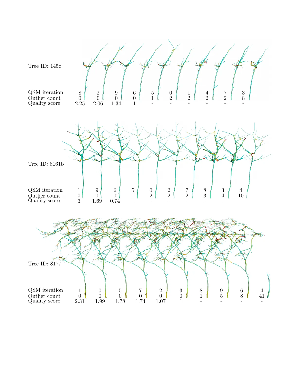
Assessing 3D T ree Mo del Qualit y and Sp ecies Classification Using Im balance Indices Sophie J. Kersting ∗ 1 and Mareik e Fischer † 1 1 Institute of Mathematics and Computer Science, Univ ersity of Greifsw ald, Greifsw ald, Germany Abstract W e in vestigate the use of additional 3D and ph ylogenetic non-3D tree balance indices for analyzing and monitoring forests using an exemplary “virtual forest” dataset from the Wytham W o o ds, Oxford, UK. This study assesses 3D mo del quality , sp ecies classification performance, and the relev ance of these indices. Our study sho ws that indices stemming from the study of ancestry trees of species can b e successfully applied to 3D models of organic trees and, accompanied with recently introduced 3D imbalance indices, offer a complementary p erspective on 3D tree models and impro ve the detection of deviations. Their computational efficiency combined with the simple and reproducible workflo w presen ted in this man uscript form a computationally feasible qualit y con trol step in the 3D model construction. Sp ecies classification models reac hed an estimated accuracy of up to 81.8% and allo wed to mak e confident sp ecies predictions for a large p ortion of the unlab eled trees in the dataset. While con ven tional tree metrics can already provide strong predictive p erformance, the addition of filtered 3D and non-3D statistics improv ed results consisten tly , particularly for minorit y species classes. Alongside this man uscript, we provide up dated functionality in the R pack age treeDbalance to include the necessary functionalities and release the derived index datasets and species predictions. Keywor ds: 3D mo dels, tree balance, plan t architecture, plan t shap e parameters, species classification 1 In tro duction Plan t arc hitecture, esp ecially the branching structure of trees, contains v aluable information about the plan ts’ devel- opmen t, health, and environmen tal in teractions [2, 21, 28, 29, 38, 41]. In the context of climate c hange, high-qualit y estimates of stored CO 2 , the monitoring of tree health, and the study of adaptive resp onses to heat and drought are b ecoming increasingly imp ortant, where the 3D architecture of trees pro vide key structural indicators for these analyses. T o address one asp ect of 3D plant architecture, a set of 3D imbalance indices w as recen tly in troduced that can measure asymmetry in so-called ro oted 3D tree mo dels by considering subtree centroids and gro wth directions [23]. These 3D indices were inspired by physical pendulum mo dels and can quantify both “external” imbalance describing how muc h the plant has gro wn unev enly with resp ect to the horizontal plane, i.e., how muc h the whole plan t leans to one side, as well as “in ternal” imbalance characterizing ho w irregular, crooked, and t wisted the plan t’s v arious parts hav e grown. F urthermore, in the literature there exists a multitude of top ological (im)balance indices from phylogenetics (see [12] for an ov erview of at least 30 (families of ) indices), which disregard spatial orientation and fo cus on the branc hing patterns alone. In this study , we apply the div erse range of 3D and non-3D tree balance indices (all ha v e linear computation time) to a large dataset of 3D tree mo dels from a “virtual forest” dataset from the Wytham W o ods, Oxford, UK [7]. Each tree is represen ted b y ten alternative 3D tree model reconstructions (QSMs), allowing us to assess the consistency of QSM reconstruction and the indices’ sensitivit y to QSM reconstruction v ariation. W e pursue three key questions: 1. Can deviating index v alues across reconstructions indicate flaws and uncertaint y in the QSM reconstruction and guide the selection of the most representativ e QSM p er tree? 2. Can balance indices help infer the sp ecies identit y of trees lab eled “Unknown”, and how big is the impact of the addition of 3D and non-3D indices? ∗ sophie.kersting@uni- greifswald.de † Corresponding author: mareike.fischer@uni- greifswald.de, email@mareikefischer.de 1 3. Which indices contribute most strongly to these tasks and what insights can b e drawn from their relations and comparativ e p erformance? T o this end, we up dated our op enly-a v ailable R pack age treeDbalance to include functionalit y for transforming QSMs into ro oted 3D trees, allo wing the application of 3D imbalance indices, as w ell as extracting the corresponding top ological trees, allowing the application of standard (im)balance indices. W e combine this with statistical and mac hine learning techniques to assess 3D tree mo del robustness, p erform sp ecies classification, and ev aluate index imp ortance. Analyzing the consistency of the ten QSMs per tree pro vided the necessary information to sort out “fault y” QSMs and ultimately select a “b est” QSM for each tree. This uncov ered common construction errors that can b e confirmed with the naked eye, but also error patterns captured by some new indices that cannot b e iden tified, e.g., by the computationally in volv ed comparison with the corresp onding point cloud. T raining random forest and gradient b oosting mo dels allow ed to make confident sp ecies predictions for a large p ortion of trees with unkno wn sp ecies lab el. While the addition of the 3D and non-3D statistics improv ed this p erformance consisten tly when filtered for redundancy , commonly used tree statistics (DBH, height, volume, cro wn area, etc.) can already form the basis for sufficiently well p erforming mo dels. The resulting datasets of index v alues and other statistics of the QSMs, as well as the sp ecies predictions hav e b een made av ailable at h t tp s : //github.com/SophieKersting/SupplementaryMaterial/blob/main/WW_QSMquality_SpeciesClass . The man uscript is structured as follows: Section 2 in tro duces the Wytham W o ods dataset and describes the QSM- to-ro oted-3D-tree-model conv ersion pip eline, follow ed by explanations regarding the indices/statistics and metho ds emplo yed. In Section 3, we present our findings on QSM quality , sp ecies classification, and importance of the individual statistics. Section 4 discusses the implications of these results, and concludes with ideas for future research. App endix A provides an ov erview of the new additions to the softw are pack age treeDbalance while App endix B con tains additional tables and figures. 2 Materials and Metho ds This section provides all necessary information on the data used for this study , including explanations of the (3D) tree mo del formats and statistics that can b e derived from those as well as a description of the workflo w that pro duced the final dataset, but also a list of metho ds used for the v arious research questions. Since the main fo cus of the present manuscript lies in the ev aluation of the dataset rather than in the mathematical details of the individual tree mo del formats and features/statistics, w e keep their descriptions and lists as simple as p ossible, using only the most essen tial mathematical notations. The next paragraphs summarize the formats as w ell as the whole data collection pro cess, en tailed by the statistics and methods. 2.1 The Wytham W o o ds dataset W e used a “virtual forest” dataset whic h w as made av ailable alongside a study by Calders et al. [7] rev ealing that curren t standard es timates potentially underestimate the biomass and b ound CO 2 in temp erate forests. It contains 3D mo dels of the trees inside a 1.4-ha study area lo cated within Wytham W o o ds, Oxford, UK, derived from 3D p oin t clouds with the softw are T reeQSM [5, 37]. These point clouds were created from terrestrial laser scanning (TLS) – a technique which captures the 3D shap es of tree s by emitting millions of laser pulses and measuring the time differences betw een the emission and the detection of the reflected pulses [6]. The dataset co vers 876 trees of 6 differen t sp ecies and provides ten 3D mo dels (QSMs) p er tree sp ecimen (see Figure 2.1). This enables us to assess b oth in tra-tree v ariability and in ter-sp ecies differences. W e used information about the given QSM mo dels while also transforming them into t wo differen t formats which allow us to compute further statistics that provide information ab out the 3D and non-3D im balance of the tree mo dels. 2.2 The three different tree mo del formats This section provides an ov erview of the three tree formats that were in vestigated. More information on how these formats are related and can b e transformed into one another can b e found in Appendix A (Figures A.1 and A.2 pro vide a quick summary). Quan titative structure mo dels (QSMs): The 3D tree mo dels of [7] are given as quantitativ e structure models (QSMs), a widely-used 3D model format that uses cylinders to represent tree branc hes and also stores the information on how these are connected [7, 15, 16, 37]. These QSMs w ere derived from terrestrial laser scanning data and provide 2 T ree ID: 180b 876 trees in total 0 1 2 3 4 5 6 7 8 9 180a 180b 1.7 m Figure 2.1: A visualization of the dataset and the workflo w: Each tree has ten different 3D tree mo dels (in the format of a QSM or a ro oted 3D tree mo del) as w ell as the ten corresponding extracted non-3D top ologies, here exemplarily depicted for the sycamore (A CERPS) with ID 180b. The ro oted 3D trees are colored according to their in ternal A im balance (see Section 2.3.3), where lighter blue colors show lo w and darker red tones higher imbalance. This helps to highlight some common flaws/uncertain ties of QSMs: cylinders forming a bend/angle in the stem (e.g. 180b 7 ), protruding and non-connecting cylinders (e.g. 180b 3 and 180b 4 ) or the absence of certain tree parts (e.g. 180b 0 ). This example was chosen since it is still small and clear (height of ≈ 3 . 5 m and 9 to 14 tips/leav es in the non-3D top ologies) in con trast to the av erage tree height ( ≈ 14 m) and av erage num ber of leav es (791) in the dataset. T ree 180b has a sister stem 180a (heigh t ≈ 25 . 3 m, with around 1526 leav es). Both are depicted on the left side with a h uman figure for scale. This also explains why 180b is leaning to the side / has a high external im balance. In the QSM quality assessment process, 180b 2 w as c hosen as the b est and 180b 9 as the worst QSM (QSM iterations 2, 6, 5, and 4 ∈ B 180b w ere candidates for the b est QSM, while 1, 7, 8, 3, 0, and 9 were filtered out in the negative selection since they each w ere outlier-QSMs for 1 to 11 statistics). precise digital representations of the individual trees. The Wytham W o ods dataset contains 10 QSMs each for 876 tree sp ecimens, and th us, 8,760 QSMs in total. The already published datasets on these 3D tree mo dels range from sp ecies, location, trunk diameter at breast height, heigh t of the tree, estimation of the crown area, total volume, to estimations of the volume of tree parts of certain diameters. (Graph-theoretical) ro oted 3D trees In this present study , these QSMs were transformed into so-called ro oted 3D trees, i.e., ro oted graph-theoretical trees with vertices that hav e 3D coordinates and edges with v olume/thickness [23]. This format holds similar information as a QSM while focusing more on the graph-theoretical branching structure. Th us, conv erting a QSM in to a ro oted 3D tree is straigh tforward without loss of branc hing information (see Figure A.1). Given the ro oted 3D trees, the external and internal im balance of the trees can b e measured. As there are only formal differences b et w een QSMs and ro oted 3D tree s, they cannot b e visually distinguished. Thus, the 3D tree mo dels depicted in Figure 2.1 in the top row can be interpreted b oth as depictions of QSMs or ro oted 3D trees. In order to understand the details of the 3D imbalance statistics in Section 2.3.3 and non-3D statistics in Sec- tion 2.3.4, w e next provide the precise mathematical definitions of ro oted 3D trees and the most crucial concepts, b eginning with some general notes: 3 A (graph-theoretical) r o ote d tr e e or top olo gy 1 is a connected directed graph T with finite vertex/no de set V ( T ) and e dge set E ( T ) ⊆ V ( T ) 2 , containing precisely one vertex, called the r o ot and denoted ρ , such that all edges are directed a wa y from the ro ot. The degree of a v ertex is the num b er of incident edges, consisting of the incoming edges, yielding the in-de gr e e , and the edges leaving the vertex, yielding the out-de gr e e . The ro ot is the only vertex with in-degree 0. Moreov er, there are no v ertices with in-degree > 1. The le af /tip set, which is denoted by V L ( T ), is the set of all nodes in T that hav e out-degree 0, and n is used to refer to its cardinality , i.e., n = | V L ( T ) | . The set of inner vertic es , denoted by ˚ V ( T ), is the set of all v ertices with out-degree ≥ 1, i.e., ˚ V ( T ) = V ( T ) \ V L ( T ). Note that | V ( T ) | = 1 is the only case where the ro ot is the only vertex in the tree and thus also a leaf. F or | V ( T ) | ≥ 2, the ro ot is an inner v ertex. The neighb ors/adjac ent vertices of a no de v are all vertices that connected with v by its inciden t edges. The ro ot-induced partial order on the v ertices (stemming from all edges b eing directed a w ay from the root) allows us to refer to a neigh b or of a v ertex v , as its p ar ent p ( v ) if it is closer to the root than v or as its child otherwise. Whenever there exists a directed path from a vertex u to a v ertex v , we say that u is an anc estor of v and v is a desc endant of u (a no de is its o wn ancestor/descendan t). chil dr en ( v ) and descs ( v ) of a vertex v refer to the set of its c hildren and the set of all its descendan t vertices, resp ectiv ely . n v denotes the n um b er of descending lea ves of vertex v . The depth δ T ( v ) of a v ertex v is its distance to the ro ot measured as the num ber of edges on the unique path from the ro ot to v . The width w T ( d ) of tree T at a given depth d is the num ber of v ertices at depth d , and the height of a tree is the maximal depth of its leav es: h ( T ) = max l ∈ V L ( T ) δ T ( l ). By T v w e denote the p ending subtr e e of a rooted tree T ro oted in v , i.e., T v consists of all of v ’s descendants (includes v itself ) and all edges connecting them. The last/lowest c ommon anc estor LC A ( u, v ) of t w o v ertices u and v is the unique vertex in the in tersection of b oth v ertices’ respective set of ancestors – their common ancestors – with greatest depth. Two leav es, sa y x, y ∈ V L ( T ) are said to form a cherry if they ha ve the same paren t. Similarly , the unique tree with n lea ves is also called a c herry tree. No w, a r o ote d 3D tr e e T = ( T , w ) is a pair consisting of a ro oted tree T = ( V , E ), the top ology , in whic h V ( T ) is a subset of R 3 , i.e., eac h vertex v is a distinct p oin t in the three dimensional space, com bined with a w eight function w that assigns a weigh t w ( e ) to each edge e ∈ E ( T ). Dep ending on the application, the weigh t of an edge e is typically its volume or its physical heaviness, i.e., volume m ultiplied b y density . Similar to non-3D trees, a p ending subtree T v = ( T v , w | E ( T v ) ) consists of the top ology T v and the w eight function restricted to the edges in T v , suc h that T v is again a 3D tree. Non-3D topol ogy F rom ro oted 3D trees w e can extract their non-3D top ologies, which only k eeps their branc hing structure but drops all information on the 3D p ositions and weigh ts of the edges (see Figure A.2). This allo ws us to fo cus on this structural asp ect alone and to apply top ological imbalance indices, which were initially inv ented and used in fields lik e phylogenetics and population genetics. Figure 2.1 in the b ottom ro w exemplarily sho ws extracted non-3D top ologies. In the extraction pro cess, the 3D co ordinate information is dropp ed, an y “stem” consisting of a path from the ro ot to the first branching vertex is remov ed, and other non-branc hing inner vertices are suppressed (see App endix A). Thus, an extracted non-3D top ology T ∗ from a rooted 3D tree T = ( T , w ) is a rooted tree whose v ertices are not p oin ts in 3D space an ymore and which do es not contain v ertices of b oth in- and out-degree 1, i.e., all inner no des ha ve at least 2 c hildren each. 2.3 Statistics This section gives an ov erview of all statistics this study is based on – statistics of the trees, their individual QSMs as well as their corresp onding rooted 3D trees and non-3D top ologies: Those show cased in the lists are used to address at least one of the research questions. All others, i.e., statistics that were omitted or replaced as explained in Section 2.4, are only mentioned in the text. Eac h feature is giv en an abbreviated name (in b old letters) to be used in the figures throughout this manuscript. T able B.1 pro vides a comprehensive summary of the features, including their names in the (original) csv-files and their usage in this manuscript (remo ved, replaced, or used to address one of the researc h questions). 2.3.1 General features First, we go o ver some general features of the trees that are not directly connected to the 3D tree mo del (given in the analysis and figures directory of the supplementary material of [7], and there mainly in the tls summary.csv file): 1 In the main part of this manuscript, apart from the mathematical definitions, we will primarily use the term top olo gy to reduce confusion with the actual trees. 4 Ev ery tree (and its corresp onding point cloud) has a unique T ree ID , and the 10 different QSM v ersions corre- sp onding to the tree are indicated b y a num ber ranging from 0-9, their QSM iteration num b er. Throughout this man uscript we refer to a specific QSM of a tree with ID iteration , e.g., 60 4 for the QSM n umber 4 of the tree with ID 60. Several trees in the study area of the Wytham W o ods consisted of multiple stems and the stems were treated as individual trees if the split into single stems occurred b elo w 1.3 m [7]. These individual stem-trees ha ve the same ID n um b er follo w ed b y a letter, e.g., 180a and 180b (see Figure 2.1). Thus, we introduced the statistic StemCount – the num b er of suc h “sister”-stems in the tree. F urthermore, w e kno w for eac h tree sp ecimen its stem’s precise lo cation ( Locx and Lo cy , i.e., x- and y-co ordinate) in the rectangular study area in the Wytham W o o ds [7]. Of the 876 trees only 835 w ere actually regarded as “inside” of this study area, i.e., at least half of their stem was inside the boundaries. F or these trees – the census trees – there is more information av ailable (called census data in [7], see trees summary.csv ): A manual measurement of the diameter at breast height ( DBHc ) whic h will b e used to assess the v alidity of the QSMs (av ailable for only 695 trees), as well as the Sp ecies of each tree and whether eac h tree was aliv e or Dead at the time of inv estigation (815 alive, 20 dead). The tree species of the 835 census trees – including their n umber of trees N in the dataset as w ell as their Latin name and abbreviations in capital letters – range from field maple (N=2, ACER CAmp estre), sycamore (N=541, A CER PSeudoplatanus), common hazel (N=67, COR Ylus A V ellana), common hawthorn (N=26, CRA T aegus MOnog- yna), European/common ash (N=85, FRAXinus EXcelsior), to p edunculate/English oak (N=37, QUERcus RObur) 2 . 78 trees (71 living + 7 dead sp ecimens) of the 835 census trees could not b e assigned a sp ecies [7, p. 4]. Combined with the 41 remaining non-census trees for whic h no species information is av ailable, this yields 119 trees with species lab el “unkno wn” (see Figure 2.2). Apart from these tw o features, Dead and Sp ecies, all other information is a v ailable for all trees. Thus, there is no further difference b et w een the 835 census trees and the 41 other trees in our study . Figure 2.2: Sp ecies distribution across tree height. The barplot in the bac kground sho ws the total n um b er of trees p er heigh t class and the points the resp ectiv e num bers for the individual sp ecies. The p oin ts are shap ed as the leav es of the corresponding tree species and are only depicted for v alues > 0. The legend also pro vides the respective total n umber of trees p er sp ecies (N). The colors for the sp ecies are the same as in [7, e.g., Fig. 4] to allow easy transfer b et w een visualized results b etw een both studies. 2 At least 23 tree sp ecies hav e b een recorded in the larger 18-ha long-term forest inv entory plot of the Wytham W o ods run by Oxford Universit y [4], but only these six species hav e b een identified in the scanned 1.4-ha area within the larger plot. 5 2.3.2 QSM statistics Regarding features of the actual 3D mo dels of the trees, many were already pro vided in the tls summary.csv of [7]. The downside of these features is that they hav e b een av eraged ov er all ten QSMs p er tree sp ecimen (or hav e only b een estimated from the tree’s TLS p oin t cloud) and as such do not displa y an y v ariation b etw een different QSMs of the same tree and, thus, could not b e used regarding the first key question of this man uscript: ev aluating the qualit y of the QSMs with the goal of finding a “b est” QSM for each tree. Th us, we recalculated all statistics for which it w as p ossible p er QSM from the rooted 3D tree mo dels (see second list below). The following list contains all existing features used in this present study that show no differences b et ween QSMs of the same tree. Each feature is given an abbreviated name to b e used in the figures throughout this man uscript. DBHsd Standard deviation of trunk diameter at breast height (that is at 1.3 m) in m o ver all 10 QSM. Cro wnArea : Estimated area of the crown in m 2 . V olsd : Standard deviation of total volume in m 3 o ver all 10 QSM iterations. V ol0-25sd, etc. : Standard deviation of total v olume of QSM parts/cylinders with a diameter b et ween 0 and 25mm in m 3 o ver all 10 QSM iterations. Similar statistics exist for the diameter ranges 25-50 mm, 50-75 mm, 75-100 mm, 100-200 mm. The census DBH measurement ( DBH census m ) and three further estimations of the DBH from the TLS p oin t clouds ( DBH TLS m and DBH pts m ) and the QSM av erages ( DBH QSM avg m ), as well as a tree heigh t estimation from the TLS p oint clouds ( Hgt pts m ), a volume estimation a veraged ov er all QSMs ( Vol QSM avg m3 ), and volume estimations of QSM parts with a certain diameter av eraged o ver all QSMs ( Vol QSM D0 25 avg m3 etc.) were replaced b y the QSM-sp ecific recomputed statistics as listed b elo w. The following list con tains the features that were recalculated (in cases where only the a verage o ver all QSMs is kno wn) or additionally computed p er QSM. F rom this p oin t onw ard in Section 2.3, all features are QSM-sp e cific . DBH Diameter of the main stem of the QSM at breast height in m. Heigh t Height of the tree (model) in m (difference b et w een maximal and minimal z -co ordinates in the QSM). V olume T otal volume of the tree (model) in m 2 (v olume of all cylinders in the QSM). V ol0-25, etc. : T otal v olume of QSM cylinders with a diameter b et ween 0 and 25 mm in m 3 . Similar statistics exist for the diameter ranges 25-50 mm, 50-75 mm, 75-100 mm, 100-200 mm, and > 200 mm. Length Summed up length of all branches in the tree (mo del) in m (length of all QSM cylinders and connecting branc hes). ZeroCyl The num ber of cylinders in the 3D tree mo del with zero weigh t/volume. A cylinder has zero weigh t or v olume if it has no length or no radius. 2.3.3 3D imbalance statistics Sev eral 3D im balance statistics measuring the in ternal and external balance w ere computed from the rooted 3D trees. The final selection of 3D measures used in this study is: Ext(A)(A/alpha/M/m u) External imbalance, i.e., ho w far the tree leans to the side, as measured by differen t approac hes: The root’s c entr oid angle A ( ρ ) calculates the angle A ( ρ ) : = ∠ ( C ( T ) − ρ, (0 , 0 , 1) t ) b et ween the line from the base of the stem (the “ro ot” of the ro oted 3D tree) to the centroid of the tree and the vertical axis. With the minimal c entr oid angle approach we hav e α ( ρ ) : = A T ,e v ( v ) if 0 ≤ A ( ρ ) ≤ π 2 = 90 ° and π − A ( ρ ) if π 2 < A ( ρ ) ≤ π = 180 ° . The r elative c entr oid distanc e yields µ ( ρ ) : = d ( C ( T ) ,g ver t ) d ( C ( T ) ,ρ ) , where g v ert is the v ertical line going through the ro ot ρ , and the exp ande d r elative c entr oid distanc e yields M ( ρ ) : = µ ( ρ ) if 0 ≤ A ( ρ ) ≤ π 2 = 90 ° and 2 − µ ( ρ ) if π 2 < A ( ρ ) ≤ π = 180 ° . In t-w(A)(A/alpha/M/mu) Internal im balance as measured by a weigh t-w eighted integral-based index using dif- feren t imbalance measuring approac hes: The centroid angle yields the index e A w , which calculates the a v erage 3D im balance ov er the volume (“weigh ts” of the edges) of the tree, where the 3D im balance at a certain p oint v of a branch is measured similarly to the external im balance: It is the angle b et ween the branch leading up to this p oin t and the line to the cen troid 6 C ( T v ) of the part of the tree that starts from there. The formal definition is as follows: Let T = (( V , E ) , w ) b e a rooted 3D tree, then e A w ( T ) : = 0 if | V | = 1 and otherwise e A w ( T ) : = 1 P v ∈ V \{ ρ } w ( e v ) X v ∈ V \{ ρ }  w ( e v ) · Z 1 0 A T ,e v ( v + ( p ( v ) − v ) · x ) d x  , where e v = ( p ( v ) , v ) denotes the incoming edge of v and A T ,e v : V ( T ) \ { ρ } → [0 , π ] is the c entr oid angle of a no de v  = ρ (or edge subdivision) defined as A T ,e v ( v ) : = 0 if C ( T v ) = v and otherwise as the angle A T ,e v ( v ) : = ∠ ( C ( T v ) − v , v − p ( v )). Indices e α w , f M w , and e µ w for the other approaches are formed analogously by exchanging A T ,e v in the form ula ab o v e: If C ( T v )  = v , the minimal c entr oid angle is α T ,e v ( v ) : = A T ,e v ( v ) if 0 ≤ A T ,e v ( v ) ≤ π 2 and π − A T ,e v ( v ) if π 2 < A T ,e v ( v ) ≤ π , the relative cen troid distance is µ T ,e v ( v ) : = d ( C ( T v ) ,g v,p ( v ) ) d ( C ( T v ) ,v ) , with d being the Euclidean distance and g v ,p ( v ) the line v + λ ( p ( v ) − v ) with λ ∈ R going through v and p ( v ), and the expanded relative cen troid distance is M T ,e v ( v ) : = µ T ,e v ( v ) if 0 ≤ A T ,e v ( v ) ≤ π 2 and 2 − µ T ,e v ( v ) if π 2 < A T ,e v ( v ) ≤ π . All three measures are 0 if C ( T v ) = v . In t-l(m)(A/alpha/M/mu) Internal imbalance as measured by a length-w eighted integral-based index using dif- feren t imbalance measuring approaches. These indices are structurally similar to In t-w(A) but differ in the w eighting metho d. Exemplarily , for the cen troid angle based index e A ℓ w e hav e e A ℓ ( T ) : = 0 if | V | = 1 and otherwise e A ℓ ( T ) : = 1 P v ∈ V \{ ρ } ℓ ( e v ) X v ∈ V \{ ρ }  ℓ ( e v ) · Z 1 0 A T ,e v ( v + ( p ( v ) − v ) · x ) d x  . Indices e α ℓ , f M ℓ , and e µ ℓ for the other three approaches are formed analogously by exchanging µ T ,e v in the form ula ab o ve. 2.3.4 T op ological/non-3D statistics This section pro vides information on all statistics deriv ed from the extracted non-3D top ologies. Although the features are known as “tree shap e statistics” or “tree balance indices”, we use the terms “non-3D” or “top ological statistics” to a void confusion with the actual biological trees. As basic top ological features, the n umber of leav es/tips n = | V L ( T ) | (LeafN) and the num b er of inner vertices | ˚ V ( T ) | (InnerN) in the top ology T were collected. Since both highly correlated with other statistics, their ratio was in tro duced as a measure of the resolution of the tree, i.e., ho w little m ultifurcating nodes there are. n − 1 is the maximal n umber of inner vertices (reac hed in a fully binary tree). T opRes The top ological resolution based on the ratio | ˚ V ( T ) | ( n − 1) of the num b er of inner v ertices and the maximal p ossible n um b er of inner vertices in the topology T . Next, we w ere also in terested in the topological imbalance. Although there is a wide range of tree shape statistics, esp ecially (im)balance indices, for rooted trees in phylogenetics [12], only a subset is applicable to the extracted non- 3D top ologies of the Wytham W o o ds trees (see [12, T able 4.1 & 4.2] for details). Several top ological statistics can only b e applied to strictly binary trees, i.e., trees in which edges/branches can only split up into tw o branches and not more at the same time. How ever, a quic k exploration of the 3D tree mo dels revealed that 98.5% (8,632 of the 8,760 QSMs) contain so-called m ultifurcating vertices indicating points where an edge branches in to more than tw o edges. Therefore, we only applied statistics whic h are also suitable for non-binary trees. These are: ALD The av erage leaf depth [40, 42]: N ( T ) : = 1 n · P l ∈ V L ( T ) δ T ( l ). A VD The av erage vertex depth [3, 13, 19, 20]: AV D ( T ) : = 1 | V ( T ) | · P v ∈ V ( T ) δ T ( v ). B1 The B 1 index [42] is the sum of the recipro cals of the heights of the subtrees of T rooted at inner vertices of T (except for ρ ): B 1 ( T ) : = P v ∈ ˚ V ( T ) \{ ρ } 1 h ( T v ) 7 B2 B 2 index [1, 18, 24, 42]: Shannon-Wiener information function (measures the equitability of the probabilities p l ( T ) of reac hing the leav es l ∈ V L in a tree T when starting at the root and assuming equiprobable branching at eac h inner vertex): B 2 ( T ) : = − P l ∈ V L ( T ) p l · log 2 ( p l ). Cherry The cherry index [32] is defined as the n umber c ( T ) of cherries in the tree: C hI ( T ) : = c ( T ). CLe A Colless-like index C D,f with f = exp and D = mean deviation from the median: A represen tative of the family of Colless-lik e indices [34], which calculate the sum of ( D , f )-balance v alues of the inner vertices of T . This balance v alue of an inner v ertex v is defined as bal D,f ( v ) : = D (∆ f ( T v 1 ) , . . . , ∆ f ( T v k )) ov er the so-called f -sizes of its c hildren v 1 , ..., v k , where ∆ f ( T v i ) : = P v ∈ descs ( v i ) f ( | chil dren ( v ) | ). Then, C D,f ( T ) : = P v ∈ ˚ V ( T ) bal D,f ( v ).. CLln Another Colless-like index [34] with f = ln and D b eing the mean deviation from the median. mD The maximum depth [8] or heigh t of a tree: mD ( T ) : = max l ∈ V L ( T ) δ T ( l ) = max v ∈ V ( T ) δ T ( v ) = h ( T ). mW The maximum width [8]: mW ( T ) : = max i =0 ,...,h ( T ) w T ( i ). mD W The Modified maxim um difference in widths mD W [8, 12] is the maxim um difference in widths of tw o consecutiv e depths: mD W ( T ) : = max i =0 ,...,h ( T ) − 1 w T ( i + 1) − w T ( i ). mW omD The maximum width o ver maximum depth [8] is defined as W /D ( T ) : = mW ( T ) mD ( T ) . mI’ Mean I ′ index I ′ [14, 35]: A represen tative of the family of I -based indices which calculates the mean of the I ′ v v alues o ver all inner vertices v with n v ≥ 4 and exactly tw o children (let ˚ V ≥ 4 , 2 ( T ) denote this set of v ertices). The balance v alue I v measures how uneven the descending leav es are split with regard to the most unev en p ossible split and is defined as I v = n v 1 −⌈ n v 2 ⌉ ( n v − 1) −⌈ n v 2 ⌉ , where v 1 is the child of v with the larger num b er of descendan t leav es n v 1 . The I ′ -correction, I ′ v = I v if n v is o dd and I ′ v = n v − 1 n v · I v else, ensures indep endence from the “tree size” n (under certain basic assumptions). Then, I ′ ( T ) : = 1 | ˚ V ≥ 4 , 2 ( T ) | · P v ∈ ˚ V ≥ 4 , 2 ( T ) I ′ v . mIw Another I -based index, namely the mean I w index [14, 35]: I w ( T ) : = 1 | ˚ V ≥ 4 , 2 ( T ) | · P v ∈ ˚ V ≥ 4 , 2 ( T ) I w v . This uses a differen t correction metho d for the I v -v alues namely forming a w eighted mean: The I w v v alue of a vertex v ∈ ˚ V bin, ≥ 4 is defined as I w v : = w ( I v ) · I v mean v ∈ ˚ V bin, ≥ 4 w ( I v ) with w eights w ( I v ) : =      1 if n v is o dd n v − 1 n v if n v is ev en and I v > 0 2 · ( n v − 1) n v if n v is ev en and I v = 0 . rQi Ro oted quartet index rQI [9] with q i = i : A balance index based on the symmetry of subtrees T | Q induced b y quartets Q (sets of four lea ves). The p ossible tree shapes with four lea ves hav e a weigh t q i that scales with the n umber of automorphisms. Let QC T ( T ∗ ) b e the quartet coun t, the n um b er of quartet-induced subtrees in T of shap e T ∗ , then, rQI ( T ) : = q 0 · QC T ( ) + q 1 · QC T ( ) + q 2 · QC T ( ) + q 3 · QC T ( ) + q 4 · QC T ( ). Sac kin The Sackin index [40, 42] (also kno wn as the total external path length) is defined as S ( T ) : = P l ∈ V L ( T ) δ T ( l ). s-shap e The b s -shap e statistic [3] is the sum of log( n v − 1) o ver all inner v ertices of T : b s ( T ) : = P v ∈ ˚ V ( T ) log( n v − 1). TC T otal cophenetic index Φ [33]: The sum of the cophenetic v alues φ T ( x, y ) of all distinct pairs of leav es of T , where φ T ( x, y ) = δ T ( LC A T ( x, y )) is the depth of the last common ancestor LC A T ( x, y ) of x and y . Then, Φ( T ) : = P { x,y }∈ V L ( T ) 2 x  = y φ T ( x, y ). TIPL The total internal path length [25]: T I P ( T ) : = P v ∈ ˚ V ( T ) δ T ( v ). TPL The total path length [11, 43, 44]: T P L ( T ) : = P v ∈ V ( T ) δ T ( v ) = S ( T ) + T I P ( T ). 8 VLD V ariance of leaf depths σ 2 N [10, 40, 42]: σ 2 N ( T ) : = 1 n · P l ∈ V L ( T )  δ T ( l ) − N ( T )  2 . Detailed definitions and more information on the prop erties of these indices can be found in Fisc her et al. [12]. 2.4 Metho ds and w orkflow This section provides detailed information on the workflo w and the statistical and machine learning metho ds, mainly outlier detection for analyzing the quality and robustness of QSMs as well as random forests and gradient bo osting mo dels for the species classification. 2.4.1 Data collection In a parallelized pro cess using the R pac k age treeDbalance , for eac h tree, eac h of the 10 QSM files was loaded and transformed into the ro oted 3D model format (see Figure 2.1 top ro w). This allow ed for the computation of the 3D im balance statistics (Section 2.3.3) as w ell as several QSM statistics (Section 2.3.2). Then, the non-3D topology of each ro oted 3D mo del w as extracted (see Figure 2.1 b ottom row). Based on this, all non-3D imbalance indices w ere computed (Section 2.3.4). All this was com bined with the existing data by Calders et al. [7] to form an initial complete dataset (see df ww all.csv ). 2.4.2 Data cleaning/preparation (Part I) In this phase, the dataset w as prepared for all subsequent steps yielding df ww prep.csv . All changes from this pro cedure are mark ed in gray in T able B.1. Sev eral non-QSM-specific v ariables of the original datasets of [7] were replaced by recomputed QSM-sp ecific v ariables. This affected 4 DBH measurements, as well as heigh t, volume, and tree part v olume estimations as explained in Section 2.3.2. F urthermore, some sparse or non-informative v ariables were com bined into a new v ariable (V ol200+ as the sum of the volumes ov er the diameter ranges 200-500, 500-1000, and > 1000 mm, where the v alues for the t wo thick est categories were b oth > 0 for only 9% of trees) or omitted if this w as imp ossible. The latter w as the case for the standard deviations of the volumes of thick er tree parts with diameters 500-1000 and > 1000 mm, whic h were both also only non-zero for < 9% of trees. When comparing the pairwise relationships of the v ariables, most had no clear or a rather linear relation. How ev er, t wo statistics, the ro oted quartet index with q i = i (rQi) and the Colless-like index with f = exp (CLe), heavily deviated from this, showing a clear quartic, in the case of rQi, and (at least) quadratic, in the case of CLe, relation with other v ariables. Thus, these tw o v ariables were replaced b y 4thrt-rQi and sqrt-CLe , respectively . The quartic relationship in rQi is not surprising, since the num b er of quartets is quartic related to, for example, the num ber of lea ves in a tree (  n 4  = n ! 4!( n − 4)! = n ( n − 1)( n − 2)( n − 3) 4! ∈ O ( n 4 )). 2.4.3 QSM robustness, quality , and selection In this step, the collec ted data is used to determine the qualit y of the individual QSMs with the aim of ha ving a single “b est” QSM p er tree. F or this, we consider each tree with its 10 QSMs separately . The metho d is explained in detail b elo w, but the general idea is to let every statistic decide p er tree which QSMs are outliers, and then to select the p oten tially most accurate QSM from all QSMs with minimal outlier coun t. The pro cess can b e traced in Figure 3.1 in the results section. F or this task, only the 46 “QSM-sp ecific” statistics which hav e individual v alues p er QSM could be used. Let this set of statistics be denoted by S . This limited the statistics to the re- or newly computed DBH, Height, Length, ZeroCyl, V olume, and the V ol0-25 etc. measurements, as w ell as the 3D and non-3D statistics (see T able B.1). Metho d: Outlier detection and selection of the “b est” QSM The goal in this part of the study was to establish sensible criteria based on the av ailable 46 statistics for the quality of a QSM in comparison to its 9 other v ariants – allo wing us to determine the b est QSM for a tree. Tw o main ideas build the basis: First, w e assume that the QSMs capture the real 3D structure to some degree and that c onsensus b et ween QSMs conv eys some degree of truth, and that deviations from this consensus p oin t to wards flaw ed QSMs. Second, w e assume that the most c ommon err ors in QSMs are the absence of tree parts rather than an insertion of new non-existing parts, as well as improp erly fitted and connected cylinders (cylinder paths making sharp b ends or not b eing smo oth) rather than real zigzag branches in the underlying tree. This second notion arose from the man ual in vestigation of a large n umber of smaller QSMs, in which these t ypical errors b ecame apparent (see Figure 2.1 or 9 also Figure A.3 for examples). Missing tree parts tend to create higher internal 3D im balance in the tree since the “coun terweigh t” for other tree parts is missing (see 180b 1 , 180b 4 , or 180b 7 in Figure 2.1). All in all, the QSM quality assessment process is, th us, partly driv en by a “ma jority v ote” of the QSMs but also b y fav oring QSMs that are fuller – therefore p oten tially more complete than others – and internally more balanced – therefore p oten tially with higher cylinder path quality and without loss of tree parts. F ollowing the first c onsensus notion, w e implemented a negativ e selection . F or each tree, its 10 QSMs were examined to see which of the statistics classified them as outliers. Let id be a tree, then QSM j is considered an outlier according to a statistic s (a s -outlier-QSM), if its v alue s ( id j ) is outside of [ q id,s 0 . 25 − 1 . 5 · I QR id,s , q id,s 0 . 75 + 1 . 5 · I QR ] (b o xplot-outlier criterion), where q id,s 0 . 25 and q id,s 0 . 75 are the quartiles and I QR id,s = q id,s 0 . 75 − q id,s 0 . 25 the in terquartile range of the v alues s ( id 0 ) , . . . , s ( id 9 ). Let the outlier assessement be out s ( id j ) = 1 if s regards QSM id j as an outlier, and = 0 otherwise. In case of missing v alues, i.e., if s ( id j ) could not b e computed (only mI’ and TC were affected by this in cases where the tree was to o “small” with regards to num b er of lea ves and inner vertices), as long as the statistic could b e computed for at least t wo of the ten QSMs p er tree, all QSMs with missing v alues w ere flagged as outliers since this p oin ted to wards erroneously missing tree parts (in accordance with the second c ommon err ors idea). If all ten QSMs’ v alues of a tree were missing, this information was considered consensus and none of the QSMs was considered an outlier, and if only one QSM v alue w as av ailable, this QSM was considered the outlier. Based on this, the outlier c ount o ( id j ) = X s ∈ S out s ( id j ), defined as the n umber of statistics which flagged this sp ecific QSM id j as outlier, w as chosen as the metric for the negativ e selection of the QSMs. In the subsequen t p ositiv e selection only QSM v ersions of a tree id with o -ratings = min j =0 ,..., 9 { o ( id j ) } are considered. Let B id ⊆ { 0 , . . . , 9 } b e the QSM iteration num bers of these minimal outlier count QSMs for a tree id , all other QSMs, the negSel-QSMs, are sorted out. Hence, let the negative selection of a QSM b e expressed with neg S M ( id j ) = 0 if j ∈ B id for the metho d M , and = 1 otherwise. Then, the QSM qualit y is determined based on three statistics: on the v olume of smaller tree parts (V ol0-25, V ol25-50) and the in ternal 3D im balance In t-w(A), which was chosen ov er the other internal 3D imablance measures according to the decision tree in [23, Figure 11]. They formed the set S B = { V ol0-25 , V ol25-50 , -Int-w(A) } with the in ternal 3D im balance statistic ha ving a negativ e sign as it had to b e minimized and not maximized lik e the other t w o v olume statistics. As a simple quality criterion whic h uses the quantitativ e information within these three statistics, i.e., how muc h more v olume one QSM has than another etc., w e hav e c hosen the follo wing formula (given a QSM id j with j ∈ B id ) q uality ( id j ) : = X s ∈ S B  s ( id j ) − min b ∈ B id s ( id b ) max b ∈ B id s ( id b ) − min b ∈ B id s ( id b )  , whic h maps the v alues of eac h statistic to the interv al [0 , 1] and then takes the sum o ver the three v alues p er QSM. In the case of max = min for a set of QSMs for a statistic, the corresp onding summand w as set to 0. The “b est” QSM for a given tree is then the QSM whic h has the maximal q uality -v alue among all QSMs id b with b ∈ B id (there w ere no ties). The resulting assignment of T ree ID to the b est QSM (with the additional outlier information) can b e found in df QSMiteration quality.csv . F or the next steps, a dataset that only contains the b est QSM per tree ( df ww 1QSM perTree.csv ) w as extracted from df ww prep.csv . Metho d ev aluation Simple indicators of the qualit y/structure of the metho d explained ab o ve (and v ariations of it) are the negSel-QSM counts p er tree, i.e., the num b er of QMS of a tree that were remo ved in the negativ e selection, as w ell as the num b er of rejecting statistics p er QSM. T o put it precisely , the ne gSel-QSM c ount of a tree id is defined as neg S QC ( id ) = P j ∈{ 0 , ··· , 9 } neg S M ( id j ) = 10 − | B id | , and the numb er of r eje cting statistics of a QSM id j is RS ( id j ) = P s ∈ S out s ( id j ). The resp ectiv e results for the metho d v ariations are sho wn in T ables 3.1 and 3.2. T o v alidate and assess the quality of the negative selection of the metho d, tw o other av ailable information sources w ere used: the original tree p oin t clouds and the census DBH measurements done b y hand. The original point clouds were consulted to ha ve reliable information on the absence of tree parts in the QSMs. F or the 200 trees sT with the smallest QSM files (see Figure 2.3 for examples), we computed the minimal distance of each p oin t in the 3D p oin t cloud to its nearest QSM cylinder, where the distance is zero if the point lies within the cylinder and, otherwise, it is the distance to the closest p oin t on one of the outer faces of the cylinder. This pro cedure is computationally v ery time exp ensiv e as – in the worst case – all pairwise distances of all cylinders and p oin ts ha ve to b e chec k ed (computations for one p oint can b e stopp ed if one distance to a cylinder is 0). Thus, 10 only a subset of the files was used. How ever, with 2,000 QSMs this is still large enough to draw conclusions. T o pro vide some p erspective on the scale s of data, the smallest QSM file con tains 13 (original QSM-) cylinders and its corresp onding point cloud 1255 p oints while the largest assessed QSM files hav e 500 cylinders and around 28,000 corresp onding points. The ov erall largest files in the dataset con tain around 70,000 cylinders and 5.75 million p oints, whic h would ha ve resulted in up to 400 · 10 9 = 400 billion distance computations. (a) (b) Figure 2.3: Two exemplary point clouds, on the left by themselves, then in the middle with their resp ective “b est” QSM as decided by our metho d, and on the right with a flaw ed QSM. (a) P oint cloud of tree 180b consisting of 3,803 points, with QSMs 180b 2 (b est) and 180b 8 with 63 and 42 cylinders, resp ectiv ely . (b) Poin t cloud of tree 145c consisting of 3,039 points, with QSMs 145c 8 (b est) and 145c 5 with 66 and 73 cylinders, resp ectiv ely . The QSMs are colored according to their internal A im balance (see Section 2.3.3). Studying individual trees with QSMs that are known to lack tree parts (see, e.g., 180b and 145c in Figure 2.3) rev ealed that sev eral statistics of these minimal p oin t-cylinder distances are meaningful indicators of missing tree parts in a QSM id j . F or example, the 90 or 95%-quan tiles or the fraction of p oin ts with minimal p oin t-cylinder distances > 0 . 1m= 10cm ( R md> 0 . 1 ( id j )). The decision fell on the latter to ev aluate different method versions as its meaning of distances > 10cm can b e directly understoo d. The fraction is tied to the size of the tree mo del: the bigger the tree, the larger the missing tree part has to b e to hav e the same impact on the v alue. How ever, w e only do comparisons within the R md> 0 . 1 ( id j ) v alues based on the same p oint cloud and thereb y iden tify QSMs with high v alues that indicate incompleteness. The aim was to build a set of true-p ositiv e QSMs (flaw ed QSMs that should b e remo ved in the negativ e selection) and measure which fraction of these are identified during the negative selection. In detail, suc h true-p ositiv e QSMs w ere set as the QSMs with a higher v alue R md> 0 . 1 ( id j ) > q id,R md> 0 . 1 0 . 75 + 0 . 5 · I QR id,R md> 0 . 1 (stricter upp er b ound of the boxplot-outlier-criterion) than the other QSM iterations of the same tree id . As abov e, let the outlier assessemen t b e out R md> 0 . 1 ( id j ) = 1 if R md> 0 . 1 regards QSM id j as an outlier, and = 0 otherwise. T o measure the p oint cloud sensitivity of a method M , we computed the fraction of correctly sorted out PC-outlier-QSMs sens PC ( M ) = P id j ∈ sQ out R md> 0 . 1 ( id j ) · neg S M ( id j ) P id j ∈ sQ out R md> 0 . 1 ( id j ) , where sQ denotes the QSMs of the 200 trees sT with the smallest files in the dataset. This v alue lies betw een 1 (all PC-outlier-QSMs detected) and 0 (none detected). Within this subset of 2,000 QSMs / 200 trees there w ere P id j ∈ sQ out R md> 0 . 1 ( id j ) = 129 PC-outlier-QSMs distributed across 159 trees (41 had no PC-outlier-QSMs). The census DBH measurements w ere used to determine if the a v erage QSMs estimated the correct DBH and with that if the outliers in our metho d were also outliers from the correct DBH. Please note that this information w as not av ailable for all trees, just for 695 of the 835 trees in the census area. In order to build a set of true-p ositiv e QSMs for the census DBH data, the outlier-criterion was adapted and relaxed: out DBHc ( id j ) = 1 if DBH( id j ) ∈ [DBHc( id ) − 2 · I QR id, DBH , DBHc( id ) + 2 · I QR id, DBH ] (DBHc regards QSM id j as an outlier), and = 0 otherwise. T o measure the c ensus DBH sensitivity of a metho d M , we computed 11 the fraction of correctly sorted out census DBH-outlier-QSMs sens DBHc ( M ) = P id j ∈ cQ out DBHc ( id j ) · neg S M ( id j ) P id j ∈ cQ out DBHc ( id j ) , where cQ denotes the set of all QSMs of the 695 census trees cT with a v ailable DBHc data. All in all, among those 6,950 QSMs there were P id j ∈ cQ out DBHc ( id j ) = 3 , 677 DBHc-outlier-QSMs spread across 487 trees (208 had no DBHc-outlier-QSMs). Again, this v alue lies b et ween 1 (all census DBH-outlier-QSMs detected) and 0 (none detected). Unfortunately , the av ailable data do es not give the option to test the precision or sp ecificity of a metho d, i.e., ho w man y true b est QSMs were identified, and w e hav e to settle with measuring whether bad QSMs are correctly sorted out. How ever, we can approac h a kind of Type I I (or β -) error by inv estigating ho w man y best QSMs were in fact PC- or DBHc-outlier-QSMs (# β PC ( M ) and # β DBHc ( M )), which pro vides an understanding if these tw o aspects, whic h can only b e obtained through additional effort (computationally exp ensiv e or manual measuremen ts), can b e correctly accoun ted for with the giv en statistics. T o put these t wo coun ts in to p erspective, w e computed the expected n umber of best QSMs that would hav e b een PC- or DBHc-outliers under tw o simple reference metho ds: The first, Uniform { 0 , . . . , 9 } or U 10 in short, selects each b est QSM uniformly at random from the 10 av ailable ones, i.e., the exp ected num b er is the sum of probabilities to select a PC-outlier-QSM E [# β PC ( U 10 )] = X id ∈ sT P 9 j =0 out R md> 0 . 1 ( id j ) 10 ; analogously for DBHc E [# β DBHc ( U 10 )] = X id ∈ cT P 9 j =0 out DB H c ( id j ) 10 . The second, Uniform B or U B in short, as- sumes that the negative selection (of the main method explained ab ov e) w as correct and only selects the b est QSM uniformly at random from the remaining QSMs id j with j ∈ B id p er tree id . The corresponding exp ected v alues are E [# β PC ( U B )] = X id ∈ sT P j ∈ B id out R md> 0 . 1 ( id j ) | B id | ) and E [# β DBHc ( U B )] = X id ∈ cT P j ∈ B id out DB H c ( id j ) | B id | . If these counts # β PC and # β DBHc are smaller than the counts of the reference mo dels, the metho d M is less, and if larger, more lik ely to choose a “faulty” PC- or DBHc-outlier-QSM as b est QSM. Statistics and their imp ortance Since the negative selection for this dataset is mostly based on a true-false- assessmen t (whether a statistic was flagged as an outsider by at least one statistic) rather than letting the outlier coun t ha ve a gradual influence, similarities of the statistics did not affect this selection criterion. If this had not b een the case, similarity of the statistics would hav e had to b e addressed as the outlier count w ould b e affected b y having subsets of statistics coming to similar conclusions. The aim would b e to hav e the outlier decisions come from differen t information sources and not from statistics that generally come to the same conclusion regarding the deviation of a QSM. Ev en so, we – with regard to the third research question concerning the impact and usefulness of the individual statistics – are interested in similarities and replaceability of the statistics for detecting deviating QSMs. Thus, we in tro duced the pairwise a r eplac e ability sc or e or outlier agr e ement r atio whic h could also b e used to filter the statistics for datasets where a quantitativ e influence of the outlier coun t is aimed at. An agreement ratio a ( i, j ) of statistics i and j is the n umber of times j agrees with i that a QSM is an outlier divided b y the total num b er of times i flags a QSM as outlier. The closer a ( i, j ) is to 1, the b etter i can b e replaced b y j as j detects i ’s outliers just as w ell. These scores were computed for all pairs of these 46 QSM-sp ecific statistics as sho wn in Figure B.1. Row i shows ho w well i can be replaced by the other statistics. The minimal replaceabilit y score of 0.018 has mIw with V ol200+ – in other words, V ol200+ catc hes only around 2% of mIw’s detected outliers. T o ev aluate the effect of filtering and with that the impact of the statistics, we created exemplary filtered sets of statistics for different thresholds. The thresholds 0 . 99, 0 . 85, and 0 . 7 were considered, i.e., the filtering remo ves all statistics for whic h at least one other statistic also detected > 99 / 85 / 70% of its outlier-QSMs. By iteratively remo ving the statistic with the highest replaceabilit y score > 0 . 99 / 0 . 85 / 0 . 7 (and highest P j a ( i, j ) in case of ties), the initial 46 statistics were filtered down to subsets (listed below). F urthermore, differen t initial subsets of statistics w ere used, e.g., only QSM statistics or only non-3D statistics, to in vestigate how m uch usable information these t yp es of statistics can bring to the table. The imp ortance of the individual statistics was measured b y the outlier pr o duction O P ( s ) = P id j ∈ Q out s ( id j ), defined as the n umber of QSMs a statistic s flags as outlier with Q b eing the set of all 8,760 QSMs, and the imp act factor I F ( s ) = P id j ∈ Q out s ( id j ) P s ′ ∈ S out s ′ ( id j ) , which takes into account b oth the outlier pro duction as well as the “uniqueness” of the resp ectiv e statistics as it rewards higher v alues if the statistic is one of few that detects a QSM 12 as an outlier. Please note that the impact factor is dep enden t on the set of observed statistics S which v aries in the differen t metho d v ariations. Similar to the ov erall sensitivity scores of the metho d, we can measure each statistic’s sensitivity to detect PC- and DBHc-outlier-QSMs, i.e., sens PC ( s ) = P id j ∈ sQ out R md> 0 . 1 ( id j ) · out s ( id j ) P id j ∈ sQ out R md> 0 . 1 ( id j ) and sens DBHc ( s ) = P id j ∈ cQ out DBHc ( id j ) · out s ( id j ) P id j ∈ cQ out DBHc ( id j ) . Last but not least, the impact factors of the statistics restricted to only PC- or census DBH-outlier-QSMs focuses on ho w uniquely useful a statistic is in detecting precisely these outlier-QSMs. In mathematical terms these impact factors are defined as I F P C ( s ) = P id j ∈ sQ out R md> 0 . 1 ( id j ) · out s ( id j ) P s ′ ∈ S out s ′ ( id j ) and I F DB H c ( s ) = P id j ∈ cQ out DBHc ( id j ) · out s ( id j ) P s ′ ∈ S out s ′ ( id j ) . Ov erall w e tested the following sets of statistics, i.e., instead of S we consider subsets of S , with v arying filtering options yielding differen t v ariations of the metho d (see also T able 3.3). Amongst other subsets, we also built some optimized subsets of statistics that allow comparisons with other subsets of the same sizes (after filtering). all-nofil Based on all statistics with no filtering. All 46 statistics in S : Height, V olume, Length, ZeroCyl, DBH, V ol0-25, V ol25-50, V ol50-75, V ol75-100, V ol100- 200, V ol200+, In t-w(A), Int-w(a), Int-w(M), Int-w(m), In t-l(A), Int-l(a), Int-l(M), Int-l(m), Ext(A), Ext(a), Ext(M), Ext(m), LeafN, InnerN, B1, B2, Cherry , CLln, mD, mW, mDW, mI’, mIw, Sackin, s-shap e, TPL, TC, VLD, ALD, A VD, TIPL, mW omD, 4thrt-rQi, sqrt-CLe, and T opRes. all-fil99 Based on all statistics with filtering out all statistics with a replaceability score > 0 . 99. 43 statistics (Same initial 46 statistics except Ext(A), Ext(a), Ext(M)). all-fil85 Based on all statistics with filtering out all statistics with a replaceability score > 0 . 85. 41 statistics (Same initial 46 statistics except Ext(A), Ext(a), Ext(M), A VD, and Int-w(m)). all-fil70 Based on all statistics with filtering out all statistics with a replaceability score > 0 . 7. 35 statistics (Same initial 46 statistics except Ext(A), Ext(a), Ext(M), A VD, Int-w(m), Int-w(M), In t-w(A), TPL, In t-l(M), Int-l(m), and CLln). onlyQSM = onlyQSM-fil70 Based only on QSM statistics with replaceabilit y filtering threshold 0 . 7. 11 statistics: Height, V olume, Length, ZeroCyl, DBH, V ol0-25, V ol25-50, V ol50-75, V ol75-100, V ol100-200, and V ol200+. only3D-fil70 Based only on 3D imbalance statistics with replaceabilit y filtering threshold 0 . 7. 4 statistics: Int-w(a), In t-l(A), Int-l(a), and Ext(m). onlyNon3D-fil70 Based only on top ological/non-3D statistics with replaceabilit y filtering threshold 0 . 7. 20 statistics: LeafN, InnerN, B1, B2, Cherry , mD, mW, mDW, mI’, mIw, Sac kin, s-shape, TC, VLD, ALD, TIPL, mW omD, 4thrt-rQi, sqrt-CLe, and T opRes. all-NOTQSM-fil70 Based on all but QSM statistics with replaceability filtering threshold 0 . 7. 24 statistics: In t-w(a), Int-l(A), In t-l(a), Ext(m), LeafN, InnerN, B1, B2, Cherry , mD, mW, mDW, mI’, mIw, Sac kin, s-shap e, TC, VLD, ALD, TIPL, mW omD, 4thrt-rQi, sqrt-CLe, and T opRes. all-NOT3D-fil70 Based on all but 3D imbalance statistics with replaceabilit y filtering threshold 0 . 7. 31 statistics: Height, V olume, Length, ZeroCyl, DBH, V ol0-25, V ol25-50, V ol50-75, V ol75-100, V ol100-200, V ol200+, LeafN, InnerN, B1, B2, Cherry , mD, mW, mD W, mI’, mIw, Sackin, s-shap e, TC, VLD, ALD, TIPL, mW omD, 4thrt-rQi, sqrt-CLe, and T opRes. all-NOTnon3D-fil70 Based on all but top ological/non-3D statistics with replaceabilit y filtering threshold 0 . 7. 15 statistics: Height, V olume, Length, ZeroCyl, DBH, V ol0-25, V ol25-50, V ol50-75, V ol75-100, V ol100-200, V ol200+, Int-w(a), In t-l(A), Int-l(a), Ext(m). opt4 Based on four v ariables obtained by a greedy search for the statistics with the highest impact: This searc h pro cess starts with all statistics s ∈ S and computes their impact factors. Then, iterativ ely the statistic with the highest impact factor is chosen as an optimal statistic and the impact factors of all other statistics are recomputed without all QSMs the optimal statistics ha ve already flagged as outliers. This yielded DBH, Heigh t, sqrt-CLe, and B2. opt11 Based on ten v ariables with highest impact, obtained as in opt4. These are DBH, Height, sqrt-CLe, B2, mD W, V ol0-25, V ol50-75, ZeroCyl, mI’, V ol100-200, and V ol25-50. 13 opt15 Based on 15 v ariables with highest impact, obtained as in opt4. These are DBH, Heigh t, sqrt-CLe, B2, mDW, V ol0-25, V ol50-75, ZeroCyl, mI’, V ol100-200, V ol25-50, T opRes, B1, mW, and V ol75-100. 2.4.4 Data cleaning/preparation (Part I I) In this step, the dataset df ww 1QSMperTree.csv was prepared for the sp ecies classification under the name “b est” QSM data (yielding df ww 1QSMperTree prep.csv ). The sparse v ariable ZeroCyl as well as an y standard deviation statistic (DBHsd, V olsd, etc.) were remov ed at this point as they are only a sign of QSM quality without giving information ab out the underlying 3D structure. Some v ariables had missing v alues. These w ere informative for the outlier detection, but would interfere with the sp ecies classification as these statistics would hav e been omitted entirely . Only eight QSMs were affected (1950 2 , 2024a 0 , 2053b 6 , 2316 6 , 532b 6 , 8033 4 , 8171 0 , 8357 5 ), and for these only the statistics mI’ and mIw as w ell as mW omD. In all cases the reason was that the extracted topology was to o small. mI’ and mIw need at least n = 4 leav es in the top ology to b e computable, but all eight extracted top ologies hav e 1-3 leav es. Since the v alues of mI’ and mIw can range b et ween 0 (balanced) and 1 (imbalanced), the v alues were set to 0.5 since there is only one top ology for eac h of these tree sizes. mW omD mW mD cannot b e computed if the maxim um depth mD is zero, which is the case if the non-3D top ology consists of only one (ro ot) vertex, i.e., the 3D mo dels are a single stem without branching. This applies to the trees with IDs 1950 2 , 2316 6 , 532b 6 , 8171 0 , and 8357 5 . W e set the missing mW omD v alues to 2, the v alue of the smallest tree which has a mW omD v alue, the cherry tree with n = 2 leav es, since this v alue is also consisten t with the ranges of mW omD for higher n . 3 2.4.5 Sp ecies classification The goal w as to ev aluate the predictive p o wer of both the original statistics by themselv es and the union of the original and newly introduced statistics for an application example, namely tree species classification. The prediction mo dels w ere trained and ev aluated on the subset of trees for whic h the sp ecies was known, and the resulting models were subsequen tly applied to trees with unknown species lab els. Due to small sample sizes in some species classes, 2 A CERCA, 26 CRA TMO, and 37 QUERR O trees (eac h with few er than 40 observ ations) were merged into a single class, Other, to decrease the high class im balance. The final lab eled data comprised 758 trees with the follo wing sp ecies distribution: ACERPS: 541, COR Y A V: 67, FRAXEX: 85, Other: 65. The unlab eled part of the dataset consists of 118 trees with sp ecies class Unkno wn. Tw o predictor sets w ere ev aluated: i) all 49 av ailable numeric statistics P all and ii) the 12 original numeric statistics P ori (consisting of Lo cx, Locy , DBH, CrownArea, Heigh t, and the v arious volume statistics, see T able B.1 for details). Although random forests are generally robust to multicollinearit y and tend to down-w eigh t redundant predictors, v ariable imp ortance estimates ma y b e diluted when predictors are strongly correlated. In order to make more meaningful statements ab out the imp ortance of individual predictors, an additional iii) filtered predictor set P f ill comprising 17 v ariables w as constructed b y remo ving highly correlated features based on the P earson correlation co efficien t, using a threshold of | r | > 0 . 9 (Figures B.2 and B.3). Pearson correlation w as c hosen o ver rank-based alternativ es (e.g., Spe arman) b ecause the cases of clear non-linear relations (rQi and CLe) were already addressed in Section 2.4.2. General pro cedure Sp ecies classification w as p erformed using t wo methods to assess robustness with resp ect to classifier choice: Random forests (RF) [17, Sec. 15], an ensem ble learning metho d that combines predictions from a large n umber of dec ision trees trained on bo otstrapped samples and random subsets of v ariables, as w ell as gradien t b oosting mo dels (GB) [17, Sec. 10.9], a sequential ensemble approach in whic h trees are combined iteratively to correct the errors of previous ones. T o assess the predictive p erformance of the RF and GB mo dels based on the three predictor sets (while a voiding o verfitting), we used nested cross-v alidation [22, Sec. 5.1]. This was done with the R pack ages randomFo rest [30], gbm [39], and ca ret [27]. This pro cedure consists of t wo loops: An outer loop (10 folds) used for p erformance ev aluation: The labeled dataset is split into 10 subsets. In each iteration, one fold is held out as a test set and the remaining folds are combined, then used for parameter tuning in the inner lo op and as a training set for a final model with optimized parameters whic h is ev aluated on the test set. An inner lo op (5 folds) used for hyperparameter tuning: The training p ortion from the outer lo op is split in to 5 folds. In each iteration, again, one fold is held out for ev aluation and the remaining folds serve as training data for 3 The maximal mW omD v alues for n = 2 , 3 , 4 , 5 , ... are 2 , 3 , 4 , 5 , ... (reached by the “star” topology consisting of the ro ot and otherwise only leaves) and the minim al v alues are 2 n − 1 [12, Cor. 23.4], i.e., for n = 2 the only possible v alue is 2, for n = 3 v alues lie b et ween 1 and 3, for n = 4 b et ween 2 / 3 and 4, for n = 5 b et ween 2 / 4 = 1 / 2 and 5, and so on. 14 eac h hyperparameter configuration. The inner lo op returns the b est parameter setting ov er all iterations according to a p erformance metric, in this case log-loss. The log-loss, in short − 1 t t X i =1 log ( p true ( i )), where t is the num b er of observ ations/trees and p true ( i ) is the prob- abilit y that tree i is assigned its true class, was chosen as an optimization metric. It is more suitable for this case as, for example, the accuracy of the predictions, since it is sensitiv e to minority classes and punishes ov er-confident mistak es. F or instance, a mo del that assigns ACERPS to all trees with certaint y 0.99 would hav e a go o d accuracy of around 71% but extremely high log-loss as p true ( i ) is v ery small for the remaining 29% of trees. Ov erall, this procedure ensures that the final ev aluation on the outer test folds reflects out-of-sample p erformance, a voiding o ver-optimistic estimates that occur if tuning and ev aluation are done on the same data. W e rep ort the following p erformance metrics deriv ed from the p ooled out-of-sample predictions across the test set of the outer folds of the nested cross v alidation (each tree of the dataset app ears exactly once): Accuracy A , the p ercen tage of correctly predicted tree species; Cohen’s κ defined as κ = A − A E 1 − A E , where A E is the expected accuracy b y random guessing giv en the observed class frequencies, to quantify classification agreement beyond chance; log-loss (see ab o v e); class-wise sensitivities; and macro-av eraged sensitivity , i.e., the mean across all class-wise sensitivities. Subsequen tly , a final mo del was trained on the entire predictor and dataset (using the best hyperparameter configuration from the nested cross-v alidation) for the prediction of the unlab eled trees’ species classes. Details on species classification with random forests Exploring a broad range of num b ers of trees ntree in the random forest, the n umber w as fixed at 1,000 as the p erformance plateaus for ≥ 800 trees. The only h yp erparameter for RF is mtry , which determines the size of the subsets of randomly chosen predictors eac h split in each decision tree is allo wed to consider. A small v alue ( ≪ | P ... | ) decreases correlations b et w een the individual decision trees, leading to reduced v ariance and more stable ensemble classification performance. The configurations for tuning w ere { 2 , 3 , . . . , 8 } , which includes the default v alue ≈ p | P ... | , which is b et w een p | P ori | = √ 12 ≈ 3 . 5 and p | P all | = √ 49 = 7 for the three predictor sets. F or the final RF mo del based on | P f il | , the b est performing v ersion, the h yp erparameter mtry was set to 6 – one of the most frequently selected mtry v alues (and relativ ely close to the mean v alue 6 . 8) across the outer folds for this predictor set. The sp ecies classification results with all class probabilities can b e found in species class RF.csv . V ariable imp ortance was assessed using the mean decrease in accuracy , whic h quantifies the reduction in mo del accuracy when the v alues of a giv en predictor are randomly p erm uted while all other predictors are held constan t. Details on species classification with gradient b oosting mo dels (GB) F or GB mo dels there are several h yp erparameters [22, Sec. 8.2.3], which mak es tuning more in volv ed. n.trees con trols the total num b er of sequen tial decision trees that are added and the interaction.depth sp ecifies the n umber of splits 4 in the individual decision trees, while the learning rate ( shrinkage ) manages the con tribution of each individual tree to the ensemble and n.minobsinnode limits the minim um num b er of observ ations p er terminal node. The following tuning configurations w ere used: { 800 , 1 , 000 , 1 , 200 } for n.trees to b e sufficient for common (default) shrinkage v alues { 0 . 1 , 0 . 01 } , { 1 , 2 , 3 } for interaction.depth to capture only main effects and small interactions (reduces prediction v ariance), and { 3 , 5 , 7 } for n.minobsinnode to preven t ov erly sp ecific and unsupp orted splits which reduces ov erfitting and sensitivit y to noise. The most frequently c hosen h yp erparameters in the outer folds whic h w ere used in the final GB mo del based on | P f il | , the b est p erforming version, w ere n.trees = 800, interaction.depth = 3, shrinkage = 0.01, as well as n.minobsinnode =7. species class GB.csv contain the sp ecies predictions with all class probabilities. F or the GB mo dels, v ariable imp ortance was assessed using the built-in metric from the ca ret pac k age, which quan tifies the contribution of eac h predictor to reducing the mo del’s loss function (multinomial deviance, i.e., the negativ e log-likelihoo d of the true class lab els under the predicted probabilities) across all trees in the ensem ble. Data visualization A principal component analysis (PCA) [22, Sec. 10.2], a method that allows summarizing a large set of statistics (here P all ) with a smaller set of representativ e v ariables (linear combinations of the statistics) that collectively explain the most v ariance in the data, was performed on the“b est” QSM data using the R pack age stats [36]. Prior to the PCA, all v ariables were cen tered and scaled to unit v ariance. 4 Each split (binary vertex) in a decision tree represents a decision rule of the form p ≤ c , where a single predictor p and a thresh- old v alue c partition the feature space into tw o disjoint regions (left/righ t child no des). The parameter name here is misleading as interaction.depth does not refer to the decision tree’s depth but to its num b er of inner (binary) vertices. 15 F urthermore, uniform manifold approximation and pro jection (UMAP) [31] was used as a nonlinear embedding [17, Sec. 14.9] for the visualization of the (lo cal) neigh b orhoo d structure of the scaled data in t w o dimensions. UMAP em b eddings were computed using the R pack age umap (version 0.2.10.0) [26] with Euclidean distance, n neighbors = 20 and min dist = 0.1 . A fixed random seed was used to ensure reproducibility . T o assess the contribution of the new 3D and non-3D statistics to the original set of QSM statistics and general features, UMAP embeddings w ere computed for all three sets of statistics i)-iii). In all cases, identical UMAP parameters and random seeds were used, such that differences b et w een embeddings reflect changes in the input feature space rather than tuning of the embedding algorithm. F or b oth, PCA and UMAP , samples w ere colored according to their species class for visualization purp oses only . 3 Results This section discusses the results of this study with regards to the three main research questions regarding 1) the QSM quality , 2) the sp ecies classification as an application example, and 3) the imp ortance and relations of the statistics. 3.1 QSM quality assessmen t The t wo interesting asp ects here are, firstly , what we uncov er ab out the 3D tree mo dels themselves: What are common QSM construction errors, how can they b e detected, and how high is the v ariation b et ween differen t QSM v ersions of one tree? Secondly , the metho d of quality assessment based on the (outliers of the) statistics is ev aluated regarding how w ell it can detect flaws in QSMs and select a “b est” QSM per tree. While discussing the details of these tw o main asp ects, the v alidity of the tw o foundational assumptions, c onsensus and the c ommon err ors , will b e addressed as w ell. Overall, this aims at narr owing do wn ho w an efficient qualit y con trol within the QSM construction pro cess could look like to immediately flag or discard highly fla wed QSMs. Qualit y of the QSMs The most important result is that – in the ov erwhelming ma jorit y of cases – the QSMs are relativ ely w ell fitting mo dels of the 3D structure and, while there are notable qualit y differences, most of the time sev eral of the 10 QSMs p er tree are go o d and non-deviating represen tations of the 3D architecture (see Figures 3.1 or also 2.1). On av erage around 6.6 but alwa ys at least 1 of the 10 QSMs were filtered out in the negative selection (see T able 3.1). This left 3.5 candidates for the “b est” QSMs on av erage, with n umbers ranging b et w een 1 to 6 in most cases. The finally chosen “b est” QSMs p er tree were mostly considered non-deviating by all statistics. 843 of the 876 “b est” QSMs ha ve an outlier coun t of 0, and the remaining 33 only one of 1. Another main discov ery is that the QSM flaws detected within this inv estigation do not hinder the quan titative structure mo dels’ – as the name suggests – primary usage as a foundation for ab o ve-ground v olume and biomass estimations. On the con trary , the findings suggest that the results b y Calders et al. [7] w ere rather conserv ative and p oin t to a slight underestimation of the total volume and with that the biomass. After summarizing these most relev an t results and discov eries, the remainder of this section sho wcases and discusses the more detailed observ ations. Figure 3.1 shows three exemplary trees with the outlier counts and quality scores of their QSMs. Some reasons wh y certain QSMs were filtered out in the negative selection can b e observed there: for example increased internal 3D imbalance in 8177 8 , 8177 9 , and 8177 6 , or missing tree tips in 8161b 8 , 8161b 3 , and 8161b 4 . The results for the sycamore with ID 180b depicted in Figure 2.1 are as follows: QSM iteration 2 is the b est QSM. Iterations 2, 4, 5, and 6 were left after the negative selection whic h sorted out 180b 1 with one, 180b 7 with tw o, 180b 8 with three, 180b 3 with four, 180b 0 with fiv e, and 180b 9 with elev en statistics regarding them as outlier-QSMs. There are cases of total failure, e.g. 8177 4 as shown in Figure 3.1 (c), where next to none of the 3D structure is captured by the QSM cylinders, but these are not t ypical and especially for larger tree models there are no examples of comparable severit y as 8177 4 . F ortunately , many statistics (41 different statistics in case of 8177 4 ) can identify suc h extreme cases as deviating, e.g., V olume which is already commonly computed. Consulting T able 3.2, roughly one third of the QSMs were not considered an outlier-QSM by any statistics, more than one third w as flagged by only 1 or 2 statistics (these could still be considered candidates for the “b est” QSM in a less strict approac h), and around 15% of the QSMs were flagged b y at least 5 statistics. It would b e advisable to emplo y a small set of v ariables at the minimum, so that at least such QSMs, whose assessmen t as an outlier is supp orted b y several or all of them, can b e remov ed or replaced. How ever, the smaller the set of statistics, the stricter and more generalized the filtering turns out. While it could b e discussed to keep QSMs as candidates if only a few statistics identified them as outlier-QSMs as mentioned ab ov e, the usage of the 16 T ree ID: 145c QSM iteration 8 2 9 6 5 0 1 4 7 3 Outlier coun t 0 0 0 0 1 2 2 2 2 8 Qualit y score 2.25 2.06 1.34 1 - - - - - - (a) T ree ID: 8161b QSM iteration 1 9 6 5 0 2 7 8 3 4 Outlier coun t 0 0 0 1 2 2 2 3 4 10 Qualit y score 3 1.69 0.74 - - - - - - - (b) T ree ID: 8177 QSM iteration 1 0 5 7 2 3 8 9 6 4 Outlier coun t 0 0 0 0 0 0 1 5 8 41 Qualit y score 2.31 1.99 1.78 1.74 1.07 1 - - - - (c) Figure 3.1: Exemplary results of the QSM quality assessment for (a) the sycamore (A CERPS) with ID 145c (145c 8 has height 3.42 m, DBH 0.05 m and 16 leav es), (b) the sycamore with ID 8161b (8161b 1 has height 5.26 m, DBH 0.04 m and 23 leav es), and (c) the common hazel (COR Y A V) with ID 8177 (8177 1 has height 5.9 m, DBH 0.06 m and 292 leav es). The QSMs are sorted by outlier coun t and then qualit y score. The QSMs are colored according to their in ternal A imbalance (see Section 2.3.3). 17 T able 3.1: The num b er of trees with the respective negSel-QSM coun ts. The negSel-QSM count of a tree id is the n umber of QSMs neg S QC ( id ) = P j ∈{ 0 , ··· , 9 } neg S M ( id j ) of the tree that w ere filtered out in the negative selection as b eing an outlier for too many statistics and with that w ere no candidates for the b est QSM of id . The last column holds the resp ective mean negSel-QSM counts (rounded to tw o decimal places). F or readability , en tries with 0 are not sho wn. negSel-QSM count 0 1 2 3 4 5 6 7 8 9 Mean all-nofil 1 6 18 56 126 191 199 185 94 6.61 all-fil99 2 5 18 56 126 191 199 186 93 6.60 all-fil85 2 5 18 56 128 193 198 184 92 6.59 all-fil70 2 5 18 65 145 181 203 173 84 6.50 onlyQSM-fil70 26 78 167 189 175 121 81 23 9 7 3.50 only3D-fil70 226 286 214 101 40 8 1 1.40 onlyNon3D-fil70 3 27 69 149 177 190 149 78 29 5 4.55 all-NOTQSM-fil70 11 38 102 176 172 172 127 58 20 5.16 all-NOT3D-fil70 3 8 35 93 153 202 185 130 67 6.18 all-NOTnon3D-fil70 11 27 102 175 206 145 130 59 12 9 4.20 opt4 100 227 243 164 89 42 8 3 2.1 opt11 9 40 128 174 184 162 106 45 20 8 4.05 opt15 3 13 65 117 178 190 159 101 33 17 4.83 opt11 statistics, for instance, flags only around 11% of the QSMs by more than 2 statistics and 30% by 1 statistic (see T able 3.2). This do es not leav e a lot of ro om for deciding on a threshold of rejecting statistics for the negative selection of the most extreme cases, since a threshold of 2 would mean that at least 5 of the 15% the main metho d iden tified as well-supported outlier-QSMs are not remov ed, whereas a threshold of 1 w ould remov e ev en mild cases of deviation (whic h would b e v alid if intended). Therefore, only using the already commonly computed statistics lik e Height and V olume would, at the one hand, already b e extremely helpful to identify a large part of the most hea vily deviating QSMs, but, on the other hand, imply a strict remov al of an y flagged QSMs and not allow for a more relaxed approach to the filtering if that is desired. The addition of 3D and non-3D statistics could give this relaxation option. F urthermore, it w ould gran t the ability to identify v arious other deviation patterns b ecause most statistics – apart from a few subsets lik e Int-l, Int-w, and Ext – ha ve extremely low pairwise replaceabilit y scores, meaning that they capture unique outlier information (see Figure B.1). T able 3.2: The n umber of QSMs with the respective RS coun ts. The num ber of rejecting statistics RS ( id j ) = P s ∈ S out s ( id j ) of a QSM id j coun ts ho w many statistics regard this QSM as an outlier. F or readability , en tries with 0 are not shown. Num. of rejecting statistics 0 1 2 3 4 5 6 7 8 9 10 11 12 13 14 15 16 17 ≥ 18 all-nofil 2857 2146 1224 664 527 363 241 182 134 99 83 60 50 21 20 15 18 14 42 all-fil99 2857 2236 1308 728 480 309 206 161 121 89 69 46 39 22 19 9 15 16 30 all-fil85 2867 2284 1308 754 485 315 188 165 114 69 62 37 28 16 17 16 8 6 21 all-fil70 2944 2378 1439 807 458 277 161 96 65 37 34 24 14 8 7 4 2 1 4 onlyQSM-fil70 5623 2185 634 222 59 19 11 6 1 only3D-fil70 7537 852 280 81 10 onlyNon3D-fil70 4765 2089 902 418 248 139 78 48 41 15 9 2 2 2 1 1 all-NOTQSM-fil70 4228 2194 1071 540 293 166 102 66 38 23 15 12 5 3 2 1 1 all-NOT3D-fil70 3249 2443 1372 717 395 218 125 99 41 37 24 21 6 3 3 2 1 1 3 all-NOTnon3D-fil70 5021 2262 879 342 150 61 24 9 7 3 2 opt4 6920 1662 169 9 opt11 5139 2691 731 160 29 5 3 1 1 opt15 4441 2904 1023 290 76 15 7 1 1 1 1 Apart from these rare notable outliers, there are also several more subtle flaws in some QSMs which could impact their usage for some applications that fo cus more on the details rather than the o v erall volume of the 3D tree models. These are, for example, smaller missing tree parts like the top right branch of tree 180b, which is not represented b y cylinders in QSM iterations four to eigh t (see Figure 2.1). A comparison with the corresp onding p oin t cloud 18 depicted in Figure 2.3 (a) shows that, indeed, these parts are gen uinely absent rather than b eing imagined in the 3D mo del construction of the other QSMs. Because the remaining QSM iterations agree on the branc h’s existence, this pro vides some v alidity to the c onsensus claim. QSM c onsensus can also clear up the more seldom opp osite cases of falsely added branches: The top-most twig of 145c 5 only app ears in this sp ecific QSM shown in Figure 3.1 (a) and no other. Consulting the point cloud (see Figure 2.3 (b)) reveals that this branch, in fact, is not w ell supported and thereb y with great certain ty fault y . This deviation was successfully identified b y the statistic Height, which flagged 145c 5 as an outlier-QSM. While p oten tially problematic for smaller trees, where these parts can mak e up a significant p ortion of the whole structure, larger trees will not be impacted notably by the absence of smaller branches. Another observ ation regarding detailed QSM qualit y , w ere the frequen t cylinder offsets, i.e., the end p oin ts of QSM cylinders not matching or following the same line (see Figure A.3). This prompted us to use a differen t parameter for the transformation in to the ro oted 3D tree format, which allow ed the In t-w indices to ignore the imbalance resulting from the m ulitude of small highly imbalance cylinder connections. Again, this fla w became apparen t but do es not affect most usages. F or some special cases, it might b e of in terest to experiment with running a “smo othing” algorithm along the stems of the 3D tree models to b oth reduce cylinder offsets but also catc h erroneously protruding cylinder p eaks as sho wn in Figure A.3 (a). One of the most practically irrelev ant observ ations is the occurrence of “non-existing” cylinders, cylinders whic h ha ve either no length or nor radius and with that no v olume, as trac ked by the statistic ZeroCyl. These do not affect the 3D tree mo dels usage but are unnecessary information within the model. All in all, the metho d show ed reliable results in deciding on plausible “b est” QSMs p er tree. While the volume of smaller tree parts w as a factor in the p ositiv e selection to choose QSMs with fewer losses of tree parts, the total v olume w as not. When comparing the total volume of the “b est” QSMs, 1104.71m 3 , with the total of a verage v olumes o ver eac h set of ten QSMs, 1092.44m 3 , we see a 1.12% increase. When restricted to only census trees the total v olume increased b y 1.06% from 1054.46 3 to 1065.65 3 through the selection process of “b est” QSMs. This c hange is plausible as we hav e seen examples of considerable losses (8177 4 in Figure 3.1 (c)). Simultaneously the difference is not high enough to attribute a significant bias (fa v oring ov erly voluminous 3D tree models) to the metho d itself. As mentioned at the b eginning of this section, the Wytham W o ods QSM dataset w as used to estimate the ab ov e- ground biomass with the tree volumes a v eraged ov er eac h set of ten QSMs [7]. The fact that the “best” QSMs ha ve a similar or sligh tly higher total volume might indicate that the volume that had b een used as a basis was slightly underestimated and supp orts or probably even strengthens Calders et al. [7]’s result that the widely used allometric mo del underestimates the abov e-ground biomass of a typical UK temperate forest. F or most other statistics, the total a veraged v alues and the total best v alues only differed b y -2.7% to 2.4%, i.e., the selection pro cess did not impact these statistics on a dataset level. F or four statistics the b est-QSM-selection resulted in more significant decreases: ZeroCyl ≈ − 16%, sqrt-CLe ≈ − 11%, TC ≈ − 7%, and VLD ≈ − 6%. The latter three statistics also ha ve high outlier production (see T able 3.6 discussed in more detail in Section 3.3), which could mean that, in particular, QSMs with esp ecially large sqrt-CLe and VLD were negativ ely selected and not c hosen as b est QSM. Ev aluation of the method The entire metho d was based on t wo key assumptions, c onsensus and the c ommon err ors , that are broadly confirmed b y the results. The c onsensus work ed and prev ailed for the manually insp ected trees, as already exemplary discussed for 145c 5 or 6177 4 in Figure 3.1. The comparisons with the p oin t clouds (examples in Figure 2.3) rev ealed that missing branc hes are the most prev alent errors as assumed in the c ommon err ors notion. Most often ev en the b est QSMs do not account for ev ery small twig while w orse QSMs might b e missing larger parts of the structures. Erroneously added tree parts like with 145 5 are extremely rare. Internal imbalance as another common error and also as an indication of the absence of tree parts stemming from a man ual insp ection of smaller example trees has also b een supp orted on a broader scale. One example b eing tree 8177 (see Figure 3.1 (c)) with more and more red colored, i.e., highly im balanced, and less full branc hes the higher the outlier coun t of the corresponding QSMs (except 8177 4 whic h is lacking to o man y branches to ev en b e imbalanced). No w, how well did the metho d do regarding the av ailable p erformance metrics? The main metho d based on all suitable statistics without filtering was able to detect 86% of the QSMs the point cloud statistic R md> 0 . 1 flagged as outlier and 69.2% of the consensus DBH-outlier-QSMs (see T able 3.3). The qualit y and degree of deviation of the DBHc- and PC-outlier-QSMs w as chec k ed on several small examples, amongst others on the four depicted trees in Figure 2.1 and 3.1: The three smaller trees 180b, 145c, and 8161b were within the subset of trees for whic h the QSMs were compared with their p oin t clouds. Thus, we ha v e PC-outlier-QSM information for them: QSM iterations 0 and 8 are PC-outlier-QSMS for 180b, and for 8161b these are 3 and 0 (b oth successfully filtered out in the negative selection for both trees). 145c has no QSMs flagged as outlier by R md> 0 . 1 . Please note that R md> 0 . 1 can only detect the absence and not the faulty addition of branches as, for example, the one in QSM 145c 5 (see Figure 3.1 (a)), 19 since the distances of the p oin ts to their nearest cylinders was recorded. Thus, missing cylinders would lea v e traces in the data where additional cylinders would not. The lack of PC-outlier-QSMs for tree 145c, how ever, aligns with the additional branch b eing incorrect, since otherwise all but QSM 5 would hav e to b e outliers. The tree 8177 is the only one of these four which w as inside the census area. Its DBHc-outlier-QSMs are 2, 5, 8, 0, 3, and 9 (ordered by decreasing DBH), where, in fact, all its QSMs had a DBH low er than the census DBH v alue, but these particular QSMs had the low est v alues. F rom these 6 QSMs only 8 and 9 w ere filtered out in the negative selection but the b est QSM 8177 1 is no DBHc-outlier-QSM. The collected data on the Type I I error coun ts # β PC and # β DBHc sho wn in T able 3.3 also allows to ev aluated the t wo steps, the negativ e selection and the decision on the “b est” QSM according to the quality score, of the process. F or PC, we exp ect around 24 PC-outlier QSMs as “b est” QSM if they w ere chosen at random from all 10 QSMs and 17 if chosen from the candidate set B . This implies that the negative selection already sorts out a fraction of these outlier-QSMs. All in all, our metho d, regardless of the underlying set of statistics, successfully reduces this num b er of false-negativ es to 3-8 by deciding against PC-outlier QSMs. F or the DBHc-outlier-QSMs, our metho d as a whole also p erforms b etter than random guessing. How ev er, the negativ e selection step seems to b e sligh tly more p ermeable for DBHc-QSMs as the exp ected # β DB H c is low er for U 10 than U B . The qualit y score step is mostly resp onsible for the decreased false-negative counts. On a dataset lev el the mean DBH ov er the 10 QSMs seems to b e a go od estimator of the real DBH of a tree as the distance of the mean DBH to the census DBH measurement is close to zero on av erage ov er all census trees with ov er 50% of the trees showing a difference of ≤ 1cm and only a handful of cases ranging from an o verestimation of 11cm to an underestimation of 25cm. How ev er, on a tree lev el, the DBHc v alues often lie at the p eriphery of the DBH v alues estimated from the QSMs. Ordering all ten DBH v alues and the DBHc v alue shows that for more than half of the trees the DBHc is either larger (304 cases) or smaller (92 cases) than all 10 DBH v alues. This is a distortion within the data that our metho d is able to mitigate at least sligh tly . Across all tested sets of statistics, the main chosen metho d base on all statistics performed best regarding PC- and DBHc-outlier-sensitivit y (see T able 3.3). F or some metho d v ariations the false-negative coun ts # β P C and # β DB H c w ere low er at the cost of decreased sensitivit y . This suggests that, although they ultimately selected less known outlier-QSMs, they o verall did not identify most outlier-QSMs and instead also c hose unrecognized outlier-QSMs as “b est” whose deviation could only ha ve been detected by other statistics. T able 3.3: Ev aluation of the different metho d v ersions describ ed in Section 2.4.3. The num b er of statistics is shown b efore and → after filtering. The similarit y and sensitivit y v alues are shown as p ercen t (%), where the similarity of b est QSMs is the fraction of b est QSMs the resp ectiv e metho d decided on, which is also among the best QSMs of the main metho d used in this study (all-nofil). # β PC and # β DBHc are the (rounded exp ected) counts of resp ectiv e outlier-QSMs that the method c hose as best QSM. Uniform { 0 , . . . , 9 } and B denote the t w o reference methods where the b est QSM is chosen uniformely at random from the complete set of 10 QSMs or from the set of the candidates remaining after the negative selection id j with j ∈ B id , resp ectiv ely . Note that these v alues are based on 200 trees for PC (81 trees with at least one PC-outlier QSM) with 240 PC-outlier-QSMs in total and 695 trees for DBHc (487 with at least one DBHc-outlier QSM) with 3,677 DBHc-outlier-QSMs in total. F or the exp ected coun ts of the Uniform B based on other metho ds the v alues did v ary a little, ranging from 16.5 to 21.6 and from 370 to 373.2, resp ectiv ely . Metho d M Num b er of statistics Similarit y of b est QSMs sens PC sens DBHc (exp ected) # β PC (exp ected) # β DBHc all-nofil 46 reference 75.4 69.2 7 348 all-fil99 46 → 43 100.0 75.4 69.2 7 348 all-fil85 46 → 41 99.5 75.4 69.1 7 348 all-fil70 46 → 35 96.0 74.2 68.3 8 349 onlyQSM-fil70 11 → 11 47.0 50.0 39.8 6 359 only3D-fil70 12 → 4 34.2 20.8 14.9 3 368 onlyNon3D-fil70 23 → 20 53.3 53.3 47.5 6 361 all-NOTQSM-fil70 35 → 24 63.0 60.8 53.9 6 364 all-NOT3D-fil70 34 → 31 85.2 71.7 65.2 9 346 all-NOTnon3D-fil70 23 → 15 54.9 57.1 46.3 5 357 opt4 4 34.6 29.2 24.7 6 353 opt11 11 52.2 44.2 44.4 7 353 opt15 15 63.6 52.9 52.1 7 352 Uniform { 0 , . . . , 9 } 24 368 Uniform B 17 373 20 3.2 Sp ecies Classification Ov erall the RF and GB sp ecies classification mo dels p erformed very similar within a narrow range of p erformance metrics and ac hiev ed up to 81.8% accuracy with a maximal macro-a v eraged sensitivity of up to 61.1%. Nevertheless, since the simplest reference model “all A CERPS” would already reach 71% accuracy (alb eit with high log-loss), ev en a consisten t improv ement of few percent points is meaningful. While the RF mo dels based on the three predictor sets i) P all , ii) P ori , and iii) P f il p erformed relatively equally , across all p erformance metrics mo del ii) w as the worst, follo w ed by mo del i) and then mo del iii) the b est: accuracy P ori : 79%, P all : 80.5%, P f il : 81%; Cohen’s κ P ori : 0.46, P all : 0.5, P f il : 0.51; log-loss P ori : 0.53, P all : 0.52, P f il : 0.49; and macro-a veraged sensitivit y P ori : 53.9%, P all : 55.5%, P f il : 56.4%. In comparison, the GB models p erformed slightly b etter than the RF models, in particular regarding the macro- a veraged sensitivity , suggesting that GB mo dels are more sensitiv e tow ards minorit y classes. Here, to o, the p erfor- mance ranking yielded the same order: iii) outperformed i) which in turn outp erformed ii) across all p erformance metrics: accuracy P ori : 80.7%, P all : 81.3%, P f il : 81.8%; Cohen’s κ P ori : 0.51, P all : 0.53, P f il : 0.55; log-loss P ori : 0.52, P all : 0.48, P f il : 0.47; and macro-av eraged sensitivity P ori : 57.8%, P all : 57.9%, P f il : 61.1%. Consulting the RF mo dels’ confusion matrices in T ables 3.4, B.2, and B.3 regarding the sensitivities p er sp ecies class, none of the three mo dels outp erforms the others in every regard. While RF mo dels i) and iii) are more sensitive to wards the classes ACERPS and Other, RF mo del ii) is better in detecting FRAXEX. This pattern do es not app ear for the GB mo dels, where i) is more sensitive regarding the classes FRAXEX and Other, ii) regarding COR Y A V, and iii) is b etter in detecting the minorit y classes than b oth of them (see T ables 3.5, B.4, and B.5). All in all, even though the differences b etw een the mo dels are mo derate, for b oth RF and GB, mo del iii) based on the filtered predictor set p erformed b est and ii) based on the original predictor set w orst. Because p erformance w as assessed using nested cross-v alidation, and the same pattern w as observ ed for b oth mo deling approac hes, this can be interpreted as a robust signal rather than a resampling artifact. On the one hand this suggests that, for this dataset, remo ving highly correlated predictors (P earson correlation ≤ 0 . 9) do es not reduce but slightly impro ve predictiv e p erformance. These sligh t gains indicate that redundant predictors ma y in tro duce minor instabilit y or noise in the tree-based ensembles. F or the final sp ecies prediction of the unlab eled trees we, th us, used the RF and GB mo dels iii) (see Figure 3.2). On the other hand, this shows that the newly in tro duced 3D and non-3D statistics can enhance p erformance and pro ve to b e v aluable, in particular, when filtered and combined with the stronger mo deling approac h – alb eit the original statistics b y themselves already ac hiev ed go o d o verall results. T able 3.4: Confusion matrices for the random forest mo del iii) based on the 17 filtered numeric statistics P f il sho wing (a) absolute classification counts and (b) ro w-normalized p ercentages (p er true sp ecies). Overall p erformance: Accuracy: 81%, log-loss: 0.49, Cohen’s κ : 0.51, macro-a veraged sensitivit y: 56.4%. (a) Prediction A CERPS COR Y A V FRAXEX Other Reference A CERPS 528 5 6 2 COR Y A V 17 42 1 7 FRAXEX 72 5 7 1 Other 15 13 0 37 (b) Prediction A CERPS COR Y A V FRAXEX Other Reference A CERPS 97.6 0.9 1.1 0.4 COR Y A V 25.4 62.7 1.5 10.4 FRAXEX 84.7 5.9 8.2 1.2 Other 23.1 20 0 56.9 T able 3.5: Confusion matrices for the gradien t b oosting mo del iii) based on the 17 filtered numeric statistics P f il sho wing (a) absolute classification counts and (b) ro w-normalized p ercentages (p er true sp ecies). Overall p erformance: Accuracy: 81.8%, log-loss: 0.47, Cohen’s κ : 0.55, macro-a veraged sensitivit y: 61.1%. (a) Prediction A CERPS COR Y A V FRAXEX Other Reference A CERPS 518 8 13 2 COR Y A V 14 48 3 2 FRAXEX 59 6 17 3 Other 17 9 2 37 (b) Prediction A CERPS COR Y A V FRAXEX Other Reference A CERPS 95.7 1.5 2.4 0.4 COR Y A V 20.9 71.6 4.5 3 FRAXEX 69.4 7.1 20 3.5 Other 26.2 13.8 3.1 56.9 As expected from the ov erlapping of the clusters in the PCA (Figure 3.3) and UMAP (Figure B.4), whic h are 21 further discussed in Section 3.3, the sp ecies class predictions shown in Figure 3.2 do not all hav e high certaint y whereb y GB makes more confiden t predictions than RF ov erall. F or the RF mo del 14% and for the GB mo del 42% sp ecies probabilities reac hed or exceeded 0 . 9 (marked with ⋆ ). Each of the confident RF predictions was also a confident GB prediction with no con tradictions. F or RF 36% of the predictions had a low er certaint y of ≤ 0 . 6 – 19% for GB – and with an estimated accuracy around 81% we exp ect some misclassifications. Some of these are easy to identify since sister stems should typically b e of the same tree sp ecies. F or example, 1867a b eing predicted as Other and 1867b as COR Y A V, three of the four stems of tree 2146 b eing assigned COR Y A V and one A CERPS, or 8115a predicted as COR Y A V/Other and 8115b as ACERPS, are most lik ely wrong in at least one of the sister stem predictions. Since parts of these predictions ha ve high probability , we can sp eculate that, e.g., 2146a is of species COR Y A V. How ev er, there are also sev eral trees whose sister stems hav e b een assigned to the same sp ecies, e.g., 1087, 8026, and 8149, where this fact might support the v alidit y of the predictions. 22 Sp ecies Classification T ree ID RF GB 281a 281b 384 410 421 427a 486 491 554 774 1008 1087a 1087b 1111 1135b 1314 1558 ⋆ 1638 1867a 1867b 1950 1975 2053b 2094 2146a 2146b 2146c 2146d 2316 8010 8026a 8026b 8033 ⋆ ⋆ ⋆ ⋆ ⋆ ⋆ ⋆ ⋆ ⋆ ⋆ ⋆ ⋆ ⋆ ⋆ ⋆ ⋆ ⋆ ⋆ ⋆ ⋆ T ree ID RF GB 8047a 8047b 8088c 8089 ⋆ 8097 8112 8113a 8113b 8115a 8115b 8122a ⋆ 8122b 8149a ⋆ 8149b ⋆ 8153 8154 8156 ⋆ 8157 ⋆ 8158 8163a 8163b 8163c 8165 ⋆ 8170 ⋆ 8191 ⋆ 8212 8300 8301 8302 8305 8306 ⋆ 8308 8309 ⋆ ⋆ ⋆ ⋆ ⋆ ⋆ ⋆ ⋆ ⋆ ⋆ ⋆ ⋆ ⋆ ⋆ ⋆ T ree ID RF GB 8315 8316 8334 8336 8337 8340 8341 8342 ⋆ 8343 8351 8352 8353 8357 8361 8364 8365 8366 8367 ⋆ 8368 8369 8370 8372 8377 8378 8379 8388 ⋆ ⋆ ⋆ ⋆ ⋆ ⋆ ⋆ ⋆ T ree ID RF GB 8389 8391 8393 ⋆ 8394 8395 8396 8397 ⋆ 8400 8401 8415 8423 8425 8426 8427 8428 8429 8430 8432 ⋆ 8433 ⋆ 8434 8436 8437 8442 9083 9090 9099b ⋆ ⋆ ⋆ ⋆ ⋆ ⋆ ⋆ Other Probabilit y 1.0 0.9 0.8 0.7 0.6 0.5 0.4 0.3 ⋆ ⋆ FRAXEX Probabilit y 1.0 0.9 0.8 0.7 0.6 0.5 0.4 0.3 ⋆ ⋆ COR Y A V Probabilit y 1.0 0.9 0.8 0.7 0.6 0.5 0.4 0.3 ⋆ ⋆ A CERPS Probabilit y 1.0 0.9 0.8 0.7 0.6 0.5 0.4 0.3 ⋆ ⋆ Figure 3.2: Sp ecies predictions of the unlab eled trees based on the final RF and GB models iii). Each tree is shown with its corresp onding most probable of the four sp ecies lab els, i.e., the corresponding probabilit y m ust be ≥ 25% (for this data it is > 0 . 3). T ransparency provides insight in to the probabilit y/certaint y of the predictions. Predictions with probabilit y ≥ 0 . 9 are marked with a ⋆ . Note that the class Other comprises of QUERRO, CRA TMO, and A CERCA. Class coun ts for RF/GB: ACERPS 83/73, COR Y A V 26/30, FRAXEX 1/7, and Other 8/8. 3.3 Statistics and their imp ortance This section addresses the imp ortance and differences of the individual statistics but also the corresp onding subsets, QSM, 3D, and non-3D. By introducing the 3D and non-3D statistics as new to ols for this type of data, it is necessary to inv estigate if their contribution warran ts the increased effort of computing them. In fact, they do app ear to be mo derately to extremely useful depending on the task, as the follo wing paragraphs explain in more detail. The QSM statistics that are usually already collected can also b e the basis for well-performing mo dels but hav e shortcomings in some areas when used by themselves. All 3D and non-3D statistics can b e computed in linear time [12] and the 23 means to compute them are provided with our soft w are pack age treeDbalance as explained in Section A. Outlier-detection The filtering of statistics according to the replaceabilit y scores/agreement ratios depicted in Figure B.1 can already hav e an impact even with high thresholds. F or example, the num b er of QSMs p er tree that w ere rejected as not having minimal outlier count c hanged for all thresholds (see T able 3.1). As this also applies to the highest threshold of 0 . 99 which only filtered out three of the external 3D im balance statistics, this implies that ev en those statistics were imp ortan t for capturing at least one QSM as deviating that would hav e been missed b y others. A filtering threshold of 0 . 99 did not c hange the num ber of QSMs with no rejecting statistics but already increased the num b er of outlier-QSMs that w ere only iden tified by 1 and not more statistics. How ever, the decision on the “b est” QSM per tree was relativ ely robust to the filtering: F or threshold 0 . 99 the metho d decided on the same set of b est QSMs as when using all statistics, for 0 . 85 still ≈ 99 . 5% of b est QSMs matc hed, and for 0 . 7 it was ≈ 96%. F or this task, esp ecially , if the n umber of rejecting statistics of a QSM are supp osed to ha ve a gradual influence, filtering should b e used with caution. If the set of statistics has to be reduced, three of the four Ext 3D im balance measuremen ts are the first that can b e disp ensed with (all-fil99). Next, A VD and representativ es of each set of four internal 3D im balance indices are least imp ortan t (all-fil80/70). While there are some subsets of statistics that are highly replaceable most are not as they iden tify unique deviation patterns (Figure B.1). The v arious imp ortance scores listed in T able 3.6 giv e a more nuanced picture of the individual statistics and their strengths. The impact scores based on the filtered set provide a go od general ranking of imp ortance in outlier detection as the normal impact scores are inflated for highly agreeing statistics. While the Ext statistics hav e small normal impact scores, Ext(m) as their represen tative is among the most crucial statistics, showing that they should not be remov ed en tirely even if one decides to omit sev eral. The most relev ant statistics ov erall are DBH, sqrt-CLe, Heigh t, B2, mDW, Ext(m), and several V olume measuremen ts. These mostly match the statistics with the highest DBHc-impact score. Interestingly , the statistics Length, LeafN, Heigh t, InnerN, and mI’ that ha ve the highest impact in identifying PC-outlier-QSMs are (except for Height) ranked low or medium in the normal impact scores or outlier pro duction and seem to b e a subset of statistics especially suited to identify deviation regarding the point cloud fit. Larger p ortions of the order of PC/DBHc-impact scores and -sensitivities remain similar (except for the impact score inflation of agreeing groups of statistics), but there are a few statistics that jump in ranks whic h indicates uniqueness: mI’ with a medium PC-sensitivity , for example, is among the statistics with highest PC-impact score whic h means that it identifies more PC-outlier-QSMs that few others w ould hav e detected. The greedy selection for the statistics with highest impact for metho d versions opt4, opt11, and opt15, w orked exactly the opposite as the filtering which iteratively remov ed the most replaceable statistic. Instead the statistic with the b est impact score on the trees that were not yet flagged by the already selected statistics w as added, one after the other. Thereb y , it b ecame apparent that 3D imbalance statistics w ere relativ ely weak contenders and other statistics could take their place. Only the 25th highest impact statistic would hav e b een a 3D imbalance index, namely In t-l(A). Int-w(m) and Ext(M) follow ed on place 29 and 31, respectively . How ever, sev eral of the non-3D indices were extremely relev an t. The order of opt15 was: DBH, Heigh t, sqrt-CLe , B2, mDW, V ol0-25, V ol50-75, ZeroCyl, mI’, V ol100-200, V ol25-50, T opRes, B1, mW, and V ol75-100, whic h matches the impact score ordering relativ ely well. When comparing the optimized method v ariations opt4, opt11, and opt15 to metho d version based on statistic sets of the same sizes 4, 11, and 15, resp ectiv ely , there are partially clear improv emen ts and in some parts b oth gains and losses. V ariation op4 compared to only3D-fil70, can be interpreted as an ov erall improv emen t in sensitivity scores with only some increased # β P C coun ts. Metho d opt11 corresp onds with version onlyQSM-fil70 and we can observe different functionalities: While opt11 detects more negSel-QSMs than onlyQSM-fil70 (see T able 3.1) and in doing so has a higher census DBH-sensitivit y , 44.4% vs 39.8%, onlyQSM-fil70’s PC-sensitivity of 50% outp erforms opt11 with 44.2% (see T able 3.3). It should b e noted here once again that there were only 129 PC- compared to 441 DBHc-outlier-QSMs, whic h makes opt11’s DBHc-sensitivit y w eigh more. This prompts us to be cautious when optimizing a set of statistics because apparently c ho osing optimal statistics based on the impact score alone can lead to underdetecting such kno wn sources of flaws in QSMs. How ev er, this also suggests that with high certaint y there are a v ariety of other unkno wn fla ws, apart from the ones noticeable by using the p oin t cloud and census DBH data, which are b etter detected by opt11 than b y onlyQSM-fil70. The QSM statistics (onlyQSM-fil70) seem to b e particularly go od in detecting PC-outlier-QSMs, Length and Height ha ve among the highest PC-impact scores. How ever, consulting T able 3.2, we can also conclude that this set contains several similar/redundan t statistics that all detect the same QSMs as outliers, whereas for opt11 the num b er of rejecting statistics p er QSM is kept small by the selection pro cess of the 11 optimal statistics. The comparison of opt15 with its counterpart all-NOTnon3D-fil70 sho ws the same results as with opt11. Although there are a few statistics that can b e remo ved without big losses of sensitivity in the negativ e selection 24 T able 3.6: Outlier pro duction and (PC- as well as census DBH-)impact scores of the statistics in decreasing order and rounded to tw o decimal places (see Section 2.4.3 for the definitions). Outlier production DBH sqrt-CLe VLD TC Int-w(A) Int-w(m) Int-w(M) Height V olume mD Int-w(a) CLln V ol0-25 Ext(A) Ext(a) Ext(M) Ext(m) A VD TPL Sackin B2 ALD TIPL V ol25-50 mW omD 4thrt-rQi mW V ol100-200 Int-l(A) Int-l(M) V ol50-75 mDW Cherry Int-l(m) LeafN mI’ Int-l(a) B1 Length V ol75-100 InnerN s-shape V ol200+ T opRes ZeroCyl mIw 562 556 542 490 485 476 474 473 469 460 459 455 453 450 450 449 449 449 442 441 436 435 431 421 413 413 412 408 407 403 400 399 395 386 382 381 380 365 364 361 358 348 337 331 318 309 Impact score (based on all 46 statistics) DBH Height sqrt-CLe B2 mDW V ol0-25 V ol50-75 V ol25-50 ZeroCyl VLD Cherry mW V ol100-200 mI’ V ol75-100 T opRes B1 V olume mW omD 4thrt-rQi mD V ol200+ mIw Length InnerN TC LeafN Int-l(A) s-shape Int-w(A) Int-w(m) Int-l(M) Int-w(M) Int-w(a) Int-l(m) A VD Int-l(a) CLln Ext(M) Ext(m) Ext(A) Ext(a) ALD TIPL Sackin TPL 273.97 242.24 239.96 222 205.63 186.24 178.18 167.33 165.15 165.01 163.14 162.84 161.8 157.4 157.04 152.47 149.98 149.89 145.4 142.69 141.15 130.09 121.93 119.71 118.66 109.28 108.63 99.47 98.41 91.92 84.43 83.09 80.93 75.32 75.28 74.99 73.8 72.62 71.61 71.61 71.53 71.53 71.38 69.5 67.43 60.33 Impact score (based on the 35 filtered statistics obtained with filtering threshold 0.7) DBH sqrt-CLe Height B2 mDW Ext(m) V ol0-25 V ol50-75 VLD V ol25-50 V ol100-200 Cherry ZeroCyl mW V ol75-100 Int-w(a) mI’ V olume T opRes B1 mW omD mD 4thrt-rQi Int-l(A) V ol200+ TC Length Int-l(a) mIw InnerN LeafN ALD s-shape TIPL Sackin 289.95 256.49 254.36 234.97 214.36 200.38 199.89 190.5 184.07 181.55 176.89 172.77 172.6 170.24 169.58 166.62 165.57 164.81 162.1 156.01 155.42 154.45 153.88 146.26 140.16 131.61 130.45 128.18 128.06 125.63 116.63 115 113.08 97 96.48 PC-impact score (based on all 46 statistics but only on the 129 PC-outlier-QSMs) Length LeafN Height InnerN mI’ B1 DBH V ol0-25 Ext(A) Ext(a) Ext(M) Ext(m) V olume mIw 4thrt-rQi mD TIPL VLD V ol50-75 CLln Int-w(M) Int-w(m) V ol100-200 V ol25-50 sqrt-CLe Int-w(A) TC ALD s-shape B2 Int-w(a) A VD mDW T opRes Int-l(a) mW omD Sackin mW TPL Int-l(M) Int-l(m) Int-l(A) Cherry ZeroCyl V ol75-100 V ol200+ 8.46 5.87 4.55 3.43 3.34 3.33 3.15 3.1 2.96 2.96 2.96 2.96 2.96 2.62 2.41 2.33 2.19 2.1 2.08 1.91 1.86 1.82 1.76 1.69 1.68 1.6 1.6 1.6 1.55 1.51 1.48 1.43 1.33 1.32 1.13 1.11 0.96 0.94 0.74 0.63 0.63 0.46 0.4 0.09 0 0 DBHc-impact score (based on all 46 statistics but only the 441 DBHc-outlier-QSMs) DBH Height mDW VLD B2 V ol25-50 mW mW omD Length mD Cherry V ol100-200 mI’ V ol50-75 InnerN T opRes Int-w(m) LeafN TIPL mIw B1 sqrt-CLe V olume Int-w(M) V ol0-25 Sackin Int-l(A) TC 4thrt-rQi V ol75-100 ALD Ext(A) Ext(a) Ext(M) Ext(m) Int-w(a) A VD Int-l(a) Int-w(A) Int-l(m) Int-l(M) TPL CLln s-shape ZeroCyl V ol200+ 29.02 17.25 12.92 11.54 11.45 10.16 9.11 9.1 8.73 8.69 8.36 8.35 7.97 7.84 7.77 6.94 6.85 6.56 6.39 6.21 6.13 6.04 5.91 5.14 4.64 4.63 4.45 4.14 4.13 4.12 3.94 3.86 3.86 3.86 3.86 3.85 3.21 2.98 2.87 2.83 2.66 2.56 2.38 1.79 0.96 0 PC-sensitivit y (iden tified fraction of the 129 PC-outlier-QSMs) Length LeafN Ext(A) Ext(a) Ext(M) Ext(m) Height InnerN mD VLD 4thrt-rQi s-shape TIPL V olume V ol0-25 B1 sqrt-CLe V ol25-50 CLln mI’ mIw Sackin ALD A VD DBH Int-w(m) TC mW omD Int-w(A) Int-w(a) Int-w(M) Int-l(a) TPL V ol100-200 Int-l(M) Int-l(m) mW V ol50-75 B2 Int-l(A) mDW T opRes Cherry ZeroCyl V ol75-100 V ol200+ 0.21 0.18 0.16 0.16 0.16 0.16 0.13 0.12 0.12 0.1 0.1 0.09 0.09 0.09 0.09 0.09 0.09 0.08 0.08 0.07 0.07 0.07 0.07 0.07 0.06 0.06 0.06 0.06 0.05 0.05 0.05 0.05 0.05 0.05 0.05 0.05 0.05 0.04 0.04 0.03 0.03 0.03 0.02 0.01 0 0 DBHc-sensitivit y (iden tified fraction of the 441 DBHc-outlier-QSMs) DBH Height VLD V ol25-50 Int-w(m) mD mW Int-w(M) Ext(A) Ext(a) Ext(M) Ext(m) V olume LeafN Sackin mW omD InnerN B2 mDW TC V ol50-75 Int-w(a) mI’ TIPL sqrt-CLe Int-w(A) Length CLln mIw V ol100-200 Int-l(A) Int-l(m) TPL A VD Int-l(a) Int-l(M) Cherry ALD T opRes 4thrt-rQi B1 s-shape V ol0-25 V ol75-100 ZeroCyl V ol200+ 0.12 0.08 0.07 0.06 0.06 0.06 0.06 0.05 0.05 0.05 0.05 0.05 0.05 0.05 0.05 0.05 0.05 0.05 0.05 0.05 0.05 0.05 0.05 0.05 0.05 0.04 0.04 0.04 0.04 0.04 0.04 0.04 0.04 0.04 0.03 0.03 0.03 0.03 0.03 0.03 0.03 0.03 0.02 0.02 0.01 0 25 pro cess, the general implication of the exp erimen ts with differen t sets of statistics is that the more indices are used, the b etter the results. Relations and correlations b et w een statistics The principal comp onen t analysis of the scaled statistics of the “b est” QSMs revealed that the first tw o comp onen ts explained 65.5% of the total v ariance (PC1: 49.7%, PC2: 15.8%). PC1 is strongly associated with the num b er of v ertices in the top ology (LeafN, InnerN), several non-3D statistics whic h correlate with the size of the tree, Length, v olume statistics, and CrownArea, suggesting that it captures v ariation in ov erall “size/complexit y” of the 3D tree mo del, whereas PC2 loaded primarily on the Int-w, In t-l, and Ext statistics and may therefore reflect a “3D imbalance” axis (see Figure 3.3). Subsequen t comp onents eac h explained less than 10% of the v ariance and w ere not in terpreted further. Details on the loadings can be found in T able B.6. The arrows indicating v ariable loadings in Figure 3.3 are only illustrative. The resp ectiv e arrows for the Int-w, Int-, and Ext statistics, for example, ov erlap almost p erfectly and many (mostly shorter) arro ws for the other statistics p oin ted roughly along the PC1-axis p ositioned at an angle b etw een Height and mD. In the RF and GB mo del p erformance we could already see that some sp ecies classes could not be easily separated, for example COR Y A V and Other (consisting of QUERRO, CRA TMO, and ACER CA), whic h can also b e sensed in this t wo- dimensional em b edding since the COR Y A V and CRA TMO p oin t clouds heavily o v erlap. QUERR O could ha v e b een b etter separated (it can already b e separated w ell from COR Y A V/CRA TMO by using only PC1) and predicted, but its total tree count of 37 w as to o lo w to justify as a single class. In general, the fact that sp ecies classes can b e partially separated by PC1 as a complexity/size axis, aligns with the initial observ ation that the tree height distributions differ b et w een sp ecies (see Figure 2.2). Figure 3.3: PCA biplot of all 876 “best” QSMs based on all 49 numeric statistics P all . Colors and shap es indicate tree sp ecies; the legend rep orts the total n um b er of trees p er sp ecies (N). F or a selection of statistics, arro ws indicate v ariable loadings (representing correlations betw een the original statistic and the first tw o principal components). One extreme observ ation (tree 446, one of the tallest trees) strongly influenced the scale of the PCA plot and w as omitted from the visualization for clarity . The tw o-dimensional non-linear UMAP embeddings of the “b est” QSM data visualized the lo cal neighborho od structure (see Figure B.4). Similarly to the PCA-plot, most sp ecies at least partially ov erlap with the other sp ecies’ v alue space s and others mostly o ccup y the s ame region. ACERPS o ccupies the largest region of the feature space, o verlapping with nearly any other sp ecies’ region. By taking into account all instead of only the original statistics, P anel (b) compared to (a), the ov erlap b et ween ACERPS and COR Y A V/CRA TMO visually decreases, which is 26 consisten t with the slight performance gains in the sp ecies classification. Using the full set of statistics, rather than only the original subset, also increased the compactness of the p oin t clouds for each sp ecies. Sp ecifically , points b elonging to the same species form more cohesive clusters instead of splitting in to multiple smaller clusters. Statistics that cov ary according to the PCA (arrows p oin ting in the same direction) are also depicted as highly correlating in Figure B.2. Some relations are esp ecially interesting. Heigh t, for example, do es correlate mo derately but not strongly with an y v ariable, which might b e coun ter-intuitiv e since one might think that, e.g., a thick er stem (more wider tree parts and th us more volume) would b e a go o d indicator of a larger tree. It correlates negatively with 3D imbalance, external imbalance in particular. Examples lik e 180a and 180b (depicted in Figure 2.1), where the main stem is taller and more upright than the minor sister stem, might prompt that trees consisting of several stems could b e a driving factor here. On av erage, a minor sister stem (ID ending in b or c) is around 2m smaller than the ma jor sister stem (a), but there are no notable differences in internal and external 3D imbalance. F urthermore, a comparison of m ulti-stem trees with single-stem trees that hav e a volume comparable to the combined volume of all sister stems show ed no systematic differences b et w een the tw o groups. Then, there is a large subset of “twig-sensitiv e” statistics that highly correlate with the volume of thinner tree parts whic h ha ve a diameter of 0-5cm. F or, e.g., LeafN (the num b er of end p oin ts of the twigs) and the Cro wnArea, whic h is stretc hed across the twigs, this relation is not surprising. In the case of Length, this sho ws that the smaller branc hes make up a large part of the total tree length in man y cases. V olume is also part of the subset but correlates most strongly with the V olume of thic ker tree parts with diameter > 50cm. The high correlation of the Ext, Int-w, and Int-l 3D imbalance statistics suggests that one represen tativ e of eac h subset is sufficien t, whereby the c hoice of representativ e hardly matters. The small subset of VLD, mD, ALD, A VD – statistics that dep end on the num ber of branching no des from the ro ot to the tips of the branches – do not correlate strongly with any of the “twig-sensitiv e” statistics. In other words, more leav es or t wigs in the tree only moderately increase the distance of the leav es to the ro ot, i.e., there are only more leav es or twigs of the same distance. F rom a phylogenetics p ersp ectiv e, the depth levels are rather densely filled out instead of having lea ves in great depths – reminiscent of the concept of maximally balanced T mb where eac h depth level is as full as p ossible creating a rooted tree with minimal mD and A VD [12]. All in all, the original statistics with the exception of the co ordinates Lo cx and Lo cy , are closely correlated. Filtering with correlation threshold < 0 . 9 left only Height, DBH, and V ol100-200, as well as Lo cx and Lo cy , while all other statistics were 3D and non-3D statistics (see Figure B.3). V ariable imp ortance for sp ecies classification V ariable imp ortance was inv estigated for the RF and GB models ii) and iii) (see T ables 3.7 and B.7). As exp ected from the PCA which show ed that complexity and 3D im balance are the tw o axes that explain the most v ariance, the mo dels based on ii) and iii) contained representativ es of b oth as the most important v ariables. F or GB iii), In t-w(m) and DBH and filled these rolls. The model GB ii) based on the original statistics regarded Height (the original v ariable that correlated most with 3D imbalance) as well as Cro wnArea as a typical complexit y statistic as most crucial. This also holds for the RF v ariable imp ortance. As mentioned in Section 3.2, the mo dels based on the original statistics did not p erform a lot worse than the mo dels using all statistics. Heigh t is the only original v ariable that correlates at least moderately with the 3D imbalance measures – according to the PCA an important axis for understanding the dataset – and seems to mitigate their absence to a degree. 4 Discussion This study addressed three in terrelated researc h questions regarding 1. the qualit y and reliability of 3D tree models in the form of quan titative structure mo dels (QSMs), 2. the usefulness of QSM-derived statistics for sp ecies classification as an applied use case, and 3. the relative importance, redundancy , and relationships among different classes of statistics, including the relatively newly in tro duced 3D imbalance indices as well as top ological/non-3D imbalance indices stemming from the field of phylogenetics. Overall, the results demonstrate that the ma jority of QSMs pro vide robust represen tations of tree structure, that informed quality control improv es do wnstream analyses without in tro ducing substan tial bias, and that a broader range of statistics can meaningfully enhance p erformance and in terpretability . QSM quality A central finding of this work is that QSMs generated under the applied reconstruction framew ork are, in most cases, reliable representations of the underlying 3D tree architecture. Although quality differences b et w een individual QSM realizations of the same tree are common, several non-deviating candidates are t ypically a v ailable p er tree, and the presen ted metho d consisten tly iden tified QSMs that w ere supported by nearly all quality 27 T able 3.7: V ariable imp ortance of predictors for the gradient b oosting mo dels based on (a) P ori and (b) P f il a veraged across the 10 outer cross-v alidation folds and shown in descending order. The standard deviation (SD) as w ell as the mean rank across folds (with corresp onding SD of rank) quan tify the stability of v ariable imp ortance. (a) GB model ii) based on P ori V ariable Imp Imp SD Rank Rank SD Heigh t 1036.0 45.5 1.1 0.3 Cro wnArea 905.0 75.2 2.1 0.6 Lo cx 863.0 52.8 3.1 0.6 DBH 818.1 75.5 4.0 0.9 Lo cy 755.1 46.6 4.7 0.5 V ol25-50 607.3 29.6 6.0 0 V ol50-75 363.2 23.3 7.8 0.6 V ol100-200 346.0 17.9 8.1 1.0 V ol0-25 341.1 45.3 8.6 1.2 V ol75-100 310.2 36.8 9.5 1.0 V olume 231.2 22.2 11.0 0 V ol200+ 165.3 32.2 12.0 0 (b) GB mo del iii) based on P f il V ariable Imp Imp SD Rank Rank SD In t-w(m) 1567.2 72.2 1.0 0 DBH 656.7 47.7 2.0 0 Lo cx 561.6 41.0 3.2 0.4 Heigh t 532.7 47.0 3.8 0.4 T opRes 443.0 33.6 5.8 1.0 Ext(a) 439.8 47.5 6.0 1.1 In t-l(m) 431.8 34.8 6.4 0.7 Lo cy 394.5 44.8 7.8 0.4 mW omD 268.9 39.5 9.5 0.5 mIw 262.8 37.6 9.6 0.7 V ol100-200 193.6 35.9 12.1 1.7 VLD 192.1 21.0 12.0 0.7 sqrt-CLe 177.0 19.2 12.8 1.5 TC 164.9 18.6 13.4 1.1 StemCoun t 147.7 12.3 15.1 0.9 B2 129.9 18.4 15.7 0.8 A VD 108.3 18.7 16.8 0.4 criteria. The results support the key assumptions that consensus among m ultiple QSMs pro ves effective in distin- guishing gen uine tree structure from reconstruction artifacts, b oth for absen t and erroneously added tree parts. Imp ortan tly , the detected fla ws -— ranging from missing branc hes and in ternal imbalance to extreme cases of reconstruction failure – rarely compromise the primary application of QSMs for estimating ab o ve-ground volume and biomass. The slight increase in total volume observ ed for the selected “best” QSMs compared to the mean o ver all QSMs suggests that volume estimates based on av eraging may b e mildly conserv ative, supp orting previous indications that allometric mo dels underestimate abov e-ground biomass in temp erate forests in the UK [7]. While the introduction of an adv anced inv estigation right at the end of the QSM reconstruction might b e advisable, including a final comparison with the p oint cloud that chec ks esp ecially for the absence of tree parts, it would hardly b e computationally feasible. The metho d presented here serv es a computationally viable alternativ e, both because all mentioned statistics can b e computed in linear time and also b ecause the metho d of outlier-detection is easy to understand, repro duce, and adapt. Even a small n umber of statistics suc h as heigh t and volume can already iden tify man y of the most sev ere reconstruction failures. Ho wev er, relying exclusiv ely on these measures implies not detecting other deviation patterns. Adding 3D and non-3D statistics allows to scan for outliers regarding a more widespread range of 3D mo del prop erties, while also allo wing a more relaxed negative selection in whic h few rejections of a QSM are accepted. Sp ecies classification The species classification results demonstrate that the statistics con tain sufficient discrimi- natory information to allow sp ecies class predictions with more than 80% estimated accuracy , even in the presence of substan tial class im balance. Large parts of the unlab eled parts of the dataset could be assigned as sp ecies with high or moderate confidence. Although the p erformance differences betw een models based on differen t subsets of statistics w ere small, the consistent improv ements observ ed across the t w o different modeling approac hes and v alidation folds indicate that they are meaningful rather than incidental. W e can dra w mu ltiple conclusions: Firstly , it is advisable to at least experiment with filtering redundant v ariables before using them for model training with the possibility of p erformance gains. Secondly , 3D and non-3D statistics add new information that improv ed model decision making, whic h makes the addition of these and the developmen t of new information sources of high interest for future studies. With an accuracy of around 80% there is still ro om for improv emen t. F uture endeav ors could unco ver if the 3D architecture of a tree sp ecies has such unique patterns, which w e are just not yet able to detect and quantify , that allow sp ecies iden tification just as we can determine the tree sp ecies from the lea v es or the bark. 28 Imp ortance of statistics Overall size and arc hitectural complexit y as w ell as 3D imbalance were the tw o main axes that explain the most v ariance. This separation aligns with b oth intuitiv e expectations and the observed b eha vior of sp ecies classification mo dels, where represen tatives of b oth dimensions consisten tly ranked among the most imp ortan t predictors. The relativ ely w eak correlations betw een heigh t and other size-related measures challenge common assumptions. The distinction betw een “t wig-sensitive” statistics and depth-related indices suggests that trees often increase struc- tural complexit y by gro wing more dense ov erall instead of growing along single branc hes. The commonly used original tree metrics like DBH, tree height, volume, and crown area already encompass meaningful kno wledge on the trees and might p erform w ell enough for certain applications just by themselv es. Some subsets of statistics, represen tatives of the 3D imb alance measures in particular, are highly replaceable b oth for the outlier-QSM detection as w ell as the species classification. Others capture unique information that is not reco verable from traditional QSM descriptors alone. Outlo ok T ak en together, the results suggest that systematic quality con trol based on diverse structural statistics can substantially improv e the reliabilit y of QSM-based analyses without introducing significan t bias at the dataset lev el. The newly employ ed 3D and non-3D statistics are computationally efficient and provide meaningful additional information, particularly for detecting unique reconstruction error patterns and enhancing species classification tasks. Moreo ver, the application of these statistics is not limited to sp ecies classification and understanding branching differences, but could also work for n umerous other tasks. Examples could b e the monitoring of growth and branc hing dev elopment ov er time within individual trees or the comparison of the 3D architecture of individuals of the same sp ecies lo cated in different en vironmen ts, which could p oin t to adaptations in response to heat, drough t, or nutrien t a v ailability . Another interesting factor w ould b e an assessmen t of tree health or their status alive/dead, p oten tially ev en including statuses lik e infected/dying, which could not b e in vestigated within the present study b ecause of too few dead tree observ ations. With rising digitization and adv ancing tec hnologies, “virtual forest” data will b ecome more frequent, allo wing b oth the improv ement of suc h predictive mo dels and the inv estigation of more complicated researc h questions but also the application of these mo dels as a tool to reduce field work and c heck the datasets for p oten tial erroneous en tries. The ov erall v erdict regarding the range of statistics to use is “the more the merrier”, with the addition that filtering for redundancy might impro v e mo del p erformance for some use cases. The developmen t of new meaningful statistics is highly encouraged. 5 Ac kno wledgemen ts MF and SK were supp orted by the pro ject ArtIGRO W, which is a part of the WIR!-Alliance “ArtIF ARM – Arti- ficial Intelligence in F arming”, and gratefully ackno wledge the Bundesministerium f ¨ ur F orsch ung, T ec hnologie und Raumfahrt (German F ederal Ministry of Research, T echnology and Space, FKZ: 03WIR4805) for financial supp ort. W e thank the Wytham W o ods pro ject team [7] for the dataset and Luise K ¨ uhn for bringing it to our atten tion. F ur- thermore, we thank Katharina Hoff, Mario Stanke, Michael H¨ ohle, and Henriette Markwart for fruitful discussions ab out the statistical methods. References [1] P .-M. Agap o w and A. Purvis. P ow er of eight tree shap e statistics to detect nonrandom diversification: a comparison by simulation of t wo mo dels of cladogenesis. Systematic Biolo gy , 51(6):866–872, 2002. doi: 10.108 0/10635150290102564. [2] D. E. Baltenberger, H. W. Ohm, and J. E. F oster. Reactions of oa t, barley , and wheat to infection with barley y ellow dw arf virus isolates. Cr op Scienc e , 27(2):195–198, 1987. [3] M. G. B. Blum and O. F ran¸ cois. Whic h random pro cesses describ e the T ree of Life? A large-scale study of ph ylogenetic tree imbalance. Systematic Biolo gy , 55(4):685–691, 2006. ISSN 1076-836X, 1063-5157. [4] N. Butt, G. Campb ell, Y. Malhi, M. Morecroft, K. F enn, and M. Thomas. Initial results from establishment of a long-term broadleaf monitoring plot at wytham woo ds, o xford, uk. University Oxfor d, Oxfor d, UK, R ep , 2009. 29 [5] K. Calders, G. Newnham, A. Burt, S. Murphy , P . Raumonen, M. Herold, D. Culv enor, V. Avitabile, M. Disney , J. Armston, et al. Nondestructiv e estimates of ab o ve-ground biomass using terrestrial laser scanning. Metho ds in Ec olo gy and Evolution , 6(2):198–208, 2015. [6] K. Calders, J. Adams, J. Armston, H. Bartholomeus, S. Bauw ens, L. P . Ben tley , J. Cha v e, F. Danson, M. Demol, M. Disney , et al. T errestrial laser scanning in forest ecology: Expanding the horizon. R emote Sensing of Envir onment , 251:112102, 2020. [7] K. Calders, H. V erb eec k, A. Burt, N. Origo, J. Nigh tingale, Y. Malhi, P . Wilk es, P . Raumonen, R. G. H. Bunce, and M. Disney . Laser scanning reveals p oten tial underestimation of biomass carb on in temperate forest. Ec olo gic al Solutions and Evidenc e , 3(4):e12197, 2022. [8] C. Colijn and J. Gardy . Ph ylogenetic tree shap es resolve disease transmission patterns. Evolution, Me dicine, and Public He alth , 2014(1):96–108, 2014. ISSN 2050-6201. doi: 10.1093/emph/eou018. [9] T. M. Coronado, A. Mir, F. Rossell´ o, and G. V alien te. A balance index for phylogenetic trees based on ro oted quartets. Journal of Mathematic al Biolo gy , 79(3):1105–1148, 2019. doi: 10.1007/s00285- 019- 01377- w . [10] T. M. Coronado, A. Mir, F. Rossell´ o, and L. Rotger. On Sackin’s original prop osal: the v ariance of the leav es’ depths as a phylogenetic balance index. BMC Bioinformatics , 21(1), 2020. doi: 10.1186/s12859- 020- 3405- 1. [11] R. P . Dobrow and J. A. Fill. T otal path length for random recursiv e trees. Combinatorics, Pr ob ability and Computing , 8(4):317–333, 1999. doi: 10.1017/S0963548399003855. [12] M. Fischer, L. Herbst, S. J. Kersting, L. K ¨ uhn, and K. Wic ke. T r e e b alanc e indic es - a c ompr ehensive survey . Springer, Berlin, 2023. ISBN 978-3-031-39799-8. [13] D. J. F ord. Probabilities on cladograms: introduction to the alpha mo del, 2005. [14] G. F usco and Q. C. B. Cronk. A new method for ev aluating the shap e of large phylogenies. Journal of The or etic al Biolo gy , 175(2):235–243, 1995. doi: 10.1006/jtbi.1995.0136. [15] J. Hack en b erg, H. Spiec ker, K. Calders, M. Disney , and P . Raumonen. SimpleT ree - an efficien t op en source to ol to build tree models from TLS clouds. F or ests , 6(11):4245–4294, 2015. [16] J. Hac k enberg, K. Calders, M. Demol, P . Raumonen, A. Pib oule, and M. Disney . SimpleF orest - a comprehensive to ol for 3D reconstruction of trees from forest plot point clouds. bioRxiv , 2021. [17] T. Hastie, R. Tibshirani, and J. F riedman. The elements of statistic al le arning: data mining, infer enc e, and pr e diction , volume 2. Springer, 2009. [18] M. Hay ati, B. Shadgar, and L. Chindelevitch. A new resolution function to ev aluate tree shape statistics. PLOS ONE , 14(11):e0224197, 2019. doi: 10.1371/journal.p one.0224197. [19] E. Hern´ andez-Garc ´ ıa, M. T u˘ grul, E. Alejandro Herrada, V. M. Egu ´ ıluz, and K. Klemm. Simple mo dels for scaling phylogenetic trees. International Journal of Bifur c ation and Chaos , 20(03):805–811, March 2010. doi: 10.1142/s0218127410026095. [20] E. A. Herrada, V. M. Egu ´ ıluz, E. Hern´ andez-Garc ´ ıa, and C. M. Duarte. Scaling prop erties of protein family ph ylogenies. BMC Evolutionary Biolo gy , 11(1), 2011. doi: 10.1186/1471- 2148- 11- 155. [21] T. Jackson, A. Shenkin, A. W ellp ott, K. Calders, N. Origo, M. Disney , A. Burt, P . Raumonen, B. Gardiner, M. Herold, et al. Finite element analysis of trees in the wind based on terrestrial laser scanning data. A gricultur al and F or est Mete or olo gy , 265:137–144, 2019. [22] G. James, D. Witten, T. Hastie, R. Tibshirani, et al. An intr o duction to statistic al le arning: with applic ations in R , v olume 103. Springer, 2013. [23] S. J. Kersting, A. L. K¨ uhn, and M. Fischer. Measuring 3D tree im balance of plant mo dels using graph-theoretical approac hes. Ec olo gic al Informatics , 80:102438, 2024. [24] M. Kirkpatrick and M. Slatkin. Searching for ev olutionary patterns in the shap e of a phylogenetic tree. Evolution , 47(4):1171–1181, 1993. doi: 10.1111/j.1558- 5646.1993.tb02144.x. 30 [25] D. E. Kn uth. The art of c omputer pr o gr amming volume 3: Sorting and se ar ching . Addison-W esley Professional, 2nd edition, 1998. ISBN 0201896850. [26] T. Konopk a. umap: Uniform Manifold Appr oximation and Pr oje ction , 2023. URL ht tps: //CRA N.R- proj ect .org/package=umap . R pack age version 0.2.10.0. [27] M. Kuhn. Building Predictiv e Mo dels in R Using the caret Pack age. Journal of Statistic al Softwar e , 28(5):1–26, 2008. doi: 10.18637/jss.v 028.i05. URL https://www.jstatsoft.org/index.php/jss/article/view/v028i05 . [28] M. Kunz, A. Fich tner, W. H¨ ardtle, P . Raumonen, H. Bruelheide, and G. Oheim b. Neighbour sp ecies richness and lo cal structural v ariability mo dulate ab o veground allocation patterns and crown morphology of individual trees. Ec olo gy L etters , 22(12):2130–2140, 2019. ISSN 1461-023X, 1461-0248. doi: 10.1111/ele.13400. [29] A. Lau, L. P . Bentley , C. Martius, A. Shenkin, H. Bartholomeus, P . Raumonen, Y. Malhi, T. Jackson, and M. Herold. Quantifying branc h architecture of tropical trees using terrestrial LiD AR and 3D mo delling. T r e es , 32(5):1219–1231, 2018. [30] A. Liaw and M. Wiener. Classification and regression by randomForest. R News , 2(3):18–22, 2002. URL https://CRAN.R- project.org/doc/Rnews/ . [31] L. McInnes, J. Healy , and J. Melville. Umap: Uniform manifold approximation and pro jection for dimension reduction. arXiv e-prints , art. arXiv:1802.03426, 2018. [32] A. McKenzie and M. Steel. Distributions of c herries for t w o mo dels of trees. Mathematic al Bioscienc es , 164(1): 81–92, 2000. doi: 10.1016/s0025- 5564(99)00060- 7. [33] A. Mir, F. Rossell´ o, and L. Rotger. A new balance index for phylogenetic trees. Mathematic al Bioscienc es , 241 (1):125–136, 2013. doi: 10.1016/j.mbs.2012.10.005. [34] A. Mir, L. Rotger, and F. Rossell´ o. Sound Colless-lik e balance indices for m ultifurcating trees. PLOS ONE , 13 (9):e0203401, 2018. doi: 10.1371/journal.p one.0203401. [35] A. Purvis, A. Katzourakis, and P .-M. Agap o w. Ev aluating ph ylogenetic tree shap e: tw o modifications to Fusco & Cronk’s metho d. Journal of The or etic al Biolo gy , 214(1):99–103, 2002. doi: 10.1006/jtbi.2001.2443. [36] R Core T eam. R: a language and envir onment for statistic al c omputing . R F oundation for Statistical Computing, Vienna, Austria, 2025. URL https://www.R- project.org/ . [37] P . Raumonen, M. Kaasalainen, M. ˚ Ak erblom, S. Kaasalainen, H. Kaartinen, M. V astaranta, M. Holopainen, M. Disney , and P . Lewis. F ast automatic precision tree models from terrestrial laser scanner data. R emote Sensing , 5(2):491–520, 2013. ISSN 2072-4292. doi: 10.3390/rs5020491. [38] M. Rid, C. Mesca, M. Ayasse, and J. Gross. Apple proliferation ph ytoplasma influences the pattern of plant v olatiles emitted dep ending on pathogen virulence. F r ontiers in Ec olo gy and Evolution , 3:152, 2016. [39] G. Ridgew a y and GBM Developers. gbm: Gener alize d Bo oste d Re gr ession Mo dels , 2026. URL https://CRAN.R - project.org/package=gbm . R pack age version 2.2.3. [40] M. J. Sackin. “Go od” and “bad” phenograms. Systematic Biolo gy , 21(2):225–226, 1972. doi: 10.1093/sysbio/2 1.2.225. [41] M. J. Sc helhaas, K. Kramer, H. P eltola, D. C. V an der W erf, and S. M. J. Wijdev en. In tro ducing tree in teractions in wind damage simulation. Ec olo gic al Mo del ling , 207(2-4):197–209, 2007. [42] K.-T. Shao and R. R. Sok al. T ree balance. Systematic Zo olo gy , 39(3):266, 1990. doi: 10.2307/2992186. [43] L. T ak acs. On the total heights of random ro oted trees. Journal of Applie d Pr ob ability , 29(3):543–556, 1992. doi: 10.2307/3214892. [44] L. T ak acs. On the total heights of random ro oted binary trees. Journal of Combinatorial The ory, Series B , 61 (2):155–166, 1994. ISSN 0095-8956. doi: 10.1006/jctb.1994.1041. 31 A Soft w are: R pac k age treeDbalance (V ersion 1.2.0) Our softw are pack age treeDbalance – Computation of 3D T ree Imbalance written in the free and op enly av ailable programming language R [36] and publicly a v ailable on CRAN (see https://CRAN.R- project.org/package=treeD bala nce ) has b een up dated and extended: V ersion 1.2.0 + no w provides the means to transform QSMs into ro oted 3D trees and to extract their non-3D top ology . The following commands in the gray b o x show an example of the execution of these tw o pro cedures (the pac k age contains an exampleQSM.mat file) while also giving some information on ho w to deal with the resulting ob jects. l i b r a r y ( " t r e e D b a l a n c e " ) # T h e r o o t e d 3 D t r e e - - - - - - - - - - - - - - - - - - - - - - - - - - - - - - - - - - - - - - - - - - - - - - - - - - - - - - - - - - - - - r 3 D t r e e < - q s m 2 p h y l o 3 D ( f i l e = " P A T H - T O - F I L E / e x a m p l e Q S M . m a t " , v e r s i o n = " 2 . 4 . x " , s e t C o n n e c t i o n 2 z e r o = T R U E ) # C a n b e v i s u a l i z e d w i t h p l o t ( r 3 D t r e e ) ; p l o t P h y l o 3 D ( r 3 D t r e e ) # E x a m p l e c o m p u t a t i o n o f a 3 D i m b a l a n c e i n d e x : A _ I n d e x ( r 3 D t r e e ) # I t s e x t r a c t e d n o n - 3 D t o p o l o g y - - - - - - - - - - - - - - - - - - - - - - - - - - - - - - - - - - - - - - - - - - - - - - - - - t r e e t o p < - e x t r a c t T o p o l o g y ( r 3 D t r e e ) # C a n b e v i s u a l i z e d w i t h a p e : : p l o t . p h y l o ( t r e e t o p , t y p e = " c " , d i r e c t i o n = " u p w a r d s " , u s e . e d g e . l e n g t h = F A L S E ) # E x a m p l e c o m p u t a t i o n o f a t o p o l o g i c a l i n d e x : t r e e b a l a n c e : : B 2 I ( t r e e t o p ) Since pairs of consecutive cylinders in QSMs typically do not share a mutual end/start p osition (see, for example, Figure A.1 on the left), connection edges are in tro duced in the transformation to a ro oted 3D tree. F or this, the parameter setConnection2zero allows the user to decide if the connections of such pairs of cylinders should hav e a width > 0 or not (see the gra y edge in the right part of Figure A.1). Sp ecifying this is imp ortant since consecutive cylinders in QSMs often do not form smo oth branc h lines – this issue of cylinder offsets is discussed in Section 3.1 (see also Figure A.3) –, which would increase internal 3D imbalance if these connection edges had widths > 0, creating noise which might distort the information of the in ternal 3D imbalance of the cylinder-supp orted parts of the rooted 3D tree mo del. The following paragraphs also discuss this issue using the example sho wn in Figure A.1. T ransforming a QSM into a ro oted 3D mo del i n phylo3D format This paragraph explains the basic idea of the transformation from QSM to ro oted 3D tree (function qsm2phylo3D() ). A QSM (usually giv en as a Matlab-file) con tains among others the following information: F or each cylinder its radius, its length, its start co ordinates, its axis (direction v ector of length 1), its paren t cylinder, and its child/extension cylinder. A ro oted 3D tree holds similar information: F or every edge the start and end v ertex, its length, and its radius, and for ev ery vertex its coordinates. The basic idea of the tw o formats and the transformation can b e b est describ ed using an example (see Figure A.1): W e consider a simple 3D mo del that consists of t wo cylinders, c 1 from (0,0,0) to (0,0,2) with radius 0.5 and c 2 from (1,0,2) to (2,0,2) with radius 0.3. As with most QSMs these cylinders do not share an start/end p oin t, whic h allows us to also address the abov e mentioned decision whic h width to giv e the connection edges. In the QSM format, this information w ould b e given as follows: radii r = (0 . 5 , 0 . 3), lengths l = (2 , 1), start co ordinates s = ((0 , 0 , 0) , (1 , 0 , 2)), axes a = ((0 , 0 , 1) , (1 , 0 , 0)), parents p = (0 , 1) (where 0 is no paren t), and extensions/c hildren c = (2 , 0) (where 0 is no extension). F rom here, the end p oin t of cylinders c i can b e calculated with s i + l i · a i . The ro oted 3D tree format on the other hand contains three edges e = ((1 , 2) , (2 , 3) , (3 , 4)), where the first and the last correspond to c 1 and c 2 and the middle is a connection edge that connects the end of c 1 with the start of c 2 , with their radii r ∗ = (1 , 0 or 0 . 5 , 0 . 5) (as sp ecified by the user in setConnection2zero ) and lengths l ∗ = (2 , 1 , 1), as w ell as the vertex coordinates ((0 , 0 , 0) , (0 , 0 , 2) , (1 , 0 , 2) , (2 , 0 , 2)). Please note that this notation with the ordered lists is chosen here for a b etter comparison of the tw o formats and since it is closer to the implemented v ersion of this format, phylo3D , in the R -pack age. The established graph- theoretical notation [23] of this ro oted 3D tree is as follows: T = ( T , w ) with the top ology T = ( V , E ), where V = { ρ = v 1 = (0 , 0 , 0) , v 2 = (0 , 0 , 2) , v 3 = (1 , 0 , 2) , v 4 = (2 , 0 , 2) } and E = { e 1 = ( v 1 , v 2 ) , e 2 = ( v 2 , v 3 ) , e 3 = ( v 3 , v 4 ) } 32 x z y 3D structure s 1 l 1 2 r 1 a 1 s 2 l 2 2 r 2 a 2 next cyl. QSM format e 1 e 2 e 3 w 3 = 0 . 3 2 π w 2 = 0 or 0 . 3 2 π w 1 = 2 · 0 . 5 2 π ρ = v 1 v 2 v 3 v 4 Ro oted 3D tree format Figure A.1: Sk etch of the main comp onents of the QSM and ro oted 3D format to capture the exemplary 3D structure. and the weigh t function w with w i : = w ( e i ) = l ∗ i · π · r ∗ 2 i for i = 1 , 2 , 3 gives the volume of the edge by default. F ollowing the strict definition, the w eights w ( e i ) would ha ve to b e p ositiv e. Ho wev er, with regards to the structure of the QSMs, we decided for connecting edges ha ving width 0 (and with that weigh t 0) in order to not influence the tree v olume estimations and to not hav e the cylinder offsets (see Figure A.3) distort the in ternal 3D imbalance. This should conv ey the basic idea of the transformation, some tec hnical details like creating the correct connection edges for the starting cylinders of consecutive cylinder lines in the QSM format are a bit more in volv ed (for such details w e refer the reader to the annotated source co de). Extracting the non-3D toplogy of a rooted 3D mo del This paragraph pro vides explanations ho w the non-3D top ology T ∗ is extracted (function extractTopology() ). Let T = ( T , w ) b e a ro oted 3D tree with a 3D top ology T = ( V , E ), ro ot ρ ∈ V , and the weigh t function w . Since the edge lengths can b e calculated from the co ordinates of the start and end v ertex of each edge (and they are typically a v ailable in the phylo3D format), w e consider them to b e given as w ell. Although the non-3D indices considered in this study do not tak e edge lengths in to account, extractTopology() also extracts edge lengths to enable future inv estigations of this asp ect. No w, regarding the extraction pro cess (see Figure A.2): The aim is to drop all 3D information (the co ordinates of the vertices and the weigh ts (and radii) of the edges) and to keep only multifurcating no des, i.e., no des that hav e multiple child no des. In the first step the new ro ot ρ ∗ is identified as the v ertex closest to the old ro ot ρ that is m ultifurcating. All vertices from the old ro ot up to the new ro ot and the edges b et ween them are deleted. With that any “stem” is remov ed. Next, on each path from ρ ∗ to a leaf all vertices with one ancestor and one child are suppressed, i.e., such a v ertex and its tw o incident edges are deleted, and instead a new edge is created from its paren t to its c hild node. The new edge gets a length equal to the sum of the tw o deleted edges. The remaining vertices and edges form the non-3D topology T ∗ (see Figure A.2). x z y q r s v u t k ρ Ro oted 3D tree T q r s u t = ρ ∗ Non-3D top ology T ∗ Figure A.2: Example of a ro oted 3D tree and its extracted non-3D top ology (as used in this study without edge length information). The old ro ot ρ and k along with their edges up to the new root ρ ∗ = t are deleted and v is suppressed. 33 (a) (b) Figure A.3: Cylinder offsets, i.e., the non-matching endp oin ts of cylinders that form a branch in a QSM, exemplified b y QSM 180b 7 (a) and a section of 8145c 0 (b). On the left sides each with width > 0 for the connecting cylinders (parameter setConnection2zero set to FALSE ) and on the right sides the resp ectiv e tree parts with zero-width connecting cylinders ( setConnection2zero = TRUE ). The QSMs are colored according to their internal A im balance (see Section 2.3.3) which highlights ho w this parameter choice can affect the total 3D imbalance of a tree as all these small highly-imbalanced red cylinders increase the av erage im balance o ver all cylinders when edge weigh ts/volume is used as the weigh ting method. F urthermore, 180b 7 (a) displays the fault y branch reconstruction in higher detail, where the cylinders form a trian- gular p eak instead of building the branc h relatively straigh t as the other QSMs of 180b do (see Figure 2.1). B F urther figures and tables T able B.1: List of all statistics used in this study . The first column contains the resp ectiv e abbreviated names used throughout this man uscript. If a statistic w as remov e d or replaced, the replacement is indicated with a → and the row is sho wn with a gra y background. The second the corresponding column name in the published datasets ( tls summary.csv and trees summary.csv of [7], and df ww all.csv , df ww prep.csv , etc.). The third column clarifies if it is an existing feature in the original datasets of [7] and the fourth if its v alues are sp ecific for each QSM (otherwise all QSMs ha v e the same v alue). Columns fiv e, six, and sev en clarify whether the statistic was used for the corresp onding research question/metho ds. Note that all statistics that are not gray ed out or mark ed with - would ha ve b een suitable n umeric statistics for 2a). Notation: Y = Y es, empt y field = No, - = not applicable. Descriptions of the statistics can b e found in Section 2.3 in the main part of the man uscript. Abbreviated name Column name in the datasets Original QSM sp ecific 1) QSM Qualit y 2a) Sp ecies Class. ( < 0 . 9 corr.) 2b) Sp ecies Class. “original” T ree ID Tree ID , TLS ID Y - - - QSM iteration QSM iteration Y Y - - - Sp ecies species Y - - - latin name Y - - - common name Y - - - StemCoun t stem count - Y ID type ID type - - - Dead Dead Y - - - Lo cx stemlocx m Y Y Y Lo cy stemlocy m Y Y Y DBH DBH QSM m Y Y Y Y Con tinued on next page. 34 Abbreviated name Column name in the datasets Original QSM sp ecific 1) QSM Qualit y 2a) Sp ecies Class. ( < 0 . 9 corr.) 2b) Sp ecies Class. “original” → DBH DBH QSM avg m Y → DBH DBH pts m Y → DBH DBH TLS m Y DBHc → DBH DBH census m Y DBHsd DBH QSM sd m Y - - Cro wnArea VerticalCrownProjected Area pts m2 Y Y Heigh t height m Y Y Y Y → Height Hgt pts m Y Length tot length m Y Y ZeroCyl zeroWeightCyl count Y Y - - V olume tot volume m3 Y Y Y → V olume Vol QSM avg m3 Y V ol0-25 Vol QSM D0 25mm m3 Y Y Y V ol25-50 Vol QSM D25 50mm m3 Y Y Y V ol50-75 Vol QSM D50 75mm m3 Y Y Y V ol75-100 Vol QSM D75 100mm m3 Y Y Y V ol100-200 Vol QSM D100 200mm m3 Y Y Y Y V ol200+ Vol QSM D200mm m3 Y Y Y → V ol0-25 Vol QSM D0 25mm avg m3 Y → V ol25-50 Vol QSM D25 50mm avg m3 Y → V ol50-75 Vol QSM D50 75mm avg m3 Y → V ol75-100 Vol QSM D75 100mm avg m3 Y → V ol100-200 Vol QSM D100 200mm avg m3 Y → V ol200+ Vol QSM D200 500mm avg m3 Y → V ol200+ Vol QSM D500 1000mm avg m3 Y → V ol200+ Vol QSM D1000mm avg m3 Y V olsd Vol QSM sd m3 Y - - V ol0-25sd Vol QSM D0 25mm sd m3 Y - - V ol25-50sd Vol QSM D25 50mm sd m3 Y - - V ol50-75sd Vol QSM D50 75mm sd m3 Y - - V ol75-100sd Vol QSM D75 100mm sd m3 Y - - V ol100-200sd Vol QSM D100 200mm sd m3 Y - - V ol200-500sd Vol QSM D200 500mm sd m3 Y - - Vol QSM D500 1000mm sd m3 Y Vol QSM D1000mm sd m3 Y In t-w(A) A w Y Y In t-w(a) alpha w Y Y Y In t-w(M) M w Y Y In t-w(m) mu w Y Y In t-l(A) A l Y Y In t-l(a) alpha l Y Y In t-l(M) M l Y Y In t-l(m) mu l Y Y Y Ext(A) root A Y Y Ext(a) root alpha Y Y Y Ext(M) root M Y Y Ext(m) root mu Y Y LeafN n leaves Y Y InnerN n innerN Y Y T opRes resolution n Y Y Y is binary Y - - - B1 B1I Y Y B2 B2I Y Y Y Cherry CherryI Y Y → sqrt-CLe Coll likeI e Y Con tinued on next page. 35 Abbreviated name Column name in the datasets Original QSM sp ecific 1) QSM Qualit y 2a) Sp ecies Class. ( < 0 . 9 corr.) 2b) Sp ecies Class. “original” sqrt-CLe Coll likeI e sqrt Y Y Y CLln Coll likeI ln Y Y mD maxDepth Y Y mW maxWidth Y Y mD W modMaxDiffW Y Y mI’ IbasedI meanP Y Y mIw IbasedI meanW Y Y Y → 4thrt-rQi rQuartetI Y 4thrt-rQi rQuartetI 4rt Y Y Sac kin SackinI Y Y s-shap e sshapeI Y Y TPL totPathL Y Y TC totalCophI Y Y Y VLD VarLDI Y Y Y ALD AvgLDI Y Y A VD AvgVertD Y Y Y TIPL totIntPathL Y Y mW omD maxWoMaxD Y Y Y T able B.2: Confusion matrices for the random forest model i) based on all 49 a v ailable numeric statistics P all sho wing (a) absolute classification counts and (b) ro w-normalized p ercentages (p er true sp ecies). Overall p erformance: Accuracy: 80.5%, log-loss: 0.52, Cohen’s κ : 0.5, macro-a veraged sensitivit y: 55.5%. (a) Prediction A CERPS COR Y A V FRAXEX Other Reference A CERPS 527 5 4 5 COR Y A V 19 42 0 6 FRAXEX 73 7 3 2 Other 12 14 1 38 (b) Prediction A CERPS COR Y A V FRAXEX Other Reference A CERPS 97.4 0.9 0.7 0.9 COR Y A V 28.4 62.7 0 9 FRAXEX 85.9 8.2 3.5 2.4 Other 18.5 21.5 1.5 58.5 T able B.3: Confusion matrices for the random forest mo del ii) based on the 12 original numeric statistics P ori sho wing (a) absolute classification counts and (b) ro w-normalized p ercentages (p er true sp ecies). Overall p erformance: Accuracy: 79%, log-loss: 0.53, Cohen’s κ : 0.46, macro-a veraged sensitivit y: 53.9%. (a) Prediction A CERPS COR Y A V FRAXEX Other Reference A CERPS 517 8 11 5 COR Y A V 20 42 2 3 FRAXEX 68 4 12 1 Other 27 10 0 28 (b) Prediction A CERPS COR Y A V FRAXEX Other Reference A CERPS 95.6 1.5 2 0.9 COR Y A V 29.9 62.7 3 4.5 FRAXEX 80 4.7 14.1 1.2 Other 41.5 15.4 0 43.1 36 T able B.4: Confusion matrices for the gradient b o osting mo del i) based on all 49 av ailable numeric statistics P all sho wing (a) absolute classification counts and (b) ro w-normalized p ercentages (p er true sp ecies). Overall p erformance: Accuracy: 81.3%, log-loss: 0.48, Cohen’s κ : 0.53, macro-a veraged sensitivit y: 57.9%. (a) Prediction A CERPS COR Y A V FRAXEX Other Reference A CERPS 523 6 8 4 COR Y A V 17 41 3 6 FRAXEX 62 4 17 2 Other 17 11 2 35 (b) Prediction A CERPS COR Y A V FRAXEX Other Reference A CERPS 96.7 1.1 1.5 0.7 COR Y A V 25.4 61.2 4.5 9 FRAXEX 72.9 4.7 20 2.4 Other 26.2 16.9 3.1 53.8 T able B.5: Confusion matrices for the gradient b oosting mo del ii) based on the 12 original n umeric statistics P ori sho wing (a) absolute classification counts and (b) ro w-normalized p ercentages (p er true sp ecies). Overall p erformance: Accuracy: 80.7%, log-loss: 0.52, Cohen’s κ : 0.51, macro-a veraged sensitivit y: 57.8%. (a) Prediction A CERPS COR Y A V FRAXEX Other Reference A CERPS 520 5 11 5 COR Y A V 17 47 1 2 FRAXEX 69 2 12 2 Other 23 9 0 33 (b) Prediction A CERPS COR Y A V FRAXEX Other Reference A CERPS 96.1 0.9 2 0.9 COR Y A V 25.4 70.1 1.5 3 FRAXEX 81.2 2.4 14.1 2.4 Other 35.4 13.8 0 50.8 37 Figure B.1: The pairwise outlier agreement ratios (or replaceabilit y scores) of all QSM-sp ecific statistics. Suc h an agreemen t ratio a ( i, j ) of statistics i and j is the n um b er of times j agrees with i that a QSM is an outlier divided b y the num b er of times i flags a QSM as outlier. The closer a ( i, j ) is to 1, the better i can be replaced by j as j detects i ’s outliers just as well. The ro w i shows ho w well i can be replaced by the other statistics and, thus, this matrix is not symmetric. The minimal replaceabilit y score of 0.018 has mIw with V ol200+ – in other w ords, V ol200+ catches only around 2% of mIw’s detected outliers. The statistics w ere reordered using hierarc hical clustering with complete link age, grouping features with similar score patterns together. 38 Figure B.2: Correlations of all statistics based on the P earson correlation co efficien t. The statistics in the correlation plot were reordered using hierarchical clustering with complete link age, grouping features with similar correlation patterns together. 39 Figure B.3: Correlations based on the Pearson correlation coefficient of the filtered predictor set used in the sp ecies classification. The statistics in the correlation plot w ere reordered using hierarchical clustering with complete link age, grouping features with similar correlation patterns together. All pairwise correlations are b elow the threshold of < 0 . 9 with TC and V ol100-200 having the maximal absolute correlation of ≈ 0 . 83. 40 T able B.6: V ariable loadings rounded to tw o decimal places of the first five principal comp onen ts (explaining 49.7, 15.8, 9, 5.2, and 3.7% of the total v ariance, resp ectively). The fiv e v ariables with the largest absolute loadings for PC1 and PC2 and additional v ariables highligh ted in Figure 3.3 are listed along with all v ariables with absolute loadings ≥ 0 . 2 for PC1-5 for completeness. F or each v ariable, the largest absolute loading across comp onen ts is sho wn in b old. V ariable PC1 PC2 PC3 PC4 PC5 Heigh t 0.12 -0.11 -0.23 0.13 0 DBH 0.18 -0.04 -0.06 0.08 0.02 In t-w(A) -0.01 0.33 0.04 0.01 0.05 In t-w(a) -0.01 0.33 0.05 0.01 0.05 In t-w(M) -0.01 0.33 0.05 0.01 0.06 In t-w(m) -0.01 0.33 0.05 0.02 0.06 In t-l(A) 0.08 0.25 -0.18 0.24 0.10 In t-l(a) 0.07 0.26 -0.17 0.25 0.11 In t-l(M) 0.07 0.25 -0.17 0.26 0.11 In t-l(m) 0.07 0.25 -0.16 0.26 0.12 Ext(A) -0.06 0.24 0.24 -0.16 -0.12 Ext(a) -0.06 0.24 0.24 -0.16 -0.12 Ext(M) -0.06 0.24 0.24 -0.16 -0.12 Ext(m) -0.06 0.24 0.24 -0.16 -0.12 LeafN 0.20 0 0.05 -0.03 0 InnerN 0.20 0 0.05 -0.02 0 B1 0.20 0 0.05 -0.02 0 B2 0.06 0.02 0.01 0.17 0.21 Cherry 0.20 0 0.05 -0.03 0 mD 0.11 0.10 -0.31 -0.17 -0.20 mI’ -0.03 0.01 -0.12 -0.41 0.47 mIw -0.03 0 -0.09 -0.40 0.50 s-shap e 0.20 0 0.04 -0.04 -0.01 VLD 0.03 0.09 -0.28 -0.29 -0.27 ALD 0.09 0.09 -0.34 -0.16 -0.23 A VD 0.09 0.09 -0.34 -0.17 -0.23 sqrt-CLe 0.18 0.03 -0.10 -0.05 -0.07 T opRes -0.03 -0.08 0.18 0.19 -0.30 41 (a) (b) (c) Figure B.4: Two-dimensional pro jection of the selected “b est” QSMs based on (a) all 49 n umeric statistics, (b) only the 12 original QSM/TLS statistics, and (c) only the 17 filtered statistics. Colors and shap es indicate tree sp ecies for all subfigures; the legend reports the total num b er of trees per sp ecies (N). 42 T able B.7: V ariable importance of predictors for the random forest models based on (a) P ori and (b) P f il a veraged across the 10 outer cross-v alidation folds and shown in descending order. The standard deviation (SD) as w ell as the mean rank across folds (with corresp onding SD of rank) quan tify the stability of v ariable imp ortance. (a) RF mo del ii) based on P ori V ariable Imp Imp SD Rank Rank SD Heigh t 79.9 8.3 1 0 Cro wnArea 52.8 2.7 2.8 0.8 DBH 52.1 2.6 2.7 0.7 V ol25-50 49.8 2.6 3.5 0.8 V ol0-25 41 2.4 5.6 0.7 V ol75-100 39.1 2.3 6.4 1.1 V ol100-200 37.6 2.2 6.9 1.2 Lo cx 37.5 3.1 7.3 1.3 V ol50-75 33.4 1.5 9 0.7 V ol200+ 30.4 1.7 10.2 0.6 Lo cy 28.2 2.8 10.9 0.9 V olume 25.5 2.7 11.7 0.7 (b) RF mo del iii) based on P f il V ariable Imp Imp SD Rank Rank SD In t-w(m) 67.9 3.9 1 0 In t-l(m) 39.7 1.4 2.1 0.3 DBH 37 2.1 3.1 0.6 Ext(a) 35.3 2.5 4.1 0.6 Heigh t 32.9 1.2 4.7 0.7 V ol100-200 29.9 1.1 6 0 Lo cx 25.3 1.7 8.1 1.4 TC 25.3 1.1 8.1 0.6 sqrt-CLe 25.2 1.6 8.4 1.2 T opRes 23 1.5 9.7 1.2 mW omD 20.3 1.7 11.1 0.9 mIw 18.6 1.7 12 0.9 A VD 16.9 1.2 12.7 0.7 VLD 14.2 1.3 14.9 1.1 StemCoun t 14.1 1.9 15.1 0.9 Lo cy 13.8 1.7 14.9 0.7 B2 6.2 1.5 17 0 43