Stochastic Virtual Power Plant Dispatch via Temporally Aggregated Distributed Predictive Control with Performance Guarantees

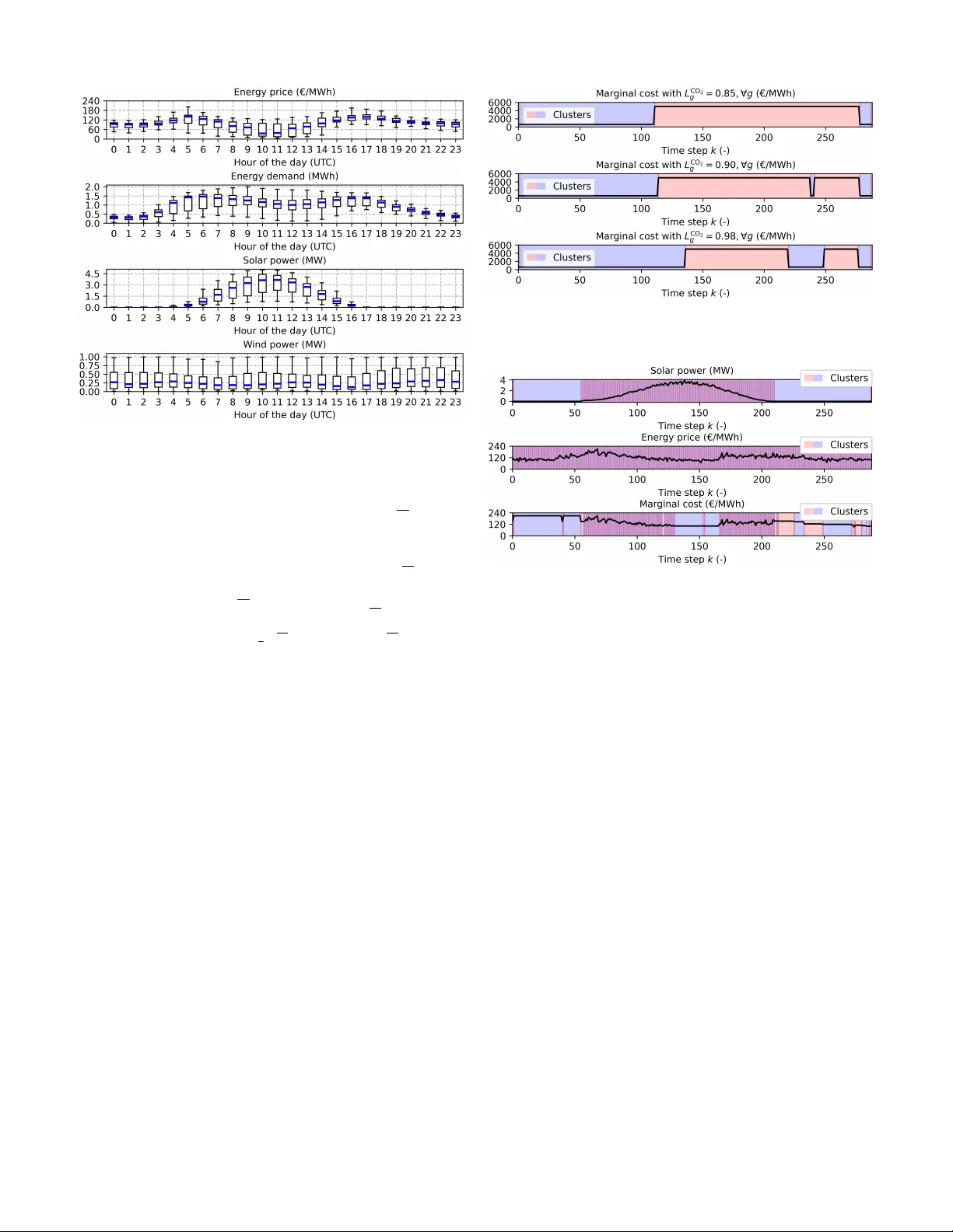
1 Stochastic V irtual Po wer Plant Dispatch via T emporally Aggre gated Distrib uted Predicti ve Control with Performance Guarantees Luca Santosuosso, Member , IEEE, Fei T eng, Senior Member , IEEE, and Sonja W ogrin, Senior Member , IEEE Abstract —This paper addresses the ener gy dispatch of a virtual power plant comprising renewable generation, energy storage, and thermal units under uncertainty in renewable output, energy prices, and energy demand. The nonlinear dynamics and multiple sources of uncertainty render traditional stochastic model predic- tive contr ol (MPC) computationally intractable as the dispatch horizon, scenario set, and asset portf olio expand. T o overcome this limitation, we propose a nov el controller that seamlessly integrates MPC with time series aggregation and distributed optimization, simultaneously r educing the temporal, asset, and scenario dimensions of the problem. The resulting contr oller pro vides a rigorous performance guarantee thr ough theoretically validated bounds on its approximation error , while leveraging dual information from pre vious MPC iterations to adaptively optimize the temporal aggregation. Numerical r esults show that the pr oposed controller r educes runtime by over 50% r elative to traditional stochastic MPC and, crucially , restores tractability where the full-scale dispatch model pr oves intractable. Index T erms —Stochastic model pr edictive contr ol, distributed model predicti ve control, time series aggregation, perf ormance guarantees, virtual power plant dispatch I . I N T R O D U C T I O N A. Literatur e Review T HE global pursuit of carbon neutrality has accelerated the widespread integration of distrib uted energy resources (DERs), including variable renewable energy sources (vRES), energy storage systems (ESSs), and flexible loads, into modern power systems. In this context, virtual po wer plants (VPPs) provide a structured framework for aggregating large popula- tions of DERs into a unified portfolio and coordinating their operation as a single entity [1], enabling efficient participation in energy trading [2] and the provision of grid services [3]. Although the potential of VPPs to enhance the flexibility of modern power systems is widely recognized [4], their operation remains a complex, multi-stage process encompass- ing long-term planning, short-term scheduling, and real-time dispatch [5]. This paper focuses on the latter stage of this decision-making process. The real-time energy dispatch of a VPP is commonly formulated as an optimal control problem [6], in which op- erations are controlled at sub-hourly resolution to optimize a performance criterion, such as minimizing generation costs, while satisfying the technical constraints of DERs. Model predictiv e control (MPC) has emerged as a widely adopted Luca Santosuosso and Sonja W ogrin are with the Institute of Elec- tricity Economics and Energy Innovation, Graz University of T echnol- ogy , and the Research Center ENERGETIC, 8010 Graz, Austria (e-mail: luca.santosuosso@tugraz.at; wogrin@tugraz.at). Fei T eng is with the Department of Electrical and Electronic En- gineering, Imperial College London, SW7 2BU London, U.K. (e-mail: f.teng@imperial.ac.uk). approach for this task, o wing to its capacity to anticipate system dynamics, explicitly enforce constraints, and iteratively update control actions based on real-time measurements [7]. As VPP operations are affected by multiple sources of uncertainty , such as energy demand, vRES generation, and market prices, pre vious research has focused on incorporating methods to handle stochasticity within MPC schemes. T radi- tional deterministic MPC assumes perfect knowledge ov er the optimization horizon [8], an assumption that is often unrealis- tic. T o address this limitation, alternativ e control schemes have been inv estigated: scenario-based stochastic MPC [9], which employs scenarios to represent potential uncertainty realiza- tions; robust MPC [10], which presumes that uncertainty is confined within a predefined set; and chance-constrained MPC [11], which enforces probabilistic guarantees on constraint sat- isfaction under stochastic variations. A comprehensive revie w of these methods is provided in [12]. Constraining uncertainty to a finite set, as in robust MPC, is often impractical for unbounded sources such as market prices and may result in e xcessively conservati ve solutions [13]. Chance-constrained MPC typically requires explicit reformu- lations to enforce probabilistic constraints, which often entail significant mathematical complexity and may also introduce conservatism. Scenario-based stochastic MPC is therefore typically preferred due to its flexibility and its ability to represent div erse uncertainty sources. Howe ver , as the size and heterogeneity of the VPP portfolio increase, the underlying uncertainty space expands accordingly , potentially requiring a prohibitiv ely large number of scenarios and rendering the MPC scheme computationally intractable. Notably , beyond increasing with the number of scenarios, i.e., the scenario dimension of the control problem, the com- putational complexity of stochastic MPC also gro ws with the number and heterogeneity of DERs within the VPP , i.e., its asset dimension [14]. Ensuring simultaneous scalability with respect to both dimensions is therefore essential to enable fast real-time dispatch of comple x, lar ge-scale VPPs [15]. T o this end, prior research has inv estigated mathematical decomposition methods for deriving distrib uted MPC schemes that partition the centralized control problem into concurrently solved subproblems, while preserving con vergence to global optimality [16]. W ithin this line of w ork, v arious distributed MPC schemes ha ve been proposed, including those based on dual decomposition [16], Douglas–Rachford splitting [17], optimality condition decomposition (OCD) [18], analytical target cascading (A TC) [10], approximate Newton direction methods [19], and the widely used alternating direction method of multipliers (ADMM) [20]. Among these, ADMM and its variants [21] have gained widespread adoption due to their 2 flexibility in handling di verse problem formulations and their well-established con vergence properties [22]. Notably , while sev eral studies have distrib uted computations across either the scenario [23] or the asset [24] dimension of VPP optimization models independently , few ha ve addressed both simultaneously [25]. Crucially , none of these studies addresses scalability across the third complexity dimension of the problem, namely its temporal dimension , thereby leaving substantial potential for reducing the computational b urden of MPC schemes unexploited. This occurs because temporal decomposition decouples the intertemporal constraints of the original model, producing subproblems that are inherently more challenging to coordinate to ward con ver gence than those resulting from decompositions across assets or scenarios [18]. T o alle viate the computational burden associated with the temporal dimension of ener gy optimization models, time series aggregation (TSA) methods ha ve emerged as a highly ef fectiv e alternativ e to decomposition methods. By compacting the full- scale optimization model, TSA produces an aggregated model defined ov er a reduced set of representati ve time periods (or clusters), while aiming to preserv e the essential temporal dy- namics of the original formulation [26]. Unlike decomposition methods, which aim at reducing computational comple xity via parallelization, TSA seeks the same objectiv e through a dimensionality reduction of the original optimization model. T raditional a priori TSA methods typically employ stan- dard clustering techniques, such as k-means [27], k-medoids [28], and hierarchical clustering [29], to construct temporally aggregated models based solely on the statistical features of the input time series. More recently , a posteriori TSA has emerged as an alternativ e paradigm, augmenting the clustering procedure with features deri ved from the optimization model itself, such as insights from pre vious optimization runs, to yield aggregations that more accurately capture the temporal dynamics of the original full-scale optimization model [30]. Remarkably , a posteriori TSA has the potential to achie ve exact temporal aggreg ation [31], yielding an aggregated model that faithfully replicates the output of its full-scale counterpart while deliv ering substantial computational sa vings. While many studies have proposed TSA methods for large- scale energy optimization models [32], particularly for those in volving intertemporal constraints that complicate the TSA procedure by requiring the preservation of temporal chronol- ogy [33], research on integrating TSA within MPC schemes remains scarce [34]. Notably , none of the existing studies in- vestigates the potential of emerging a posteriori TSA methods to reduce the temporal dimension in stochastic MPC. Furthermore, since TSA yields an aggregated model that approximates its full-scale counterpart, it is essential in prac- tical applications to provide performance guarantees by quan- tifying the approximation error introduced through temporal aggregation. While formal guarantees have been established for linear programming (LP) [35], mixed-inte ger linear (MILP) and mixed-inte ger quadratic programming (MIQP) problems [36], these theoretical results are not readily e xtendable to quadratic programming (QP) and quadratically constrained quadratic programming (QCQP) formulations, which are com- monly employed in the ener gy dispatch of VPPs [5]. B. Resear ch Gaps and Contributions The literature revie w re veals the following research gaps: • Prior studies sho w that decomposition methods ef fec- tiv ely enhance the scalability of energy dispatch problems along the scenario and asset dimensions [10], [16]–[20], while TSA, particularly a posteriori TSA, has pro ven effecti ve in reducing the temporal dimension without compromising solution accuracy [27]–[31]. Ho wev er , the systematic integration of these two complementary methodologies within MPC schemes remains largely un- explored, lea ving significant potential for further reducing the computational complexity of real-time controllers. • Existing research on performance guarantees for TSA methods has primarily focused on establishing bounds on the approximation error incurred by aggre gated optimiza- tion models relati ve to their full-scale counterparts. T o date, such guarantees ha ve been deriv ed only for LP [35], MILP , and MIQP problems [36], typically by constructing aggregated models in which the decision variables are av- eraged ov er the representativ e time periods. Howe ver , for QCQP problems commonly encountered in VPP dispatch [5], the simultaneous presence of quadratic constraints, time-varying parameters, and intertemporal constraints (e.g., due to storage and ramping) renders this averaging approach insufficient: as discussed in Section II, the previously established bounds no longer hold. This paper seeks to address these research gaps through the following key contrib utions : • W e formulate the energy dispatch of a VPP as a QCQP problem and propose a stochastic MPC scheme for its real-time solution. The stochastic MPC scheme is decom- posed along both its asset and scenario dimensions using consensus ADMM, and temporally aggreg ated via TSA. This integrated approach, featuring a nov el combination of MPC, TSA, and distributed optimization, simultane- ously addresses all complexity dimensions of the dispatch problem, thereby maximizing computational ef ficiency . • W e demonstrate that the deriv ed controller always pro- vides a lower bound on the optimal objective function value of its full-scale counterpart, e ven in the presence of quadratic constraints, time-varying parameters, and intertemporal constraints such as storage and ramping. • Leveraging the solution of the temporally aggregated and distributed controller , we propose an algorithm to system- atically compute an upper bound on the optimal objecti ve function value of the full-scale dispatch problem. The gap between the upper and lower bounds quantifies the approximation error incurred at each MPC iteration, thereby providing a rigorous performance guarantee. • Although the derived bounds hold independently of the clustering technique employed for TSA, we show that incorporating dual information from the dispatch model into the clustering features yields a temporally aggregated controller that exactly reproduces the full-scale solution. Since such dual information is not av ailable ex ante , we propose a closed-loop, a posteriori TSA method lev eraging past MPC iterations to estimate it. 3 T ABLE I C O MPA R IS O N O F T H IS S T UD Y W I TH T H E R E L EV A N T R E L A T E D L I TE R A T U R E Ref. MPC Problem Decomposition Distributed method TSA Perf ormance-guaranteed [9] ✓ (stochastic) QP × − × ✓ [11] ✓ (chance-constrained) QP × − × ✓ [16] ✓ (deterministic) QP Asset Dual decomposition × ✓ [10] ✓ (robust) MILP Asset A TC × × [20] ✓ (stochastic) MIQP Asset ADMM × × [18] ✓ (stochastic) QP Scenario & temporal OCD × ✓ [29] × LP × − ✓ (a priori) × [30] × MILP × − ✓ (a posteriori) × [35] × LP × − ✓ (a priori) ✓ [36] × MILP & MIQP × − ✓ (a priori) ✓ [34] ✓ (deterministic) MIQP × − ✓ (a priori) × This paper ✓ (stochastic) QCQP Asset & scenario ADMM ✓ (a posteriori) ✓ T able I compares this study with the rele vant related literature. The remainder of the paper is org anized as follows: Sec- tion II details the proposed methodology , Section III presents the results, and Section IV concludes the study . I I . M E T H O D O L O G Y In the follo wing, sets and vectors are denoted in boldface (e.g., z ). The cardinality of a set is denoted by | · | , while ∥ · ∥ 2 denotes the Euclidean ( ℓ 2 ) norm. The maximum and minimum elements of a set Φ are denoted by max( Φ ) and min( Φ ) , respectiv ely . The zero vector is denoted by 0 . All sets are indexed starting from 0 . A. Overview of the Pr oposed Methodolo gy In this section, we present the proposed methodology for real-time VPP dispatch under uncertainty . The VPP comprises vRES, namely wind and solar , a set of energy storage systems N indexed by n , and a set of thermal power plants G indexed by g . The dispatch problem is subject to various uncertainties, namely vRES generation, ener gy demand, and energy prices, captured by a set of scenarios Ω index ed by ω . While vRES are non-dispatchable, storage and thermal units can be dispatched to maximize profit while meeting the VPP internal demand, with any imbalances accommodated via non-supplied energy . The VPP modeling is detailed in Subsection II-B. The dispatch problem is addressed using a stochastic MPC scheme, as discussed in Subsection II-C. At each time step t ∈ T , the MPC scheme is solv ed over a prediction horizon K , indexed by k , with cardinality K : = | K | and sampling time ∆ . F ollowing the standard MPC paradigm, at each time step t , only the first control action (corresponding to k = 0 ) is applied, after which the horizon is advanced by one time step. T o streamline the notation, we use the subscript k to denote variables and parameters associated with time t + k , i.e., the k -th prediction step of the MPC iteration executed at time t . Our goal is to optimize the real-time ener gy dispatch of a VPP while simultaneously reducing the computational com- plexity of the problem across its asset, scenario, and temporal dimensions. T o achieve this, we propose a nov el integration of MPC, a posteriori TSA, and distributed optimization. Fig. 1 presents an overvie w of the proposed methodology . The a posteriori TSA module exploits dual information from the previous MPC iteration to aggregate the full-scale controller across R representative time periods, indexed by r . The resulting temporally aggregated controller is then simulta- neously decomposed across assets and scenarios, yielding the proposed temporally aggregated and distrib uted stochastic MPC scheme , as detailed in Subsection II-F. The temporally aggregated stochastic MPC scheme and a posteriori TSA method are detailed in Subsections II-D and II-E, respectiv ely . As illustrated in Fig. 1, the controller deliv ers a rigorous performance guarantee via iterati vely refined upper and lower bounds on the full-scale optimal objectiv e function value. The gap between these bounds enables the decision- maker to assess the controller performance without requiring the full-scale model solution, as discussed in Subsection II-G. B. Modeling The VPP dispatch is modeled as follows. For each scenario ω and time step k , the forecasts of vRES generation, demand, and energy prices are denoted by P vRES ω ,k , D ω ,k , and π ω ,k , respectiv ely . The energy output of the VPP in scenario ω at time k is denoted by e ω ,k , while e ns ω ,k is the non-supplied energy demand. For each storage unit n , the state of charge at time k in scenario ω is denoted by e s n,ω ,k , with char ging and discharging po wers denoted by p c n,ω ,k and p d n,ω ,k , respectively . The minimum and maximum char ging (discharging) power limits are denoted by P c n and P c n ( P d n and P d n ). Charging and discharging efficiencies are denoted by η c n and η d n . The initial state of char ge is E s , 0 n , while the lower and upper bounds on the state of char ge are E s n and E s n , respectiv ely . The dynamics of each energy storage system are gi ven by e s n,ω ,k +1 = e s n,ω ,k +  η c n p c n,ω ,k − η d n p d n,ω ,k  ∆ , ∀ n, ∀ ω , ∀ k ∈ K \ { K − 1 } , (1) e s n,ω , 0 = E s , 0 n , ∀ n, ∀ ω , (2) E s n ≤ e s n,ω ,k ≤ E s n , ∀ n, ∀ ω , ∀ k . (3) The charging and discharging powers are constrained by P c n ≤ p c n,ω ,k ≤ P c n , ∀ n, ∀ ω , ∀ k , (4) P d n ≤ p d n,ω ,k ≤ P d n , ∀ n, ∀ ω , ∀ k . (5) The power output of each thermal unit g , denoted p th g ,ω ,k , is constrained between its lower ( P th g ) and upper ( P th g ) limits as P th g ≤ p th g ,ω ,k ≤ P th g , ∀ g , ∀ ω , ∀ k . (6) 4 Fig. 1. Illustration of the proposed methodology for real-time energy dispatch of a VPP under uncertainty . Moreov er, the thermal power generation of the VPP is subject to the following quadratic emission constraints [37]: α g  p th g ,ω ,k  2 + β g p th g ,ω ,k ≤ L CO 2 g , ∀ g , ∀ ω , ∀ k , (7) where L CO 2 g is the emission limit of generator g , while α g and β g are the coefficients mapping its output to emissions. Each thermal unit is subject to its ramp limit R th g as p th g ,ω ,k +1 − p th g ,ω ,k ≤ R th g , ∀ g , ∀ ω , ∀ k ∈ K \ { K − 1 } , (8) p th g ,ω ,k − p th g ,ω ,k +1 ≤ R th g , ∀ g , ∀ ω , ∀ k ∈ K \ { K − 1 } . (9) C. Full-Scale Controller W e formulate the VPP energy dispatch as a stochastic MPC problem. Let u 0 denote the vector of control actions computed for k = 0 . W e define the set of decision variables as z : =  u 0 , e ω ,k , e ns ω ,k , e s n,ω ,k , p th g ,ω ,k , p c n,ω ,k , p d n,ω ,k  n ∈ N ,g ∈ G ,ω ∈ Ω ,k ∈ K . Let C c n and C d n denote the char ging and discharging costs of storage unit n , respectively , and let C th g represent the generation cost of thermal unit g . The penalty associated with non-supplied energy is denoted by C ns . Furthermore, a reference state E ref n is specified for each storage unit n ; deviations from this reference are penalized by C ref n . The goal is to minimize the objective function F ( z ) : = X ω ∈ Ω X k ∈ K  − π ω ,k e ω ,k + X g ∈ G C th g p th g ,ω ,k ∆ + C ns e ns ω ,k + X n ∈ N  C c n p c n,ω ,k + C d n p d n,ω ,k  ∆  + X n ∈ N X ω ∈ Ω X k ∈ K C ref n  e s n,ω ,k − E ref n  2 . (10) In (10), linear terms capture the VPP profit, while the quadratic term penalizes storage de viations from the reference states. At each time t ∈ T , the full-scale stochastic MPC scheme solves the follo wing QCQP problem over the horizon K : min z F ( z ) (11a) s.t. e ω ,k = P vRES ω ,k ∆ − D ω ,k + X n ∈ N  p d n,ω ,k − p c n,ω ,k  ∆ + X g ∈ G p th g ,ω ,k ∆ + e ns ω ,k , ∀ ω , ∀ k , (11b) (1) − (9) ,  e ns ω , 0 , p th g ,ω , 0 , p c n,ω , 0 , p d n,ω , 0  = u 0 , ∀ n, ∀ g , ∀ ω , (11c) z ≥ 0 . (11d) In (11), the constraints (11b) enforce the ener gy balance within the VPP , while (11c) are the non-anticipativity constraints. D. T emporally Aggr egated Contr oller T o alle viate computational burden, we employ TSA to construct a temporally aggregated counterpart of (11), defined ov er R representativ e time periods, with R : = | R | . When R ≪ K , solving the aggregated model in place of its full-scale counterpart yields a significant computational advantage. Let K r ⊆ K denote the set of time periods assigned to cluster r ∈ R , with cardinality K r : = | K r | . W e collect the decision variables of the aggregated model in ¯ z : = { ¯ u 0 , ¯ e ω ,r , ¯ e ns ω ,r , ¯ e s n,ω ,r , ¯ p th g ,ω ,r , ¯ p c n,ω ,r , ¯ p d n,ω ,r } n ∈ N ,g ∈ G ,ω ∈ Ω ,r ∈ R . W e define the aggre gated counterpart of F ( z ) in (10) as ¯ F ( ¯ z ) : = X ω ∈ Ω X r ∈ R K r  − max k ∈ K r { π ω ,k } ¯ e ω ,r + X g ∈ G C th g ¯ p th g ,ω ,r ∆ + C ns ¯ e ns ω ,r + X n ∈ N  C c n ¯ p c n,ω ,r + C d n ¯ p d n,ω ,r  ∆  + X n ∈ N X ω ∈ Ω X r ∈ R C ref n  ¯ e s n,ω ,r − E ref n  2 . (12) At each time t ∈ T , the temporally aggregated stochastic MPC scheme solves the following QCQP problem ov er R : min ¯ z ¯ F ( ¯ z ) (13a) s.t. ¯ e ω ,r = X k ∈ K r P vRES ω ,k ∆ − D ω ,k K r + X g ∈ G ¯ p th g ,ω ,r ∆ + ¯ e ns ω ,r + X n ∈ N  ¯ p d n,ω ,r − ¯ p c n,ω ,r  ∆ , ∀ ω , ∀ r, (13b) ¯ e s n,ω ,r +1 = ¯ e s n,ω ,r + K r  η c n ¯ p c n,ω ,r − η d n ¯ p d n,ω ,r  ∆ , ∀ n, ∀ ω , ∀ r ∈ R \ { R − 1 } , (13c) ¯ e s n,ω , 0 = E s , 0 n , ∀ n, ∀ ω , (13d) 5 E s n ≤ ¯ e s n,ω ,r ≤ E s n , ∀ n, ∀ ω , ∀ r, (13e) P c n ≤ ¯ p c n,ω ,r ≤ P c n , ∀ n, ∀ ω , ∀ r, (13f) P d n ≤ ¯ p d n,ω ,r ≤ P d n , ∀ n, ∀ ω , ∀ r, (13g) P th g ≤ ¯ p th g ,ω ,r ≤ P th g , ∀ g , ∀ ω , ∀ r , (13h) α g K r  ¯ p th g ,ω ,r  2 − α g ( K r − 1)  P th g  2 + β g ¯ p th g ,ω ,r ≤ L CO 2 g , ∀ g , ∀ ω , ∀ r , (13i) ¯ p th g ,ω ,r +1 − ¯ p th g ,ω ,r K r ≤ R th g + R th g K r +1 − 1 2 , ∀ g , ∀ ω , ∀ r ∈ R \ { R − 1 } , (13j) ¯ p th g ,ω ,r − ¯ p th g ,ω ,r +1 K r +1 ≤ R th g + R th g K r − 1 2 , ∀ g , ∀ ω , ∀ r ∈ R \ { R − 1 } , (13k)  ¯ e ns ω , 0 , ¯ p th g ,ω , 0 , ¯ p c n,ω , 0 , ¯ p d n,ω , 0  = ¯ u 0 , ∀ n, ∀ g , ∀ ω , (13l) ¯ z ≥ 0 . (13m) Here, (13b), (13c)–(13k), (13l), and (13m) are the aggregated counterparts of (11b), (1)–(9), (11c), and (11d), respecti vely . Notably , whereas con ventional TSA methods average the input time series over each cluster [26], we introduce a novel formulation that instead considers the cluster-wise maximum price in (12) and augments the quadratic constraints (13i) and the intertemporal constraints (13c), (13j), and (13k) with cluster-specific terms. This ensures that the temporally aggre- gated model (13) inherently satisfies the desired theoretical properties, as formally established in Subsection II-G. E. Closed-Loop A P osteriori T ime Series Ag gre gation Once the temporally aggregated model (13) is constructed, a clustering technique is required to extract representati ve time periods from the original prediction horizon K . Owing to the presence of intertemporal constraints in (11), conv entional clustering techniques (e.g., k-means) cannot be directly em- ployed, as they disregard temporal chronology . T o address this issue, we employ a sliding window clustering technique. Let { a k } k ∈ K be the set of clustering features used for TSA. This technique ev aluates the similarity between consecutiv e elements of { a k } , assigning k to the current cluster r if ∥ a k − µ r ∥ 2 ≤ ζ , (14) where ζ is a user-defined similarity threshold and µ r denotes the centroid of cluster r , computed as µ r : = 1 K r P k ∈ K r a k . If condition (14) is not satisfied for a k , the current cluster is closed and a ne w cluster is initialized starting at k . Fig. 2 illustrates the sliding windo w clustering technique. Starting from an initial cluster (e.g., containing k − 1 and k ), the cluster is extended to include k + 1 only if condition (14) is satisfied for a k +1 , thereby ensuring temporal coherence. The features used for TSA directly affect the fidelity of the aggre gated model. In particular , [31] demonstrates that if the active constraints of the full-scale model were known, an aggregated model could be constructed that exactly reproduces the optimal objective function v alue of the full-scale model. Although such information is unav ailable ex ante , MPC offers a unique opportunity to exploit it retrospecti vely , as Fig. 2. Illustration of the sliding window clustering technique. the same optimization problem is repeatedly solved o ver ov erlapping horizons, differing only by the newly appended terminal time step and the set of scenarios considered at each MPC iteration. Consequently , the outputs from previous MPC runs can inform TSA in a closed-loop manner . Motiv ated by this insight, we propose a closed-loop a poste- riori TSA method integrated with MPC. At each iteration t , the dual information from the MPC problem solved at time t − 1 is used as a feature in the sliding window clustering technique to identify the representativ e periods R (see Fig. 1). Specifically , we use estimates of the marginal costs, i.e., the dual variables associated with the energy balance constraints (11b), which, as shown in Section III, serve as an accurate proxy for identifying the acti ve constraints of (11). T wo singleton clusters are enforced at the first and last time steps of K , reflecting the absence of dual information at the terminal step and the critical role of the initial step, whose control actions are implemented at time t . By exploiting dual information from the previous MPC iteration, our method estimates the activ e constraints of (11), directly tar geting exact temporal aggreg ation, which is typically unattainable with traditional a priori TSA methods. F . T emporally Aggr egated and Distrib uted Contr oller T o further reduce the computational complexity arising from the asset and scenario dimensions, we decompose the temporally aggregated model (13) via consensus ADMM [21]. The aggregated model (13) features three sets of coupling constraints: intertemporal coupling induced by the storage (13c) and ramping constraints (13j)–(13k), asset coupling arising from the energy balance constraints (13b), and sce- nario coupling induced by the non-anticipativity constraints (13l). All coupling constraints in (13) inv olve three sets of global variables : ¯ p c n,ω : =  ¯ p c n,ω , 0 , ..., ¯ p c n,ω ,r , ..., ¯ p c n,ω ,R − 1  ⊤ , ¯ p d n,ω : =  ¯ p d n,ω , 0 , ..., ¯ p d n,ω ,r , ..., ¯ p d n,ω ,R − 1  ⊤ , and ¯ p th g ,ω : =  ¯ p th g ,ω , 0 , ..., ¯ p th g ,ω ,r , ..., ¯ p th g ,ω ,R − 1  ⊤ . W e relax the coupling con- straints in (13) by introducing copies of these global variables. Let  ˆ p c n,ω , ˆ p d n,ω , ˆ p th g,ω  and  ˜ p c n,ω , ˜ p d n,ω , ˜ p th g,ω  denote two distinct sets of copies of the global v ariables in (13). By intro- ducing these copies, we reformulate the temporally aggregated model (13) as the follo wing consensus problem: min ¯ z ¯ F ( ¯ z ) (15a) s.t. z b ∈ Ξ ( β ) , (15b) z s n,ω ∈ Γ s n,ω  θ s n,ω  , ∀ n, ∀ ω , (15c) ˜ p th g ,ω ∈ Γ th g ,ω  θ th g ,ω  , ∀ g , ∀ ω , (15d) 6 ¯ p s n,ω = ˆ p s n,ω : ˆ λ s n,ω , ∀ n, ∀ ω , (15e) ¯ p s n,ω = ˜ p s n,ω : ˜ λ s n,ω , ∀ n, ∀ ω , (15f) ¯ p th g ,ω = ˆ p th g ,ω : ˆ λ th g ,ω , ∀ g , ∀ ω , (15g) ¯ p th g ,ω = ˜ p th g ,ω : ˜ λ th g ,ω , ∀ g , ∀ ω , (15h) where ˆ λ s n,ω : = h ˆ λ c n,ω , ˆ λ d n,ω i ⊤ , ˜ λ s n,ω : = h ˜ λ c n,ω , ˜ λ d n,ω i ⊤ , ˜ p s n,ω : = [ ˜ p c n,ω , ˜ p d n,ω ] ⊤ , ˆ p s n,ω : = [ ˆ p c n,ω , ˆ p d n,ω ] ⊤ , ¯ p s n,ω : = [ ¯ p c n,ω , ¯ p d n,ω ] ⊤ , z b : =  ¯ u 0 , ¯ e ω ,r , ¯ e ns ω ,r , ˆ p c n,ω , ˆ p d n,ω , ˆ p th g ,ω  n ∈ N ,g ∈ G ,ω ∈ Ω ,r ∈ R , and z s n,ω : =  ¯ e s n,ω , ˜ p c n,ω , ˜ p d n,ω  . This reformulation introduces three sets of temporally ag- gregated subproblems: • Subproblem (16), corresponding to (15b), with local variables z b , and feasible set Ξ ( β ) , defined by (13b), (13f)–(13h), (13l) and (13m), with parameters β . • | N | × | Ω | subproblems (17), corresponding to (15c), with local v ariables z s n,ω , and feasible set Γ s n,ω  θ s n,ω  , defined by (13c)–(13g) and (13m), with parameters θ s n,ω . • | G | × | Ω | subproblems (18), corresponding to (15d), with local variables ˜ p th g ,ω and feasible set Γ th g ,ω ( θ th g ,ω ) defined by (13h)–(13k) and (13m), with parameters θ th g ,ω . Consistency among the local variables is enforced by the con- sensus constraints (15e)–(15h), with associated dual variables ˆ λ s n,ω , ˜ λ s n,ω , ˆ λ th g ,ω , and ˜ λ th g ,ω . Separately for each scenario, the subproblems (17) and (18) determine the dispatch of each storage and thermal unit, respectiv ely , while (16) enforces the VPP energy balance. The deriv ed ( | N | + | G | ) × | Ω | + 1 subproblems are solved in parallel via consensus ADMM. Let ρ be ADMM step size. At time t , our temporally ag- gregated and distributed stochastic MPC scheme executes the following steps over i ∈ I iterations, with I : = | I | . Step I . Local primal variable update: z b i +1 : = argmin z b ∈ Ξ ( X ω ∈ Ω X r ∈ R K r  C ns ¯ e ns ω ,r − max k ∈ K r { π ω ,k } ¯ e ω ,r  + X n ∈ N X ω ∈ Ω  ˆ λ s i n,ω  ⊤ ˆ p s n,ω + ρ 2    ˆ p s n,ω − ¯ p s i n,ω    2 2 ! + X g ∈ G X ω ∈ Ω  ˆ λ th i g ,ω  ⊤ ˆ p th g ,ω + ρ 2    ˆ p th g ,ω − ¯ p th i g ,ω    2 2 ! ) , (16) z s i +1 n,ω : = argmin z s n,ω ∈ Γ s n,ω ( X n ∈ N X ω ∈ Ω X r ∈ R  C c n ˜ p c n,ω ,r + C d n ˜ p d n,ω ,r  K r ∆ + X n ∈ N X ω ∈ Ω X r ∈ R C ref n  ¯ e s n,ω ,r − E ref n  2 +  ˜ λ s i n,ω  ⊤ ˜ p s n,ω ! + X n ∈ N X ω ∈ Ω  ρ 2    ˜ p s n,ω − ¯ p s i n,ω    2 2  ) , ∀ n, ∀ ω , (17) ˜ p th i +1 g ,ω : = argmin ˜ p th g,ω ∈ Γ th g,ω ( X g ∈ G X ω ∈ Ω X r ∈ R C th g ˜ p th g ,ω ,r K r ∆ +  ˜ λ th i g ,ω  ⊤ ˜ p th g ,ω ! + X g ∈ G X ω ∈ Ω  ρ 2    ˜ p th g ,ω − ¯ p th i g ,ω    2 2  ) , ∀ g , ∀ ω . (18) Step II . Global primal variable update: ¯ p s i +1 n,ω : = 1 2  ˆ p s i +1 n,ω + ˜ p s i +1 n,ω  , ∀ n, ∀ ω , (19) ¯ p th i +1 g ,ω : = 1 2  ˆ p th i +1 g ,ω + ˜ p th i +1 g ,ω  , ∀ g , ∀ ω . (20) Step III . Dual variable update: ˆ λ s i +1 n,ω : = ˆ λ s i n,ω + ρ  ˆ p s i +1 n,ω − ¯ p s i +1 n,ω  , ∀ n, ∀ ω , (21) ˜ λ s i +1 n,ω : = ˜ λ s i n,ω + ρ  ˜ p s i +1 n,ω − ¯ p s i +1 n,ω  , ∀ n, ∀ ω , (22) ˆ λ th i +1 g ,ω : = ˆ λ th i g ,ω + ρ  ˆ p th i +1 g ,ω − ¯ p th i +1 g ,ω  , ∀ g , ∀ ω , (23) ˜ λ th i +1 g ,ω : = ˜ λ th i g ,ω + ρ  ˜ p th i +1 g ,ω − ¯ p th i +1 g ,ω  , ∀ g , ∀ ω . (24) T o enhance conv ergence, we adopt the residual-based update rule for ρ , initialized at ρ 0 , as proposed in [21]. G. Derivation of the Objective Function Bounds In Subsection II-F, the aggregated model (13) is decom- posed using ADMM. Since (13) is con vex, ADMM is guaran- teed to con verge to its optimal objecti ve function value [21]. Howe ver , (13) is an approximation of the original full-scale model (11). T o establish a formal performance guarantee, we bound the resulting approximation error as follows. Proposition 1. Let z be a feasible solution to the full-scale model (11) . Let ¯ z be derived fr om z as ¯ e ω ,r : = X k ∈ K r e ω ,k K r , (25) ¯ e ns ω ,r : = X k ∈ K r e ns ω ,k K r , (26) ¯ e s n,ω ,r : = e s n,ω , min( K r ) , (27) ¯ p th g ,ω ,r : = X k ∈ K r p th g ,ω ,k K r , (28) ¯ p c n,ω ,r : = X k ∈ K r p c n,ω ,k K r , (29) ¯ p d n,ω ,r : = X k ∈ K r p d n,ω ,k K r , (30) ∀ n, ∀ g , ∀ ω , ∀ r . Then, ¯ z is a feasible solution to the tempo- rally aggr e gated model (13) and it holds that ¯ F ( ¯ z ) ≤ F ( z ) . Pr oof. W e first demonstrate that any ¯ z obtained through (25)– (30) is feasible for the temporally aggregated model (13). Using (30), we reformulate (13j) and (13k) as ¯ p th g ,ω ,r +1 − ¯ p th g ,ω ,r K r = X k ∈ K r +1 p th g ,ω ,k K r +1 − X k ∈ K r p th g ,ω ,k ≤ p th g ,ω , min( K r +1 ) + R th g K r +1 − 1 2 − p th g ,ω , max( K r ) ≤ R th g + R th g K r +1 − 1 2 , ∀ g , ∀ ω , ∀ r ∈ R \ { R − 1 } , (31) and ¯ p th g ,ω ,r − ¯ p th g ,ω ,r +1 K r +1 = X k ∈ K r p th g ,ω ,k K r − X k ∈ K r +1 p th g ,ω ,k ≤ p th g ,ω , max( K r ) + R th g K r − 1 2 − p th g ,ω , min( K r +1 ) ≤ R th g + R th g K r − 1 2 , ∀ g , ∀ ω , ∀ r ∈ R \ { R − 1 } , (32) 7 respectiv ely . Using (28), we reformulate (13i) as α g K r X k ∈ K r p th g ,ω ,k ! 2 − α g ( K r − 1)  P th g  2 + β g K r X k ∈ K r p th g ,ω ,k ≤ X k ∈ K r α g  p th g ,ω ,k  2 + β g p th g ,ω ,k K r ≤ L CO 2 g , ∀ g , ∀ ω , ∀ r . (33) The full-scale constraints (8), (9), and (7) imply the aggre- gated constraints (31), (32), and (33), respecti vely , since they are enforced ov er the set K r rather than ov er the individual time steps k . Similarly , constraints (11b), (1)–(6), and (11c) imply (13b)–(13h) and (13l), as demonstrated in [36]. It follows that an y ¯ z obtained from a feasible solution z of the full-scale model (11) via (25)–(30) is feasible for (13). Finally , substituting ¯ z into ¯ F ( ¯ z ) , as defined in (12), yields X ω ∈ Ω X r ∈ R − max k ∈ K r { π ω ,k } X k ∈ K r e ω ,k ! + X ω ∈ Ω X k ∈ K C ns e ns ω ,k + X ω ∈ Ω X k ∈ K   X g ∈ G C th g p th g ,ω ,k + X n ∈ N  C c n p c n,ω ,k + C d n p d n,ω ,k    ∆ + X n ∈ N X ω ∈ Ω X r ∈ R C ref n  e s n,ω , min( K r ) − E ref n  2 ≤ F ( z ) , where F ( z ) is defined as in (10). In words, Proposition 1 asserts that e very feasible solution of the full-scale model (11) corresponds to a feasible solution of the temporally aggregated model (13) with an equal or lo wer objectiv e function value. Consequently , the controller proposed in Subsection II-F pro vides a guaranteed lo wer bound on the optimal objectiv e function v alue of the original full-scale controller in Subsection II-C at each MPC iteration. Once a lo wer bound F LB on the full-scale optimal objective function value F ⋆ is obtained, as established in Proposition 1, an upper bound F UB is computed by solving (11) with the first-stage decisions u 0 fixed to those obtained from solving (13). Under this restriction, (11) can be solv ed in paral- lel across scenarios. The resulting performance-guaranteed temporally aggr egated and distrib uted stochastic MPC scheme executes Algorithm 1 at each time step t ∈ T . Algorithm 1 is structured into a higher and a lower layer , ex ecuting j ∈ J and i ∈ I iterations, respectiv ely . At time t , the higher layer receiv es the dual v ariable v alues computed at time t − 1 , specifically the marginal cost estimates, which serve as features for the sliding windo w clustering technique detailed in Subsection II-E. The identified clusters are then used to construct the temporally aggregated model (13), which is passed to the lower layer . Here, the problem is decomposed into ( | N | + | G | ) × | Ω | + 1 temporally aggreg ated subproblems, which are solved in parallel across assets and scenarios via consensus ADMM. Upon con vergence of ADMM, determined according to the residual-based terminal condition of [21], the solution of the aggregated model is emplo yed to compute F UB and F LB . If the relativ e difference between these bounds falls below the threshold ϵ thr , the algorithm terminates; otherwise ζ , Algorithm 1 Performance-Guaranteed Distributed Stochastic Predictiv e Control with A Posteriori Time Series Aggregation Input: β , n θ s n,ω , θ th g ,ω o n ∈ N ,g ∈ G ,ω ∈ Ω , γ , ρ 0 , ϵ thr , ζ 0 , J , I . Output: Bounds F UB ⋆ and F LB ⋆ , and control actions ¯ u ⋆ 0 . 1: j ← 0 , ζ j ← ζ 0 ; 2: Higher layer - T emporal aggr e gation : 3: while 100    F UB j +1 − F LB j +1 F UB j +1    > ϵ thr and j < J do 4: Perform TSA as detailed in Subsection II-E, using ζ j and the average marginal costs across scenarios from the previous MPC iteration as features; 5: i ← 0 , ρ ← ρ 0 , n ¯ p s 0 n,ω ← 0 2 R , ¯ p th 0 g ,ω ← 0 R , ˆ λ s 0 n,ω ← 0 2 R , ˜ λ s 0 n,ω ← 0 2 R , ˆ λ th 0 g ,ω ← 0 R , ˜ λ th 0 g ,ω ← 0 R , ∀ n, ∀ g , ∀ ω o ; 6: Lower layer - Consensus ADMM : 7: while the residual-based terminal condition from [21] is not satisfied and i < I do 8: n z b i +1 , z s i +1 n,ω , ˜ p th i +1 g ,ω o ← Solve (16)–(18); 9: n ¯ p s i +1 n,ω , ¯ p th i +1 g ,ω o ← Solve (19)–(20); 10:  ˆ λ s i +1 n,ω , ˜ λ s i +1 n,ω , ˆ λ th i +1 g ,ω , ˜ λ th i +1 g ,ω  ← Solve (21)–(24); 11: Residual-based adaptiv e update of ρ from [21]; 12: i ← i + 1 ; 13: end while 14: ¯ u ⋆ 0 ← Solve (13l), and ¯ F ⋆ ← Solve (12); 15: F PRJ ← Solve the full-scale stochastic model (11) with u 0 = ¯ u ⋆ 0 ; ▷ In parallel ∀ ω 16: F LB j +1 ← ¯ F ⋆ , and F UB j +1 ← min  F UB j , F PRJ  ; 17: ζ j +1 ← γ ζ j ; 18: j ← j + 1 ; 19: end while 20: return F UB ⋆ ← F UB j , F LB ⋆ ← F LB j and ¯ u ⋆ 0 ; initialized to ζ 0 , is reduced by a positiv e factor γ < 1 , and the algorithm iterates again. Being the result of a projection step, the control actions computed by Algorithm 1 at time t , denoted by ¯ u ⋆ 0 , are feasible for the full-scale model (11). As illustrated in Fig. 1, Algorithm 1 provides a formal performance guar - antee by allowing the decision-maker to ev aluate the achiev ed optimality gap (i.e., the relativ e difference between upper and lower bounds) at each iteration. I I I . S I M U L A T I O N R E S U LT S A N D D I S C U S S I O N This section presents the case study (Subsection III-A) and discusses the numerical results (Subsections III-B and III-C). A. Case Study Description W e simulate the VPP energy dispatch ov er one year using a prediction horizon of 24 h and a sampling time of ∆ = 5 min, i.e., | K | = 288 . T o ensure transparency and reproducibility , the VPP parameters are sampled from prescribed distributions. For each storage unit, the minimum state of charge and charging/dischar ging power are set to 0 MWh and 0 MW , re- spectiv ely . The energy capacity is drawn from a uniform distri- bution over [1 , 5] MWh, while maximum charging/discharging 8 Fig. 3. Boxplots of the hourly uncertainty realization values. The box represents the interquartile range, the blue line indicates the median, and the whiskers extend to the minimum and maximum observations. power limits are drawn uniformly from [0 . 1 MW , E s n / (1 h)] . The initial state is set to 0 MWh, and char ging and dis- charging efficiencies are sampled uniformly from [0 . 7 , 0 . 9] and [1 / 0 . 9 , 1 / 0 . 7] , respectively . The reference states are E s n / 2 , ∀ n . For each thermal unit, P th g = 0 MW , the capacity is drawn uniformly from [0 , 2] MW , the ramp limit is P th g / 6 , and the parameters in (7) are α g = 1 2  P th g  − 2 , β g =  2 P th g  − 1 , and L CO 2 g = 0 . 9 . Thermal and storage operation costs are drawn uniformly from [30 , 60] and [5 , 15] e /MWh, respectiv ely . The cost of non-supplied energy is 5000 e /MWh, and deviations from storage reference states incur a cost of 1 e /(MWh) 2 . The uncertainty realizations are represented by scaled day- ahead ener gy prices, ener gy demand, and wind and solar power generation in Austria for 2024, obtained from the ENTSO-E T ransparency Platform [38] and illustrated in Fig. 3. Scenarios are generated by perturbing these observations with Laplace- distributed noise L ( µ, b k ) , where the scale parameter is set to b k = 0 . 1 k for k ∈ K , reflecting the progressi ve gro wth of forecast uncertainty over the MPC prediction horizon. For each scenario, the location parameter µ is sampled uniformly ov er [ − 0 . 05 , 0 . 05] , introducing a scenario-specific bias. If not otherwise specified, in Algorithm 1 we set γ = 0 . 9 , ρ 0 = 4 , ϵ thr = 1% , ζ 0 = 2 , J = 10 , and I = 500 . The simulations are performed on an Intel i7 CPU with 32GB of RAM using Gurobi 12.0.1. B. Clustering Based on the Mar ginal Cost As demonstrated in [31], exact temporal aggregation, i.e., zero error between the aggregated and full-scale models, is achiev ed when TSA yields an aggregated model that preserves the acti ve constraints of the full-scale model. In (11), the marginal costs serve as an ef fective indicator of constraint activ ation over time: variations in these dual variables reflect changes in the mar ginal generating units and thus implicitly Fig. 4. Clusters obtained using mar ginal costs as features for TSA in the dispatch of thermal and solar power units under varying emission limits. Fig. 5. Clusters obtained using dif ferent features (solar power , prices, or marginal costs) for TSA in the dispatch of storage and solar po wer units. encode the activ ation of dispatch constraints. T o illustrate the potential benefits of using marginal costs as clustering features for TSA, we consider the following examples. W e first examine a deterministic dispatch model ( | Ω | = 1 ), comprising 10 thermal units. As shown in Fig. 4, applying the sliding window clustering technique of Subsection II-E with similarity threshold ζ = 0 and marginal costs as features, yields distinct sets of clusters depending on the emission limit parameters L CO 2 g . Specifically , 5 to 7 clusters are identified (including the singleton clusters corresponding to the first and last hours in K ), enabling exact aggregation , while reducing the temporal dimension by two orders of magnitude relativ e to the original 288 time periods. More importantly , Fig. 4 shows that the clusters yielding e xact TSA vary with the structural properties of the dispatch model (here, the emission limit parameters), even when the input time series (scenarios) are identical. This is captured when performing TSA based on the marginal costs, whereas con ventional a priori TSA methods, which rely solely on input time series analysis, generally fail. Fig. 5 ev aluates our TSA method under different feature selections for a deterministic dispatch model with 10 storage units. Using solar generation as a clustering feature yields a 30% aggregated model error , whereas ener gy prices provide no temporal reduction. In contrast, our marginal-cost-based TSA achiev es exact aggre gation with 137 clusters ( 52% reduction in the temporal dimension). Compared to the thermal-only case in Fig. 4, a larger number of clusters is required, reflecting the complexity induced by the intertemporal storage constraints. 9 Fig. 6. Example of objective function bounds computed using Algorithm 1. Fig. 7. Example of ADMM con vergence within Algorithm 1 as ρ 0 varies. C. P erformance Evaluation of the Pr oposed Contr oller An example of the objective function bounds computed by Algorithm 1 is shown in Fig. 6, for a dispatch problem with | N | = | G | = | Ω | = 50 . The full-scale optimal objecti ve value is reported solely for reference, as it is not required by the algorithm. The bounds are iteratively tightened, achieving an optimality gap of ∼ 5% with 138 clusters, and con ver ging to a gap below 1% (i.e., ov er 99% accuracy relativ e to the full-scale controller) with 193 clusters ( ∼ 33% reduction in the temporal dimension). W ithin Algorithm 1, the aggre gated model is solv ed via consensus ADMM. Its con vergence rate for different initial values of ρ is reported in Fig. 7, high- lighting the well-known sensitivity of ADMM to parameter tuning [21]. An example of VPP dispatch obtained using Algorithm 1 is sho wn in Fig. 8 for an MPC iteration starting at midnight. Despite the simultaneous temporal aggregation and asset-scenario decomposition, our controller recovers the full- scale optimal control actions, dispatching the VPP flexibility units to meet ener gy demand with zero non-supplied ener gy . Finally , T able II reports the average number of clusters | R | and runtime of Algorithm 1 ov er MPC iterations, compared with full-scale MPC, as the optimality gap ϵ thr and the number of assets and scenarios vary . For small problem instances, Algorithm 1 may underperform relativ e to full-scale MPC (see the third row), yet it reduces runtime by up to 53% for ϵ thr = 1% and 75% for ϵ thr = 5% as the problem size grows. Crucially , it recov ers tractability , where full-scale MPC fails to compute the dispatch within the av ailable control time ( 5 min). I V . C O N C L U S I O N A N D F U T U R E W O R K This paper addresses the real-time energy dispatch of a VPP formulated as a stochastic MPC problem. Owing to multiple sources of uncertainty , nonlinear dynamics, and sev- eral coupling constraints, solving the problem at full scale rapidly becomes intractable as the dispatch horizon, number of scenarios, and number of DERs increase. T o overcome Fig. 8. Example of energy dispatch obtained using Algorithm 1 for the first storage unit ( n = 0 ) and the first thermal unit ( g = 0 ) of the VPP , shown for 5 randomly selected scenarios from a set with 50 scenarios. T ABLE II C O MP U TA T IO N AL P E R FO R M AN C E O F A L GO R I T HM 1 I N C O M P A R IS O N W I TH F U L L - S C AL E M P C ( F S - MP C ) A S | Ω | , | N | A N D | G | I N CR E A S E . R E LAT IV E RU N T IM E D IFF E R E NC E S A R E S H OW N I N B O L D I N B R AC K ET S , A N D I N TR AC TA BL E F S -M P C I N S T A N C ES A R E H I G HL I G H TE D I N R E D . | Ω | | N | | G | FS-MPC Algorithm 1 runtime (s) ϵ thr A vg. | R | A vg. runtime (s) 50 50 50 46 . 9 1% 198 . 8 37 . 1 ( − 21% ) 5% 141 . 1 24 . 6 ( − 48% ) 100 50 50 122 . 6 1% 199 . 0 92 . 1 ( − 25% ) 5% 138 . 6 57 . 9 ( − 53% ) 50 100 100 148 . 2 1% 201 . 6 157 . 3 ( +6% ) 5% 148 . 1 130 . 9 ( − 12% ) 50 200 100 356 . 5 1% 212 . 3 276 . 1 ( − 23% ) 5% 166 . 9 189 . 7 ( − 47% ) 50 100 200 388 . 6 1% 200 . 4 274 . 2 ( − 29% ) 5% 148 . 7 186 . 3 ( − 52% ) 200 50 50 433 . 8 1% 202 . 8 205 . 5 ( − 53% ) 5% 108 . 0 109 . 1 ( − 75% ) this limitation, we propose a nov el control scheme integrating MPC with TSA and distributed optimization to simultaneously reduce the temporal, asset, and scenario dimensions of the problem. Notably , the controller employs a closed-loop, a posteriori TSA method that exploits dual information, specif- ically marginal cost estimates, to refine temporal aggregation, in contrast to traditional TSA methods that rely solely on input time series analysis. Crucially , the controller embeds a rigorous performance guarantee in the form of theoretically validated bounds on its approximation error relativ e to full- scale MPC. Numerical results sho w that the proposed con- troller reduces runtime by ov er 50% relati ve to full-scale MPC and, more importantly , restores tractability where full- scale MPC proves computationally intractable. Future work 10 will incorporate transmission constraints, additional nonlinear dynamics and power flow constraints in the dispatch model. A C K N O W L E D G M E N T S Funded by the European Union (ERC, NetZero-Opt, 101116212). V iews and opinions expressed are howe ver those of the authors only and do not necessarily reflect those of the European Union or the European Research Council. Neither the European Union nor the granting authority can be held responsible for them. R E F E R E N C E S [1] M. Bahloul, L. Breathnach, and S. Khadem, “Residential virtual power plant control: A novel hierarchical multi-objectiv e optimization ap- proach, ” IEEE T rans. Smart Grid , vol. 16, no. 2, pp. 1301–1313, Mar . 2025. [2] X. W ei, J. Liu, Y . Xu, and H. Sun, “V irtual power plants peer-to-peer energy trading in unbalanced distribution networks: A distributed robust approach against communication failures, ” IEEE Tr ans. Smart Grid , vol. 15, no. 2, pp. 2017–2029, Mar . 2024. [3] H. Golp ˆ ıra and B. Marinescu, “Enhanced frequency regulation scheme: An online paradigm for dynamic virtual power plant integration, ” IEEE T rans. P ower Syst. , vol. 39, no. 6, pp. 7227–7239, Nov . 2024. [4] N. Naval and J. M. Y usta, “V irtual power plant models and electricity markets - A review , ” Renew . Sustain. Ener gy Rev . , vol. 149, pp. 111393, Oct. 2021. [5] J. Naughton, H. W ang, M. Cantoni, and P . Mancarella, “Co-optimizing virtual power plant services under uncertainty: A robust scheduling and receding horizon dispatch approach, ” IEEE Tr ans. P ower Syst. , vol. 36, no. 5, pp. 3960–3972, Sept. 2021. [6] A. Bolzoni, A. Parisio, R. T odd, and A. J. Forsyth, “Optimal virtual po wer plant management for multiple grid support services, ” IEEE T rans. Energy Con vers. , vol. 36, no. 2, pp. 1479–1490, June 2021. [7] D. Rosewater , R. Baldick, and S. Santoso, “Risk-averse model predictive control design for battery energy storage systems, ” IEEE Tr ans. Smart Grid , vol. 11, no. 3, pp. 2014–2022, May 2020. [8] L. Santosuosso, S. Camal, F . Liberati, A. Di Giorgio, A. Michiorri, and G. Kariniotakis, “Stochastic economic model predictive control for renew able energy and ancillary services trading with storage, ” Sustain. Ener gy Grids Netw . , vol. 38, pp. 101373, Jun. 2024. [9] J. He, C. Shi, T . W ei, and D. Jia, “Stochastic model predictive control of hybrid energy storage for improving A GC performance of thermal generators, ” IEEE T rans. Smart Grid , vol. 13, no. 1, pp. 393–405, Jan. 2022. [10] Z. Zhao et al., “Distributed robust model predicti ve control-based energy management strategy for islanded multi-microgrids considering uncertainty , ” IEEE T rans. Smart Grid , vol. 13, no. 3, pp. 2107–2120, May 2022. [11] Y . Shen, W . W u, and S. Sun, “Stochastic model predictive control based fast-slo w coordination automatic generation control, ” IEEE T rans. P ower Syst. , vol. 39, no. 3, pp. 5259–5271, May 2024. [12] L. A. Roald, D. Pozo, A. Papav asiliou, D. K. Molzahn, J. Kazempour, and A. J. Conejo, “Po wer systems optimization under uncertainty: A revie w of methods and applications, ” Elect. P ower Syst. Res. , vol. 214, pp. 108725, Jan. 2023. [13] Y . Zhang, F . Liu, Z. W ang, Y . Su, W . W ang, and S. Feng, “Rob ust scheduling of virtual power plant under exogenous and endogenous uncertainties, ” IEEE Tr ans. P ower Syst. , vol. 37, no. 2, pp. 1311–1325, Mar . 2022. [14] H. Han, H. Zhang, J. Y ang, and H. Su, “Distributed model predictive consensus control for stable operation of integrated energy system, ” IEEE T rans. Smart Grid , vol. 15, no. 1, pp. 381–393, Jan. 2024. [15] L. Santosuosso, “Distributed stochastic optimization for operating com- plex virtual power plants: Lev eraging cascaded run-of-the-ri ver hy- dropower flexibility for renewable energy integration, ” Ph.D. dissertation, Univ ersit ´ e Paris Sciences et Lettres, Paris, France, 2025. [16] C. Contreras, A. Tri vi ˜ no, and J. A. Aguado, “Distributed model predic- tiv e control for voltage coordination of large-scale wind power plants, ” Int. J . Electr . P ower Energy Syst. , vol. 143, pp. 108436, Dec. 2022. [17] R. Halvgaard, L. V andenberghe, N. K. Poulsen, H. Madsen, and J. B. Jørgensen, “Distributed model predictiv e control for smart energy systems, ” IEEE T rans. Smart Grid , vol. 7, no. 3, pp. 1675–1682, May 2016. [18] D. Zhu and G. Hug, “Decomposed stochastic model predictive control for optimal dispatch of storage and generation, ” IEEE T rans. Smart Grid , vol. 5, no. 4, pp. 2044–2053, July 2014. [19] K. Baker , J. Guo, G. Hug, and X. Li, “Distributed MPC for efficient coordination of storage and renew able energy sources across control areas, ” IEEE T rans. Smart Grid , vol. 7, no. 2, pp. 992–1001, Mar . 2016. [20] E. Rezaei, H. Dagdougui, and M. Rezaei, “Distributed stochastic model predictiv e control for peak load limiting in networked microgrids with building thermal dynamics, ” IEEE T rans. Smart Grid , vol. 13, no. 3, pp. 2038–2049, May 2022. [21] S. Boyd, N. Parikh, E. Chu, B. Peleato, and J. Eckstein, “Distributed optimization and statistical learning via the alternating direction method of multipliers, ” F ound. Tr ends Mach. Learn. , v ol. 3, no. 1, pp. 1–122, Nov . 2011. [22] C. Feng, K. Zheng, Y . Zhou, P . Palensky , and Q. Chen, “Update scheduling for ADMM-based energy sharing in virtual power plants considering massive prosumer access, ” IEEE T rans. Smart Grid , vol. 14, no. 5, pp. 3961–3975, Sept. 2023. [23] C. J. L ´ opez-Salgado, O. A ˜ n ´ o, and D. M. Ojeda-Esteybar , “Stochastic unit commitment and optimal allocation of reserves: A hybrid decomposition approach, ” IEEE T rans. P ower Syst. , vol. 33, no. 5, pp. 5542–5552, Sept. 2018. [24] Y . Jia, P . Y ong, C. Li, K. Meng, Z. Y . Dong, and C. Sun, “ An ADMM- based resilient distributed economic MPC algorithm for frequency restora- tion and economic dispatch in networked microgrids, ” IEEE T rans. Ind. Appl. , early access, Oct. 2025. [25] L. Santosuosso, S. Camal, A. Lett, G. Bontron, J. Kazempour, and G. Kariniotakis, “ A scenario-spatial decomposition approach with a performance guarantee for the combined bidding of cascaded hydropower and rene wables, ” IEEE Tr ans. P ower Syst. , early access, Nov . 2025. [26] H. T eichgraeber and A. R. Brandt, “T ime-series aggregation for the optimization of ener gy systems: Goals, challenges, approaches, and opportunities, ” Renew . Sustain. Energy Rev . , vol. 157, pp. 111984, Apr . 2022. [27] C. Zhang and R. Li, “ A nov el closed-loop clustering algorithm for hierarchical load forecasting, ” IEEE Tr ans. Smart Grid , vol. 12, no. 1, pp. 432–441, Jan. 2021. [28] T . Sch ¨ utz, M. H. Schrav en, M. Fuchs, P . Remmen, and D. M ¨ uller , “Comparison of clustering algorithms for the selection of typical demand days for energy system synthesis, ” Renew . Ener gy , vol. 129, pp. 570–582, Dec. 2018. [29] Y . Liu, R. Sioshansi, and A. J. Conejo, “Hierarchical clustering to find representativ e operating periods for capacity-expansion modeling, ” IEEE T rans. P ower Syst. , vol. 33, no. 3, pp. 3029–3039, May 2018. [30] Y . Zhang, V . Cheng, D. S. Mallapragada, J. Song, and G. He, “ A model- adaptiv e clustering-based time aggregation method for low-carbon energy system optimization, ” IEEE Tr ans. Sustain. Energy , vol. 14, no. 1, pp. 55–64, Jan. 2023. [31] S. W ogrin, “Time series aggregation for optimization: One-size-fits-all?, ” IEEE T rans. Smart Grid , vol. 14, no. 3, pp. 2489–2492, May 2023. [32] M. Sun, F . T eng, X. Zhang, G. Strbac, and D. Pudjianto, “Data-driven representativ e day selection for in vestment decisions: A cost-oriented approach, ” IEEE Tr ans. P ower Syst. , vol. 34, no. 4, pp. 2925–2936, July 2019. [33] S. Pineda and J. M. Morales, “Chronological time-period clustering for optimal capacity expansion planning with storage, ” IEEE T rans. P ower Syst. , vol. 33, no. 6, pp. 7162–7170, Nov . 2018. [34] S. Deml, A. Ulbig, T . Borsche, and G. Andersson, “The role of aggre- gation in power system simulation, ” in 2015 IEEE Eindhoven P owerT ech , Eindhoven, Netherlands, 2015, pp. 1–6. [35] H. T eichgraeber and A. R. Brandt, “Clustering methods to find rep- resentativ e periods for the optimization of energy systems: An initial framew ork and comparison, ” Appl. Energy , vol. 239, pp. 1283–1293, Apr. 2019. [36] L. Santosuosso, B. Klinz, and S. W ogrin, “What are we clustering for? Establishing performance guarantees for time series aggregation in generation expansion planning, ” arXiv preprint , 2025. [Online]. A vailable: https://arxiv .org/abs/2510.09357. [37] H. Moghimi, A. Ahmadi, J. Aghaei, and A. Rabiee, “Stochastic techno- economic operation of power systems in the presence of distributed energy resources, ” Int. J. Electr . P ower Energy Syst. , vol. 45, no. 1, pp. 477–488, Feb . 2013. [38] L. Hirth, J. M ¨ uhlenpfordt, and M. Bulkele y , “The ENTSO-E T rans- parency Platform–A revie w of Europe’ s most ambitious electricity data platform, ” Appl. Energy , vol. 225, pp. 1054–1067, Sept. 2018.