Watanabe-Strogatz Invariants in the Liouvillian Dynamics of Coupled Phase Oscillators via the Koopman Framework

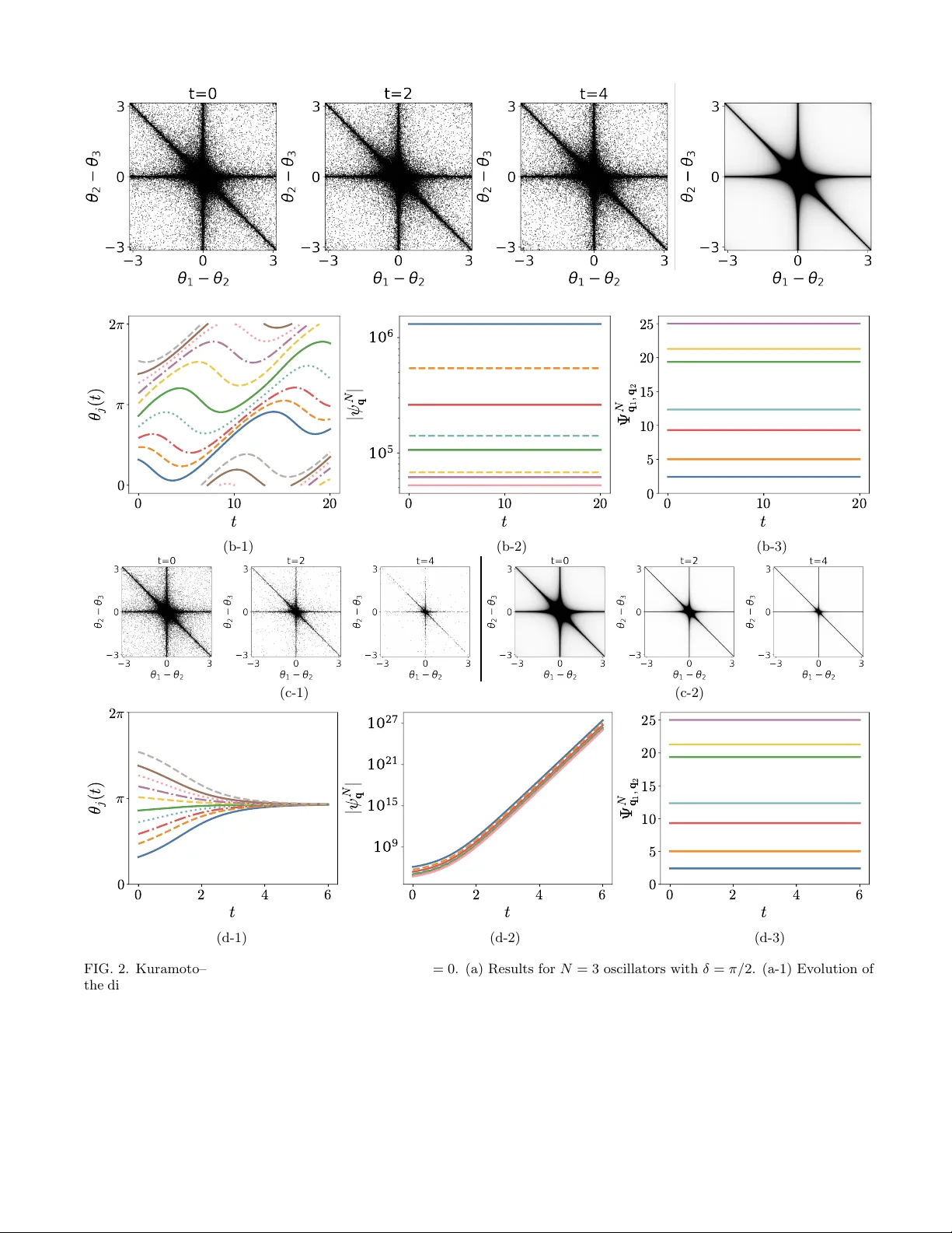
W atanab e–Strogatz In v arian ts in the Liouvillian Dynamics of Coupled Phase Oscillators via the Ko opman F ramew ork Keisuk e T aga 1 , and Hiro y a Nak ao 2 1 Dep artment of Physics and Astr onomy, T okyo University of Scienc e, Chib a 278-8510, Jap an 2 Dep artment of Systems and Contr ol Engine ering and R ese ar ch Center for Autonomous Systems Materialo gy, Institute of Scienc e T okyo, T okyo 152-8552, Jap an ∗ In dynamical systems, inv ariants, i.e., constants of motion conserved along the tra jectory , play imp ortan t roles in c haracterizing the system’s dynamical behavior. Recent applications of the Koop- man op erator framework to nonlinear dynamical systems hav e provided new insights in to the in- v ariants. F or a certain class of globally coupled phase oscillators, whic h serv e as mo dels for v arious sync hronization phenomena, W atanab e and Strogatz prov ed the existence of N − 3 inv ariants in N oscillator systems. In this study , w e derive these in v ariants from an op erator-theoretic persp ectiv e by exploiting the relation betw een Liouvillian (P erron–F rob enius) and Koopman descriptions of the dy- namics. Exploiting a simple multiplicativ e prop ert y of functions under the action of the Liouvillian and Ko opman operators, we explicitly construct a family of functions whose ratios yield the inv ari- an ts of the underlying dynamics. Our analysis successfully reproduces the full set of N − 3 in v arian ts kno wn in W atanabe–Strogatz theory , and offers an alternativ e sp ectral p erspective. W e demonstrate this approac h for a w ell-studied class of phase models, including the Ermen trout–Kop ell, pairwise Kuramoto, and higher-order Kuramoto mo dels. I. INTR ODUCTION Self-sustained oscillations are ubiquitous in the real world, including chemical oscillations [1 – 3], neuronal dynam- ics [4 – 6], circadian rh ythms [7, 8], and Josephson junction arra ys [9]. These oscillations emerge from v arious elementar y pro cesses, but they can often be reduced to one-dimensional dynamics b y fo cusing on their oscillation phases [2, 3, 10– 17]. A mathematical mo del that exclusively fo cuses on the phase dynamics of an oscillator is called a phase mo del [3]. In this study , we fo cus on a well-studied class of phase mo dels represented in the follo wing form: dθ dt = f ( t ) + g ( t ) cos θ + h ( t ) sin θ , (1a) where θ ( t ) ∈ [0 , 2 π ] is the oscillator phase (0 and 2 π are identified) at time t and f ( t ), g ( t ), and h ( t ) are smo oth functions of t . This class of systems has been studied extensiv ely since the pioneering w ork b y W atanabe and Strogatz [9, 18]. W e are typically in terested in a p opulation of globally coupled oscillators, where each oscillator obeys Eq. (1a) and interacts with other oscillators through the functions f , g , and h . The equation for the phase θ j ∈ [0 , 2 π ] of the j th oscillator ( j = 1 , . . . , N ), where N is the total num b er of oscillators, is then explicitly given by dθ j dt = f ( θ N , t ) + g ( θ N , t ) cos θ j + h ( θ N , t ) sin θ j , (1b) where θ N = ( θ 1 , θ 2 , . . . , θ N ). W ell-kno wn examples of globally coupled oscillators describ ed b y Eq. (1b) include the Winfree and Kuramoto mo dels [2, 3], which hav e b een extensively studied to inv estigate collective sync hronization phenomena in coupled-oscillator systems. F or N identical oscillators, b oth Eq. (1a) for indep endent oscillators and Eq. (1b) for coupled oscillators admit at least N − 3 inv ariants, i.e., constants of motion or conserved quantities, as shown by W atanab e and Strogatz in [18]. These in v ariants play an essen tial role in reducing the dimensionality and in establishing the integrabilit y of the system describ ed by Eq. (1a) or (1b). Using these inv arian ts, the N -dimensional dynamics of Eq. (1a) or (1b) can b e reduced to a system with only three degrees of freedom via the W atanab e–Strogatz transformation [18], which was later sho wn to b e a type of M¨ obius transformation [19]. This W atanab e–Strogatz framework for dimensionality reduction has since b een extended to phase-oscillator systems consisting of subp opulations [20, 21], under p erio dic forcing [22], high-dimensional Kuramoto mo dels [23], kinetic vector mo dels [24], and higher-order coupled models [25]. In addition, these in v arian ts are also analyzed from the p erspective of the Riccati equation [26] asso ciated with Eq. (1) [19, 27, 28]. ∗ tagakeisuk e@rs.tus.ac.jp 2 In this study , we explore the inv ariants of the ab ov e class of coupled-oscillator systems b y using the eigenfunctions of the Ko opman and Perron–F rob enius op erators, which are adjoint to each other. The Ko opman op erator [29–36] is a linear op erator that go verns the time ev olution of observ ables for dynamical systems, while the Perron–F rob enius op erator [31, 32, 36, 37] is a linear op erator describing the evolution of the state density of dynamical systems. This framew ork enables the study of nonlinear systems through linear techniques, suc h as sp ectral analysis. F or example, the dynamical properties of a system, including its inv arian ts, can b e characterized b y the eigenfunctions of the Ko opman op erator [12, 14, 33, 38 – 40]. Ko opman op erator theory has recently b een applied to analyze coupled phase oscillators in sev eral studies [41–45]. In this study , w e inv estigate the inv ariants of the systems given by Eq. (1a) or (1b) b y exploiting a simple relation that holds b etw een the Perron–F rob enius and Ko opman eigenfunctions. W e present a new path to deriving Ko opman eigenfunctions using Perron–F robenius eigenfunctions, which provides an alternativ e viewp oint on the inv ariants of globally coupled phase oscillators. I I. A GENERAL RELA TION BETWEEN PERR ON–FROBENIUS AND KOOPMAN EIGENFUNCTIONS A. Preliminaries F or a contin uous dynamical system of the form d x dt = F ( x , t ) , (2) where x ( t ) ∈ R N is the state of the system at time t and F ( x , t ) ∈ R N is the vector field representing the dynamics, the contin uous evolution of an observ able u ( x ) : R N → C is given by d dt u ( x ) = ( K u )( x ) = F ( x , t ) · ∇ u ( x ) , (3) where K = F ( x , t ) · ∇ is the infinitesimal generator of the Koopman operator (Koopman generator) [36] and ∇ = ∂ /∂ x represen ts the gradien t operator. The infinitesimal generator P of the P erron–F rob enius (PF) operator for con tinuous- time systems is the adjoint of K , P v ( x ) = −∇ · ( F ( x , t ) v ( x )) (4) whic h is also known as the Liouville op erator [36, 37, 46]. Here, the adjoint is defined with resp ect to the L 2 inner pro duct of tw o complex functions u ( x ) and v ( x ) on the state space (e.g., on the N -torus when x represents the phase v ariables), ⟨ u, K v ⟩ = ⟨P u, v ⟩ , ⟨ u, v ⟩ = Z u ( x ) v ( x ) d x , (5) where the ov erline indicates complex conjugate. While K describ es the time evolution of an observ able function, P has the physical meaning that it describ es the time evolution of a probability densit y function ρ ( x , t ) of the system state that is transp orted by the flo w generated by Eq. (2), which ob eys the Liouville equation, ∂ ∂ t ρ ( x , t ) = P ρ ( x , t ) . (6) W e note that the Ko opman and PF op erators can generally b e defined in the discrete-time setting, but we consider only their contin uous-time generators in this study . In what follo ws, w e refer to the eigenfunction u λ ( x ) and eigen v alue λ ∈ C of K satisfying K u λ ( x ) = λu λ ( x ) as the Ko opman eigenfunction and eigenvalue , and the eigenfunction v µ ( x ) and eigen v alue µ ∈ C of P satisfying P v µ ( x ) = µv µ ( x ) as the Perr on–F r ob enius (PF) eigenfunction and eigenvalue . Note that the eigenv alues of K and P are related through the adjointness [36]. In particular, from Eq. (3), a Ko opman eigenfunction with eigen v alue λ = 0 of K is an inv arian t of Eq. (2). W e b egin our analysis of the relationship b etw een the Ko opman and PF eigenfunctions for general dynamical systems given in the form of Eq. (2) with the follo wing lemma. Note that K and P are generally t -dep enden t. 3 Lemma 1. L et u 1 ( x ) and u 2 ( x ) b e sc alar-value d functions, wher e u 2 ( x ) /u 1 ( x ) is finite, and define two functions Λ 1 ( x , t ) := P u 1 ( x ) u 1 ( x ) , Λ 2 ( x , t ) := P u 2 ( x ) u 2 ( x ) . (7) Then the fol lowing identity holds: K  u 2 ( x ) u 1 ( x )  = { Λ 1 ( x , t ) − Λ 2 ( x , t ) } u 2 ( x ) u 1 ( x ) . (8) Pr o of. K  u 2 u 1  = F · ∇  u 2 u 1  = u 1 ( F · ∇ u 2 ) − u 2 ( F · ∇ u 1 ) u 2 1 = 1 u 2 1  u 1 {−P u 2 − ( ∇ · F ) u 2 } − u 2 {−P u 1 − ( ∇ · F ) u 1 }  = 1 u 2 1  u 1 ( −P u 2 ) − u 2 ( −P u 1 )  = (Λ 1 − Λ 2 ) u 2 u 1 . (9) Note that Λ 1 and Λ 2 are generally not eigen v alues of P as they are p oint-wise functions of x . F rom Lemma 1, w e immediately obtain the following theorem. Theorem 1. L et u 1 ( x ) and u 2 ( x ) b e gener al sc alar-value d functions satisfying P u 1 u 1 = P u 2 u 2 . (10) Then their r atio u 2 ( x ) /u 1 ( x ) is a Ko opman eigenfunction of K c orr esp onding to the eigenvalue 0 , and thus r epr esents an invariant of the system. Pr o of. Since P u 1 /u 1 = Λ 1 ( x , t ) = P u 2 /u 2 = Λ 2 ( x , t ), K  u 2 u 1  = { Λ 1 ( x , t ) − Λ 2 ( x , t ) } u 2 u 1 = 0 . (11) Theorem 2. L et u 1 ( x ) and u 2 ( x ) b e two PF eigenfunctions of P and λ 1 and λ 2 b e the c orr esp onding eigenvalues. Then their r atio u 2 ( x ) /u 1 ( x ) is a Ko opman eigenfunction of K with eigenvalue λ 1 − λ 2 . Pr o of. Since P u 1 ( x ) = λ 1 u 1 ( x ) and P u 2 ( x ) = λ 2 u 2 ( x ), Λ 1 ( x , t ) = λ 1 and Λ 2 ( x , t ) = λ 2 , hence K  u 2 u 1  = ( λ 1 − λ 2 ) u 2 u 1 . (12) Also, we obtain the following corollary . Corollary 1. Any r atio of two PF eigenfunctions asso ciate d with the same eigenvalue is an invariant of the system. Pr o of. If we assume λ 1 = λ 2 , K ( u 2 /u 1 ) = 0 and hence u 2 /u 1 is inv arian t. 4 I II. COUPLED PHASE OSCILLA TORS W e no w fo cus on a system of iden tical phase oscillators describ ed by Eq. (1b). The PF generator P of Eq. (1b) acts on a scalar function u ( θ N , t ) as P u := − N X j =1 ∂ ∂ θ j [( f + g cos θ j + h sin θ j ) u ] . (13) W e assume N ≥ 3 and in tro duce the following function: [55] ψ N q ( θ N ) := 1 Q N j =1 sin  θ q ( j ) − θ q ( j +1) 2  . (14) Here, the vector index q =  q (1) , q (2) , . . . , q ( N )  represen ts a p erm utation of the oscillator indices { 1 , 2 , . . . , N } , where q ( N +1) := q (1) . Theorem 3. By op er ating P on ψ N q , the fol lowing e quation holds: P ψ N q ( θ N ) = Λ( θ N , t ) ψ N q ( θ N ) , (15) wher e Λ( θ N , t ) := − N X j =1  ∂ f ( θ N , t ) ∂ θ j + cos θ j ∂ g ( θ N , t ) ∂ θ j + sin θ j ∂ h ( θ N , t ) ∂ θ j  . (16) Pr o of. See App endix A. Theorem 4. The r atio Ψ N q 1 , q 2 ( θ N ) := ψ N q 2 ( θ N ) ψ N q 1 ( θ N ) (17) is an eigenfunction of the asso ciate d Ko opman gener ator K c orr esp onding to eigenvalue 0 , and thus it serves as an invariant for Eq. (1) . Pr o of. P ψ N q 1 /ψ N q 1 = P ψ N q 2 /ψ N q 2 holds for any pair of p ermutations q 1 and q 2 b ecause Λ( θ N , t ) in Eq. (16) do es not dep end on the p erm utation q of the indices { 1 , 2 , . . . , N } . F rom Theorem 1, the ratio ψ N q 2 /ψ N q 1 is an eigenfunction of K with eigenv alue 0. W e hav e introduced ψ N q for N ≥ 3, but nontrivial inv ariants of the form Ψ N q 1 , q 2 arise only for N ≥ 4. When N = 3, ψ 3 q is the same for any p ermutation q , thus we hav e only a single trivial inv ariant Ψ 3 q 1 , q 2 = ± 1 (the sign dep ends on whether the p ermutations q 1 and q 2 are even or o dd). F or general N , the inv ariant Ψ N q 1 , q 2 can b e related to the kno wn in v arian ts, called cross ratios [19], and w e can show that the n umber of indep endent inv ariants of the form[56] Ψ N q 1 , q 2 is N − 3 except for a constant function, as shown in App endix B. Let us remark on the physical meaning of ψ N q ( θ N ) here. Supp ose that Λ( θ N , t ) = λ = const.. Then, ψ N q itself is a PF eigenfunction of P with eigenv alue λ . Since P describ es the evolution of the Liouville equation (6), ρ ( θ N , t ) = Ae λt ψ N q ( θ N ) (18) is a particular solution of Eq. (6), where A is an arbitrary constant. In particular, for the case of indep endent oscillators where eac h oscillator ob eys Eq. (1a) with f , g , and h dep ending only on time t , we obtain Λ( θ N , t ) = 0 in Eq. (16). Therefore, ψ N q is the PF eigenfunction with eigenv alue λ = 0 and thus it is a stationary solution of the Liouville equation (6), which can b e in terpreted as a stationary (unnormalized) density . Let us also remark that the mo dulus   ψ N q   of ψ N q has the same prop ert y as Eq. (15), i.e., P   ψ N q ( θ N )   = Λ( θ N , t )   ψ N q ( θ N )   , (19) 5 where Λ is giv en in Eq. (16). Therefore, we can rep eat the same argumen t as ab ov e also for   ψ N q   . In particular, if   ψ N q   is a PF eigenfunction of P , we obtain a particular solution of Eq. (6) as ρ ( θ N , t ) = Ae λt   ψ N q ( θ N )   . (20) In the numerical simulations presented b elo w, b ecause   ψ N q   is singular on [0 , 2 π ] N , we clip it and use the resulting function as a weigh ting function to sample the initial conditions. W e then simulate the evolution of the distribution of system states and compare it with the Liouvillian dynamics of the state density . In what follows, we present a few explicit examples that hav e b een well studied in the literature. W e consider the Ermen trout–Kop ell Theta model ( N oscillators without interaction) [6, 49], Kuramoto–Sak aguchi mo del ( N oscillators with pairwise in teraction) [2, 10], and higher-order (HO) Kuramoto mo del ( N oscillators with 3-b ody interaction) [50– 54]. In eac h case, w e focus on P ψ N q to see the difference b etw een the mo dels. As discussed ab ov e, Ψ N q 1 , q 2 is an inv ariant for each system. F or each system, we show the evolution of the system states for N = 3, where initial conditions are sampled according to the weigh t given by   ψ 3 q   . W e also show numerical e xamples of the time evolution of θ N , ψ N q , and Ψ N q 1 , q 2 with N = 10. A. Example 1. Ermen trout–Kop ell Theta mo del The Ermentrout–Kopell Theta mo del [6, 49] is a phase mo del of neuronal dynamics and also serves as the normal form of a saddle-no de bifurcation on an inv ariant circle. W e consider N uncoupled oscillators driven by a common input. The phase of eac h oscillator ob eys dθ j dt = 1 − cos θ j + (1 + cos θ j ) I ( t ) , (21) for j = 1 , ..., N , where I ( t ) is the common external input to the oscillator. Th us, the Theta mo del corresp onds to the case with f ( t ) = 1 + I ( t ), g ( t ) = − 1 + I ( t ), and h ( t ) = 0 in Eq. (1). Since f , g , and h are indep endent of the phases θ N = ( θ 1 , . . . , θ N ), all deriv ativ es in Eq. (16) v anish and hence Λ = 0 holds. Therefore, ψ N q ( θ N ) is a PF eigenfunction of this system with eigen v alue 0. By the metho d explained ab ov e, we can introduce N − 3 in v arian ts Ψ N q 1 , q 2 ( θ N ) from ψ N q 1 ( θ N ) and ψ N q 2 ( θ N ), where q 1 and q 2 are p erm utations of the oscillator indices { 1 , 2 , ..., N } . First, we consider N = 3 oscillators with I ( t ) = sin t as an example. Only one indep endent PF eigenfunction of the form ψ 3 q with q = (1 , 2 , 3) exists in this case. Figure 1(a) sho ws the evolution of the distribution of the phases θ 3 = ( θ 1 , θ 2 , θ 3 ) on the ( θ 1 − θ 2 ) − ( θ 2 − θ 3 ) plane obtained b y simulating the Theta mo del, Eq. (21), from 10 5 initial conditions. Here, the initial conditions w ere randomly sampled with weigh ts prop ortional to the PF eigenfunction   ψ 3 q ( θ 3 )   , whic h w as clipp ed at 10 2 b ecause   ψ 3 q ( θ 3 )   div erges when θ 1 = θ 2 , θ 2 = θ 3 , or θ 3 = θ 1 . The stationary solution   ψ 3 q ( θ 3 )   of the Liouville equation (6) giv en by Eq. (14) is shown on the same plane (also clipp ed at 10 2 and div ergent p oints are also plotted in black). In this example, the phase distribution on the ( θ 1 − θ 2 )–( θ 2 − θ 3 ) plane remains approximately stationary and is w ell captured by the stationary solution of the Liouville equation. Next, we consider the case with N = 10 and I ( t ) = sin t . Although the oscillators are uncoupled, the common time- dep enden t input en trains them, leading to phase locking with the input. In this case, w e can identify eight indep enden t functions of the form ψ 10 q ( θ 10 ( t )), from which N − 3 = 7 indep endent in v arian ts of the form Ψ 10 q 1 , q 2 ( θ 10 ( t )) can b e constructed. Figure 1(b) sho ws the time ev olution of (b-1) θ 10 ( t ) = ( θ 1 ( t ) , θ 2 ( t ) , . . . , θ 10 ( t )), (b-2)   ψ 10 q ( θ 10 ( t ))   , and (b-3)   Ψ 10 q 1 , q 2 ( θ 10 ( t ))   . W e can confirm that the ratio   Ψ 10 q 1 , q 2 ( θ 10 ( t ))   remains inv arian t under the non-stationary evolution of the phases θ 10 ( t ) = ( θ 1 ( t ) , θ 2 ( t ) , . . . , θ 10 ( t )). B. Example 2. Kuramoto–Sak aguchi Mo del The Kuramoto–Sak aguchi mo del [2, 10] describes a system of globally coupled oscillators. When all oscillators share the same frequency , the mo del is given by dθ j dt = ω + K N N X k =1 sin( θ k − θ j + δ ) , j = 1 , 2 , . . . , N , (22) where the parameters ω , K , and δ are the natural frequency , coupling intensit y , and coupling phase lag. 6 (a-1) (a-2) 0 5 1 0 t 0 π 2 π θ j ( t ) 0 5 1 0 t 1 0 8 1 0 1 3 1 0 1 8 1 0 2 3 | ψ N q | 0 5 1 0 t 0 5 1 0 1 5 2 0 2 5 | Ψ N q 1 , q 2 | (b-1) (b-2) (b-3) FIG. 1. Theta model with I ( t ) = sin t . (a) Results for N = 3 oscillators. (a-1) Evolution of the distribution of the phases θ 3 = ( θ 1 , θ 2 , θ 3 ) on the ( θ 1 − θ 2 ) − ( θ 2 − θ 3 ) plane, obtained by simulating the Theta mo del from 10 5 initial conditions sampled randomly with the w eights prop ortional to   ψ 3 q ( θ 3 )   (clipp ed at 10 2 ). Eac h black p oint corresp onds to a p oint θ 3 in the state space. (a-2) Densit y plot of   ψ 3 q ( θ 3 )   on the same plane, whic h is the stationary solution of the Liouville equation, clipped at 10 2 . V ertical, horizontal, and diagonal lines corresp ond to θ 1 = θ 2 , θ 2 = θ 3 , and θ 3 = θ 1 , whic h are singular points of   ψ 3 q ( θ 3 )   and also plotted in black. (b) Results for N = 10 oscillators. T ypical time evolution of the phases θ 10 ( t ) = ( θ 1 ( t ) , θ 2 ( t ) , . . . , θ 10 ( t )) (b-1),   ψ 10 q ( θ 10 ( t ))   (b-2), and   Ψ 10 q 1 , q 2 ( θ 10 ( t ))   (b-3) with time t . By transforming the right-hand side of Eq. (22), we obtain dθ j dt = ω + K N N X k =1 [sin( θ k + δ ) cos θ j − cos( θ k + δ ) sin θ j ] . (23) Th us, it has the form of Eq. (1b) with f ( θ N , t ) = ω , g ( θ N , t ) = K N N X k =1 sin( θ k + δ ) , h ( θ N , t ) = − K N N X k =1 cos( θ k + δ ) . (24) F rom these relations and Theorem 3, we obtain Λ = − K cos δ, (25) whic h is a constant that do es not dep end on θ N or t . Thus, ψ N q is a PF eigenfunction with eigen v alue − K cos δ . In particular, the case δ = π 2 (or equiv alently − π 2 ) is known to b e integrable [18]. In this case, the phase coupling b et w een the oscillators is neutral and mutual synchronization do es not o ccur for general N . Correspondingly , the 7 PF eigen v alue v anishes, i.e., Λ = − K cos δ = 0, and   ψ N q ( θ N )   corresp onds to a stationary solution of the Liouville equation. In this case, an y constant function c is also a PF eigenfunction with eigenv alue Λ = 0, b ecause P c = N X j =1 ∂ ∂ θ j " ω + K N N X k =1 cos( θ k − θ j ) # c = c K N N X j =1 N X k =1 [ − sin( θ k − θ j )] = 0 . (26) The ratio of ψ N q ( θ N ) to a constant function c is a Ko opman eigenfunction with eigenv alue 0, according to Theorem 2. Th us, by assuming c = 1, ψ N q ( θ N ) itself is found to b e a Ko opman eigenfunction. This inv ariant has previously b een found heuristically in [18]. Our framework provides an explanation for why such inv ariants emerge sp ecifically when δ = ± π 2 ; the constant function b ecomes a PF eigenfunction only in this case. Figure 2 sho ws the numerical results for N = 3 oscillators with K = 1, ω = 0, and δ = π 2 . In Fig. 2(a-1), ev olution of the distribution of the phases θ 3 = ( θ 1 , θ 2 , θ 3 ) is plotted on the ( θ 1 − θ 2 ) − ( θ 2 − θ 3 ) plane as b efore, whic h was obtained b y simulating the Kuramoto–Sak aguchi mo del from 10 5 initial conditions. The initial conditions w ere randomly sampled with weigh ts prop ortional to   ψ 3 q ( θ 3 )   (clipp ed at 10 2 ). Since Λ = 0 in this case, the phase distribution remains approximately stationary , and the oscillators do not tend to synchronize. In Fig. 2(a-2), the PF eigenfunction | ψ 3 q ( θ 3 ) | , which is a stationary solution of the Liouville equation, is plotted (also clipp ed at 10 2 ). The v ertical, horizon tal, and diagonal lines corresp ond to θ 1 = θ 2 , θ 2 = θ 3 , and θ 3 = θ 1 , resp ectively , whic h are singular p oin ts of   ψ 3 q ( θ 3 )   and plotted in black. The phase distributions in (a-1) agree well with the stationary state density in (a-2). Figure 2(b) shows the results for N = 10 oscillators, where time evolution of (b-1) the oscillator phases θ 10 ( t ) = ( θ 1 ( t ) , ..., θ 10 ( t )), (b-2)   ψ 10 q ( θ 10 ( t ))   , and (b-3) time ev olution of the ratio   Ψ 10 q 1 , q 2 ( θ 10 ( t ))   are plotted with resp ect to t . W e can confirm that the functions   ψ 10 q ( θ 10 ( t ))   , whic h are also Ko opman eigenfunctions, and   Ψ 10 q 1 , q 2 ( θ 10 ( t ))   remain constant under the non-stationary ev olution of θ 10 ( t ). Next, we consider the case δ = 0, where Eq. (22) is the standard Kuramoto mo del with a homogeneous frequency . In this case, all oscillator asymptotically synchronize completely , namely , lim t →∞ ( θ i ( t ) − θ j ( t )) = 0 for all i and j from almost all initial conditions. W e note that unstable phase-lo ck ed states also exist, which do not conv erge to complete synchronization. First, w e consider N = 3 oscillators with K = 1, ω = 0, and δ = 0. Figure 2(c-1) shows the evolution of the distribution of the phases θ 3 = ( θ 1 , θ 2 , θ 3 ) on the ( θ 1 − θ 2 ) − ( θ 2 − θ 3 ) plane as b efore, obtained by simulating the Kuramoto–Sak aguchi model, Eq. (22), from 10 5 initial conditions. Here, the initial conditions were randomly sampled with weigh ts prop ortional to the PF eigenfunction   ψ 3 q ( θ 3 )   (clipp ed at 10 2 ). Since the oscillators tend to sync hronize completely from almost all conditions in this case, the phase distribution tends to concentrate at the origin where θ 1 = θ 2 = θ 3 as t increases. The vertical, horizontal, and diagonal lines corresp ond to the states where t wo oscillators are synchronized ( θ 1 = θ 2 , θ 2 = θ 3 , or θ 3 = θ 1 ). Note that there are also unstable fixed p oints that do not con verge to complete synchronization on these lines. Figure 2(c-2) plots the evolution of the state density b y the Liouville equation (6), where the initial density is taken as the PF eigenfunction   ψ 3 q ( θ 3 )   . The solution is therefore given b y Ae − K t   ψ 3 q ( θ 3 )   , which decays exponentially with time t . The phase distribution in (c-1) and the state densit y in (c-2) agree well with each other. As the oscillators sync hronize m utually , the state densit y deca ys to zero at ev ery point in the state space, except on the vertical, horizon tal, or diagonal line where θ i = θ j for any pair of i, j = 1 , 2 , 3. Corresp ondingly , the PF eigenfunction ψ N q div erges when θ i = θ j for any i, j . The state density tends to accumulate on these singular sets, which corresp onds to the formation of synchronized clusters (i.e., at least some oscillators sharing the same phase). Then, the state densit y ev entually accum ulates at the origin, approaching the completely synchronized state. Note that there also exist singular p oints corresponding to the unstable solution that do not con verge to full synchron y . Figure 2(d) sho ws the time evolution of (d-1) θ 10 ( t ) = ( θ 1 ( t ) , θ 2 ( t ) , . . . , θ 10 ( t )), (d-2) | ψ 10 q ( θ 10 ( t )) | , and (d-3) | Ψ 10 q 1 , q 2 ( θ 10 ( t )) | . W e can confirm that the ratio | Ψ 10 q 1 , q 2 ( θ 10 ( t )) | remains in v ariant under the non-stationary ev olution of the phases θ 10 ( t ) = ( θ 1 ( t ) , θ 2 ( t ) , . . . , θ 10 ( t )). C. Example 3. Higher-order Kuramoto mo del As the last example, we consider a higher-order Kuramoto mo del. Recen tly , systems with higher-order interactions ha ve gained significan t atten tion due to their rich dynamical behaviors b eyond pairwise in teractions [25, 50 – 54]. Among several mo dels with higher-order interactions, w e consider the following Kuramoto-t yp e mo del [51–53]: dθ j dt = ω + K N 2 N X k,l =1 sin(2 θ k − θ l − θ j + δ ) . (27) 8 (a-1) (a-2) 0 1 0 2 0 t 0 π 2 π θ j ( t ) 0 1 0 2 0 t 1 0 5 1 0 6 | ψ N q | 0 1 0 2 0 t 0 5 1 0 1 5 2 0 2 5 Ψ N q 1 , q 2 (b-1) (b-2) (b-3) (c-1) (c-2) 0 2 4 6 t 0 π 2 π θ j ( t ) 0 2 4 6 t 1 0 9 1 0 1 5 1 0 2 1 1 0 2 7 | ψ N q | 0 2 4 6 t 0 5 1 0 1 5 2 0 2 5 Ψ N q 1 , q 2 (d-1) (d-2) (d-3) FIG. 2. Kuramoto–Sak aguchi model with K = 1 and ω = 0. (a) Results for N = 3 oscillators with δ = π/ 2. (a-1) Evolution of the distribution of the phases θ 3 = ( θ 1 , θ 2 , θ 3 ) on the ( θ 1 − θ 2 ) − ( θ 2 − θ 3 ) plane, obtained by sim ulating the Kuramoto–Sak aguchi mo del from 10 5 initial conditions randomly sampled as b efore. (a-2) Stationary state density   ψ 3 q ( θ 3 )   (clipp ed at 10 2 ) of the Liouville equation. (b) Results for N = 10 oscillators with δ = π / 2. Ev olution of the phases θ 10 ( t ) = ( θ 1 ( t ) , θ 2 ( t ) , . . . , θ 10 ( t )) (b-1),   ψ 10 q ( θ 10 ( t ))   (b-2), and   Ψ 10 q 1 , q 2 ( θ 10 ( t ))   (b-3) with time t . (c) Results for N = 3 oscillators with δ = 0. (c-1) Ev olution of the distribution of the phases θ 3 = ( θ 1 , θ 2 , θ 3 ) obtained by simulating the Kuramoto–Sak aguchi model from 10 5 initial conditions randomly sampled with weigh ts prop ortional to   ψ 3 q ( θ 3 )   (clipp ed at 10 2 ). Each black p oin t corresp onds to a p oint θ 3 in the state space. (c-2) Ev olution of the solution   ψ 3 q ( θ 3 )   e − K t (clipp ed at 10 2 ) of the Liouville equation. On the vertical, horizontal, and diagonal lines satisfying θ 1 = θ 2 , θ 2 = θ 3 , and θ 3 = θ 1 , resp ectiv ely , the solution diverges but is also plotted in black. (d) Results for N = 10 oscillators with δ = 0. Evolution of the phases θ 10 ( t ) = ( θ 1 ( t ) , θ 2 ( t ) , . . . , θ 10 ( t )) (d-1),   ψ 10 q ( θ 10 ( t ))   for (d-2), and   Ψ 10 q 1 , q 2 ( θ 10 ( t ))   (d-3) with time t . 9 The right-hand side of this equation can b e rewritten as dθ j dt = ω + K N 2 N X k,l =1  sin(2 θ k − θ l + δ ) cos θ j − cos(2 θ k − θ l + δ ) sin θ j  . (28) This corresp onds to the following case in Eq. (1b): f ( θ N , t ) = ω , g ( θ N , t ) = K N 2 N X k,l =1 sin(2 θ k − θ l + δ ) , h ( θ N , t ) = − K N 2 N X k,l =1 cos(2 θ k − θ l + δ ) . (29) Using the ab ov e relations, we obtain Λ( θ N ) = − 2 K R 2 1 ( θ N ) cos δ + K R 2 2 ( θ N ) cos δ, (30) where R 1 ( θ N ) is the Kuramoto order parameter [2] and R 2 ( θ N ) is the second order parameter [11] defined as R 1 ( θ N ) =       1 N N X j =1 e iθ j       , R 2 ( θ N ) =       1 N N X j =1 e i 2 θ j       . (31) These quantities c haracterize the degree of synchron y and tw o-cluster formation in the oscillator p opulation, and they are time-dep enden t functions in general. Therefore, for general δ , Λ is not constant and ψ N q is not a PF eigenfunction. Ho wev er, the ratio Ψ N q 1 , q 2 still forms an inv arian t by Theorem 1. Only when δ = ± π 2 , ψ N q b ecomes the PF eigenfunction with eigenv alue 0, namely , it gives a stationary distribution. Ho wev er, in contrast to the Kuramoto–Sak aguchi case, a constant function c is not a PF eigenfunction of this mo del. Indeed, introducing F j ( θ N ) := ω + K N 2 N X k,l =1 sin(2 θ k − θ l − θ j + δ ) , (32) w e obtain P c = − N X j =1 ∂ ∂ θ j  F j ( θ N ) c  = − c N X j =1 ∂ F j ( θ N ) ∂ θ j . (33) Th us, it follows that P c = Λ c ( θ N ) c with Λ c ( θ N ) = K N 2 N X j,k,l =1 cos(2 θ k − θ l − θ j + δ ) , (34) whic h generally dep ends on θ N . Hence c is not a PF eigenfunction. Figure 3(a) and (b) show the results for δ = π 2 . In Fig. 3(a-1), evolution of the distribution of the phases is plotted for N = 3, which is obtained by simulating the higher-order Kuramoto mo del from 10 5 initial conditions randomly sampled with w eights prop ortional to the PF eigenfunction   ψ 3 q ( θ 3 )   (clipp ed at 10 2 ). Since Λ = 0 in this case, the distribution remains appro ximately stationary . Figure 3(a-2) shows the stationary solution of the Liouville equation for N = 3, ψ 3 q ( θ 3 ). This function is divergen t on the horizon tal, v ertical, and diagonal lines, but is plotted in black as before. The phase distribution obtained b y simulating the higher-order Kuramoto model is in go o d agreement with the stationary solution   ψ 3 q ( θ 3 )   of the corresp onding Liouville equation. Figure 3(b) shows the results for N = 10, where time ev olution of phases θ 10 = ( θ 1 , θ 2 , . . . , θ 10 ) (b-1), tw o independent PF eigenfunctions   ψ 10 q ( θ 10 ( t ))   (b-2), and the ratio   Ψ 10 q 1 , q 2 ( θ 10 ( t ))   (b-3). The ratio Ψ 10 q 1 , q 2 ( θ 10 ( t )) remains inv arian t under the non-stationary evolution of the oscillator phases. W e also show the results for δ = 0, where the oscillators are asymptotically synchronized in Fig. 3(c). In this case, we see that   ψ 10 q ( θ 10 ( t ))   is not constant but the ratio Ψ 10 q 1 , q 2 ( θ 10 ( t )) remains inv ariant. 10 (a-1) (a-2) 0 2 0 4 0 t 0 π 2 π θ j ( t ) 0 2 0 4 0 t 1 0 5 1 0 6 1 0 7 | ψ N q | 0 2 0 4 0 t 0 5 1 0 1 5 2 0 2 5 Ψ N q 1 , q 2 (b-1) (b-2) (b-3) 0 2 0 4 0 t 0 π 2 π θ j ( t ) 0 2 0 4 0 t 1 0 8 1 0 1 4 1 0 2 0 1 0 2 6 1 0 3 2 | ψ N q | 0 2 0 4 0 t 0 5 1 0 1 5 2 0 2 5 Ψ N q 1 , q 2 (c-1) (c-2) (c-3) FIG. 3. Higher-order Kuramoto mo del with K = 1, ω = 0. (a) Results for N = 3 with δ = π / 2. (a-1) Evolution of the distribution of the phases θ 3 = ( θ 1 , θ 2 , θ 3 ) plotted on the ( θ 1 − θ 2 ) − ( θ 2 − θ 3 ) plane obtained by simulating the higher-order Kuramoto model from 10 5 random initial conditions sampled with the weigh ts prop ortional to   ψ 3 q ( θ 3 )   (clipp ed at 10 2 ). Eac h blac k p oin t corresp onds to a point θ 3 in the state space. (a-2) Stationary solution of the Liouville equation,   ψ 3 q ( θ 3 )   (clipp ed at 10 2 ). As before,   ψ 3 q ( θ 3 )   div erges on the vertical, horizon tal, and diagonal lines, but is plotted in black. (b) Results for N = 10 with δ = π / 2. Time evolution of the phases θ 10 ( t ) = ( θ 1 ( t ) , θ 2 ( t ) , . . . , θ 10 ( t )) (b-1),   ψ 10 q ( θ 10 ( t ))   (b-2), and   Ψ 10 q 1 , q 2 ( θ 10 ( t ))   (b-3) with time t . (c) Results for N = 10 with δ = 0. Time evolution of the phases θ 10 ( t ) = ( θ 1 ( t ) , θ 2 ( t ) , . . . , θ 10 ( t )) (c-1),   ψ 10 q ( θ 10 ( t ))   (c-2), and   Ψ 10 q 1 , q 2 ( θ 10 ( t ))   (c-3) with time t . IV. SUMMAR Y In this pap er, w e hav e exploited a simple relationship b et ween the Perron–F rob enius and Ko opman eigenfunctions for a certain class of many-bo dy oscillator systems describ ed b y phase mo dels to construct their inv arian ts from a sp ectral viewp oin t. By taking the ratios of the functions that share the same lo cal growth rate under the Liouvillian dynamics, we can systematically derive Ko opman eigenfunctions with zero eigenv alues, namely , the in v arian ts of the system dynamics. The resulting inv ariants coincide with those previously found through different metho ds. Thus, our 11 approac h gives a new, alternative framew ork for understanding the mathematical structure of in v arian ts in coupled- oscillator systems. Recen tly , W atanab e–Strogatz theory has been extended to Kuramoto mo dels defined on complex netw orks, enabling the analysis of in v arian ts in broader and more realistic settings [27]. Extending our framework to complex netw orks and systematically in v estigating the inv ariants through the Perron–F robenius and Ko opman eigenfunctions constitutes an interesting direction for future researc h. A cknow le dgements: K.T. ackno wledges JSPS KAKENHI 24K20863 for financial supp ort. H.N. ac knowledges JSPS KAKENHI 25H01468, 25K03081, 22K11919, and 22H00516 for financial supp ort. Data ac c essibility: This article has no additional data or co de. [1] Prigogine I, Lefever R. 1968 Symmetry Breaking Instabilities in Dissipativ e Systems. The Journal of Chemical Ph ysics 48 , 1695–1700. (10.1063/1.1668896) [2] Kuramoto Y. 1984 Chemical Oscillations, W av es, and T urbulence. New Y ork: Springer. [3] Winfree A T. 1967 Biological rhythms and the behavior of p opulations of coupled oscillators. Journal of Theoretical Biology 16 , 15–42. (10.1016/0022-5193(67)90051-3) [4] FitzHugh R. 1955 Mathematical mo dels of threshold phenomena in the nerve mem brane. Bulletin of Mathematical Bioph ysics 17 , 257–278. (10.1007/BF02477753) [5] Nagumo J, Arimoto S, Y oshizaw a S. 1962 An active pulse transmission line simulating nerve axon. Proceedings of the IRE 50 , 2061–2070. (10.1109/JRPR OC.1962.288235) [6] Ermentrout GB, Kop ell N. 1986 Parabolic bursting in an excitable system coupled with a slow oscillation. SIAM Journal on Applied Mathematics 46 , 233–253. (10.1137/0146017) [7] Goldb eter A. 1995 A mo del for circadian oscillations in the Drosophila p erio d protein (PER). Pro ceedings of the Roy al So ciet y B: Biological Sciences 261 , 319–324. (10.1098/rspb.1995.0153) [8] Kori H, Y amaguchi Y, Ok am ura H. 2017 Accelerating recov ery from jet lag: Prediction from a multi-oscillator mo del and its exp erimental confirmation in mo del animals. Journal of Biological Rhythms 32 , 44–58. (10.1177/0748730416671742) [9] W atanab e S, Strogatz SH. 1994 Constants of Motion for Sup erconducting Josephson Arrays. Ph ysica D 74 , 197–253. [10] Sak aguchi H, Kuramoto Y. 1986 A soluble activ e rotater mo del showing phase transitions via mutual entertainmen t. Progress of Theoretical Physics 76 , 576–581. (10.1143/PTP .76.576) [11] Daido H. 1992 Order function and macroscopic mutual entrainmen t in uniformly coupled limit-cycle oscillators. Progress of theoretical ph ysics 88 , 1213–1218. [12] Mauroy A, Mezi´ c I, Mo ehlis J. 2013 Isostables, Iso c hrons, and Koopman Sp ectrum for the Action–Angle Representation of Dynamical Systems. Physica D: Nonlinear Phenomena 261 , 19–30. (10.1016/j.physd.2013.06.015) [13] Nak ao H. 2016 Phase reduction approach to synchronisation of nonlinear oscillators. Con temp orary physics 57 , 188–214. [14] Shirasak a S, Kurebay ashi W, Nak ao H. 2017 Phase–Amplitude Reduction of T ransient Dynamics F ar from Attractors for Limit-Cycling Systems. Chaos 27 , 023119. (10.1063/1.4977728) [15] Y aw ata K, F uk ami K, T aira K, Nak ao H. 2024 Phase auto enco der for limit-cycle oscillators. Chaos: An Interdisciplinary Journal of Nonlinear Science 34 , 063111. (10.1063/5.0205718) [16] Namura N, Muolo R, Nak ao H. 2026 Optimal interaction functions realizing higher-order Kuramoto dynamics with arbitrary limit-cycle oscillators. Chaos: An Interdisciplinary Journal of Nonlinear Science 36 , 023120. (10.1063/5.0307452) [17] Ozaw a A, Kaw am ura Y. 2026 Phase reduction of reaction–diffusion systems with dela y . Chaos: An Interdisciplinary Journal of Nonlinear Science 36 , 033107. (10.1063/5.0313301) [18] W atanab e S, Strogatz SH. 1993 Integrabilit y of a Globally Coupled Oscillator Array . Physical Review Letters 70 , 2391– 2394. (10.1103/PhysRevLett.70.2391) [19] Marvel SA, Mirollo RE, Strogatz SH. 2009 Identical Phase Oscillators with Global Sinusoidal Coupling Ev olve by M¨ obius Group Action. Chaos 19 , 043104. (10.1063/1.3247089) [20] Piko vsky A, Rosen blum M. 2008 P artially Integrable Dynamics of Hierarc hical Populations of Coupled Oscillators. Ph ysical Review Letters 101 , 264103. (10.1103/Ph ysRevLett.101.264103) [21] Hong H, Strogatz SH. 2011 Conformists and contrarians in a Kuramoto mo del with identical natural frequencies. Phys. Rev. E 84 , 046202. (10.1103/Ph ysRevE.84.046202) [22] Atsumi Y, Nak ao H. 2012 Persisten t fluctuations in synchronization rate in globally coupled oscillators with perio dic external forcing. Ph ysical Review E—Statistical, Nonlinear, and Soft Matter Ph ysics 85 , 056207. [23] Lohe MA. 2018 Higher-dimensional generalizations of the W atanabe–Strogatz transform for vector mo dels of sync hroniza- tion. Journal of Physics A: Mathematical and Theoretical 51 , 225101. (10.1088/1751-8121/aac030) [24] Park H. 2022 The W atanab e-Strogatz transform and constant of motion functionals for kinetic vector mo dels. Journal of Differen tial Equations 323 , 113–151. (https://doi.org/10.1016/j.jde.2022.03.027) [25] Jain JC, Jalan S. 2025 Low-dimensional W atanabe–Strogatz approach for Kuramoto oscillators with higher-order in terac- tions. Chaos: An Interdisciplinary Journal of Nonlinear Science 35 , 091104. (10.1063/5.0283600) [26] Reid WT. 1972 Riccati Differential Equations. New Y ork: Academic Press. [27] Cestnik R, Martens EA. 2024 Integrabilit y of a Globally Coupled Complex Riccati Array: Quadratic Integrate-and-Fire Neurons, Phase Oscillators, and All in Betw een. Physical Review Letters 132 , 057201. (10.1103/PhysRevLett.132.057201) 12 [28] Paz´ o D, Cestnik R. 2025 Lo w-dimensional dynamics of globally coupled complex Riccati equations: Exact firing-rate equations for spiking neurons with clustered substructure. Phys. Rev. E 111 , L052201. (10.1103/PhysRevE.111.L052201) [29] Ko opman BO. 1931 Hamiltonian Systems and T ransformation in Hilb ert Space. Pro ceedings of the National Academ y of Sciences 17 , 315–318. (10.1073/pnas.17.5.315) [30] Ko opman BO, von Neumann J. 1932 Dynamical Systems of Con tinuous Sp ectra. Proceedings of the National Academy of Sciences 18 , 255–263. (10.1073/pnas.18.3.255) [31] Lasota A, Mack ey MC. 2013 Chaos, fractals, and noise: sto chastic aspects of dynamics vol. 97. Springer Science & Business Media. [32] Mezi´ c I. 2005 Sp ectral Prop erties of Dynamical Systems, Mo del Reduction and Decomp ositions. Nonlinear Dynamics 41 , 309–325. (10.1007/s11071-005-2824-x) [33] Budi ˇ si ´ c M, Mohr R, Mezi´ c I. 2012 Applied koopmanism. Chaos: An Interdisciplinary Journal of Nonlinear Science 22 . [34] Mezi´ c I. 2013 Analysis of fluid flows via sp ectral prop erties of the Koopman op erator. Annual review of fluid mechanics 45 , 357–378. [35] Mauroy A, Susuki Y, Mezi´ c I. 2020 The Ko opman Op erator in Systems and Con trol. Springer. [36] Brunton SL, Budi ˇ si ´ c M, Kaiser E, Kutz JN. 2022 Mo dern Ko opman Theory for Dynamical Systems. SIAM Review 64 , 229–340. (10.1137/21M1425367) [37] Gaspard P . 1998 Chaos, Scattering and Statistical Mechanics. Cambridge Nonlinear Science Series. Cambridge Univ ersity Press. [38] T aga K, Kato Y, Kaw ahara Y, Y amazaki Y, Nak ao H. 2021 Ko opman sp ectral analysis of elementary cellular automata. Chaos: An Interdisciplinary Journal of Nonlinear Science 31 . [39] Park er JP , V alv a C. 2023 Ko opman analysis of the p eriodic Korteweg–de V ries equation. Chaos: An In terdisciplinary Journal of Nonlinear Science 33 . [40] T aga K, Kato Y, Y amazaki Y, Kaw ahara Y, Nak ao H. 2024 Dynamic mo de decomp osition for Ko opman spectral analysis of elementary cellular automata. Chaos: An Interdisciplinary Journal of Nonlinear Science 34 . [41] Susuki Y, Mezic I, Raak F, Hikihara T. 2016 Applied Ko opman op erator theory for p ow er systems tec hnology . Nonlinear Theory and Its Applications, IEICE 7 , 430–459. (10.1587/nolta.7.430) [42] Hu J, Lan Y. 2020 Ko opman analysis in oscillator synchronization. Phys. Rev. E 102 , 062216. (10.1103/Phys- RevE.102.062216) [43] W ang S, Lan Y. 2021 Probing the Phase Space of Coupled Oscillators with Ko opman Analysis. Physical Review E 104 , 034211. (10.1103/PhysRevE.104.034211) [44] Mihara A, Zaks M, Macau EEN, Medrano-T RO. 2022 Basin sizes dep end on stable eigenv alues in the Kuramoto mo del. Ph ys. Rev. E 105 , L052202. (10.1103/Ph ysRevE.105.L052202) [45] Thib eault V, Clav eau B, Allard A, Desrosiers P . 2025 Kuramoto meets Ko opman: Constants of motion, symmetries, and net work motifs. arXiv preprin t [46] Kato Y, Zhu J, Kureba yashi W, Nak ao H. 2021 Asymptotic phase and amplitude for classical and semiclassical sto c hastic oscillators via Ko opman op erator theory . Mathematics 9 , 2188. [47] Note1. W e note that ψ N q / ∈ L 2 ([0 , 2 π ] N ) b ecause it div erges when θ q ( j ) = θ q ( j +1) , which can occur when θ i = θ j for some ( i, j ). In practice, we therefore consider a domain that excludes neighborho ods of these collision sets, for instance X ε = { ( θ 1 , . . . , θ N ) | | θ i − θ j | > ε for all i  = j } with some ε > 0. F or iden tical oscillators evolving under a smo oth vector field, the induced flo w is unique and inv ertible for any finite time; hence phases cannot coincide in finite time unless they coincide initially . W e use X ε whenev er needed to k eep ψ N q w ell behav ed. [48] Note2. W e note that other inv arian ts that do not take the form of the cross ratio can also exist; see the examples of the Theta mo del in App endix C. [49] Ermentrout B. 2008 Ermentrout-Kopell canonical mo del. Scholarpedia 3 , 1398. (10.4249/sc holarp edia.1398) [50] T anak a T, Aoy agi T. 2011 Multistable attractors in a netw ork of phase oscillators with three-b ody interactions. Physical Review Letters 106 , 224101. [51] Sk ardal PS, Arenas A. 2020 Higher-order interactions in complex netw orks of phase oscillators promote abrupt synchro- nization switching. Communications Ph ysics 3 , 218. (10.1038/s42005-020-00485-0) [52] Le´ on I, Muolo R, Hata S, Nak ao H. 2024 Higher-order interactions induce anomalous transitions to synchron y . Chaos 34 , 013105. (10.1063/5.0172585) [53] Le´ on I, Muolo R, Hata S, Nak ao H. 2025 Theory of phase reduction from h yp ergraphs to simplicial com- plexes: A general route to higher-order Kuramoto mo dels. Physica D: Nonlinear Phenomena p. 134858. (h ttps://doi.org/10.1016/j.physd.2025.134858) [54] F ujii N, T aga K, Muolo R, Rink B, Nak ao H. 2025 Emergence of higher-order interactions in systems of coupled Kuramoto oscillators with time delay . arXiv preprint [55] W e note that ψ N q / ∈ L 2 ([0 , 2 π ] N ) b ecause it div erges when θ q ( j ) = θ q ( j +1) , which can o ccur when θ i = θ j for some ( i, j ). In practice, we therefore consider a domain that excludes neighborho ods of these collision sets, for instance X ε = { ( θ 1 , . . . , θ N ) | | θ i − θ j | > ε for all i  = j } with some ε > 0. F or identical oscillators evolving under a smo oth v ector field, the induced flo w is unique and in v ertible for an y finite time; hence phases cannot coincide in finite time unless they coincide initially . W e use X ε whenev er needed to k eep ψ N q w ell behav ed. [56] W e note that other in v arian ts that do not take the form of the cross ratio can also exist; see the examples of the Theta mo del in App endix C. 13 App endix A: Pro of of Theorem 3 W e compute each term included in P ψ N q of Eq. (15). The first term inv olving f can b e expanded as N X j =1 ∂ ( f ψ N q ) ∂ θ j = ψ N q N X j =1  ∂ f ∂ θ j + f 2  cot  θ q ( j − 1) − θ q ( j ) 2  − cot  θ q ( j ) − θ q ( j +1) 2   = ψ N q N X j =1 ∂ f ∂ θ j . (A1) In the ab ov e equation, the term {· · · } v anishes due to the cyclic sum. Similarly , the second g cos θ j term can b e calculated as N X j =1 ∂ g cos θ j ψ N q ∂ θ j = ψ N q N X j =1  ∂ g ∂ θ j cos θ j + g  − sin θ j + 1 2 cos θ q ( j )  cot  θ q ( j − 1) − θ q ( j ) 2  − cot  θ q ( j ) − θ q ( j +1) 2   = ψ N q N X j =1 cos θ j ∂ g ∂ θ j , (A2) where the term {· · · } v anishes b ecause of the trigonometric prop erty N X j =1 cos θ q ( j )  cot  θ q ( j − 1) − θ q ( j ) 2  − cot  θ q ( j ) − θ q ( j +1) 2  = − N X j =1 (cos θ q ( j − 1) − cos θ q ( j ) ) cot  θ q ( j − 1) − θ q ( j ) 2  = N X j =1 2 sin  θ q ( j − 1) + θ q ( j ) 2  sin  θ q ( j − 1) − θ q ( j ) 2  cot  θ q ( j − 1) − θ q ( j ) 2  = N X j =1 2 sin  θ q ( j − 1) + θ q ( j ) 2  cos  θ q ( j − 1) − θ q ( j ) 2  = N X j =1 [sin θ q ( j − 1) + sin θ q ( j ) ] (A3) and the cyclic sum, N X j =1  − sin θ j + 1 2  sin θ q ( j − 1) + sin θ q ( j )   = 0 . (A4) F or the last h sin θ j term, we obtain N X j =1 ∂ h sin θ j ψ N q ∂ θ j = ψ N q N X j =1  ∂ h ∂ θ j sin θ j + h  cos θ j + 1 2 sin θ q ( j )  cot  θ q ( j − 1) − θ q ( j ) 2  − cot  θ q ( j ) − θ q ( j +1) 2   = ψ N q N X j =1 ∂ h ∂ θ j sin θ j . (A5) 14 Again, the term {· · · } v anishes b ecause of the trigonometric prop erty N X j =1 sin θ q ( j )  cot  θ q ( j − 1) − θ q ( j ) 2  − cot  θ q ( j ) − θ q ( j +1) 2  = − N X j =1  sin θ q ( j − 1) − sin θ q ( j )  cot  θ q ( j − 1) − θ q ( j ) 2  = − N X j =1 2 cos  θ q ( j − 1) + θ q ( j ) 2  sin  θ q ( j − 1) − θ q ( j ) 2  cot  θ q ( j − 1) − θ q ( j ) 2  = − N X j =1 2 cos  θ q ( j − 1) + θ q ( j ) 2  cos  θ q ( j − 1) − θ q ( j ) 2  = − N X j =1  cos θ q ( j − 1) + cos θ q ( j )  (A6) and the cyclic sum, N X j =1  cos θ j − 1 2  cos θ q ( j − 1) + cos θ q ( j )   = 0 . (A7) Com bining all the terms, w e obtain P ψ N q ( θ N ) = Λ( θ N , t ) ψ N q ( θ N ) , (A8) where Λ( θ N , t ) := − N X j =1  ∂ f ( θ N , t ) ∂ θ j + cos θ j ∂ g ( θ N , t ) ∂ θ j + sin θ j ∂ h ( θ N , t ) ∂ θ j  . (A9) App endix B: Indep enden t Inv arian ts 1. Riccati equation and cross ratios W e here discuss the relation of the inv arian ts with the Riccati equation. While the N − 3 inv ariants of Eq. (1a) or (1b) were originally found by the W atanab e–Strogatz transformation, they can also b e obtained from the prop erty of the Riccati equation into whic h Eq. (1a) can b e transformed [9, 19]. The Riccati equation [26] is a nonlinear ordinary differential equation defined as dx dt = α ( t ) x + β ( t ) x 2 + γ ( t ) , (B1) where α ( t ), β ( t ), and γ ( t ) are time-dependent functions. Notably , giv en four distinct solutions to the Riccati equation, one can construct an inv ariant quantit y termed cr oss r atio [26], expressed as follo ws: ( x 1 − x 2 )( x 3 − x 4 ) ( x 2 − x 3 )( x 4 − x 1 ) . (B2) Here, x 1 ( t ), x 2 ( t ), x 3 ( t ), and x 4 ( t ) are the solutions of Eq. (B1) with distinct initial conditions x 1 (0), x 2 (0), x 3 (0), and x 4 (0). Equation (1a) is transformed into the form of a Riccati equation by considering the time ev olution of the complex v ariable x = e iθ [9, 19]: dx dt = d dt e iθ = i ( f ( t ) + g ( t ) cos θ + h ( t ) sin θ ) e iθ = if ( t ) x + i 2 ( g ( t ) + ih ( t )) x 2 + i 2 ( g ( t ) − ih ( t )) . (B3) 15 Therefore, Eq. (1a) corresp onds to the Riccati equation (B1) with the following co efficients: α ( t ) = if ( t ) , β ( t ) = i 2 ( g ( t ) + ih ( t )) , γ ( t ) = i 2 ( g ( t ) − ih ( t )) . (B4) It follows that, for four distinct solutions θ 1 , θ 2 , θ 3 , and θ 4 of Eq. (1a), the following quan tity: ( e iθ 1 − e iθ 2 )( e iθ 3 − e iθ 4 ) ( e iθ 2 − e iθ 3 )( e iθ 4 − e iθ 1 ) (B5) is an inv ariant. The cross ratio in Eq. (B2) can b e equiv alen tly rewritten in terms of sine functions as (see [19]) ⟨ 1 , 2 , 3 , 4 ⟩ = sin  θ 1 − θ 2 2  sin  θ 3 − θ 4 2  sin  θ 2 − θ 3 2  sin  θ 4 − θ 1 2  , (B6) where w e introduced the notation ⟨ i, j, k , l ⟩ for the cross ratio. F rom N distinct solutions of Eq. (1a), one can construct N ( N − 1)( N − 2)( N − 3) (the total num b er of ordered four indices) such inv ariants of the form ⟨ i, j, k , l ⟩ , but only N − 3 of them are indep enden t functions [19]. 2. P erron–F robenius eigenfunctions and an inv arian t for N = 4 Before we discuss the relation b et w een the WS inv ariants and Ψ N q 1 , q 2 , w e sho w that only one functionally indep endent in v arian t given in the form Ψ 4 q 1 , q 2 exists when N = 4. The function ψ 4 q satisfies the following cyclic symmetry: ψ 4 ( q (1) ,q (2) ,q (3) ,q (4) ) = ψ 4 ( q (2) ,q (3) ,q (4) ,q (1) ) = ψ 4 ( q (3) ,q (4) ,q (1) ,q (2) ) = ψ 4 ( q (4) ,q (1) ,q (2) ,q (3) ) , (B7) and reversal symmetry: ψ 4 ( q (1) ,q (2) ,q (3) ,q (4) ) = ψ 4 ( q (4) ,q (3) ,q (2) ,q (1) ) . (B8) Giv en these symmetries, only three functions remain: ψ 4 (1 , 2 , 3 , 4) , ψ 4 (1 , 3 , 4 , 2) , ψ 4 (1 , 4 , 2 , 3) . (B9) In addition, one more relation exists: ψ 4 (1 , 2 , 3 , 4) + ψ 4 (1 , 3 , 4 , 2) + ψ 4 (1 , 4 , 2 , 3) = 0 , (B10) namely , only tw o of the functions in Eq. (B9) are indep enden t, such as ψ 4 (1 , 2 , 3 , 4) , ψ 4 (1 , 3 , 4 , 2) . (B11) F rom these functions, we can construct only one indep enden t inv arian t Ψ 4 (1 , 2 , 3 , 4) , (1 , 3 , 4 , 2) . 3. Relationship b et ween Ψ N q and ⟨ i, j, k , l ⟩ Here, we sho w that the set Ψ N = { Ψ N q 1 , q 2 } q 1 , q 2 includes all in v arian ts of the form ⟨ q (1) , q (2) , q (3) , q (4) ⟩ , introduced in Eq. (B6), and that each function Ψ N q 1 , q 2 can b e decomp osed into a pro duct of suc h terms. Consequently , the num b er of indep enden t inv ariants in Ψ N is N − 3 (except for a constant function, which is a trivial inv ariant). Our discussion is as follows. W e compare inv ariants in Ψ N with ⟨ i, j, k , l ⟩ , and, using the fact that the num b er of indep enden t functions of ⟨ i, j , k , l ⟩ is N − 3 [19], w e sho w that the num b er of functions in Ψ N is also N − 3. T o this end, we show that inv ariants in Ψ N can b e constructed as products of ⟨ i, j, k , l ⟩ . First, we show that Ψ 4 coincides with ⟨ i, j, k , l ⟩ . Then, for N ≥ 5, we sho w that Ψ N can b e expressed as Ψ N − 1 m ultiplied by sev eral terms of ⟨ i, j, k , l ⟩ . 16 It follows that any Ψ N can b e expressed as a pro duct of ⟨ i, j, k , l ⟩ , implying that the n umber of independent Ψ N is at most N − 3. Next, we sho w that the set of Ψ N includes ⟨ i, j, k , l ⟩ . This implies that the n umber of indep enden t Ψ N is at least N − 3. Combining these results, we conclude that the num b er of indep enden t Ψ N is exactly N − 3. W e utilize the symmetric prop erties of the cross ratio ⟨ i, j, k , l ⟩ [19] that any p ermutation of the four indices yields an expression functionally depe nden t on ⟨ i, j, k , l ⟩ . That is, all such v arian ts can b e written as rational functions of a single cross ratio and thus they are not indep enden t. W e b egin with the case N = 4. As we discussed in App endix B 2, only one indep endent in v arian t can b e obtained as Ψ 4 q 1 , q 2 in this case. Let us choose Ψ 4 (1 , 3 , 4 , 2) , (1 , 4 , 2 , 3) as the represen tative one. By calculating the fraction, we obtain the following relation: Ψ 4 (1 , 3 , 4 , 2) , (1 , 4 , 2 , 3) = ψ 4 (1 , 4 , 2 , 3) ψ 4 (1 , 3 , 4 , 2) = sin  θ 1 − θ 3 2  sin  θ 3 − θ 4 2  sin  θ 4 − θ 2 2  sin  θ 2 − θ 1 2  sin  θ 1 − θ 4 2  sin  θ 4 − θ 2 2  sin  θ 2 − θ 3 2  sin  θ 3 − θ 1 2  = − sin  θ 1 − θ 2 2  sin  θ 3 − θ 4 2  sin  θ 2 − θ 3 2  sin  θ 4 − θ 1 2  = −⟨ 1 , 2 , 3 , 4 ⟩ . (B12) Though not indep endent of Eq. (B12), we note that Ψ 4 (1 , 4 , 2 , 3) , (1 , 2 , 3 , 4) and Ψ 4 (1 , 2 , 3 , 4) , (1 , 3 , 4 , 2) can also b e constructed as the ratio of ψ 4 q and ψ 4 q ′ with different p ermutation q and q ′ , and we can find the following relations: Ψ 4 (1 , 4 , 2 , 3) , (1 , 2 , 3 , 4) = −⟨ 1 , 3 , 4 , 2 ⟩ , (B13) Ψ 4 (1 , 2 , 3 , 4) , (1 , 3 , 4 , 2) = −⟨ 1 , 4 , 2 , 3 ⟩ . (B14) Then, let us consider the case N ≥ 5. Lemma 2. L et N ≥ 5 , and let Ψ N q 1 , q 2 b e define d as b efor e. Then Ψ N q 1 , q 2 c an b e r e duc e d to Ψ N − 1 q ′ 1 , q ′ 2 or de c omp ose d as a pr o duct of Ψ N − 1 q ′ 1 , q ′ 2 and invariants ⟨ i, j, k , l ⟩ . Her e, q ′ 1 , q ′ 2 ar e the p ermutations of { 1 , 2 , . . . , N − 1 } obtaine d by r emoving N fr om q 1 and q 2 : q ′ ( l ) 1 = ( q ( l ) 1 , if l < ξ , q ( l +1) 1 , if l ≥ ξ , q ′ ( l ) 2 = ( q ( l ) 2 , if l < ζ , q ( l +1) 2 , if l ≥ ζ , (B15) wher e q ( ξ ) 1 = q ( ζ ) 2 = N , and we imp ose the cyclic pr op erty in the indic es as q (0) 1 , 2 = q ( N ) 1 , 2 and q ( N +1) 1 , 2 = q (1) 1 , 2 . Pr o of. F rom Eq. (14), we can decomp ose Ψ N q 1 , q 2 as Ψ N q 1 , q 2 = Ψ N − 1 q ′ 1 , q ′ 2 sin  θ q ( ξ − 1) 1 − θ q ( ξ ) 1 2  sin  θ q ( ξ ) 1 − θ q ( ξ +1) 1 2  sin  θ q ( ζ − 1) 2 − θ q ( ζ ) 2 2  sin  θ q ( ζ ) 2 − θ q ( ζ +1) 2 2  · sin  θ q ( ζ − 1) 2 − θ q ( ζ +1) 2 2  sin  θ q ( ξ − 1) 1 − θ q ( ξ +1) 1 2  . (B16) W e analyze this by dividing into the following six cases. Case.1: { q ( ξ − 1) 1 , q ( ξ +1) 1 } = { q ( ζ − 1) 2 , q ( ζ +1) 2 } In this case, the following equation holds: sin  θ q ( ξ − 1) 1 − θ q ( ξ ) 1 2  sin  θ q ( ξ ) 1 − θ q ( ξ +1) 1 2  sin  θ q ( ζ − 1) 2 − θ q ( ζ ) 2 2  sin  θ q ( ζ ) 2 − θ q ( ζ +1) 2 2  = 1 . (B17) Th us, we obtain Ψ N q 1 , q 2 = Ψ N − 1 q ′ 1 , q ′ 2 . (B18) This includes b oth the aligned case ( q ( ξ − 1) 1 , q ( ξ +1) 1 ) = ( q ( ζ − 1) 2 , q ( ζ +1) 2 ) and the swapped case ( q ( ξ − 1) 1 , q ( ξ +1) 1 ) = ( q ( ζ +1) 2 , q ( ζ − 1) 2 ), and in either situation the sine factors cancel pairwise, yielding the ratio 1. 17 Case.2: q ( ξ − 1) 1 = q ( ζ − 1) 2 = M , q ( ξ +1) 1  = q ( ζ +1) 2 In this case, the following relation holds: sin  θ q ( ξ − 1) 1 − θ q ( ξ ) 1 2  sin  θ q ( ξ ) 1 − θ q ( ξ +1) 1 2  sin  θ q ( ζ − 1) 2 − θ q ( ζ +1) 2 2  sin  θ q ( ζ − 1) 2 − θ q ( ζ ) 2 2  sin  θ q ( ζ ) 2 − θ q ( ζ +1) 2 2  sin  θ q ( ξ − 1) 1 − θ q ( ξ +1) 1 2  = sin  θ q ( ξ ) 1 − θ q ( ξ +1) 1 2  sin  θ q ( ζ − 1) 2 − θ q ( ζ +1) 2 2  sin  θ q ( ζ ) 2 − θ q ( ζ +1) 2 2  sin  θ q ( ξ − 1) 1 − θ q ( ξ +1) 1 2  = sin  θ N − θ q ( ξ +1) 1 2  sin  θ M − θ q ( ζ +1) 2 2  sin  θ N − θ q ( ζ +1) 2 2  sin  θ M − θ q ( ξ +1) 1 2  = ⟨ N , q ( ξ +1) 1 , M , q ( ζ +1) 2 ⟩ . (B19) Th us, we obtain Ψ N q 1 , q 2 = Ψ N − 1 q ′ 1 , q ′ 2 ⟨ N , q ( ξ +1) 1 , M , q ( ζ +1) 2 ⟩ . (B20) Case.3: q ( ξ +1) 1 = q ( ζ +1) 2 = M , q ( ξ − 1) 1  = q ( ζ − 1) 2 In this case, the following relation holds: sin  θ q ( ξ − 1) 1 − θ q ( ξ ) 1 2  sin  θ q ( ξ ) 1 − θ q ( ξ +1) 1 2  sin  θ q ( ζ − 1) 2 − θ q ( ζ +1) 2 2  sin  θ q ( ζ − 1) 2 − θ q ( ζ ) 2 2  sin  θ q ( ζ ) 2 − θ q ( ζ +1) 2 2  sin  θ q ( ξ − 1) 1 − θ q ( ξ +1) 1 2  = sin  θ q ( ξ − 1) 1 − θ q ( ξ ) 1 2  sin  θ q ( ζ − 1) 2 − θ q ( ζ +1) 2 2  sin  θ q ( ζ − 1) 2 − θ q ( ζ ) 2 2  sin  θ q ( ξ − 1) 1 − θ q ( ξ +1) 1 2  = sin  θ q ( ξ − 1) 1 − θ N 2  sin  θ q ( ζ − 1) 2 − θ M 2  sin  θ q ( ζ − 1) 2 − θ N 2  sin  θ q ( ξ − 1) 1 − θ M 2  = ⟨ N , q ( ξ − 1) 1 , M , q ( ζ − 1) 2 ⟩ . (B21) Th us, we obtain Ψ N q 1 , q 2 = Ψ N − 1 q ′ 1 , q ′ 2 ⟨ N , q ( ξ − 1) 1 , M , q ( ζ − 1) 2 ⟩ . (B22) Case.4: q ( ξ − 1) 1 = q ( ζ +1) 2 = M , q ( ξ +1) 1  = q ( ζ − 1) 2 18 In this case, the following relation holds: sin  θ q ( ξ − 1) 1 − θ q ( ξ ) 1 2  sin  θ q ( ξ ) 1 − θ q ( ξ +1) 1 2  sin  θ q ( ζ − 1) 2 − θ q ( ζ +1) 2 2  sin  θ q ( ζ − 1) 2 − θ q ( ζ ) 2 2  sin  θ q ( ζ ) 2 − θ q ( ζ +1) 2 2  sin  θ q ( ξ − 1) 1 − θ q ( ξ +1) 1 2  = − sin  θ q ( ξ ) 1 − θ q ( ξ +1) 1 2  sin  θ q ( ζ − 1) 2 − θ q ( ζ +1) 2 2  sin  θ q ( ζ − 1) 2 − θ q ( ζ ) 2 2  sin  θ q ( ξ − 1) 1 − θ q ( ξ +1) 1 2  = − sin  θ N − θ q ( ξ +1) 1 2  sin  θ q ( ζ − 1) 2 − θ M 2  sin  θ q ( ζ − 1) 2 − θ N 2  sin  θ M − θ q ( ξ +1) 1 2  = −⟨ N , q ( ξ +1) 1 , M , q ( ζ − 1) 2 ⟩ . (B23) Th us, we obtain Ψ N q 1 , q 2 = − Ψ N − 1 q ′ 1 , q ′ 2 ⟨ N , q ( ξ +1) 1 , M , q ( ζ − 1) 2 ⟩ . (B24) Case.5: q ( ξ +1) 1 = q ( ζ − 1) 2 = M , q ( ξ − 1) 1  = q ( ζ +1) 2 In this case, the following relation holds: sin  θ q ( ξ − 1) 1 − θ q ( ξ ) 1 2  sin  θ q ( ξ ) 1 − θ q ( ξ +1) 1 2  sin  θ q ( ζ − 1) 2 − θ q ( ζ +1) 2 2  sin  θ q ( ζ − 1) 2 − θ q ( ζ ) 2 2  sin  θ q ( ζ ) 2 − θ q ( ζ +1) 2 2  sin  θ q ( ξ − 1) 1 − θ q ( ξ +1) 1 2  = − sin  θ q ( ξ − 1) 1 − θ q ( ξ ) 1 2  sin  θ q ( ζ − 1) 2 − θ q ( ζ +1) 2 2  sin  θ q ( ζ ) 2 − θ q ( ζ +1) 2 2  sin  θ q ( ξ − 1) 1 − θ q ( ξ +1) 1 2  = − sin  θ q ( ξ − 1) 1 − θ N 2  sin  θ M − θ q ( ζ +1) 2 2  sin  θ N − θ q ( ζ +1) 2 2  sin  θ q ( ξ − 1) 1 − θ M 2  = −⟨ N , q ( ξ − 1) 1 , M , q ( ζ +1) 2 ⟩ . (B25) Th us, we obtain Ψ N q 1 , q 2 = − Ψ N − 1 q ′ 1 , q ′ 2 ⟨ N , q ( ξ − 1) 1 , M , q ( ζ +1) 2 ⟩ . (B26) Case.6: { q ( ξ − 1) 1 , q ( ξ +1) 1 } ∩ { q ( ζ − 1) 2 , q ( ζ +1) 2 } = ∅ 19 In this case, the following relation holds: sin  θ q ( ξ − 1) 1 − θ q ( ξ ) 1 2  sin  θ q ( ξ ) 1 − θ q ( ξ +1) 1 2  sin  θ q ( ζ − 1) 2 − θ q ( ζ +1) 2 2  sin  θ q ( ζ − 1) 2 − θ q ( ζ ) 2 2  sin  θ q ( ζ ) 2 − θ q ( ζ +1) 2 2  sin  θ q ( ξ − 1) 1 − θ q ( ξ +1) 1 2  = sin  θ q ( ξ − 1) 1 − θ q ( ξ ) 1 2  sin  θ q ( ξ ) 1 − θ q ( ξ +1) 1 2  sin  θ q ( ζ − 1) 2 − θ q ( ζ +1) 2 2  sin  θ q ( ζ − 1) 2 − θ q ( ζ ) 2 2  sin  θ q ( ζ ) 2 − θ q ( ζ +1) 2 2  sin  θ q ( ξ − 1) 1 − θ q ( ξ +1) 1 2  · sin  θ q ( ξ − 1) 1 − θ q ( ζ − 1) 2 2  sin  θ q ( ξ − 1) 1 − θ q ( ζ − 1) 2 2  = sin  θ N − θ q ( ξ +1) 1 2  sin  θ q ( ξ − 1) 1 − θ q ( ζ − 1) 2 2  sin  θ q ( ξ − 1) 1 − θ q ( ξ +1) 1 2  sin  θ q ( ζ − 1) 2 − θ N 2  · sin  θ q ( ξ − 1) 1 − θ N 2  sin  θ q ( ζ − 1) 2 − θ q ( ζ +1) 2 2  sin  θ q ( ξ − 1) 1 − θ q ( ζ − 1) 2 2  sin  θ N − θ q ( ζ +1) 2 2  = −⟨ N , q ( ξ +1) 1 , q ( ξ − 1) 1 , q ( ζ − 1) 2 ⟩⟨ N , q ( ξ − 1) 1 , q ( ζ − 1) 2 , q ( ζ +1) 2 ⟩ . (B27) Th us, we obtain Ψ N q 1 , q 2 = − Ψ N − 1 q ′ 1 , q ′ 2 ⟨ N , q ( ξ +1) 1 , q ( ξ − 1) 1 , q ( ζ − 1) 2 ⟩⟨ N , q ( ξ − 1) 1 , q ( ζ − 1) 2 , q ( ζ +1) 2 ⟩ . (B28) F rom the abov e results, which cov er all p ossible cases, Ψ N q 1 , q 2 is reduced to Ψ N − 1 q ′ 1 , q ′ 2 or decomp osed as a pro duct of Ψ N − 1 q ′ 1 , q ′ 2 and inv arian ts ⟨ i, j , k , l ⟩ . Using Lemma 2, we obtain the following Theorem by mathematical induction. Theorem 5. F or al l N ≥ 4 , the invariant Ψ N q 1 , q 2 c an b e de c omp ose d into a pr o duct of invariants of the form ⟨ i, j, k , l ⟩ . W e hav e shown that each Ψ N q 1 , q 2 can b e expressed as a pro duct of cross-ratio inv ariants ⟨ i, j, k , l ⟩ . Since the num b er of indep endent cross ratios for N oscillators is known to b e at most N − 3, it follo ws that the num ber of indep enden t functions in Ψ N = { Ψ N q 1 , q 2 } q 1 , q 2 is at most N − 3. T o complete the argumen t, we now sho w that the set of all cross-ratio in v ariants {⟨ i, j, k , l ⟩} i,j,k,l is con tained within the set Ψ N . Theorem 6. F or any N ≥ 4 and any distinct indic es i, j , k , l ∈ { 1 , 2 , . . . , N } , the invariant ⟨ i, j, k , l ⟩ c an b e expr esse d in the form of Ψ N q 1 , q 2 . Pr o of. F or N = 4, it has already b een discussed that Ψ 4 q 1 , q 2 is equiv alen t to the cross ratio. W e no w consider the cases with N ≥ 5. Let q = ( ˜ q , i, j, k , l ) b e a p ermutation of { 1 , 2 , . . . , N } , where ˜ q = ( ˜ q (1) , ˜ q (2) , . . . , ˜ q ( N − 4) ) is a list of the remaining N − 4 indices. By simplifying the function Ψ N ( ˜ q ,i,j,l,k ) , ( ˜ q ,i,l,j,k ) , we obtain the following relation: Ψ N ( ˜ q ,i,j,l,k ) , ( ˜ q ,i,l,j,k ) = ψ N ( ˜ q ,i,l,j,k ) ψ N ( ˜ q ,i,j,l,k ) = Q N − 5 m =1 sin  θ ˜ q ( m ) − θ ˜ q ( m +1) 2  sin  θ ˜ q ( N − 4) − θ i 2  sin  θ i − θ j 2  sin  θ j − θ l 2  sin  θ l − θ k 2  sin  θ k − θ ˜ q (1) 2  Q N − 5 m =1 sin  θ ˜ q ( m ) − θ ˜ q ( m +1) 2  sin  θ ˜ q ( N − 4) − θ i 2  sin  θ i − θ l 2  sin  θ l − θ j 2  sin  θ j − θ k 2  sin  θ k − θ ˜ q (1) 2  = − sin  θ i − θ j 2  sin  θ k − θ l 2  sin  θ j − θ k 2  sin  θ l − θ i 2  = −⟨ i, j, k , l ⟩ . (B29) Therefore, any ⟨ i, j , k , l ⟩ can b e written in the form of Ψ N q 1 , q 2 for N ≥ 4. Since Ψ N con tains all the inv arian ts of the form ⟨ i, j, k , l ⟩ and the n umber of independent ⟨ i, j, k , l ⟩ is N − 3 [19], the num b er of indep endent functions in Ψ N is at least N − 3. Thus, we conclude that the num b er of indep endent elemen ts in Ψ N is exactly N − 3. 20 App endix C: Ko opman Eigenfunctions of Theta mo del When the input to the Theta model, Eq. (21), is constan t, i.e., I ( t ) = a = const. , we can obtain additional Koopman eigenfunctions and inv ariants as the mo del is exactly solv able. In this case, the general solution is given b y θ ( t ) = 2 arctan h √ a tan  √ a ( t + c )  i , (C1) where c is a constant determined by the initial condition. By rearranging this expression, w e obtain C exp( t ) = exp  1 √ a arctan  1 √ a tan θ 2   , (C2) where C = exp( c ) is a constant. F rom this form, it is evident that exp  1 √ a arctan  1 √ a tan θ 2  is a Ko opman eigenfunction with eigenv alue 1, since d dt exp  1 √ a arctan  1 √ a tan θ 2   = exp  1 √ a arctan  1 √ a tan θ 2   . (C3) Moreo ver, the ratio of this function, such as exp  1 √ a arctan  1 √ a tan θ j 2  exp  1 √ a arctan  1 √ a tan θ k 2  , (C4) giv es inv ariants in addition to the N − 3 inv arian ts.